跳到论文正文
W Papers独立论文阅读器 arXiv:2109.03002 论文正文 计算阅读时间 · 0%
引用这篇论文根据当前论文元数据生成,正式投稿前建议核对。


License: CC BY-NC-ND 4.0
arXiv:2109.03002v2 [math.NA] 09 Sep 2021

Analysis and computation of a pressure-robust method for the rotation form of the stationary incompressible Navier–Stokes equations by using high-order finite elements Note: This research was supported in part by National Science Foundation of China under Grant No.11771348. Journal: …

Di Yang Email: ydxjtu0226@gmail.com Address: School of Mathematics and Statistics, Xi’an Jiaotong University, Xi’an, Shaanxi 710049, PR China    Yinnian He Email: heyn@mail.xjtu.edu.cn Corresponding author: Corresponding author. Address: School of Mathematics and Statistics, Xi’an Jiaotong University, Xi’an, Shaanxi 710049, PR China
Abstract

In this work, we develop a high-order pressure-robust method for the rotation form of the stationary incompressible Navier–Stokes equations. The original idea is to change the velocity test functions in the discretization of trilinear and right hand side terms by using an 𝑯⁡(div)\bm{H}(\mathrm{div})-conforming velocity reconstruction operator. In order to match the rotation form and error analysis, a novel skew-symmetric discrete trilinear form containing the reconstruction operator is proposed, in which not only the velocity test function is changed. The corresponding well-posed discrete weak formulation stems straight from the classical inf-sup stable mixed conforming high-order finite elements, and it is proven to achieve the pressure-independent velocity errors. Optimal convergence rates of H1H^{1}, L2L^{2}-error for the velocity and L2L^{2}-error for the Bernoulli pressure are completely established. Adequate numerical experiments are presented to demonstrate the theoretical results and the remarkable performance of the proposed method.

Keywords: 
incompressible Navier–Stokes equations, rotation form, pressure-robustness, velocity reconstruction, high-order finite elements, error analysis

1 Introduction

The Navier–Stokes equations are widely followed by flow issues, like flows in pipes and channels, flows around objects such as a cylinder and wings of a plane, to name just a few. The most common stationary incompressible Navier–Stokes equations consist of a momentum balance including velocity and pressure two fundamental variables, and a mass conservation which is also called the velocity divergence-free constraint, with appropriate boundary conditions. In the numerical world, it is popular with mixed finite element methods used to obtain a non-positive algebra system, such that the mixed finite elements satisfying the famous discrete inf-sup condition guarantees stability and the unique solution. In classical mixed methods, one tends to relax the divergence-free constraint to access the discrete inf-sup stability more easily. In this case, a serious cost of this relaxation is that the velocity errors depend on a pressure-dependent error contribution [38, 47], that is,

ν−1​infqh∈Qh‖p−qh‖L2,\nu^{-1}\inf_{q_{h}\in Q_{h}}\|p-q_{h}\|_{L^{2}},

where ν\nu is the kinematic viscosity, pp is pressure and QhQ_{h} is the discrete pressure space. Hence, if the pressure error is large (i.e., strong gradient fields in the momentum balance), then the velocity errors of classical inf-sup stable mixed element methods will be possibly severe. This lack of robustness is also called poor mass conservation in [17, 38, 42], and it was adequately demonstrated by Fig. 1.1–Fig. 1.3 in [29].

Recently, as an efficient method of improving pressure robustness which means delivering a velocity error independent of pressure pp, changing the velocity test functions in the discretization of right hand side terms by using an 𝑯⁡(div)\bm{H}(\mathrm{div})-conforming velocity reconstruction operator was proposed in [34, 35, 36]. It is based on the inf-sup stable mixed finite elements. In particular, Linke et al. [36] constructed families of conforming and nonconforming mixed finite elements of arbitrary order suitable for velocity reconstruction operators in two and three space dimensions and successfully applied them to the Stokes equations in theory and numerical performance. Also, they provided some indications to deal with the pressure-robust problems in the incompressible Navier–Stokes equations. In the later literature, this pressure-robust method has been widely coordinated with some novel finite element methods recently proposed such as weak Galerkin (WG) finite element methods and virtual element methods (VEM), for solving the Stokes equations and Brinkman problems [40, 43, 44, 45, 55].

In the incompressible Navier–Stokes equations, the nonlinear convection term has various equivalent forms and especially if it is taken as the rotation form (rot​𝒖)×𝒖(\mathrm{rot}\,\bm{u})\times\bm{u} then the Bernoulli pressure, a mixture of the velocity and the kinematic pressure, will be employed to replace the kinematic pressure. Layton et al. discussed the accuracy of the classical mixed finite elements for the rotation form of the incompressible Navier–Stokes equations in [32], and pointed out that the resolution of the Bernoulli pressure and the strong coupling between the velocity and the Bernoulli pressure approximations especially for high Reynolds numbers possibly lead to a loss of the accuracy, which is also mentioned in [33, 46]. In [38], the authors applied the pressure-robust method straight to the rotation form of the incompressible Navier–Stokes equations by using the standard discrete trilinear form with respect to the nonlinear term (rot​𝒖)×𝒖(\mathrm{rot}\,\bm{u})\times\bm{u} with an additional nonzero term in the discrete level to preserve the skew-symmetry. They provided a priori H1H^{1}-error estimates for the velocity, and the advantage of the pressure-robust method was shown via several numerical examples including potential flows, irrotational flows with nonlinear convection and rigid body rotation with nonlinear convection. Later, Quiroz and Di Pietro [48] embedded this pressure-robust method into the hybrid high-order (HHO) method, which is a nonconforming finite element method, for the rotation form of the stationary incompressible Navier–Stokes equations. Likewise, the intended results were successfully achieved by the proposed pressure-robust HHO method. In addition, as a recent published result [41], a modified nonconforming VEM with the pressure-robust method was proposed for the convection form (i.e., (𝒖⋅∇)𝒖(\bm{u}\cdot\nabla)\bm{u}) of the stationary incompressible Navier–Stokes equations. The authors established an optimal convergence results for H1H^{1}, L2L^{2}-velocity and L2L^{2}-pressure for the proposed pressure-robust VEM method, and achieved the pressure-independence of velocity errors and the effectiveness of small viscosities.

It is indisputable, to our best knowledge, that the classical conforming finite element methods are more popular from the views of scheme complexity and implementation by codes. Hence, our work is based on the inf-sup stable mixed conforming finite elements with high order. We propose a novel skew-symmetric discrete trilinear form containing a velocity reconstruction operator for the nonlinear term (rot​𝒖)×𝒖(\mathrm{rot}\,\bm{u})\times\bm{u}, in which not only the velocity test function is changed to preserve the skew-symmetry. The most advantage is that it is discretized pressure-robustly straight from the continuous trilinear form without additional terms. Besides, compared to the discrete rotation form proposed in Remark 7.3 [1], it benefits the error analysis much. As the theory contributions, both optimal H1H^{1}, L2L^{2}-error estimates for the velocity and an optimal L2L^{2}-error estimate for the Bernoulli pressure are completely established. Furthermore, contrast to the numerical examples shown in [38, 41, 48], various practical and more complicated numerical experiments are presented to demonstrate the efficiency of the proposed high-order pressure-robust method, and by them one can also find that there is no obvious loss of the accuracy for the velocity and pressure at high Reynolds numbers.

The rest of this article is organized as follows. In section 2, we introduce some useful notations, lemmas and necessary preliminaries. In section 3, an 𝑯⁡(div)\bm{H}(\mathrm{div})-conforming velocity reconstruction operator ℛ\mathcal{R} is constructed with respect to the high-order inf-sup stable mixed elements 𝐏kbubble\mathbf{P}_{k}^{\mathrm{bubble}}-Pk−1dc\mathrm{P}_{k-1}^{\mathrm{dc}} with any integer k⩾2k\geqslant 2. Then, a novel skew-symmetric discrete trilinear form containing the reconstruction operator ℛ\mathcal{R} is proposed, and the well-posedness of the corresponding discrete weak formulation is also proved. In section 4, a complete error analysis of the H1H^{1}, L2L^{2}-error estimates for the velocity and the L2L^{2}-error estimate for the Bernoulli pressure is carried out, and all of their convergence orders are optimal. The theoretical results also show that the velocity error is independent of the Bernoulli pressure indeed. In section 5, several numerical experiments are provided to demonstrate the theoretical results and the performance of the proposed high-order pressure-robust method, including a comparison with the classical mixed method. Finally, the conclusion follows in section 6.

2 Settings of Problem

2.1 Some notations

Throughout this paper we use the following standard function spaces. Spaces and variables for vector-valued functions are both indicated with bold letters. For a Lipschitz domain D⊂ℝd​(d=1,2,3)D\subset\mathbb{R}^{d}\ (d=1,2,3), we denote by Ws,p​(D)W^{s,p}(D) the Sobolev space with indexes s⩾0s\geqslant 0, 1⩽p⩽∞1\leqslant p\leqslant\infty of real-valued functions defined on DD, endowed with the seminorm |⋅|Ws,p​(D)|\cdot|_{W^{s,p}(D)} denoted by |⋅|s,p,D|\cdot|_{s,p,D} and norm ∥⋅∥Ws,p​(D)\|\cdot\|_{W^{s,p}(D)} denoted by ∥⋅∥s,p,D\|\cdot\|_{s,p,D}. When p=2p=2, Hs​(D)H^{s}(D) is denoted as Ws,2​(D)W^{s,2}(D) and the corresponding seminorm and norm are written as |⋅|s,D|\cdot|_{s,D} and ∥⋅∥s,D\|\cdot\|_{s,D}, respectively. Furthermore, with |D||D| we denote the dd-dimensional Hausdorff measure of DD.

Given an open polygonal domain Ω⊂ℝ2\Omega\subset\mathbb{R}^{2} (for ease of analysis) with the boundary Γ:=∂Ω\Gamma:=\partial\Omega, we define some necessary Hilbert spaces as follows.

𝑿\displaystyle\bm{X} =𝑯01​(Ω):={𝒗∈𝑯1​(Ω):𝒗=𝟎​on​Γ},𝒀:=𝑳2​(Ω),\displaystyle=\bm{H}_{0}^{1}(\Omega):=\left\{\bm{v}\in\bm{H}^{1}(\Omega):\,\bm{v}=\bm{0}\ \text{on}\ \Gamma\right\},\quad\bm{Y}:=\bm{L}^{2}(\Omega),
Q\displaystyle Q =L02​(Ω):={q∈L2​(Ω):|Ω|−1​∫Ωq​𝑑𝒙=0}.\displaystyle=L_{0}^{2}(\Omega):=\left\{q\in L^{2}(\Omega):\,|\Omega|^{-1}\int_{\Omega}q\,\mathrm{d}\bm{x}=0\right\}.

We also need the closed subspace 𝑽\bm{V} of 𝑿\bm{X} given by

𝑽:={𝒘∈𝑿:div​𝒘=0​in​Ω},\bm{V}:=\left\{\bm{w}\in\bm{X}:\,\mathrm{div}\,\bm{w}=0\ \text{in}\ \Omega\right\},

and its dual space 𝑽∗\bm{V}^{\ast} equipped with the following dual norm:

‖𝒇‖V∗:=sup𝒘∈𝑽∖{𝟎}∫Ω𝒇⋅𝒘​𝑑𝒙‖∇𝒘‖0,Ω,∀𝒇∈𝑽∗.\|\bm{f}\|_{V^{\ast}}:=\sup_{\bm{w}\in\bm{V}\setminus\{\bm{0}\}}\frac{\int_{\Omega}\bm{f}\cdot\bm{w}\,\mathrm{d}\bm{x}}{\|\nabla\bm{w}\|_{0,\Omega}},\quad\forall\,\bm{f}\in\bm{V}^{\ast}.

We denote by 𝑯\bm{H} the closed subspace of 𝒀\bm{Y}, which is defined as:

𝑯:={𝒗∈𝒀:div𝒗=0inΩ,𝒗⋅𝒏=0onΓ},\bm{H}:=\left\{\bm{v}\in\bm{Y}:\,\mathrm{div}\,\bm{v}=0\ \text{in}\ \Omega,\ \bm{v}\cdot\bm{n}=0\ \text{on}\ \Gamma\right\},

where 𝒏\bm{n} represents the outward unit normal vectors to Γ\Gamma. In addition, (⋅,⋅)D(\cdot,\cdot)_{D} represents the L2L^{2} inner product in arbitrary bounded domain D⊂ℝ2D\subset\mathbb{R}^{2}, and ⟨⋅,⋅⟩∂D\langle\cdot,\cdot\rangle_{\partial D} represents the L2L^{2} inner product (or duality pairing) on its boundary ∂D\partial D. In particular, the subscript will be dropped for convenience when D=ΩD=\Omega or ∂D=Γ\partial D=\Gamma.

For the 2D gradient operator ∇\nabla, we will define the vector-valued and tensor-valued results when it is taken on any scalar function ψ∈H1\psi\in H^{1} and any vector-valued function 𝒗=(v1,v2)⊤∈𝑯1\bm{v}=(v_{1},v_{2})^{\top}\in\bm{H}^{1}, respectively.

∇ψ:=(∂ψ∂x1,∂ψ∂x2),∇𝒗:=[∂vi∂xj]i,j.\nabla\psi:=\left(\frac{\partial\psi}{\partial x_{1}},\frac{\partial\psi}{\partial x_{2}}\right),\quad\nabla\bm{v}:=\left[\frac{\partial v_{i}}{\partial x_{j}}\right]_{i,j}.

For arbitrary two vectors 𝒘,𝒛∈ℝ2\bm{w},\bm{z}\in\mathbb{R}^{2} and arbitrary two matrices σ¯,δ¯∈ℝ2×2\underline{\sigma},\underline{\delta}\in\mathbb{R}^{2\times 2}, we define σ¯:δ¯=∑i,j=12σi​j​δi​j\underline{\sigma}:\underline{\delta}=\sum_{i,j=1}^{2}\sigma_{ij}\delta_{ij}, and as defined in [9], let 𝒘⊗𝒛\bm{w}\otimes\bm{z} denote the matrix whose i​jijth component is wi​zjw_{i}z_{j}. Then contrary to the three-dimensional case, in the two-dimensional case two rotation operators rot:𝑯1→ℝ\mathrm{rot}:\,\bm{H}^{1}\rightarrow\mathbb{R} and 𝐜𝐮𝐫𝐥:H1→ℝ2\bm{\mathrm{curl}}:\,H^{1}\rightarrow\mathbb{R}^{2} are defined as:

rot​𝒗:=∂v2∂x1−∂v1∂x2,∀𝒗=(v1,v2)⊤∈𝑯1,\mathrm{rot}\,\bm{v}:=\frac{\partial v_{2}}{\partial x_{1}}-\frac{\partial v_{1}}{\partial x_{2}},\quad\forall\,\bm{v}=(v_{1},v_{2})^{\top}\in\bm{H}^{1},

and

𝐜𝐮𝐫𝐥​ψ:=(∂ψ∂x2,−∂ψ∂x1)⊤,∀ψ∈H1,\bm{\mathrm{curl}}\,\psi:=\left(\frac{\partial\psi}{\partial x_{2}},-\frac{\partial\psi}{\partial x_{1}}\right)^{\top},\quad\forall\,\psi\in H^{1},

respectively. We also define a vector-valued function about rotation:

ω×𝒗:=(−ω​v2,ω​v1)⊤,∀ω∈ℝ,∀𝒗=(v1,v2)⊤∈𝑯1.\omega\times\bm{v}:=(-\omega v_{2},\,\omega v_{1})^{\top},\quad\forall\,\omega\in\mathbb{R},\ \forall\,\bm{v}=(v_{1},v_{2})^{\top}\in\bm{H}^{1}.

Based on the above definitions, we can obtain the following identity:

(rot𝒗)×𝒗+12∇|𝒗|2=(𝒗⋅∇)𝒗,∀𝒗∈𝑯1(Ω).(\mathrm{rot}\,\bm{v})\times\bm{v}+\frac{1}{2}\nabla|\bm{v}|^{2}=(\bm{v}\cdot\nabla)\bm{v},\quad\forall\,\bm{v}\in\bm{H}^{1}(\Omega). (2.1)

Besides, the following lemma holds that will play an important role on latter analysis and computation.

Lemma 2.1.

Let 𝒟\mathcal{D} denote a simply connected open polygonal subset of Ω\Omega, then for all 𝐰,𝐳,𝐯∈𝐇1​(𝒟)\bm{w},\bm{z},\bm{v}\in\bm{H}^{1}(\mathcal{D}), it holds

∫𝒟((rot​𝒘)×𝒛)⋅𝒗​𝑑𝒙=∫𝒟((∇𝒘)​𝒛)⋅𝒗​𝑑𝒙−∫𝒟((∇𝒘)​𝒗)⋅𝒛​𝑑𝒙.\int_{\mathcal{D}}((\mathrm{rot}\,\bm{w})\times\bm{z})\cdot\bm{v}\,\mathrm{d}\bm{x}=\int_{\mathcal{D}}((\nabla\bm{w})\bm{z})\cdot\bm{v}\,\mathrm{d}\bm{x}-\int_{\mathcal{D}}((\nabla\bm{w})\bm{v})\cdot\bm{z}\,\mathrm{d}\bm{x}. (2.2)

Proof..

Let 𝒘=(w1,w2)⊤\bm{w}=(w_{1},w_{2})^{\top}, 𝒛=(z1,z2)⊤\bm{z}=(z_{1},z_{2})^{\top}, and 𝒗=(v1,v2)⊤\bm{v}=(v_{1},v_{2})^{\top}. Since

(rot​𝒘)×𝒛\displaystyle(\mathrm{rot}\,\bm{w})\times\bm{z} =(z2​∂w1∂x2−z2​∂w2∂x1,z1​∂w2∂x1−z1​∂w1∂x2)⊤,\displaystyle=\left(z_{2}\frac{\partial w_{1}}{\partial x_{2}}-z_{2}\frac{\partial w_{2}}{\partial x_{1}},\;z_{1}\frac{\partial w_{2}}{\partial x_{1}}-z_{1}\frac{\partial w_{1}}{\partial x_{2}}\right)^{\top},
(∇𝒘)​𝒛−div⁡(𝒘⋅𝒛)+(∇𝒛)⊤​𝒘\displaystyle(\nabla\bm{w})\bm{z}-\mathrm{div}\,(\bm{w}\cdot\bm{z})+(\nabla\bm{z})^{\top}\bm{w} =(z2​∂w1∂x2−z2​∂w2∂x1,z1​∂w2∂x1−z1​∂w1∂x2)⊤,\displaystyle=\left(z_{2}\frac{\partial w_{1}}{\partial x_{2}}-z_{2}\frac{\partial w_{2}}{\partial x_{1}},\;z_{1}\frac{\partial w_{2}}{\partial x_{1}}-z_{1}\frac{\partial w_{1}}{\partial x_{2}}\right)^{\top},

we have the following identity

((rot​𝒘)×𝒛,𝒗)𝒟=((∇𝒘)​𝒛,𝒗)𝒟−(div⁡(𝒘⋅𝒛),𝒗)𝒟+((∇𝒛)⊤​𝒘,𝒗)𝒟.((\mathrm{rot}\,\bm{w})\times\bm{z},\bm{v})_{\mathcal{D}}=((\nabla\bm{w})\bm{z},\bm{v})_{\mathcal{D}}-(\mathrm{div}\,(\bm{w}\cdot\bm{z}),\bm{v})_{\mathcal{D}}+((\nabla\bm{z})^{\top}\bm{w},\bm{v})_{\mathcal{D}}.

Applying integration by parts and matrix transformations we arrive at

−(div⁡(𝒘⋅𝒛),𝒗)𝒟\displaystyle-(\mathrm{div}\,(\bm{w}\cdot\bm{z}),\bm{v})_{\mathcal{D}} =(div​𝒗,𝒘⋅𝒛)𝒟−⟨𝒘⋅𝒛,𝒗⋅𝒏𝒟⟩∂𝒟,\displaystyle=(\mathrm{div}\,\bm{v},\bm{w}\cdot\bm{z})_{\mathcal{D}}-\langle\bm{w}\cdot\bm{z},\bm{v}\cdot\bm{n}_{\mathcal{D}}\rangle_{\partial\mathcal{D}},
((∇𝒛)⊤​𝒘,𝒗)𝒟\displaystyle((\nabla\bm{z})^{\top}\bm{w},\bm{v})_{\mathcal{D}} =∫𝒟∇𝒛:(𝒘⊗𝒗)​𝑑𝒙=−(div⁡(𝒘⊗𝒗),𝒛)𝒟+⟨𝒘⋅𝒛,𝒗⋅𝒏𝒟⟩∂𝒟\displaystyle=\int_{\mathcal{D}}\nabla\bm{z}:(\bm{w}\otimes\bm{v})\,\mathrm{d}\bm{x}=-(\mathrm{div}\,(\bm{w}\otimes\bm{v}),\bm{z})_{\mathcal{D}}+\langle\bm{w}\cdot\bm{z},\bm{v}\cdot\bm{n}_{\mathcal{D}}\rangle_{\partial\mathcal{D}}
=−(div​𝒗,𝒘⋅𝒛)𝒟−((∇𝒘)​𝒗,𝒛)𝒟+⟨𝒘⋅𝒛,𝒗⋅𝒏𝒟⟩∂𝒟,\displaystyle=-(\mathrm{div}\,\bm{v},\bm{w}\cdot\bm{z})_{\mathcal{D}}-((\nabla\bm{w})\bm{v},\bm{z})_{\mathcal{D}}+\langle\bm{w}\cdot\bm{z},\bm{v}\cdot\bm{n}_{\mathcal{D}}\rangle_{\partial\mathcal{D}},

where 𝒏𝒟\bm{n}_{\mathcal{D}} is denoted as the outward unit normal vectors to ∂𝒟\partial\mathcal{D}. Hence, the identity (2.2) then holds.

Remark 2.1.

From the above details of proving Lemma 2.1, it follows that the regularity of 𝐯\bm{v} can be relaxed to belonging to the space 𝐇⁡(div,𝒟)\bm{H}(\mathrm{div};\mathcal{D}).

2.2 Navier–Stokes equations and continuous Helmholtz projection

In this work, we shall consider the rotation form of the stationary incompressible Navier–Stokes equations reading as: find a pair (𝒖,p)∈𝑿×Q(\bm{u},p)\in\bm{X}\times Q such that

−ν​Δ​𝒖+(rot​𝒖)×𝒖+∇p=𝒇inΩ,div​𝒖= 0inΩ,𝒖= 0onΓ,\begin{split}-\nu\Delta\bm{u}+(\mathrm{rot}\,\bm{u})\times\bm{u}+\nabla p\,&=\,\bm{f}\quad\mathrm{in}\ \Omega,\\ \mathrm{div}\,\bm{u}\,&=\,0\,\quad\mathrm{in}\ \Omega,\\ \bm{u}\,&=\,\bm{0}\,\quad\mathrm{on}\ \Gamma,\end{split} (2.3)

where ν\nu is a positive constant representing the kinematic viscosity, and let 𝒇∈𝒀\bm{f}\in\bm{Y} be a given body force.

Remark 2.2.

Note that the pressure pp here is called the Bernoulli pressure satisfying the equation p=pkin+12​|𝐮|2p=p^{\mathrm{kin}}+\frac{1}{2}|\bm{u}|^{2} with pkinp^{\mathrm{kin}} the kinematic pressure, based on (2.1).

The bilinear forms a⁡(⋅,⋅)a(\cdot,\cdot), d⁡(⋅,⋅)d(\cdot,\cdot) and the trilinear form b⁡(⋅,⋅,⋅)b(\cdot;\cdot,\cdot) are defined as

a⁡(𝒘,𝒗)\displaystyle a(\bm{w},\bm{v}) :=(∇𝒘,∇𝒗),∀𝒘,𝒗∈𝑿,\displaystyle:=(\nabla\bm{w},\nabla\bm{v}),\qquad\qquad\qquad\qquad\qquad\qquad\quad\quad\quad\ \ \forall\,\bm{w},\bm{v}\in\bm{X},
d⁡(𝒗,q)\displaystyle d(\bm{v},q) :=−(q,div​𝒗),∀𝒗∈𝑿,∀q∈Q,\displaystyle:=-(q,\mathrm{div}\,\bm{v}),\qquad\qquad\qquad\qquad\qquad\quad\quad\quad\quad\quad\,\;\forall\,\bm{v}\in\bm{X},\ \forall\,q\in Q,
b⁡(𝒘,𝒛,𝒗)\displaystyle b(\bm{w};\bm{z},\bm{v}) :=((rot​𝒘×𝒛),𝒗)=((∇𝒘)​𝒛,𝒗)−((∇𝒘)​𝒗,𝒛),∀𝒘,𝒛,𝒗∈𝑯1​(Ω).\displaystyle:=((\mathrm{rot}\,\bm{w}\times\bm{z}),\bm{v})=((\nabla\bm{w})\bm{z},\bm{v})-((\nabla\bm{w})\bm{v},\bm{z}),\quad\forall\,\bm{w},\bm{z},\bm{v}\in\bm{H}^{1}(\Omega).

Hence, the Galerkin weak formulation of (2.3) reads as: find (𝒖,p)∈𝑿×Q(\bm{u},p)\in\bm{X}\times Q such that ∀(𝒗,q)∈𝑿×Q\forall\,(\bm{v},q)\in\bm{X}\times Q,

ν​a​(𝒖,𝒗)+b⁡(𝒖,𝒖,𝒗)+d⁡(𝒗,p)\displaystyle\nu a(\bm{u},\bm{v})+b(\bm{u};\bm{u},\bm{v})+d(\bm{v},p) =(𝒇,𝒗),\displaystyle=(\bm{f},\bm{v}), (2.4)
d⁡(𝒖,q)\displaystyle d(\bm{u},q) =0.\displaystyle=0. (2.5)
Remark 2.3.

If the boundary Γ\Gamma is dissected into two parts ΓD\Gamma_{D} and ΓN\Gamma_{N} with Γ=ΓD∪ΓN\Gamma=\Gamma_{D}\cup\Gamma_{N}, ΓD∩ΓN=∅\Gamma_{D}\cap\Gamma_{N}=\emptyset, and a more complicated boundary condition is employed as follows:

𝒖=𝒖DonΓD;(pkin𝕀−ν∇𝒖)𝒏=𝒖NonΓN,\bm{u}=\bm{u}_{D}\quad\mathrm{on}\ \Gamma_{D};\quad(p^{\mathrm{kin}}\mathbb{I}-\nu\nabla\bm{u})\bm{n}=\bm{u}_{N}\quad\mathrm{on}\ \Gamma_{N},

where 𝕀\mathbb{I} denotes the 2×22\times 2 identity matrix and 𝐮D\bm{u}_{D}, 𝐮N\bm{u}_{N} are given functions, then (2.4) will be changed into

ν​a​(𝒖,𝒗)+b⁡(𝒖,𝒖,𝒗)+12​⟨|𝒖|2,𝒗⋅𝒏⟩ΓN+d⁡(𝒗,p)=(𝒇,𝒗),\nu a(\bm{u},\bm{v})+b(\bm{u};\bm{u},\bm{v})+\frac{1}{2}\left\langle|\bm{u}|^{2},\bm{v}\cdot\bm{n}\right\rangle_{\Gamma_{N}}+d(\bm{v},p)=(\bm{f},\bm{v}), (2.6)

for any 𝐯∈𝐇0,D1​(Ω):={𝐰∈𝐇1​(Ω):𝐰|ΓD=𝟎}\bm{v}\in\bm{H}_{0,D}^{1}(\Omega):=\{\bm{w}\in\bm{H}^{1}(\Omega):\,\bm{w}|_{\Gamma_{D}}=\bm{0}\} due to the integration (12∇|𝐮|2,𝐯)(\frac{1}{2}\nabla|\bm{u}|^{2},\bm{v}). The discretised form of (2.6) will appear in the numerical experiments of section 5, and the discretised term of 12​⟨|𝐮|2,𝐯⋅𝐧⟩ΓN\frac{1}{2}\left\langle|\bm{u}|^{2},\bm{v}\cdot\bm{n}\right\rangle_{\Gamma_{N}} will play a decisive role to get correct numerical results.

The bilinear form a⁡(⋅,⋅)a(\cdot,\cdot) is continuous and coercive on 𝑿×𝑿\bm{X}\times\bm{X}; the bilinear form d⁡(⋅,⋅)d(\cdot,\cdot) is continuous on the couple 𝑿×Q\bm{X}\times Q and satisfies the inf-sup condition [20], i.e., there is a positive constant β\beta such that, for any q∈Qq\in Q,

sup∀𝒘∈𝑿d⁡(𝒘,q)‖∇𝒘‖0,Ω⩾β​‖q‖0,Ω.\sup_{\forall\,\bm{w}\in\bm{X}}\frac{d(\bm{w},q)}{\|\nabla\bm{w}\|_{0,\Omega}}\geqslant\beta\|q\|_{0,\Omega}. (2.7)

It follows from Remark 3.35 in [26] that

‖div​𝒘‖0,Ω⩽‖∇𝒘‖0,Ω,∀𝒘∈𝑿.\|\mathrm{div}\,\bm{w}\|_{0,\Omega}\leqslant\|\nabla\bm{w}\|_{0,\Omega},\quad\forall\,\bm{w}\in\bm{X}. (2.8)

According to chap. 4 in [4], we define the norm of the bilinear form ‖d‖\|d\| as

‖d‖:=sup∀𝒘∈𝑿,∀q∈Qd⁡(𝒘,q)‖∇𝒘‖0,Ω​‖q‖0,Ω,\|d\|:=\sup_{\forall\,\bm{w}\in\bm{X},\,\forall\,q\in Q}\frac{d(\bm{w},q)}{\|\nabla\bm{w}\|_{0,\Omega}\|q\|_{0,\Omega}},

and the bound that ‖d‖⩽1\|d\|\leqslant 1 derives straight from (2.8). In addition, the classical Sobolev inequality reads as: if 𝒟\mathcal{D} is denoted as arbitrary simply connected open polygonal subset of Ω\Omega, then it holds

‖ψ‖0,q,𝒟⩽Cs​‖ψ‖1,𝒟,∀ψ∈H1​(𝒟),1⩽q⩽6,\|\psi\|_{0,q,\mathcal{D}}\leqslant C_{\mathrm{s}}\|\psi\|_{1,\mathcal{D}},\quad\forall\,\psi\in H^{1}(\mathcal{D}),\quad 1\leqslant q\leqslant 6, (2.9)

where the positive constant CsC_{\mathrm{s}} depends only on 𝒟\mathcal{D}. As shown below, the trilinear form b⁡(⋅,⋅,⋅)b(\cdot;\cdot,\cdot) is skew-symmetric on the product space 𝑯1​(Ω)×𝑯1​(Ω)×𝑯1​(Ω)\bm{H}^{1}(\Omega)\times\bm{H}^{1}(\Omega)\times\bm{H}^{1}(\Omega), and it follows from the Hölder inequality with exponents (12,14,14)(\frac{1}{2},\frac{1}{4},\frac{1}{4}), the Sobolev inequality (2.9) in L4​(Ω)L^{4}(\Omega) and the Poincaré–Friedrichs inequality that the continuity holds on 𝑿×𝑿×𝑿\bm{X}\times\bm{X}\times\bm{X}.

b⁡(𝒘,𝒛,𝒗)\displaystyle b(\bm{w};\bm{z},\bm{v}) =−b⁡(𝒘,𝒗,𝒛),∀𝒘,𝒛,𝒗∈𝑯1​(Ω),\displaystyle=-b(\bm{w};\bm{v},\bm{z}),\qquad\qquad\qquad\qquad\,\forall\,\bm{w},\bm{z},\bm{v}\in\bm{H}^{1}(\Omega), (2.10)
|b⁡(𝒘,𝒛,𝒗)|\displaystyle|b(\bm{w};\bm{z},\bm{v})| ⩽N​‖∇𝒘‖0,Ω​‖∇𝒛‖0,Ω​‖∇𝒗‖0,Ω,∀𝒘,𝒛,𝒗∈𝑿,\displaystyle\leqslant N\|\nabla\bm{w}\|_{0,\Omega}\|\nabla\bm{z}\|_{0,\Omega}\|\nabla\bm{v}\|_{0,\Omega},\quad\forall\,\bm{w},\bm{z},\bm{v}\in\bm{X}, (2.11)

where NN is a positive constant independent of hh, 𝒘\bm{w}, 𝒛\bm{z} and 𝒗\bm{v}.

Next, without proof we introduce the following lemma about the famous Helmholtz-Hodge decomposition. One can read [1, 18, 20, 29, 38] and the references therein for more details.

Lemma 2.2.

Every vector field 𝐟∈𝐘\bm{f}\in\bm{Y} can be uniquely decomposed into ∇ϕ\nabla\phi with ϕ∈H1​(Ω)\phi\in H^{1}(\Omega), and a divergence-free vector field 𝐟0∈𝐇\bm{f}_{0}\in\bm{H}, i.e., 𝐟=𝐟0+∇ϕ\bm{f}=\bm{f}_{0}+\nabla\phi.

By integration by parts, we know that for any 𝒘∈𝑯\bm{w}\in\bm{H} and any ψ∈H1​(Ω)\psi\in H^{1}(\Omega),

(𝒘,∇ψ)=⟨𝒘⋅𝒏,ψ⟩−(ψ,div​𝒘)=0.(\bm{w},\nabla\psi)=\langle\bm{w}\cdot\bm{n},\psi\rangle-(\psi,\mathrm{div}\,\bm{w})=0.

Hence, this decomposition is L2L^{2}-orthogonal. The divergence-free remainder 𝒇0\bm{f}_{0} is called the Helmholtz projector, which is denoted as ℙ⁡(𝒇)\mathbb{P}(\bm{f}). In addition, it holds that ℙ⁡(∇ψ)=0\mathbb{P}(\nabla\psi)=0 for all ψ∈H1​(Ω)\psi\in H^{1}(\Omega).

Remark 2.4.

Recalling the identity (2.1), one can find that ℙ((𝐯⋅∇)𝐯)=ℙ((rot𝐯)×𝐯)\mathbb{P}((\bm{v}\cdot\nabla)\bm{v})=\mathbb{P}((\mathrm{rot}\,\bm{v})\times\bm{v}) holds for any 𝐯∈𝐗\bm{v}\in\bm{X}.

Owing to the Helmholtz projector, an a priori estimate of the continuous velocity satisfying (2.4)–(2.5) are not quite the same as the classical results provided in [20, 23, 24, 52].

Theorem 2.3.

Given 𝐟∈𝐘\bm{f}\in\bm{Y}, there exists at least a solution pair (𝐮,p)∈𝐗×Q(\bm{u},p)\in\bm{X}\times Q which satisfies (2.4)–(2.5) and

‖∇𝒖‖0,Ω⩽ν−1​‖ℙ⁡(𝒇)‖V∗.\|\nabla\bm{u}\|_{0,\Omega}\leqslant\nu^{-1}\|\mathbb{P}(\bm{f})\|_{V^{\ast}}. (2.12)

Furthermore, if the condition ν−2​N​‖ℙ⁡(𝐟)‖V∗=:σ<1\nu^{-2}N\|\mathbb{P}(\bm{f})\|_{V^{\ast}}=:\sigma<1 holds, the solution pair (𝐮,p)(\bm{u},p) is unique.

Proof..

The existence and uniqueness of solution to (2.4)–(2.5) are classical results, see [20, 52]. To avoid repeating, we just verify (2.12). Here we assume that 𝒖∈𝑽\bm{u}\in\bm{V} is the continuous velocity solution.

Recalling Lemma 2.2, for the given 𝒇∈𝒀\bm{f}\in\bm{Y}, we have 𝒇=ℙ⁡(𝒇)+∇ϕ\bm{f}=\mathbb{P}(\bm{f})+\nabla\phi. Then plugging it into (2.4), and taking 𝒗=𝒖\bm{v}=\bm{u} in (2.4), q=p−ϕq=p-\phi in (2.5) yield ν​a​(𝒖,𝒖)+b⁡(𝒖,𝒖,𝒖)=(ℙ⁡(𝒇),𝒖)\nu a(\bm{u},\bm{u})+b(\bm{u};\bm{u},\bm{u})=(\mathbb{P}(\bm{f}),\bm{u}). Based on (2.10), we obtain ν​‖∇𝒖‖0,Ω2⩽‖ℙ⁡(𝒇)‖V∗​‖∇𝒖‖0,Ω\nu\|\nabla\bm{u}\|_{0,\Omega}^{2}\leqslant\|\mathbb{P}(\bm{f})\|_{V^{\ast}}\|\nabla\bm{u}\|_{0,\Omega}, which directly leads to (2.12).

3 Discrete Problem

Let the mesh 𝒯h\mathcal{T}_{h} be a subdivision of Ω\Omega with disjoint triangles. We set

h=maxT∈𝒯h⁡hT,hT=diam⁡(T),∀T∈𝒯h.h=\max_{T\in\mathcal{T}_{h}}h_{T},\quad h_{T}=\mathrm{diam}(T),\quad\forall\,T\in\mathcal{T}_{h}.

We assume that 𝒯h\mathcal{T}_{h} is shape-regular, i.e., hT/ρT⩽γh_{T}/\rho_{T}\leqslant\gamma for all triangle T∈𝒯hT\in\mathcal{T}_{h} where ρT\rho_{T} is the radius of the largest ball inscribed in TT, and γ\gamma is a positive constant independent of hh. In addition, we denote by LL the diameter of Ω\Omega.

3.1 High-order inf-sup stable mixed conforming finite element spaces

Now referring to chap. 2., section 2.2 in [20], we define the finite element spaces for the discrete velocity field and pressure respectively as follows.

𝑿h:=[ℒk1⊕Bk+1]2∩𝑿,Qh:=ℒk−10∩Q,\bm{X}_{h}:=\left[\mathcal{L}_{k}^{1}\oplus B_{k+1}\right]^{2}\cap\bm{X},\quad Q_{h}:=\mathcal{L}_{k-1}^{0}\cap Q,

where k⩾2k\geqslant 2 is a positive integer. The spaces ℒks\mathcal{L}_{k}^{s} and Bk+1B_{k+1} are respectively defined as

ℒks\displaystyle\mathcal{L}_{k}^{s} :={v∈Hs(Ω):v|T∈Pk(T),∀T∈𝒯h},\displaystyle:=\left\{v\in H^{s}(\Omega):\,v|_{T}\in P_{k}(T),\ \forall\,T\in\mathcal{T}_{h}\right\},
Bk+1\displaystyle B_{k+1} :={v:v|T∈P~k+1(T)∩H01(T),∀T∈𝒯h},\displaystyle:=\left\{v:\,v|_{T}\in\widetilde{P}_{k+1}(T)\cap H_{0}^{1}(T),\ \forall\,T\in\mathcal{T}_{h}\right\},

where Pl​(D)P_{l}(D) denotes the space of all polynomials with total degree not greater than ll defined on domain DD, and P~l​(D)\widetilde{P}_{l}(D) denotes the space of homogeneous polynomials of degree ll, i.e., P~l=span{x1ix2l−i;0⩽i⩽l}\widetilde{P}_{l}=\mathrm{span}\{x_{1}^{i}x_{2}^{l-i};0\leqslant i\leqslant l\}. Hence, every vv in Bk+1B_{k+1}, on arbitrary triangle T∈𝒯hT\in\mathcal{T}_{h}, has the form α⁡(T)​λ1​λ2​λ3\alpha(T)\lambda_{1}\lambda_{2}\lambda_{3} with α​(T)∈P~k−2​(T)\alpha(T)\in\widetilde{P}_{k-2}(T) and λi\lambda_{i}s the triangular area coordinates, i=1,2,3i=1,2,3. Vividly, the mixed finite element space 𝑿h×Qh\bm{X}_{h}\times Q_{h} is denoted as 𝐏kbubble\mathbf{P}_{k}^{\mathrm{bubble}}-Pk−1dc\mathrm{P}_{k-1}^{\mathrm{dc}} hereafter.

Then, the spaces 𝑿h\bm{X}_{h} and QhQ_{h} have the following approximation property and projection property, respectively.

  1. 1.

    ∀𝒗∈𝑿∩𝑯k+1​(Ω)\forall\,\bm{v}\in\bm{X}\cap\bm{H}^{k+1}(\Omega), there exist an approximation 𝚷h​𝒗∈𝑿h\bm{\Pi}_{h}\bm{v}\in\bm{X}_{h} and a positive constants CΠC_{\Pi} independent of hh and 𝒗\bm{v}, such that

    ‖𝒗−𝚷h​𝒗‖0,Ω+h​|𝒗−𝚷h​𝒗|1,Ω⩽CΠ​hk+1​|𝒗|k+1,Ω.\|\bm{v}-\bm{\Pi}_{h}\bm{v}\|_{0,\Omega}+h|\bm{v}-\bm{\Pi}_{h}\bm{v}|_{1,\Omega}\leqslant C_{\Pi}h^{k+1}|\bm{v}|_{k+1,\Omega}. (3.1)
  2. 2.

    For each T∈𝒯hT\in\mathcal{T}_{h} and some nonnegative integer mm satisfying 0⩽m⩽k−10\leqslant m\leqslant k-1, let πh,Tm\pi_{h,T}^{m} be the local L2L^{2}-projection onto Pm​(T)P_{m}(T) such that

    ‖q−πh,Tm​q‖0,T+hT​|q−πh,Tm​q|1,T⩽Cπ​hTm+1​|q|m+1,T,∀q∈Hm+1​(T),\|q-\pi_{h,T}^{m}q\|_{0,T}+h_{T}|q-\pi_{h,T}^{m}q|_{1,T}\leqslant C_{\pi}h_{T}^{m+1}|q|_{m+1,T},\quad\forall\,q\in H^{m+1}(T), (3.2)

    where CπC_{\pi} is a positive constant independent of hh. It will sometimes be combined to the global L2L^{2}-projection πh:Q→Qh\pi_{h}:\,Q\rightarrow Q_{h} when m=k−1m=k-1.

By the above definition of the L2L^{2}-projecton πh\pi_{h}, we can define the discrete divergence as divh​𝒘:=πh​(div​𝒘)\mathrm{div}_{h}\,\bm{w}:=\pi_{h}(\mathrm{div}\,\bm{w}) for any 𝒘∈𝑿\bm{w}\in\bm{X}. The corresponding space of discretely divergence-free functions is given by

𝑽h:={𝒘h∈𝑿h:divh​𝒘h=0}.\bm{V}_{h}:=\{\bm{w}_{h}\in\bm{X}_{h}:\;\mathrm{div}_{h}\,\bm{w}_{h}=0\}.
Remark 3.1.

For any 𝐯∈𝐗\bm{v}\in\bm{X}, let 𝐈hk​𝐯\bm{\mathrm{I}}_{h}^{k}\bm{v} be its standard Lagrange interpolation in the Lagrange finite element space 𝐖h:=[ℒk1]2∩𝐗\bm{W}_{h}:=[\mathcal{L}_{k}^{1}]^{2}\cap\bm{X}. From affine transformations, scaling arguments and the famous Bramble–Hilbert’s Lemma, it follows that for all integers mm and real ss with 0⩽m⩽s+10\leqslant m\leqslant s+1, 1⩽s⩽k1\leqslant s\leqslant k,

|𝒗−𝐈hk​𝒗|m,Ω⩽CI​hs+1−m​|𝒗|s+1,Ω,∀𝒗∈𝑿∩𝑯s+1​(Ω),|\bm{v}-\bm{\mathrm{I}}_{h}^{k}\bm{v}|_{m,\Omega}\leqslant C_{I}h^{s+1-m}|\bm{v}|_{s+1,\Omega},\quad\forall\,\bm{v}\in\bm{X}\cap\bm{H}^{s+1}(\Omega), (3.3)

where the constant CIC_{I} is positive and independent of hh and 𝐯\bm{v}. By comparison between (3.1) and (3.3), one can find that the approximation “effect” of 𝐈hk​𝐯\bm{\mathrm{I}}_{h}^{k}\bm{v} is the same as 𝚷h​𝐯\bm{\Pi}_{h}\bm{v} in the norm of ∥⋅∥0,Ω\|\cdot\|_{0,\Omega} or ∥⋅∥1,Ω\|\cdot\|_{1,\Omega} but only the estimate constants when s=ks=k and m∈{0,1}m\in\{0,1\}.

Remark 3.2.

Note that the domain Ω\Omega is assumed as a two-dimensional polygon so that there always exists a shape-regular triangulation 𝒯h\mathcal{T}_{h} satisfying

⋃T∈𝒯hT¯=Ω¯.\bigcup_{T\in\mathcal{T}_{h}}\overline{T}=\overline{\Omega}.

Hence, the L2L^{2} inner product (⋅,⋅)(\cdot,\cdot) on Ω\Omega has another equivalent form ∑T∈𝒯h(⋅,⋅)T\sum_{T\in\mathcal{T}_{h}}(\cdot,\cdot)_{T}. As a result, in this work the equivalent form of 𝐕h\bm{V}_{h} is given by

𝑽h={𝒘h∈𝑿h:−(qh,div𝒘h)=0,∀qh∈Qh},\bm{V}_{h}=\{\bm{w}_{h}\in\bm{X}_{h}:\;-(q_{h},\mathrm{div}\,\bm{w}_{h})=0,\ \forall\,q_{h}\in Q_{h}\}, (3.4)

where the divergence term div​𝐰h\mathrm{div}\,\bm{w}_{h} will be replaced by divh​𝐰h\mathrm{div}_{h}\,\bm{w}_{h} if needs to be distinguished.

Arising from (3.4), we shall consider the discrete inf–sup stability. According to chap. 2., Lemma 2.6 in [20] or Proposition 8.6.2. in [4], for any integer k⩾2k\geqslant 2, 𝐏kbubble\mathbf{P}_{k}^{\mathrm{bubble}}-Pk−1dc\mathrm{P}_{k-1}^{\mathrm{dc}} is inf-sup stable, i.e., there is a positive constant β0\beta_{0} independent of hh such that, for any qh∈Qhq_{h}\in Q_{h},

sup∀𝒘h∈𝑿h−(qh,div​𝒘h)‖∇𝒘h‖0,Ω⩾β0​‖qh‖0,Ω.\sup_{\forall\bm{w}_{h}\in\bm{X}_{h}}\frac{-(q_{h},\mathrm{div}\,\bm{w}_{h})}{\|\nabla\bm{w}_{h}\|_{0,\Omega}}\geqslant\beta_{0}\|q_{h}\|_{0,\Omega}. (3.5)

3.2 Pressure-robustness by velocity reconstruction

We first define the following two discrete dual norms with respect to the discrete space 𝑽h\bm{V}_{h}:

‖ℒ‖Vh∗\displaystyle\|\mathscr{L}\|_{V_{h}^{\ast}} :=sup𝒘h∈𝑽h∖{𝟎}ℒ⁡(𝒘h)‖∇𝒘h‖0,Ω,∀ℒ∈𝑽h∗,\displaystyle:=\sup_{\bm{w}_{h}\in\bm{V}_{h}\setminus\{\bm{0}\}}\frac{\mathscr{L}(\bm{w}_{h})}{\|\nabla\bm{w}_{h}\|_{0,\Omega}},\quad\forall\,\mathscr{L}\in\bm{V}_{h}^{\ast},
‖𝒈‖Vh∗\displaystyle\|\bm{g}\|_{V_{h}^{\ast}} :=sup𝒘h∈𝑽h∖{𝟎}(𝒈,𝒘h)‖∇𝒘h‖0,Ω,∀𝒈∈𝒀,\displaystyle:=\sup_{\bm{w}_{h}\in\bm{V}_{h}\setminus\{\bm{0}\}}\frac{(\bm{g},\bm{w}_{h})}{\|\nabla\bm{w}_{h}\|_{0,\Omega}},\quad\forall\,\bm{g}\in\bm{Y},

where 𝑽h∗\bm{V}_{h}^{\ast} is denoted as the dual space of 𝑽h\bm{V}_{h}. Then, like the continuous Helmholtz projector introduced in section 2.2, the classical discrete Helmholtz projecton ℙ~h\widetilde{\mathbb{P}}_{h} is given by: for any given 𝒇∈𝒀\bm{f}\in\bm{Y},

ℙ~h​(𝒇):=arg⁡min𝒘h∈𝑽h⁡‖𝒇−𝒘h‖0,Ω,s.t.(ℙ~h​(𝒇),𝒘h)=(𝒇,𝒘h),∀𝒘h∈𝑽h.\widetilde{\mathbb{P}}_{h}(\bm{f}):=\mathop{\arg\min}_{\bm{w}_{h}\in\bm{V}_{h}}\|\bm{f}-\bm{w}_{h}\|_{0,\Omega},\quad\text{s.t.}\quad(\widetilde{\mathbb{P}}_{h}(\bm{f}),\bm{w}_{h})=(\bm{f},\bm{w}_{h}),\quad\forall\,\bm{w}_{h}\in\bm{V}_{h}. (3.6)

Hence, for some 𝒇∈𝒀\bm{f}\in\bm{Y} with the continuous Helmholtz projection 𝒇=ℙ⁡(𝒇)+∇ϕ\bm{f}=\mathbb{P}(\bm{f})+\nabla\phi, by (3.6) we have

‖ℙ⁡(𝒇)−ℙ~h​(𝒇)‖Vh∗=sup𝒘h∈𝑽h∖ℝ(ℙ⁡(𝒇),𝒘h)−(ℙ~h​(𝒇),𝒘h)‖∇𝒘h‖0,Ω=sup𝒘h∈𝑽h∖ℝ−(∇ϕ,𝒘h)‖∇𝒘h‖0,Ω=‖ℙ~h​(∇ϕ)‖Vh∗.\|\mathbb{P}(\bm{f})-\widetilde{\mathbb{P}}_{h}(\bm{f})\|_{V_{h}^{\ast}}=\sup_{\bm{w}_{h}\in\bm{V}_{h}\setminus\mathbb{R}}\frac{(\mathbb{P}(\bm{f}),\bm{w}_{h})-(\widetilde{\mathbb{P}}_{h}(\bm{f}),\bm{w}_{h})}{\|\nabla\bm{w}_{h}\|_{0,\Omega}}=\sup_{\bm{w}_{h}\in\bm{V}_{h}\setminus\mathbb{R}}\frac{-(\nabla\phi,\bm{w}_{h})}{\|\nabla\bm{w}_{h}\|_{0,\Omega}}=\|\widetilde{\mathbb{P}}_{h}(\nabla\phi)\|_{V_{h}^{\ast}}.

According to (3.4), for every 𝒘h∈𝑽h\bm{w}_{h}\in\bm{V}_{h}, it holds (qh,div​𝒘h)=0(q_{h},\mathrm{div}\,\bm{w}_{h})=0 for any qh∈Qhq_{h}\in Q_{h}. As a result, for every 𝒘h∈𝑽h\bm{w}_{h}\in\bm{V}_{h} and any qh∈Qhq_{h}\in Q_{h}, it holds (ℙ~h​(∇ϕ),𝒘h)=−(ϕ−qh,div​𝒘h)(\widetilde{\mathbb{P}}_{h}(\nabla\phi),\bm{w}_{h})=-(\phi-q_{h},\mathrm{div}\,\bm{w}_{h}). Hence, it follows from (2.8) and (3.2) that if ϕ∈Hk​(Ω)\phi\in H^{k}(\Omega),

‖ℙ⁡(𝒇)−ℙ~h​(𝒇)‖Vh∗=‖ℙ~h​(∇ϕ)‖Vh∗⩽minqh∈Qh⁡‖ϕ−qh‖0,Ω⩽Cπ​hk​|ϕ|k,Ω.\|\mathbb{P}(\bm{f})-\widetilde{\mathbb{P}}_{h}(\bm{f})\|_{V_{h}^{\ast}}=\|\widetilde{\mathbb{P}}_{h}(\nabla\phi)\|_{V_{h}^{\ast}}\leqslant\min_{q_{h}\in Q_{h}}\|\phi-q_{h}\|_{0,\Omega}\leqslant C_{\pi}h^{k}|\phi|_{k,\Omega}. (3.7)

The above inequality (3.7) implies the lack of pressure-robustness. In short, it lies at the root of the fact that ℙ~h​(∇ψ)≠0\widetilde{\mathbb{P}}_{h}(\nabla\psi)\neq 0 for any ψ∈H1​(Ω)∖Qh\psi\in H^{1}(\Omega)\setminus Q_{h}. So, in order to make the discrete Helmholtz projection zero when applied to gradients, a natural method is to employ a reconstruction operator ℛ\mathcal{R} that maps discretely divergence-free test functions onto divergence-free test functions [1, 36, 38], i.e., ℛ​𝑽h⊂𝑯\mathcal{R}\bm{V}_{h}\subset\bm{H}.

To this end, as the image space of ℛ\mathcal{R}, we shall choose the kk-th order 𝑯⁡(div)\bm{H}(\mathrm{div})-conforming Brezzi-Douglas-Marini element space 𝐁𝐃𝐌k\mathbf{BDM}_{k}, which is denoted as 𝑹h\bm{R}_{h} hereafter, with respect to shape-regular triangular meshes. We now define a velocity reconstruction operator ℛ:𝑿+𝑿h→𝑹h\mathcal{R}:\,\bm{X}+\bm{X}_{h}\rightarrow\bm{R}_{h}, such that for any 𝒘∈𝑿+𝑿h\bm{w}\in\bm{X}+\bm{X}_{h}, any T∈𝒯hT\in\mathcal{T}_{h} and any e⊂∂Te\subset\partial T,

(𝒘−ℛ⁡(𝒘),𝒗h)T\displaystyle\left(\bm{w}-\mathcal{R}(\bm{w}),\bm{v}_{h}\right)_{T} =0,∀𝒗h∈𝑴k​(T);\displaystyle=0,\quad\forall\,\bm{v}_{h}\in\bm{M}_{k}(T); (3.8)
⟨(𝒘−ℛ⁡(𝒘))⋅𝒏e,qh⟩e\displaystyle\left\langle(\bm{w}-\mathcal{R}(\bm{w}))\cdot\bm{n}_{e},q_{h}\right\rangle_{e} =0,∀qh∈Pk​(e),\displaystyle=0,\quad\forall\,q_{h}\in P_{k}(e), (3.9)

where 𝒏e\bm{n}_{e} denotes the outward unit normal vectors to the edge ee,

𝑴k​(T):={∇zh+𝐜𝐮𝐫𝐥⁡(bT​ωh):(zh,ωh)∈Pk−1​(T)×Pk−2​(T)},\bm{M}_{k}(T):=\left\{\nabla z_{h}+\mathbf{curl}\,(b_{T}\omega_{h}):\,(z_{h},\omega_{h})\in P_{k-1}(T)\times P_{k-2}(T)\right\},

and bT=λ1​λ2​λ3∈B3​(T)b_{T}=\lambda_{1}\lambda_{2}\lambda_{3}\in B_{3}(T) is the bubble function on TT. It is well known that dim⁡(𝐁𝐃𝐌k​(T))=dim⁡(𝑷k​(T))\mathrm{dim}(\bm{\mathrm{BDM}}_{k}(T))=\mathrm{dim}(\bm{P}_{k}(T)) for any triangle T∈𝒯hT\in\mathcal{T}_{h} in the two dimensional case. Hence, from Proposition 2.3.1. and Lemma 2.3.2. in [4], and (3.8)–(3.9), it follows that for any T∈𝒯hT\in\mathcal{T}_{h},

ℛ⁡(𝒘h)|T=𝒘h|T,∀𝒘h∈𝑾h.\mathcal{R}(\bm{w}_{h})|_{T}=\bm{w}_{h}|_{T},\quad\forall\,\bm{w}_{h}\in\bm{W}_{h}. (3.10)
Remark 3.3.

In fact, if 𝐰h∈𝐖h\bm{w}_{h}\in\bm{W}_{h}, it will satisfy that 𝐰h|T∈𝐏k​(T)\bm{w}_{h}|_{T}\in\bm{P}_{k}(T) and (𝐰h⋅𝐧T)|∂T∈Pk​(∂T)(\bm{w}_{h}\cdot\bm{n}_{T})|_{\partial T}\in P_{k}(\partial T) for any T∈𝒯hT\in\mathcal{T}_{h}.

As a result, combining (3.10) and the famous Bramble–Hilbert’s Lemma yields the following estimate: for any T∈𝒯hT\in\mathcal{T}_{h},

‖𝒘−ℛ⁡(𝒘)‖s,T⩽Cℛ​hTm−s​|𝒘|m,T,∀𝒘∈𝑿+𝑿h,m∈{1,2},s∈{0,1},\|\bm{w}-\mathcal{R}(\bm{w})\|_{s,T}\leqslant C_{\mathcal{R}}h_{T}^{m-s}|\bm{w}|_{m,T},\quad\forall\,\bm{w}\in\bm{X}+\bm{X}_{h},\ m\in\{1,2\},\ s\in\{0,1\}, (3.11)

where CℛC_{\mathcal{R}} is a positive constant depending only on the mesh regularity parameter γ\gamma.

Next, we should verify that ℛ⁡(𝒘h)∈𝑯\mathcal{R}(\bm{w}_{h})\in\bm{H} holds for any 𝒘h∈𝑽h\bm{w}_{h}\in\bm{V}_{h}. In fact, for any 𝒘h∈𝑽h\bm{w}_{h}\in\bm{V}_{h} and any qh∈Qhq_{h}\in Q_{h}, it follows from integration by parts and (3.8)–(3.9) that

0\displaystyle 0 =(qh,divh​𝒘h)=∑T∈𝒯h(qh,div​𝒘h)T=∑T∈𝒯h∫Tdiv⁡(qh​𝒘h)​𝑑𝒙−∫T∇qh⋅𝒘h​𝑑𝒙\displaystyle=(q_{h},\mathrm{div}_{h}\,\bm{w}_{h})=\sum_{T\in\mathcal{T}_{h}}(q_{h},\mathrm{div}\,\bm{w}_{h})_{T}=\sum_{T\in\mathcal{T}_{h}}\int_{T}\mathrm{div}(q_{h}\bm{w}_{h})\,\mathrm{d}\bm{x}-\int_{T}\nabla q_{h}\cdot\bm{w}_{h}\,\mathrm{d}\bm{x}
=∑T∈𝒯h⟨qh,𝒘h⋅𝒏T⟩∂T−(∇qh,𝒘h)T=∑T∈𝒯h⟨qh,ℛ⁡(𝒘h)⋅𝒏T⟩∂T−(∇qh,ℛ⁡(𝒘h))T\displaystyle=\sum_{T\in\mathcal{T}_{h}}\langle q_{h},\bm{w}_{h}\cdot\bm{n}_{T}\rangle_{\partial T}-(\nabla q_{h},\bm{w}_{h})_{T}=\sum_{T\in\mathcal{T}_{h}}\langle q_{h},\mathcal{R}(\bm{w}_{h})\cdot\bm{n}_{T}\rangle_{\partial T}-(\nabla q_{h},\mathcal{R}(\bm{w}_{h}))_{T}
=(qh,div​ℛ​(𝒘h)),\displaystyle=(q_{h},\mathrm{div}\,\mathcal{R}(\bm{w}_{h})),

where 𝒏T\bm{n}_{T} represents the outward unit normal vectors to the element boundary ∂T\partial T for each T∈𝒯hT\in\mathcal{T}_{h}. Due to ℛ⁡(𝒘h)∈𝑹h\mathcal{R}(\bm{w}_{h})\in\bm{R}_{h}, it holds that div​ℛ​(𝒘h)∈Pk−1dc=Qh\mathrm{div}\,\mathcal{R}(\bm{w}_{h})\in\mathrm{P}_{k-1}^{\mathrm{dc}}=Q_{h}. We can then take qh=div​ℛ​(𝒘h)q_{h}=\mathrm{div}\,\mathcal{R}(\bm{w}_{h}) to obtain div​ℛ​(𝒘h)=0\mathrm{div}\,\mathcal{R}(\bm{w}_{h})=0 in the sense of 𝑯⁡(div,Ω)\bm{H}(\mathrm{div};\Omega). Besides, we obtain from ℛ⁡(𝒘h)∈𝑹h\mathcal{R}(\bm{w}_{h})\in\bm{R}_{h} again that ℛ⁡(𝒘h)⋅𝒏e∈Pk​(e)\mathcal{R}(\bm{w}_{h})\cdot\bm{n}_{e}\in P_{k}(e), and if we take qh=ℛ⁡(𝒘h)⋅𝒏eq_{h}=\mathcal{R}(\bm{w}_{h})\cdot\bm{n}_{e} in (3.9), then it holds that R⁡(𝒘h)⋅𝒏e=0R(\bm{w}_{h})\cdot\bm{n}_{e}=0 on all e⊂Γe\subset\Gamma. Hence, the purpose that ℛ​𝑽h⊂𝑯\mathcal{R}\bm{V}_{h}\subset\bm{H} then realizes.

Further with the help of the reconstruction operator ℛ\mathcal{R}, the classical discrete Helmholtz projection ℙ~h\widetilde{\mathbb{P}}_{h} can be repaired as: for any given 𝒇∈𝒀\bm{f}\in\bm{Y},

ℙh​(𝒇):=arg⁡min𝒘h∈𝑽h⁡‖𝒇−ℛ⁡(𝒘h)‖0,Ω,s.t.(𝒇−ℙh​(𝒇),ℛ⁡(𝒘h))=0,∀𝒘h∈𝑽h.\mathbb{P}_{h}(\bm{f}):=\mathop{\arg\min}_{\bm{w}_{h}\in\bm{V}_{h}}\|\bm{f}-\mathcal{R}(\bm{w}_{h})\|_{0,\Omega},\quad\text{s.t.}\quad(\bm{f}-\mathbb{P}_{h}(\bm{f}),\mathcal{R}(\bm{w}_{h}))=0,\quad\forall\,\bm{w}_{h}\in\bm{V}_{h}. (3.12)

The following lemma rewrites that the above method accesses pressure-robustness in terms of the dual norm ∥⋅∥Vh∗\|\cdot\|_{V_{h}^{\ast}}.

Lemma 3.1.

For some 𝐟∈𝐘\bm{f}\in\bm{Y} with the continuous Helmholtz projection 𝐟=ℙ⁡(𝐟)+∇ϕ\bm{f}=\mathbb{P}(\bm{f})+\nabla\phi, it holds

ℙh​(∇ψ)=ℙ⁡(∇ψ)=0,∀ψ∈H1​(Ω);\displaystyle\mathbb{P}_{h}(\nabla\psi)=\mathbb{P}(\nabla\psi)=0,\quad\forall\,\psi\in H^{1}(\Omega);
‖(ℙh​(𝒇)−ℙ⁡(𝒇))∘ℛ‖Vh∗=0.\displaystyle\|(\mathbb{P}_{h}(\bm{f})-\mathbb{P}(\bm{f}))\circ\mathcal{R}\|_{V_{h}^{\ast}}=0.

Proof..

An integration by parts, (3.12), and the fact that ℛ⁡(𝒘h)∈𝑯\mathcal{R}(\bm{w}_{h})\in\bm{H} for all 𝒘h∈𝑽h\bm{w}_{h}\in\bm{V}_{h} yield that for any ψ∈H1​(Ω)\psi\in H^{1}(\Omega),

(ℙh​(∇ψ),ℛ⁡(𝒘h))=(∇ψ,ℛ⁡(𝒘h))=−(ψ,div​ℛ​(𝒘h))=0,∀𝒘h∈𝑽h.(\mathbb{P}_{h}(\nabla\psi),\mathcal{R}(\bm{w}_{h}))=(\nabla\psi,\mathcal{R}(\bm{w}_{h}))=-(\psi,\mathrm{div}\,\mathcal{R}(\bm{w}_{h}))=0,\quad\forall\,\bm{w}_{h}\in\bm{V}_{h}.

The second property can be proved by:

‖(ℙh​(𝒇)−ℙ⁡(𝒇))∘ℛ‖Vh∗=sup𝒘h∈𝑽h∖{𝟎}(𝒇−ℙ⁡(𝒇),ℛ⁡(𝒘h))‖∇𝒘h‖0,Ω=sup𝒘h∈𝑽h∖{𝟎}ℙh​(∇ϕ)‖∇𝒘h‖0,Ω=0.\|(\mathbb{P}_{h}(\bm{f})-\mathbb{P}(\bm{f}))\circ\mathcal{R}\|_{V_{h}^{\ast}}=\sup_{\bm{w}_{h}\in\bm{V}_{h}\setminus\{\bm{0}\}}\frac{(\bm{f}-\mathbb{P}(\bm{f}),\mathcal{R}(\bm{w}_{h}))}{\|\nabla\bm{w}_{h}\|_{0,\Omega}}=\sup_{\bm{w}_{h}\in\bm{V}_{h}\setminus\{\bm{0}\}}\frac{\mathbb{P}_{h}(\nabla\phi)}{\|\nabla\bm{w}_{h}\|_{0,\Omega}}=0.

We shall end this subsection by proposing some useful results about the reconstruction operator ℛ\mathcal{R} as follows. We denote by ‖𝒇‖∗,h\|\bm{f}\|_{\ast,h} the discrete dual norm ‖ℙ⁡(𝒇)∘ℛ‖Vh∗\|\mathbb{P}(\bm{f})\circ\mathcal{R}\|_{V_{h}^{\ast}} for any 𝒇∈𝒀\bm{f}\in\bm{Y}, and CPC_{P} the standard Poincaré–Friedrichs inequality constant hereafter.

Lemma 3.2.

For any 𝐟∈𝐘\bm{f}\in\bm{Y}, it holds

‖𝒇‖∗,h⩽‖ℙ⁡(𝒇)‖V∗+Cℛ​L​‖ℙ⁡(𝒇)‖0,Ω.\|\bm{f}\|_{\ast,h}\leqslant\|\mathbb{P}(\bm{f})\|_{V^{\ast}}+C_{\mathcal{R}}L\|\mathbb{P}(\bm{f})\|_{0,\Omega}. (3.13)

Proof..

It follows the Cauchy–Schwarz inequality, (3.11), the fact that ∑T∈𝒯h|𝒘|1,T2⩽‖∇𝒘‖0,Ω2\sum_{T\in\mathcal{T}_{h}}|\bm{w}|_{1,T}^{2}\leqslant\|\nabla\bm{w}\|_{0,\Omega}^{2} for any 𝒘∈𝑯1​(Ω)\bm{w}\in\bm{H}^{1}(\Omega), and the fact that h<Lh<L, that for any 𝒇∈𝒀\bm{f}\in\bm{Y},

‖𝒇‖∗,h\displaystyle\|\bm{f}\|_{\ast,h} =sup𝒘h∈𝑽h∖{𝟎}∫Ωℙ⁡(𝒇)⋅ℛ⁡(𝒘h)​𝑑𝒙‖∇𝒘h‖0,Ω\displaystyle=\sup_{\bm{w}_{h}\in\bm{V}_{h}\setminus\{\bm{0}\}}\frac{\int_{\Omega}\mathbb{P}(\bm{f})\cdot\mathcal{R}(\bm{w}_{h})\,\mathrm{d}\bm{x}}{\|\nabla\bm{w}_{h}\|_{0,\Omega}}
=sup𝒘h∈𝑽h∖{𝟎}∫Ωℙ⁡(𝒇)⋅𝒘h​𝑑𝒙‖∇𝒘h‖0,Ω+sup𝒘h∈𝑽h∖{𝟎}∫Ωℙ⁡(𝒇)⋅(ℛ⁡(𝒘h)−𝒘h)​𝑑𝒙‖∇𝒘h‖0,Ω\displaystyle=\sup_{\bm{w}_{h}\in\bm{V}_{h}\setminus\{\bm{0}\}}\frac{\int_{\Omega}\mathbb{P}(\bm{f})\cdot\bm{w}_{h}\,\mathrm{d}\bm{x}}{\|\nabla\bm{w}_{h}\|_{0,\Omega}}+\sup_{\bm{w}_{h}\in\bm{V}_{h}\setminus\{\bm{0}\}}\frac{\int_{\Omega}\mathbb{P}(\bm{f})\cdot(\mathcal{R}(\bm{w}_{h})-\bm{w}_{h})\,\mathrm{d}\bm{x}}{\|\nabla\bm{w}_{h}\|_{0,\Omega}}
⩽‖ℙ⁡(𝒇)‖V∗+Cℛ​L​‖ℙ⁡(𝒇)‖0,Ω.\displaystyle\leqslant\|\mathbb{P}(\bm{f})\|_{V^{\ast}}+C_{\mathcal{R}}L\|\mathbb{P}(\bm{f})\|_{0,\Omega}.

Lemma 3.3 (Discrete Sobolev Inequalities in L4​(Ω)L^{4}(\Omega)).

For any 𝐰h∈𝐗h\bm{w}_{h}\in\bm{X}_{h}, it holds that

‖ℛ⁡(𝒘h)−𝒘h‖0,4,Ω\displaystyle\|\mathcal{R}(\bm{w}_{h})-\bm{w}_{h}\|_{0,4,\Omega} ⩽C1,S​‖∇𝒘h‖0,Ω,\displaystyle\leqslant C_{1,S}\|\nabla\bm{w}_{h}\|_{0,\Omega}, (3.14)
‖ℛ⁡(𝒘h)‖0,4,Ω\displaystyle\|\mathcal{R}(\bm{w}_{h})\|_{0,4,\Omega} ⩽C2,S​‖∇𝒘h‖0,Ω,\displaystyle\leqslant C_{2,S}\|\nabla\bm{w}_{h}\|_{0,\Omega}, (3.15)

where C1,SC_{1,S} and C2,SC_{2,S} are two positive constants both independent of hh and 𝐰h\bm{w}_{h}, but possibly depend on Ω\Omega, kk and γ\gamma.

Proof..

First of all, based on Lemma 5.1 in [10] or Proposition 3 in [48], for any T∈𝒯hT\in\mathcal{T}_{h} the discrete Lebesgue embedding from L4​(T)L^{4}(T) onto L2​(T)L^{2}(T) reads as: given an integer l⩾0l\geqslant 0 fixed, it holds that

∥qh∥0,4,T⩽CdshT−1/2∥qh∥0,T,∀qh∈Pl(T),\|q_{h}\|_{0,4,T}\leqslant C_{\mathrm{ds}}h_{T}^{-1/2}\|q_{h}\|_{0,T},\quad\forall\,q_{h}\in P_{l}(T), (3.16)

where CdsC_{\mathrm{ds}} is a positive constant depends only on ll and γ\gamma. Then from (3.16) and (3.11), it follows that for any T∈𝒯hT\in\mathcal{T}_{h} and any 𝒘h∈𝑿h\bm{w}_{h}\in\bm{X}_{h},

∥ℛ(𝒘h)−𝒘h∥0,4,T⩽CdshT−1/2∥ℛ(𝒘h)−𝒘h∥0,T⩽CℛCdshT1/2|𝒘h|1,T.\|\mathcal{R}(\bm{w}_{h})-\bm{w}_{h}\|_{0,4,T}\leqslant C_{\mathrm{ds}}h_{T}^{-1/2}\|\mathcal{R}(\bm{w}_{h})-\bm{w}_{h}\|_{0,T}\leqslant C_{\mathcal{R}}C_{\mathrm{ds}}h_{T}^{1/2}|\bm{w}_{h}|_{1,T}.

Summing the above inequality over all T∈𝒯hT\in\mathcal{T}_{h} yields

‖ℛ⁡(𝒘h)−𝒘h‖0,4,Ω4=∑T∈𝒯h‖ℛ⁡(𝒘h)−𝒘h‖0,4,T4⩽(Cℛ​Cds)4​∑T∈𝒯hhT2​|𝒘h|1,T4\displaystyle\|\mathcal{R}(\bm{w}_{h})-\bm{w}_{h}\|_{0,4,\Omega}^{4}=\sum_{T\in\mathcal{T}_{h}}\|\mathcal{R}(\bm{w}_{h})-\bm{w}_{h}\|_{0,4,T}^{4}\leqslant(C_{\mathcal{R}}C_{\mathrm{ds}})^{4}\sum_{T\in\mathcal{T}_{h}}h_{T}^{2}|\bm{w}_{h}|_{1,T}^{4}
⩽(Cℛ​Cds)4​L2​‖∇𝒘h‖0,Ω2​(∑T∈𝒯h|𝒘h|1,T2)⩽(Cℛ​Cds)4​L2​‖∇𝒘h‖0,Ω4,\displaystyle\leqslant(C_{\mathcal{R}}C_{\mathrm{ds}})^{4}L^{2}\|\nabla\bm{w}_{h}\|_{0,\Omega}^{2}\left(\sum_{T\in\mathcal{T}_{h}}|\bm{w}_{h}|_{1,T}^{2}\right)\leqslant(C_{\mathcal{R}}C_{\mathrm{ds}})^{4}L^{2}\|\nabla\bm{w}_{h}\|_{0,\Omega}^{4},

where we have used the fact that hT⩽Lh_{T}\leqslant L along with |𝒘h|1,T⩽‖∇𝒘h‖0,Ω|\bm{w}_{h}|_{1,T}\leqslant\|\nabla\bm{w}_{h}\|_{0,\Omega} for any T∈𝒯hT\in\mathcal{T}_{h}, and another fact that ∑T∈𝒯h|𝒘h|1,T2⩽‖∇𝒘h‖0,Ω2\sum_{T\in\mathcal{T}_{h}}|\bm{w}_{h}|_{1,T}^{2}\leqslant\|\nabla\bm{w}_{h}\|_{0,\Omega}^{2} to conclude. Hence, if we set C1,S=Cℛ​Cds​L1/2C_{1,S}=C_{\mathcal{R}}C_{\mathrm{ds}}L^{1/2}, the result (3.14) then holds.

The second result (3.15) follows from using the triangle inequality, (3.14), the Sobolev inequality (2.9) in L4​(Ω)L^{4}(\Omega), the Poincaré–Friedrichs inequality in turn, and setting C2,S=C1,S+Cs​(CP2+1)1/2C_{2,S}=C_{1,S}+C_{\mathrm{s}}(C_{P}^{2}+1)^{1/2}.

Lemma 3.4 (Consistency Error).

For any 𝐰∈𝐇k+1​(Ω)\bm{w}\in\bm{H}^{k+1}(\Omega) and any 𝐯∈𝐗+𝐗h\bm{v}\in\bm{X}+\bm{X}_{h}, it holds that

|(∇𝒘,∇𝒗)+(Δ​𝒘,ℛ⁡(𝒗))|⩽CE​hk​|𝒘|k+1,Ω​‖∇𝒗‖0,Ω,\left|(\nabla\bm{w},\nabla\bm{v})+(\Delta\bm{w},\mathcal{R}(\bm{v}))\right|\leqslant C_{E}h^{k}|\bm{w}|_{k+1,\Omega}\|\nabla\bm{v}\|_{0,\Omega}, (3.17)

where CEC_{E} is a positive constant independent of hh, 𝐰\bm{w} and 𝐯\bm{v}.

Proof..

By adding and subtract (Δ​𝒘,𝒗)(\Delta\bm{w},\bm{v}) and using an integration by parts, we obtain

(∇𝒘,∇𝒗)+(Δ​𝒘,ℛ⁡(𝒗))=(Δ​𝒘,ℛ⁡(𝒗)−𝒗)+(∇𝒘,∇𝒗)+(Δ​𝒘,𝒗)=(Δ​𝒘,ℛ⁡(𝒗)−𝒗).(\nabla\bm{w},\nabla\bm{v})+(\Delta\bm{w},\mathcal{R}(\bm{v}))=(\Delta\bm{w},\mathcal{R}(\bm{v})-\bm{v})+(\nabla\bm{w},\nabla\bm{v})+(\Delta\bm{w},\bm{v})=(\Delta\bm{w},\mathcal{R}(\bm{v})-\bm{v}).

The property (3.8) allows to subtract the local L2L^{2}-projection πh,Tk−2\pi_{h,T}^{k-2}, and then we shall use the Cauchy–Schwarz inequality, (3.2) and (3.11) to estimate the only term (Δ​𝒘,ℛ⁡(𝒗)−𝒗)(\Delta\bm{w},\mathcal{R}(\bm{v})-\bm{v}) as follows.

|(Δ​𝒘,ℛ⁡(𝒗)−𝒗)|\displaystyle\left|(\Delta\bm{w},\mathcal{R}(\bm{v})-\bm{v})\right| =|∑T∈𝒯h(Δ​𝒘−πh,Tk−2​Δ​𝒘,ℛ⁡(𝒗)−𝒗)T|\displaystyle=\left|\sum_{T\in\mathcal{T}_{h}}\left(\Delta\bm{w}-\pi_{h,T}^{k-2}\Delta\bm{w},\mathcal{R}(\bm{v})-\bm{v}\right)_{T}\right|
⩽CπCℛ(∑T∈𝒯hhT2​k−2|Δ𝒘|k−1,T2)1/2(∑T∈𝒯hhT2∥∇𝒗|0,T2)1/2\displaystyle\leqslant C_{\pi}C_{\mathcal{R}}\left(\sum_{T\in\mathcal{T}_{h}}h_{T}^{2k-2}|\Delta\bm{w}|_{k-1,T}^{2}\right)^{1/2}\left(\sum_{T\in\mathcal{T}_{h}}h_{T}^{2}\|\nabla\bm{v}|_{0,T}^{2}\right)^{1/2}
⩽CE​hk​|𝒘|k+1,Ω​‖∇𝒗‖0,Ω,\displaystyle\leqslant C_{E}h^{k}|\bm{w}|_{k+1,\Omega}\|\nabla\bm{v}\|_{0,\Omega},

where we set CE=Cπ​CℛC_{E}=C_{\pi}C_{\mathcal{R}}, which is independent of hh, 𝒘\bm{w} and 𝒗\bm{v} indeed.

3.3 A novel discrete weak formulation and well-posedness

By Lemma 2.1 and the reconstruction operator ℛ\mathcal{R}, a different discrete trilinear form bh​(⋅,⋅,⋅)b_{h}(\cdot;\cdot,\cdot) is defined as

bh​(𝒘,𝒛,𝒗):=((∇𝒘)​ℛ​(𝒛),ℛ⁡(𝒗))−((∇𝒘)​ℛ​(𝒗),ℛ⁡(𝒛)),∀𝒘,𝒛,𝒗∈𝑿+𝑿h.b_{h}(\bm{w};\bm{z},\bm{v}):=((\nabla\bm{w})\mathcal{R}(\bm{z}),\mathcal{R}(\bm{v}))-((\nabla\bm{w})\mathcal{R}(\bm{v}),\mathcal{R}(\bm{z})),\quad\forall\,\bm{w},\bm{z},\bm{v}\in\bm{X}+\bm{X}_{h}. (3.18)

Obviously it is skew-symmetric, i.e.,

bh​(𝒘,𝒛,𝒗)=−bh​(𝒘,𝒗,𝒛),∀𝒘,𝒛,𝒗∈𝑿+𝑿h,b_{h}(\bm{w};\bm{z},\bm{v})=-b_{h}(\bm{w};\bm{v},\bm{z}),\quad\forall\,\bm{w},\bm{z},\bm{v}\in\bm{X}+\bm{X}_{h}, (3.19)

and clearly (3.18) stems from the continuous trilinear form b⁡(⋅,⋅,⋅)b(\cdot;\cdot,\cdot) without additional forms. Then, a novel discrete weak formulation of (2.3) reads as: find (𝒖h,ph)∈𝑿h×Qh(\bm{u}_{h},p_{h})\in\bm{X}_{h}\times Q_{h} such that ∀(𝒗h,qh)∈𝑿h×Qh\forall\,(\bm{v}_{h},q_{h})\in\bm{X}_{h}\times Q_{h},

ν​a​(𝒖h,𝒗h)+bh​(𝒖h,𝒖h,𝒗h)+d⁡(𝒗h,ph)\displaystyle\nu a(\bm{u}_{h},\bm{v}_{h})+b_{h}(\bm{u}_{h};\bm{u}_{h},\bm{v}_{h})+d(\bm{v}_{h},p_{h}) =(𝒇,ℛ⁡(𝒗h)),\displaystyle=(\bm{f},\mathcal{R}(\bm{v}_{h})), (3.20)
d⁡(𝒖h,qh)\displaystyle d(\bm{u}_{h},q_{h}) =0.\displaystyle=0. (3.21)
Remark 3.4.

If necessary, in this case the discrete kinematic pressure phkinp_{h}^{\mathrm{kin}} can be computed from the Bernoulli pressure php_{h} satisfying (3.20) a posteriori by

phkin:=ph−12​arg⁡minqh∈Qh⁡‖qh−|𝒖h|2‖0,Ω.p_{h}^{\mathrm{kin}}:=p_{h}-\frac{1}{2}\,\mathop{\arg\min}_{q_{h}\in Q_{h}}\left\|q_{h}-|\bm{u}_{h}|^{2}\right\|_{0,\Omega}. (3.22)

Lemma 3.5.

For any 𝐰∈𝐗+𝐗h\bm{w}\in\bm{X}+\bm{X}_{h} and any 𝐳h,𝐯h∈𝐗h\bm{z}_{h},\bm{v}_{h}\in\bm{X}_{h}, there exists a positive constant 𝒩\mathcal{N} independent of hh, such that

|bh​(𝒘,𝒛h,𝒗h)|⩽𝒩​‖∇𝒘‖0,Ω​‖∇𝒛h‖0,Ω​‖∇𝒗h‖0,Ω.|b_{h}(\bm{w};\bm{z}_{h},\bm{v}_{h})|\leqslant\mathcal{N}\|\nabla\bm{w}\|_{0,\Omega}\|\nabla\bm{z}_{h}\|_{0,\Omega}\|\nabla\bm{v}_{h}\|_{0,\Omega}. (3.23)

Proof..

The proof follows in turn from the triangle inequality, a Hölder inequality with exponents (12,14,14)(\frac{1}{2},\frac{1}{4},\frac{1}{4}), and (3.15). To avoid repeating, we omit the details. In addition, one can derive that 𝒩=2​C2,S2\mathcal{N}=2C_{2,S}^{2}.

Now, we start to prove the well-posedness of the discrete problem (3.20)–(3.21). In fact, by Lemma 3.1 it can be reformulated as seeking 𝒖h∈𝑽h\bm{u}_{h}\in\bm{V}_{h} such that

ν​a​(𝒖h,𝒗h)+bh​(𝒖h,𝒖h,𝒗h)=(ℙ⁡(𝒇),ℛ⁡(𝒗h)),∀𝒗h∈𝑽h.\nu a(\bm{u}_{h},\bm{v}_{h})+b_{h}(\bm{u}_{h};\bm{u}_{h},\bm{v}_{h})=(\mathbb{P}(\bm{f}),\mathcal{R}(\bm{v}_{h})),\quad\forall\,\bm{v}_{h}\in\bm{V}_{h}. (3.24)

Let ℱ:𝑽h→𝑽h\mathcal{F}:\,\bm{V}_{h}\rightarrow\bm{V}_{h} be a nonlinear map such that for each 𝒘h∈𝑽h\bm{w}_{h}\in\bm{V}_{h}, 𝒖~h:=ℱ⁡(𝒘h)∈𝑽h\widetilde{\bm{u}}_{h}:=\mathcal{F}(\bm{w}_{h})\in\bm{V}_{h} is given as the solution of the following linear problem:

ν​a​(𝒖~h,𝒗h)+bh​(𝒘h,𝒖~h,𝒗h)=(ℙ⁡(𝒇),ℛ⁡(𝒗h)),∀𝒗h∈𝑽h.\nu a(\widetilde{\bm{u}}_{h},\bm{v}_{h})+b_{h}(\bm{w}_{h};\widetilde{\bm{u}}_{h},\bm{v}_{h})=(\mathbb{P}(\bm{f}),\mathcal{R}(\bm{v}_{h})),\quad\forall\,\bm{v}_{h}\in\bm{V}_{h}. (3.25)

We know that the map ℱ\mathcal{F} is continuous and compact in the finite dimensional space 𝑽h\bm{V}_{h}. Hence, if λ>0\lambda>0 and 𝒘h\bm{w}_{h} satisfies ℱ⁡(𝒘h)=λ​𝒘h\mathcal{F}(\bm{w}_{h})=\lambda\bm{w}_{h}, then from above it follows that

λ​ν​a​(𝒘h,𝒗h)+λ​bh​(𝒘h,𝒘h,𝒗h)=(ℙ⁡(𝒇),ℛ⁡(𝒗h)),∀𝒗h∈𝑽h.\lambda\nu a(\bm{w}_{h},\bm{v}_{h})+\lambda b_{h}(\bm{w}_{h};\bm{w}_{h},\bm{v}_{h})=(\mathbb{P}(\bm{f}),\mathcal{R}(\bm{v}_{h})),\quad\forall\,\bm{v}_{h}\in\bm{V}_{h}. (3.26)

By choosing 𝒗h=𝒘h\bm{v}_{h}=\bm{w}_{h} in (3.26) and using (3.19), we obtain

λ​ν​‖∇𝒘h‖0,Ω2=(ℙ⁡(𝒇),ℛ⁡(𝒘h)).\lambda\nu\|\nabla\bm{w}_{h}\|_{0,\Omega}^{2}=(\mathbb{P}(\bm{f}),\mathcal{R}(\bm{w}_{h})).

Based on the definition of ∥⋅∥∗,h\|\cdot\|_{\ast,h} in Lemma 3.2, it holds

λ⩽‖𝒇‖∗,hν​‖∇𝒘h‖0,Ω.\lambda\leqslant\frac{\|\bm{f}\|_{\ast,h}}{\nu\|\nabla\bm{w}_{h}\|_{0,\Omega}}.

Thus, the condition λ<1\lambda<1 holds true for any 𝒘h\bm{w}_{h} being on the boundary of the ball in 𝑽h\bm{V}_{h} centered at the origin with radius ρ>ν−1​‖𝒇‖∗,h\rho>\nu^{-1}\|\bm{f}\|_{\ast,h}. In addition, the famous Leray–Schauder fixed point theorem [8] implies that the nonlinear map ℱ\mathcal{F} defined by (3.25) has a fixed point denoted as 𝒖h\bm{u}_{h} such that ℱ⁡(𝒖h)=𝒖h\mathcal{F}(\bm{u}_{h})=\bm{u}_{h} in any ball centered at the origin with radius ρ>ν−1​‖𝒇‖∗,h\rho>\nu^{-1}\|\bm{f}\|_{\ast,h}. As a result, the fixed point 𝒖h∈𝑽h\bm{u}_{h}\in\bm{V}_{h} is also a solution of problem (3.24), and further satisfies an a prior estimate that ‖∇𝒖h‖0,Ω⩽ν−1​‖𝒇‖∗,h\|\nabla\bm{u}_{h}\|_{0,\Omega}\leqslant\nu^{-1}\|\bm{f}\|_{\ast,h}. Then the last task is to obtain the global uniqueness of the solution pair (𝒖h,ph)∈𝑿h×Qh(\bm{u}_{h},p_{h})\in\bm{X}_{h}\times Q_{h} to the original problem (3.20)–(3.21). To this end, we shall use the discrete inf-sup condition (3.5) and the Babŭska–Brezzi’s theory [2, 6, 20, 52] to conclude the following theorem.

Theorem 3.6.

Under the condition that ν−2​𝒩​‖𝐟‖∗,h=:σh<1\nu^{-2}\mathcal{N}\|\bm{f}\|_{\ast,h}=:\sigma_{h}<1, problem (3.20)–(3.21) admits a unique solution pair (𝐮h,ph)∈𝐗h×Qh(\bm{u}_{h},p_{h})\in\bm{X}_{h}\times Q_{h} such that

‖∇𝒖h‖0,Ω⩽ν−1​‖𝒇‖∗,h.\|\nabla\bm{u}_{h}\|_{0,\Omega}\leqslant\nu^{-1}\|\bm{f}\|_{\ast,h}. (3.27)

Proof..

We have proved that the equivalent problem (3.24) has at least one solution 𝒖h∈𝑽h\bm{u}_{h}\in\bm{V}_{h} which satisfies (3.27). If we assume that there are two solutions 𝒖h1\bm{u}_{h}^{1}, 𝒖h2∈𝑽h\bm{u}_{h}^{2}\in\bm{V}_{h} to problem (3.24), then the difference 𝜹h:=𝒖h1−𝒖h2\bm{\delta}_{h}:=\bm{u}_{h}^{1}-\bm{u}_{h}^{2} satisfies that for any 𝒗h∈𝑽h\bm{v}_{h}\in\bm{V}_{h},

ν​a​(𝜹h,𝒗h)+bh​(𝒖h1,𝜹h,𝒗h)+bh​(𝜹h,𝒖h2,𝒗h)=0.\nu a(\bm{\delta}_{h},\bm{v}_{h})+b_{h}(\bm{u}_{h}^{1};\bm{\delta}_{h},\bm{v}_{h})+b_{h}(\bm{\delta}_{h};\bm{u}_{h}^{2},\bm{v}_{h})=0. (3.28)

Taking 𝒗h=𝜹h\bm{v}_{h}=\bm{\delta}_{h} in (3.28), using the skew-symmetric property of bh​(⋅,⋅,⋅)b_{h}(\cdot;\cdot,\cdot), and using (3.23) in Lemma 3.5 yield

(ν−𝒩​‖∇𝒖h2‖0,Ω)​‖∇𝜹h‖0,Ω2⩽0.\left(\nu-\mathcal{N}\|\nabla\bm{u}_{h}^{2}\|_{0,\Omega}\right)\|\nabla\bm{\delta}_{h}\|_{0,\Omega}^{2}\leqslant 0. (3.29)

Note that 𝒖h2\bm{u}_{h}^{2} is a solution to problem (3.24), i.e., the bound (3.27) holds for 𝒖h2\bm{u}_{h}^{2}. Hence, if we set σh:=ν−2​𝒩​‖𝒇‖∗,h\sigma_{h}:=\nu^{-2}\mathcal{N}\|\bm{f}\|_{\ast,h} with σh<1\sigma_{h}<1, then (3.29) shows that the solution of problem (3.24) is unique.

For the unique solution 𝒖h∈𝑽h\bm{u}_{h}\in\bm{V}_{h} of problem (3.24), the following mapping:

𝒗h∈𝑿h↦(𝒇,ℛ⁡(𝒗h))−ν​a​(𝒖h,𝒗h)−bh​(𝒖h,𝒖h,𝒗h)\bm{v}_{h}\in\bm{X}_{h}\ \mapsto(\bm{f},\mathcal{R}(\bm{v}_{h}))-\nu a(\bm{u}_{h},\bm{v}_{h})-b_{h}(\bm{u}_{h};\bm{u}_{h},\bm{v}_{h})

defines an element ℓ\ell on the dual space 𝑿h∗\bm{X}_{h}^{\ast}, and further ℓ\ell vanishes on 𝑽h\bm{V}_{h}. Consequently, the discrete inf-sup condition (3.5) implies that there exists exactly one ph∈Qhp_{h}\in Q_{h} such that

ℓ⁡(𝒗h)=d⁡(𝒗h,ph),∀𝒗h∈𝑿h.\ell(\bm{v}_{h})=d(\bm{v}_{h},p_{h}),\quad\forall\,\bm{v}_{h}\in\bm{X}_{h}. (3.30)

Hence, it follows from the fact that 𝒖h∈𝑿h\bm{u}_{h}\in\bm{X}_{h} and (3.30) that the original problem (3.20)–(3.21) admits a unique solution pair (𝒖h,ph)∈𝑿h×Qh(\bm{u}_{h},p_{h})\in\bm{X}_{h}\times Q_{h}.

Recalling (3.13) from Lemma 3.2, we denote by ℳ\mathcal{M} the right hand bound ‖ℙ⁡(𝒇)‖V∗+Cℛ​L​‖ℙ⁡(𝒇)‖0,Ω\|\mathbb{P}(\bm{f})\|_{V^{\ast}}+C_{\mathcal{R}}L\|\mathbb{P}(\bm{f})\|_{0,\Omega}, which is exactly independent of hh and any physical parameter. In fact, one can derive that ‖𝒇‖∗,h⩽ℳ\|\bm{f}\|_{\ast,h}\leqslant\mathcal{M} for any mesh 𝒯h\mathcal{T}_{h}. Hence in this case, the a priori bound (3.27) can be rewritten into

‖∇𝒖h‖0,Ω⩽ν−1​ℳ.\|\nabla\bm{u}_{h}\|_{0,\Omega}\leqslant\nu^{-1}\mathcal{M}. (3.31)

Simultaneously, the small data assumption σh<1\sigma_{h}<1 for the solution uniqueness needs to be replaced by

ν−2​𝒩​ℳ=:σ~<1.\nu^{-2}\mathcal{N}\mathcal{M}=:\widetilde{\sigma}<1.

Moreover, this fixed constant σ~\widetilde{\sigma} will be employed to later analysis of error estimates due to its independency of hh.

4 A Prior Error Estimates

In this section, we shall discuss some convergence results of the new discrete weak formulation (3.20)–(3.21) proposed in section 3.3. Let (𝒖,p)(\bm{u},p) and (𝒖h,ph)(\bm{u}_{h},p_{h}) be the solutions of the continuous problem (2.4)–(2.5) and the discrete problem (3.20)–(3.21), respectively.

We first propose an estimate about the trilinear form, see the lemma below.

Lemma 4.1.

For any 𝐯h∈𝐗h\bm{v}_{h}\in\bm{X}_{h}, it holds that

|bh​(𝒖h,𝒖h,𝒗h)−b⁡(𝒖,𝒖,ℛ⁡(𝒗h))|⩽𝒩​‖∇𝒗h‖0,Ω2​‖∇𝒖h‖0,Ω+𝒩​‖∇𝒗h‖0,Ω​‖∇(𝒖−𝒖h+𝒗h)‖0,Ω​(‖∇𝒖‖0,Ω+‖∇𝒖h‖0,Ω)+(C2,S​Cs​CP+𝒩)​‖∇𝒗h‖0,Ω​‖∇𝒖‖0,Ω​‖∇(𝐈hk​𝒖−𝒖)‖0,Ω.\begin{split}&\left|b_{h}(\bm{u}_{h};\bm{u}_{h},\bm{v}_{h})-b(\bm{u};\bm{u},\mathcal{R}(\bm{v}_{h}))\right|\leqslant\mathcal{N}\|\nabla\bm{v}_{h}\|_{0,\Omega}^{2}\|\nabla\bm{u}_{h}\|_{0,\Omega}\\ &\quad+\mathcal{N}\|\nabla\bm{v}_{h}\|_{0,\Omega}\|\nabla(\bm{u}-\bm{u}_{h}+\bm{v}_{h})\|_{0,\Omega}\left(\|\nabla\bm{u}\|_{0,\Omega}+\|\nabla\bm{u}_{h}\|_{0,\Omega}\right)\\ &\quad+(C_{2,S}C_{\mathrm{s}}C_{P}+\mathcal{N})\|\nabla\bm{v}_{h}\|_{0,\Omega}\|\nabla\bm{u}\|_{0,\Omega}\|\nabla(\bm{\mathrm{I}}_{h}^{k}\bm{u}-\bm{u})\|_{0,\Omega}.\end{split} (4.1)

Proof..

From the definitions of b⁡(⋅,⋅,⋅)b(\cdot;\cdot,\cdot) and bh​(⋅,⋅,⋅)b_{h}(\cdot;\cdot,\cdot), and Remark 2.1, it follows that

bh​(𝒖h,𝒖h,𝒗h)−b⁡(𝒖,𝒖,ℛ⁡(𝒗h))=bh​(𝒖h−𝒖,𝒖h,𝒗h)+b⁡(𝒖,ℛ⁡(𝒖h)−𝒖,ℛ⁡(𝒗h))\displaystyle b_{h}(\bm{u}_{h};\bm{u}_{h},\bm{v}_{h})-b(\bm{u};\bm{u},\mathcal{R}(\bm{v}_{h}))=b_{h}(\bm{u}_{h}-\bm{u};\bm{u}_{h},\bm{v}_{h})+b(\bm{u};\mathcal{R}(\bm{u}_{h})-\bm{u},\mathcal{R}(\bm{v}_{h}))
=\displaystyle=\, bh​(𝒗h,𝒖h,𝒗h)−b⁡(𝒖,𝒖−ℛ⁡(𝒖h−𝒗h),ℛ⁡(𝒗h))−bh​(𝒖−𝒖h+𝒗h,𝒖h,𝒗h).\displaystyle b_{h}(\bm{v}_{h};\bm{u}_{h},\bm{v}_{h})-b(\bm{u};\bm{u}-\mathcal{R}(\bm{u}_{h}-\bm{v}_{h}),\mathcal{R}(\bm{v}_{h}))-b_{h}(\bm{u}-\bm{u}_{h}+\bm{v}_{h};\bm{u}_{h},\bm{v}_{h}). (4.2)

Based on (3.23) in Lemma 3.5, the first and third terms of (4.2) are bounded by

|bh​(𝒗h,𝒖h,𝒗h)|\displaystyle|b_{h}(\bm{v}_{h};\bm{u}_{h},\bm{v}_{h})| ⩽𝒩​‖∇𝒗h‖0,Ω2​‖∇𝒖h‖0,Ω,\displaystyle\leqslant\mathcal{N}\|\nabla\bm{v}_{h}\|_{0,\Omega}^{2}\|\nabla\bm{u}_{h}\|_{0,\Omega},
|bh​(𝒖−𝒖h+𝒗h,𝒖h,𝒗h)|\displaystyle|b_{h}(\bm{u}-\bm{u}_{h}+\bm{v}_{h};\bm{u}_{h},\bm{v}_{h})| ⩽𝒩​‖∇𝒗h‖0,Ω​‖∇𝒖h‖0,Ω​‖∇(𝒖−𝒖h+𝒗h)‖0,Ω,\displaystyle\leqslant\mathcal{N}\|\nabla\bm{v}_{h}\|_{0,\Omega}\|\nabla\bm{u}_{h}\|_{0,\Omega}\|\nabla(\bm{u}-\bm{u}_{h}+\bm{v}_{h})\|_{0,\Omega},

respectively. By introducing 𝐈hk​𝒖\bm{\mathrm{I}}_{h}^{k}\bm{u} from Remark 3.1, and using (3.23), a Hölder inequality with exponents (12,14,14)(\frac{1}{2},\frac{1}{4},\frac{1}{4}), (3.15), (3.10), the Sobolev inequality (2.9) in L4​(Ω)L^{4}(\Omega) and the Poincaré–Friedrichs inequality, the second term of (4.2) can be estimated by

|b⁡(𝒖,𝒖−ℛ⁡(𝒖h−𝒗h),ℛ⁡(𝒗h))|⩽|bh​(𝒖,𝐈hk​𝒖−𝒖h+𝒗h,𝒗h)|+|b⁡(𝒖,𝒖−ℛ⁡(𝐈hk​𝒖),ℛ⁡(𝒗h))|\displaystyle|b(\bm{u};\bm{u}-\mathcal{R}(\bm{u}_{h}-\bm{v}_{h}),\mathcal{R}(\bm{v}_{h}))|\leqslant|b_{h}(\bm{u};\bm{\mathrm{I}}_{h}^{k}\bm{u}-\bm{u}_{h}+\bm{v}_{h},\bm{v}_{h})|+|b(\bm{u};\bm{u}-\mathcal{R}(\bm{\mathrm{I}}_{h}^{k}\bm{u}),\mathcal{R}(\bm{v}_{h}))|
⩽‖∇𝒗h‖0,Ω​‖∇𝒖‖0,Ω​{𝒩​‖∇(𝒖−𝒖h+𝒗h)‖0,Ω+(C2,S​Cs​CP+𝒩)​‖∇(𝐈hk​𝒖−𝒖)‖0,Ω}.\displaystyle\leqslant\|\nabla\bm{v}_{h}\|_{0,\Omega}\|\nabla\bm{u}\|_{0,\Omega}\left\{\mathcal{N}\|\nabla(\bm{u}-\bm{u}_{h}+\bm{v}_{h})\|_{0,\Omega}+(C_{2,S}C_{\mathrm{s}}C_{P}+\mathcal{N})\|\nabla(\bm{\mathrm{I}}_{h}^{k}\bm{u}-\bm{u})\|_{0,\Omega}\right\}.

Hence, the result (4.1) then follows by adding the above results together.

With the help of Lemma 4.1, we can straight obtain the a priori H1H^{1}-error estimate of the velocity.

Theorem 4.2.

Under the uniqueness conditions that σ<1\sigma<1 and σ~<1\widetilde{\sigma}<1, if 𝐮∈𝐗∩𝐇k+1​(Ω)\bm{u}\in\bm{X}\cap\bm{H}^{k+1}(\Omega) and p∈Q∩H1​(Ω)p\in Q\cap H^{1}(\Omega), then it holds

‖∇(𝒖−𝒖h)‖0,Ω⩽κ1​hk​|𝒖|k+1,Ω,\|\nabla(\bm{u}-\bm{u}_{h})\|_{0,\Omega}\leqslant\kappa_{1}h^{k}|\bm{u}|_{k+1,\Omega}, (4.3)

where the positive constant κ1\kappa_{1} is independent of hh, 𝐮\bm{u}, 𝐮h\bm{u}_{h}, pp and php_{h}.

Proof..

Since 𝒖\bm{u} and 𝒖h\bm{u}_{h} are respectively the solutions of the continuous problem (2.4)–(2.5) and the discrete problem (3.20)–(3.21), it holds for any 𝒗h∈𝑽h\bm{v}_{h}\in\bm{V}_{h} and any 𝒘h∈𝒖h+𝑽h\bm{w}_{h}\in\bm{u}_{h}+\bm{V}_{h} that

ν​a​(𝒖h−𝒘h,𝒗h)=ν​a​(𝒖−𝒘h,𝒗h)+ν​a​(𝒖h−𝒖,𝒗h)\displaystyle\nu a(\bm{u}_{h}-\bm{w}_{h},\bm{v}_{h})=\nu a(\bm{u}-\bm{w}_{h},\bm{v}_{h})+\nu a(\bm{u}_{h}-\bm{u},\bm{v}_{h})
=\displaystyle=\, ν​a​(𝒖−𝒘h,𝒗h)−(ν​a​(𝒖,𝒗h)+bh​(𝒖h,𝒖h,𝒗h)−(𝒇,ℛ⁡(𝒗h))CLOSE\displaystyle\nu a(\bm{u}-\bm{w}_{h},\bm{v}_{h})-\left(\nu a(\bm{u},\bm{v}_{h})+b_{h}(\bm{u}_{h};\bm{u}_{h},\bm{v}_{h})-(\bm{f},\mathcal{R}(\bm{v}_{h})\right)
=\displaystyle=\, νa(𝒖−𝒘h,𝒗h)−[νa(𝒖,𝒗h)+b(𝒖;𝒖,ℛ(𝒗h))−(𝒇,ℛ(𝒗h)]−[bh(𝒖h;𝒖h,𝒗h)−b(𝒖;𝒖,ℛ(𝒗h))].\displaystyle\nu a(\bm{u}-\bm{w}_{h},\bm{v}_{h})-\left[\nu a(\bm{u},\bm{v}_{h})+b(\bm{u};\bm{u},\mathcal{R}(\bm{v}_{h}))-(\bm{f},\mathcal{R}(\bm{v}_{h})\right]-\left[b_{h}(\bm{u}_{h};\bm{u}_{h},\bm{v}_{h})-b(\bm{u};\bm{u},\mathcal{R}(\bm{v}_{h}))\right]. (4.4)

For the second term of (4.4), it follows from Lemma 3.1 that

ν​a​(𝒖,𝒗h)+b⁡(𝒖,𝒖,ℛ⁡(𝒗h))−(𝒇,ℛ⁡(𝒗h))=ν⁡[(∇𝒖,∇𝒗h)+(Δ​𝒖,ℛ⁡(𝒗h))].\nu a(\bm{u},\bm{v}_{h})+b(\bm{u};\bm{u},\mathcal{R}(\bm{v}_{h}))-(\bm{f},\mathcal{R}(\bm{v}_{h}))=\nu\left[(\nabla\bm{u},\nabla\bm{v}_{h})+(\Delta\bm{u},\mathcal{R}(\bm{v}_{h}))\right]. (4.5)

Then, plugging (4.5) into (4.4), taking 𝒗h=𝒖h−𝒘h\bm{v}_{h}=\bm{u}_{h}-\bm{w}_{h} in (4.4), and using (3.17), (4.1) and (3.3) yield

(ν−𝒩​‖∇𝒖h‖0,Ω)​‖∇(𝒖h−𝒘h)‖0,Ω\displaystyle(\nu-\mathcal{N}\|\nabla\bm{u}_{h}\|_{0,\Omega})\|\nabla(\bm{u}_{h}-\bm{w}_{h})\|_{0,\Omega} ⩽(ν+𝒩​‖∇𝒖h‖0,Ω+𝒩​‖∇𝒖‖0,Ω)​‖∇(𝒖−𝒘h)‖0,Ω\displaystyle\leqslant(\nu+\mathcal{N}\|\nabla\bm{u}_{h}\|_{0,\Omega}+\mathcal{N}\|\nabla\bm{u}\|_{0,\Omega})\|\nabla(\bm{u}-\bm{w}_{h})\|_{0,\Omega}
+(ν​CE+CI​(C2,S​Cs​CP+𝒩)​‖∇𝒖‖0,Ω)​hk​|𝒖|k+1,Ω.\displaystyle\quad+\left(\nu C_{E}+C_{I}(C_{2,S}C_{\mathrm{s}}C_{P}+\mathcal{N})\|\nabla\bm{u}\|_{0,\Omega}\right)h^{k}|\bm{u}|_{k+1,\Omega}.

Following the triangle inequality, (2.12), (3.31), Proposition 5.1.3. in [4] or section 3 in [31], and (3.1), the H1H^{1}-error estimate (4.3) then holds, in which the positive constant κ1\kappa_{1} is taken as

κ1=2​CΠ​(3​N+𝒩)+β0​(CE+CI​C2,S​Cs​CP+CI​𝒩)β0​N​(1−σ~).\kappa_{1}=\frac{2C_{\Pi}(3N+\mathcal{N})+\beta_{0}(C_{E}+C_{I}C_{2,S}C_{\mathrm{s}}C_{P}+C_{I}\mathcal{N})}{\beta_{0}N(1-\widetilde{\sigma})}.

Next, we shall prove the L2L^{2}-error estimate of the pressure. Since (𝒖h,ph)∈𝑿h×Qh(\bm{u}_{h},p_{h})\in\bm{X}_{h}\times Q_{h} is the solution pair of problem (3.20)–(3.21), we obtain that for any 𝒗h∈𝑿h\bm{v}_{h}\in\bm{X}_{h},

−(ph,div​𝒗h)=d⁡(𝒗h,ph)=(𝒇,ℛ⁡(𝒗h))−ν​a​(𝒖h,𝒗h)−b⁡(𝒖h,𝒖h,𝒗h).-(p_{h},\mathrm{div}\,\bm{v}_{h})=d(\bm{v}_{h},p_{h})=(\bm{f},\mathcal{R}(\bm{v}_{h}))-\nu a(\bm{u}_{h},\bm{v}_{h})-b(\bm{u}_{h};\bm{u}_{h},\bm{v}_{h}).

Hence, if 𝒖\bm{u} and pp are smooth and let 𝒇=−ν​Δ​𝒖+(rot​𝒖)×𝒖+∇p\bm{f}=-\nu\Delta\bm{u}+(\mathrm{rot}\,\bm{u})\times\bm{u}+\nabla p, then it holds that for any 𝒗h∈𝑿h\bm{v}_{h}\in\bm{X}_{h},

−(ph,div​𝒗h)=(∇p,ℛ⁡(𝒗h))−ν⁡[(∇𝒖,∇𝒗h)+(Δ​𝒖,ℛ⁡(𝒗h))]+[b⁡(𝒖,𝒖,ℛ⁡(𝒗h))−bh​(𝒖h,𝒖h,𝒗h)]-(p_{h},\mathrm{div}\,\bm{v}_{h})=(\nabla p,\mathcal{R}(\bm{v}_{h}))-\nu\left[(\nabla\bm{u},\nabla\bm{v}_{h})+(\Delta\bm{u},\mathcal{R}(\bm{v}_{h}))\right]+\left[b(\bm{u};\bm{u},\mathcal{R}(\bm{v}_{h}))-b_{h}(\bm{u}_{h};\bm{u}_{h},\bm{v}_{h})\right] (4.6)
Theorem 4.3.

Under the uniqueness conditions that σ<1\sigma<1 and σ~<1\widetilde{\sigma}<1, if 𝐮∈𝐗∩𝐇k+1​(Ω)\bm{u}\in\bm{X}\cap\bm{H}^{k+1}(\Omega) and p∈Q∩Hk​(Ω)p\in Q\cap H^{k}(\Omega), then it holds

‖p−ph‖0,Ω⩽hk​(κ2​|𝒖|k+1,Ω+Cπ|​p|k,Ω),\|p-p_{h}\|_{0,\Omega}\leqslant h^{k}\left(\kappa_{2}|\bm{u}|_{k+1,\Omega}+C_{\pi}|p|_{k,\Omega}\right), (4.7)

where the positive constant κ2\kappa_{2} is independent of hh, 𝐮\bm{u}, 𝐮h\bm{u}_{h}, pp and php_{h}.

Proof..

Let us start with (4.6), and then we have for any 𝒗h∈𝑿h\bm{v}_{h}\in\bm{X}_{h},

(πh​p−ph,div​𝒗h)=[(πh​p,div​𝒗h)+(∇p,ℛ⁡(𝒗h))]−ν⁡[(∇𝒖,∇𝒗h)+(Δ​𝒖,ℛ⁡(𝒗h))]+[b⁡(𝒖,𝒖,ℛ⁡(𝒗h))−bh​(𝒖h,𝒖h,𝒗h)].\begin{split}(\pi_{h}p-p_{h},\mathrm{div}\,\bm{v}_{h})&=\left[(\pi_{h}p,\mathrm{div}\,\bm{v}_{h})+(\nabla p,\mathcal{R}(\bm{v}_{h}))\right]-\nu\left[(\nabla\bm{u},\nabla\bm{v}_{h})+(\Delta\bm{u},\mathcal{R}(\bm{v}_{h}))\right]\\ &\quad+\left[b(\bm{u};\bm{u},\mathcal{R}(\bm{v}_{h}))-b_{h}(\bm{u}_{h};\bm{u}_{h},\bm{v}_{h})\right].\end{split} (4.8)

For the first term of (4.8), due to integration by parts and the fact that div​ℛ​(𝒗h)∈Qh\mathrm{div}\,\mathcal{R}(\bm{v}_{h})\in Q_{h}, it holds

(πh​p,div​𝒗h)+(∇p,ℛ⁡(𝒗h))=(πh​p,div​𝒗h)−(πh​p,div​ℛ​(𝒗h))=0.(\pi_{h}p,\mathrm{div}\,\bm{v}_{h})+(\nabla p,\mathcal{R}(\bm{v}_{h}))=(\pi_{h}p,\mathrm{div}\,\bm{v}_{h})-(\pi_{h}p,\mathrm{div}\,\mathcal{R}(\bm{v}_{h}))=0.

For the second term of (4.8), it follows from (3.17) that

−ν⁡[(∇𝒖,∇𝒗h)+(Δ​𝒖,ℛ⁡(𝒗h))]⩽CE​ν​hk|𝒖|k+1,Ω​‖∇𝒗h‖0,Ω.-\nu\left[(\nabla\bm{u},\nabla\bm{v}_{h})+(\Delta\bm{u},\mathcal{R}(\bm{v}_{h}))\right]\leqslant C_{E}\nu h^{k}|\bm{u}|_{k+1,\Omega}\|\nabla\bm{v}_{h}\|_{0,\Omega}.

For the last term of (4.8), its estimate result will differ from (4.1) and some changes are made on it such that

b⁡(𝒖,𝒖,ℛ⁡(𝒗h))−bh​(𝒖h,𝒖h,𝒗h)=b⁡(𝒖,𝒖−ℛ⁡(𝐈hk​𝒖),ℛ⁡(𝒗h))+bh​(𝒖,𝐈hk​𝒖−𝒖h,𝒗h)−bh​(𝒖h−𝒖,𝒖h,𝒗h).b(\bm{u};\bm{u},\mathcal{R}(\bm{v}_{h}))-b_{h}(\bm{u}_{h};\bm{u}_{h},\bm{v}_{h})=b(\bm{u};\bm{u}-\mathcal{R}(\bm{\mathrm{I}}_{h}^{k}\bm{u}),\mathcal{R}(\bm{v}_{h}))+b_{h}(\bm{u};\bm{\mathrm{I}}_{h}^{k}\bm{u}-\bm{u}_{h},\bm{v}_{h})-b_{h}(\bm{u}_{h}-\bm{u};\bm{u}_{h},\bm{v}_{h}).

Then following the similar technique of proving the estimates of the second term of (4.2) in Lemma 4.1 and using (4.3), we obtain

b⁡(𝒖,𝒖,ℛ⁡(𝒗h))−bh​(𝒖h,𝒖h,𝒗h)⩽{(κ1​𝒩+CI​𝒩+CI​C2,S​Cs​CP)​‖∇𝒖‖0,Ω+κ1​𝒩​‖∇𝒖h‖0,Ω}​hk​|𝒖|k+1,Ω​‖∇𝒗h‖0,Ω.b(\bm{u};\bm{u},\mathcal{R}(\bm{v}_{h}))-b_{h}(\bm{u}_{h};\bm{u}_{h},\bm{v}_{h})\leqslant\left\{(\kappa_{1}\mathcal{N}+C_{I}\mathcal{N}+C_{I}C_{2,S}C_{\mathrm{s}}C_{P})\|\nabla\bm{u}\|_{0,\Omega}+\kappa_{1}\mathcal{N}\|\nabla\bm{u}_{h}\|_{0,\Omega}\right\}h^{k}|\bm{u}|_{k+1,\Omega}\|\nabla\bm{v}_{h}\|_{0,\Omega}.

Combining the above results, and using the discrete inf-sup condition (3.5), (2.12) and (3.31) yield

‖πh​p−ph‖0,Ω⩽1β0​sup𝒗h∈𝑿h(πh​p−ph,div​𝒗h)‖∇𝒗h‖0,Ω⩽κ2​hk​|𝒖|k+1,Ω,\|\pi_{h}p-p_{h}\|_{0,\Omega}\leqslant\frac{1}{\beta_{0}}\sup_{\bm{v}_{h}\in\bm{X}_{h}}\frac{(\pi_{h}p-p_{h},\mathrm{div}\,\bm{v}_{h})}{\|\nabla\bm{v}_{h}\|_{0,\Omega}}\leqslant\kappa_{2}h^{k}|\bm{u}|_{k+1,\Omega}, (4.9)

where the constant κ2\kappa_{2} is given by

κ2=νβ0​N​((κ1+CI)​𝒩+(κ1+CE)​N+CI​C2,S​Cs​CP).\kappa_{2}=\frac{\nu}{\beta_{0}N}\left((\kappa_{1}+C_{I})\mathcal{N}+(\kappa_{1}+C_{E})N+C_{I}C_{2,S}C_{\mathrm{s}}C_{P}\right).

Hence, the result (4.7) is straight derived from the triangle inequality, (3.2) and (4.9).

Let us end this section by proving the L2L^{2}-error estimate of the velocity, which is a little tricky task. With the additional rotation term (rot​𝒖)×𝒖(\mathrm{rot}\,\bm{u})\times\bm{u}, the proof procedure will differ much from which shown in [36] for solving the Stokes equations. Also, due to different trilinear forms and conforming properties, it will differ slightly from the proof procedure of L2L^{2}-error estimate of the velocity shown in [41] for solving the stationary Navier–Stokes equations with 𝐁𝐃𝐌\mathbf{BDM}-like reconstruction by a nonconforming VEM.

To this end, we first consider the dual problem of (2.3), that is, for any given 𝒈∈𝒀\bm{g}\in\bm{Y}, to find the unique solution pair (ϕ,ψ)∈𝑼×Z:=[𝑯2​(Ω)∩𝑿]×[H1​(Ω)∩Q](\bm{\phi},\psi)\in\bm{U}\times Z:=[\bm{H}^{2}(\Omega)\cap\bm{X}]\times[H^{1}(\Omega)\cap Q] such that

−νΔϕ−(𝒖⋅∇)ϕ+(∇𝒖)⊤ϕ+∇ψ=𝒈inΩ,div​ϕ= 0inΩ,ϕ= 0onΓ,\begin{split}-\nu\Delta\bm{\phi}-(\bm{u}\cdot\nabla)\bm{\phi}+(\nabla\bm{u})^{\top}\bm{\phi}+\nabla\psi\,&=\,\bm{g}\quad\;\mathrm{in}\ \Omega,\\ \mathrm{div}\,\bm{\phi}\,&=\,0\ \quad\mathrm{in}\ \Omega,\\ \bm{\phi}\,&=\,\bm{0}\;\quad\mathrm{on}\ \Gamma,\end{split} (4.10)

where 𝒖∈𝑽\bm{u}\in\bm{V} is the unique solution of (2.3), i.e., the uniqueness condition σ<1\sigma<1 holds. Then, it is derived from (2.11), (2.12) and the Poincaré-Friedrichs inequality that

‖∇ϕ‖0,Ω⩽CPν⁡(1−σ)​‖𝒈‖0,Ω.\|\nabla\bm{\phi}\|_{0,\Omega}\leqslant\frac{C_{P}}{\nu(1-\sigma)}\|\bm{g}\|_{0,\Omega}. (4.11)

According to [23, 24, 52], if the domain Ω\Omega is convex, the unique solution (𝒗,q)∈𝑼×Z(\bm{v},q)\in\bm{U}\times Z of the following Stokes equations

−Δ𝒗+∇q=𝒈,div𝒗=0inΩ,𝒗|Γ=𝟎-\Delta\bm{v}+\nabla q=\bm{g},\quad\mathrm{div}\,\bm{v}=0\quad\text{in}\ \Omega,\quad\bm{v}|_{\Gamma}=\bm{0}

for any given 𝒈∈𝒀\bm{g}\in\bm{Y} then exists and satisfies

‖𝒗‖2,Ω+‖q‖1,Ω⩽Cst​‖𝒈‖0,Ω,\|\bm{v}\|_{2,\Omega}+\|q\|_{1,\Omega}\leqslant C_{\mathrm{st}}\|\bm{g}\|_{0,\Omega}, (4.12)

where the positive constant CstC_{\mathrm{st}} depends only on Ω\Omega. In addition, based on (2.7) in [24], it holds that for any 𝒘∈𝑼\bm{w}\in\bm{U},

‖𝒘‖0,∞,Ω⩽C∞​‖𝒘‖2,Ω1/2​‖∇𝒘‖0,Ω1/2,\|\bm{w}\|_{0,\infty,\Omega}\leqslant C_{\infty}\|\bm{w}\|_{2,\Omega}^{1/2}\|\nabla\bm{w}\|_{0,\Omega}^{1/2}, (4.13)

where C∞C_{\infty} is a positive constant depending only on Ω\Omega. Hence for the H2H^{2}-regularity estimate of ϕ\bm{\phi}, from (4.12), the Hölder inequality, the Littlewood’s inequality, (2.9), the Poincaré-Friedrichs inequality, (4.13), (2.12), (4.11) and the uniqueness condition that σ<1\sigma<1, it follows that

ν​‖ϕ‖2,Ω+‖ψ‖1,Ω\displaystyle\nu\|\bm{\phi}\|_{2,\Omega}+\|\psi\|_{1,\Omega} ⩽Cst​‖𝒈‖0,Ω+Cst​(Cs3/2​(1+CP2)1/2+C∞)​‖∇𝒖‖0,Ω​‖∇ϕ‖0,Ω1/2​‖ϕ‖2,Ω1/2\displaystyle\leqslant C_{\mathrm{st}}\|\bm{g}\|_{0,\Omega}+C_{\mathrm{st}}\left(C_{\mathrm{s}}^{3/2}(1+C_{P}^{2})^{1/2}+C_{\infty}\right)\|\nabla\bm{u}\|_{0,\Omega}\|\nabla\bm{\phi}\|_{0,\Omega}^{1/2}\|\bm{\phi}\|_{2,\Omega}^{1/2}
⩽(Cst+Cst2​CP​(Cs3​(1+CP2)+C∞2)N2​(1−σ))​‖𝒈‖0,Ω+ν2​‖ϕ‖2,Ω,\displaystyle\leqslant\left(C_{\mathrm{st}}+\frac{C_{\mathrm{st}}^{2}C_{P}\left(C_{\mathrm{s}}^{3}(1+C_{P}^{2})+C_{\infty}^{2}\right)}{N^{2}(1-\sigma)}\right)\|\bm{g}\|_{0,\Omega}+\frac{\nu}{2}\|\bm{\phi}\|_{2,\Omega},

which yields that

ν​‖ϕ‖2,Ω+‖ψ‖1,Ω⩽κ3​‖𝒈‖0,Ω,\nu\|\bm{\phi}\|_{2,\Omega}+\|\psi\|_{1,\Omega}\leqslant\kappa_{3}\|\bm{g}\|_{0,\Omega}, (4.14)

where the positive constant κ3\kappa_{3}, independent of 𝒖\bm{u}, ϕ\bm{\phi}, pp and ψ\psi, is taken as κ3=2​Cst+2​Cst2​CP​(Cs3​(1+CP2)+C∞2)N2​(1−σ)\kappa_{3}=2C_{\mathrm{st}}+\frac{2C_{\mathrm{st}}^{2}C_{P}\left(C_{\mathrm{s}}^{3}(1+C_{P}^{2})+C_{\infty}^{2}\right)}{N^{2}(1-\sigma)}. Furthermore, we imitate the above process to obtain the H2H^{2}-regularity estimate of the velocity 𝒖\bm{u} that if (𝒖,p)∈𝑼×Z(\bm{u},p)\in\bm{U}\times Z, then

ν​‖𝒖‖2,Ω+‖p‖1,Ω⩽κ4​‖𝒇‖0,Ω,\nu\|\bm{u}\|_{2,\Omega}+\|p\|_{1,\Omega}\leqslant\kappa_{4}\|\bm{f}\|_{0,\Omega}, (4.15)

where κ4=2​Cst+Cst2​Cs2​(1+CP2)​CPN2\kappa_{4}=2C_{\mathrm{st}}+\frac{C_{\mathrm{st}}^{2}C_{\mathrm{s}}^{2}(1+C_{P}^{2})C_{P}}{N^{2}}.

Then, we shall propose the following theorem about the L2L^{2}-error estimate of the velocity, which is not shown in [38, 48].

Theorem 4.4.

Let 𝐮∈𝐗∩𝐇k+1​(Ω)\bm{u}\in\bm{X}\cap\bm{H}^{k+1}(\Omega) and p∈Q∩Hk​(Ω)p\in Q\cap H^{k}(\Omega). If the assumptions σ<1\sigma<1, σ~<1\widetilde{\sigma}<1 and 2​κ31/2​CP1/2​C∞​ℳν2​(1−σ)1/2<1\frac{2\kappa_{3}^{1/2}C_{P}^{1/2}C_{\infty}\mathcal{M}}{\nu^{2}(1-\sigma)^{1/2}}<1 hold, then it holds

‖𝒖−𝒖h‖0,Ω⩽hk+1​(κ5​|𝒖|k+1,Ω+κ6​‖𝒖‖k,Ω​‖𝒖‖k+1,Ω+κ7​‖𝒇‖k−1,Ω),\|\bm{u}-\bm{u}_{h}\|_{0,\Omega}\leqslant h^{k+1}\left(\kappa_{5}|\bm{u}|_{k+1,\Omega}+\kappa_{6}\|\bm{u}\|_{k,\Omega}\|\bm{u}\|_{k+1,\Omega}+\kappa_{7}\|\bm{f}\|_{k-1,\Omega}\right), (4.16)

where κ5\kappa_{5}, κ6\kappa_{6} and κ7\kappa_{7} are three positive constants, all independent of hh, 𝐮\bm{u}, pp, 𝐮h\bm{u}_{h}, php_{h}, ϕ\bm{\phi} and ψ\psi.

Proof..

For any given 𝒈∈𝒀\bm{g}\in\bm{Y}, by choosing appropriate interpolation (ϕh,ψh)∈[𝑽h∩𝑾h]×Qh(\bm{\phi}_{h},\psi_{h})\in[\bm{V}_{h}\cap\bm{W}_{h}]\times Q_{h} for the solution pair (ϕ,ψ)(\bm{\phi},\psi) and taking 𝒗=ϕ\bm{v}=\bm{\phi} and 𝒗h=ϕh\bm{v}_{h}=\bm{\phi}_{h} in (2.4) and (3.20), respectively, one can see that

(𝒈,𝒖−𝒖h)\displaystyle(\bm{g},\bm{u}-\bm{u}_{h}) =(𝒈,(𝒖−𝒖h)−ℛ⁡(𝒖−𝒖h))\displaystyle=\left(\bm{g},(\bm{u}-\bm{u}_{h})-\mathcal{R}(\bm{u}-\bm{u}_{h})\right)
+{(𝒈,ℛ(𝒖−𝒖h))−νa(ϕ,𝒖−𝒖h)+(((𝒖⋅∇)ϕ,𝒖−𝒖h)−((∇𝒖)⊤ϕ,𝒖−𝒖h)}\displaystyle\quad\ +\left\{\left(\bm{g},\mathcal{R}(\bm{u}-\bm{u}_{h})\right)-\nu a(\bm{\phi},\bm{u}-\bm{u}_{h})+\left(((\bm{u}\cdot\nabla)\bm{\phi},\bm{u}-\bm{u}_{h}\right)-\left((\nabla\bm{u})^{\top}\bm{\phi},\bm{u}-\bm{u}_{h}\right)\right\}
+{νa(𝒖−𝒖h,ϕ)+b(𝒖;𝒖−𝒖h,ϕ)+b(𝒖−𝒖h;𝒖,ϕ)\displaystyle\quad\ +\Big\{\nu a(\bm{u}-\bm{u}_{h},\bm{\phi})+b(\bm{u};\bm{u}-\bm{u}_{h},\bm{\phi})+b(\bm{u}-\bm{u}_{h};\bm{u},\bm{\phi})
+νa(𝒖h,ϕh)+bh(𝒖h;𝒖h,ϕh)−(𝒇,ℛ(ϕh))−νa(𝒖,ϕh)−b(𝒖;𝒖,ℛ(ϕh))}\displaystyle\qquad\quad+\nu a(\bm{u}_{h},\bm{\phi}_{h})+b_{h}(\bm{u}_{h};\bm{u}_{h},\bm{\phi}_{h})-(\bm{f},\mathcal{R}(\bm{\phi}_{h}))-\nu a(\bm{u},\bm{\phi}_{h})-b(\bm{u};\bm{u},\mathcal{R}(\bm{\phi}_{h}))\Big\}
+{ν​a​(𝒖,ϕh)+b⁡(𝒖,𝒖,ϕh)−ν​a​(𝒖,ϕ)−b⁡(𝒖,𝒖,ϕ)+(𝒇,ϕ)},\displaystyle\quad\ +\Big\{\nu a(\bm{u},\bm{\phi}_{h})+b(\bm{u};\bm{u},\bm{\phi}_{h})-\nu a(\bm{u},\bm{\phi})-b(\bm{u};\bm{u},\bm{\phi})+(\bm{f},\bm{\phi})\Big\},
:=(𝒈,(𝒖−𝒖h)−ℛ⁡(𝒖−𝒖h))+ℐ1+ℐ2+ℐ3,\displaystyle:=\left(\bm{g},(\bm{u}-\bm{u}_{h})-\mathcal{R}(\bm{u}-\bm{u}_{h})\right)+\mathcal{I}_{1}+\mathcal{I}_{2}+\mathcal{I}_{3},

where we have used the fact ϕ∈𝑽\bm{\phi}\in\bm{V} such that the identity ((ϕ⋅∇)𝒖,𝒗)+((ϕ⋅∇)𝒗,𝒖)=0((\bm{\phi}\cdot\nabla)\bm{u},\bm{v})+((\bm{\phi}\cdot\nabla)\bm{v},\bm{u})=0 holds for any 𝒗∈𝑯1​(Ω)\bm{v}\in\bm{H}^{1}(\Omega), the fact 𝒖∈𝑽\bm{u}\in\bm{V} such that the identity −((𝒖⋅∇)ϕ,𝒗)=((𝒖⋅∇)𝒗,ϕ)-((\bm{u}\cdot\nabla)\bm{\phi},\bm{v})=((\bm{u}\cdot\nabla)\bm{v},\bm{\phi}) holds for any 𝒗∈𝑯1​(Ω)\bm{v}\in\bm{H}^{1}(\Omega), the identity ((∇𝒖)⊤ϕ,𝒗)=((𝒗⋅∇)𝒖,ϕ)((\nabla\bm{u})^{\top}\bm{\phi},\bm{v})=((\bm{v}\cdot\nabla)\bm{u},\bm{\phi}) holds for any 𝒗∈𝑯1​(Ω)\bm{v}\in\bm{H}^{1}(\Omega), and (3.10).

For ℐ1\mathcal{I}_{1}, plugging the first equation of (4.10) into it and following the similar technique of proving (3.17) in Lemma 3.4, we obtain

|ℐ1|⩽Cℐ1​hk+1​|𝒖|k+1,Ω​‖𝒈‖0,Ω,|\mathcal{I}_{1}|\leqslant C_{\mathcal{I}_{1}}h^{k+1}|\bm{u}|_{k+1,\Omega}\|\bm{g}\|_{0,\Omega}, (4.17)

where the constant Cℐ1C_{\mathcal{I}_{1}} is given by

Cℐ1=κ1​κ3​(CE+CE​Cs2​(1+CP2)1/2​‖ℙ⁡(𝒇)‖V∗ν+CE​C∞​CP1/2​‖ℙ⁡(𝒇)‖V∗ν2​κ31/2​(1−σ)1/2),C_{\mathcal{I}_{1}}=\kappa_{1}\kappa_{3}\left(C_{E}+C_{E}C_{\mathrm{s}}^{2}(1+C_{P}^{2})^{1/2}\frac{\|\mathbb{P}(\bm{f})\|_{V^{\ast}}}{\nu}+C_{E}C_{\infty}C_{P}^{1/2}\frac{\|\mathbb{P}(\bm{f})\|_{V^{\ast}}}{\nu^{2}\kappa_{3}^{1/2}(1-\sigma)^{1/2}}\right),

and we have used (3.17), (3.8), (3.2), (3.11), the Hölder inequality, the Littlewood’s inequality, the Poincaré-Friedrichs inequality, (4.13), (2.12), (4.14) and (4.3).

For ℐ2\mathcal{I}_{2} and ℐ3\mathcal{I}_{3}, we rearrange them into

ℐ2+ℐ3\displaystyle\mathcal{I}_{2}+\mathcal{I}_{3} =ν​a​(𝒖−𝒖h,ϕ−ϕh)+[bh​(𝒖h,𝒖h,ϕh−ϕ)−b⁡(𝒖,𝒖,ℛ⁡(ϕh−ϕ))]\displaystyle=\nu a(\bm{u}-\bm{u}_{h},\bm{\phi}-\bm{\phi}_{h})+\left[b_{h}(\bm{u}_{h};\bm{u}_{h},\bm{\phi}_{h}-\bm{\phi})-b(\bm{u};\bm{u},\mathcal{R}(\bm{\phi}_{h}-\bm{\phi}))\right]
+[b(𝒖−𝒖h;𝒖−𝒖h,ϕ)+b(𝒖h−𝒖;ℛ(𝒖h),ℛ(ϕ)−ϕ)+b(𝒖;ℛ(𝒖h)−𝒖h,ℛ(ϕ)−ϕ)\displaystyle\quad\ +\big[b(\bm{u}-\bm{u}_{h};\bm{u}-\bm{u}_{h},\bm{\phi})+b(\bm{u}_{h}-\bm{u};\mathcal{R}(\bm{u}_{h}),\mathcal{R}(\bm{\phi})-\bm{\phi})+b(\bm{u};\mathcal{R}(\bm{u}_{h})-\bm{u}_{h},\mathcal{R}(\bm{\phi})-\bm{\phi})
+b(𝒖;𝒖h−𝒖,ℛ(ϕ)−ϕ)+b(𝒖h;ℛ(𝒖h)−𝒖h,ϕ)]\displaystyle\qquad\ \ +b(\bm{u};\bm{u}_{h}-\bm{u},\mathcal{R}(\bm{\phi})-\bm{\phi})+b(\bm{u}_{h};\mathcal{R}(\bm{u}_{h})-\bm{u}_{h},\bm{\phi})\big]
+(𝒇,ϕ−ℛ⁡(ϕ))+[ν​a​(𝒖,ϕh−ϕ)+b⁡(𝒖,𝒖,ϕh−ϕ)−(𝒇,ℛ⁡(ϕh−ϕ))]\displaystyle\quad\ +(\bm{f},\bm{\phi}-\mathcal{R}(\bm{\phi}))+\left[\nu a(\bm{u},\bm{\phi}_{h}-\bm{\phi})+b(\bm{u};\bm{u},\bm{\phi}_{h}-\bm{\phi})-(\bm{f},\mathcal{R}(\bm{\phi}_{h}-\bm{\phi}))\right]
:=ℐ231+ℐ232+ℐ233+ℐ234+ℐ235.\displaystyle:=\mathcal{I}_{23}^{1}+\mathcal{I}_{23}^{2}+\mathcal{I}_{23}^{3}+\mathcal{I}_{23}^{4}+\mathcal{I}_{23}^{5}.

Hence, for ℐ231\mathcal{I}_{23}^{1}, from (3.3) and (4.14) it follows that

|ℐ231|⩽Cℐ231​hk+1​|𝒖|k+1,Ω​‖𝒈‖0,Ω.|\mathcal{I}_{23}^{1}|\leqslant C_{\mathcal{I}_{23}^{1}}h^{k+1}|\bm{u}|_{k+1,\Omega}\|\bm{g}\|_{0,\Omega}. (4.18)

where Cℐ231=κ1​κ3​CIC_{\mathcal{I}_{23}^{1}}=\kappa_{1}\kappa_{3}C_{I}. Like the conclusions of Lemma 3.3, here we need a similar estimate of ‖ℛ⁡(𝒘)−𝒘‖0,4,Ω\|\mathcal{R}(\bm{w})-\bm{w}\|_{0,4,\Omega} for any 𝒘∈𝑿\bm{w}\in\bm{X} or 𝒘∈𝑿∩𝑯2​(Ω)\bm{w}\in\bm{X}\cap\bm{H}^{2}(\Omega). In fact, by using the Sobolev inequality (2.9) in L4​(T)L^{4}(T) for any T∈𝒯hT\in\mathcal{T}_{h} and (3.11), one can obtain

‖ℛ⁡(𝒘)−𝒘‖0,4,Ω\displaystyle\|\mathcal{R}(\bm{w})-\bm{w}\|_{0,4,\Omega} ⩽C3,S​hm−1​|𝒘|m,Ω,m∈{1,2},\displaystyle\leqslant C_{3,S}h^{m-1}|\bm{w}|_{m,\Omega},\quad m\in\{1,2\}, (4.19)
‖ℛ⁡(𝒘)‖0,4,Ω\displaystyle\|\mathcal{R}(\bm{w})\|_{0,4,\Omega} ⩽C4,S​‖∇𝒘‖0,Ω,∀𝒘∈𝑿,\displaystyle\leqslant C_{4,S}\|\nabla\bm{w}\|_{0,\Omega},\qquad\ \forall\,\bm{w}\in\bm{X}, (4.20)

where C3,S=Cs​CℛC_{3,S}=C_{\mathrm{s}}C_{\mathcal{R}} and C4,S=Cs​Cℛ+Cs​(1+CP2)1/2C_{4,S}=C_{\mathrm{s}}C_{\mathcal{R}}+C_{\mathrm{s}}(1+C_{P}^{2})^{1/2}, both independent of hh and 𝒘\bm{w}. For ℐ232\mathcal{I}_{23}^{2}, we imitate the proof process in Lemma 4.3 to obtain

|ℐ232|\displaystyle|\mathcal{I}_{23}^{2}| ⩽|b⁡(𝒖,𝒖−𝐈hk​𝒖,ℛ⁡(ϕh−ϕ))|+|bh​(𝒖,𝐈hk​𝒖−𝒖,ϕh−ϕ)|\displaystyle\leqslant|b(\bm{u};\bm{u}-\bm{\mathrm{I}}_{h}^{k}\bm{u},\mathcal{R}(\bm{\phi}_{h}-\bm{\phi}))|+|b_{h}(\bm{u};\bm{\mathrm{I}}_{h}^{k}\bm{u}-\bm{u},\bm{\phi}_{h}-\bm{\phi})|
+|bh​(𝒖,𝒖−𝒖h,ϕh−ϕ)|+|bh​(𝒖h−𝒖,𝒖h,ϕh−ϕ)|\displaystyle\quad\ +|b_{h}(\bm{u};\bm{u}-\bm{u}_{h},\bm{\phi}_{h}-\bm{\phi})|+|b_{h}(\bm{u}_{h}-\bm{u};\bm{u}_{h},\bm{\phi}_{h}-\bm{\phi})|
⩽Cℐ232​hk+1​|𝒖|k+1,Ω​‖𝒈‖0,Ω,\displaystyle\leqslant C_{\mathcal{I}_{23}^{2}}h^{k+1}|\bm{u}|_{k+1,\Omega}\|\bm{g}\|_{0,\Omega}, (4.21)

where the constant Cℐ232C_{\mathcal{I}_{23}^{2}} is set as

Cℐ232=κ3​C4,S​CIν2​(CI​Cs​(1+CP2)1/2​‖ℙ⁡(𝒇)‖V∗+2​CI​C4,S​‖ℙ⁡(𝒇)‖V∗+2​κ3​C4,S​‖ℙ⁡(𝒇)‖V∗+2​κ3​C2,S​ℳ).C_{\mathcal{I}_{23}^{2}}=\frac{\kappa_{3}C_{4,S}C_{I}}{\nu^{2}}\left(C_{I}C_{\mathrm{s}}(1+C_{P}^{2})^{1/2}\|\mathbb{P}(\bm{f})\|_{V^{\ast}}+2C_{I}C_{4,S}\|\mathbb{P}(\bm{f})\|_{V^{\ast}}+2\kappa_{3}C_{4,S}\|\mathbb{P}(\bm{f})\|_{V^{\ast}}+2\kappa_{3}C_{2,S}\mathcal{M}\right).

For ℐ233\mathcal{I}_{23}^{3}, by using repeatedly the Hölder inequality with exponents (12,14,14)(\frac{1}{2},\frac{1}{4},\frac{1}{4}) for all terms but the last one where another Hölder inequality

|b⁡(𝒖h,ℛ⁡(𝒖h)−𝒖h,ϕ)|⩽‖∇𝒖h‖0,Ω​‖ℛ⁡(𝒖h)−𝒖h‖0,Ω​‖ϕ‖0,∞,Ω|b(\bm{u}_{h};\mathcal{R}(\bm{u}_{h})-\bm{u}_{h},\bm{\phi})|\leqslant\|\nabla\bm{u}_{h}\|_{0,\Omega}\|\mathcal{R}(\bm{u}_{h})-\bm{u}_{h}\|_{0,\Omega}\|\bm{\phi}\|_{0,\infty,\Omega}

is employed with (4.11), (4.13) and (4.14), and having in mind the identity that ℛ⁡(𝒖h)−𝒖h=ℛ⁡(𝒖h−𝒖+𝒖−𝐈hk​𝒖)+𝐈hk​𝒖−𝒖+𝒖−𝒖h\mathcal{R}(\bm{u}_{h})-\bm{u}_{h}=\mathcal{R}(\bm{u}_{h}-\bm{u}+\bm{u}-\bm{\mathrm{I}}_{h}^{k}\bm{u})+\bm{\mathrm{I}}_{h}^{k}\bm{u}-\bm{u}+\bm{u}-\bm{u}_{h} due to (3.10), we obtain

|ℐ233|⩽Cℐ233​hk+1​|𝒖|k+1,Ω​‖𝒈‖0,Ω+2​κ31/2​CP1/2​C∞​ℳν2​(1−σ)1/2​‖𝒖−𝒖h‖0,Ω​‖𝒈‖0,Ω,|\mathcal{I}_{23}^{3}|\leqslant C_{\mathcal{I}_{23}^{3}}h^{k+1}|\bm{u}|_{k+1,\Omega}\|\bm{g}\|_{0,\Omega}+\frac{2\kappa_{3}^{1/2}C_{P}^{1/2}C_{\infty}\mathcal{M}}{\nu^{2}(1-\sigma)^{1/2}}\|\bm{u}-\bm{u}_{h}\|_{0,\Omega}\|\bm{g}\|_{0,\Omega}, (4.22)

where the constant Cℐ233C_{\mathcal{I}_{23}^{3}} is given by

Cℐ233=κ3ν2​(κ4​CP​‖𝒇‖0,Ω1−σ+κ1​C2,S​C3,S​ℳ+(C4,S+Cs)​(κ1+CI)​ℳ+κ1​Cs​C3,S​‖ℙ⁡(𝒇)‖V∗+2​CP1/2​C∞​CI​ℳκ31/2​(1−σ)1/2).C_{\mathcal{I}_{23}^{3}}=\frac{\kappa_{3}}{\nu^{2}}\left(\frac{\kappa_{4}C_{P}\|\bm{f}\|_{0,\Omega}}{1-\sigma}+\kappa_{1}C_{2,S}C_{3,S}\mathcal{M}+(C_{4,S}+C_{\mathrm{s}})(\kappa_{1}+C_{I})\mathcal{M}+\kappa_{1}C_{\mathrm{s}}C_{3,S}\|\mathbb{P}(\bm{f})\|_{V^{\ast}}+\frac{2C_{P}^{1/2}C_{\infty}C_{I}\mathcal{M}}{\kappa_{3}^{1/2}(1-\sigma)^{1/2}}\right).

For ℐ234\mathcal{I}_{23}^{4}, because 𝒖∈𝑿∩𝑯k+1​(Ω)\bm{u}\in\bm{X}\cap\bm{H}^{k+1}(\Omega), p∈Q∩Hk​(Ω)p\in Q\cap H^{k}(\Omega) and (𝒖,p)(\bm{u},p) satisfies (2.4), it holds 𝒇∈𝑯k−1​(Ω)\bm{f}\in\bm{H}^{k-1}(\Omega). Hence, imitating the proof process in Lemma 4.3 we have

|ℐ234|⩽Cℐ234​hk+1​‖𝒇‖k−1,Ω​‖𝒈‖0,Ω,|\mathcal{I}_{23}^{4}|\leqslant C_{\mathcal{I}_{23}^{4}}h^{k+1}\|\bm{f}\|_{k-1,\Omega}\|\bm{g}\|_{0,\Omega}, (4.23)

where the constant Cℐ234C_{\mathcal{I}_{23}^{4}} is given by Cℐ234=ν−1​κ3​CEC_{\mathcal{I}_{23}^{4}}=\nu^{-1}\kappa_{3}C_{E}. The same technique can be used for ℐ235\mathcal{I}_{23}^{5} to obtain

|ℐ235|\displaystyle|\mathcal{I}_{23}^{5}| ⩽ν|(Δ​𝒖,ℛ⁡(ϕh−ϕ))−(∇𝒖,∇(ϕh−ϕ))|+|((rot​𝒖)×𝒖,(ϕh−ϕ)−ℛ⁡(ϕh−ϕ))|\displaystyle\leqslant\nu|(\Delta\bm{u},\mathcal{R}(\bm{\phi}_{h}-\bm{\phi}))-(\nabla\bm{u},\nabla(\bm{\phi}_{h}-\bm{\phi}))|+|((\mathrm{rot}\,\bm{u})\times\bm{u},(\bm{\phi}_{h}-\bm{\phi})-\mathcal{R}(\bm{\phi}_{h}-\bm{\phi}))|
⩽Cℐ235,1​hk+1​|𝒖|k+1,Ω​‖𝒈‖0,Ω+Cℐ235,2​hk+1​‖𝒖‖k,Ω​‖𝒖‖k+1,Ω​‖𝒈‖0,Ω,\displaystyle\leqslant C_{\mathcal{I}_{23}^{5,1}}h^{k+1}|\bm{u}|_{k+1,\Omega}\|\bm{g}\|_{0,\Omega}+C_{\mathcal{I}_{23}^{5,2}}h^{k+1}\|\bm{u}\|_{k,\Omega}\|\bm{u}\|_{k+1,\Omega}\|\bm{g}\|_{0,\Omega}, (4.24)

where the two constants Cℐ235,1C_{\mathcal{I}_{23}^{5,1}} and Cℐ235,2C_{\mathcal{I}_{23}^{5,2}} are given by Cℐ235,1=κ3​CEC_{\mathcal{I}_{23}^{5,1}}=\kappa_{3}C_{E} and Cℐ235,2=ν−1​κ3​CE​Cs2C_{\mathcal{I}_{23}^{5,2}}=\nu^{-1}\kappa_{3}C_{E}C_{\mathrm{s}}^{2}.

Now, by combining (4.17), (4.18), (4.21)–(4.24), the fact that

‖𝒖−𝒖h‖0,Ω=sup𝒈∈𝒀(𝒈,𝒖−𝒖h)‖𝒈‖0,Ω,\|\bm{u}-\bm{u}_{h}\|_{0,\Omega}=\sup_{\bm{g}\in\bm{Y}}\frac{(\bm{g},\bm{u}-\bm{u}_{h})}{\|\bm{g}\|_{0,\Omega}},

and the following estimate

|(𝒈,(𝒖−𝒖h)−ℛ⁡(𝒖−𝒖h))|⩽Cℐ0​hk+1​|𝒖|k+1,Ω​‖𝒈‖0,Ω|(\bm{g},(\bm{u}-\bm{u}_{h})-\mathcal{R}(\bm{u}-\bm{u}_{h}))|\leqslant C_{\mathcal{I}_{0}}h^{k+1}|\bm{u}|_{k+1,\Omega}\|\bm{g}\|_{0,\Omega}

with Cℐ0=κ1​CℛC_{\mathcal{I}_{0}}=\kappa_{1}C_{\mathcal{R}} due to (3.11) and (4.3), we can deduce the result (4.16) with

κ5=Cℐ0+Cℐ1+Cℐ231+Cℐ232+Cℐ233+Cℐ235,1,κ6=Cℐ235,2,κ7=Cℐ234,\kappa_{5}=C_{\mathcal{I}_{0}}+C_{\mathcal{I}_{1}}+C_{\mathcal{I}_{23}^{1}}+C_{\mathcal{I}_{23}^{2}}+C_{\mathcal{I}_{23}^{3}}+C_{\mathcal{I}_{23}^{5,1}},\quad\kappa_{6}=C_{\mathcal{I}_{23}^{5,2}},\quad\kappa_{7}=C_{\mathcal{I}_{23}^{4}},

and an additional assumption that 2​κ31/2​CP1/2​C∞​ℳν2​(1−σ)1/2<1\frac{2\kappa_{3}^{1/2}C_{P}^{1/2}C_{\infty}\mathcal{M}}{\nu^{2}(1-\sigma)^{1/2}}<1 stemming from deduction for the term ℐ233\mathcal{I}_{23}^{3} in (4.22).

5 Numerical Experiments

In this section, we present various numerical experiments to verify the convergence rates and demonstrate the performance of the proposed high-order pressure-robust method. In order to linearize the nonlinear discrete problem (3.20)–(3.21), the standard Newton’s method is employed. Hence, we obtain an iterative algorithm given by: for n=0,1,⋯n=0,1,\cdots, to find (𝒖hn+1,phn+1)∈𝑿h×Qh(\bm{u}_{h}^{n+1},p_{h}^{n+1})\in\bm{X}_{h}\times Q_{h} such that for all (𝒗h,qh)∈𝑿h×Qh(\bm{v}_{h},q_{h})\in\bm{X}_{h}\times Q_{h},

ν​a​(𝒖hn+1,𝒗h)+bh​(𝒖hn,𝒖hn+1,𝒗h)+bh​(𝒖hn+1,𝒖hn,𝒗h)+d⁡(𝒗h,phn+1)+d⁡(𝒖hn+1,qh)=(𝒇,ℛ⁡(𝒗h))+bh​(𝒖hn,𝒖hn,𝒗h),\nu a(\bm{u}_{h}^{n+1},\bm{v}_{h})+b_{h}(\bm{u}_{h}^{n};\bm{u}_{h}^{n+1},\bm{v}_{h})+b_{h}(\bm{u}_{h}^{n+1};\bm{u}_{h}^{n},\bm{v}_{h})+d(\bm{v}_{h},p_{h}^{n+1})+d(\bm{u}_{h}^{n+1},q_{h})=(\bm{f},\mathcal{R}(\bm{v}_{h}))+b_{h}(\bm{u}_{h}^{n};\bm{u}_{h}^{n},\bm{v}_{h}), (5.1)

with the initial data (𝒖h0,ph0)(\bm{u}_{h}^{0},p_{h}^{0}) taken to satisfy the corresponding Stokes equations:

ν​a​(𝒖h0,𝒗h)+d⁡(𝒗h,ph0)+d⁡(𝒖h0,qh)=(𝒇,ℛ⁡(𝒗h)).\nu a(\bm{u}_{h}^{0},\bm{v}_{h})+d(\bm{v}_{h},p_{h}^{0})+d(\bm{u}_{h}^{0},q_{h})=(\bm{f},\mathcal{R}(\bm{v}_{h})).

We proceed the iteration (5.1) until the stopping criterion that

(‖𝒖hn+1−𝒖hn‖0,Ω2+‖phn+1−phn‖0,Ω2)1/2<10−10\left(\|\bm{u}_{h}^{n+1}-\bm{u}_{h}^{n}\|_{0,\Omega}^{2}+\|p_{h}^{n+1}-p_{h}^{n}\|_{0,\Omega}^{2}\right)^{1/2}<10^{-10}

or n>20n>20. For comparison, we also introduce the classical mixed conforming method and the corresponding iterative algorithm reads as: for n=0,1,⋯n=0,1,\cdots, to find (𝒖hn+1,phn+1)∈𝑿h×Qh(\bm{u}_{h}^{n+1},p_{h}^{n+1})\in\bm{X}_{h}\times Q_{h} such that for all (𝒗h,qh)∈𝑿h×Qh(\bm{v}_{h},q_{h})\in\bm{X}_{h}\times Q_{h},

ν​a​(𝒖hn+1,𝒗h)+b⁡(𝒖hn,𝒖hn+1,𝒗h)+b⁡(𝒖hn+1,𝒖hn,𝒗h)+d⁡(𝒗h,phn+1)+d⁡(𝒖hn+1,qh)=(𝒇,𝒗h)+b⁡(𝒖hn,𝒖hn,𝒗h),\nu a(\bm{u}_{h}^{n+1},\bm{v}_{h})+b(\bm{u}_{h}^{n};\bm{u}_{h}^{n+1},\bm{v}_{h})+b(\bm{u}_{h}^{n+1};\bm{u}_{h}^{n},\bm{v}_{h})+d(\bm{v}_{h},p_{h}^{n+1})+d(\bm{u}_{h}^{n+1},q_{h})=(\bm{f},\bm{v}_{h})+b(\bm{u}_{h}^{n};\bm{u}_{h}^{n},\bm{v}_{h}), (5.2)

with the initial data (𝒖h0,ph0)(\bm{u}_{h}^{0},p_{h}^{0}) taken to satisfy the corresponding Stokes equations:

ν​a​(𝒖h0,𝒗h)+d⁡(𝒗h,ph0)+d⁡(𝒖h0,qh)=(𝒇,𝒗h).\nu a(\bm{u}_{h}^{0},\bm{v}_{h})+d(\bm{v}_{h},p_{h}^{0})+d(\bm{u}_{h}^{0},q_{h})=(\bm{f},\bm{v}_{h}).

Likewise, the same stopping criterion is taken for the classical algorithm. To benefit the statements, for k⩾2k\geqslant 2, hereafter we denote the proposed method with the iteration (5.1) as 𝐏kbubble\mathbf{P}_{k}^{\mathrm{bubble}}-Pk−1dc\mathrm{P}_{k-1}^{\mathrm{dc}}-𝐁𝐃𝐌k\mathbf{BDM}_{k} while the classical method with the iteration (5.2) is denoted as 𝐏kbubble\mathbf{P}_{k}^{\mathrm{bubble}}-Pk−1dc\mathrm{P}_{k-1}^{\mathrm{dc}}. In particular, all of the numerical experiments are performed by using the NGSolve software [51].

5.1 Example 1: Kovasznay flow

Table 1: Example 1. Errors and convergence rates for 𝐏kbubble\mathbf{P}_{k}^{\mathrm{bubble}}-Pk−1dc\mathrm{P}_{k-1}^{\mathrm{dc}}-𝐁𝐃𝐌k\mathbf{BDM}_{k} with ν=0.1\nu=0.1 and k∈{2,3,4}k\in\{2,3,4\}
hh ‖𝒖−𝒖h‖0,Ω\|\bm{u}-\bm{u}_{h}\|_{0,\Omega} Rate ‖∇(𝒖−𝒖h)‖0,Ω\|\nabla(\bm{u}-\bm{u}_{h})\|_{0,\Omega} Rate ‖p−ph‖0,Ω‖p‖0,Ω\frac{\|p-p_{h}\|_{0,\Omega}}{\|p\|_{0,\Omega}} Rate
k=2k=2
1/81/8 3.32e−-02 – 1.20e++00 – 3.27e−-02 –
1/161/16 3.70e−-03 3.16 3.18e−-01 1.91 8.53e−-03 1.93
1/321/32 3.55e−-04 3.38 8.15e−-02 1.96 2.17e−-03 1.98
1/641/64 3.97e−-05 3.16 2.05e−-02 1.99 5.45e−-04 2.00
k=3k=3
1/81/8 7.40e−-04 – 6.08e−-02 – 2.84e−-03 –
1/161/16 3.69e−-05 4.33 7.28e−-03 3.06 3.76e−-04 2.92
1/321/32 2.04e−-06 4.18 8.87e−-04 3.04 4.77e−-05 2.98
1/641/64 1.21e−-07 4.07 1.09e−-04 3.02 5.98e−-06 2.99
k=4k=4
1/81/8 4.06e−-05 – 2.25e−-03 – 8.85e−-05 –
1/161/16 1.12e−-06 5.18 1.35e−-04 4.06 5.87e−-06 3.92
1/321/32 3.37e−-08 5.06 8.20e−-06 4.04 3.72e−-07 3.98
1/641/64 1.03e−-09 5.02 5.04e−-07 4.02 2.33e−-08 3.99
Table 2: Example 1. Errors and convergence rates for 𝐏kbubble\mathbf{P}_{k}^{\mathrm{bubble}}-Pk−1dc\mathrm{P}_{k-1}^{\mathrm{dc}} with ν=0.1\nu=0.1 and k∈{2,3,4}k\in\{2,3,4\}
hh ‖𝒖−𝒖h‖0,Ω\|\bm{u}-\bm{u}_{h}\|_{0,\Omega} Rate ‖∇(𝒖−𝒖h)‖0,Ω\|\nabla(\bm{u}-\bm{u}_{h})\|_{0,\Omega} Rate ‖p−ph‖0,Ω‖p‖0,Ω\frac{\|p-p_{h}\|_{0,\Omega}}{\|p\|_{0,\Omega}} Rate
k=2k=2
1/81/8 3.73e++00 – 2.06e++02 – 3.64e−-02 –
1/161/16 2.92e−-01 3.67 3.77e++01 2.45 9.66e−-03 1.91
1/321/32 2.17e−-02 3.75 5.88e++00 2.68 2.46e−-03 1.97
1/641/64 1.45e−-03 3.90 8.33e−-01 2.82 6.19e−-04 1.99
k=3k=3
1/81/8 4.95e−-01 – 5.28e++01 – 3.17e−-03 –
1/161/16 3.43e−-02 3.85 7.28e++00 2.86 4.17e−-04 2.93
1/321/32 2.32e−-03 3.88 9.53e−-01 2.93 5.26e−-05 2.99
1/641/64 1.52e−-04 3.93 1.22e−-01 2.97 6.59e−-06 3.00
k=4k=4
1/81/8 2.84e−-02 – 4.64e++00 – 1.47e−-04 –
1/161/16 9.46e−-04 4.91 3.07e−-01 3.92 9.71e−-06 3.92
1/321/32 3.04e−-05 4.96 1.95e−-02 3.98 6.14e−-07 3.98
1/641/64 9.65e−-07 4.98 1.23e−-03 3.99 3.85e−-08 4.00

The first example we use to verify the convergence rates for the proposed method was introduced by Kovasznay [30], and the original pressure solution will be modified here. On the square Ω=(−0.5,1.5)×(0,2)\Omega=(-0.5,1.5)\times(0,2), the right-hand body force 𝒇⁡(𝒙)\bm{f}(\bm{x}) is chosen so that the exact solution (𝒖,p)(\bm{u},p) of problem (2.3) is given by

u1​(𝒙)=1−eλ​x1​cos⁡(2​π​x2),u2​(𝒙)=λ2​π​eλ​x1​sin⁡(2​π​x2),p⁡(𝒙)=−500​e2​λ​x1+12​(u12+u22),u_{1}(\bm{x})=1-e^{\lambda x_{1}}\cos(2\pi x_{2}),\quad u_{2}(\bm{x})=\frac{\lambda}{2\pi}e^{\lambda x_{1}}\sin(2\pi x_{2}),\quad p(\bm{x})=-500e^{2\lambda x_{1}}+\frac{1}{2}(u_{1}^{2}+u_{2}^{2}),

where 𝒖⁡(𝒙)=(u1​(𝒙),u2​(𝒙))⊤\bm{u}(\bm{x})=(u_{1}(\bm{x}),u_{2}(\bm{x}))^{\top}, λ:=Re2−Re24+4​π2\lambda:=\frac{\mathrm{Re}}{2}-\sqrt{\frac{\mathrm{Re}^{2}}{4}+4\pi^{2}} with the global Reynolds number Re=12​ν\mathrm{Re}=\frac{1}{2\nu} and the vector-valued function ((u1​(𝒙),u2​(𝒙))⊤CLOSE((u_{1}(\bm{x}),u_{2}(\bm{x}))^{\top} is imposed as Dirichlet boundary condition on Γ\Gamma. We take ν=0.1\nu=0.1 and consider computations with polynomial degrees k∈{2,3,4}k\in\{2,3,4\} performed on a sequence of uniformly hh-refined triangular meshes with the coarsest mesh size 1/81/8.

The H1H^{1}, L2L^{2}-errors of the velocity, the L2L^{2}-error of the pressure and their convergence rates for the proposed method are collected in Table 1. It is observed that for each polynomial degree kk, all of these errors convergence as the optimal orders as shown in Theorems 4.2, 4.3 and 4.4. Further in order to show the advantage of the proposed method, we collect the corresponding errors for the classical mixed method in Table 2. Clearly, the classical 𝐏kbubble\mathbf{P}_{k}^{\mathrm{bubble}}-Pk−1dc\mathrm{P}_{k-1}^{\mathrm{dc}} are optimally convergent but their velocity errors are quite terrible compared to 𝐏kbubble\mathbf{P}_{k}^{\mathrm{bubble}}-Pk−1dc\mathrm{P}_{k-1}^{\mathrm{dc}}-𝐁𝐃𝐌k\mathbf{BDM}_{k} for each fixed kk. In addition, we can also find that even the L2L^{2}-errors of the pressure are slightly larger. In fact, if noticing the proof of Theorem 4.3, one can observe that the error estimate of ‖πh​p−ph‖0,Ω\|\pi_{h}p-p_{h}\|_{0,\Omega} is also pressure-independent while it depends on the pressure in the classical method.

5.2 Example 2: No flow test

Table 3: Example 2. Errors and convergence rates for 𝐏kbubble\mathbf{P}_{k}^{\mathrm{bubble}}-Pk−1dc\mathrm{P}_{k-1}^{\mathrm{dc}} with ν=0.01\nu=0.01 and k∈{2,3,4}k\in\{2,3,4\}
hh ‖𝒖−𝒖h‖0,Ω\|\bm{u}-\bm{u}_{h}\|_{0,\Omega} Rate ‖∇(𝒖−𝒖h)‖0,Ω\|\nabla(\bm{u}-\bm{u}_{h})\|_{0,\Omega} Rate ‖p−ph‖0,Ω‖p‖0,Ω\frac{\|p-p_{h}\|_{0,\Omega}}{\|p\|_{0,\Omega}} Rate
k=2k=2
1/81/8 5.21e−-05 – 3.43e−-03 – 2.49e−-02 –
1/161/16 3.67e−-06 3.83 4.74e−-04 2.86 6.32e−-03 1.98
1/321/32 2.41e−-07 3.93 6.19e−-05 2.94 1.59e−-03 1.99
1/641/64 1.53e−-08 3.97 7.89e−-06 2.97 3.97e−-04 2.00
k=3k=3
1/81/8 1.01e−-05 – 9.17e−-04 – 1.42e−-03 –
1/161/16 6.41e−-07 3.98 1.17e−-04 2.97 1.77e−-04 3.00
1/321/32 4.07e−-08 3.98 1.49e−-05 2.98 2.21e−-05 3.00
1/641/64 2.57e−-09 3.98 1.88e−-06 2.99 2.75e−-06 3.00
k=4k=4
1/81/8 3.87e−-07 – 4.53e−-05 – 2.96e−-05 –
1/161/16 1.19e−-09 5.03 2.87e−-06 3.98 1.81e−-06 4.03
1/321/32 3.67e−-10 5.01 1.81e−-07 3.98 1.12e−-07 4.02
1/641/64 1.14e−-11 5.01 1.14e−-08 3.99 6.92e−-09 4.01

In the above example, the velocity errors by 𝐏kbubble\mathbf{P}_{k}^{\mathrm{bubble}}-Pk−1dc\mathrm{P}_{k-1}^{\mathrm{dc}}-𝐁𝐃𝐌k\mathbf{BDM}_{k} are satisfactory by comparison with the classical method but the pressure-independency is inapparent. Hence, in this example the velocity exact solution is taken zero so that the velocity errors should be up to the machine precision by 𝐏kbubble\mathbf{P}_{k}^{\mathrm{bubble}}-Pk−1dc\mathrm{P}_{k-1}^{\mathrm{dc}}-𝐁𝐃𝐌k\mathbf{BDM}_{k} for any given k⩾2k\geqslant 2. On the square Ω=(0,1)×(0,1)\Omega=(0,1)\times(0,1), the right-hand body force 𝒇⁡(𝒙)\bm{f}(\bm{x}) is chosen so that the exact solution (𝒖,p)(\bm{u},p), with the homogeneous Dirichlet boundary condition, is given by

u1​(𝒙)=0,u2​(𝒙)=0,p⁡(𝒙)=2​x12​(1−x1)​x2​(1−x2).u_{1}(\bm{x})=0,\quad u_{2}(\bm{x})=0,\quad p(\bm{x})=2x_{1}^{2}(1-x_{1})x_{2}(1-x_{2}).

Note that 𝒇⁡(𝒙)\bm{f}(\bm{x}) is an irrotational function now. We take ν=0.01\nu=0.01 and consider computations with polynomial degrees k∈{2,3,4}k\in\{2,3,4\} performed on a sequence of uniformly hh-refined triangular meshes with the coarsest mesh size 1/81/8.

The approximation results for zero velocity by 𝐏kbubble\mathbf{P}_{k}^{\mathrm{bubble}}-Pk−1dc\mathrm{P}_{k-1}^{\mathrm{dc}} and 𝐏kbubble\mathbf{P}_{k}^{\mathrm{bubble}}-Pk−1dc\mathrm{P}_{k-1}^{\mathrm{dc}}-𝐁𝐃𝐌k\mathbf{BDM}_{k} are collected in Tables 3 and 4, respectively. The classical 𝐏kbubble\mathbf{P}_{k}^{\mathrm{bubble}}-Pk−1dc\mathrm{P}_{k-1}^{\mathrm{dc}} are optimally convergent but their velocity errors are not pressure-independent. The performance of 𝐏kbubble\mathbf{P}_{k}^{\mathrm{bubble}}-Pk−1dc\mathrm{P}_{k-1}^{\mathrm{dc}}-𝐁𝐃𝐌k\mathbf{BDM}_{k} satisfies the expectation, and likewise, the L2L^{2}-errors of the pressure are slightly smaller than 𝐏kbubble\mathbf{P}_{k}^{\mathrm{bubble}}-Pk−1dc\mathrm{P}_{k-1}^{\mathrm{dc}}.

Table 4: Example 2. Errors and convergence rates for 𝐏kbubble\mathbf{P}_{k}^{\mathrm{bubble}}-Pk−1dc\mathrm{P}_{k-1}^{\mathrm{dc}}-𝐁𝐃𝐌k\mathbf{BDM}_{k} with ν=0.01\nu=0.01 and k∈{2,3,4}k\in\{2,3,4\}
hh ‖𝒖−𝒖h‖0,Ω\|\bm{u}-\bm{u}_{h}\|_{0,\Omega} Rate ‖∇(𝒖−𝒖h)‖0,Ω\|\nabla(\bm{u}-\bm{u}_{h})\|_{0,\Omega} Rate ‖p−ph‖0,Ω‖p‖0,Ω\frac{\|p-p_{h}\|_{0,\Omega}}{\|p\|_{0,\Omega}} Rate
k=2k=2
1/81/8 2.42e−-17 – 1.48e−-15 – 2.21e−-02 –
1/161/16 1.57e−-17 – 1.42e−-15 – 5.56e−-03 1.99
1/321/32 2.08e−-17 – 1.42e−-15 – 1.39e−-03 2.00
1/641/64 3.05e−-17 – 1.43e−-15 – 3.49e−-04 2.00
k=3k=3
1/81/8 2.03e−-16 – 2.06e−-14 – 1.26e−-03 –
1/161/16 1.01e−-16 – 2.06e−-14 – 1.58e−-04 2.99
1/321/32 5.05e−-17 – 2.06e−-14 – 1.98e−-05 3.00
1/641/64 5.52e−-17 – 2.06e−-14 – 2.48e−-06 3.00
k=4k=4
1/81/8 5.01e−-17 – 1.03e−-14 – 1.33e−-05 –
1/161/16 4.95e−-17 – 1.03e−-14 – 8.27e−-07 4.00
1/321/32 2.71e−-17 – 1.03e−-14 – 5.16e−-08 4.00
1/641/64 1.57e−-17 – 1.03e−-14 – 3.23e−-09 4.00
Table 5: Example 2. Errors and convergence rates for 𝐏2bubble\mathbf{P}_{2}^{\mathrm{bubble}}-P1dc\mathrm{P}_{1}^{\mathrm{dc}} and 𝐏2bubble\mathbf{P}_{2}^{\mathrm{bubble}}-P1dc\mathrm{P}_{1}^{\mathrm{dc}}-𝐁𝐃𝐌2\mathbf{BDM}_{2} with ν=0.01\nu=0.01 and a non-polynomial function for the body force
hh ‖𝒖−𝒖h‖0,Ω\|\bm{u}-\bm{u}_{h}\|_{0,\Omega} Rate ‖∇(𝒖−𝒖h)‖0,Ω\|\nabla(\bm{u}-\bm{u}_{h})\|_{0,\Omega} Rate ‖p−ph‖0,Ω‖p‖0,Ω\frac{\|p-p_{h}\|_{0,\Omega}}{\|p\|_{0,\Omega}} Rate
𝐏2bubble\mathbf{P}_{2}^{\mathrm{bubble}}-P1dc\mathrm{P}_{1}^{\mathrm{dc}}
1/321/32 1.41e−-05 – 4.50e−-03 – 1.08e−-03 –
1/641/64 8.90e−-07 3.99 5.73e−-04 2.97 2.71e−-04 2.00
1/1281/128 5.58e−-08 4.00 7.21e−-05 2.99 6.78e−-05 2.00
1/2561/256 3.49e−-09 4.00 9.05e−-06 2.99 1.70e−-05 2.00
𝐏2bubble\mathbf{P}_{2}^{\mathrm{bubble}}-P1dc\mathrm{P}_{1}^{\mathrm{dc}}-𝐁𝐃𝐌2\mathbf{BDM}_{2}
1/321/32 2.76e−-12 – 5.83e−-10 – 9.52e−-04 –
1/641/64 1.09e−-14 7.98 4.67e−-12 6.96 2.38e−-04 2.00
1/1281/128 5.77e−-16 4.24 1.00e−-13 5.54 5.95e−-05 2.00
1/2561/256 5.88e−-16 – 9.29e−-14 – 1.49e−-05 2.00

Furthermore, we shall check the performance of a more complicated irrotational function for the right-hand body force. To this end, the body force 𝒇⁡(𝒙)\bm{f}(\bm{x}) is chosen so that the exact solution of the pressure is given by a non-polynomial function that

p⁡(𝒙)=exp⁡(x1+x2)+sin⁡(2​π​x1)​cos⁡(2​π​x2).p(\bm{x})=\exp(x_{1}+x_{2})+\sin(2\pi x_{1})\cos(2\pi x_{2}).

Here we consider computations with polynomial degree k=2k=2 performed on a sequence of uniformly hh-refined triangular meshes with the coarsest mesh size adjusted to 1/32. The corresponding approximation results by 𝐏2bubble\mathbf{P}_{2}^{\mathrm{bubble}}-P1dc\mathrm{P}_{1}^{\mathrm{dc}} and 𝐏2bubble\mathbf{P}_{2}^{\mathrm{bubble}}-P1dc\mathrm{P}_{1}^{\mathrm{dc}}-𝐁𝐃𝐌2\mathbf{BDM}_{2} are collected in Table 5. In this case, while the classical method performs as usual, the velocity errors for the proposed method are far from the machine precision unlike the results shown in Table 4 under the same mesh size but fortunately they are close to the machine precision in the finest mesh. This phenomenon is caused by the conspicuous form change of the right-hand body force indeed. A more complicated form of 𝒇\bm{f} may lead to larger values of the high-order semi-norms |𝒇|m,Ω|\bm{f}|_{m,\Omega} for m⩾1m\geqslant 1, and the improvement is almost impossible to achieve because 𝒇\bm{f} is preset.

5.3 Example 3: Robustness for irrotational body forces

This example, arising from Benchmark 3.3 in [37], is computed to show the robustness of the proposed method for large irrotational body forces. On the square Ω=(0,1)×(0,1)\Omega=(0,1)\times(0,1), the exact solution (𝒖,p)(\bm{u},p) is given by

u1​(𝒙)=−x2,u2​(𝒙)=x1,p⁡(𝒙)=λ​x16+x12+x22,λ∈{102,106},u_{1}(\bm{x})=-x_{2},\quad u_{2}(\bm{x})=x_{1},\quad p(\bm{x})=\lambda\,x_{1}^{6}+x_{1}^{2}+x_{2}^{2},\quad\lambda\in\left\{10^{2},10^{6}\right\},

where the vector-valued function (−x2,x1)⊤(-x_{2},x_{1})^{\top} is imposed as Dirichlet boundary condition on Γ\Gamma. In this case, we can figure out the right-hand body force 𝒇⁡(𝒙)=(6​λ​x15,0)⊤\bm{f}(\bm{x})=(6\lambda x_{1}^{5},0)^{\top} which is exactly irrotational. We take ν=1\nu=1 and consider computations with polynomial degrees k∈{2,3,4}k\in\{2,3,4\} performed on a sequence of uniformly hh-refined triangular meshes with the coarsest mesh size 1/81/8.

The approximation results by 𝐏kbubble\mathbf{P}_{k}^{\mathrm{bubble}}-Pk−1dc\mathrm{P}_{k-1}^{\mathrm{dc}} and 𝐏kbubble\mathbf{P}_{k}^{\mathrm{bubble}}-Pk−1dc\mathrm{P}_{k-1}^{\mathrm{dc}}-𝐁𝐃𝐌k\mathbf{BDM}_{k} with λ=102\lambda=10^{2} are collected in Tables 6 and 7, respectively. While the approximation results by 𝐏kbubble\mathbf{P}_{k}^{\mathrm{bubble}}-Pk−1dc\mathrm{P}_{k-1}^{\mathrm{dc}} and 𝐏kbubble\mathbf{P}_{k}^{\mathrm{bubble}}-Pk−1dc\mathrm{P}_{k-1}^{\mathrm{dc}}-𝐁𝐃𝐌k\mathbf{BDM}_{k} with λ=106\lambda=10^{6} are collected in Tables 8 and 9, respectively. Unsurprisingly, we witness the significant differences between the two methods again. Whenever λ=102\lambda=10^{2} or λ=106\lambda=10^{6}, the velocity field is exactly reproduced by 𝐏kbubble\mathbf{P}_{k}^{\mathrm{bubble}}-Pk−1dc\mathrm{P}_{k-1}^{\mathrm{dc}}-𝐁𝐃𝐌k\mathbf{BDM}_{k} for each fixed polynomial degree kk, whereas the classical 𝐏kbubble\mathbf{P}_{k}^{\mathrm{bubble}}-Pk−1dc\mathrm{P}_{k-1}^{\mathrm{dc}} are out of reach; especially as λ=106\lambda=10^{6}, the velocity H1H^{1}-errors by 𝐏kbubble\mathbf{P}_{k}^{\mathrm{bubble}}-Pk−1dc\mathrm{P}_{k-1}^{\mathrm{dc}} are disastrous despite the optimal convergence rates. Besides, it is also observed that the velocity approximation by 𝐏kbubble\mathbf{P}_{k}^{\mathrm{bubble}}-Pk−1dc\mathrm{P}_{k-1}^{\mathrm{dc}}-𝐁𝐃𝐌k\mathbf{BDM}_{k} is independent of the value of λ\lambda, which implies the robustness of the velocity errors for large irrotational body forces.

Table 6: Example 3. Errors and convergence rates for 𝐏kbubble\mathbf{P}_{k}^{\mathrm{bubble}}-Pk−1dc\mathrm{P}_{k-1}^{\mathrm{dc}} with ν=1\nu=1, λ=102\lambda=10^{2} and k∈{2,3,4}k\in\{2,3,4\}
hh ‖𝒖−𝒖h‖0,Ω\|\bm{u}-\bm{u}_{h}\|_{0,\Omega} Rate ‖∇(𝒖−𝒖h)‖0,Ω\|\nabla(\bm{u}-\bm{u}_{h})\|_{0,\Omega} Rate ‖p−ph‖0,Ω‖p‖0,Ω\frac{\|p-p_{h}\|_{0,\Omega}}{\|p\|_{0,\Omega}} Rate
k=2k=2
1/81/8 2.87e−-04 – 1.81e−-02 – 2.08e−-02 –
1/161/16 2.15e−-05 3.74 2.86e−-03 2.67 5.30e−-03 1.97
1/321/32 1.47e−-06 3.87 4.04e−-04 2.82 1.33e−-03 1.99
1/641/64 9.60e−-08 3.94 5.39e−-05 2.91 3.34e−-04 2.00
k=3k=3
1/81/8 3.30e−-05 – 3.47e−-03 – 9.65e−-04 –
1/161/16 2.25e−-06 3.88 4.58e−-04 2.92 1.21e−-04 3.00
1/321/32 1.47e−-07 3.93 5.87e−-05 2.96 1.51e−-05 3.00
1/641/64 9.42e−-09 3.97 7.44e−-06 2.98 1.88e−-06 3.00
k=4k=4
1/81/8 7.87e−-07 – 1.22e−-04 – 1.90e−-05 –
1/161/16 2.49e−-08 4.98 7.79e−-06 3.97 1.18e−-06 4.01
1/321/32 7.81e−-10 4.99 4.91e−-07 3.99 7.35e−-08 4.01
1/641/64 2.45e−-11 5.00 3.08e−-08 3.99 4.59e−-09 4.00
Table 7: Example 3. Errors and convergence rates for 𝐏kbubble\mathbf{P}_{k}^{\mathrm{bubble}}-Pk−1dc\mathrm{P}_{k-1}^{\mathrm{dc}}-𝐁𝐃𝐌k\mathbf{BDM}_{k} with ν=1\nu=1, λ=102\lambda=10^{2} and k∈{2,3,4}k\in\{2,3,4\}
hh ‖𝒖−𝒖h‖0,Ω\|\bm{u}-\bm{u}_{h}\|_{0,\Omega} Rate ‖∇(𝒖−𝒖h)‖0,Ω\|\nabla(\bm{u}-\bm{u}_{h})\|_{0,\Omega} Rate ‖p−ph‖0,Ω‖p‖0,Ω\frac{\|p-p_{h}\|_{0,\Omega}}{\|p\|_{0,\Omega}} Rate
k=2k=2
1/81/8 2.70e−-16 – 1.40e−-14 – 1.86e−-02 –
1/161/16 4.22e−-16 – 1.50e−-14 – 4.70e−-03 1.98
1/321/32 9.48e−-16 – 1.95e−-14 – 1.18e−-03 2.00
1/641/64 3.62e−-15 – 3.71e−-14 – 2.95e−-04 2.00
k=3k=3
1/81/8 1.26e−-15 – 1.20e−-13 – 8.72e−-04 –
1/161/16 7.52e−-16 – 1.41e−-13 – 1.10e−-04 2.99
1/321/32 1.44e−-15 – 1.53e−-13 – 1.38e−-05 3.00
1/641/64 4.24e−-15 – 1.63e−-13 – 1.72e−-06 3.00
k=4k=4
1/81/8 7.45e−-16 – 7.30e−-14 – 1.14e−-05 –
1/161/16 5.29e−-16 – 8.16e−-14 – 7.16e−-07 3.99
1/321/32 1.29e−-15 – 8.61e−-14 – 4.48e−-08 4.00
1/641/64 4.19e−-15 – 9.85e−-14 – 2.80e−-09 4.00
Table 8: Example 3. Errors and convergence rates for 𝐏kbubble\mathbf{P}_{k}^{\mathrm{bubble}}-Pk−1dc\mathrm{P}_{k-1}^{\mathrm{dc}} with ν=1\nu=1, λ=106\lambda=10^{6} and k∈{2,3,4}k\in\{2,3,4\}
hh ‖𝒖−𝒖h‖0,Ω\|\bm{u}-\bm{u}_{h}\|_{0,\Omega} Rate ‖∇(𝒖−𝒖h)‖0,Ω\|\nabla(\bm{u}-\bm{u}_{h})\|_{0,\Omega} Rate ‖p−ph‖0,Ω‖p‖0,Ω\frac{\|p-p_{h}\|_{0,\Omega}}{\|p\|_{0,\Omega}} Rate
k=2k=2
1/81/8 2.87e++00 – 1.81e++02 – 2.10e−-02 –
1/161/16 2.15e−-01 3.74 2.86e++01 2.67 5.35e−-03 1.97
1/321/32 1.47e−-02 3.87 4.04e++00 2.82 1.35e−-03 1.99
1/641/64 9.60e−-04 3.94 5.39e−-01 2.91 3.37e−-04 2.00
k=3k=3
1/81/8 3.30e−-01 – 3.47e++01 – 9.78e−-04 –
1/161/16 2.25e−-02 3.88 4.58e++00 2.92 1.22e−-04 3.00
1/321/32 1.47e−-03 3.93 5.87e−-01 2.96 1.53e−-05 3.00
1/641/64 9.42e−-05 3.97 7.44e−-02 2.98 1.91e−-06 3.00
k=4k=4
1/81/8 7.87e−-03 – 1.22e++00 – 1.92e−-05 –
1/161/16 2.49e−-04 4.98 7.79e−-02 3.97 1.19e−-06 4.01
1/321/32 7.81e−-06 4.99 4.91e−-03 3.99 7.44e−-08 4.01
1/641/64 2.45e−-07 5.00 3.08e−-04 3.99 4.64e−-09 4.00
Table 9: Example 3. Errors and convergence rates for 𝐏kbubble\mathbf{P}_{k}^{\mathrm{bubble}}-Pk−1dc\mathrm{P}_{k-1}^{\mathrm{dc}}-𝐁𝐃𝐌k\mathbf{BDM}_{k} with ν=1\nu=1, λ=106\lambda=10^{6} and k∈{2,3,4}k\in\{2,3,4\}
hh ‖𝒖−𝒖h‖0,Ω\|\bm{u}-\bm{u}_{h}\|_{0,\Omega} Rate ‖∇(𝒖−𝒖h)‖0,Ω\|\nabla(\bm{u}-\bm{u}_{h})\|_{0,\Omega} Rate ‖p−ph‖0,Ω‖p‖0,Ω\frac{\|p-p_{h}\|_{0,\Omega}}{\|p\|_{0,\Omega}} Rate
k=2k=2
1/81/8 2.24e−-12 – 1.39e−-10 – 1.87e−-02 –
1/161/16 7.58e−-13 – 1.19e−-10 – 4.72e−-03 1.98
1/321/32 5.62e−-13 – 1.10e−-10 – 1.18e−-03 2.00
1/641/64 6.20e−-13 – 1.10e−-10 – 2.96e−-04 2.00
k=3k=3
1/81/8 1.18e−-11 – 1.16e−-09 – 8.77e−-04 –
1/161/16 6.58e−-12 – 1.36e−-09 – 1.11e−-04 2.99
1/321/32 3.62e−-12 – 1.48e−-09 – 1.39e−-05 3.00
1/641/64 3.75e−-12 – 1.54e−-09 – 1.73e−-06 3.00
k=4k=4
1/81/8 6.53e−-12 – 6.98e−-10 – 1.15e−-05 –
1/161/16 3.57e−-12 – 7.52e−-10 – 7.20e−-07 3.99
1/321/32 2.23e−-12 – 7.79e−-10 – 4.50e−-08 4.00
1/641/64 1.73e−-12 – 7.64e−-10 – 2.82e−-09 4.00

5.4 Example 4: Lid-driven cavity flow at high Reynolds numbers

In this example, we consider the famous lid-driven cavity flow problem at high Reynolds numbers. On the square Ω=(0,1)×(0,1)\Omega=(0,1)\times(0,1), we choose the right-hand body force 𝒇⁡(𝒙)=𝟎\bm{f}(\bm{x})=\bm{0}, and set the nonhomogeneous Dirichlet boundary condition as

𝒖⁡(𝒙)={(1,0)⊤,on(0,1)×{x2=1},(0,0)⊤,otherwise.\bm{u}(\bm{x})=\begin{cases}(1,0)^{\top},&\text{on}\ (0,1)\times\{x_{2}=1\},\\ (0,0)^{\top},&\text{otherwise}.\end{cases}
Refer to caption
Refer to caption
Figure 1: Example 4. The coarse mesh plot with M=40M=40, γ=2.5\gamma=2.5 (left) and the refined mesh plot with M=80M=80, γ=2.5\gamma=2.5 (right)

We shall resolve sub-grid scale vortices with considerable computations. To this end, we first denote by (ξi,ηj)(\xi_{i},\eta_{j}) the Cartesian coordinates under the uniform grid over Ω\Omega with the same number of cells MM in the xx and yy directions, i.e., ξi=(i−1)/M\xi_{i}=(i-1)/M, ηj=(j−1)/M\eta_{j}=(j-1)/M for i,j=1,⋯,M+1i,j=1,\cdots,M+1. Then the mesh grid point distance in the xx and yy directions is set to be a hyperbolic tangent profile. Hence, as shown below, a stretching function with an adjustable parameter γ\gamma is implemented to get the final computational coordinates (xi,yj)(x_{i},y_{j}).

xi=0.5+tanh⁡(2​γ​(ξi−0.5))2​tanh⁡(γ),yj=0.5+tanh⁡(2​γ​(ηj−0.5))2​tanh⁡(γ).x_{i}=0.5+\frac{\tanh(2\gamma(\xi_{i}-0.5))}{2\tanh(\gamma)},\quad y_{j}=0.5+\frac{\tanh(2\gamma(\eta_{j}-0.5))}{2\tanh(\gamma)}.

Here two meshes are employed, which are a coarse mesh with M=40M=40, γ=2.5\gamma=2.5 and a refined mesh with M=80M=80, γ=2.5\gamma=2.5, respectively, see Figure 1.

Before achieving the following presented results, we tried to use the Newton iteration (5.1) or (5.2) with the Stokes initial data but both did not converge at higher Reynolds numbers 1ν=:Re⩾1000\frac{1}{\nu}=:\mathrm{Re}\geqslant 1000. Hence, to solve this Re\mathrm{Re}-restraint problem for the standard Newton iteration method and avoid all factitious terms in the numerical schemes, we decide to follow the so-called continuation method, which was successfully applied in [7, 12, 13, 31]. The specific approach is that the problem is first solved for Re=100\mathrm{Re}=100, then Re=400\mathrm{Re}=400, 10001000, 18001800, 25002500, 32003200, 50005000, and then in steps of 25002500 until Re=15000\mathrm{Re}=15000 under the coarse mesh and until Re=20000\mathrm{Re}=20000 under the refined mesh, with the solution for the previous value of Re\mathrm{Re} used as initial guess for the next; the Stokes equations are solved to provide the initial guess used at Re=100\mathrm{Re}=100. A necessary remark is that this demanding but effective method is also used in the rest of our numerical experiments.

Refer to caption
Refer to caption
Refer to caption
Refer to caption
Refer to caption
Refer to caption
Figure 2: Example 4. Under the coarse mesh, computed horizontal component u1u_{1} of the velocity along the vertical centreline x1=0.5x_{1}=0.5 compared with the reference results by a high-order accurate finite difference scheme under a fine mesh 601×601601\times 601 from Erturk et al. [11], for Re=10000\mathrm{Re}=10000, 1250012500 and 1500015000 from left to right: 𝐏3bubble\bm{\mathrm{P}}_{3}^{\mathrm{bubble}}-P2dc\mathrm{P}_{2}^{\mathrm{dc}} (upper row) and 𝐏3bubble\bm{\mathrm{P}}_{3}^{\mathrm{bubble}}-P2dc\mathrm{P}_{2}^{\mathrm{dc}}-𝐁𝐃𝐌3\bm{\mathrm{BDM}}_{3} (lower row)
Refer to caption
Refer to caption
Refer to caption
Refer to caption
Refer to caption
Refer to caption
Figure 3: Example 4. Under the coarse mesh, computed vertical component u2u_{2} of the velocity along the horizontal centreline x2=0.5x_{2}=0.5 compared with the reference results by a high-order accurate finite difference scheme under a fine mesh 601×601601\times 601 from Erturk et al. [11], for Re=10000\mathrm{Re}=10000, 1250012500 and 1500015000 from left to right: 𝐏3bubble\bm{\mathrm{P}}_{3}^{\mathrm{bubble}}-P2dc\mathrm{P}_{2}^{\mathrm{dc}} (upper row) and 𝐏3bubble\bm{\mathrm{P}}_{3}^{\mathrm{bubble}}-P2dc\mathrm{P}_{2}^{\mathrm{dc}}-𝐁𝐃𝐌3\bm{\mathrm{BDM}}_{3} (lower row)
Refer to caption
(a) The reference result [11]
Refer to caption
(b) 𝐏3bubble\bm{\mathrm{P}}_{3}^{\mathrm{bubble}}-P2dc\mathrm{P}_{2}^{\mathrm{dc}}-𝐁𝐃𝐌3\bm{\mathrm{BDM}}_{3}
Refer to caption
(c) 𝐏3bubble\bm{\mathrm{P}}_{3}^{\mathrm{bubble}}-P2dc\mathrm{P}_{2}^{\mathrm{dc}}
Figure 4: Example 4. Under the coarse mesh, streamline contours for the primary and secondary vortices for Re=15000\mathrm{Re}=15000: (a) a high-order accurate finite difference scheme under a fine mesh 601×601601\times 601 from Erturk et al. [11], (b) 𝐏3bubble\bm{\mathrm{P}}_{3}^{\mathrm{bubble}}-P2dc\mathrm{P}_{2}^{\mathrm{dc}}-𝐁𝐃𝐌3\bm{\mathrm{BDM}}_{3} and (c) 𝐏3bubble\bm{\mathrm{P}}_{3}^{\mathrm{bubble}}-P2dc\mathrm{P}_{2}^{\mathrm{dc}}

Next, the performance of the two methods will be compared under the coarse mesh. In this example, the evaluation system consists of three items, which are the horizontal component u1u_{1} of the velocity along the vertical centreline x1=0.5x_{1}=0.5, vertical component u2u_{2} of the velocity along the horizontal centreline x2=0.5x_{2}=0.5 and streamline contours for vortices, respectively. As results, Figures 2, 3 and 4 are presented to show the performance differences between the two high-order methods 𝐏3bubble\bm{\mathrm{P}}_{3}^{\mathrm{bubble}}-P2dc\mathrm{P}_{2}^{\mathrm{dc}} and 𝐏3bubble\bm{\mathrm{P}}_{3}^{\mathrm{bubble}}-P2dc\mathrm{P}_{2}^{\mathrm{dc}}-𝐁𝐃𝐌3\bm{\mathrm{BDM}}_{3} for Re⩾104\mathrm{Re}\geqslant 10^{4} under the coarse mesh. Here we choose the numerical solutions computed by a high-order accurate finite difference scheme under a fine mesh 601×601601\times 601 provided in [11] as the reference results. It follows from Figures 2, 3 and 4 that 𝐏3bubble\bm{\mathrm{P}}_{3}^{\mathrm{bubble}}-P2dc\mathrm{P}_{2}^{\mathrm{dc}}-𝐁𝐃𝐌3\bm{\mathrm{BDM}}_{3} does distinctly better than 𝐏3bubble\bm{\mathrm{P}}_{3}^{\mathrm{bubble}}-P2dc\mathrm{P}_{2}^{\mathrm{dc}} in the aspects of approximations, weakening pseudo numerical oscillations and capturing correct vortex locations. It also means that the proposed method is not only pressure-robust but also an efficient stabilization method without additional factitious stabilization terms in some practical problems.

Hence, we make use of 𝐏3bubble\bm{\mathrm{P}}_{3}^{\mathrm{bubble}}-P2dc\mathrm{P}_{2}^{\mathrm{dc}}-𝐁𝐃𝐌3\bm{\mathrm{BDM}}_{3} to achieve more precise results under the refined mesh. Figures 5 and 6 present the u1u_{1}-velocity profiles along a vertical line x1=0.5x_{1}=0.5 and the u2u_{2}-velocity profiles along a horizontal line x2=0.5x_{2}=0.5 passing through the cavity’s geometric centre respectively. These profiles are in good agreement with that of Erturk et al. [11] shown by dark spots in Figures 5 and 6. Figure 7 exhibits streamline contours for the primary and secondary vortices at various Reynolds numbers. Likewise, the formation of the counter-rotating secondary vortices, which appear as the Reynolds number increases, almost matches that shown in [11]. Hughes et al. [25] pointed out that the number of unknowns of a discretized problem is a proper indicator for the efficiency of a numerical method. Note that all of the results in [11] as a reference are computed under a quite fine mesh 601×601601\times 601, and hence the propose method has the reasonable efficient performance for this problem especially at high Reynolds numbers.

Refer to caption
Refer to caption
Refer to caption
Refer to caption
Refer to caption
Refer to caption
Figure 5: Example 4. Under the refined mesh, computed horizontal component u1u_{1} of the velocity along the vertical centreline x1=0.5x_{1}=0.5 by 𝐏3bubble\bm{\mathrm{P}}_{3}^{\mathrm{bubble}}-P2dc\mathrm{P}_{2}^{\mathrm{dc}}-𝐁𝐃𝐌3\bm{\mathrm{BDM}}_{3}, compared with the reference results by a high-order accurate finite difference scheme under a fine mesh 601×601601\times 601 from Erturk et al. [11], for Re=1000\mathrm{Re}=1000, 25002500, 50005000, 1000010000, 1500015000 and 2000020000 from top-left to bottom-right
Refer to caption
Refer to caption
Refer to caption
Refer to caption
Refer to caption
Refer to caption
Figure 6: Example 4. Under the refined mesh, computed vertical component u2u_{2} of the velocity along the horizontal centreline x2=0.5x_{2}=0.5 by 𝐏3bubble\bm{\mathrm{P}}_{3}^{\mathrm{bubble}}-P2dc\mathrm{P}_{2}^{\mathrm{dc}}-𝐁𝐃𝐌3\bm{\mathrm{BDM}}_{3}, compared with the reference results by a high-order accurate finite difference scheme under a fine mesh 601×601601\times 601 from Erturk et al. [11], for Re=1000\mathrm{Re}=1000, 25002500, 50005000, 1000010000, 1500015000 and 2000020000 from top-left to bottom-right
Refer to caption
Refer to caption
Refer to caption
Refer to caption
Refer to caption
Refer to caption
Figure 7: Example 4. Under the refined mesh, streamline contours for primary and secondary vortices by 𝐏3bubble\bm{\mathrm{P}}_{3}^{\mathrm{bubble}}-P2dc\mathrm{P}_{2}^{\mathrm{dc}}-𝐁𝐃𝐌3\bm{\mathrm{BDM}}_{3} for Re=1000\mathrm{Re}=1000, 25002500, 50005000, 1000010000, 1500015000 and 2000020000 from top-left to bottom-right

Distinctively than many published papers, it can be clearly observed from Figures 8 and 9 that our computations by 𝐏3bubble\bm{\mathrm{P}}_{3}^{\mathrm{bubble}}-P2dc\mathrm{P}_{2}^{\mathrm{dc}}-𝐁𝐃𝐌3\bm{\mathrm{BDM}}_{3} under the refined mesh indicate the appearance of a quaternary vortex at the bottom left corner (BL3) for Re=1000\mathrm{Re}=1000, 25002500 and 50005000; the appearance of a quaternary vortex at the bottom left corner (BR3) for Re=1000\mathrm{Re}=1000 and 25002500; the appearance of a fifth-level vortex at the bottom left corner (BR4) for Re=15000\mathrm{Re}=15000 and 2000020000. It means the achievement of our purpose to resolve sub-grid scale vortices with considerable computations.

Refer to caption
(a) Eddies BL​2\mathrm{BL}2, BL​3\mathrm{BL}3
Refer to caption
(b) Eddies BL​2\mathrm{BL}2, BL​3\mathrm{BL}3
Refer to caption
(c) Eddies BL​2\mathrm{BL}2, BL​3\mathrm{BL}3
Refer to caption
(d) Eddies BL​2\mathrm{BL}2, BL​3\mathrm{BL}3
Refer to caption
(e) Eddy BL​3\mathrm{BL}3
Refer to caption
(f) Eddy BL​3\mathrm{BL}3
Figure 8: Example 4. Under the refined mesh, a magnified view of streamline contours at the bottom left corner by 𝐏3bubble\bm{\mathrm{P}}_{3}^{\mathrm{bubble}}-P2dc\mathrm{P}_{2}^{\mathrm{dc}}-𝐁𝐃𝐌3\bm{\mathrm{BDM}}_{3} from (a) to (f): Re=1000\mathrm{Re}=1000, 25002500, 50005000, 1000010000, 1500015000 and 2000020000
Refer to caption
(a) Eddies BR​2\mathrm{BR}2, BR​3\mathrm{BR}3
Refer to caption
(b) Eddies BR​2\mathrm{BR}2, BR​3\mathrm{BR}3
Refer to caption
(c) Eddies BR​2\mathrm{BR}2, BR​3\mathrm{BR}3
Refer to caption
(d) Eddy BR​3\mathrm{BR}3
Refer to caption
(e) Eddies BR​3\mathrm{BR}3, BR​4\mathrm{BR}4
Refer to caption
(f) Eddies BR​3\mathrm{BR}3, BR​4\mathrm{BR}4
Figure 9: Example 4. Under the refined mesh, a magnified view of streamline contours at the bottom right corner by 𝐏3bubble\bm{\mathrm{P}}_{3}^{\mathrm{bubble}}-P2dc\mathrm{P}_{2}^{\mathrm{dc}}-𝐁𝐃𝐌3\bm{\mathrm{BDM}}_{3} from (a) to (f): Re=1000\mathrm{Re}=1000, 25002500, 50005000, 1000010000, 1500015000 and 2000020000

Then, we shall check some properties of primary vortices at various Reynolds numbers, such as locations of their centers and the values of streamfunction ϕh\phi_{h} at their centers. The streamfunction ϕh∈Sh⊂H1​(Ω)\phi_{h}\in S_{h}\subset H^{1}(\Omega) is obtained from the discrete velocity solution 𝒖h\bm{u}_{h} a posteriori by a Poisson equation that

(𝐜𝐮𝐫𝐥​ϕh,𝐜𝐮𝐫𝐥​ψh)=(𝒖h,𝐜𝐮𝐫𝐥​ψh),∀ψh∈Sh,(\mathbf{curl}\,\phi_{h},\mathbf{curl}\,\psi_{h})=(\bm{u}_{h},\mathbf{curl}\,\psi_{h}),\quad\forall\,\psi_{h}\in S_{h},

where the H1H^{1}-conforming finite element space ShS_{h} is chosen as the fifth-order Lagrange finite element space. Here we also take the corresponding results by a high-order accurate finite difference scheme under a fine mesh 601×601601\times 601 in [11] as a reference. In Table 10, for any given Reynolds number Re∈{1000,2500,5000,10000,15000,20000}\mathrm{Re}\in\{1000,2500,5000,10000,15000,20000\}, (x1,x2)(x_{1},x_{2}) denotes the location x​yxy-coordinates of the primary vortex center and ϕ\phi denotes the streamfunction value at the point (x1,x2)(x_{1},x_{2}), while (x1,ref,x2,ref)(x_{1,\mathrm{ref}},x_{2,\mathrm{ref}}) and ϕref\phi_{\mathrm{ref}} denote the reference results with the same meanings respectively. Our computations are highly comparable with the reference solutions. Moreover, from not only the qualitative information hidden in Figure 7 but also the quantitative data shown in Table 10, it follows that the primary vortex center moves towards the cavity’s geometric center as the Reynolds number increases, which was also reported by Barragy and Carey [3] and Ghia et al. [19].

Table 10: Example 4. Under the refined mesh, properties of primary vortices at various Reynolds numbers; streamfunction values and center locations. Comparison between Erturk et al. [11] and 𝐏3bubble\bm{\mathrm{P}}_{3}^{\mathrm{bubble}}-P2dc\mathrm{P}_{2}^{\mathrm{dc}}-𝐁𝐃𝐌3\bm{\mathrm{BDM}}_{3}
Re\mathrm{Re} 10001000 25002500 50005000 1000010000 1500015000 2000020000
ϕ\phi −0.117697-0.117697 −0.119444-0.119444 −0.119360-0.119360 −0.118355-0.118355 −0.117364-0.117364 −0.116484-0.116484
ϕref\phi_{\mathrm{ref}} [11] −0.118781-0.118781 −0.121035-0.121035 −0.121289-0.121289 −0.120403-0.120403 −0.119240-0.119240 −0.118039-0.118039
x1x_{1} 0.53080.5308 0.52010.5201 0.51540.5154 0.51220.5122 0.51080.5108 0.51000.5100
x1,refx_{1,\mathrm{ref}} [11] 0.53000.5300 0.52000.5200 0.51500.5150 0.51170.5117 0.51000.5100 0.51000.5100
x2x_{2} 0.56530.5653 0.54370.5437 0.53450.5345 0.52970.5297 0.52770.5277 0.52640.5264
x2,refx_{2,\mathrm{ref}} [11] 0.56500.5650 0.54330.5433 0.53500.5350 0.53000.5300 0.52830.5283 0.52670.5267

Apart from the above many computation results about the velocity, the kinematic pressure distributions at various Reynolds numbers, which can be obtained from (3.22), are displayed in Figure 10. By comparison with the authorized results in the literature, in the aspect of contours, the computed kinematic pressure is in good agreement with that of Botella and Peyert [5] at Re=1000\mathrm{Re}=1000 and with that of Hachem et al. [22] at Re=10000\mathrm{Re}=10000; in the aspect of value ranges, the computed kinematic pressure almost matches that of Gravemeier et al. [21] at Re=10000\mathrm{Re}=10000.

Refer to caption
Refer to caption
Refer to caption
Refer to caption
Refer to caption
Refer to caption
Figure 10: Example 4. Under the refined mesh, the kinetic pressure distributions by 𝐏3bubble\bm{\mathrm{P}}_{3}^{\mathrm{bubble}}-P2dc\mathrm{P}_{2}^{\mathrm{dc}}-𝐁𝐃𝐌3\bm{\mathrm{BDM}}_{3} for Re=1000\mathrm{Re}=1000, 25002500, 50005000, 1000010000, 1500015000 and 2000020000 from top-left to bottom-right

Let us end this example by checking the robustness for irrotational body forces. To this end, the same test case will be implemented but with the large right-hand body force

𝒇(𝒙)=105∇ψ,ψ=13(x13+x23).\bm{f}(\bm{x})=10^{5}\,\nabla\psi,\quad\psi=\frac{1}{3}(x_{1}^{3}+x_{2}^{3}).

This body force is exactly irrotational, and hence the velocity numerical solutions should not be affected in theory. To verify it, we choose the triangular mesh with M=50M=50, γ=2.5\gamma=2.5 and the polynomial degree k=3k=3, and then compare the performance between 𝐏3bubble\bm{\mathrm{P}}_{3}^{\mathrm{bubble}}-P2dc\mathrm{P}_{2}^{\mathrm{dc}} and 𝐏3bubble\bm{\mathrm{P}}_{3}^{\mathrm{bubble}}-P2dc\mathrm{P}_{2}^{\mathrm{dc}}-𝐁𝐃𝐌3\bm{\mathrm{BDM}}_{3} at various Reynolds numbers Re=1000\mathrm{Re}=1000, 25002500 and 50005000 respectively. The striking differences are distinguished in Figure 11 that both the u1u_{1}-velocity profiles along a vertical line x1=0.5x_{1}=0.5 and the u2u_{2}-velocity profiles along a horizontal line x2=0.5x_{2}=0.5 are not affected by the large body force for 𝐏3bubble\bm{\mathrm{P}}_{3}^{\mathrm{bubble}}-P2dc\mathrm{P}_{2}^{\mathrm{dc}}-𝐁𝐃𝐌3\bm{\mathrm{BDM}}_{3}, while the violent pseudo numerical oscillations occur for 𝐏3bubble\bm{\mathrm{P}}_{3}^{\mathrm{bubble}}-P2dc\mathrm{P}_{2}^{\mathrm{dc}}. It is evident that as the Reynolds number increases, the pseudo oscillations by 𝐏3bubble\bm{\mathrm{P}}_{3}^{\mathrm{bubble}}-P2dc\mathrm{P}_{2}^{\mathrm{dc}} are more severe. The same phenomenon is also reported in Figure 12 with respect to the contours of velocity magnitude.

Refer to caption
Refer to caption
Refer to caption
Refer to caption
Refer to caption
Refer to caption
Figure 11: Example 4. Under the mesh with M=50M=50 and γ=2.5\gamma=2.5, u1u_{1}-velocity profiles along the vertical centreline x1=0.5x_{1}=0.5 (upper row) and u2u_{2}-velocity profiles along the horizontal centreline x2=0.5x_{2}=0.5 (lower row) for the large irrotational body force 𝒇=105∇ψ\bm{f}=10^{5}\nabla\psi. Comparison between 𝐏3bubble\bm{\mathrm{P}}_{3}^{\mathrm{bubble}}-P2dc\mathrm{P}_{2}^{\mathrm{dc}} and 𝐏3bubble\bm{\mathrm{P}}_{3}^{\mathrm{bubble}}-P2dc\mathrm{P}_{2}^{\mathrm{dc}}-𝐁𝐃𝐌3\bm{\mathrm{BDM}}_{3} for Re=1000\mathrm{Re}=1000, 25002500 and 50005000 from left to right (𝐏3bubble\bm{\mathrm{P}}_{3}^{\mathrm{bubble}}-P2dc\mathrm{P}_{2}^{\mathrm{dc}} does not converge at Re=5000\mathrm{Re}=5000)
Refer to caption
Refer to caption
Refer to caption
Refer to caption
Refer to caption
Refer to caption
Figure 12: Example 4. Under the mesh with M=50M=50 and γ=2.5\gamma=2.5, contours of velocity magnitude for the large irrotational body force 𝒇=105∇ψ\bm{f}=10^{5}\nabla\psi. Comparison between 𝐏3bubble\bm{\mathrm{P}}_{3}^{\mathrm{bubble}}-P2dc\mathrm{P}_{2}^{\mathrm{dc}} (upper row) and 𝐏3bubble\bm{\mathrm{P}}_{3}^{\mathrm{bubble}}-P2dc\mathrm{P}_{2}^{\mathrm{dc}}-𝐁𝐃𝐌3\bm{\mathrm{BDM}}_{3} (lower row) for Re=1000\mathrm{Re}=1000, 25002500 and 50005000 from left to right (𝐏3bubble\bm{\mathrm{P}}_{3}^{\mathrm{bubble}}-P2dc\mathrm{P}_{2}^{\mathrm{dc}} does not converge at Re=5000\mathrm{Re}=5000)

5.5 Example 5: Laminar flow around a cylinder

In this validation experiment, we consider the famous Laminar flow past a cylinder [50], which is also called the Schäfer-Turek benchmark. It is popular with the literature about the time-dependent Navier–Stokes equations [14, 27, 39, 49]. Our purpose of solving the stationary equations is to investigate the appearance and evolution of the symmetric vortices behind the cylinder as the Reynolds number increases.

The geometry is a 2D channel with a circular obstacle which is positioned (only slightly) off the center of the channel; specifically, the computational domain is set as Ω=(0,2.2)×(0,0.41)∖B0.05​(0.2,0.2)\Omega=(0,2.2)\times(0,0.41)\setminus B_{0.05}(0.2,0.2) where Br​(x1,x2)B_{r}(x_{1},x_{2}) denotes a ball with the center (x1,x2)(x_{1},x_{2}) and the radius rr. We choose the body force 𝒇=𝟎\bm{f}=\bm{0} and no-slip boundary conditions imposed at all walls. For the inlet and outlet boundary conditions, they are respectively given by 𝒖=(1,0)⊤\bm{u}=(1,0)^{\top} on the inlet and (pkin𝕀−ν∇𝒖)𝒏=𝟎(p^{\mathrm{kin}}\mathbb{I}-\nu\nabla\bm{u})\bm{n}=\bm{0} on the outlet.

We consider computations by 𝐏3bubble\bm{\mathrm{P}}_{3}^{\mathrm{bubble}}-P2dc\mathrm{P}_{2}^{\mathrm{dc}}-𝐁𝐃𝐌3\bm{\mathrm{BDM}}_{3} performed on a locally refined triangular mesh presented in Figure 13. For clarity we denote by hlh_{l} the mesh size of the locally refined interface or region and hgh_{g} the mesh size elsewhere hereafter. Here we take hl=1/500h_{l}=1/500 and hg=1/100h_{g}=1/100. Recalling Remark 2.3, with an additional integration on the outlet boundary to (3.20), the corresponding Newton iteration should be rewritten as: to find (𝒖hn+1,phn+1)∈𝑿~h×Qh(\bm{u}_{h}^{n+1},p_{h}^{n+1})\in\widetilde{\bm{X}}_{h}\times Q_{h} such that for all (𝒗h,qh)∈𝑿~h×Qh(\bm{v}_{h},q_{h})\in\widetilde{\bm{X}}_{h}\times Q_{h},

ν​a​(𝒖hn+1,𝒗h)+bh​(𝒖hn,𝒖hn+1,𝒗h)+bh​(𝒖hn+1,𝒖hn,𝒗h)+c⁡(𝒖hn,𝒖hn+1,𝒗h)+c⁡(𝒖hn+1,𝒖hn,𝒗h)+d⁡(𝒗h,phn+1)+d⁡(𝒖hn+1,qh)=(𝒇,ℛ⁡(𝒗h))+bh​(𝒖hn,𝒖hn,𝒗h)+c⁡(𝒖hn,𝒖hn,𝒗h),\begin{split}&\nu a(\bm{u}_{h}^{n+1},\bm{v}_{h})+b_{h}(\bm{u}_{h}^{n};\bm{u}_{h}^{n+1},\bm{v}_{h})+b_{h}(\bm{u}_{h}^{n+1};\bm{u}_{h}^{n},\bm{v}_{h})+c(\bm{u}_{h}^{n},\bm{u}_{h}^{n+1},\bm{v}_{h})+c(\bm{u}_{h}^{n+1},\bm{u}_{h}^{n},\bm{v}_{h})\\ &+d(\bm{v}_{h},p_{h}^{n+1})+d(\bm{u}_{h}^{n+1},q_{h})=(\bm{f},\mathcal{R}(\bm{v}_{h}))+b_{h}(\bm{u}_{h}^{n};\bm{u}_{h}^{n},\bm{v}_{h})+c(\bm{u}_{h}^{n},\bm{u}_{h}^{n},\bm{v}_{h}),\end{split} (5.3)

where c⁡(𝒘,𝒛,𝒗)c(\bm{w},\bm{z},\bm{v}), the additional integration on the outlet boundary ΓN\Gamma_{N} (other boundaries are denoted as ΓD\Gamma_{D}), is defined as

c⁡(𝒘,𝒛,𝒗):=12​∫ΓN(𝒘⋅𝒛)​(𝒗⋅𝒏)​𝑑s,c(\bm{w},\bm{z},\bm{v}):=\frac{1}{2}\int_{\Gamma_{N}}(\bm{w}\cdot\bm{z})(\bm{v}\cdot\bm{n})\,\mathrm{d}s,

and the modified finite element space 𝑿~h\widetilde{\bm{X}}_{h} for velocity represents [ℒk1⊕Bk+1]2∩𝑯0,D1​(Ω)[\mathcal{L}_{k}^{1}\oplus B_{k+1}]^{2}\cap\bm{H}_{0,D}^{1}(\Omega) for any integer k⩾2k\geqslant 2. Note that the value of the Reynolds number is figured out by Re=2×0.05×1ν=110​ν\mathrm{Re}=\frac{2\times 0.05\times 1}{\nu}=\frac{1}{10\nu} here. By adopting the updated Newton iteration (5.3), the problem is first solved for Re=5\mathrm{Re}=5, then Re=10\mathrm{Re}=10, 2020, 4040, 7070, 100100, and then in steps of 2525 until Re=200\mathrm{Re}=200, with the solution for the previous value of Re\mathrm{Re} used as initial guess for the next; the Stokes equations are solved to provide the initial guess used at Re=5\mathrm{Re}=5.

Refer to caption
Figure 13: Example 5. The global triangular mesh plot including the refined grids near the cylinder
Refer to caption
Refer to caption
Refer to caption
Refer to caption
Figure 14: Example 5. Contours of velocity magnitude for Re=10\mathrm{Re}=10, 4040, 100100 and 200200 from top-left to bottom-right
Refer to caption
Refer to caption
Refer to caption
Refer to caption
Figure 15: Example 5. Contours of kinematic pressure for Re=10\mathrm{Re}=10, 4040, 100100 and 200200 from top-left to bottom-right
Refer to caption
Refer to caption
Refer to caption
Refer to caption
Figure 16: Example 5. Streamline on colored velocity magnitude distribution in the circulation area for Re=10\mathrm{Re}=10, 4040, 100100 and 200200 from top-left to bottom-right

The contours of velocity magnitude and kinematic pressure at various Reynolds numbers are presented in Figures 14 and 15 respectively. The robust symmetry is fully demonstrated in both figures, and the regions of high velocity magnitude extend towards the outlet as the Reynolds number increases, which correspond with the results shown in [16]. Moreover, a detailed plot of the streamlines at various Reynolds numbers in the circulation area is provided in Figure 16. The symmetric vortices make their appearance behind the cylinder at Re=10\mathrm{Re}=10, which is in good agreement with the reports in Chap. VIII. [54]. As the Reynolds number increases, these two eddies become larger, move towards the outlet, but always keep the symmetry behind the cylinder in the stationary case, which highly match the experimental results shown in [53].

5.6 Example 6: Channel flow past a forward-backward facing step

The benchmark problem is 2D channel flow past a step, which was implemented numerically or experimentally in [7, 14, 15, 28, 53] through solving the stationary/time-dependent incompressible Navier–Stokes equations. The channel dimensions are 40×1040\times 10 with a 1×11\times 1 step placed five units into the channel from the l.h.s. We choose the body force 𝒇=𝟎\bm{f}=\bm{0} and no-slip boundary conditions imposed at all walls. For the inlet and outlet boundary conditions, they are respectively given by 𝒖=(1,0)⊤\bm{u}=(1,0)^{\top} on the inlet and (pkin𝕀−ν∇𝒖)𝒏=𝟎(p^{\mathrm{kin}}\mathbb{I}-\nu\nabla\bm{u})\bm{n}=\bm{0} on the outlet. The solution is interesting and mainly exhibits a smooth velocity distribution with relatively stable eddies in the front of the step and inversely the dynamic eddy formation and detachment occurring behind the step towards the outlet.
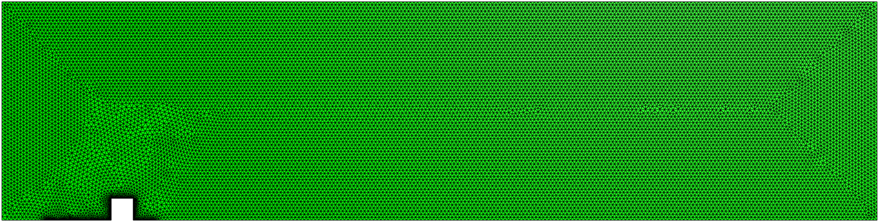
Refer to caption
Figure 17: Example 6. The global triangular mesh plot including the refined grids near the step

We consider computations by 𝐏3bubble\bm{\mathrm{P}}_{3}^{\mathrm{bubble}}-P2dc\mathrm{P}_{2}^{\mathrm{dc}}-𝐁𝐃𝐌3\bm{\mathrm{BDM}}_{3} performed on a locally refined triangular mesh presented in Figure 17. Here we take hl=1/30h_{l}=1/30 and hg=1/6h_{g}=1/6. Note that the Reynolds number is given by Re=1ν\mathrm{Re}=\frac{1}{\nu} here. By adopting the updated Newton iteration (5.3), the problem is first solved for Re=10\mathrm{Re}=10, then Re=25\mathrm{Re}=25, and then in steps of 2525 until Re=1000\mathrm{Re}=1000, with the solution for the previous value of Re\mathrm{Re} used as initial guess for the next; the Stokes equations are solved to provide the initial guess used at Re=10\mathrm{Re}=10.

Refer to caption
Refer to caption
Refer to caption
Refer to caption
Figure 18: Example 6. Streamline on colored velocity magnitude distribution for Re=10\mathrm{Re}=10, 5050, 100100 and 200200 from top-left to bottom-right
Refer to caption
(a) Fragos et al. [15]
Refer to caption
(b) 𝐏3bubble\bm{\mathrm{P}}_{3}^{\mathrm{bubble}}-P2dc\mathrm{P}_{2}^{\mathrm{dc}}-𝐁𝐃𝐌3\bm{\mathrm{BDM}}_{3}
Figure 19: Example 6. A magnified view of streamline contours near the step for Re=275\mathrm{Re}=275. Comparison between Fragos et al. [15] (left) and 𝐏3bubble\bm{\mathrm{P}}_{3}^{\mathrm{bubble}}-P2dc\mathrm{P}_{2}^{\mathrm{dc}}-𝐁𝐃𝐌3\bm{\mathrm{BDM}}_{3} (right)

In Figure 18, it is observed that the streamlines are relatively stable for lower Reynolds numbers (Re⩽200\mathrm{Re}\leqslant 200). On the global perspective, there are a growing but stable eddy in the front of the step and a more apparently growing eddy behind the step; the eddy behind the step expands rapidly towards the outlet as the Reynolds number increases. It is worth mentioning that these results match the experimental results shown in [15] involving the sizes, the shapes and the center location x​yxy-coordinates of the eddies. In particular, when Re⩾275\mathrm{Re}\geqslant 275, in [15] the computational domain is shrunk by about 65% with the same width but a much shorter length 13.5. We still compare the streamline contours near the step by 𝐏3bubble\bm{\mathrm{P}}_{3}^{\mathrm{bubble}}-P2dc\mathrm{P}_{2}^{\mathrm{dc}}-𝐁𝐃𝐌3\bm{\mathrm{BDM}}_{3} for Re=275\mathrm{Re}=275 with that of Fragos et al. [15]. The comparison is presented in Figure 19, and one can find two results are virtually identical, which implies the velocity distribution near the step is independent of the channel length at Re=275\mathrm{Re}=275.

As the Reynolds number further increasing up to 600, a first important difference highlighted by the results shown in Figure 20 that the eddy behind the step starts continuous detachment, which looks like mitosis. In addition, these eddies still move towards the outlet collectively. Another interesting phenomenon is the appearance of an eddy clinging to the bottom at about a quarter of the channel from the r.h.s. at Re=450\mathrm{Re}=450, and this eddy keeps growing and simultaneously moving towards the outlet. It happens that there is a similar case that the formation of another eddy occurs near the above described eddy at Re=500\mathrm{Re}=500. But contrarily, its shape and size change rapidly, and the speed of expanding towards the step is visibly faster than towards the outlet. We also note the difference at the top right corner of the channel that an incomplete eddy forms and keeps moving down slowly. According to the numerical results at various Reynolds numbers provided in [15], we believe that the appearance of this eddy is mainly due to the insufficient length of the channel and the Neumann boundary condition imposed at the outlet.

Refer to caption
Refer to caption
Refer to caption
Refer to caption
Figure 20: Example 6. Streamline on colored velocity magnitude distribution for Re=400\mathrm{Re}=400, 450450, 500500 and 600600 from top-left to bottom-right

All of the above descriptions still hold for higher Reynolds numbers (Re⩾850\mathrm{Re}\geqslant 850), which are supported in Figure 21. In addition, there is an unexpected phenomenon that the eddy, which stems from one debuting at Re=500\mathrm{Re}=500, coalesces continuously with a smaller eddy clinging to the back of the step, and becomes a large eddy independent of that existing behind the step since the beginning. With a magnified view, a detailed plot of streamline contours near the step for these Reynolds numbers is presented in Figure 22 to observe this evolution with a better perspective. Further the contours of velocity magnitude and kinetic pressure at Re=1000\mathrm{Re}=1000 are also plotted in Figure 23. Both of the velocity and the kinetic pressure distributions present dramatic changes near the bottom of the outlet.

Refer to caption
Refer to caption
Refer to caption
Refer to caption
Figure 21: Example 6. Streamline on colored velocity magnitude distribution for Re=850\mathrm{Re}=850, 900900, 950950 and 10001000 from top-left to bottom-right
Refer to caption
Refer to caption
Refer to caption
Refer to caption
Figure 22: Example 6. A magnified view of streamline contours near the step for Re=850\mathrm{Re}=850, 900900, 950950 and 10001000 from left to right
Refer to caption
Refer to caption
Figure 23: Example 6. Contours of velocity magnitude (left) and kinetic pressure (right) for Re=1000\mathrm{Re}=1000

5.7 Example 7: Channel flow past forward-backward facing steps and around square solid objects

At the end of the last example, it is pointed out that both of the velocity and the kinetic pressure distributions change rapidly near the bottom of the outlet at Re=1000\mathrm{Re}=1000. Hence, we are driven to consider how a geometric change of the channel affects the velocity distribution and/or the kinetic pressure distribution. To this end, the same test case as the last example will be implemented but with a modified channel flow region. In this example, the channel dimensions are 40×1040\times 10 with two 1×11\times 1 steps placed five units into the bottom and the top of channel from the l.h.s. respectively, and two 1×11\times 1 solid objects fixed two units over the lower step and two units under the upper step respectively.

Refer to caption
Figure 24: Example 7. The global triangular mesh plot including the refined grids near the steps and the objects
Refer to caption
Refer to caption
Refer to caption
Refer to caption
Figure 25: Example 7. Contours of velocity magnitude for Re=50\mathrm{Re}=50, 100100, 150150 and 300300 from top-left to bottom-right
Refer to caption
Refer to caption
Refer to caption
Refer to caption
Figure 26: Example 7. Contours of kinetic pressure for Re=50\mathrm{Re}=50, 100100, 150150 and 300300 from top-left to bottom-right
Refer to caption
Refer to caption
Refer to caption
Refer to caption
Figure 27: Example 7. Streamline on colored velocity magnitude distribution for Re=50\mathrm{Re}=50, 100100, 150150 and 300300 from top-left to bottom-right
Refer to caption
Refer to caption
Figure 28: Example 7. A magnified view of streamline on colored velocity magnitude distribution near the steps and the objects for Re=150\mathrm{Re}=150 (left) and Re=300\mathrm{Re}=300 (right)

We consider computations still by 𝐏3bubble\bm{\mathrm{P}}_{3}^{\mathrm{bubble}}-P2dc\mathrm{P}_{2}^{\mathrm{dc}}-𝐁𝐃𝐌3\bm{\mathrm{BDM}}_{3} performed on a locally refined triangular mesh presented in Figure 24. Here we take hl=1/40h_{l}=1/40 and hg=1/8h_{g}=1/8 to employ a finer mesh. Note that the Reynolds number is still given by Re=1ν\mathrm{Re}=\frac{1}{\nu} here. By adopting the updated Newton iteration (5.3), the problem is first solved for Re=10\mathrm{Re}=10, then Re=25\mathrm{Re}=25, and then in steps of 2525 until Re=300\mathrm{Re}=300, with the solution for the previous value of Re\mathrm{Re} used as initial guess for the next; the Stokes equations are solved to provide the initial guess used at Re=10\mathrm{Re}=10.

The contours of velocity magnitude, and the contours of kinematic pressure, and the streamlines at various Reynolds numbers Re=50\mathrm{Re}=50, 100100, 150150 and 300300 are presented in Figures 25, 26 and 27 respectively. Indeed, the added step and two small square solid objects change the distributions dramatically. Specifically, the complete symmetries occur over the whole channel; in the region near the outlet, the velocity magnitude shows the two-level differentiation while the kinematic pressure keeps constant. For the streamlines, the most remarkable feature is that two large eddies behind the steps, whose scale is larger at the same Reynolds number by comparison with that of the last example, compress the “jet flow” region in the middle of the channel. Another interesting phenomenon is that the distribution change of the streamlines slows down as the Reynolds number increases. To verify this statement over all the channel, a detailed plot of streamline contours near the steps and the objects for Re=150\mathrm{Re}=150 and 300300 is presented in Figure 28 with a magnified view.

6 Conclusion

Based on the classical mixed method with high-order conforming finite elements, we have developed an efficient pressure-robust method to the rotation form of the stationary incompressible Navier–Stokes equations over shape-regular triangular meshes via constructing a novel skew-symmetric discrete trilinear form containing the velocity reconstruction operator. The proposed method achieves the pressure-independent velocity errors and preserves the same convergence orders of both velocity and pressure as the classical method does. Three numerical examples with exactly analytical solutions have presented to verify the theoretical results and to show the remarkable performance in the aspect of errors compared to the classical method. Furthermore, four practical experiments are implemented to adequately demonstrate the efficiency and robustness of the proposed high-order finite element method.

References

References

  • [1] N. Ahmed, A. Linke, C. Merdon, Towards Pressure-Robust Mixed Methods for the Incompressible Navier–Stokes Equations, Comput. Methods Appl. Math. 18 (3) (2018) 353–372. doi:10.1515/cmam-2017-0047.
  • [2] I. Babŭska, The finite element method with Lagrangian multipliers, Numer. Math. 20 (1973) 179–192. doi:10.1007/BF01436561.
  • [3] E. Barragy, G. F. Carey, Stream function-vorticity driven cavity solutions using pp finite elements, Comput. fluids 26 (1997) 453–468. doi:10.1016/S0045-7930(97)00004-2.
  • [4] D. Boffi, F. Brezzi, M. Fortin, Mixed Finite Element Methods and Applications, Springer-Verlag, Berlin, Heidelberg, 2013. doi:10.1007/978-3-642-36519-5.
  • [5] O. Botella, R. Peyret, Benchmark spectral results on the lid-driven cavity flow, Comput. fluids 27 (4) (1998) 421–433. doi:10.1016/S0045-7930(98)00002-4.
  • [6] F. Brezzi, On the existence, uniqueness and approximation of saddle-point problems arising from Lagrangian multipliers, RAIRO Anal. Numer. R2 (1974) 129–151. doi:10.1051/m2an/197408R201291.
  • [7] J. M. Cadou, M. Potier-Ferry, B. Cochelin, N. Damil, ANM for stationary Navier–Stokes equations and with Petrov-Galerkin formulation, Int. J. Numer. Meth. Eng. 50 (2001) 825–845. doi:10.1002/1097-0207(20010210)50:4<825::AID-NME53>3.0.CO;2-0.
  • [8] D. Cioranescu, V. Girault, K. R. Rajagopal, Mechanics and Mathematics of Fluids of the Differential Type, Advances in Mechanics and Mathematics 35, Springer, Cham, Switzerland, 2016. doi:10.1007/978-3-319-39330-8.
  • [9] B. Cockburn, G. Kanschat, D. Schötzau, C. Schwab, Local Discontinuous Galerkin Methods for the Stokes System, SIAM J. Numer. Anal. 40 (1) (2002) 319–343. doi:10.1137/S0036142900380121.
  • [10] D. A. Di Pietro, J. Droniou, A hybrid high-order method for Leray–Lions elliptic equations on general meshes, Math. Comput. 86 (307) (2017) 2159–2191. doi:10.1090/mcom/3180.
  • [11] E. Erturk, T. C. Corke, C. Gökçöl, Numerical solutions of 2-D steady incompressible driven cavity flow at high Reynolds numbers, Int. J. Numer. Meth. Fluids 48 (2005) 747–774. doi:10.1002/fld.953.
  • [12] P. E. Farrell, L. Mitchell, L. R. Scott, F. Wechsung, A Reynolds-robust preconditioner for the Scott-Vogelius discretization of the stationary incompressible Navier–Stokes equations, SMAI Journal of Computational Mathematics 7 (2021) 75–96. doi:10.5802/smai-jcm.72.
  • [13] P. E. Farrell, L. Mitchell, F. Wechsung, An Augmented Lagrangian Preconditioner for the 3D Stationary Incompressible Navier–Stokes Equations at High Reynolds Number, SIAM J. Sci. Comput. 41 (5) (2019) A3073–A3096. doi:10.1137/18M1219370.
  • [14] J. A. Fiordilino, W. Layton, Y. Rong, An efficient and modular grad-div stabilization, Comput. Methods Appl. Mech. Engrg. 335 (2018) 327–346. doi:10.1016/j.cma.2018.02.023.
  • [15] V. P. Fragos, S. P. Psychoudaki, N. A. Malamataris, Computer-aided analysis of flow past a surface-mounted obstacle, Int. J. Numer. Meth. Fluids 25 (5) (1997) 495–512. doi:10.1002/(sici)1097-0363(19970915)25:5<495::aid-fld571>3.0.co;2-d.
  • [16] L. P. Franca, A. Nesliturk, On a two-level finite element method for the incompressible Navier–Stokes equations, Int. J. Numer. Meth. Eng. 52 (2001) 433–453. doi:10.1002/nme.220.
  • [17] K. Galvin, A. Linke, L. Rebholz, N. Wilson, Stabilizing poor mass conservation in incompressible flow problems with large irrotational forcing and application to thermal convection, Comput. Methods Appl. Mech. Engrg. 237 (2012) 166–176. doi:10.1016/j.cma.2012.05.008.
  • [18] N. R. Gauger, A. Linke, P. W. Schroeder, On high-order pressure-robust space discretisations, their advantages for incompressible high Reynolds number generalised Beltrami flows and beyond, SMAI Journal of Computational Mathematics, 5 (2019) 89–129. doi:10.5802/smai-jcm.44.
  • [19] U. Ghia, K. N. Ghia, C. T. Shin, High-Re solutions for incompressible flow using the Navier–Stokes equations and a multigrid method, J. Comput. Phys. 48 (3) (1982) 387–411. doi:10.1016/0021-9991(82)90058-4.
  • [20] V. Girault, P. A. Raviart, Finite Element Methods for Navier–Stokes Equations, Springer-Verlag, Berlin, Heidelberg, 1986. doi:10.1007/978-3-642-61623-5.
  • [21] V. Gravemeier, W. A. Wall, E. Ramm, A three-level finite element method for the instationary incompressible Navier–Stokes equations, Comput. Methods Appl. Mech. Engrg. 193 (15–16) (2004) 1323–1366. doi:10.1016/j.cma.2003.12.027.
  • [22] E. Hachem, B. Rivaux, T. Kloczko, H. Digonnet, T. Coupez, Stabilized finite element method for incompressible flows with high Reynolds number, J. Comput. Phys. 229 (2010) 8643–8665. doi:10.1016/j.jcp.2010.07.030.
  • [23] Y. He, J. Li, Convergence of three iterative methods based on the finite element discretization for the stationary Navier–Stokes equations, Comput. Methods Appl. Mech. Engrg. 198 (2009) 1351–1359. doi:10.1016/j.cma.2008.12.001.
  • [24] Y. He, A. Wang, A simplified two-level method for the steady Navier–Stokes equations, Comput. Methods Appl. Mech. Engrg. 197 (2008) 1568–1576. doi:10.1016/j.cma.2007.11.032.
  • [25] T. J. R. Hughes, G. Engel, L. Mazzei, M. G. Larson, A Comparison of Discontinuous and Continuous Galerkin Methods Based on Error Estimates, Conservation, Robustness and Efficiency. In: B. Cockburn, G. E. Karniadakis, C. W. Shu (eds) Discontinuous Galerkin Methods. Lecture Notes in Computational Science and Engineering, vol 11. Springer, Berlin, Heidelberg, 2000, 135–146. doi:10.1007/978-3-642-59721-3_9.
  • [26] V. John, Finite Element Methods for Incompressible Flow Problems, Springer Series in Computational Mathematics 51, Springer, Cham, Switzerland, 2016. doi:10.1007/978-3-319-45750-5.
  • [27] V. John, Reference values for drag and lift of a two-dimensional time-dependent flow around a cylinder, Int. J. Numer. Meth. Fluids 44 (2004) 777–788. doi:10.1002/fld.679.
  • [28] V. John, A. Liakos, Time-dependent flow across a step: the slip with friction boundary condition, Int. J. Numer. Meth. Fluids 50 (2006) 713–731. doi:10.1002/fld.1074.
  • [29] V. John, A. Linke, C. Merdon, M. Neilan, L. G. Rebholz, On the Divergence Constraint in Mixed Finite Element Methods for Incompressible Flows, SIAM Review 59 (3) (2017) 492–544. doi:10.1137/15M1047696.
  • [30] L. I. G. Kovasznay, Laminar flow behind a two-dimensional grid, Proc. Camb. Philos. Soc. 44 (1) (1948) 58–62. doi:10.1017/s0305004100023999.
  • [31] W. Layton, H. K. Lee, J. Peterson, A defect-correction method for the incompressible Navier–Stokes equations, Appl. Math. Comput. 129 (1) (2002) 1–19. doi:10.1016/S0096-3003(01)00026-1.
  • [32] W. Layton, C. C. Manica, M. Neda, M. Olshanskii, L. G. Rebholz, On the accuracy of the rotation form in simulations of the Navier–Stokes equations, J. Comput. Phys. 228 (9) (2009) 3433–3447. doi:10.1016/j.jcp.2009.01.027.
  • [33] W. Layton, C. C. Manica, M. Neda, L. G. Rebholz, Numerical analysis and computational comparisons of the NS-alpha and NS-omega regularizations, Comput. Methods Appl. Mech. Engrg. 199 (13–16) (2010) 916–931. doi:10.1016/j.cma.2009.01.011.
  • [34] A. Linke, A divergence-free velocity reconstruction for incompressible flows, C. R. Acad. Sci. Paris 350 (17–18) (2012) 837–840. doi:10.1016/j.crma.2012.10.010.
  • [35] A. Linke, On the role of the Helmholtz decomposition in mixed methods for incompressible flows and a new variational crime, Comput. Methods Appl. Mech. Engrg. 268 (2014) 782–800. doi:10.1016/j.cma.2013.10.011.
  • [36] A. Linke, G. Matthies, L. Tobiska, Robust arbitrary order mixed finite element methods for the incompressible Stokes equations with pressure independent velocity errors, ESAIM: M2AN 50 (2016) 289–309. doi:10.1051/m2an/2015044.
  • [37] A. Linke, C. Merdon, On velocity errors due to irrotational forces in the Navier–Stokes momentum balance, J. Comput. Phys. 313 (2016) 654–661. doi:10.1016/j.jcp.2016.02.070.
  • [38] A. Linke, C. Merdon, Pressure-robustness and discrete Helmholtz projectors in mixed finite element methods for the incompressible Navier–Stokes equations, Comput. Methods Appl. Mech. Engrg. 311 (2016) 304–326. doi:10.1016/j.cma.2016.08.018.
  • [39] A. Linke, L. G. Rebholz, On a reduced sparsity stabilization of grad-div type for incompressible flow problems, Comput. Methods Appl. Mech. Engrg. 261–262 (2013) 142–153. doi:10.1016/j.cma.2013.04.005.
  • [40] X. Liu, R. Li, Y. Nie, A divergence-free reconstruction of the nonconforming virtual element method for the Stokes problem, Comput. Methods Appl. Mech. Engrg. 372 (2020) 113351. doi:10.1016/j.cma.2020.113351.
  • [41] X. Liu, Y. Nie, A modified nonconforming virtual element with BDM-like reconstruction for the Navier–Stokes equations, Appl. Numer. Math. 167 (2021) 375–388. doi:10.1016/j.apnum.2021.05.014.
  • [42] C. C. Manica, M. Neda, M. Olshanskii, L. G. Rebholz, N. E. Wilson, On an efficient finite element method for Navier–Stokes–ω¯\overline{\omega} with strong mass conservation, Comput. Methods Appl. Math. 11 (1) (2011) 3–22. doi:10.2478/cmam-2011-0001.
  • [43] L. Mu, A uniformly robust H(div) weak Galerkin finite element methods for Brinkman problems, SIAM J. Numer. Anal. 58 (3) (2020) 1422–1439. doi:10.1137/19M1283604.
  • [44] L. Mu, Pressure robust weak Galerkin finite element methods for Stokes problems, SIAM J. Sci. Comput. 42 (3) (2020) B608–B629. doi:10.1137/19M1266320.
  • [45] L. Mu, X. Ye, S. Zhang, A stabilizer-free, pressure-robust, and superconvergence weak galerkin finite element method for the stokes equations on polytopal mesh, SIAM J. Sci. Comput. 43 (4) (2021) A2614–A2637. doi:10.1137/20M1380405.
  • [46] M. Olshanskii, A low order Galerkin finite element method for the Navier–Stokes equations of steady incompressible flow: a stabilization issue and iterative methods, Comput. Methods Appl. Mech. Engrg. 191 (47–48) (2002) 5515–5536. doi:10.1016/S0045-7825(02)00513-3.
  • [47] M. Olshanskii, A. Reusken, Grad-div stabilization for Stokes equations, Math. Comp. 73 (248) (2004) 1699–1718. doi:10.1090/S0025-5718-03-01629-6.
  • [48] D. C. Quiroz, D. A. Di Pietro, A Hybrid High-Order method for the incompressible Navier–Stokes problem robust for large irrotational body forces, Comput. Math. Appl. 79 (2020) 2655–2677. doi:10.1016/j.camwa.2019.12.005.
  • [49] Y. Rong, J. A. Fiordilino, Numerical Analysis of a BDF2 Modular Grad-Div Stabilization Method for the Navier–Stokes Equations, J. Sci. Comput. 82 (2020) 66. doi:10.1007/s10915-020-01165-5.
  • [50] M. Schäfer, S. Turek, F. Durst, E. Krause, R. Rannacher, Benchmark Computations of Laminar Flow Around a Cylinder, Flow Simul. High-Perform. Comput. II 48 (1996) 547–566. doi:10.1007/978-3-322-89849-4_39.
  • [51] J. Schöberl, C++11 Implementation of Finite Elements in NGSolve, ASC Report 30/2014, Institute for Analysis and Scientific Computing, Vienna University of Technology, 2014.
  • [52] R. Temam, Navier–Stokes Equations: Theory and Numerical Analysis, 3rd Edition, AMS, Providence, Rhode Island, 1984. doi:10.1090/chel/343.
  • [53] M. Van Dyke, An Album of Fluid Motion, 12th Edition, The Parabolic Press, Stanford, California, 2008.
  • [54] M. Van Dyke, Perturbation Methods in Fluid Mechanics, Annotated Edition, The Parabolic Press, Stanford, California, 1975.
  • [55] G. Wang, L. Mu, Y. Wang, Y. He, A pressure-robust virtual element method for the Stokes problem, Comput. Methods Appl. Mech. Engrg. 382 (2021) 113879. doi:10.1016/j.cma.2021.113879.