Self-Adaptive Deep Neural Network:
Numerical Approximation to Functions and PDEs Thanks: This work was supported in part by the National Science Foundation under grant DMS-2110571.

Deep neural network (DNN) has achieved astonishing performance in computer vision, natural language processing, and many other artificial intelligence (AI) tasks (see, e.g., [8, 16, 12]). This success encourages wide applications to other fields, including recent studies of using DNN models to learn solutions of partial differential equations (PDEs) (see, e.g., [2, 7, 5, 10, 20, 23]). The phenomenal performance on many AI tasks comes at the cost of high computational complexity. Accordingly, designing efficient network architectures for DNN is an important step towards enabling the wide deployment of DNN in various applications.

Studies and applications of neural network (NN) may be traced back to the work of Hebb [14] in the late 1940’s and Rosenblatt [21] in the 1950’s. DNN produces a new class of functions through compositions of linear transformations and activation functions. This class of functions is extremely rich. For example, it contains piece-wise polynomials, which are the footing of spectral elements, and continuous and discontinuous finite element methods for computer simulations of complex physical, biological, and human-engineered systems. It approximates polynomials of any degree with exponential efficiency, even using simple activation functions like ReLU. More importantly, a neural network function can automatically adapt to a target function or the solution of a PDE.

Despite great successes of DNN in many practical applications, it is widely accepted that approximation properties of DNN are not yet well understood and that understanding on why and how they work could lead to significant improvements in many machine learning applications. First, some empirical observations suggest that deep network can approximate many functions more accurately than shallow network, but rigorous study on the theoretical advantage of deep network is scarce. Therefore, even in the manual design of network models, the addition of neurons along depth or width is ad-hoc. Second, current methods on design of the architecture of DNN in terms of their width and depth are empirical. Tuning of depth and width is tedious, mainly from experimental results in ablation studies which typically require domain knowledge about the underlying problem. Third, there is a tendency in practice to use over-parametrized neural networks; this leads to a high-dimensional nonlinear optimization problem which is much more difficult to train than a low-dimensional one. These considerations suggest that a fundamental, open question to be addressed in scientific machine learning is: what is the optimal network model required, in terms of width, depth, and the number of parameters, to learn data, a function, or the solution of a PDE within some prescribed accuracy?

To address this issue, we introduce a self-adaptive algorithm: the adaptive network enhancement (ANE) method, written as loops of the form

$\mbox{\bf train }\rightarrow\,\,\,\mbox{\bf estimate }\rightarrow\,\,\,\mbox{\bf enhance}.$

To develop an efficient ANE method, we need to address the following essential questions at each adaptive step when the current NN is not sufficient for the given task:

• (a)

  how many new neurons should be added?

• (b)

  when should a new layer be added?

For a two-layer NN, we proposed the ANE method (see Algorithm 4.1) for learning a given function in [18] and the solution of a given self-adjoint elliptic PDEs through the Ritz formulation in [17]. In the case of a two-layer NN, question (b) is irrelevant and question (a) was addressed by introducing a network enhancement strategy that decides the number of new neurons to be added in the first hidden layer. This strategy is based on the physical partition of the current computer simulation determined by the a posteriori error indicators (see Algorithm 3.1).

For a multi-layer NN, it is challenging to address both the questions. First, the role of a neuron in approximation at a hidden layer varies and depends on which hidden layer the neuron is located. Second, there is almost no understanding on the role of a specific hidden layer in approximation and, hence, we have no a priori approximation information for determining when a new layer should be added. To resolve question (a) for a multi-layer, we will exploit the geometric property of the current computer simulation and introduce a novel enhancement strategy (see Algorithm 4.2) that determines the number of new neurons to be added at a hidden layer other than the first hidden layer. For question (b), we will introduce a computable quantity to measure the improvement rate of two consecutive NNs per the relative increase of parameters. When the improvement rate is small, then a new layer is started.

Training DNN, i.e., determining the values of the parameters of DNN, is a problem in nonlinear optimization. This high dimensional, nonlinear optimization problem tends to be computationally intensive and complicated and is usually solved iteratively by the method of gradient descent and its variations (see [4]). In general, a nonlinear optimization has many solutions, and the desired one is obtained only if we start from a close enough first approximation. A common way to obtain a good initialization is by the method of continuation [1]. The ANE method provides a natural process for obtaining a good initialization. Basically, the approximation at the previous NN is already a good approximation to the current NN in the loops of the ANE method. To provide a better approximation, we initialize the weights and bias of newly added neurons at the first hidden layer by using the physical partition of the domain (see Section 3 and [18] for details); in this paper we introduce an advanced procedure on how to initialize newly added neurons at a hidden layer that is not the first hidden layer.

For simplicity of presentation, the ANE method for a multi-layer NN is first described for learning a given function through the least-squares loss function (see Section 4). The method is then applied to learn solutions of linear advection-reaction equations through the least-squares neural network (LSNN) method introduced in [6] (see Section 7). We demonstrate that the ANE method can automatically design a nearly minimal NN for learning functions exhibiting sharp transitional layers as well as discontinuous solutions of hyperbolic PDEs.

Recently, there is growing interest in automatic machine learning (AutoML) in an effort of replacing a manual design process of architectures by human experts. Neural architecture search (NAS) method (see a survey paper [11] and reference therein) presents a general methodology at high level on AutoML. It consists of three components: search space, search strategy, and performance estimation strategy. Usually the resulting algorithm is computationally intensive because it explores a wide range of potential network architectures. Nevertheless, the NAS outperforms manually designed architectures in accuracy on some tasks such as image classification, object detection, or semantic segmentation. The NAS based on the physics-informed neural network is recently used for solving stochastic groundwater flow problem in [13].

The paper is organized as follows. DNN, the best least-squares (LS) approximation to a given function using DNN, and the discrete counterpart of the best LS approximation are introduced in Section 2. The physical partition for a DNN function is described in Section 3. The ANE method, initialization of parameters at different stage, and numerical experiments are presented in Sections 4, 5, and 6, respectively. Finally, application of the ANE method to the linear advection-reaction equation is given in Section 7.

A deep neural network defines a function of the form

where $d$ is the dimension of input ${\bf x}$, $\mbox{\boldmath${\omega}$}^{(L)}\in\mathbb{R}^{n_{L-1}}$, $b^{(L)}\in\mathbb{R}$, the symbol $\circ$ denotes the composition of functions, and $L$ is the depth of the network. For $l=1,\cdots,L-1$, the $N^{(l)}\!:\mathbb{R}^{n_{l-1}}\!\rightarrow\mathbb{R}^{n_{l}}$ is called the $l^{th}$ hidden layer of the network defined by

where $\mbox{\boldmath${\omega}$}^{(l)}\in\mathbb{R}^{n_{l}\times n_{l-1}}$, ${\bf b}^{(l)}\in\mathbb{R}^{n_{l}}$, ${\bf x}^{(0)}={\bf x}$, and $\sigma(t)=\max\{0,t\}^{p}$ with positive integer $p$ is the activation function and its application to a vector is defined component-wise. This activation function is referred to as a spline activation ReLU^p. When $p=1$, $\sigma(t)$ is the popular rectified linear unit (ReLU). There are many other activation functions such as (logistic, Gaussian, arctan) sigmoids (see, e.g., [19]).

Let ${\theta}$ denote all parameters to be trained, i.e., the weights $\{\mbox{\boldmath${\omega}$}^{(l)}\}_{l=1}^{L}$ and the bias $\{{\bf b}^{(l)}\}_{l=1}^{L}$. Then the total number of parameters is given by

Denote the set of all DNN functions by

Let $f({\bf x})\in\mathbb{R}$ be a given target function defined in a domain $\Omega\in\mathbb{R}^{d}$. Training DNN to learn the function $f({\bf x})$ using least-squares loss function amounts to solve the following best least-squares approximation: find $f_{N}({\bf x};{\small\mbox{\boldmath${\theta}$}}^{*})\in{\cal M}_{N}({\small\mbox{\boldmath${\theta}$}},L)$ such that

where $v({\bf x};{\small\mbox{\boldmath${\theta}$}})\in{\cal M}_{N}({\small\mbox{\boldmath${\theta}$}},L)$ is of the form

with $N^{(l)}(\cdot)$ defined in (2), and $\|v(\cdot)\|=\left(\int_{\Omega}v^{2}({\bf x})\,d{\bf x}\right)^{1/2}$ is the $L^{2}(\Omega)$ norm.

Let ${\cal I}$ be the integral operator over the domain $\Omega$ given by

Let ${\cal T}=\{K\,:\,K\mbox{ is an open subdomain of }\Omega\}$ be a partition of the domain $\Omega$, i.e., union of all subdomains of ${\cal T}$ equals to the whole domain $\Omega$ and that any two distinct subdomains of ${\cal T}$ have no intersection. Let ${\cal Q}_{{}_{\cal T}}$ be a quadrature operator based on the partition ${\cal T}$, i.e., ${\cal I}(v)\approx{\cal Q}_{{}_{\cal T}}\big(v\big)$, such that

defines a weighted $l_{2}$-norm. The best discrete least-squares approximation with numerical integration over the partition ${\cal T}$ is to find $f_{{}_{\cal T}}({\bf x};{{\small\mbox{\boldmath${\theta}$}}^{*}_{{}_{\cal T}}})\in{\cal M}_{N}({\small\mbox{\boldmath${\theta}$}},L)$ such that

As seen in [18], the physical partition of the current NN approximation plays a critical role in the ANE method for a two-layer NN. As we shall see, it is essential for our self-adaptive multi-layer NN as well. For simplicity of presentation, we consider ReLU activation function only in this section. The idea of our procedure for determining the physical partition can be easily extended to other activation functions even though the corresponding geometry becomes complex.

For any function $v\in{\cal M}_{N}(\mbox{\boldmath${\theta}$},k)$ with $k\geq 2$, it is easy to see that $v$ is a continuous piece-wise linear function with respect to a partition $\mathcal{K}^{(k-1)}$ of the domain $\Omega$. This partition is referred to as the physical partition of the function $v$ in ${\cal M}_{N}(\mbox{\boldmath${\theta}$},k)$. This section describes how to determine the physical partition $\mathcal{K}^{(k-1)}$ of a function in ${\cal M}_{N}(\mbox{\boldmath${\theta}$},k)$. To this end, for $l=1,\,\cdots,\,k-1$, denote by ${\cal K}^{(l)}$ the physical partition of the first $l$ layers.

To determine the physical partition ${\cal K}^{(1)}$, notice that a two-layer NN with $n_{1}$ neurons generates the following set of functions:

where ${\cal S}^{d-1}$ is the unit sphere in $\mathbb{R}^{d}$. The ${\cal M}_{N}({\small\mbox{\boldmath${\theta}$}},2)$ may be viewed as an extension of the free-knot spline functions [22] to multi-dimension, and its free breaking hyper-planes are

This suggests that the physical partition ${\cal K}^{(1)}$ is formed by the boundary of the domain $\Omega$ and the hyper-planes $\left\{\mbox{\boldmath${\omega}$}^{(1)}_{j}\cdot{\bf x}-b^{(1)}_{j}=0\right\}_{j=1}^{n_{1}}$.

Next, we describe how to form the physical partition ${\cal K}^{(l)}$. Our procedure is based on the observation that for $l=2,\,...\,,k-1$, the ${\cal K}^{(l)}$ may be viewed as a refinement of the ${\cal K}^{(l-1)}$. For $j=1,\,\cdots,\,n_{l}$, denote the function generated by the $j^{\text{th}}$ neuron at the $l^{\text{th}}$-layer without the activation function by

where ${\bf x}^{(l-2)}=N^{(l-2)}\circ\cdots\circ N^{(1)}({\bf x})$. It is clear that the functions $g_{j}^{(l)}({\bf x})$ are continuous piece-wise linear functions with respect to the physical partition ${\cal K}^{(l-1)}$. The action of the activation function on $g_{j}^{(l)}({\bf x})$, i.e., $\sigma(g_{j}^{(l)}({\bf x}))=\max\{0,g_{j}^{(l)}({\bf x})\}$ for $j=1,\,\cdots,\,n_{l}$, generate $n_{l}$ continuous piece-wise linear functions with respect to a refined partition of ${\cal K}^{(l-1)}$. Therefore, the refinement is created by the activation function through replacing negative values of $g_{j}^{(l)}({\bf x})$ by zero (see Fig. 1 for illustration). In other words, the refinement is done by all new hyper-planes satisfying

To determine whether or not an element $K\in{\cal K}^{(l-1)}$ is refined, for each $g_{j}^{(l)}({\bf x})$, we compute its values at vertices of $K$. If these values change signs, then the element $K$ is partitioned by the hyper-plane $g_{j}^{(l)}({\bf x})=0$ into two subdomains. It is possible that an element $K\in{\cal K}^{(l-1)}$ may be partitioned by many hyper-planes in (10). Denote the collection of refined elements in ${\cal K}^{(l-1)}$ by

Denote by ${\cal K}^{(l)}_{K}$ the physical partition of element $K\in{\cal K}^{(l-1)}$ by hyper-planes in (10) and the boundary of $K$. Then the physical partition ${\cal K}^{(l)}$ by the first $l$ hidden layers is given by

The procedure of determining the physical partition of a function in ${\cal M}_{N}({\small\mbox{\boldmath${\theta}$}},k)$ with $k\geq 3$ is summarized in Algorithm 3.1.

Given a target function $f({\bf x})$ and a prescribed tolerance $\epsilon>0$ for approximation accuracy, in [18] we proposed the adaptive network enhancement (ANE) method for generating a two-layer ReLU NN and a numerical integration mesh such that

where $f_{{}_{\cal T}}({\bf x};{{\small\mbox{\boldmath${\theta}$}}^{*}_{{}_{\cal T}}})$ is the solution of the optimization problem in (6) over a two-layer NN with numerical integration defined on the partition ${\cal T}$.

For the convenience of readers and needed notations, we state Algorithm 5.1 of [18] (see Algorithm 4.1 below) for the case that numerical integration based on a partition ${\cal T}$ is sufficiently accurate. In this algorithm, ${\cal K}$ is the physical partition of the current approximation $f_{{}_{\cal T}}$, $\xi_{{}_{K}}=\|f-f_{{}_{\cal T}}\|_{{}_{K,{\cal T}}}$ is the local error in the physical subdomain $K\in{\cal K}$, and the network enhancement strategy introduced in [18] consists of either the average marking strategy:

where $\#{\cal K}$ is the number of elements of ${\cal K}$, or the bulk marking strategy: finding a minimal subset $\hat{{\cal K}}$ of ${\cal K}$ such that

With the subset $\hat{{\cal K}}$, the number of new neurons to be added to the current NN is equal to $\#\hat{{\cal K}}$, the number of elements in $\hat{{\cal K}}$.

For continuous functions exhibiting intersecting interface singularities or sharp transitional layer like discontinuities, numerical results in [18] showed the efficacy of the ANE method for generating a nearly minimal two-layer NN to learn the target function within the prescribed accuracy. However, in the case that the transitional layer is over a circle but not a straight line, the approximation by a two-layer NN with a large number of neurons exhibits a certain level of oscillation; while the approximation using a three-layer NN with a small number of parameters is more accurate than the former and has no oscillation. Those numerical experiments suggest that a three-layer NN is needed for learning certain type of functions even if they are continuous.

In this section, we develop the ANE method for a multi-layer NN. To address question (b), i.e., when to add a new layer, we introduce a computable quantity denoted by $\eta_{r}$ measuring the improvement rate of two consecutive NNs per the relative increase of parameters. If the improvement rate $\eta_{r}$ is less than or equal to a prescribed expectation rate $\delta\in(0,2)$, i.e.,

for two consecutive ANE runs, then the ANE method adds a new layer. Otherwise, the ANE adds neurons to the last hidden layer of the current network. Here a conservative strategy for adding a new layer is adopted by a double-run to check if inefficiency is identified when enhancing neurons in the current layer.

To define the improvement rate, denote the two consecutive NNs by ${\cal M}_{\scriptscriptstyle N^{\text{new}}}$ and ${\cal M}_{\scriptscriptstyle N^{\text{old}}}$, where the subscripts $N^{\text{new}}$ and $N^{\text{old}}$ are the number of parameters of these two NNs, respectively. Assume that the former is obtained by adding neurons in the last hidden layer of the latter. Let $\xi^{\text{new}}$ and $\xi^{\text{old}}$ be the error estimators of the approximations using ${\cal M}_{\scriptscriptstyle N^{\text{new}}}$ and ${\cal M}_{\scriptscriptstyle N^{\text{old}}}$, respectively. The improvement rate $\eta_{r}$ is defined as

where $r$ is the order of the approximation with respect to the number of parameters and may depend on the activation function and the layer.

To determine the number of new neurons to be added in the last (but not first) hidden layer, our network enhancement strategy starts with the marked subset $\hat{{\cal K}}$ of ${\cal K}$ as in the first layer, where ${\cal K}$ is the physical partition of the current approximation. The subset $\hat{{\cal K}}$ is further regrouped into a new set $\mathcal{C}=\{C:\,C\mbox{ is a connected, open subdomain of }\Omega\}$ such that each element of $\mathcal{C}$ is either an isolated subdomain in $\hat{{\cal K}}$ or a union of connected subdomains in $\hat{{\cal K}}$. Now, the number of new neurons to be added equals to the number of elements in $\mathcal{C}$. This strategy is based on the observation that a multi-layer NN is capable of generating piece-wise breaking hyper-planes in connected subdomains by one neuron. Summarizing the above discussion, our network enhancement strategy on adding neurons and layers is described in Algorithm 4.2.

Assume that numerical integration on ${\cal T}$ is accurate, then the ANE method for generating a nearly minimal multi-layer neural network is described in Algorithm 4.3.

To determine the values of the network parameters, we need to solve the optimization problem in (6), which is non-convex and, hence, computationally intensive and complicated. Currently, this problem is often solved by iterative optimization methods such as gradient descent (GD), Stochastic GD, Adam, etc. (see, e.g., [4] for a review paper in 2018 and references therein). Since non-convex optimizations usually have many solutions and/or many local minimum, it is then critical to start with a good initial guess in order to obtain the desired solution. As seen in [18], the ANE method itself is a natural continuation process for generating good initializations. In this section, we discuss initialization strategies of the ANE method for a multi-layer NN in two dimensions. Extensions to three dimensions are straightforward conceptually but more complicated algorithmically.

There are three cases that need to be initialized: (1) the beginning of the ANE method for a two-layer NN with a small number of neurons; (2) adding new neurons at the first layer; and (3) adding new neurons at the last hidden layer which is not the first layer. Initialization for both cases (1) and (2) was introduced in Section 5 of [18]. For the convenience of readers, we briefly describe them below.

The ANE method starts with a two-layer NN with $n_{1}$ neurons. Denote the input weights and bias by $\mbox{\boldmath${\omega}$}^{(1)}=\left(\mbox{\boldmath${\omega}$}^{(1)}_{1},...,\mbox{\boldmath${\omega}$}^{(1)}_{n_{1}}\right)^{T}$ and ${\bf b}^{(1)}=\left(b^{(1)}_{1},...,b^{(1)}_{n_{1}}\right)^{T}$, respectively; and the output bias and weights by ${\bf c}^{(1)}=\left(b^{(2)},\omega_{1}^{(2)},...,\omega_{n_{1}}^{(2)}\right)^{T}$. The initials of $\mbox{\boldmath${\omega}$}^{(1)}$ and ${\bf b}^{(1)}$ are chosen such that the hyper-planes

partition the domain uniformly. With the initial $\mbox{\boldmath${\theta}$}^{(1)}=(\mbox{\boldmath${\omega}$}^{(1)},{\bf b}^{(1)})$ prescribed above, let

Then the initial of ${\bf c}^{(1)}$ is given by the solution of the following system of linear algebraic equations

where the coefficient matrix $\bm{M}(\mbox{\boldmath${\theta}$}^{(1)})$ and the right-hand side vector $F(\mbox{\boldmath${\theta}$}^{(1)})$ are given by

respectively.

When adding new neurons at the first layer, the parameters associated with the old neurons will inherit the current approximation as their initials and those of the new neurons are initialized through the corresponding hyper-planes. Each new neuron is related to a sub-domain $K\in\hat{{\cal K}}$ (see Algorithm 4.1) and is initialized by setting its corresponding hyper-plane to pass through the centroid of $K$ and orthogonal to the direction vector with the smallest variance of quadrature points in $K$. For details, see Section 5 of [18].

In the case (3), new neurons are added either at a new layer or at the current but not the first layer. As in the case (2), the parameters of the old neurons are initialized with their current approximations. Below we describe our strategy on how to initialize newly added neurons. First, consider the case in which we add neurons to start a new layer. Assume that the current NN has $k-1$ hidden layers. By Algorithm 4.2, the number of new neurons to be added at the $k^{\text{th}}$ hidden layer equals to the number of elements in $\mathcal{C}^{(k-1)}$. For each element $C\in\mathcal{C}^{(k-1)}$, one neuron is added to the $k^{\text{th}}$ hidden layer, and its output weight is randomly initialized. Below we introduce a strategy to initialize its bias and weights, $\mbox{\boldmath${\omega}$}^{(k)}=\left(b^{(k)},\,\omega_{1}^{{(k)}},\cdots,\omega^{{(k)}}_{n_{k-1}}\right)^{T}=\left(\omega_{0}^{{(k)}},\,\omega_{1}^{{(k)}},\cdots,\omega^{{(k)}}_{n_{k-1}}\right)^{T}$. To this end, let us introduce a corresponding output function of the neuron to be added to refine $C$,

where the functions $\{\varphi^{(k-1)}_{i}({\bf x})\}_{i=0}^{n_{k-1}}$ are given by

Note that $C\in\mathcal{C}^{(k-1)}$ is either an isolated physical subdomain or consists of several connected physical sub-domains in $\hat{{\cal K}}^{(k-1)}$.

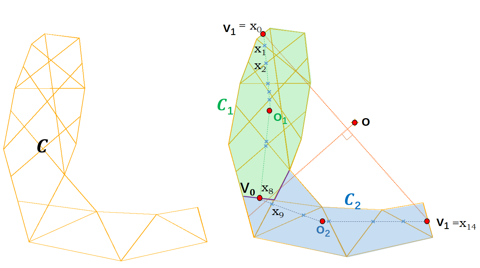
A heuristic method is introduced here to initialize a neuron such that its corresponding break poly-lines can divide the sub-domains in $C$ as many as possible (please refer to Fig. 2 for a graphical illustration):

• •

  step 0: Initialize an empty set $X=\emptyset$;

• •

  step 1: Compute pairwise distances among mid-points on the boundary edges of $C$, find the point pair $({\bf v}_{1},{\bf v}_{2})$ having the longest distance;

• •

  step 2: Compute the centroid ${\bf o}$ of $C$;

• •

  step 3: If ${\bf o}\in C$, find the set of intersection points of the edges in $C$ and the two line segments $\overline{{\bf o}{\bf v}_{1}}$ and $\overline{{\bf o}{\bf v}_{2}}$. Add the set of intersection points into $X$;

• •

  step 4: If ${\bf o}\notin C$, decompose $C$ into two sub-regions $C_{1}$ and $C_{2}$ by the line passing through ${\bf o}$ and perpendicular to $\overline{{\bf v}_{1}{\bf v}_{2}}$. Along the boundary edges of $C_{1}$ and $C_{2}$, locate a mid-point ${\bf v}_{0}$ which has the largest distance sum to ${\bf v}_{1}$ and ${\bf v}_{2}$;

• •

  step 5: For each sub-region, use $({\bf v}_{0},{\bf v}_{1})$ and $({\bf v}_{0},{\bf v}_{2})$ respectively as the farthest point pair, repeat step 2-5 recursively until all sub-regions have their centroids located inside the region.

The above procedure returns a point set $X=\{{\bf x}_{0},...,{\bf x}_{m}\}$. Now, a reasonable initial is to choose $\{\omega_{i}^{{(k)}}\}_{i=0}^{n_{k-1}}$ so that the corresponding function $l_{C}({\bf x})$ vanishes at ${\bf x}_{j}$ for all $0\leq j\leq m$, i.e.,

where ${\bf x}^{(0)}_{j}\!={\bf x}_{j}$, ${\bf x}^{(k-2)}_{j}\!=N^{(k-2)}\circ\cdots\circ N^{(1)}({\bf x}_{j})$ for $k>2$, and ${\bf l}_{j}\!=\!\left(\!1,\varphi_{1}^{(k-1)}({\bf x}_{j}),\cdots,\varphi_{n_{k-1}}^{(k-1)}({\bf x}_{j})\!\right)^{T}$. When $m<n_{k-2}$, any nontrivial solution of (18) may serve as an initial of $\mbox{\boldmath${\omega}$}^{(k)}$. When $m\geq n_{k-2}$, (18) becomes an over-determined system and may not have a solution. In that case, we can choose a smaller $\gamma_{1}$ value in (15) so that fewer number of elements are marked.

When neurons are added to the current layer in the case (3), the initialization procedure described above needs to be changed as follows. Note that each $C\in\mathcal{C}^{(k-1)}$ may be identified as a subset of $\tilde{C}$ consisting of $m$ connected physical sub-domains in $\mathcal{K}^{(k-2)}$. This implies that the $\{{\bf x}_{j}\}_{j=0}^{m}$ in (18) should be chosen based on the physical subdomains of $\tilde{C}$ in $\mathcal{K}^{(k-2)}$.

This section presents numerical results of the ANE method for learning a given function through the least-squares loss function. The test problem is a function defined on the domain $\Omega=[-1,1]^{2}$ given by

which exhibits a sharp transitional layer across a circular interface for small $\alpha$. This test problem was used in [18] to motivate the ANE method for generating a multi-layer neural network. To learn $f(x,y)$ accurately, we show numerically that it is necessary to use at least a three-layer NN. The structure of a two- or three-layer NN is expressed as 2-$n_{1}$-1 or 2-$n_{1}$-$n_{2}$-1, respectively, where $n_{i}$ is the number of neurons at the $i^{\text{th}}$ hidden layer.

In this experiment, we set $\alpha=0.01$ and the corresponding function $f$ is depicted in Fig. 3 (a); a fixed $200\times 200$ quadrature points are uniformly distributed in the domain $\Omega$; we use the bulk marking strategy defined in (15) with $\gamma_{1}=0.5$; and we choose the expectation rate $\delta=0.6$ with $r=1$ in (16) and the tolerance $\epsilon=0.05$. The ANE method starts with a two-layer NN of 12 neurons, and the corresponding breaking lines $\{{\cal P}_{i}\}_{i=1}^{12}$ are initialized uniformly. Specifically, half of breaking lines are parallel to the $x$-axis

and the other half are parallel to the $y$-axis

In addition, the output weights and bias are initialized by solving the linear system in (17).

For each iteration of the ANE method, the corresponding minimization problem in (6) is solved iteratively by the Adam version of gradient descent [15] with a fixed learning rate $0.005$. The Adam’s iterative solver is terminated when the relative change of the loss function $\|f-\hat{f}\|_{{}_{\cal T}}$ is less than $10^{-3}$ during the last 2000 iterations.

The ANE process is automatically terminated after four loops (see Table 1), and the final model of NN generated by the ANE is 2-18-5-1 with $137$ parameters. The best least-squares approximation of the final NN model and the corresponding physical partition are depicted in Figs. 3 (e) and (d). Clearly, the ANE method, using a relatively very small number of degrees of freedom, is capable of accurately approximating a function with thin layer without oscillation. This striking approximation property of the ANE method may be explained by the fact that the circular interface of the underlying function is captured very well by a couple of piece-wise breaking poly-lines of the approximation generated by the second layer.

Figs. 3 (b)-(c) depict the physical partitions of the approximations at the intermediate NNs. In Fig 3 (b), centers of the marked elements are illustrated by red dots; the breaking lines corresponding to the old and new neurons are displayed by blue and red lines, respectively. Table 1 shows that the adaptive network enhancement is done first at the current layer and then ended at the second hidden layer, because the improvement rates are smaller than the expectation rate for two consecutive network enhancement steps. Fig 3 (c) shows that there are $8$ marked sub-domains and $5$ connected sub-domains, which explains only $5$ neurons are added at the second hidden layer.

For the purpose of comparison, in Table 2 we also report numerical results produced by two fixed NN models. With the same architecture of NN, the first two rows of Table 2 imply that the adaptive NN obtains a better training result than the fixed NN. This suggests that the ANE method does provide a good initialization. The second experiment uses a fixed one hidden layer with nearly four times more parameters than the adaptive NN; its approximation is less accurate (see the third row of Table 2) and exhibits a certain level of oscillation (see Fig. 4 (a)) which is not acceptable in many applications. Despite that the corresponding physical partition (see Fig. 4(b)) does capture the circular interface, it is too dense in the region where the function does not have much fluctuation. This experiment indicates that a three layer NN is necessary for approximating a function with thin layer.

The ANE method introduced in this paper can be easily applied for learning solutions of partial differential equations. As an example, we demonstrate its application to the linear advection-reaction problem with discontinuous solution in this section.

References

- [1] E. L. Allgower and K. Georg. Numerical Continuation Methods: An Introduction. Springer-Verlag, Berlin, 1990.
- [2] J. Berg and K. Nystrom. A unified deep artificial neural network approach to partial differential equations in complex geometries. Neurocomputing, 317:28–41, 2018.
- [3] P. Bochev and J. Choi. Improved least-squares error estimates for scalar hyperbolic problems. Computational Methods in Applied Mathematics, 1(2):115–124, 2001.
- [4] L. Bottou, F. E. Curtis, and J. Nocedal. Optimization methods for large-scale machine learning. SIAM Review, 60:223–311, 2018.
- [5] Z. Cai, J. Chen, and M. Liu. Least-squares ReLU neural network (LSNN) method for scalar nonlinear hyperbolic conservation law. Appl. Numer. Math., 174:163–176, 2022.
- [6] Z. Cai, J. Chen, and M. Liu. Least-squares ReLU neural network (LSNN) method for linear advection-reaction equation. Journal of Computational Physics, 443 (2021) 110514.
- [7] Z. Cai, J. Chen, M. Liu, and X. Liu. Deep least-squares methods: An unsupervised learning-based numerical method for solving elliptic pdes. J. Comput. Phys., 420 (2020) 109707.
- [8] R. Collobert, J. Weston, L. Bottou, M. Karlen, K. Kavukcuoglu, and P. Kuksa. Natural language processing (almost) from scratch. Journal of Machine Learning Research (JMLR), 12:2493–2537, 2011.
- [9] H. De Sterck, T. A. Manteuffel, S. F. McCormick, and L. Olson. Least-squares finite element methods and algebraic multigrid solvers for linear hyperbolic pdes. SIAM Journal on Scientific Computing, 26(1):31–54, 2004.
- [10] W. E and B. Yu. The deep ritz method: A deep learning-based numerical algorithm for solving variational problems. Communications in Mathematics and Statistics, 6(1), 3 2018.
- [11] T. Elsken, J. H. Metzen, and F. Hutter. Neural architecture search: A survey. Journal of Machine Learning Research, 20:1–21, 2019.
- [12] I. Goodfellow, Y. Bengio, and A. Courville. Deep Learning. MIT Press, 2016. http://www.deeplearningbook.org.
- [13] H. Guo, X. Zhuang, and T. Rabczuka. Stochastic analysis of heterogeneous porous material with modified neural architecture search (NAS) based physics-informed neural networks using transfer learning. arXiv preprint arXiv:2010.12344v2 [cs.LG], 2020.
- [14] D. O. Hebb. The organization of behavior; a neuropsycholocigal theory. A Wiley Book in Clinical Psychology, 62:78, 1949.
- [15] D. P. Kingma and J. Ba. ADAM: A method for stochastic optimization. In International Conference on Representation Learning, San Diego, 2015; arXiv preprint arXiv:1412.6980.
- [16] A. Krizhevsky, I. Sutskever, and G. E. Hinton. Imagenet classification with deep convolutional neural networks. In Advances in Neural Information Processing Systems 25, pages 1097–1105. Curran Associates, Inc., 2012.
- [17] M. Liu and Z. Cai. Adaptive two-layer relu neural network: II. Ritz approximation to elliptic PDEs. Computer and Mathematics with Applications, to appear; arXiv:2107.08935v1 [math.NA].
- [18] M. Liu, Z. Cai, and J. Chen. Adaptive two-layer ReLU neural network: I. best least-squares approximation. Computer and Mathematics with Applications, to appear; arXiv:2107.08935v1 [math.NA].
- [19] A. Pinkus. Approximation theory of the mlp model in neural networks. Acta Numerica, 8:143–195, 1999.
- [20] M. Raissia, P. Perdikarisb, and G. Karniadakisa. Physics-informed neural networks: A deep learning framework for solving forward and inverse problems involving nonlinear partial differential equations. Journal of Computational Physics, 378:686–707, 2019.
- [21] F. Rosenblatt. The perceptron: a probabilistic model for information storage and organization in the brain. Psychological Review, 65:386, 1958.
- [22] L. Schumaker. Spline Functions: Basic Theory. Wiley, New York, 1981.
- [23] J. Sirignano and K. Spiliopoulos. DGM: A deep learning algorithm for solving partial differential equations. Journal of Computational Physics, 375:1139–1364, 2018.