Online Learning of Independent Cascade Models with Node-level Feedback

Here, we analyze the MLE of the influence probabilities following the framework set up by Netrapalli and Sanghavi 2012, Vaswani et al. 2015. For any node $v$, let $\mathcal{N}^{in}(v)=\{u\mathrel{\mathop{\mathchar 58\relax}}(u,v)\in\mathcal{E}\}$ be the collection of its parent nodes. Consider a diffusion process, node $v$ is observed at time step $t$ if any of its parent nodes are activated at time step $t-1$, and unobserved otherwise. Under a node-level feedback IC model, at a given time step $t$, let $\mathcal{B}\subset\mathcal{N}^{in}(v)$ be the collection of parent nodes of $v$ activated at time step $t-1$, every node $u\in\mathcal{B}$ attempts to activate $v$ simultaneously and independently, with only the status of $v$ being observable. In particular, we can only see whether $v$ remains inactive or not. Note that when $\mathcal{B}=\emptyset$, there can be no attempt to activate $v$.

In contrast to an edge-level-feedback model, where we know the activation status of every single edge, much information is lost in the node-level-feedback model. Specifically, if $v$ remains inactive, none of the nodes $u\in\mathcal{B}$ successfully activated it. If $v$ becomes active, we do not know precisely which node led to this activation. Thus, we can only analyze the diffusion process by seeing the combined effect of the node set $\mathcal{B}$. We denote by $p_{\min}\mathrel{\mathop{\mathchar 58\relax}}=\min_{e\in\mathcal{E}}p(e)>0$ the minimum activation probability over all edges in $\mathcal{G}$, and denote by $\|\cdot\|$ the Euclidean-norm $\|\cdot\|_{2}$ unless otherwise specified.

We consider the log-transformation and define by $m(z)\mathrel{\mathop{\mathchar 58\relax}}=1-\exp(-z)$ for ease of notation. For every edge $e=(u,v)\in\mathcal{E}$ with activation probability $p_{u,v}=1-\exp(-z_{u,v})$, we assume that there exists an unknown vector $\theta^{*}\in\mathbb{R}^{d}$ such that $z_{u,v}=x_{u,v}^{\top}\theta^{*}$, where $x_{u,v}$ is the feature this edge. Equivalently, we have $p_{e}=1-\exp(-z_{e})=1-\exp(-x_{e}^{\top}\theta^{*})$. This form of influence probability generalizes the framework set up in Netrapalli and Sanghavi 2012, Vaswani et al. 2015. Meanwhile, when the influence probabilities are small, it is easy to see that $p_{e}=1-\exp(-x_{e}^{\top}\theta^{*})\approx x_{e}^{\top}\theta^{*}$ so that it is a good approximation of the linear influence probability $p_{e}=x_{e}^{\top}\theta^{*}$ considered in Wen et al. 2017.

We index every edge $e\in\mathcal{E}$ as $e_{1},\cdots,e_{|\mathcal{E}|}$. Note that in the tabular case where edge features are unknown, we denote by $d_{k}$ the in-degree of the follower node that edge $e_{k}$ is pointing to, and then set $x_{e_{k}}=(\underbrace{0,0,\cdots,0}_{k-1\,\,0^{\prime}s},1/d_{k},0,\cdots,0)\in\mathbb{R}^{|\mathcal{E}|}$. That is, the $k$-th components of $x_{e_{k}}$ is $1/d_{k}$ and other components are zero. For any node set $\mathcal{B}$, let $x(\mathcal{B},v)\mathrel{\mathop{\mathchar 58\relax}}=\sum_{u\in\mathcal{B}}x_{u,v}$, by setting edge features in this default way, it ensures that $\|x(\mathcal{B},v)\|\leq\sum_{u\in\mathcal{B}}\|x_{u,v}\|\leq 1$. Then, we can derive a tractable maximum likelihood estimator for the influence probabilities of every edge in the absence of any given feature information on the edges.

Given any node set $\mathcal{B}$, we have

Thus, the effect of node set $\mathcal{B}$ can be equivalently expressed as that of a hyper-edge with feature $x(\mathcal{B},v)$. For ease of presentation, we adopt this hyper-edge notation throughout this paper.

Given the observations of $n$ hyper-edges $x_{1},\cdots,x_{n}$, we denote by $Y_{1},\cdots,Y_{n}$ their corresponding realizations, where $Y_{i}=1$ if $x_{i}$ successfully activates its follower node, and $Y_{i}=0$ otherwise. The likelihood function for the sequence of events can be written as:

with the log-likelihood function being

Taking derivatives with respect to $\theta$, we have

and

Here, the Hessian is negative semi-definite, which implies the concavity of the log-likelihood function. Hence, first-order methods such as gradient ascent lead to convergence of the maximum likelihood estimators. We adopt the gradient ascent method to derive the maximum likelihood estimator of diffusion probabilities.

Learning the diffusion probabilities for an IC model is challenging, especially when the agent can only make observations at the node level. Existing works have focused on developing heuristics to obtain an estimator for the true activation probability (Goyal et al. 2010, Saito et al. 2008, Vaswani et al. 2015). Furthermore, because of the nonlinear aggregated influence probability that IC models preserve, the OLS approach adopted in LT models cannot be applied. A new method for learning the diffusion probabilities must be developed instead.

Throughout this paper, we impose the following normalization assumption on all possible combinations of hyper-edges. {assumption} For every $v\in\mathcal{V}$ and every $\mathcal{B}\subset\mathcal{N}^{in}(v)$, $\|\sum_{u\in\mathcal{B}}x_{u,v}\|\leq 1$. Note that this assumption can always be satisfied by re-scaling on the feature space, and also holds under our setting of edge features in Section 3.1 for the tabular case in the absence of feature information. Let $\mathbb{B}_{1}(\theta^{*})\mathrel{\mathop{\mathchar 58\relax}}=\{\theta\mathrel{\mathop{\mathchar 58\relax}}\|\theta-\theta^{*}\|\leq 1\}$ denote the unit ball around $\theta^{*}$. Let $\kappa>0$ be the minimum value of $\exp(-x^{\top}\theta)/m^{2}(x^{\top}\theta)$ over the unit ball $\mathbb{B}_{1}(\theta^{*})\mathrel{\mathop{\mathchar 58\relax}}=\{\theta\mathrel{\mathop{\mathchar 58\relax}}\|\theta-\theta^{*}\|\leq 1\}$ around $\theta^{*}$ for any $x\in\mathbb{R}^{d}$ such that $\|x\|\leq 1$. That is,

Note that $\kappa>0$ holds by the fact that $\exp(-x^{\top}\theta)/m^{2}(x^{\top}\theta)>0$ for all $\|\theta\|<\infty$ and $\|x\|\leq 1$. Then for all hyper-edge $e$ with feature $x_{e}$, under Assumption 3.2 that $\|x_{e}\|\leq 1$, it is easy to see $\exp(-x_{e}^{\top}\theta)/m^{2}(x_{e}^{\top}\theta)\geq\kappa$.

Recall the log-likelihood (1), its first-order derivative (2), and Hessian (3). Clearly, in the first-order derivative (2), a node provides information about the influence probabilities as long as it is observed. Nevertheless, one can also see that only data from hyper-edges that successfully activate their follower nodes are included in the Hessian (2). Let $\hat{\theta}_{n}$ be the maximum likelihood estimator to (1), to better investigate its performance, we denote by

Here, $\mathbf{V}_{n}$ and $\mathbf{M}_{n}$ are two positive semi-definite matrices containing successful activations only, and all activations, respectively, so that both are essential in establishing confidence regions as we will discuss presently.

Importance of $\mathbf{V}_{n}$. First, for $\theta\in\mathbb{B}_{1}(\theta^{*})$, we have $-\nabla^{2}l(\theta)\succeq\sum_{i=1}^{n}x_{i}x_{i}^{\top}Y_{i}\kappa=\kappa\mathbf{V}_{n}$. Thus, it is possible to provide a guarantee of the local concavity of the log-likelihood function (1) around the estimator $\hat{\theta}_{n}$ in terms of $\mathbf{V}_{n}$. The convexity, in turns, determines the “size” of the confidence region around the estimator.

To do this, for any vector $z\in\mathbb{R}^{d}$ and symmetric matrix $V\in\mathbb{R}^{d\times d}$, we define a $V$-norm as $\|z\|_{V}=\sqrt{z^{\top}Vz}$. Based on the form of the Hessian derived (3), it is natural to assess the difference $\hat{\theta}_{n}-\theta^{*}$ by whether or not $\theta^{*}$ falls in the region $\mathcal{C}_{n}=\{\theta\mathrel{\mathop{\mathchar 58\relax}}\|\theta-\hat{\theta}_{n}\|_{\mathbf{V}_{n}}\leq c_{n}\}$ with a certain probability. By the eigenvalue decomposition, it is easy to see that $\mathcal{C}_{n}$ is contained in an Euclidean ball with radius $r=c_{n}/\sqrt{\lambda_{\min}(\mathbf{V}_{n})}$, namely $\mathbb{B}_{r}(\hat{\theta}_{n})=\{\theta\mathrel{\mathop{\mathchar 58\relax}}\|\theta-\hat{\theta}_{n}\|^{2}\leq c_{n}^{2}/\lambda_{\min}(\mathbf{V}_{n})\}$. Instead of using this standard ball, we find it convenient to use the $\mathbf{V}_{n}$-norm ball. The latter is an ellipsoid and provides better estimation in the directions with larger eigenvalues.

Importance of $\mathbf{M}_{n}$. Considering the $\mathbf{V}_{n}$ distance alone is insufficient to measure $\hat{\theta}_{n}-\theta^{*}$ accurately. By definition (5), $\mathbf{V}_{n}=\sum_{i=1}^{n}x_{i}x_{i}^{\top}Y_{i}$ is the collection of feature information from successful edges, which involves randomness due to the cascade process. To construct a $\mathbf{V}_{n}$-ball as the confidence ellipsoid, we must investigate the relationship between $\mathbf{V}_{n}$ and its expectation. Consider the expectation $\mathbb{E}[\mathbf{V}_{n}]$, we have $\mathbb{E}[\mathbf{V}_{n}]=\mathbb{E}[\sum_{i=1}^{n}x_{i}x_{i}^{\top}Y_{i}]=\sum_{i=1}^{n}x_{i}x_{i}^{\top}p_{i}\succeq p_{\min}\sum_{i=1}^{n}x_{i}x_{i}^{\top}=p_{\min}\mathbf{M}_{n}$, with $p_{\min}\mathrel{\mathop{\mathchar 58\relax}}=\min_{e\in\mathcal{E}}p(e)$ being the minimal activation probability over all edges. We conclude that $\mathbb{E}[\mathbf{V}_{n}]\succeq p_{\min}\mathbf{M}_{n}$. In this way, $\mathbf{M}_{n}$ is linked with the expectation of $\mathbf{V}_{n}$.

Bridge connecting $\mathbf{M}_{n}$ and $\mathbf{V}_{n}$. As stated, investigating the relationship between $\mathbf{V}_{n}$ and $\mathbf{M}_{n}$ is crucial to our confidence region analysis. In most of the existing literature, such as Li et al. 2017, it has not been necessary to explore this relationship. The reason is that in past models, $\mathbf{V}_{n}$ is defined as $\mathbf{V}_{n}\mathrel{\mathop{\mathchar 58\relax}}=\sum_{i=1}^{n}x_{i}x_{i}^{\top}$, unlike the IC model where $\mathbf{V}_{n}=\sum_{i=1}^{n}x_{i}x_{i}^{\top}Y_{i}$. Given the observed edges $x_{1},\cdots,x_{n}$, in their models, $\mathbf{V}_{n}$ is a deterministic quantity so that $\mathbf{V}_{n}=\mathbb{E}[\mathbf{V}_{n}]$. Thus it is unnecessary to explore $\mathbf{V}_{n}$ and its expectation, making their analysis much less challenging.

To relate $\mathbf{M}_{n}$ and $\mathbf{V}_{n}$, we consider the following Semi-Definite Program (SDP):

in order to obtain $\mathbf{M}_{n}\succeq\mathbf{V}_{n}\succeq\rho_{n}^{*}\mathbf{M}_{n}$. With such a relationship, $\lambda_{\min}(\mathbf{M}_{n})$ and $\rho_{n}^{*}\lambda_{\min}(\mathbf{M}_{n})$ serve as the upper and lower bounds for $\lambda_{\min}(\mathbf{V}_{n})$, respectively, which play substantial roles in the forthcoming analysis.

Sub-Gaussian randomness in edge realizations. Finally, for ease of notation, we denote by $\epsilon_{i}=Y_{i}-m(x_{i}^{\top}\theta^{*})$. That is,

It is easy to see that $\epsilon_{i}$ is a sub-Gaussian random variable such that $\mathbb{E}[\epsilon_{i}]=0$. In particular, for any $s>0$, we have

In the rest of this section, we show how to construct a confidence ball around the maximum likelihood estimator $\hat{\theta}_{n}$. Building up confidence balls for maximum likelihood estimators has drawn many researchers’ attention because of its widespread application in various practical problems. When the observations are independent and identically distributed, Fisher information has been considered to be one of the most efficient tools to provide a lower bound on an unbiased estimator’s variance, which further leads to a confidence region with a rather succinct form (Fisher 1997). When the observations are dependent, which is the case for most stochastic bandit problems, it becomes hard to analyze the estimator’s performance. Abbasi-Yadkori et al. 2011 considered the linear stochastic bandit problem and addressed the dependent observation issue using a martingale approach. They constructed a sharp confidence ball in all directions of the feature space. Li et al. 2017 adopted generalized linear models (GLM) and extended the linear results to an exponential family of functions in logistic and probit regression. However, the likelihood function for node-level IC assumes a more complex structure than that found in all existing works, so that we can apply none of these approaches directly to this case. The performance of the estimator $\hat{\theta}_{n}$ is therefore worthy of further study here.

Comparisons with closest works. Let $\mu(x_{i}^{\top}\theta)$ be any non-negative function representing the activation probability for a random variable with feature $x_{i}$ (similar to $m(x_{i}^{\top}\theta)$ here). Li et al. 2017, the closest to our work, considered a log-likelihood function whose derivative takes the form

Our work differs from that of Li et al. 2017 in three respects, which we will outline here.

• •

  First, the Hessian in the case considered by Li et al. 2017 is $\nabla^{2}l_{n}(\theta)=\sum_{i=1}^{n}x_{i}x_{i}^{\top}\dot{\mu}(x_{i}^{\top}\theta)$, which implies $\mathbf{V}_{n}=\mathbf{M}_{n}$. Thus, as we mentioned earlier, they do not need to investigate the relationship between $\mathbf{V}_{n}$ and $\mathbf{M}_{n}$, which significantly simplifies their analysis.

• •

  Secondly, let $G_{n}(\theta)\mathrel{\mathop{\mathchar 58\relax}}=\sum_{i=1}^{n}x_{i}\Big(\mu(x_{i}^{\top}\theta)-\mu(x_{i}^{\top}\theta^{*})\Big)$. Clearly, $G_{n}(\theta^{*})=0$ and $G_{n}(\hat{\theta}_{n})=\sum_{i=1}^{n}\epsilon_{i}x_{i}$. Using the fact that $G_{n}(\hat{\theta}_{n})$ is a sum of independent bounded sub-Gaussian random vectors, Li et al. 2017 established that $\theta^{*}$ falls in the ellipsoid $(\theta-\hat{\theta}_{n})^{\top}\mathbf{M}_{n}(\theta-\hat{\theta}_{n})\leq c^{2}$ with a certain probability, where $\mathbf{M}_{n}=\sum_{i=1}^{n}x_{i}x_{i}^{\top}$ and $c>0$ is a constant. However, the above method does not directly apply to our case. If we follow that approach, after decomposing $Y_{i}=m(x_{i}^{\top}\theta^{*})+\epsilon$, we have $\nabla l_{n}(\theta)=\sum_{i=1}^{n}x_{i}(\frac{m(x_{i}^{\top}\theta^{*})+\epsilon_{i}}{m(x_{i}^{\top}\theta)}-1)$. Consider the corresponding link function $G_{n}(\theta)=\sum_{i=1}^{n}x_{i}(\frac{m(x_{i}^{\top}\theta^{*})}{m(x_{i}^{\top}\theta)}-1)$. We obtain $G_{n}(\theta^{*})=0$ and $G_{n}(\hat{\theta}_{n})=\sum_{i=1}^{n}x_{i}\epsilon_{i}/m(x_{i}^{\top}\hat{\theta}_{n})$. It is important to note that $\hat{\theta}_{n}$ is dependent on the realization of $\epsilon_{i}$’s. Thus, $\epsilon_{i}/m(x_{i}^{\top}\hat{\theta}_{n})$ is no longer a sub-Gaussian random variable, and $\mathbb{E}[G_{n}(\hat{\theta}_{n})]=0$ may not hold anymore. Thus, the approach of Li et al. 2017 cannot be directly applied to our problem.

• •

  Finally, consider the confidence ball. In contrast to the case in Li et al. 2017, $\mathbf{V}_{n}=\sum_{i=1}^{n}x_{i}x_{i}^{\top}Y_{i}$ is correlated with the realizations of $Y_{i}$’s and thus the value of derived $\hat{\theta}_{n}$ in our problem, as both $\mathbf{V}_{n}$ and $\hat{\theta}_{n}$ depend on the history of observations. The randomness of $\mathbf{V}_{n}$ leads to a more complex analysis as well.

Confidence $\mathbf{V}_{n}$-ellipsoid. To solve our problem, we propose a novel method that avoids using a link function $G(\hat{\theta}_{n})$ with non-sub-Gaussian terms $\epsilon_{i}/m(x_{i}^{\top}\hat{\theta}_{n})$. Instead, we investigate more deeply the relationship between $\mathbf{V}_{n}$ and $\hat{\theta}_{n}$. Our result is as follows.

Despite the confidence region established in Section 3, it remains unclear how to design an efficient online learning algorithm and analyze its theoretical performance because of the three significant challenges below:

• •

  First, the classical UCB approaches do not apply directly to node-level feedback settings. Briefly speaking, in each learning round, classical UCB-type algorithms construct an optimistic estimator of the influence probability for each edge and select a seed set using the optimistically estimated influence probabilities. With edge-level feedback, each edge’s estimators are updated whenever observed and become more accurate with more observations. Nevertheless, the information structure is different under node-level feedback. In particular, as the agent can only observe the combined outcome for a set of edges, the agent’s optimistic estimators for every single edge are not necessarily improved using node-level information.

  

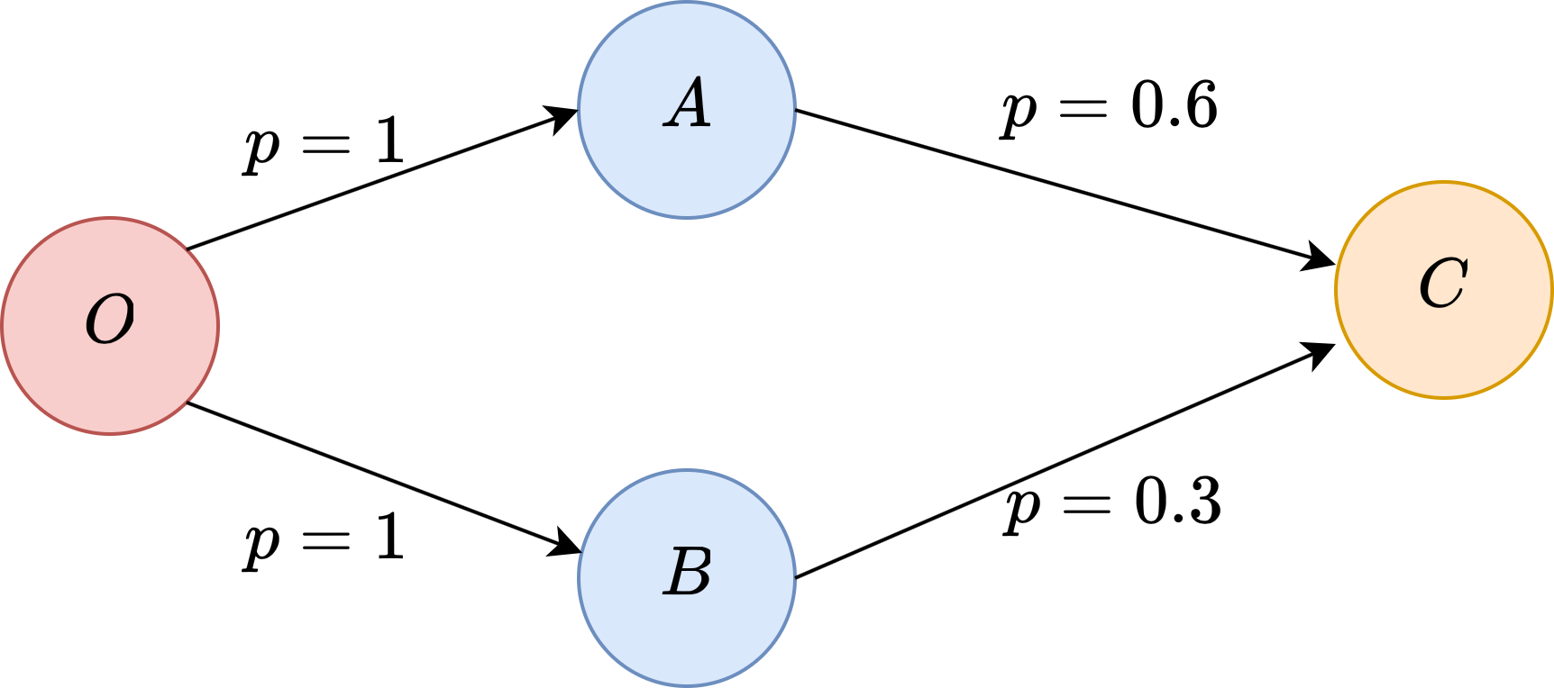
  To illustrate this, we consider a simple directed graph consisting of four nodes, $O,A,B$, and $C$, and four directed edges $(O,A),(O,B),(A,C)$, and $(A,B)$ shown in Figure 1, with $p_{O,A}=p_{O,B}=1,p_{A,C}=0.6$, and $p_{B,C}=0.3$. When node $O$ is selected as the seed set, nodes $O$ and $A$ would always be activated simultaneously at time step $t=1$. Subsequently, $A,B$ would attempt to influence their inactive neighbor $C$, with probability $p_{A,C}=0.6$ and $p_{B,C}=0.3$, respectively. Notably, under node-level feedback, only the combined effect of both $A$ and $B$ rather than the realizations on each edges $(A,C)$ and $(B,C)$ are observed. Suppose we were to apply classical UCB-type approaches to design online algorithms. Optimistic estimators are required for each edge. Nevertheless, using node-level information alone, the optimistic estimators could only be improved to their true aggregated probability, $u_{A,C}=u_{B,C}=0.72$, even with infinite observations. These bounds are far from the true individual influence probabilities. Without better knowledge of the optimistic estimators, the selected seed set will not necessarily improve, making UCB approaches inapplicable. For this reason, we need to design alternative algorithms to overcome this issue significantly.

• •

  The second challenge is the unknown distribution of $\rho_{n}^{*}$ involved in the confidence region established by Theorem 3.1. Recall that $\rho_{n}^{*}$ is the optimal solution to Prob.(6). In particular, we have $\rho_{n}^{*}=\max\{\rho|\mathbf{V}_{n}-\rho\mathbf{M}_{n}\succeq 0\}$ and $\mathbf{M}_{n}\succeq\mathbf{V}_{n}\succeq\rho_{n}^{*}\mathbf{M}_{n}$. Clearly, as both $\mathbf{V}_{n}$ and $\mathbf{M}_{n}$ are positive semi-definite matrices, $\rho_{n}^{*}\geq 0$ always holds. However, the trivial solution $\rho_{n}^{*}=0$ to (6) does not shed light on the relationship between $\mathbf{V}_{n}$ and $\mathbf{M}_{n}$. Moreover, let $\mathcal{C}_{n}$ be the confidence region constructed in (8), as the radius of this ellipsoid is proportional to $1/\rho_{n}^{*}$, we must investigate the distribution of $\rho_{n}^{*}$ to ensure the boundedness of the confidence region.

• •

  Third, the confidence region $\mathcal{C}_{n}$ (8) is constructed using feature information from activated hyper-edges, in particular, $\mathbf{V}_{n}$, instead of the full information matrix $\mathbf{M}_{n}$. Existing approaches in the bandits literature can only analyze the regret when we build up the confidence region $\mathcal{C}_{n}$ using the full information matrix $\mathbf{M}_{n}$ instead of $\mathbf{V}_{n}$. It remains unclear how to investigate the performance of the online algorithm in the latter scenario.

These challenges mentioned above make node-level IC learning highly nontrivial. To address these issues, we develop a novel learning algorithm that consists of exploration and exploitation phases and study its theoretical performance.

Recall the Maximum Likelihood Estimation in Section 3, for each edge $e=(u,v)\in\mathcal{E}$ with activation probability $p_{u,v}$, by taking the log-transformation $x_{u,v}^{\top}\theta^{*}=-\log(1-p_{u,v})$, the activation probability on each edge can be expressed as $p_{u,v}=1-\exp(-x_{u,v}^{\top}\theta^{*})$. Also, we define $p(\theta)$ as the collection of influence probabilities under parameter $\theta$ such that $p_{e}(\theta)=1-\exp(x_{e}^{\top}\theta)$ for all $e\in\mathcal{E}$. In particular, we have the true influence probability $p_{e}=p_{e}(\theta^{*})$.

References

- Abbasi-Yadkori et al. (2011) Abbasi-Yadkori Y, Pál D, Szepesvári C (2011) Improved algorithms for linear stochastic bandits. Advances in Neural Information Processing Systems, 2312–2320.
- Agrawal et al. (2017) Agrawal S, Avadhanula V, Goyal V, Zeevi A (2017) Thompson sampling for the mnl-bandit. Conference on Learning Theory, 76–78 (PMLR).
- Agrawal et al. (2019) Agrawal S, Avadhanula V, Goyal V, Zeevi A (2019) Mnl-bandit: A dynamic learning approach to assortment selection. Operations Research 67(5):1453–1485.
- Audibert et al. (2014) Audibert JY, Bubeck S, Lugosi G (2014) Regret in online combinatorial optimization. Mathematics of Operations Research 39(1):31–45.
- Bharathi et al. (2007) Bharathi S, Kempe D, Salek M (2007) Competitive influence maximization in social networks. Proceedings of the 3rd International Conference on Internet and Network Economics, 306–311, WINE’07 (Berlin, Heidelberg: Springer-Verlag), ISBN 3540771042.
- Chen et al. (2020) Chen N, Li A, Yang S (2020) Revenue maximization and learning in products ranking. arXiv preprint arXiv:2012.03800 .
- Chen et al. (2016a) Chen W, Lin T, Tan Z, Zhao M, Zhou X (2016a) Robust influence maximization. Proceedings of the 22nd ACM SIGKDD International Conference on Knowledge Discovery and Data Mining, 795–804, KDD ’16 (New York, NY, USA: Association for Computing Machinery), ISBN 9781450342322.
- Chen et al. (2013) Chen W, Wang Y, Yuan Y (2013) Combinatorial multi-armed bandit: General framework and applications. International Conference on Machine Learning, 151–159 (PMLR).
- Chen et al. (2016b) Chen W, Wang Y, Yuan Y, Wang Q (2016b) Combinatorial multi-armed bandit and its extension to probabilistically triggered arms. The Journal of Machine Learning Research 17(1):1746–1778.
- Cheung et al. (2019) Cheung WC, Tan V, Zhong Z (2019) A thompson sampling algorithm for cascading bandits. The 22nd International Conference on Artificial Intelligence and Statistics, 438–447.
- Combes et al. (2015) Combes R, Talebi MS, Proutiere A, Lelarge M (2015) Combinatorial bandits revisited. Proceedings of the 28th International Conference on Neural Information Processing Systems - Volume 2, 2116–2124, NIPS’15 (Cambridge, MA, USA: MIT Press).
- Fisher (1997) Fisher R (1997) On an absolute criterion for fitting frequency curves.
- Gai et al. (2012) Gai Y, Krishnamachari B, Jain R (2012) Combinatorial network optimization with unknown variables: Multi-armed bandits with linear rewards and individual observations. IEEE/ACM Transactions on Networking 20(5):1466–1478.
- Goyal et al. (2010) Goyal A, Bonchi F, Lakshmanan LV (2010) Learning influence probabilities in social networks. Proceedings of the third ACM international conference on Web search and data mining, 241–250 (ACM).
- He and Kempe (2016) He X, Kempe D (2016) Robust influence maximization. Proceedings of the 22nd ACM SIGKDD International Conference on Knowledge Discovery and Data Mining .
- He and Kempe (2018) He X, Kempe D (2018) Stability and robustness in influence maximization 12(6), ISSN 1556-4681.
- Katariya et al. (2016) Katariya S, Kveton B, Szepesvari C, Wen Z (2016) Dcm bandits: Learning to rank with multiple clicks. International Conference on Machine Learning, 1215–1224.
- Kempe et al. (2003) Kempe D, Kleinberg J, Tardos É (2003) Maximizing the spread of influence through a social network. Proceedings of the ninth ACM SIGKDD international conference on Knowledge discovery and data mining, 137–146 (ACM).
- Kveton et al. (2015a) Kveton B, Szepesvari C, Wen Z, Ashkan A (2015a) Cascading bandits: Learning to rank in the cascade model. International Conference on Machine Learning, 767–776.
- Kveton et al. (2015b) Kveton B, Wen Z, Ashkan A, Szepesvari C (2015b) Combinatorial cascading bandits. Advances in Neural Information Processing Systems, 1450–1458.
- Kveton et al. (2015c) Kveton B, Wen Z, Ashkan A, Szepesvari C (2015c) Tight regret bounds for stochastic combinatorial semi-bandits. Artificial Intelligence and Statistics, 535–543 (PMLR).
- Lei et al. (2015) Lei S, Maniu S, Mo L, Cheng R, Senellart P (2015) Online influence maximization. Proceedings of the 21th ACM SIGKDD International Conference on Knowledge Discovery and Data Mining, 645–654, KDD ’15 (New York, NY, USA: ACM), ISBN 978-1-4503-3664-2.
- Li et al. (2017) Li L, Lu Y, Zhou D (2017) Provably optimal algorithms for generalized linear contextual bandits. Proceedings of the 34th International Conference on Machine Learning-Volume 70, 2071–2080 (JMLR. org).
- Li et al. (2020) Li S, Kong F, Tang K, Li Q, Chen W (2020) Online influence maximization under linear threshold model. Proceedings of the 33rd Conference on Neural Information Processing Systems (NeurIPS) .
- Mannor and Shamir (2011) Mannor S, Shamir O (2011) From bandits to experts: On the value of side-observations. Advances in Neural Information Processing Systems, volume 24.
- McCullagh (2019) McCullagh P (2019) Generalized linear models .
- Nemhauser et al. (1978) Nemhauser GL, Wolsey LA, Fisher ML (1978) An analysis of approximations for maximizing submodular set functions i. Mathematical Programming 14(1):265–294, ISSN 1436-4646.
- Netrapalli and Sanghavi (2012) Netrapalli P, Sanghavi S (2012) Learning the graph of epidemic cascades. ACM SIGMETRICS Performance Evaluation Review 40:211–222.
- Oh and Iyengar (2021) Oh Mh, Iyengar G (2021) Multinomial logit contextual bandits: Provable optimality and practicality. arXiv preprint arXiv:2103.13929 .
- Saito et al. (2008) Saito K, Nakano R, Kimura M (2008) Prediction of information diffusion probabilities for independent cascade model. International Conference on Knowledge-Dased and Intelligent Information and Engineering Systems, 67–75 (Springer).
- Tropp et al. (2015) Tropp JA, et al. (2015) An introduction to matrix concentration inequalities. Foundations and Trends® in Machine Learning 8(1-2):1–230.
- Valko (2016) Valko M (2016) Bandits on graphs and structures. Ph.D. thesis.
- Vaswani and Duttachoudhury (2013) Vaswani S, Duttachoudhury N (2013) Learning influence diffusion probabilities under the linear threshold model .
- Vaswani et al. (2015) Vaswani S, Lakshmanan L, Schmidt M, et al. (2015) Influence maximization with bandits. arXiv preprint arXiv:1503.00024 .
- Wang and Chen (2017) Wang Q, Chen W (2017) Improving regret bounds for combinatorial semi-bandits with probabilistically triggered arms and its applications. NIPS.
- Wen et al. (2017) Wen Z, Kveton B, Valko M, Vaswani S (2017) Online influence maximization under independent cascade model with semi-bandit feedback. Advances in Neural Information Processing Systems, 3022–3032.
- Wilkinson (1965) Wilkinson JH (1965) The algebraic eigenvalue problem, volume 662 (Oxford Clarendon).
- Yang et al. (2019) Yang S, Wang S, Truong VA (2019) Online learning and optimization under a new linear-threshold model with negative influence. arXiv preprint arXiv:1911.03276 .
- Zong et al. (2016) Zong S, Ni H, Sung K, Ke NR, Wen Z, Kveton B (2016) Cascading bandits for large-scale recommendation problems. Proceedings of the Thirty-Second Conference on Uncertainty in Artificial Intelligence, 835–844, UAI’16 (Arlington, Virginia, USA: AUAI Press), ISBN 9780996643115.
Appendix
Appendix A Proofs of Technical Lemmas
A.1 Proof of Lemma 4.1
Proof A.1
Proof. Denote by . The desired inequality can be equivalently expressed as