跳到论文正文
W Papers独立论文阅读器 arXiv:2109.02494 论文正文 计算阅读时间 · 0%
引用这篇论文根据当前论文元数据生成,正式投稿前建议核对。


License: CC BY 4.0
arXiv:2109.02494v4 [math.FA] 05 Oct 2023

Stable Gabor phase retrieval in Gaussian shift-invariant spaces via biorthogonality

Philipp Grohs*,†,‡ Address: *Faculty of Mathematics, University of Vienna, Oskar-Morgenstern-Platz 1, 1090 Vienna, Austria Address: †Research Network DataScience@UniVie, University of Vienna, Kolingasse 14-16, 1090 Vienna, Austria Address: ‡Johann Radon Institute of Applied and Computational Mathematics, Austrian Academy of Sciences, Altenbergstrasse 69, 4040 Linz, Austria Email address: philipp.grohs@univie.ac.at, philipp.grohs@oeaw.ac.at and Lukas Liehr* Email address: lukas.liehr@univie.ac.at
Abstract.

We study the phase reconstruction of signals ff belonging to complex Gaussian shift-invariant spaces V∞​(φ)V^{\infty}(\varphi) from spectrogram measurements |𝒢​f​(X)||\mathcal{G}f(X)| where 𝒢\mathcal{G} is the Gabor transform and X⊆ℝ2X\subseteq{\mathbb{R}}^{2}. An explicit reconstruction formula will demonstrate that such signals can be recovered from measurements located on parallel lines in the time-frequency plane by means of a Riesz basis expansion. Moreover, connectedness assumptions on |f||f| result in stability estimates in the situation where one aims to reconstruct ff on compact intervals. Driven by a recent observation that signals in Gaussian shift-invariant spaces are determined by lattice measurements [Grohs, P., Liehr, L., Injectivity of Gabor phase retrieval from lattice measurements, Appl. Comput. Harmon. Anal. 62 (2023), pp. 173–193] we prove a sampling result on the stable approximation from finitely many spectrogram samples. The resulting algorithm provides a provably stable and convergent approximation technique. In addition, it constitutes a method of approximating signals in function spaces beyond V∞​(φ)V^{\infty}(\varphi), such as Paley-Wiener spaces.

Keywords. phase retrieval, Gabor transform, shift-invariant spaces, dual generator, Riesz bases, signal analysis

AMS subject classifications. 42C15, 46B15, 94A12, 94A20

1. Introduction

Phaseless signal reconstruction deals with the problem of recovering a function ff from intensity measurements of the form {|A​f​(x)|:x∈X}\{|Af(x)|:x\in X\} where AA is a linear transformation and XX is a subset of the domain of A​fAf. This is known as the phase retrieval problem, a non-linear inverse problem arising in numerous applications in science and engineering, such as coherent diffraction imaging [13, 14, 31], speech recognition [5] and quantum mechanics [12]. In the situation where ff belongs to an infinite-dimensional Banach or Hilbert space, phase retrieval is known to be never uniformly stable [2, 6], hence constituting a challenging problem for numerical reconstruction approaches. See the surveys [15, 20] for a current overview on uniqueness, stability and algorithms for phase retrieval. Recent attention was drawn to signals having a shift-invariant structure, that is,

(1) f∈Vβp(ϕ)={∑n∈ℤcnϕ(⋅−βn):(cn)n∈ℓp(ℤ)},f\in V_{\beta}^{p}(\phi)=\left\{\sum_{n\in{\mathbb{Z}}}c_{n}\phi(\cdot-\beta n):(c_{n})_{n}\in\ell^{p}({\mathbb{Z}})\right\},

where ϕ∈Lp​(ℝ)\phi\in L^{p}({\mathbb{R}}) is the so-called generator of Vβp​(ϕ)V_{\beta}^{p}(\phi) and p∈[1,∞]p\in[1,\infty]. The constant β>0\beta>0 is a regularity parameter, commonly referred to as the step-size. In a series of papers, Chen et. al. studied the phase retrievability of a real-valued map ff from its modulus |f|,A=Id|f|,A=\mathrm{Id}, assuming that the generator has compact support [7, 8, 9]. Shenoy et. el. investigated the situation where A=ℱA={\mathcal{F}} is the Fourier transform and the defining sequence (cn)n(c_{n})_{n} of ff obeys special properties [32]. In the situation where ϕ=sinc\phi=\mathrm{sinc} is the cardinal sine, i.e. the considered signals lie in the classical Paley-Wiener space, Thakur demonstrated how to recover a real-valued band-limited function from unsigned samples lying on a suitable dense sampling set [33]. Similar results for real-valued maps were derived for Gaussian generators as well as totally positive generators of Gaussian type and are due to Gröchenig [19] and Romero [30]. Besides, it was shown that if ϕ=φσ\phi=\varphi^{\sigma} is the Gaussian

(2) φσ​(t)=e−t22​σ2\varphi^{\sigma}(t)=e^{-\frac{t^{2}}{2\sigma^{2}}}

with variance σ2\sigma^{2} then, in general, complex-valued maps are not determined from samples of their absolute value. Hence, additional information is needed to achieve injectivity for complex signals from measurements |A​f||Af| with a suitably chosen signal-transformation AA. The authors of the present article proved in [22] that every complex-valued map in Vβ1​(φ)V_{\beta}^{1}(\varphi) is uniquely determined up to a global phase factor from measurements of the form |𝒱g​f​(X)||\mathcal{V}_{g}f(X)| where 𝒱g\mathcal{V}_{g} is the short-time Fourier transform with Gaussian window g=φσg=\varphi^{\sigma},

(3) 𝒱g​f​(x,ω)=∫ℝf⁡(t)​g⁡(t−x)¯​e−2​π​i​ω​t​𝑑t,\mathcal{V}_{g}f(x,\omega)=\int_{\mathbb{R}}f(t)\overline{g(t-x)}e^{-2\pi i\omega t}\,dt,

and X⊂ℝ2X\subset{\mathbb{R}}^{2} is a separated set of sampling points in the time-frequency plane. The resulting phase retrieval problem with transformation A=𝒱gA=\mathcal{V}_{g} is known as the Gabor phase retrieval problem which plays an important role in applications such as ptychography, a popular and highly successful approach in coherent diffraction imaging. The previous observations serve as the starting point for a more penetrating investigation of the Gabor phase retrieval problem in a Gaussian shift-invariant setting and motivate the work in hand. In particular, we derive an explicit inversion formula and stability estimates as well as propose a new reconstruction algorithm which approximates complex-valued signals in Vβ∞​(φ)V_{\beta}^{\infty}(\varphi) from finitely many (deterministic) samples of |𝒱g​f||\mathcal{V}_{g}f| in a provable and stable manner.

Classical algorithmic approaches on solving the phase retrieval problem are based on fixed point iterations, iterative projection methods and gradient descent methods. Examples include the alternating projection method, the Gerchberg–Saxton algorithm [18], error reduction [17], the Douglas-Rachford algorithm [16], Hybrid Input-Output Algorithm [17] and the Averaged Alternating Reflection Algorithm [29, 28]. The difficulty of analyzing convergence and robustness of these methods lies in the non-convexity of the phase retrieval problem. Heuristically, these methods perform well if one chooses a right initialization which is close to a solution of the problem. However, it is in general unclear how to perform the initialization step and provide convergent results in a noise regime. Moreover, the discretization of these methods in an infinite-dimensional setting constitutes a difficult task. In contrast, the derived algorithm of the present paper overcomes these difficulties by providing a provably convergent approximation routine from noisy samples. Moreover, we quantify exactly how many samples of |𝒱g​f||\mathcal{V}_{g}f| need to be taken in order to guarantee a given reconstruction error.

1.1. Notation

Throughout this article, the shift-invariant space Vβp​(ϕ)V_{\beta}^{p}(\phi), the Gaussian φσ\varphi^{\sigma} and the short-time Fourier transform are defined as in (1), (2) and (3), respectively. The cross-ambiguity function of ff and gg is the map A⁡(f,g)​(x,ω)=eπ​i​x​ω​𝒱g​f​(x,ω)A(f,g)(x,\omega)=e^{\pi ix\omega}\mathcal{V}_{g}f(x,\omega). The spectrogram of ff w.r.t. to a window gg is given by the map (x,ω)↦|𝒱g​f​(x,ω)|2(x,\omega)\mapsto|\mathcal{V}_{g}f(x,\omega)|^{2}. If g=φσg=\varphi^{\sigma} is a Gaussian then we set

𝒢≔𝒱φ≔𝒱φσ\mathcal{G}\coloneqq\mathcal{V}_{\varphi}\coloneqq\mathcal{V}_{\varphi^{\sigma}}

and call 𝒢\mathcal{G} the Gabor transform of ff. For clarity of the exposition and simplicity of notation, we will drop the dependence on σ\sigma. For a function f:ℝ→ℂf:{\mathbb{R}}\to{\mathbb{C}} and an ω∈ℝ\omega\in{\mathbb{R}} we define its tensor product fωf_{\omega} via

(4) fω≔(Tω​f)​f¯f_{\omega}\coloneqq(T_{\omega}f)\overline{f}

where Tωf=f(⋅−ω)T_{\omega}f=f(\cdot-\omega) is the shift-operator. Moreover, the modulation operator MωM_{\omega} is defined by Mω​f​(t)=e2​π​i​ω​t​f​(t)M_{\omega}f(t)=e^{2\pi i\omega t}f(t). In Section 2 we will exhibit that under suitable assumptions on ϕ\phi the system of translates (Tβ​n​ϕ)n∈ℤ(T_{\beta n}\phi)_{n\in{\mathbb{Z}}} forms a Riesz basis for the space Vβ2​(ϕ)V_{\beta}^{2}(\phi). Denoting by SS the frame operator associated with (Tβ​n​ϕ)n∈ℤ(T_{\beta n}\phi)_{n\in{\mathbb{Z}}} and making use of the property that the operators SS and Tβ​nT_{\beta n} commute for every n∈ℤn\in{\mathbb{Z}} implies that there exists a map ϕ~\tilde{\phi} such that (Tβ​n​ϕ~)n∈ℤ(T_{\beta n}\tilde{\phi})_{n\in{\mathbb{Z}}} is the dual frame of (Tβ​n​ϕ)n∈ℤ(T_{\beta n}\phi)_{n\in{\mathbb{Z}}}. The function ϕ~\tilde{\phi} given by

(5) ϕ~≔S−1​ϕ\tilde{\phi}\coloneqq S^{-1}\phi

is called the dual generator of ϕ\phi. If (Tβ​n​ϕ)n∈ℤ(T_{\beta n}\phi)_{n\in{\mathbb{Z}}} forms a Riesz basis for Vβ2​(ϕ)V_{\beta}^{2}(\phi) and f=∑ncn​Tβ​n​ϕf=\sum_{n}c_{n}T_{\beta n}\phi then we call c=(cn)n⊂ℂc=(c_{n})_{n}\subset{\mathbb{C}} the defining sequence of ff. In order to study stability properties of the Gabor phase retrieval problem in a Gaussian shift-invariant regime we define a mixed norm as follow. Let α>0,p∈[1,∞]\alpha>0,p\in[1,\infty] and suppose that F:α​ℤ×ℝ→ℂF:\alpha{\mathbb{Z}}\times{\mathbb{R}}\to{\mathbb{C}} is measurable. The mixed norm ∥⋅∥α,p\|\cdot\|_{\alpha,p} is defined by

(6) ‖F‖α,p≔{(∑n∈ℤ‖F⁡(α​n,⋅)‖L1​(ℝ)p)1p,p∈[1,∞)supn∈ℤ‖F⁡(α​n,⋅)‖L1​(ℝ),p=∞.\|F\|_{\alpha,p}\coloneqq\begin{cases}\left(\sum_{n\in{\mathbb{Z}}}\|F(\alpha n,\cdot)\|_{L^{1}({\mathbb{R}})}^{p}\right)^{\tfrac{1}{p}},&p\in[1,\infty)\\ \sup_{n\in{\mathbb{Z}}}\|F(\alpha n,\cdot)\|_{L^{1}({\mathbb{R}})},&p=\infty\end{cases}.

This is the ℓp\ell^{p}-norm of the sequence (‖F⁡(α​n,⋅)‖L1​(ℝ))n∈ℤ(\|F(\alpha n,\cdot)\|_{L^{1}({\mathbb{R}})})_{n\in{\mathbb{Z}}}. If FF is defined on ℝ2{\mathbb{R}}^{2} we set ‖F‖α,p≔‖F|α​ℤ×ℝ‖α,p\|F\|_{\alpha,p}\coloneqq\|F|_{\alpha{\mathbb{Z}}\times{\mathbb{R}}}\|_{\alpha,p} where F|α​ℤ×ℝF|_{\alpha{\mathbb{Z}}\times{\mathbb{R}}} is the restriction of FF to α​ℤ×ℝ\alpha{\mathbb{Z}}\times{\mathbb{R}}. If not specified otherwise, all indices will run over the integers ℤ{\mathbb{Z}}. Finally, we say that two functions f,h:ℝ→ℂf,h:{\mathbb{R}}\to{\mathbb{C}} equal up to a global phase (or: up to a unimodular constant) if there exists a τ∈𝕋≔{z∈ℂ:|z|=1}\tau\in{\mathbb{T}}\coloneqq\{z\in{\mathbb{C}}:|z|=1\} such that f=τ​hf=\tau h.

1.2. Main results

The first main result, Theorem 1.1, provides an explicit inversion formula of a function f∈Vβ∞​(φ)f\in V_{\beta}^{\infty}(\varphi) from its spectrogram |𝒢​f​(X)||\mathcal{G}f(X)| where X=β2​ℤ×ℝX=\frac{\beta}{2}{\mathbb{Z}}\times{\mathbb{R}} is a set of vertical lines in the time-frequency plane.

Theorem 1.1.

Let f∈Vβ∞​(φ)f\in V_{\beta}^{\infty}(\varphi) and let p∈ℝp\in{\mathbb{R}} such that f⁡(p)≠0f(p)\neq 0. Then there exists a unimodular constant τ∈𝕋\tau\in{\mathbb{T}} such that

f⁡(p+ω)=τ​C−12​∑n∈ℤ(∫ℝ|𝒢​f​(β2​n,t)|2​e2​π​i​ω​t​𝑑t)​Tβ2​n​φω~​(p+ω)f(p+\omega)=\tau C^{-\frac{1}{2}}\sum_{n\in{\mathbb{Z}}}\left(\int_{\mathbb{R}}|\mathcal{G}f(\tfrac{\beta}{2}n,t)|^{2}e^{2\pi i\omega t}\,dt\right)T_{\frac{\beta}{2}n}\widetilde{\varphi_{\omega}}(p+\omega)

for every ω∈ℝ\omega\in{\mathbb{R}} where C=∑n∈ℤ(∫ℝ|𝒢​f​(β2​n,t)|2​𝑑t)​Tβ2​n​φ0~​(p)C=\sum_{n\in{\mathbb{Z}}}\left(\int_{\mathbb{R}}|\mathcal{G}f(\tfrac{\beta}{2}n,t)|^{2}\,dt\right)T_{\frac{\beta}{2}n}\widetilde{\varphi_{0}}(p) and φω~\widetilde{\varphi_{\omega}} is the dual generator of the Gaussian tensor product φω\varphi_{\omega}.

In the previous theorem the maps {φω~:ω∈ℝ}\{\widetilde{\varphi_{\omega}}:\omega\in{\mathbb{R}}\} constitute a parametrized system of dual generators. In particular, the statement shows that two functions f,h∈Vβ∞​(φ)f,h\in V_{\beta}^{\infty}(\varphi) agree up a global phase provided that their spectrograms agree on X=β2​ℤ×ℝX=\frac{\beta}{2}{\mathbb{Z}}\times{\mathbb{R}}. Note, that this is a uniqueness statement within the signal class Vβ∞​(φ)V_{\beta}^{\infty}(\varphi). A similar statement does not hold if one replaces Vβ∞​(φ)V_{\beta}^{\infty}(\varphi) by L2​(ℝ){L^{2}({\mathbb{R}})}, as we have shown in [21].

Next, we study stability properties of the above inversion. Heuristically, Theorem 1.2 assumes that the map ff has the property that |f||f| is not too small on large intervals. More precisely, it will be assumed that there exists J∈ℕ,p1,…,pJ∈ℝJ\in{\mathbb{N}},p_{1},\dots,p_{J}\in{\mathbb{R}} and γ>0\gamma>0 such that

J≥2∧p1<p2<⋯<pJ∧|f⁡(pj)|≥γ​∀j∈{1,…,J}.J\geq 2\ \ \land\ \ p_{1}<p_{2}<\cdots<p_{J}\ \ \land\ \ |f(p_{j})|\geq\gamma\ \forall j\in\{1,\dots,J\}.

Condition (P) excludes examples of the form fs+=φ(⋅−a)+φ(⋅−b),fs−=φ(⋅−a)−φ(⋅−b),s=|a−b|f^{+}_{s}=\varphi(\cdot-a)+\varphi(\cdot-b),f^{-}_{s}=\varphi(\cdot-a)-\varphi(\cdot-b),s=|a-b|, where it is known that exponential instabilities arise for growing ss [3]. These examples further show that an assumption on |f||f| of the above form cannot be dropped.

Theorem 1.2.

Let γ>0\gamma>0, f∈Vβ∞​(φ)f\in V_{\beta}^{\infty}(\varphi) and p1<⋯<pJ∈ℝp_{1}<\cdots<p_{J}\in{\mathbb{R}} such that |f⁡(pj)|≥γ|f(p_{j})|\geq\gamma for all jj. If I=[p1−r,pJ+r]I=[p_{1}-r,p_{J}+r] and r=max1≤j≤J−1⁡(pj+1−pj)r=\max_{1\leq j\leq J-1}(p_{j+1}-p_{j}) then for every g∈Vβ∞​(φ)g\in V_{\beta}^{\infty}(\varphi) we have

minτ∈𝕋⁡‖f−τ​g‖L∞​(I)≲β,σ(J−1)er24​σ2max⁡{‖f‖L∞​(I)2,‖f‖L∞​(I)+‖g‖L∞​(I)}min⁡{γ,γ3}∥|𝒢f|2−|𝒢g|2∥β2,∞\begin{split}&\min_{\tau\in{\mathbb{T}}}\|f-\tau g\|_{L^{\infty}(I)}\\ &\lesssim_{\beta,\sigma}(J-1)e^{\frac{r^{2}}{4\sigma^{2}}}\frac{\max\{\|f\|_{L^{\infty}(I)}^{2},\|f\|_{L^{\infty}(I)}+\|g\|_{L^{\infty}(I)}\}}{\min\{\gamma,\gamma^{3}\}}\||\mathcal{G}f|^{2}-|\mathcal{G}g|^{2}\|_{\frac{\beta}{2},\infty}\end{split}

and the implicit constant depends only on the step-size β\beta and the standard-deviation σ\sigma of the Gaussian φ=φσ\varphi=\varphi^{\sigma}.

Refer to caption
Figure 1. Visualization of condition (P): the points p1,…,p9p_{1},\dots,p_{9} satisfy the properties |f⁡(pj)|≥γ|f(p_{j})|\geq\gamma for all j=1,…,9j=1,\dots,9 and pj+1−pj≤rp_{j+1}-p_{j}\leq r for all j=1,…,8j=1,\dots,8.

We seek to discretize the previous regime in the sense that it yields an algorithmic approximation of functions in Vβ∞​(φ)V_{\beta}^{\infty}(\varphi) from finitely many measurements located on a grid of the form

(7) X=β2​{−N,…,N}×h⁡{−H,…,H}X=\tfrac{\beta}{2}\{-N,\dots,N\}\times h\{-H,\dots,H\}

where N,H∈ℕ,h,β>0N,H\in{\mathbb{N}},h,\beta>0 rather than X=β2​ℤ×ℝX=\frac{\beta}{2}{\mathbb{Z}}\times{\mathbb{R}}. If η∈ℝ(2​N+1)×(2​H+1)\eta\in{\mathbb{R}}^{(2N+1)\times(2H+1)} denotes a noise matrix then the given samples 𝔖\mathfrak{S} take the form

𝔖=(|𝒢​f​(X)|2+ηn,k)n,k∈ℝ(2​N+1)×(2​H+1),𝔖⁡(n,k)=|𝒢​f​(β2​n,h​k)|2+ηn,k.\begin{split}&\mathfrak{S}=(|\mathcal{G}f(X)|^{2}+\eta_{n,k})_{n,k}\in{\mathbb{R}}^{(2N+1)\times(2H+1)},\\ &\mathfrak{S}(n,k)=|\mathcal{G}f(\tfrac{\beta}{2}n,hk)|^{2}+\eta_{n,k}.\end{split}

The contribution of the noise η\eta will be quantified in terms of the ℓ∞\ell^{\infty}-operator norm of η\eta, i.e. the maximum absolute row sum of η\eta. We denote this norm by ‖η‖∞\|\eta\|_{\infty}. The so-called numerical approximation routine ℛ\mathcal{R} depends only on 𝔖\mathfrak{S} and is defined as follows: for p1<p2<⋯<pJp_{1}<p_{2}<\cdots<p_{J} define constants cjc_{j} by cj=h​∑n∑k𝔖⁡(n,k)​Tβ2​n​φ0~​(pj),c_{j}=h\sum_{n}\sum_{k}\mathfrak{S}(n,k)T_{\frac{\beta}{2}n}\widetilde{\varphi_{0}}(p_{j}), functions LjL_{j} by

Lj​(ω)=hcj​∑n∑k𝔖⁡(n,k)​e2​π​i​ω​h​k​Tβ2​n​φω~​(pj+ω)L_{j}(\omega)=\frac{h}{\sqrt{c_{j}}}\sum_{n}\sum_{k}\mathfrak{S}(n,k)e^{2\pi i\omega hk}T_{\frac{\beta}{2}n}\widetilde{\varphi_{\omega}}(p_{j}+\omega)

and phases ν0,…,νJ−1∈𝕋\nu_{0},\dots,\nu_{J-1}\in{\mathbb{T}} by

ν0=1,νj=Lj​(pj+1−pj)|Lj​(pj+1−pj)|​(j=1,…,J−1).\nu_{0}=1,\ \ \nu_{j}=\frac{L_{j}(p_{j+1}-p_{j})}{|L_{j}(p_{j+1}-p_{j})|}\ (j=1,\dots,J-1).

Assuming that LjL_{j} and νj\nu_{j} are well-defined, i.e. cj>0c_{j}>0 and Lj​(pj+1−pj)≠0L_{j}(p_{j+1}-p_{j})\neq 0 we define ℛ:[p1,pJ]→ℂ\mathcal{R}:[p_{1},p_{J}]\to{\mathbb{C}} by

(8) ℛ(t)=ν1⋯νj−1Lj(ω),\mathcal{R}(t)=\nu_{1}\cdots\nu_{j-1}L_{j}(\omega),

if t∈[p1,pJ]t\in[p_{1},p_{J}] such that t∈(pj,pj+1]t\in(p_{j},p_{j+1}] with t=pj+ωt=p_{j}+\omega. For t=p1t=p_{1} we define ℛ​(t)=L1​(0)\mathcal{R}(t)=L_{1}(0). This function has the property that it approximates ff from finitely many noisy samples. Figure 2 illustrates the reconstruction performance of the numerical reconstruction routine ℛ\mathcal{R} applied to finitely many noisy spectrogram samples of a complex-valued signal. The following theorem proves stability and convergence of this algorithm.

Theorem 1.3.

Suppose that f∈Vβ∞​(φ)f\in V_{\beta}^{\infty}(\varphi) has defining sequence c∈ℓ∞​(ℤ)c\in\ell^{\infty}({\mathbb{Z}}) and that there exist

−s≕p1<p2<⋯<pJ≔s-s\eqqcolon p_{1}<p_{2}<\cdots<p_{J}\coloneqq s

with |f⁡(pj)|≥γ|f(p_{j})|\geq\gamma and max1≤j≤J−1⁡(pj+1−pj)≤r\max_{1\leq j\leq J-1}(p_{j+1}-p_{j})\leq r. Let I=[−s,s]I=[-s,s] and let 0<ε≤min⁡{γ22​8,γ34​‖f‖L∞​(I)}0<\varepsilon\leq\min\left\{\frac{\gamma^{2}}{2\sqrt{8}},\frac{\gamma^{3}}{4\|f\|_{L^{\infty}(I)}}\right\} and assume that the parameters h,H,Nh,H,N of the grid XX have the property that

1h≳σ,β,rlog(J​‖c‖∞2ε+1),N≳σ,β,rs+log(J​‖c‖∞2ε),\frac{1}{h}\gtrsim_{\sigma,\beta,r}\log\left(\frac{J\|c\|_{\infty}^{2}}{\varepsilon}+1\right),\ N\gtrsim_{\sigma,\beta,r}s+\log\left(\frac{J\|c\|_{\infty}^{2}}{\varepsilon}\right),
H≳σ,β,r1h(log(J​‖c‖∞2ε))1/2.\ H\gtrsim_{\sigma,\beta,r}\frac{1}{h}\left(\log\left(\frac{J\|c\|_{\infty}^{2}}{\varepsilon}\right)\right)^{1/2}.

If the noise level satisfies ∥η∥∞≲σ,β,rεh​J\|\eta\|_{\infty}\lesssim_{\sigma,\beta,r}\frac{\varepsilon}{hJ} then

(9) minτ∈𝕋⁡‖f−τ​ℛ‖L∞​(I)≤32​max⁡{1,‖f‖L∞​(I)2}min⁡{γ,γ5}​(ε+ε2).\min_{\tau\in{\mathbb{T}}}\|f-\tau\mathcal{R}\|_{L^{\infty}(I)}\leq 32\frac{\max\{1,\|f\|^{2}_{L^{\infty}(I)}\}}{\min\{\gamma,\gamma^{5}\}}(\varepsilon+\varepsilon^{2}).

The numerical approximation routine ℛ\mathcal{R} combined with Theorem 1.3 results in a provably stable and convergent approximation algorithm as soon as condition (P) is satisfied. Note that this is an assumption on |f||f| which is a-priori unknown if only samples of |𝒢​f||\mathcal{G}f| are available. However, this information is encoded in the spectrogram of ff: we will show that the modulus |f||f| of any f∈Vβ∞​(φ)f\in V_{\beta}^{\infty}(\varphi) can be approximated in a uniformly and globally stable way without imposing any additional assumption on ff, see the discussion following Corollary 3.7, as well as Lemma 3.8. Based on a reconstruction of |f||f| the resulting algorithm presented in Section 4 first detects points p1,…,pJp_{1},\dots,p_{J} such that condition (P) is satisfied and finally uses the numerical approximation routine ℛ\mathcal{R} to provide a reconstruction of ff. In this way, the information on the location of points pjp_{j} can be omitted.

Finally, we study the growth behavior of the number of spectrogram samples needed to approximate a function on an interval [−s,s][-s,s]. Assume that ff has the property that there exists a partition ⋯<p−1<p0<p1<⋯\cdots<p_{-1}<p_{0}<p_{1}<\cdots of the real line such that |f⁡(pj)|≥γ|f(p_{j})|\geq\gamma for some γ>0\gamma>0 and all j∈ℤj\in{\mathbb{Z}}. Suppose we aim to approximate ff on the interval [−s,s][-s,s] using the numerical approximation routine ℛ=ℛ⁡(s)\mathcal{R}=\mathcal{R}(s). How does the minimal number of spectrogram samples 𝒩⁡(s)\mathcal{N}(s) grow so that ℛ⁡(s)\mathcal{R}(s) achieves the bound (9) for a fixed ε>0\varepsilon>0?

Theorem 1.4.

Let ⋯<p−1<p0<p1<⋯\cdots<p_{-1}<p_{0}<p_{1}<\cdots be a partition of the real line such that supj∈ℤ(pj+1−pj)<∞\sup_{j\in{\mathbb{Z}}}(p_{j+1}-p_{j})<\infty. Let γ>0\gamma>0 and f∈Vβ∞​(φ)f\in V_{\beta}^{\infty}(\varphi) such that |f⁡(pj)|≥γ|f(p_{j})|\geq\gamma for all j∈ℤj\in{\mathbb{Z}}. Assume that the spectrogram samples 𝔖\mathfrak{S} are noiseless, η=0\eta=0, and ε\varepsilon is given as in Theorem 1.3. Then the minimal number of spectrogram samples 𝒩⁡(s)\mathcal{N}(s) needed to achieve the bound (9) on the interval [−s,s][-s,s] using the numerical approximation routine ℛ\mathcal{R} satisfies

𝒩(s)≲σ,βlog(s​‖c‖∞2ε)32(s+log(s​‖c‖∞2ε)).\mathcal{N}(s)\lesssim_{\sigma,\beta}\log\left(\frac{s\|c\|_{\infty}^{2}}{\varepsilon}\right)^{\frac{3}{2}}\left(s+\log\left(\frac{s\|c\|_{\infty}^{2}}{\varepsilon}\right)\right).

Theorems 1.1, 1.2, 1.3 and 1.4 are a direct consequence of Theorems 3.6, 3.10, 4.6 and Corollary 4.7 that will be proved in Sections 3.1, 3.2, 4.2 and 4.2, respectively.

Figure 2. Reconstruction of a complex-valued function f∈Vβ∞​(φ)f\in V_{\beta}^{\infty}(\varphi) (β=1,φ⁡(t)=e−π​t2\beta=1,\varphi(t)=e^{-\pi t^{2}}) on the interval [−16,16][-16,16] using the numerical approximation routine ℛ\mathcal{R} with spectrogram samples located at X=12​{−40,…,40}×112​{−60,…,60}X=\tfrac{1}{2}\{-40,\dots,40\}\times\tfrac{1}{12}\{-60,\dots,60\}. To each spectrogram sample, Gaussian noise with mean zero and standard deviation 0.001 is added, i.e. the measurement matrix 𝔖\mathfrak{S} takes the form 𝔖=|𝒢​f​(X)|2+𝒩⁡(0,σ2),σ=0.001\mathfrak{S}=|\mathcal{G}f(X)|^{2}+\mathcal{N}(0,\sigma^{2}),\sigma=0.001.

1.3. Outline

The article is structured as follows: in Section 2 we present the necessary general theory on shift-invariant spaces which will be used throughout the article. Section 3 starts with an abstract discussion on the reconstruction of arbitrary maps from their tensor product. These ideas will be applied to Gaussian shift-invariant spaces and lead to an explicit inversion formula from spectrogram measurements which makes use of a biorthogonal expansion. The section ends with a stability analysis of the derived reconstruction formula. In the final section, Section 4, we present and analyze an algorithmic way of approximating functions in Gaussian shift-invariant spaces from finitely many spectrogram samples. Moreover, we elaborate that the obtained algorithm approximates signals in Paley-Wiener spaces.

2. Preliminaries on shift-invariant spaces

2.1. General theory

For β>0,p∈[1,∞]\beta>0,p\in[1,\infty] and ϕ∈Lp​(ℝ)\phi\in L^{p}({\mathbb{R}}) let the shift-invariant space Vβp​(ϕ)V_{\beta}^{p}(\phi) be defined as in (1). Recall that a sequence (fn)n⊂ℋ(f_{n})_{n}\subset\mathcal{H} in a separable Hilbert space ℋ\mathcal{H} is said to be a Riesz basis for ℋ\mathcal{H} if it is complete in ℋ\mathcal{H} and there exist positive constants 0<A≤B0<A\leq B such that for arbitrary n∈ℕn\in{\mathbb{N}} and arbitrary c1,…,cn∈ℂc_{1},\dots,c_{n}\in{\mathbb{C}} one has

(10) A​∑j=1n|cj|2≤‖∑j=1ncj​fj‖2≤B​∑j=1n|cj|2.A\sum_{j=1}^{n}|c_{j}|^{2}\leq\left\|\sum_{j=1}^{n}c_{j}f_{j}\right\|^{2}\leq B\sum_{j=1}^{n}|c_{j}|^{2}.

The optimal constants AA and BB are called the lower and upper bound of (fn)n(f_{n})_{n}. Every Riesz basis with lower and upper bounds AA and BB is a frame with frame constants AA and BB. Associate to a Riesz basis (fn)n(f_{n})_{n} its frame operator S:ℋ→ℋS:\mathcal{H}\to\mathcal{H}, defined by S​f=∑n∈ℤ⟨f,fn⟩​fn.Sf=\sum_{n\in{\mathbb{Z}}}\langle f,f_{n}\rangle f_{n}. Then SS is a positive, invertible operator and (S−1​fn)n(S^{-1}f_{n})_{n} is biorthogonal to (fn)n(f_{n})_{n}, i.e.

⟨fn,S−1​fk⟩=δn​k≔{1n=k0n≠k.\langle f_{n},S^{-1}f_{k}\rangle=\delta_{nk}\coloneqq\begin{cases}1&n=k\\ 0&n\neq k\end{cases}.

Now let ℋ=Vβ2​(ϕ)\mathcal{H}=V_{\beta}^{2}(\phi) be a shift-invariant space with a square-integrable generator ϕ\phi. Define the 1-periodic map Φβ:ℝ→ℝ\Phi_{\beta}:{\mathbb{R}}\to{\mathbb{R}} via

(11) Φβ​(t)=∑n∈ℤ|ϕ^​(t+nβ)|2\Phi_{\beta}(t)=\sum_{n\in{\mathbb{Z}}}|\hat{\phi}(\tfrac{t+n}{\beta})|^{2}

where ϕ^=ℱ​ϕ\hat{\phi}={\mathcal{F}}\phi denotes the Fourier transform of ϕ\phi which is defined on L1​(ℝ)∩L2​(ℝ)L^{1}({\mathbb{R}})\cap{L^{2}({\mathbb{R}})} by

ϕ^​(ω)=ℱ​ϕ​(ω)=∫ℝϕ⁡(t)​e−2​π​i​ω​t​𝑑t\hat{\phi}(\omega)={\mathcal{F}}\phi(\omega)=\int_{\mathbb{R}}\phi(t)e^{-2\pi i\omega t}\,dt

and extends to a unitary operator on L2​(ℝ){L^{2}({\mathbb{R}})}. The map Φβ\Phi_{\beta} characterizes the property of (Tβ​n​ϕ)n(T_{\beta n}\phi)_{n} being a Riesz basis for Vβ2​(ϕ)V_{\beta}^{2}(\phi) [10, Theorem 9.2.5].

Theorem 2.1.

Let ϕ∈L2​(ℝ)\phi\in{L^{2}({\mathbb{R}})} and β>0\beta>0. Suppose that there exists 0<A≤B<∞0<A\leq B<\infty such that

(12) β​A≤Φβ​(t)≤β​B\beta A\leq\Phi_{\beta}(t)\leq\beta B

for almost every t∈[0,1]t\in[0,1]. Then Vβ2​(ϕ)V_{\beta}^{2}(\phi) is a closed subspace of L2​(ℝ)L^{2}({\mathbb{R}}) and (Tβ​n​ϕ)n(T_{\beta n}\phi)_{n} is a Riesz basis for Vβ2​(ϕ)V_{\beta}^{2}(\phi) with bounds AA and BB.

If ϕ\phi satisfies condition (12) and if S:Vβ2​(ϕ)→Vβ2​(ϕ)S:V_{\beta}^{2}(\phi)\to V_{\beta}^{2}(\phi) is the frame operator associated with (Tβ​n​ϕ)n(T_{\beta n}\phi)_{n} then SS commutes with β​ℤ\beta{\mathbb{Z}}-shifts, implying that (S−1​Tβ​n​ϕ)n=(Tβ​n​ϕ~)n(S^{-1}T_{\beta n}\phi)_{n}=(T_{\beta n}\tilde{\phi})_{n} with ϕ~=S−1​ϕ\tilde{\phi}=S^{-1}\phi [10, Lemma 9.4.1]. Accordingly, the canonical dual frame (S−1​Tβ​n​ϕ)n(S^{-1}T_{\beta n}\phi)_{n} has the same structure as (Tβ​n​ϕ)n(T_{\beta n}\phi)_{n}.

Definition 2.2.

Let β>0\beta>0 and ϕ∈L2​(ℝ)\phi\in{L^{2}({\mathbb{R}})} such that (Tβ​n​ϕ)n(T_{\beta n}\phi)_{n} is a Riesz basis for Vβ2​(ϕ)V_{\beta}^{2}(\phi). If SS is the frame operator associated with (Tβ​n​ϕ)n(T_{\beta n}\phi)_{n} then ϕ~≔S−1​ϕ\widetilde{\phi}\coloneqq S^{-1}\phi is called the dual generator of ϕ\phi.

Clearly, the dual generator generates the same shift-invariant space, i.e. Vβ2​(ϕ)=Vβ2​(ϕ~)V_{\beta}^{2}(\phi)=V_{\beta}^{2}(\widetilde{\phi}). In the situation of Theorem 2.1, the map ϕ~\widetilde{\phi} can be derived explicitly. To do so, define in a similar fashion as above the 1β\frac{1}{\beta}-periodization of |ϕ^|2|\hat{\phi}|^{2} as

Ψβ​(t)=∑n∈ℤ|ϕ^​(t+nβ)|2.\Psi_{\beta}(t)=\sum_{n\in{\mathbb{Z}}}|\hat{\phi}(t+\tfrac{n}{\beta})|^{2}.

The dual generator is then given as a formula of ϕ^\hat{\phi} and Ψ\Psi.

Theorem 2.3.

Suppose that (Tβ​n​ϕ)n(T_{\beta n}\phi)_{n} is a Riesz basis for Vβ2​(ϕ)V_{\beta}^{2}(\phi) with frame operator SS. Let D={t∈ℝ:Ψβ​(t)≠0}D=\{t\in{\mathbb{R}}:\Psi_{\beta}(t)\neq 0\} and let 𝟏D{\bm{1}}_{D} be the indicator function of DD. If the map θ\theta is defined as

θ⁡(ω)=β​ϕ^​(ω)Ψβ​(ω)​𝟏D​(ω)\theta(\omega)=\frac{\beta\hat{\phi}(\omega)}{\Psi_{\beta}(\omega)}{\bm{1}}_{D}(\omega)

then ϕ~≔ℱ−1​θ\tilde{\phi}\coloneqq{\mathcal{F}^{-1}}\theta is the dual generator of ϕ\phi.

Proof.

This follows from a generalization of [10, Proposition 9.4.2]. For the convenience of the reader, we provide a proof in the Appendix 5.1. ∎

Note that the structure of Vβ2​(ϕ)V_{\beta}^{2}(\phi) can be enriched by imposing further properties on the generator ϕ\phi. For instance, if ϕ\phi is continuous and belongs to the Wiener Amalgam space then Vβ2​(ϕ)V_{\beta}^{2}(\phi) is a reproducing kernel Hilbert space (RKHS). We refer to [4, 10, 11] for results in this direction.

2.2. Gaussian generators

We now specialize ϕ\phi to be the Gaussian φσ\varphi^{\sigma} with variance σ2\sigma^{2} as defined in Equation (2). For the sake of simplicity we write φ=φσ\varphi=\varphi^{\sigma} with the implicit understanding that φ\varphi has variance σ2\sigma^{2}. Properties of Vβ2​(φ)V_{\beta}^{2}(\varphi) can be expressed in terms of the Jacobi theta function of third kind. Recall that this is the map ϑ3:ℂ×(0,1)→ℂ\vartheta_{3}:{\mathbb{C}}\times(0,1)\to{\mathbb{C}},

ϑ3​(z,c)=∑n∈ℤcn2​e2​n​i​z.\vartheta_{3}(z,c)=\sum_{n\in{\mathbb{Z}}}c^{n^{2}}e^{2niz}.

For every fixed c∈(0,1)c\in(0,1), ϑ3\vartheta_{3} is an entire, π\pi-periodic map in zz. Using the results of the previous subsection gives

Corollary 2.4.

Let φ\varphi be a centred Gaussian with variance σ2\sigma^{2}. Then the 11-periodization of φ\varphi is given by

Φβ​(t)=σ​β​π​ϑ3​(π​t,φ⁡(β2)).\Phi_{\beta}(t)=\sigma\beta\sqrt{\pi}\vartheta_{3}(\pi t,\varphi(\tfrac{\beta}{\sqrt{2}})).

In particular, the system (Tβ​n​φ)n(T_{\beta n}\varphi)_{n} constitutes a Riesz basis for Vβ2​(φ)V_{\beta}^{2}(\varphi). Moreover, if the function Λ:ℝ→ℂ\Lambda:{\mathbb{R}}\to{\mathbb{C}} is defined as

Λ⁡(t)≔e−2​π2​σ2​t2ϑ3​(π​β​t,φ⁡(β2))\Lambda(t)\coloneqq\frac{e^{-2\pi^{2}\sigma^{2}t^{2}}}{\vartheta_{3}(\pi\beta t,\varphi(\frac{\beta}{\sqrt{2}}))}

then the dual-generator of φ\varphi is given by φ~=2​ℱ−1​Λ\widetilde{\varphi}=\sqrt{2}{\mathcal{F}^{-1}}\Lambda.

Proof.

The identity ℱ​φ​(t)=σ​2​π​e−2​π2​σ2​t2{\mathcal{F}}\varphi(t)=\sigma\sqrt{2\pi}e^{-2\pi^{2}\sigma^{2}t^{2}} implies that the 1-periodization Φβ\Phi_{\beta} is given by

(13) Φβ​(t)=2​π​σ2​∑ne−4​π2​σ2β2​(t+n)2=σ​β​π​∑ne−β2​n24​σ2​e2​π​i​n​t=σ​β​π​ϑ3​(π​t,φ⁡(β2)),\begin{split}\Phi_{\beta}(t)&=2\pi\sigma^{2}\sum_{n}e^{-\frac{4\pi^{2}\sigma^{2}}{\beta^{2}}(t+n)^{2}}=\sigma\beta\sqrt{\pi}\sum_{n}e^{-\frac{\beta^{2}n^{2}}{4\sigma^{2}}}e^{2\pi int}\\ &=\sigma\beta\sqrt{\pi}\vartheta_{3}(\pi t,\varphi(\tfrac{\beta}{\sqrt{2}})),\end{split}

where the second equality follows from Poisson’s summation formula. In a similar fashion, we obtain

(14) Ψβ​(t)=π​σ​β​ϑ3​(π​β​t,φ⁡(β2)),\Psi_{\beta}(t)=\sqrt{\pi}\sigma\beta\vartheta_{3}(\pi\beta t,\varphi(\tfrac{\beta}{\sqrt{2}})),

thereby proving the statement using Theorem 2.3. ∎

Figure 3. Dual generators of Gaussians φσ​(t)\varphi^{\sigma}(t) associated with the shift-invariant space Vβ2​(φ)V_{\beta}^{2}(\varphi) with step-sizes β=0.8,0.6,0.2\beta=0.8,0.6,0.2 and σ=β\sigma=\beta.

Note that the zeros of ϑ3\vartheta_{3} are bounded away from the real axis. Hence, the reciprocal theta function 1ϑ3\frac{1}{\vartheta_{3}} defines an analytic and periodic function in an open strip containing the real axis. It follows that the Fourier coefficients an=an​(c)a_{n}=a_{n}(c) of 1ϑ3\frac{1}{\vartheta_{3}} decay at least exponentially. If

(15) 1ϑ3​(π​β​t,c)=∑n∈ℤan​e2​π​i​β​n​t\frac{1}{\vartheta_{3}(\pi\beta t,c)}=\sum_{n\in{\mathbb{Z}}}a_{n}e^{2\pi i\beta nt}

with c=φ⁡(β2)c=\varphi(\tfrac{\beta}{\sqrt{2}}) then the identity ℱ⁡(s↦e−2​π2​σ2​s2)​(t)=(σ​2​π)−1​φ​(t){\mathcal{F}}(s\mapsto e^{-2\pi^{2}\sigma^{2}s^{2}})(t)=(\sigma\sqrt{2\pi})^{-1}\varphi(t) implies that φ~\widetilde{\varphi} can be written as

φ~​(t)=1σ​π​∑nan​T−β​n​φ​(t).\widetilde{\varphi}(t)=\frac{1}{\sigma\sqrt{\pi}}\sum_{n}a_{n}T_{-\beta n}\varphi(t).

Hence, up to a multiplicative constant, the defining sequence of the dual generator is given by the Fourier coefficients of the reciprocal theta function and therefore the decay of φ~\widetilde{\varphi} matches with the decay of (an)n(a_{n})_{n}. In fact, the Fourier coefficients of 1ϑ3\frac{1}{\vartheta_{3}} satisfy precisely an exponential decay (see a derivation by Janssen [27, p. 178] based on results of Whittaker and Watson [35, p. 489]): if the constant ξ=ξ⁡(c)\xi=\xi(c) is defined by

(16) ξ=∑n∈ℤ(−1)n​(2​n+1)​c(n+12)2\xi=\sum_{n\in\mathbb{Z}}(-1)^{n}(2n+1)c^{(n+\frac{1}{2})^{2}}

then

(17) an=(−1)n​2ξ​∑m=0∞(−1)m​c(m+12)​(2​|n|+m+12).a_{n}=(-1)^{n}\frac{2}{\xi}\sum_{m=0}^{\infty}(-1)^{m}c^{(m+\frac{1}{2})(2|n|+m+\frac{1}{2})}.

This explicit formula for the Fourier coefficients will be used in the upcoming sections to derive decay estimates on the dual generator leading to stability and approximation results of the Gabor phase retrieval problem. We conclude the present section with the observation that if ff has a Gaussian shift-invariant structure and is merely assumed to be bounded then the inner products ⟨f,Tβ​n​φ⟩≔∫ℝf⁡(t)​Tβ​n​φ​(t)​𝑑t\langle f,T_{\beta n}\varphi\rangle\coloneqq\int_{\mathbb{R}}f(t)T_{\beta n}\varphi(t)\,dt remain well-defined and the map

(18) t↦∑n⟨f,Tβ​n​φ⟩​Tβ​n​φ~​(t)t\mapsto\sum_{n}\langle f,T_{\beta n}\varphi\rangle T_{\beta n}\widetilde{\varphi}(t)

defines a smooth function. If f∈Vβ2​(φ)f\in V_{\beta}^{2}(\varphi) then the series in (18) converges both in L2​(ℝ){L^{2}({\mathbb{R}})} and in L∞​(ℝ)L^{\infty}({\mathbb{R}}) to ff. If f∈Vβ∞​(φ)f\in V_{\beta}^{\infty}(\varphi) then the following can be said.

Proposition 2.5.

If f∈Vβ∞​(φ)f\in V_{\beta}^{\infty}(\varphi) then f⁡(t)=∑n⟨f,Tβ​n​φ⟩​Tβ​n​φ~​(t)f(t)=\sum_{n}\langle f,T_{\beta n}\varphi\rangle T_{\beta n}\widetilde{\varphi}(t) where the series on the right converges uniformly on compact intervals of the real line.

Proof.

See the Appendix 5.2. ∎

We call ∑n⟨f,Tβ​n​φ⟩​Tβ​n​φ~\sum_{n}\langle f,T_{\beta n}\varphi\rangle T_{\beta n}\widetilde{\varphi} the biorthogonal expansion of f∈Vβ∞​(φ)f\in V_{\beta}^{\infty}(\varphi). Note that Vβ∞​(φ)V_{\beta}^{\infty}(\varphi) consists of smooth functions and is the largest among the spaces Vβp​(φ)V_{\beta}^{p}(\varphi) due to the inclusion Vβp​(φ)⊂Vβq​(φ)⊂C∞​(ℝ),1≤p≤q≤∞V_{\beta}^{p}(\varphi)\subset V_{\beta}^{q}(\varphi)\subset C^{\infty}({\mathbb{R}}),1\leq p\leq q\leq\infty [4, Corollary 2.5].

3. Phase retrieval in Gaussian shift-invariant spaces

3.1. Uniqueness and explicit reconstruction

Let g∈L2​(ℝ)g\in L^{2}({\mathbb{R}}) be a window function, 𝒱g​f\mathcal{V}_{g}f the short-time Fourier transform of f∈L∞​(ℝ)f\in L^{\infty}({\mathbb{R}}) and 𝒢​f\mathcal{G}f the Gabor transform of ff. We aim to recover ff from |𝒱g​f​(X)||\mathcal{V}_{g}f(X)| where X⊆ℝ2X\subseteq{\mathbb{R}}^{2}. Clearly, this will only be possible up to a global phase. In order to decide whether two functions agree up to global phase one can study their tensor product fωf_{\omega} as defined in (4).

Proposition 3.1.

Let f,h:ℝ→ℂf,h:{\mathbb{R}}\to{\mathbb{C}} be two complex-valued maps and denote by F,H:ℝ2→ℂF,H:{\mathbb{R}}^{2}\to{\mathbb{C}} the functions F⁡(t,ω)≔fω​(t),H⁡(t,ω)=hω​(t)F(t,\omega)\coloneqq f_{\omega}(t),H(t,\omega)=h_{\omega}(t).

  1. (1)

    If p∈ℝp\in{\mathbb{R}} such that F⁡(p,0)≠0F(p,0)\neq 0 then for every ω∈ℝ\omega\in{\mathbb{R}} we have

    f⁡(p+ω)=τ​F​(p,0)−12​F⁡(p+ω,ω)¯,τ=f⁡(p)|f⁡(p)|.f(p+\omega)=\tau F(p,0)^{-\frac{1}{2}}\overline{F(p+\omega,\omega)},\ \tau=\frac{f(p)}{|f(p)|}.
  2. (2)

    If p∈ℝp\in{\mathbb{R}} such that F⁡(p,0)≠0F(p,0)\neq 0 and HH agrees with FF on the diagonal segment Dr={(p+ω,ω):0≤ω≤r},r∈[0,∞),D^{r}=\{(p+\omega,\omega):0\leq\omega\leq r\},r\in[0,\infty), then there exists a τ∈𝕋\tau\in{\mathbb{T}} such that f⁡(p+ω)=τ​h​(p+ω)f(p+\omega)=\tau h(p+\omega) for every |ω|≤r|\omega|\leq r.

  3. (3)

    If F=HF=H on ℝ2{\mathbb{R}}^{2} then there exists a τ∈𝕋\tau\in{\mathbb{T}} such that f=τ​hf=\tau h on the entire real line.

  4. (4)

    Suppose that p1<p2<⋯<pJ∈ℝp_{1}<p_{2}<\cdots<p_{J}\in{\mathbb{R}} such that F⁡(pj,0)≠0F(p_{j},0)\neq 0. For j=1,…,J−1j=1,\dots,J-1 define function LjL_{j} and phases νj\nu_{j} by

    Lj​(ω)=F​(pj,0)−12​F⁡(pj+ω,ω)¯,νj=Lj​(pj+1−pj)|L⁡(pj+1−pj)|,ν0=1.L_{j}(\omega)=F(p_{j},0)^{-\frac{1}{2}}\overline{F(p_{j}+\omega,\omega)},\ \nu_{j}=\frac{L_{j}(p_{j+1}-p_{j})}{|L(p_{j+1}-p_{j})|},\ \nu_{0}=1.

    Then there exists a τ∈𝕋\tau\in{\mathbb{T}} with the following property: Whenever t∈[p1,pJ]t\in[p_{1},p_{J}] with t=pj+ωt=p_{j}+\omega where pjp_{j} is the largest value not exceeding tt then

    (19) f(t)=τν1ν2⋯νj−1Lj(ω).f(t)=\tau\nu_{1}\nu_{2}\cdots\nu_{j-1}L_{j}(\omega).

    In particular, ff can be reconstructed on the interval [p1,pJ][p_{1},p_{J}] from the values F⁡(X)F(X) where XX is the union of the diagonal line segments Dj={(pj+ω,ω):0≤ω≤pj+1−pj},j=1,…,J−1D_{j}=\{(p_{j}+\omega,\omega):0\leq\omega\leq p_{j+1}-p_{j}\},j=1,\dots,J-1.

Proof.

Observe that F⁡(p,0)=f0​(p)=|f⁡(p)|2F(p,0)=f_{0}(p)=|f(p)|^{2}. The first statement then follows directly from the equations

F⁡(p+ω,ω)=fω​(p+ω)=f⁡(p)​f⁡(p+ω)¯=|f⁡(p)|f⁡(p)¯​F​(p,0)12​f⁡(p+ω)¯.F(p+\omega,\omega)=f_{\omega}(p+\omega)=f(p)\overline{f(p+\omega)}=\frac{|f(p)|}{\overline{f(p)}}F(p,0)^{\frac{1}{2}}\overline{f(p+\omega)}.

The second statement follows directly from the first and the third follows from the second. It remains to show Part 4. Let LjL_{j} and νj\nu_{j} be defined as above. We have by definition

Lj​(pj+1−pj)=F​(pj,0)−12⏟>0​f⁡(pj)¯​f​(pj+1).L_{j}(p_{j+1}-p_{j})=\underbrace{F(p_{j},0)^{-\frac{1}{2}}}_{>0}\overline{f(p_{j})}f(p_{j+1}).

Therefore, νj=f⁡(pj+1)​|f⁡(pj)|f⁡(pj)​|f⁡(pj+1)|\nu_{j}=\frac{f(p_{j+1})|f(p_{j})|}{f(p_{j})|f(p_{j+1})|} which gives

ν1⋯νj−1=|f⁡(p1)|​f​(pj)f⁡(p1)​|f⁡(pj)|.\nu_{1}\cdots\nu_{j-1}=\frac{|f(p_{1})|f(p_{j})}{f(p_{1})|f(p_{j})|}.

Thus,

τν1⋯νj−1Lj(ω)=f(pj+ω)\tau\nu_{1}\cdots\nu_{j-1}L_{j}(\omega)=f(p_{j}+\omega)

with τ=f⁡(p1)|f⁡(p1)|\tau=\frac{f(p_{1})}{|f(p_{1})|} which further shows that ff can be reconstructed on [p1,pJ][p_{1},p_{J}] up a global phase from the union of the diagonal line segments DjD_{j}. ∎

Part 4 of the preceding proposition can be interpreted as follows: if the tensor product is known on the diagonal line segments Dj,1≤j≤J−1D_{j},1\leq j\leq J-1, then ff can be reconstructed on the interval [pj,pj+1][p_{j},p_{j+1}] up to a global phase and this reconstruction is given by LjL_{j}. If on each such interval the local reconstruction is multiplied by the phase τν1ν2⋯νj−1\tau\nu_{1}\nu_{2}\cdots\nu_{j-1} then the resulting function defined on the union of all the intervals [pj,pj+1][p_{j},p_{j+1}] agrees up to the phase factor τ\tau with ff. We call the multiplication by ν1ν2⋯νj−1\nu_{1}\nu_{2}\cdots\nu_{j-1} a phase synchronization. The phase synchronization is possible whenever f⁡(pj)≠0f(p_{j})\neq 0. This motivates

Definition 3.2.

Let p1,…,pJ∈ℝp_{1},\dots,p_{J}\in{\mathbb{R}} and γ>0\gamma>0. We say that f:ℝ→ℂf:{\mathbb{R}}\to{\mathbb{C}} satisfies condition (P) if

J≥2∧p1<p2<⋯<pJ∧|f⁡(pj)|≥γ​∀j∈{1,…,J}.J\geq 2\ \ \land\ \ p_{1}<p_{2}<\cdots<p_{J}\ \ \land\ \ |f(p_{j})|\geq\gamma\ \forall j\in\{1,\dots,J\}.

Suppose now that ff is an element of the Gaussian shift-invariant space Vβ∞​(φ)V_{\beta}^{\infty}(\varphi) where β>0\beta>0 is an arbitrary step-size. An important property of Vβ∞​(φ)V_{\beta}^{\infty}(\varphi) is that the shift-invariant structure is invariant under the tensor product operation.

Proposition 3.3.

Let φ=φσ\varphi=\varphi^{\sigma} be a Gaussian window function with variance σ2\sigma^{2} and let Vβ∞​(φ)V_{\beta}^{\infty}(\varphi) be the corresponding shift-invariant space with generator φ\varphi and step-size β>0\beta>0. If f∈Vβ∞​(φ)f\in V_{\beta}^{\infty}(\varphi) then fω∈Vβ2∞​(φω)f_{\omega}\in V_{\frac{\beta}{2}}^{\infty}(\varphi_{\omega}) for every ω∈ℝ\omega\in{\mathbb{R}}.

Proof.

Let c=(cn)n∈ℓ∞​(ℤ)c=(c_{n})_{n}\in\ell^{\infty}({\mathbb{Z}}) be the defining sequence of ff, i.e. f=∑ncn​Tβ​n​φ∈Vβ∞​(φ)f=\sum_{n}c_{n}T_{\beta n}\varphi\in V_{\beta}^{\infty}(\varphi). The tensor product of ff is given by

fω=(Tω​f)​f¯=∑n∑kcn​ck¯​Tβ​n+ω​φ​Tβ​k​φ.f_{\omega}=(T_{\omega}f)\overline{f}=\sum_{n}\sum_{k}c_{n}\overline{c_{k}}T_{\beta n+\omega}\varphi T_{\beta k}\varphi.

Using the product formula

φ⁡(t−a)​φ​(t−b)=e−(a−b)24​σ2​φσ2​(t−a+b2),a,b∈ℝ,σ>0\varphi(t-a)\varphi(t-b)=e^{-\frac{(a-b)^{2}}{4\sigma^{2}}}\varphi^{\frac{\sigma}{\sqrt{2}}}(t-\tfrac{a+b}{2}),\ \ a,b\in{\mathbb{R}},\ \ \sigma>0

we obtain for every n,k∈ℤn,k\in{\mathbb{Z}} the identity

Tβ​n+ω​φ​Tβ​k​φ=e−(β⁡(n−k)+ω)24​σ2​φσ2​(t−β⁡(n+k)2−ω2)=e−(β⁡(n−k)+ω)24​σ2​eω24​σ2​φ​(t−β⁡(n+k)2−ω)​φ​(t−β⁡(n+k)2)=e−(β⁡(n−k)+ω)24​σ2​eω24​σ2​Tβ2​(n+k)​φω.\begin{split}T_{\beta n+\omega}\varphi T_{\beta k}\varphi&=e^{-\frac{(\beta(n-k)+\omega)^{2}}{4\sigma^{2}}}\varphi^{\tfrac{\sigma}{\sqrt{2}}}\left(t-\frac{\beta(n+k)}{2}-\frac{\omega}{2}\right)\\ &=e^{-\frac{(\beta(n-k)+\omega)^{2}}{4\sigma^{2}}}e^{\frac{\omega^{2}}{4\sigma^{2}}}\varphi\left(t-\frac{\beta(n+k)}{2}-\omega\right)\varphi\left(t-\frac{\beta(n+k)}{2}\right)\\ &=e^{-\frac{(\beta(n-k)+\omega)^{2}}{4\sigma^{2}}}e^{\frac{\omega^{2}}{4\sigma^{2}}}T_{\frac{\beta}{2}(n+k)}\varphi_{\omega}.\end{split}

Setting A⁡(n,k)≔e−(β⁡(n−k)+ω)24​σ2​eω24​σ2A(n,k)\coloneqq e^{-\frac{(\beta(n-k)+\omega)^{2}}{4\sigma^{2}}}e^{\frac{\omega^{2}}{4\sigma^{2}}} and defining coefficients (dℓ)ℓ⊂ℂ(d_{\ell})_{\ell}\subset{\mathbb{C}} via

dℓ≔∑n,k∈ℤ,n+k=ℓA⁡(n,k)​cn​ck¯d_{\ell}\coloneqq\sum_{n,k\in{\mathbb{Z}},n+k=\ell}A(n,k)c_{n}\overline{c_{k}}

shows that fωf_{\omega} takes the form

fω=∑ℓdℓ​Tβ2​ℓ​φω.f_{\omega}=\sum_{\ell}d_{\ell}T_{\frac{\beta}{2}\ell}\varphi_{\omega}.

The statement follows at once from the bound |dℓ|≤‖c‖∞2​∑nA⁡(n,ℓ−n)|d_{\ell}|\leq\|c\|_{\infty}^{2}\sum_{n}A(n,\ell-n) and the fact that the Gaussian sum ∑nA⁡(n,ℓ−n)\sum_{n}A(n,\ell-n) is uniformly bounded in ℓ\ell. ∎

We aim to reconstruct ff from its tensor-product fωf_{\omega} using the abstract reconstruction result given in Proposition 3.1 (4). Since fωf_{\omega} is generated by φω\varphi_{\omega} one could recover fωf_{\omega} from the inner products ⟨fω,Tβ2​n​φω⟩,n∈ℤ,\langle f_{\omega},T_{\frac{\beta}{2}n}\varphi_{\omega}\rangle,n\in{\mathbb{Z}}, using a biorthogonal expansion as discussed in Section 2.2. We already verified the Riesz basis property of (Tβ2​n​φω)n(T_{\frac{\beta}{2}n}\varphi_{\omega})_{n} in Corollary 2.4. It remains open how to gain access to the inner products ⟨fω,Tβ2​n​φω⟩∈ℂ\langle f_{\omega},T_{\frac{\beta}{2}n}\varphi_{\omega}\rangle\in{\mathbb{C}}. This information is encoded in the spectrogram of ff.

Proposition 3.4.

For every f∈L∞​(ℝ)f\in L^{\infty}({\mathbb{R}}) and every g∈L2​(ℝ)g\in{L^{2}({\mathbb{R}})} one has

ℱ​|𝒱g​f​(x,⋅)|2​(ω)=⟨fω,Tx​gω⟩.{\mathcal{F}}|\mathcal{V}_{g}f(x,\cdot)|^{2}(\omega)=\langle f_{\omega},T_{x}g_{\omega}\rangle.
Proof.

Under the above assumptions we have f​Tx​g¯∈L2​(ℝ)f\overline{T_{x}g}\in{L^{2}({\mathbb{R}})} and therefore |ℱ⁡(f​Tx​g¯)|2∈L1​(ℝ)|{\mathcal{F}}(f\overline{T_{x}g})|^{2}\in L^{1}({\mathbb{R}}). Consequently, the Fourier transform of t↦|𝒱g​f​(x,t)|2=|ℱ⁡(f​Tx​g¯)​(t)|2t\mapsto|\mathcal{V}_{g}f(x,t)|^{2}=|{\mathcal{F}}(f\overline{T_{x}g})(t)|^{2} is pointwise defined (as a continuous function). Now let px​(t)≔f⁡(t+x/2)​g⁡(t−x/2)¯p_{x}(t)\coloneqq f(t+x/2)\overline{g(t-x/2)}. From the definition of the cross-ambiguity function A⁡(f,g)=eπ​i​x​ω​𝒱g​f​(x,ω)A(f,g)=e^{\pi ix\omega}\mathcal{V}_{g}f(x,\omega) it follows that

A⁡(f,g)​(x,ω)​A​(f,g)​(x,ω)¯=ℱ​px​(ω)​ℱ​px​(ω)¯=ℱ−1​(ℱ2​px∗px¯)​(ω).A(f,g)(x,\omega)\overline{A(f,g)(x,\omega)}={\mathcal{F}}p_{x}(\omega)\overline{{\mathcal{F}}p_{x}(\omega)}={\mathcal{F}^{-1}}({\mathcal{F}}^{2}p_{x}*\overline{p_{x}})(\omega).

The convolution ℱ2​px∗px¯{\mathcal{F}}^{2}p_{x}*\overline{p_{x}} can be written as

(ℱ2​px∗px¯)​(ω)=∫ℝTω​f​(k)​f⁡(k)¯​Tx​[Tω​g​(k)¯​g​(k)]​𝑑k=⟨fω,Tx​gω⟩,({\mathcal{F}}^{2}p_{x}*\overline{p_{x}})(\omega)=\int_{\mathbb{R}}T_{\omega}f(k)\,\overline{f(k)}\,T_{x}[\overline{T_{\omega}g(k)}\,g(k)]\,dk=\langle f_{\omega},T_{x}g_{\omega}\rangle,

where we used the change of variables k↦k−x2k\mapsto k-\frac{x}{2} in the first equality. It follows that

|𝒱g​f​(x,ω)|2=A⁡(f,g)​(x,ω)​A​(f,g)​(x,ω)¯=ℱ−1​(t↦⟨ft,Tx​gt⟩)​(ω)|\mathcal{V}_{g}f(x,\omega)|^{2}=A(f,g)(x,\omega)\overline{A(f,g)(x,\omega)}={\mathcal{F}^{-1}}(t\mapsto\langle f_{t},T_{x}g_{t}\rangle)(\omega)

which yields the assertion. ∎

Denoting the dual-generator of φω\varphi_{\omega} by φω~\widetilde{\varphi_{\omega}}, the following result is an immediate consequence of Proposition 3.4.

Corollary 3.5.

Let f∈Vβ∞​(φ)f\in V_{\beta}^{\infty}(\varphi). If

fω=∑n∈ℤcn​Tβ2​n​φω~,(cn)n∈ℓ∞​(ℤ)f_{\omega}=\sum_{n\in{\mathbb{Z}}}c_{n}T_{\frac{\beta}{2}n}\widetilde{\varphi_{\omega}},\ (c_{n})_{n}\in\ell^{\infty}({\mathbb{Z}})

is the biorthogonal expansion of fωf_{\omega} w.r.t. the dual generator φω~\widetilde{\varphi_{\omega}} then

(20) cn=∫ℝ|𝒢​f​(β2​n,t)|2​e−2​π​i​ω​t​𝑑tc_{n}=\int_{\mathbb{R}}|\mathcal{G}f(\tfrac{\beta}{2}n,t)|^{2}e^{-2\pi i\omega t}\,dt

for every n∈ℤn\in{\mathbb{Z}}. In particular, every fωf_{\omega} is determined uniquely by |𝒢​f​(β2​ℤ×ℝ)||\mathcal{G}f(\tfrac{\beta}{2}{\mathbb{Z}}\times{\mathbb{R}})| and every f∈Vβ∞​(φ)f\in V_{\beta}^{\infty}(\varphi) is determined up to a global phase by |𝒢​f​(β2​ℤ×ℝ)||\mathcal{G}f(\tfrac{\beta}{2}{\mathbb{Z}}\times{\mathbb{R}})|, i.e. if f,h∈Vβ∞​(φ)f,h\in V_{\beta}^{\infty}(\varphi) with |𝒢​f​(β2​ℤ×ℝ)|=|𝒢​h​(β2​ℤ×ℝ)||\mathcal{G}f(\tfrac{\beta}{2}{\mathbb{Z}}\times{\mathbb{R}})|=|\mathcal{G}h(\tfrac{\beta}{2}{\mathbb{Z}}\times{\mathbb{R}})| then there exists a τ∈𝕋\tau\in{\mathbb{T}} such that f=τ​hf=\tau h.

Proof.

The expansion fω=∑n∈ℤcn​Tβ2​n​φω~f_{\omega}=\sum_{n\in{\mathbb{Z}}}c_{n}T_{\frac{\beta}{2}n}\widetilde{\varphi_{\omega}} with (cn)n(c_{n})_{n} given as in (20) is a direct consequence of Proposition 3.3 and Proposition 3.4 above. In particular, this implies that fωf_{\omega} is determined uniquely by |𝒢​f​(β2​ℤ×ℝ)||\mathcal{G}f(\tfrac{\beta}{2}{\mathbb{Z}}\times{\mathbb{R}})|. Since ω\omega was arbitrary, Proposition 3.1 shows that ff is determined up to a global phase factor by |𝒢​f​(β2​ℤ×ℝ)||\mathcal{G}f(\tfrac{\beta}{2}{\mathbb{Z}}\times{\mathbb{R}})|. ∎

Observe that if ff takes the form f=∑ncn​Tβ​n​φf=\sum_{n}c_{n}T_{\beta n}\varphi with (cn)n⊂ℝ(c_{n})_{n}\subset{\mathbb{R}}, i.e. ff is real-valued, then the Gabor phase retrieval problem can be interpreted as a reconstruction of ff from its modulus (up to a variance-change in the generator). For if the frequency variable in the Gabor transform is set to zero then

(21) |𝒢​f​(x,0)|=|∑ncn​(φ∗Tβ​n​φ)​(x)|=|∑nσ​π​cn​Tβ​n​φ2​σ​(x)|=:|h⁡(x)|.|\mathcal{G}f(x,0)|=\left|\sum_{n}c_{n}(\varphi*T_{\beta n}\varphi)(x)\right|=\left|\sum_{n}\sigma\sqrt{\pi}c_{n}T_{\beta n}\varphi^{\sqrt{2}\sigma}(x)\right|=:|h(x)|.

The map hh is an element of Vβ∞​(φ2​σ)V_{\beta}^{\infty}(\varphi^{\sqrt{2}\sigma}) and a result due to Gröchenig shows that hh is determined by |h⁡(X)||h(X)| whenever X⊆ℝX\subseteq{\mathbb{R}} has lower Beurling density D−​(X)>2​βD^{-}(X)>2\beta [19, Theorem 1]. In particular, ff is determined by |𝒢​f​(β2+ε​ℤ×{0})||\mathcal{G}f(\frac{\beta}{2+\varepsilon}{\mathbb{Z}}\times\{0\})|. This result is sharp and does not hold for complex-valued maps [19, Section 2]. Corollary 3.5 shows that in the complex case, (cn)n⊂ℂ(c_{n})_{n}\subset{\mathbb{C}}, uniqueness can be guaranteed if we set ε=0\varepsilon=0 and extend the grid β2​ℤ×{0}\frac{\beta}{2}{\mathbb{Z}}\times\{0\} to parallel lines β2​ℤ×ℝ\frac{\beta}{2}{\mathbb{Z}}\times{\mathbb{R}} in the time-frequency plane. In order to transform the uniqueness part of Corollary 3.5 into a uniqueness result from measurements lying on a lattice, one may suppose further properties on the step-size β\beta as in [22, Theorem 3.6]. We conclude the present section with an explicit reconstruction formula from spectrogram measurements.

Theorem 3.6.

Let f∈Vβ∞​(φ)f\in V_{\beta}^{\infty}(\varphi) and let p∈ℝp\in{\mathbb{R}} such that f⁡(p)≠0f(p)\neq 0. Then there exists a unimodular constant τ∈𝕋\tau\in{\mathbb{T}} such that

f⁡(p+ω)=τ|f0​(p)|∑n∈ℤ−12⁡(∫ℝ|𝒢​f​(β2​n,t)|2​e2​π​i​ω​t​𝑑t)​Tβ2​n​φω~​(p+ω)f(p+\omega)=\tau|f_{0}(p)|^{-\frac{1}{2}}\sum_{n\in{\mathbb{Z}}}\left(\int_{\mathbb{R}}|\mathcal{G}f(\tfrac{\beta}{2}n,t)|^{2}e^{2\pi i\omega t}\,dt\right)T_{\frac{\beta}{2}n}\widetilde{\varphi_{\omega}}(p+\omega)

for every ω∈ℝ\omega\in{\mathbb{R}} and

f0​(p)=∑n∈ℤ(∫ℝ|𝒢​f​(β2​n,t)|2​𝑑t)​Tβ2​n​φ0~​(p)f_{0}(p)=\sum_{n\in{\mathbb{Z}}}\left(\int_{\mathbb{R}}|\mathcal{G}f(\tfrac{\beta}{2}n,t)|^{2}\,dt\right)T_{\frac{\beta}{2}n}\widetilde{\varphi_{0}}(p)
Proof.

Combining Corollary 3.5 with Proposition 3.1 and fact that the dual generator φω~\widetilde{\varphi_{\omega}} is real-valued yields the statement. ∎

Theorem 3.6 implies that in a Gaussian shift-invariant setting it suffices to know the spectrogram on parallel vertical lines in order to reconstruct ff from its tensor product. In our further analysis it will be useful to work with an explicit formula for the dual generator of the tensor product φω\varphi_{\omega}. Such a formula can be readily established. The product formula

φ⁡(t−a)​φ​(t−b)=e−(a−b)24​σ2​φσ2​(t−a+b2),a,b∈ℝ,σ>0\varphi(t-a)\varphi(t-b)=e^{-\frac{(a-b)^{2}}{4\sigma^{2}}}\varphi^{\frac{\sigma}{\sqrt{2}}}(t-\tfrac{a+b}{2}),\ \ a,b\in{\mathbb{R}},\ \ \sigma>0

implies that φω​(t)=e−ω24​σ2​Tω2​φσ2​(t)\varphi_{\omega}(t)=e^{-\frac{\omega^{2}}{4\sigma^{2}}}T_{\frac{\omega}{2}}\varphi^{\frac{\sigma}{\sqrt{2}}}(t). Using Corollary 2.4 and substituting σ\sigma with σ2\frac{\sigma}{\sqrt{2}} and β\beta with β2\frac{\beta}{2} gives

(22) φω~=2​e−ω24​σ2​Tω2​ℱ−1​Λ,Λ⁡(t)=e−π2​σ2​t2ϑ3​(β2​π​t,φ⁡(β2)).\widetilde{\varphi_{\omega}}=\sqrt{2}e^{-\frac{\omega^{2}}{4\sigma^{2}}}T_{\frac{\omega}{2}}{\mathcal{F}^{-1}}\Lambda,\ \ \Lambda(t)=\frac{e^{-\pi^{2}\sigma^{2}t^{2}}}{\vartheta_{3}(\frac{\beta}{2}\pi t,\varphi(\frac{\beta}{2}))}.

3.2. Stability

This section is devoted to the stability analysis of the biorthogonal expansion of the tensor product fωf_{\omega} as well as the explicit inversion formula presented in Theorem 3.6. Let the mixed norm ∥⋅∥α,p\|\cdot\|_{\alpha,p} be defined as in equation (6). Using this norm, stability estimates for tensor products of functions in Vβ1​(φ)V_{\beta}^{1}(\varphi) can be derived.

Corollary 3.7.

Let f,h∈Vβ1​(φ),ω∈ℝf,h\in V_{\beta}^{1}(\varphi),\omega\in{\mathbb{R}}, and suppose that A⁡(σ,β,ω)A(\sigma,\beta,\omega) is the lower bound of the Riesz basis (Tβ2​n​φω)n(T_{\frac{\beta}{2}n}\varphi_{\omega})_{n} as given in Theorem 2.4. Then

(23) ‖fω−hω‖L2​(ℝ)2≤1A⁡(σ,β,ω)​‖|𝒢​f|2−|𝒢​h|2‖β2,22\|f_{\omega}-h_{\omega}\|_{{L^{2}({\mathbb{R}})}}^{2}\leq\frac{1}{A(\sigma,\beta,\omega)}\||\mathcal{G}f|^{2}-|\mathcal{G}h|^{2}\|_{\frac{\beta}{2},2}^{2}

where A⁡(σ,β,ω)=σ2​φ​(ω)​ϑ3​(π2,φ⁡(β2))A(\sigma,\beta,\omega)=\frac{\sigma}{\sqrt{2}}\varphi(\omega)\vartheta_{3}(\frac{\pi}{2},\varphi(\frac{\beta}{2}))

Proof.

By Hölder’s inequality we have fω,hω∈Vβ22​(φω)f_{\omega},h_{\omega}\in V_{\frac{\beta}{2}}^{2}(\varphi_{\omega}). The fact that (Tβ2​n​φω)n(T_{\frac{\beta}{2}n}\varphi_{\omega})_{n} is a Riesz basis for Vβ22​(φω)V_{\frac{\beta}{2}}^{2}(\varphi_{\omega}) implies that

A⁡(σ,β,ω)​‖fω−hω‖L2​(ℝ)2≤∑n|⟨fω−hω,Tβ2​n​φω⟩|2.A(\sigma,\beta,\omega)\|f_{\omega}-h_{\omega}\|_{{L^{2}({\mathbb{R}})}}^{2}\leq\sum_{n}|\langle f_{\omega}-h_{\omega},T_{\frac{\beta}{2}n}\varphi_{\omega}\rangle|^{2}.

In addition, Proposition 3.4 shows that

|⟨fω−hω,Tβ2​n​φω⟩|=|ℱ⁡(|𝒢​f​(β2​n,⋅)|2−|𝒢​h​(β2​n,⋅)|2)​(ω)|≤‖|𝒢​f​(β2​n,⋅)|2−|𝒢​h​(β2​n,⋅)|2‖L1​(ℝ).\begin{split}|\langle f_{\omega}-h_{\omega},T_{\frac{\beta}{2}n}\varphi_{\omega}\rangle|&=|{\mathcal{F}}(|\mathcal{G}f(\tfrac{\beta}{2}n,\cdot)|^{2}-|\mathcal{G}h(\tfrac{\beta}{2}n,\cdot)|^{2})(\omega)|\\ &\leq\||\mathcal{G}f(\tfrac{\beta}{2}n,\cdot)|^{2}-|\mathcal{G}h(\tfrac{\beta}{2}n,\cdot)|^{2}\|_{L^{1}({\mathbb{R}})}.\end{split}

Combining the previous two inequalities yields the first part of the statement. To obtain the second assertion, we observe that the 1-periodization of φω\varphi_{\omega} with step-size β2\frac{\beta}{2} is given by Φβ/2​(t)=σ​β2​2​φ​(ω)​ϑ3​(π​t,φ⁡(β2)).\Phi_{\beta/2}(t)=\frac{\sigma\beta}{2\sqrt{2}}\varphi(\omega)\vartheta_{3}(\pi t,\varphi(\frac{\beta}{2})). According to Theorem 2.1, the value A⁡(σ,β,ω)A(\sigma,\beta,\omega) is then given as the minimum of the map

t↦2​Φβ/2​(t)βt\mapsto\frac{2\Phi_{\beta/2}(t)}{\beta}

on [0,1][0,1]. It was shown by Janssen [27, p. 178] that for every c∈(0,1)c\in(0,1) the theta function ϑ3​(⋅,c)\vartheta_{3}(\cdot,c) attains its minima at t∈π2​ℤt\in\frac{\pi}{2}{\mathbb{Z}}, thereby proving the statement. ∎

By virtue of the RKHS structure it is evident that an analogue version of Corollary 3.7 can be derived where the L2L^{2}-norm on the left-hand side is replaced by the L∞L^{\infty}-norm. For, if f,h∈Vβ1​(φ)f,h\in V_{\beta}^{1}(\varphi) then fω,hω∈Vβ22​(φω)f_{\omega},h_{\omega}\in V^{2}_{\frac{\beta}{2}}(\varphi_{\omega}) and Vβ22​(φω)V^{2}_{\frac{\beta}{2}}(\varphi_{\omega}) is a RKHS. Therefore, the point evaluation functionals

fω↦fω​(x),x∈ℝ,f_{\omega}\mapsto f_{\omega}(x),\ \ x\in{\mathbb{R}},

are continuous linear functionals on Vβ22​(φω)V^{2}_{\frac{\beta}{2}}(\varphi_{\omega}) and there exists Kx∈Vβ22​(φω)K_{x}\in V^{2}_{\frac{\beta}{2}}(\varphi_{\omega}) such that fω​(x)=⟨fω,Kx⟩f_{\omega}(x)=\langle f_{\omega},K_{x}\rangle which implies that

|fω​(x)−hω​(x)|≤‖Kx‖L2​(ℝ)​‖fω−hω‖L2​(ℝ).|f_{\omega}(x)-h_{\omega}(x)|\leq\|K_{x}\|_{L^{2}({\mathbb{R}})}\|f_{\omega}-h_{\omega}\|_{L^{2}({\mathbb{R}})}.

Combining the fact that the generator is a Gaussian with an explicit form of KxK_{x} (see, for instance, [4, Theorem 4.1]), we observe that x↦‖Kx‖L2​(ℝ)x\mapsto\|K_{x}\|_{L^{2}({\mathbb{R}})} is bounded on ℝ{\mathbb{R}} which in turn yields the bound

‖fω−hω‖L∞​(ℝ)≤c​‖fω−hω‖L2​(ℝ)\|f_{\omega}-h_{\omega}\|_{L^{\infty}({\mathbb{R}})}\leq c\|f_{\omega}-h_{\omega}\|_{L^{2}({\mathbb{R}})}

for some constant c>0c>0.

Moreover, for a fixed ω∈ℝ\omega\in{\mathbb{R}}, Corollary 3.7 shows that the tensor product fωf_{\omega} of functions f∈Vβ1​(φ)f\in V_{\beta}^{1}(\varphi) is stably determined by spectrogram measurements and the stability constant 1A⁡(σ,β,ω)\tfrac{1}{A(\sigma,\beta,\omega)} in inequality (23) is independent of ff and hh. Consequently, the reconstruction of fωf_{\omega} from |𝒢​f​(β2​ℤ×ℝ)||\mathcal{G}f(\tfrac{\beta}{2}{\mathbb{Z}}\times{\mathbb{R}})| is globally stable within the signal class Vβ1​(φ)V_{\beta}^{1}(\varphi). Since

A⁡(σ,β,ω)=σ2​φ​(ω)​ϑ3​(π2,φ⁡(β2))A(\sigma,\beta,\omega)=\frac{\sigma}{\sqrt{2}}\varphi(\omega)\vartheta_{3}(\tfrac{\pi}{2},\varphi(\tfrac{\beta}{2}))

it follows that the stability constant for reconstructing the modulus f0=|f|2f_{0}=|f|^{2} is the best among the constants {A⁡(σ,β,ω):ω∈ℝ}\{A(\sigma,\beta,\omega):\omega\in{\mathbb{R}}\} and the stability deteriorates rapidly in ω\omega. Classical examples for instabilities are of the form

(24) fn,+=Tβ​n​φ+T−β​n​φ,fn,−=Tβ​n​φ−T−β​n​φ,\begin{split}f_{n,+}&=T_{\beta n}\varphi+T_{-\beta n}\varphi,\\ f_{n,-}&=T_{\beta n}\varphi-T_{-\beta n}\varphi,\end{split}

and they show that the stability constant grows like en2e^{n^{2}} [3]. Thus, one cannot expect to stably reconstruct arbitrary non-positive functions without imposing further assumptions. We surpass instabilities arising from signals of the form (24) in the following way: A closer look on the map f≔fn,+f\coloneqq f_{n,+} shows that on the interval I=[−β​n,β​n]I=[-\beta n,\beta n] it holds that

|fn,+​(β​n)|=|fn,+​(−β​n)|≈1|f_{n,+}(\beta n)|=|f_{n,+}(-\beta n)|\approx 1

whereas |f|≈0|f|\approx 0 on a large part of the interior of II. Therefore, |f||f| (and also |𝒢​f||\mathcal{G}f|) is concentrated on two almost disjoint components which is a classical indicator for instabilities [1, 23, 24]. Such situations can be excluded by the requirement that ff satisfies condition (P): if p1<⋯<pJ∈ℝ,I⊆[p1,pJ]p_{1}<\cdots<p_{J}\in{\mathbb{R}},I\subseteq[p_{1},p_{J}] and γ>0\gamma>0 with |f⁡(pj)|≥γ|f(p_{j})|\geq\gamma for all jj then the distance of the areas where |f||f| is concentrated is determined by the value r=max1≤j≤J−1⁡pj+1−pjr=\max_{1\leq j\leq J-1}p_{j+1}-p_{j}. In this setting we expect that the quotient distance minτ∈𝕋⁡‖f−τ​g‖\min_{\tau\in{\mathbb{T}}}\|f-\tau g\| can be controlled by the norm of the difference of the corresponding spectrograms up to factor which depends on er2e^{r^{2}} and 1γ\frac{1}{\gamma}. This is indeed the case as we shall elaborate in the following. First, we define a constant C⁡(σ,β)C(\sigma,\beta) depending only on the variance of the generator as well as the step-size of the underlying Gaussian shift-invariant space by

(25) C⁡(σ,β)≔supp∈ℝ∑n∈ℤ|Tβ2​n​ℱ−1​Λ​(p)|C(\sigma,\beta)\coloneqq\sup_{p\in{\mathbb{R}}}\sum_{n\in{\mathbb{Z}}}|T_{\frac{\beta}{2}n}{\mathcal{F}^{-1}}\Lambda(p)|

where Λ\Lambda is the map which characterizes the dual generator, see equation (22). We start with local stability estimates around points pj∈ℝ,1≤j≤J,J∈ℕp_{j}\in{\mathbb{R}},1\leq j\leq J,J\in{\mathbb{N}} where f⁡(pj)≠0f(p_{j})\neq 0 for all jj.

Lemma 3.8.

Let f,g∈Vβ∞​(φ),r>0,J∈ℕf,g\in V_{\beta}^{\infty}(\varphi),r>0,J\in{\mathbb{N}} and pj∈ℝ,1≤j≤J,p_{j}\in{\mathbb{R}},1\leq j\leq J, such that f⁡(pj),g⁡(pj)≠0f(p_{j}),g(p_{j})\neq 0 for every jj. Define

τj≔g⁡(pj)¯​|f⁡(pj)||g⁡(pj)|​f⁡(pj)¯,Ij≔[pj−r,pj+r],\tau_{j}\coloneqq\frac{\overline{g(p_{j})}|f(p_{j})|}{|g(p_{j})|\overline{f(p_{j})}},\ I_{j}\coloneqq[p_{j}-r,p_{j}+r],
cj≔1|g⁡(pj)|​(er24​σ2+‖f‖L∞​(Ij)|f⁡(pj)|+|g⁡(pj)|).c_{j}\coloneqq\frac{1}{|g(p_{j})|}\left(e^{\frac{r^{2}}{4\sigma^{2}}}+\frac{\|f\|_{L^{\infty}(I_{j})}}{|f(p_{j})|+|g(p_{j})|}\right).

Then ‖|f|2−|g|2‖L∞​(ℝ)≤2​‖|𝒢​f|2−|𝒢​g|2‖β2,∞​C​(σ,β)\||f|^{2}-|g|^{2}\|_{L^{\infty}({\mathbb{R}})}\leq\sqrt{2}\||\mathcal{G}f|^{2}-|\mathcal{G}g|^{2}\|_{\frac{\beta}{2},\infty}C(\sigma,\beta) and for every j∈{1,…,J}j\in\{1,\dots,J\} it holds that

minτ∈𝕋⁡‖f−τ​g‖L∞​(Ij)≤‖f−τj​g‖L∞​(Ij)≤cj​2​‖|𝒢​f|2−|𝒢​g|2‖β2,∞​C​(σ,β),\min_{\tau\in{\mathbb{T}}}\|f-\tau g\|_{L^{\infty}(I_{j})}\leq\|f-\tau_{j}g\|_{L^{\infty}(I_{j})}\leq c_{j}\sqrt{2}\||\mathcal{G}f|^{2}-|\mathcal{G}g|^{2}\|_{\frac{\beta}{2},\infty}C(\sigma,\beta),

with C⁡(σ,β)C(\sigma,\beta) being defined as in equation (25).

Proof.

In view of Corollary 3.5, both maps |f|2|f|^{2} and |g|2|g|^{2} can be expanded in terms of the dual generator of φ0=φ2\varphi_{0}=\varphi^{2}. Hence, we have for every t∈ℝt\in{\mathbb{R}} the estimate

||f⁡(t)|2−|g⁡(t)|2|=|∑n⟨f0,Tβ2​n​φ0⟩​Tβ2​n​φ0~​(t)−∑n⟨g0,Tβ2​n​φ0⟩​Tβ2​n​φ0~​(t)|≤∑n|⟨f0,Tβ2​n​φ0⟩−⟨g0,Tβ2​n​φ0⟩|​|Tβ2​n​φ0~​(t)|≤2​‖|𝒢​f|2−|𝒢​g|2‖β2,∞​∑n|Tβ2​n​ℱ−1​Λ​(p)|≤2​‖|𝒢​f|2−|𝒢​g|2‖β2,∞​C​(σ,β)=:B.\begin{split}||f(t)|^{2}-|g(t)|^{2}|&=\left|\sum_{n}\langle f_{0},T_{\frac{\beta}{2}n}\varphi_{0}\rangle T_{\frac{\beta}{2}n}\widetilde{\varphi_{0}}(t)-\sum_{n}\langle g_{0},T_{\frac{\beta}{2}n}\varphi_{0}\rangle T_{\frac{\beta}{2}n}\widetilde{\varphi_{0}}(t)\right|\\ &\leq\sum_{n}|\langle f_{0},T_{\frac{\beta}{2}n}\varphi_{0}\rangle-\langle g_{0},T_{\frac{\beta}{2}n}\varphi_{0}\rangle||T_{\frac{\beta}{2}n}\widetilde{\varphi_{0}}(t)|\\ &\leq\sqrt{2}\||\mathcal{G}f|^{2}-|\mathcal{G}g|^{2}\|_{\frac{\beta}{2},\infty}\sum_{n}|T_{\frac{\beta}{2}n}{\mathcal{F}^{-1}}\Lambda(p)|\\ &\leq\sqrt{2}\||\mathcal{G}f|^{2}-|\mathcal{G}g|^{2}\|_{\frac{\beta}{2},\infty}C(\sigma,\beta)=:B.\end{split}

Let ω∈ℝ\omega\in{\mathbb{R}} with |ω|≤r|\omega|\leq r. Since f⁡(pj),g⁡(pj)≠0f(p_{j}),g(p_{j})\neq 0 the explicit reconstruction formula from tensor products shows that

f⁡(pj+ω)=1f⁡(pj)¯​fω​(pj+ω)¯,g⁡(pj+ω)=1g⁡(pj)¯​gω​(pj+ω)¯.f(p_{j}+\omega)=\frac{1}{\overline{f(p_{j})}}\overline{f_{\omega}(p_{j}+\omega)},\ g(p_{j}+\omega)=\frac{1}{\overline{g(p_{j})}}\overline{g_{\omega}(p_{j}+\omega)}.

The choice of τj\tau_{j} implies that

|f⁡(pj+ω)−τj​g​(pj+ω)|=|1|f⁡(pj)|​fω​(pj+ω)−1|g⁡(pj)|​gω​(pj+ω)|≤1|g⁡(pj)|​|fω​(pj+ω)−gω​(pj+ω)|+||g⁡(pj)|−|f⁡(pj)|||f⁡(pj)​g​(pj)|​|fω​(pj+ω)|=1|g⁡(pj)|​(|fω​(pj+ω)−gω​(pj+ω)|+||f⁡(pj)|−|g⁡(pj)||​|f⁡(pj+ω)|)≤1|g⁡(pj)|​(|fω​(pj+ω)−gω​(pj+ω)|+B|f⁡(pj)|+|g⁡(pj)|​‖f‖L∞​(Ij)).\begin{split}&|f(p_{j}+\omega)-\tau_{j}g(p_{j}+\omega)|=\left|\frac{1}{|f(p_{j})|}f_{\omega}(p_{j}+\omega)-\frac{1}{|g(p_{j})|}g_{\omega}(p_{j}+\omega)\right|\\ &\leq\frac{1}{|g(p_{j})|}|f_{\omega}(p_{j}+\omega)-g_{\omega}(p_{j}+\omega)|+\frac{||g(p_{j})|-|f(p_{j})||}{|f(p_{j})g(p_{j})|}|f_{\omega}(p_{j}+\omega)|\\ &=\frac{1}{|g(p_{j})|}(|f_{\omega}(p_{j}+\omega)-g_{\omega}(p_{j}+\omega)|+||f(p_{j})|-|g(p_{j})|||f(p_{j}+\omega)|)\\ &\leq\frac{1}{|g(p_{j})|}\left(|f_{\omega}(p_{j}+\omega)-g_{\omega}(p_{j}+\omega)|+\frac{B}{|f(p_{j})|+|g(p_{j})|}\|f\|_{L^{\infty}(I_{j})}\right).\end{split}

Setting A≔|fω​(pj+ω)−gω​(pj+ω)|A\coloneqq|f_{\omega}(p_{j}+\omega)-g_{\omega}(p_{j}+\omega)| and employing the reconstruction formula from Theorem 3.6 and the explicit form of the dual generator gives

A=|∑n(∫ℝ(|𝒢​f​(β2​n,t)|2−|𝒢​g​(β2​n,t)|2)​e−2​π​i​ω​t​dt)​Tβ2​n​φω~​(p+ω)|≤∑n‖|𝒢​f​(β2​n,⋅)|2−|𝒢​g​(β2​n,⋅)|2‖L1​(ℝ)​|Tβ2​n​φω~​(p+ω)|≤2​eω24​σ2​‖|𝒢​f|2−|𝒢​g|2‖β2,∞​∑n|Tβ2​n+ω2​ℱ−1​Λ​(p+ω)|≤er24​σ2​B.\begin{split}A&=\left|\sum_{n}\left(\int_{\mathbb{R}}(|\mathcal{G}f(\tfrac{\beta}{2}n,t)|^{2}-|\mathcal{G}g(\tfrac{\beta}{2}n,t)|^{2})e^{-2\pi i\omega t}\,dt\right)T_{\frac{\beta}{2}n}\widetilde{\varphi_{\omega}}(p+\omega)\right|\\ &\leq\sum_{n}\||\mathcal{G}f(\tfrac{\beta}{2}n,\cdot)|^{2}-|\mathcal{G}g(\tfrac{\beta}{2}n,\cdot)|^{2}\|_{L^{1}({\mathbb{R}})}|T_{\frac{\beta}{2}n}\widetilde{\varphi_{\omega}}(p+\omega)|\\ &\leq\sqrt{2}e^{\frac{\omega^{2}}{4\sigma^{2}}}\||\mathcal{G}f|^{2}-|\mathcal{G}g|^{2}\|_{\frac{\beta}{2},\infty}\sum_{n}|T_{\frac{\beta}{2}n+\frac{\omega}{2}}{\mathcal{F}^{-1}}\Lambda(p+\omega)|\\ &\leq e^{\frac{r^{2}}{4\sigma^{2}}}B.\end{split}

The assertion follows from that. ∎

For j∈ℕj\in{\mathbb{N}}, let τj,Ij\tau_{j},I_{j} and cjc_{j} be defined analogue to Lemma 3.8. The following elementary Lemma will be useful in the proof of the main stability result of the present section.

Lemma 3.9.

Let f,g∈Vβ∞​(φ),r>0f,g\in V_{\beta}^{\infty}(\varphi),r>0 and pj,pm∈ℝp_{j},p_{m}\in{\mathbb{R}} such that

f⁡(pj),g⁡(pj),f⁡(pm),g⁡(pm)≠0.f(p_{j}),g(p_{j}),f(p_{m}),g(p_{m})\neq 0.

Suppose that cj,τj,τmc_{j},\tau_{j},\tau_{m} are defined as in Lemma 3.8. If we define

(26) B≔2​‖|𝒢​f|2−|𝒢​g|2‖β2,∞​C​(σ,β)B\coloneqq\sqrt{2}\||\mathcal{G}f|^{2}-|\mathcal{G}g|^{2}\|_{\frac{\beta}{2},\infty}C(\sigma,\beta)

then we have the implication

|pj−pm|≤r⟹|τj−τm|≤cj​B|g⁡(pm)|+B|f(pm)|(|f(pm)+|g(pm)|).|p_{j}-p_{m}|\leq r\implies|\tau_{j}-\tau_{m}|\leq\frac{c_{j}B}{|g(p_{m})|}+\frac{B}{|f(p_{m})|(|f(p_{m})+|g(p_{m})|)}.
Proof.

Since |pj−pm|≤r|p_{j}-p_{m}|\leq r we have pm∈Ijp_{m}\in I_{j}. Lemma 3.8 implies that

|f⁡(pm)−τj​g​(pm)|≤cj​B.|f(p_{m})-\tau_{j}g(p_{m})|\leq c_{j}B.

Using the definition of τj\tau_{j} we can re-write the left-hand side of the previous inequality as

|f⁡(pm)−τj​g​(pm)|=|f⁡(pm)​f⁡(pj)¯​|g⁡(pj)||f⁡(pj)​g​(pj)|−g⁡(pm)​g⁡(pj)¯​|f⁡(pj)||f⁡(pj)​g​(pj)||=:|μ−ν|.|f(p_{m})-\tau_{j}g(p_{m})|=\left|\frac{f(p_{m})\overline{f(p_{j})}|g(p_{j})|}{|f(p_{j})g(p_{j})|}-\frac{g(p_{m})\overline{g(p_{j})}|f(p_{j})|}{|f(p_{j})g(p_{j})|}\right|=:|\mu-\nu|.

Since

τj=g⁡(pj)¯​|f⁡(pj)||g⁡(pj)|​f⁡(pj)¯,τm=g⁡(pm)¯​|f⁡(pm)||g⁡(pm)|​f⁡(pm)¯\tau_{j}=\frac{\overline{g(p_{j})}|f(p_{j})|}{|g(p_{j})|\overline{f(p_{j})}},\ \ \tau_{m}=\frac{\overline{g(p_{m})}|f(p_{m})|}{|g(p_{m})|\overline{f(p_{m})}}

we obtain with Lemma 3.8

|τj−τm|=|1|f⁡(pm)|​μ−1|g⁡(pm)|​ν|≤|μ−ν||g⁡(pm)|+||f⁡(pm)|2−|g⁡(pm)|2||g⁡(pm)|​(|f⁡(pm)|+|g⁡(pm)|)≤cj​B|g⁡(pm)|+B|g⁡(pm)|​(|f⁡(pm)|+|g⁡(pm)|).\begin{split}|\tau_{j}-\tau_{m}|&=\left|\frac{1}{|f(p_{m})|}\mu-\frac{1}{|g(p_{m})|}\nu\right|\leq\frac{|\mu-\nu|}{|g(p_{m})|}+\frac{||f(p_{m})|^{2}-|g(p_{m})|^{2}|}{|g(p_{m})|(|f(p_{m})|+|g(p_{m})|)}\\ &\leq\frac{c_{j}B}{|g(p_{m})|}+\frac{B}{|g(p_{m})|(|f(p_{m})|+|g(p_{m})|)}.\end{split}

∎

With the help of Lemma 3.9, the local stability result obtained in Lemma 3.8 transfers to stability estimates on larger intervals by imposing condition (P).

Theorem 3.10.

Let γ>0\gamma>0 and p1<⋯<pJ∈ℝp_{1}<\cdots<p_{J}\in{\mathbb{R}} such that f∈Vβ∞​(φ)f\in V_{\beta}^{\infty}(\varphi) satisfies condition (P). If I=[p1−r,pJ+r]I=[p_{1}-r,p_{J}+r] and r=max1≤j≤J−1⁡(pj+1−pj)r=\max_{1\leq j\leq J-1}(p_{j+1}-p_{j}) then for every g∈Vβ∞​(φ)g\in V_{\beta}^{\infty}(\varphi) we have

(27) minτ∈𝕋⁡‖f−τ​g‖L∞​(I)≲β,σ(J−1)er24​σ2max⁡{‖f‖L∞​(I)2,‖f‖L∞​(I)+‖g‖L∞​(I)}min⁡{γ,γ3}∥|𝒢f|2−|𝒢g|2∥β2,∞\begin{split}&\min_{\tau\in{\mathbb{T}}}\|f-\tau g\|_{L^{\infty}(I)}\\ &\lesssim_{\beta,\sigma}(J-1)e^{\frac{r^{2}}{4\sigma^{2}}}\frac{\max\{\|f\|_{L^{\infty}(I)}^{2},\|f\|_{L^{\infty}(I)}+\|g\|_{L^{\infty}(I)}\}}{\min\{\gamma,\gamma^{3}\}}\||\mathcal{G}f|^{2}-|\mathcal{G}g|^{2}\|_{\frac{\beta}{2},\infty}\end{split}

where the implicit constant is upper bounded by 32​23​C​(σ,β)\frac{32\sqrt{2}}{3}C(\sigma,\beta).

Proof.

Case 1. Suppose first that |𝒢​g|2|\mathcal{G}g|^{2} is in a ball of radius (2​2​C​(σ,β))−1​γ2(2\sqrt{2}C(\sigma,\beta))^{-1}\gamma^{2} around |𝒢​f|2|\mathcal{G}f|^{2} with respect to the mixed norm ∥⋅∥β2,∞\|\cdot\|_{\frac{\beta}{2},\infty}, that is,

‖|𝒢​f|2−|𝒢​g|2‖β2,∞≤γ22​2​C​(σ,β).\||\mathcal{G}f|^{2}-|\mathcal{G}g|^{2}\|_{\frac{\beta}{2},\infty}\leq\frac{\gamma^{2}}{2\sqrt{2}C(\sigma,\beta)}.

By Lemma 3.8 we have ‖|f|2−|g|2‖L∞​(ℝ)≤2​C​(σ,β)​‖|𝒢​f|2−|𝒢​g|2‖β2,∞\||f|^{2}-|g|^{2}\|_{L^{\infty}({\mathbb{R}})}\leq\sqrt{2}C(\sigma,\beta)\||\mathcal{G}f|^{2}-|\mathcal{G}g|^{2}\|_{\frac{\beta}{2},\infty} and therefore for every j∈{1,…,J}j\in\{1,\dots,J\} it holds that

||f⁡(pj)|−|​g​(pj)|≤||f⁡(pj)|2−|g⁡(pj)|2||f⁡(pj)|≤γ2.||f(p_{j})|-|g(p_{j})|\leq\frac{||f(p_{j})|^{2}-|g(p_{j})|^{2}|}{|f(p_{j})|}\leq\frac{\gamma}{2}.

In particular, |g⁡(pj)|≥γ2|g(p_{j})|\geq\frac{\gamma}{2}. Define Ij≔[pj−r,pj+r],j∈{1,…,J}I_{j}\coloneqq[p_{j}-r,p_{j}+r],j\in\{1,\dots,J\}. Since |pj+1−pj|≤r|p_{j+1}-p_{j}|\leq r for all jj we have I=⋃j=1JIj.I=\bigcup_{j=1}^{J}I_{j}. Now let τ1,…,τJ∈𝕋\tau_{1},\dots,\tau_{J}\in{\mathbb{T}} be chosen as in Lemma 3.8. Then

(28) ∥f−τ1g∥L∞​(I)=max{∥f−τ1g∥L∞​(Ij):j=1,…,J}.\|f-\tau_{1}g\|_{L^{\infty}(I)}=\max\{\|f-\tau_{1}g\|_{L^{\infty}(I_{j})}:j=1,\dots,J\}.

and for a fixed j∈{1,…,J}j\in\{1,\dots,J\} we have

‖f−τ1​g‖L∞​(Ij)≤‖f−τj​g‖L∞​(Ij)+|τ1−τj|​‖f‖L∞​(Ij)≤‖f−τj​g‖L∞​(Ij)+‖f‖L∞​(I)​∑i=1j−1|τi−τi+1|≤2​Bγ​(er24​σ2+2​‖f‖L∞​(I)3​γ)+‖f‖L∞​(I)​∑i=1j−1|τi−τi+1|.\begin{split}\|f-\tau_{1}g\|_{L^{\infty}(I_{j})}&\leq\|f-\tau_{j}g\|_{L^{\infty}(I_{j})}+|\tau_{1}-\tau_{j}|\|f\|_{L^{\infty}(I_{j})}\\ &\leq\|f-\tau_{j}g\|_{L^{\infty}(I_{j})}+\|f\|_{L^{\infty}(I)}\sum_{i=1}^{j-1}|\tau_{i}-\tau_{i+1}|\\ &\leq\frac{2B}{\gamma}\left(e^{\frac{r^{2}}{4\sigma^{2}}}+\frac{2\|f\|_{L^{\infty}(I)}}{3\gamma}\right)+\|f\|_{L^{\infty}(I)}\sum_{i=1}^{j-1}|\tau_{i}-\tau_{i+1}|.\end{split}

By the assumption on the distance between the pjp_{j}’s and the definition of the IjI_{j}’s we have pj∈Ij−1p_{j}\in I_{j-1} for every j∈{2,…,J}j\in\{2,\dots,J\}. Therefore, Lemma 3.9 shows that

∑i=1j−1|τi−τi+1|≤∑i=1j−1(ci​B|g⁡(pi+1)|+B|f⁡(pi+1)|​(|f⁡(pi+1)|+|g⁡(pi+1)|))≤∑i=1j−12​ci​Bγ+2​B3​γ2≤2​(j−1)​B3​γ2+4​(j−1)​Bγ2​(er24​σ2+2​‖f‖L∞​(I)3​γ)\begin{split}\sum_{i=1}^{j-1}|\tau_{i}-\tau_{i+1}|&\leq\sum_{i=1}^{j-1}\left(\frac{c_{i}B}{|g(p_{i+1})|}+\frac{B}{|f(p_{i+1})|(|f(p_{i+1})|+|g(p_{i+1})|)}\right)\\ &\leq\sum_{i=1}^{j-1}\frac{2c_{i}B}{\gamma}+\frac{2B}{3\gamma^{2}}\\ &\leq\frac{2(j-1)B}{3\gamma^{2}}+\frac{4(j-1)B}{\gamma^{2}}\left(e^{\frac{r^{2}}{4\sigma^{2}}}+\frac{2\|f\|_{L^{\infty}(I)}}{3\gamma}\right)\end{split}

where BB is defined as in (26). Using standard estimates it follows that,

‖f−τ1​g‖L∞​(Ij)≤323​(j−1)​er24​σ2​max⁡{‖f‖L∞​(I),‖f‖L∞​(I)2}min⁡{γ,γ2,γ3}​C​(σ,β)​B\|f-\tau_{1}g\|_{L^{\infty}(I_{j})}\leq\frac{32}{3}(j-1)e^{\frac{r^{2}}{4\sigma^{2}}}\frac{\max\{\|f\|_{L^{\infty}(I)},\|f\|_{L^{\infty}(I)}^{2}\}}{\min\{\gamma,\gamma^{2},\gamma^{3}\}}C(\sigma,\beta)B

which implies in combination with equation (28) that

‖f−τ1​g‖L∞​(I)≤323​(J−1)​er24​σ2​max⁡{‖f‖L∞​(I),‖f‖L∞​(I)2}min⁡{γ,γ2,γ3}​B.\|f-\tau_{1}g\|_{L^{\infty}(I)}\leq\frac{32}{3}(J-1)e^{\frac{r^{2}}{4\sigma^{2}}}\frac{\max\{\|f\|_{L^{\infty}(I)},\|f\|_{L^{\infty}(I)}^{2}\}}{\min\{\gamma,\gamma^{2},\gamma^{3}\}}B.

Case 2. If

‖|𝒢​f|2−|𝒢​g|2‖β2,∞>γ22​2​C​(σ,β)\||\mathcal{G}f|^{2}-|\mathcal{G}g|^{2}\|_{\frac{\beta}{2},\infty}>\frac{\gamma^{2}}{2\sqrt{2}C(\sigma,\beta)}

then clearly for every τ∈𝕋\tau\in{\mathbb{T}} we have the estimate

‖f−τ​g‖L∞​(I)≤2​(‖f‖L∞​(I)+‖g‖L∞​(I))γ2​B.\|f-\tau g\|_{L^{\infty}(I)}\leq\frac{2(\|f\|_{L^{\infty}(I)}+\|g\|_{L^{\infty}(I)})}{\gamma^{2}}B.

The statement follows from case 1 and case 2. ∎

Additional assumptions on σ\sigma and β\beta yield explicit upper bounds on the constant C=C⁡(σ,β)C=C(\sigma,\beta). To achieve such bounds we first observe that according to Section 2.2 the map ℱ−1​Λ{\mathcal{F}^{-1}}\Lambda satisfies an exponential decay. Thus, there are constants K=K⁡(σ,β),ν=ν⁡(σ,β)>0K=K(\sigma,\beta),\nu=\nu(\sigma,\beta)>0 such that

(29) |ℱ−1​Λ​(t)|≤K​e−ν​|t|.|{\mathcal{F}^{-1}}\Lambda(t)|\leq Ke^{-\nu|t|}.

In an exemplary way we can derive a result of the following form which will result in explicit upper bounds on C⁡(σ,β)C(\sigma,\beta).

Lemma 3.11.

If β4≤σ≤β2≤1\frac{\beta}{4}\leq\sigma\leq\frac{\beta}{2}\leq 1 then ν≥14\nu\geq\frac{1}{4} and K≤205σK\leq\frac{205}{\sigma}.

Proof.

See the Appendix 5.3. ∎

A consequence of Lemma 3.11 is an explicit upper bound on the stability constant C⁡(σ,β)C(\sigma,\beta): if β4≤σ≤β2≤1\frac{\beta}{4}\leq\sigma\leq\frac{\beta}{2}\leq 1 then

C⁡(σ,β)=supp∈ℝ∑n∈ℤ|ℱ−1​Λ​(p−β2)|≤205σ​(2+∫ℝe−β8​|t|)=205σ​(2+16β).C(\sigma,\beta)=\sup_{p\in{\mathbb{R}}}\sum_{n\in{\mathbb{Z}}}|{\mathcal{F}^{-1}}\Lambda(p-\tfrac{\beta}{2})|\leq\frac{205}{\sigma}\left(2+\int_{\mathbb{R}}e^{-\frac{\beta}{8}|t|}\right)=\frac{205}{\sigma}\left(2+\frac{16}{\beta}\right).
Remark 3.12 (On the dependence on ‖f‖L∞​(I)\|f\|_{L^{\infty}(I)} and ‖g‖L∞​(I)\|g\|_{L^{\infty}(I)} in the stability estimte (27)).

Shift-invariant spaces Vαp​(φu),α>0,p∈[1,∞],V_{\alpha}^{p}(\varphi^{u}),\alpha>0,p\in[1,\infty], generated by a Gaussian with standard deviation u>0u>0 satisfy the norm equivalence

‖h‖Lp​(ℝ)≍‖a‖ℓp​(ℤ),h∈Vαp​(φν),\|h\|_{L^{p}({\mathbb{R}})}\asymp\|a\|_{\ell^{p}({\mathbb{Z}})},\ h\in V_{\alpha}^{p}(\varphi^{\nu}),

where hh has defining sequence a=(an)n∈ℓp​(ℤ)a=(a_{n})_{n}\in\ell^{p}({\mathbb{Z}}) [4, Theorem 3.1]. Moreover, recent sampling results for shift-invariant spaces with totally positive generator of Gaussian type show that

‖h‖Lp​(ℝ)≍‖h⁡(Ω)‖ℓp​(ℤ)\|h\|_{L^{p}({\mathbb{R}})}\asymp\|h(\Omega)\|_{\ell^{p}({\mathbb{Z}})}

whenever Ω⊂ℝ\Omega\subset{\mathbb{R}} is separated with lower Beurling density D−​(Ω)>α−1D^{-}(\Omega)>\alpha^{-1} [25, Theorem 4.4]. In equation (21) we observed that if f∈Vβ∞​(φ)f\in V_{\beta}^{\infty}(\varphi) has defining sequence c∈ℓ∞​(ℤ)c\in\ell^{\infty}({\mathbb{Z}}) then 𝒢​f​(⋅,0)∈Vβ∞​(φ2​σ)\mathcal{G}f(\cdot,0)\in V_{\beta}^{\infty}(\varphi^{\sqrt{2}\sigma}) has defining sequence (dn)n(d_{n})_{n} with dn=σ​π​cnd_{n}=\sigma\sqrt{\pi}c_{n}. Setting Ω=β2​ℤ\Omega=\frac{\beta}{2}{\mathbb{Z}} gives D−​(Ω)=2​β−1>β−1D^{-}(\Omega)=2\beta^{-1}>\beta^{-1} and the norm equivalences above imply

‖f‖L∞​(ℝ)≍‖|𝒢​f|‖L∞​(ℝ×{0})≍‖|𝒢​f|‖ℓ∞​(β2​ℤ×{0}).\|f\|_{L^{\infty}({\mathbb{R}})}\asymp\||\mathcal{G}f|\|_{L^{\infty}({\mathbb{R}}\times\{0\})}\asymp\||\mathcal{G}f|\|_{\ell^{\infty}(\frac{\beta}{2}{\mathbb{Z}}\times\{0\})}.

Consequently, one has

∥f∥L∞​(I)≲σ,β∥|𝒢f|∥ℓ∞​(β2​ℤ×{0})\|f\|_{L^{\infty}(I)}\lesssim_{\sigma,\beta}\||\mathcal{G}f|\|_{\ell^{\infty}(\frac{\beta}{2}{\mathbb{Z}}\times\{0\})}

with a universal constant depending only on σ\sigma and β\beta. With this choice of a sampling set Ω\Omega, the right-hand side of the stability estimate (27) can be made dependent only on γ,σ,β,|𝒢​f​(β2​ℤ×ℝ)|\gamma,\sigma,\beta,|\mathcal{G}f(\frac{\beta}{2}{\mathbb{Z}}\times{\mathbb{R}})| and |𝒢​g​(β2​ℤ×ℝ)||\mathcal{G}g(\frac{\beta}{2}{\mathbb{Z}}\times{\mathbb{R}})|.

4. Algorithmic approximation in Vβ∞​(φ)V_{\beta}^{\infty}(\varphi)

In the final section of the present article we shall combine our previous results to derive an algorithmic approximation of functions f∈Vβ∞​(φ)f\in V_{\beta}^{\infty}(\varphi) from finitely many spectrogram samples |𝒢​f​(X)|,X⊂ℝ2,|X|<∞|\mathcal{G}f(X)|,X\subset{\mathbb{R}}^{2},|X|<\infty. Assume that the samples XX are given on a finite grid of the form

(30) X=β2​{−N,…,N}×h⁡{−H,…,H}X=\tfrac{\beta}{2}\{-N,\dots,N\}\times h\{-H,\dots,H\}

where N,H∈ℕN,H\in{\mathbb{N}} and h,β>0h,\beta>0. We call 1h\frac{1}{h} the sampling density of XX in frequency direction. If η∈ℝ(2​N+1)×(2​H+1)\eta\in{\mathbb{R}}^{(2N+1)\times(2H+1)} denotes a noise matrix then the given sampling set 𝔖\mathfrak{S} takes the form

𝔖=(|𝒢​f​(X)|2+ηn,k)n,k∈ℝ(2​N+1)×(2​H+1),𝔖⁡(n,k)=|𝒢​f​(β2​n,h​k)|2+ηn,k.\begin{split}&\mathfrak{S}=(|\mathcal{G}f(X)|^{2}+\eta_{n,k})_{n,k}\in{\mathbb{R}}^{(2N+1)\times(2H+1)},\\ &\mathfrak{S}(n,k)=|\mathcal{G}f(\tfrac{\beta}{2}n,hk)|^{2}+\eta_{n,k}.\end{split}

To quantify the contribution of the noise η\eta we use the ℓ∞\ell^{\infty}-operator norm of η\eta,

‖η‖∞≔supx≠0‖η​x‖∞‖x‖∞=max⁡∑j=12​H+11≤i≤2​N+1⁡|ηi​j|,\|\eta\|_{\infty}\coloneqq\sup_{x\neq 0}\frac{\|\eta x\|_{\infty}}{\|x\|_{\infty}}=\max_{1\leq i\leq 2N+1}\sum_{j=1}^{2H+1}|\eta_{ij}|,

which is the maximum absolute row sum of η\eta. Our only assumption on the noise η\eta is that we have control over the norm ‖η‖∞≤δ\|\eta\|_{\infty}\leq\delta for some noise-level δ>0\delta>0. Otherwise, the error is arbitrary and can be adversarial.
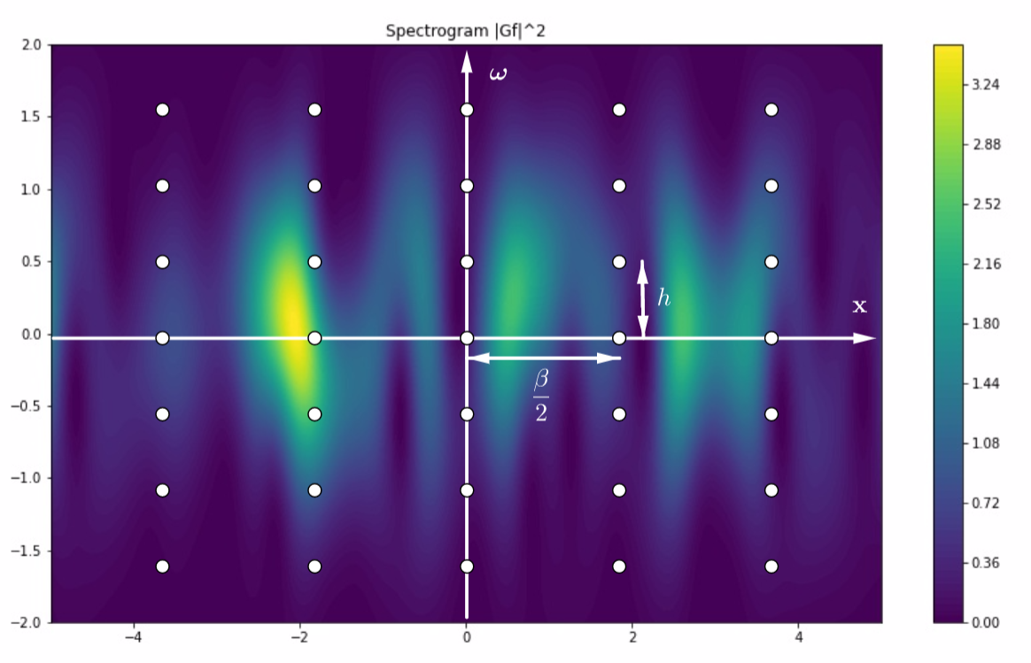
Refer to caption
Figure 4. The contour plot depicts the spectrogram of a function f∈Vβ∞​(φ)f\in V_{\beta}^{\infty}(\varphi) and the white dots visualize the location of the samples 𝔖\mathfrak{S}. The values 2β\frac{2}{\beta} and 1h\frac{1}{h} are the densities in time (xx) resp. frequency (ω\omega) direction.

4.1. The numerical approximation routine ℛ\mathcal{R}

We start by presenting our reconstruction approach in an abstract setting, leaving the ansatz open for extensions to other signal classes (see Section 4.4). Assume for the time-being that the function ff has only the property of being measurable and bounded. Let p1<⋯<pJp_{1}<\cdots<p_{J} and γ>0\gamma>0 such that ff satisfies condition (P). For simplicity we assume that −p1=pJ≕s-p_{1}=p_{J}\eqqcolon s and set I=[−s,s]I=[-s,s]. The aim is to recover ff on the interval II. Generalizations to other intervals are straightforward and can be achieved by a simple translation. Motivated by Proposition 3.1 and Theorem 3.6 we define constants cjc_{j} by

cj=h​∑n∑k𝔖⁡(n,k)​Tβ2​n​φ0~​(pj),c_{j}=h\sum_{n}\sum_{k}\mathfrak{S}(n,k)T_{\frac{\beta}{2}n}\widetilde{\varphi_{0}}(p_{j}),

local reconstructive functions LjL_{j} by

Lj​(ω)=hcj​∑n∑k𝔖⁡(n,k)​e2​π​i​ω​h​k​Tβ2​n​φω~​(pj+ω)L_{j}(\omega)=\frac{h}{\sqrt{c_{j}}}\sum_{n}\sum_{k}\mathfrak{S}(n,k)e^{2\pi i\omega hk}T_{\frac{\beta}{2}n}\widetilde{\varphi_{\omega}}(p_{j}+\omega)

and phases ν0,…,νJ−1∈𝕋\nu_{0},\dots,\nu_{J-1}\in{\mathbb{T}} by

ν0=1,νj=Lj​(pj+1−pj)|Lj​(pj+1−pj)|​(j=1,…,J−1).\nu_{0}=1,\ \ \nu_{j}=\frac{L_{j}(p_{j+1}-p_{j})}{|L_{j}(p_{j+1}-p_{j})|}\ (j=1,\dots,J-1).

Note that cj,Ljc_{j},L_{j} and νj\nu_{j} depend only on the sampling set 𝔖\mathfrak{S}. Assuming that LjL_{j} and νj\nu_{j} are well-defined, i.e. cj>0c_{j}>0 and Lj​(pj+1−pj)≠0L_{j}(p_{j+1}-p_{j})\neq 0, gives rise to the definition of a numerical approximation routine.

Definition 4.1.

Suppose that f:ℝ→ℂf:{\mathbb{R}}\to{\mathbb{C}} is a measurable and bounded map which satisfies condition (P) with γ>0\gamma>0 and p1<⋯<pJ∈ℝ,−p1=pJ=sp_{1}<\cdots<p_{J}\in{\mathbb{R}},-p_{1}=p_{J}=s. Let the grid XX be defined as in (30) and suppose that LjL_{j} and νj\nu_{j} are well-defined. The numerical approximation routine ℛ:[−s,s]→ℂ\mathcal{R}:[-s,s]\to{\mathbb{C}} of ff is defined as follows: if t∈[−s,s]t\in[-s,s] such that t∈(pj,pj+1]t\in(p_{j},p_{j+1}] with t=pj+ωt=p_{j}+\omega then

ℛ(t)=ν1⋯νj−1Lj(ω).\mathcal{R}(t)=\nu_{1}\cdots\nu_{j-1}L_{j}(\omega).

For t=p1=−st=p_{1}=-s we define ℛ​(t)=L1​(0)\mathcal{R}(t)=L_{1}(0).

In order to derive approximation results by means of the numerical approximation routine ℛ\mathcal{R}, we define for j=1,…,J−1j=1,\dots,J-1 the error term

(31) Ej​(ω)≔|fω​(pj+ω)−cj​Lj​(ω)¯|.E_{j}(\omega)\coloneqq|f_{\omega}(p_{j}+\omega)-\sqrt{c_{j}}\overline{L_{j}(\omega)}|.

This error term allows us to state conditions under which the functions LjL_{j} and the phases νj\nu_{j} are well-defined. More importantly, it yields an upper bound on the quotient distance of ff and ℛ\mathcal{R}.

Theorem 4.2.

Let f:ℝ→ℂf:{\mathbb{R}}\to{\mathbb{C}} be a measurable and bounded function which satisfies condition (P) with γ>0\gamma>0 and p1<⋯<pJ∈ℝ,−p1=pJ=sp_{1}<\cdots<p_{J}\in{\mathbb{R}},-p_{1}=p_{J}=s. If I=[−s,s]I=[-s,s], 0<ε≤min⁡{γ22​8,γ34​‖f‖L∞​(I)}0<\varepsilon\leq\min\left\{\frac{\gamma^{2}}{2\sqrt{8}},\frac{\gamma^{3}}{4\|f\|_{L^{\infty}(I)}}\right\} and

max1≤j≤J−1⁡‖Ej‖L∞​[0,pj+1−pj]≤ε\max_{1\leq j\leq J-1}\|E_{j}\|_{L^{\infty}[0,p_{j+1}-p_{j}]}\leq\varepsilon

then LjL_{j} and νj\nu_{j} are well-defined for every j∈{1,…,J}j\in\{1,\dots,J\}. Further, it holds that

minτ∈𝕋⁡‖f−τ​ℛ‖L∞​(I)≤32​(J−1)​max⁡{1,‖f‖L∞​(I)2}min⁡{γ,γ5}​(ε+ε2).\min_{\tau\in{\mathbb{T}}}\|f-\tau\mathcal{R}\|_{L^{\infty}(I)}\leq 32(J-1)\frac{\max\{1,\|f\|^{2}_{L^{\infty}(I)}\}}{\min\{\gamma,\gamma^{5}\}}(\varepsilon+\varepsilon^{2}).
Proof.

Let I≔[−s,s]I\coloneqq[-s,s] and Ij≔(pj,pj+1]I_{j}\coloneqq(p_{j},p_{j+1}] for j=1,…,J−1j=1,\dots,J-1.

Step 1: Upper bounding minτ∈𝕋⁡‖f−τ​ℛ‖L∞​(I)\min_{\tau\in{\mathbb{T}}}\|f-\tau\mathcal{R}\|_{L^{\infty}(I)}. Assume for the time-being that the phases νj\nu_{j} and the constants cjc_{j} are well-defined. Let t∈It\in I such that t∈(pj,pj+1]t\in(p_{j},p_{j+1}] with t=pj+ωt=p_{j}+\omega and 2≤j≤J−12\leq j\leq J-1. Then

(32) |f⁡(t)−f⁡(p1)|f⁡(p1)|​ℛ​(t)|≤|f(pj+ω)−f⁡(pj)|f⁡(pj)|Lj(ω)|+|f⁡(pj)|f⁡(pj)|Lj(ω)−f⁡(p1)|f⁡(p1)|ν1⋯νj−1Lj(ω)|=|f⁡(pj+ω)−f⁡(pj)|f⁡(pj)|​Lj​(ω)|+|f⁡(pj)|f⁡(pj)|−f⁡(p1)|f⁡(p1)|ν1⋯νj−1|⏟≔A​|Lj​(ω)|.\begin{split}&\left|f(t)-\frac{f(p_{1})}{|f(p_{1})|}\mathcal{R}(t)\right|\\ &\leq\left|f(p_{j}+\omega)-\frac{f(p_{j})}{|f(p_{j})|}L_{j}(\omega)\right|+\left|\frac{f(p_{j})}{|f(p_{j})|}L_{j}(\omega)-\frac{f(p_{1})}{|f(p_{1})|}\nu_{1}\cdots\nu_{j-1}L_{j}(\omega)\right|\\ &=\left|f(p_{j}+\omega)-\frac{f(p_{j})}{|f(p_{j})|}L_{j}(\omega)\right|+\underbrace{\left|\frac{f(p_{j})}{|f(p_{j})|}-\frac{f(p_{1})}{|f(p_{1})|}\nu_{1}\cdots\nu_{j-1}\right|}_{\coloneqq A}|L_{j}(\omega)|.\end{split}

The term AA can be bounded by

(33) A=|νj−1¯f⁡(pj)|f⁡(pj)|−f⁡(p1)|f⁡(p1)|ν1⋯νj−2|≤|νj−1¯f⁡(pj)|f⁡(pj)|−f⁡(pj−1)|f⁡(pj−1)||+|f⁡(pj−1)|f⁡(pj−1)|−f⁡(p1)|f⁡(p1)|ν1⋯νj−2|≤∑i=2j|f⁡(pi)|f⁡(pi)|−f⁡(pi−1)|f⁡(pi−1)|​νi−1|\begin{split}A&=\left|\overline{\nu_{j-1}}\frac{f(p_{j})}{|f(p_{j})|}-\frac{f(p_{1})}{|f(p_{1})|}\nu_{1}\cdots\nu_{j-2}\right|\\ &\leq\left|\overline{\nu_{j-1}}\frac{f(p_{j})}{|f(p_{j})|}-\frac{f(p_{j-1})}{|f(p_{j-1})|}\right|+\left|\frac{f(p_{j-1})}{|f(p_{j-1})|}-\frac{f(p_{1})}{|f(p_{1})|}\nu_{1}\cdots\nu_{j-2}\right|\\ &\leq\sum_{i=2}^{j}\left|\frac{f(p_{i})}{|f(p_{i})|}-\frac{f(p_{i-1})}{|f(p_{i-1})|}\nu_{i-1}\right|\end{split}

where the third inequality follows by induction. Each summand in the last term of the sum above satisfies

(34) |f⁡(pi)|f⁡(pi)|−f⁡(pi−1)|f⁡(pi−1)|​νi−1|=|1|f⁡(pi)|​f​(pi)−1|Li−1​(pi−pi−1)|​f⁡(pi−1)|f⁡(pi−1)|​Li−1​(pi−pi−1)|≤|f⁡(pi)|​|1|f⁡(pi)|−1|Li−1​(pi−pi−1)||+1|Li−1​(pi−pi−1)|​|f⁡(pi)−f⁡(pi−1)|f⁡(pi−1)|​Li−1​(pi−pi−1)|=|f⁡(pi)|​||f⁡(pi)|−|f⁡(pi−1)|f⁡(pi−1)|​Li−1​(pi−pi−1)||f⁡(pi)|​|Li−1​(pi−pi−1)||+1|Li−1​(pi−pi−1)|​|f⁡(pi)−f⁡(pi−1)|f⁡(pi−1)|​Li−1​(pi−pi−1)|≤2|Li−1​(pi−pi−1)|​|f⁡(pi)−f⁡(pi−1)|f⁡(pi−1)|​Li−1​(pi−pi−1)|.\begin{split}&\left|\frac{f(p_{i})}{|f(p_{i})|}-\frac{f(p_{i-1})}{|f(p_{i-1})|}\nu_{i-1}\right|\\ &=\left|\frac{1}{|f(p_{i})|}f(p_{i})-\frac{1}{|L_{i-1}(p_{i}-p_{i-1})|}\frac{f(p_{i-1})}{|f(p_{i-1})|}L_{i-1}(p_{i}-p_{i-1})\right|\\ &\leq|f(p_{i})|\left|\frac{1}{|f(p_{i})|}-\frac{1}{|L_{i-1}(p_{i}-p_{i-1})|}\right|\\ &+\frac{1}{|L_{i-1}(p_{i}-p_{i-1})|}\left|f(p_{i})-\frac{f(p_{i-1})}{|f(p_{i-1})|}L_{i-1}(p_{i}-p_{i-1})\right|\\ &=|f(p_{i})|\left|\frac{|f(p_{i})|-|\frac{f(p_{i-1})}{|f(p_{i-1})|}L_{i-1}(p_{i}-p_{i-1})|}{|f(p_{i})||L_{i-1}(p_{i}-p_{i-1})|}\right|\\ &+\frac{1}{|L_{i-1}(p_{i}-p_{i-1})|}\left|f(p_{i})-\frac{f(p_{i-1})}{|f(p_{i-1})|}L_{i-1}(p_{i}-p_{i-1})\right|\\ &\leq\frac{2}{|L_{i-1}(p_{i}-p_{i-1})|}\left|f(p_{i})-\frac{f(p_{i-1})}{|f(p_{i-1})|}L_{i-1}(p_{i}-p_{i-1})\right|.\end{split}

Combining the inequalties (32), (33) and (34) gives

|f⁡(t)−f⁡(p1)|f⁡(p1)|​ℛ​(t)|≤|f⁡(pj+ω)−f⁡(pj)|f⁡(pj)|​Lj​(ω)|+2|Lj​(ω)|∑i=2j1|Li−1​(pi−pi−1)|​|f⁡(pi)−f⁡(pi−1)|f⁡(pi−1)|​Li−1​(pi−pi−1)|.\begin{split}&\left|f(t)-\frac{f(p_{1})}{|f(p_{1})|}\mathcal{R}(t)\right|\leq\left|f(p_{j}+\omega)-\frac{f(p_{j})}{|f(p_{j})|}L_{j}(\omega)\right|\\ &+2|L_{j}(\omega)|\sum_{i=2}^{j}\frac{1}{|L_{i-1}(p_{i}-p_{i-1})|}\left|f(p_{i})-\frac{f(p_{i-1})}{|f(p_{i-1})|}L_{i-1}(p_{i}-p_{i-1})\right|.\end{split}

Observe that pi∈Ii−1p_{i}\in I_{i-1} and f⁡(pi)=f⁡(pi−1+(pi−pi−1))f(p_{i})=f(p_{i-1}+(p_{i}-p_{i-1})). Therefore, if we set

Q≔max1≤j≤J−1∥f(pj+⋅)−f⁡(pj)|f⁡(pj)|Lj∥L∞​(Ij)Q\coloneqq\max_{1\leq j\leq J-1}\|f(p_{j}+\cdot)-\tfrac{f(p_{j})}{|f(p_{j})|}L_{j}\|_{L^{\infty}(I_{j})}

then

|f⁡(t)−f⁡(p1)|f⁡(p1)|​ℛ​(t)|≤Q+2​Q​|Lj​(ω)|​∑i=2j1|Li−1​(pi−pi−1)|.\left|f(t)-\frac{f(p_{1})}{|f(p_{1})|}\mathcal{R}(t)\right|\leq Q+2Q|L_{j}(\omega)|\sum_{i=2}^{j}\frac{1}{|L_{i-1}(p_{i}-p_{i-1})|}.

Observing that

|Lj​(ω)|≤|f⁡(pj+ω)−f⁡(pj)|f⁡(pj)|​Lj​(ω)|+|f⁡(pj+ω)|≤Q+‖f‖L∞​(I),|L_{j}(\omega)|\leq\left|f(p_{j}+\omega)-\frac{f(p_{j})}{|f(p_{j})|}L_{j}(\omega)\right|+|f(p_{j}+\omega)|\leq Q+\|f\|_{L^{\infty}(I)},

gives

(35) minτ∈𝕋⁡‖f−τ​ℛ‖L∞​(I)≤Q+2​Q​(‖f‖L∞​(I)+Q)​∑i=2j1|Li−1​(pi−pi−1)|.\min_{\tau\in{\mathbb{T}}}\|f-\tau\mathcal{R}\|_{L^{\infty}(I)}\leq Q+2Q\left(\|f\|_{L^{\infty}(I)}+Q\right)\sum_{i=2}^{j}\frac{1}{|L_{i-1}(p_{i}-p_{i-1})|}.

Step 2. Well-definedness of cjc_{j}. If the map SjS_{j} is defined by

Sj​(ω)=cj​Lj​(ω)¯=h​∑n∑k𝔖⁡(n,k)​e−2​π​i​ω​h​k​Tβ2​n​φω~​(pj+ω),S_{j}(\omega)=\sqrt{c_{j}}\overline{L_{j}(\omega)}=h\sum_{n}\sum_{k}\mathfrak{S}(n,k)e^{-2\pi i\omega hk}T_{\frac{\beta}{2}n}\widetilde{\varphi_{\omega}}(p_{j}+\omega),

then Ej​(ω)=|fω​(pj+ω)−Sj​(ω)|.E_{j}(\omega)=|f_{\omega}(p_{j}+\omega)-S_{j}(\omega)|. Observe that cj=Sj​(0),f0​(pj)=|f⁡(pj)|2c_{j}=S_{j}(0),f_{0}(p_{j})=|f(p_{j})|^{2} and

cj≥|f⁡(pj)|2−||f⁡(pj)|2−cj|≥γ2−|f0​(pj)−Sj​(0)|=γ2−Ej​(0).c_{j}\geq|f(p_{j})|^{2}-||f(p_{j})|^{2}-c_{j}|\geq\gamma^{2}-|f_{0}(p_{j})-S_{j}(0)|=\gamma^{2}-E_{j}(0).

By assumption we have Ej​(0)≤max1≤j≤J−1⁡‖Ej‖L∞​[0,pj+1−pj]≤ε≤γ22E_{j}(0)\leq\max_{1\leq j\leq J-1}\|E_{j}\|_{L^{\infty}[0,p_{j+1}-p_{j}]}\leq\varepsilon\leq\frac{\gamma^{2}}{2} which gives

(36) cj≥γ22.c_{j}\geq\frac{\gamma^{2}}{2}.

In particular, the constants cjc_{j} are well-defined.

Step 3: Upper bounding Ej​(ω)E_{j}(\omega). We have shown that the constants cjc_{j} are well-defined. Recalling that if f⁡(pj)≠0f(p_{j})\neq 0 then the identity 1f⁡(pj)¯​fω​(pj+ω)¯\frac{1}{\overline{f(p_{j})}}\overline{f_{\omega}(p_{j}+\omega)} holds for every ω∈ℝ\omega\in{\mathbb{R}}. We can continue with the following estimate:

(37) |f⁡(pj+ω)−f⁡(pj)|f⁡(pj)|​Lj​(ω)|=|1f⁡(pj)¯​fω​(pj+ω)¯−f⁡(pj)|f⁡(pj)|​1cj​Sj​(ω)¯|=|1f⁡(pj)​fω​(pj+ω)−|f⁡(pj)|f⁡(pj)​1cj​Sj​(ω)|≤1cj​|fω​(pj+ω)−Sj​(ω)|+|f⁡(pj)|f⁡(pj)|​(1f⁡(pj)−|f⁡(pj)|f⁡(pj)​1cj)|​|fω​(pj+ω)|=1cj​|fω​(pj+ω)−Sj​(ω)|+|1|f⁡(pj)|−1cj|​|fω​(pj+ω)|=1cj​|fω​(pj+ω)−Sj​(ω)|+|cj−|f⁡(pj)|2|cj​(cj+|f​(pj)|)​|f⁡(pj+ω)|≤1cj​|fω​(pj+ω)−Sj​(ω)|+‖f‖L∞​(I)cj​(cj+|f​(pj)|)​|f0​(pj)−Sj​(0)|=1cj​Ej​(ω)+‖f‖L∞​(I)cj​(cj+|f​(pj)|)​Ej​(0).\begin{split}&|f(p_{j}+\omega)-\tfrac{f(p_{j})}{|f(p_{j})|}L_{j}(\omega)|=\left|\frac{1}{\overline{f(p_{j})}}\overline{f_{\omega}(p_{j}+\omega)}-\frac{f(p_{j})}{|f(p_{j})|}\frac{1}{\sqrt{c_{j}}}\overline{S_{j}(\omega)}\right|\\ &=\left|\frac{1}{f(p_{j})}f_{\omega}(p_{j}+\omega)-\frac{|f(p_{j})|}{f(p_{j})}\frac{1}{\sqrt{c_{j}}}S_{j}(\omega)\right|\\ &\leq\frac{1}{\sqrt{c_{j}}}|f_{\omega}(p_{j}+\omega)-S_{j}(\omega)|+\left|\frac{f(p_{j})}{|f(p_{j})|}\left(\frac{1}{f(p_{j})}-\frac{|f(p_{j})|}{f(p_{j})}\frac{1}{\sqrt{c_{j}}}\right)\right||f_{\omega}(p_{j}+\omega)|\\ &=\frac{1}{\sqrt{c_{j}}}|f_{\omega}(p_{j}+\omega)-S_{j}(\omega)|+\left|\frac{1}{|f(p_{j})|}-\frac{1}{\sqrt{c_{j}}}\right||f_{\omega}(p_{j}+\omega)|\\ &=\frac{1}{\sqrt{c_{j}}}|f_{\omega}(p_{j}+\omega)-S_{j}(\omega)|+\frac{|c_{j}-|f(p_{j})|^{2}|}{\sqrt{c_{j}}(\sqrt{c_{j}}+|f(p_{j})|)}|f(p_{j}+\omega)|\\ &\leq\frac{1}{\sqrt{c_{j}}}|f_{\omega}(p_{j}+\omega)-S_{j}(\omega)|+\frac{\|f\|_{L^{\infty}(I)}}{\sqrt{c_{j}}(\sqrt{c_{j}}+|f(p_{j})|)}|f_{0}(p_{j})-S_{j}(0)|\\ &=\frac{1}{\sqrt{c_{j}}}E_{j}(\omega)+\frac{\|f\|_{L^{\infty}(I)}}{\sqrt{c_{j}}(\sqrt{c_{j}}+|f(p_{j})|)}E_{j}(0).\end{split}

Using the bound obtained in equation (36) together with the fact that |f⁡(pj)|≥γ|f(p_{j})|\geq\gamma yields

(38) |f⁡(pj+ω)−f⁡(pj)|f⁡(pj)|​Lj​(ω)|≤2γ​Ej​(ω)+‖f‖L∞​(I)γ2​Ej​(0).|f(p_{j}+\omega)-\tfrac{f(p_{j})}{|f(p_{j})|}L_{j}(\omega)|\leq\frac{\sqrt{2}}{\gamma}E_{j}(\omega)+\frac{\|f\|_{L^{\infty}(I)}}{\gamma^{2}}E_{j}(0).

Step 4: Well-definedness of the phases νj\nu_{j}. We use the upper bound on EjE_{j} to show that the phases νj\nu_{j} are well-defined. First, observe that

|Lj​(pj+1−pj)|≥|f⁡(pj+1)|−|f⁡(pj+1)−f⁡(pj)|f⁡(pj)|​Lj​(pj+1−pj)|.|L_{j}(p_{j+1}-p_{j})|\geq|f(p_{j+1})|-|f(p_{j+1})-\tfrac{f(p_{j})}{|f(p_{j})|}L_{j}(p_{j+1}-p_{j})|.

Since Ej​(ω)≤max1≤j≤J−1⁡‖Ej‖L∞​[0,pj+1−pj]≤εE_{j}(\omega)\leq\max_{1\leq j\leq J-1}\|E_{j}\|_{L^{\infty}[0,p_{j+1}-p_{j}]}\leq\varepsilon for every ω∈[0,pj+1−pj]\omega\in[0,p_{j+1}-p_{j}] and since ε\varepsilon satisfies the upper bound ε≤min⁡{γ22​8,γ34​‖f‖L∞​(I)}\varepsilon\leq\min\left\{\frac{\gamma^{2}}{2\sqrt{8}},\frac{\gamma^{3}}{4\|f\|_{L^{\infty}(I)}}\right\} it follows it follows from the upper bound obtained in (37) that |f⁡(pj+1)−f⁡(pj)|f⁡(pj)|​Lj​(pj+1−pj)|≤γ2.|f(p_{j+1})-\tfrac{f(p_{j})}{|f(p_{j})|}L_{j}(p_{j+1}-p_{j})|\leq\frac{\gamma}{2}. In particular, this shows that

(39) |Lj​(pj+1−pj)|≥γ2.|L_{j}(p_{j+1}-p_{j})|\geq\frac{\gamma}{2}.

Thus, the phases νj\nu_{j} are well-defined for all jj.

Step 5: Combining step 1-4.

If QQ is given as above then from inequality (38) we obtain

Q≤2​max⁡{1,‖f‖L∞​(I)}min⁡{γ,γ2}​maxj=1,…,J⁡‖Ej‖L∞+Ej​(0)⏟≔ΞQ\leq\frac{\sqrt{2}\max\{1,\|f\|_{L^{\infty}(I)}\}}{\min\{\gamma,\gamma^{2}\}}\underbrace{\max_{j=1,\dots,J}\|E_{j}\|_{L^{\infty}}+E_{j}(0)}_{\coloneqq\Xi}

Inequality (35) and the lower bound 39 implies that

minτ∈𝕋⁡‖f−τ​ℛ‖L∞​(I)≤2​max⁡{1,‖f‖L∞​(I)}min⁡{γ,γ2}​Ξ+4​2​(J−1)​max⁡{‖f‖L∞​(I),‖f‖L∞​(I)2}γ​min⁡{γ,γ2}​Ξ+8​(J−1)​max⁡{1,‖f‖L∞​(I)2}γ​min⁡{γ2,γ4}​Ξ2≤8​(J−1)​max⁡{1,‖f‖L∞​(I),‖f‖L∞​(I)2}min⁡{γ,γ2,γ4,γ5}​(2​Ξ+Ξ2)\begin{split}&\min_{\tau\in{\mathbb{T}}}\|f-\tau\mathcal{R}\|_{L^{\infty}(I)}\leq\frac{\sqrt{2}\max\{1,\|f\|_{L^{\infty}(I)}\}}{\min\{\gamma,\gamma^{2}\}}\Xi\\ &+\frac{4\sqrt{2}(J-1)\max\{\|f\|_{L^{\infty}(I)},\|f\|_{L^{\infty}(I)}^{2}\}}{\gamma\min\{\gamma,\gamma^{2}\}}\Xi+\frac{8(J-1)\max\{1,\|f\|_{L^{\infty}(I)}^{2}\}}{\gamma\min\{\gamma^{2},\gamma^{4}\}}\Xi^{2}\\ &\leq 8(J-1)\frac{\max\{1,\|f\|_{L^{\infty}(I)},\|f\|_{L^{\infty}(I)}^{2}\}}{\min\{\gamma,\gamma^{2},\gamma^{4},\gamma^{5}\}}(2\Xi+\Xi^{2})\end{split}

In particular, the assumption on ε\varepsilon and the fact that min⁡{γ,γ2,γ4,γ5}=min⁡{γ,γ5}\min\{\gamma,\gamma^{2},\gamma^{4},\gamma^{5}\}=\min\{\gamma,\gamma^{5}\} and max⁡{1,‖f‖L∞​(I),‖f‖L∞​(I)2}=max⁡{1,‖f‖L∞​(I)2}\max\{1,\|f\|_{L^{\infty}(I)},\|f\|_{L^{\infty}(I)}^{2}\}=\max\{1,\|f\|_{L^{\infty}(I)}^{2}\} gives

minτ∈𝕋⁡‖f−τ​ℛ‖L∞​(I)≤32​(J−1)​max⁡{1,‖f‖L∞​(I)2}min⁡{γ1,γ5}​(ε+ε2).\min_{\tau\in{\mathbb{T}}}\|f-\tau\mathcal{R}\|_{L^{\infty}(I)}\leq 32(J-1)\frac{\max\{1,\|f\|_{L^{\infty}(I)}^{2}\}}{\min\{\gamma^{1},\gamma^{5}\}}(\varepsilon+\varepsilon^{2}).

∎

4.2. Application to Gaussian shift-invariant spaces

Recall that the inner products ⟨fω,Tx​φω⟩\langle f_{\omega},T_{x}\varphi_{\omega}\rangle were given in terms of the Fourier integral

(40) ⟨fω,Tx​φω⟩=∫ℝ|𝒢​f​(x,t)|2​e−2​π​i​ω​t​𝑑t.\langle f_{\omega},T_{x}\varphi_{\omega}\rangle=\int_{\mathbb{R}}|\mathcal{G}f(x,t)|^{2}e^{-2\pi i\omega t}\,dt.

To allow an approximation of functions in f∈Vβ∞​(φ)f\in V_{\beta}^{\infty}(\varphi) from |𝒢​f​(X)||\mathcal{G}f(X)| where XX is a set of finitely many sampling points, we discretize the above integral using a suitable quadrature formula. If σ\sigma is the standard deviation of the Gaussian φ\varphi then we define σ′≔12​π​σ\sigma^{\prime}\coloneqq\frac{1}{2\pi\sigma}. The choice of a quadrature formula is based on the following factorization formula of the spectrogram.

Theorem 4.3.

If f∈Vβ∞​(φ)f\in V_{\beta}^{\infty}(\varphi) has defining sequence c∈ℓ∞​(ℤ)c\in\ell^{\infty}({\mathbb{Z}}) then the spectrogram of ff factors as

(41) |𝒢​f​(x,t)|2=π​σ2​φσ′​(t)​Sx​(t)|\mathcal{G}f(x,t)|^{2}=\pi\sigma^{2}\varphi^{\sigma^{\prime}}(t)S_{x}(t)

where Sx​(t)=∑ℓbℓ​(x)​eπ​i​β​ℓ​tS_{x}(t)=\sum_{\ell}b_{\ell}(x)e^{\pi i\beta\ell t} is a trigonometric series whose coefficients satisfy the Gaussian bound

|bℓ​(x)|≤‖c‖∞2​(1+σβ​2​π)​e−18​(β​ℓσ)2.|b_{\ell}(x)|\leq\|c\|_{\infty}^{2}\left(1+\frac{\sigma}{\beta}\sqrt{2\pi}\right)e^{-\frac{1}{8}(\frac{\beta\ell}{\sigma})^{2}}.

In particular, for every x∈ℝx\in{\mathbb{R}} the map z↦|𝒢​f​(x,z)|2z\mapsto|\mathcal{G}f(x,z)|^{2} extends from ℝ{\mathbb{R}} to an entire function on ℂ{\mathbb{C}}. The extension is given by the map ℂ∋z↦π​σ2​φσ′​(z)​Sx​(z){\mathbb{C}}\ni z\mapsto\pi\sigma^{2}\varphi^{\sigma^{\prime}}(z)S_{x}(z).

Proof.

See the Appendix 5.4. ∎

Recall that for h>0h>0 and H∈ℕ∪{∞}H\in{\mathbb{N}}\cup\{\infty\} the trapezoidal rule approximation of a map W:ℝ→ℂW:{\mathbb{R}}\to{\mathbb{C}} is defined by

(42) IhH​(W)≔h​∑k=−HHW⁡(h​k).I_{h}^{H}(W)\coloneqq h\sum_{k=-H}^{H}W(hk).

Applying this quadrature rule to the Fourier integral (40) gives

(43) IhH​(t↦|𝒢​f​(x,t)|2​e−2​π​i​ω​t)=h​∑k=−HH|𝒢​f​(x,h​k)|2​e−2​π​i​ω​h​k,I_{h}^{H}(t\mapsto|\mathcal{G}f(x,t)|^{2}e^{-2\pi i\omega t})=h\sum_{k=-H}^{H}|\mathcal{G}f(x,hk)|^{2}e^{-2\pi i\omega hk},

which essentially represents the discrete Fourier transform. We apply a classical result on the exponentially convergent trapezoidal rule [34, Theorem 5.1].

Theorem 4.4 (Trefethen-Weideman).

Let a>0a>0 and suppose that WW is an analytic map in the strip Ua={z∈ℂ:|Im⁡(z)|<a}U_{a}=\{z\in{\mathbb{C}}:|\mathrm{Im}(z)|<a\}. Suppose further that W⁡(x)→0W(x)\to 0 uniformly as |x|→∞|x|\to\infty in the strip. If

M⁡(W)≔supt+i​y∈Ua∫−∞∞|W⁡(t+i​y)|​𝑑t<∞M(W)\coloneqq\sup_{t+iy\in U_{a}}\int_{-\infty}^{\infty}|W(t+iy)|\,dt<\infty

then, for any h>0h>0, the trapezoidal rule approximation Ih∞​(W)I_{h}^{\infty}(W) of ∫ℝW\int_{\mathbb{R}}W exists and satisfies

|Ih∞​(W)−∫ℝW|≤2​M​(W)e2​π​a/h−1.\left|I_{h}^{\infty}(W)-\int_{\mathbb{R}}W\right|\leq\frac{2M(W)}{e^{2\pi a/h}-1}.

The quantity 2​M2M in the numerator is optimal.

Truncating the series which corresponds to the biorthogonal expansion of fωf_{\omega} and using the approximation (43) of the inner products given in (40), results in the map

(44) S⁡(ω)=h​∑n=−NN∑k=−HH𝔖⁡(n,k)​e−2​π​i​ω​h​k​Tβ2​n​φω~​(p+ω),N∈ℕ,S(\omega)=h\sum_{n=-N}^{N}\sum_{k=-H}^{H}\mathfrak{S}(n,k)e^{-2\pi i\omega hk}T_{\frac{\beta}{2}n}\widetilde{\varphi_{\omega}}(p+\omega),\ \ N\in{\mathbb{N}},

which is precisely the function cj​Lj¯\sqrt{c_{j}}\overline{L_{j}} (with p=pjp=p_{j}) appearing in the error term EjE_{j} defined in equation (31). The pointwise distance between the map ω↦fω​(p+ω)\omega\mapsto f_{\omega}(p+\omega) and SS can be upper bounded as follows.

Lemma 4.5.

Assume that f∈Vβ∞​(φ)f\in V_{\beta}^{\infty}(\varphi) has defining sequence c∈ℓ∞​(ℤ)c\in\ell^{\infty}({\mathbb{Z}}). Suppose that N=⌈2β​(s+r2)⌉+mN=\lceil\frac{2}{\beta}(s+\frac{r}{2})\rceil+m for some m∈ℕm\in{\mathbb{N}} and some r,s>0r,s>0. Let h>0h>0 and H∈ℕH\in{\mathbb{N}}. Then for every p∈[−s,s]p\in[-s,s] and every ω∈[0,r]\omega\in[0,r] we have the error bound

(45) |fω​(p+ω)−S⁡(ω)|≤4​π​K​eω24​σ2​σν​β​(1+σβ​2​2​π)2​‖c‖∞2​e−ν​β2​m+2​π​K​eω24​σ2+|ω|σ+1​σ​(2+4ν​β)​(1+σβ​2​2​π)2​‖c‖∞2​1e1σ​h−1+π​K​eω24​σ2​σ​(2+4ν​β)​(1+σβ​2​2​π)2​‖c‖∞2​e−2​(π​H​h​σ)2+2​K​eω24​σ2​(2+4ν​β)​h​‖η‖∞\begin{split}&|f_{\omega}(p+\omega)-S(\omega)|\\ &\leq 4\sqrt{\pi}Ke^{\frac{\omega^{2}}{4\sigma^{2}}}\frac{\sigma}{\nu\beta}\left(1+\frac{\sigma}{\beta}2\sqrt{2\pi}\right)^{2}\|c\|_{\infty}^{2}e^{-\frac{\nu\beta}{2}m}\\ &+2\sqrt{\pi}Ke^{\frac{\omega^{2}}{4\sigma^{2}}+\frac{|\omega|}{\sigma}+1}\sigma\left(2+\frac{4}{\nu\beta}\right)\left(1+\frac{\sigma}{\beta}2\sqrt{2\pi}\right)^{2}\|c\|_{\infty}^{2}\frac{1}{e^{\frac{1}{\sigma h}}-1}\\ &+\sqrt{\pi}Ke^{\frac{\omega^{2}}{4\sigma^{2}}}\sigma\left(2+\frac{4}{\nu\beta}\right)\left(1+\frac{\sigma}{\beta}2\sqrt{2\pi}\right)^{2}\|c\|_{\infty}^{2}e^{-2(\pi Hh\sigma)^{2}}\\ &+\sqrt{2}Ke^{\frac{\omega^{2}}{4\sigma^{2}}}\left(2+\frac{4}{\nu\beta}\right)h\|\eta\|_{\infty}\end{split}

where K=K⁡(σ,β)K=K(\sigma,\beta) and ν=ν⁡(σ,β)\nu=\nu(\sigma,\beta) denote the decay constants of the dual generator as defined in (29).

Proof.

See the Appendix 5.5. ∎

Lemma 4.5 becomes meaningful if we interpret it in a qualitative way: recall that the constants KK and ν\nu depend only on σ\sigma and β\beta. Suppose that ff satisfies condition (P) and that the variance σ2\sigma^{2} and the step-size β\beta are fixed, i.e. both the window function and the underlying signal space is fixed. Under these assumption, it follows from inequality (45) and the definition of the error terms EjE_{j} that

(46) max1≤j≤J−1∥Ej∥L∞​[0,pj+1−pj]≲σ,β,r∥c∥∞2e−a​m+∥c∥∞21e1σ​h−1+∥c∥∞2e−b​(H​h)2+h∥η∥∞\max_{1\leq j\leq J-1}\|E_{j}\|_{L^{\infty}[0,p_{j+1}-p_{j}]}\lesssim_{\sigma,\beta,r}\|c\|_{\infty}^{2}e^{-am}+\|c\|_{\infty}^{2}\frac{1}{e^{\frac{1}{\sigma h}}-1}+\|c\|_{\infty}^{2}e^{-b(Hh)^{2}}+h\|\eta\|_{\infty}

where aa and bb are constants depending only on σ\sigma and β\beta. The constant rr is given by

(47) r≔max1≤j≤J−1⁡(pj+1−pj).r\coloneqq\max_{1\leq j\leq J-1}(p_{j+1}-p_{j}).

Let the universal constant in inequality (46) be denoted by 𝒟=𝒟⁡(σ,β,r)\mathcal{D}=\mathcal{D}(\sigma,\beta,r). Then the following approximation result holds.

Theorem 4.6.

Assume that f∈Vβ∞​(φ)f\in V_{\beta}^{\infty}(\varphi) has defining sequence c∈ℓ∞​(ℤ)c\in\ell^{\infty}({\mathbb{Z}}) and satisfies condition (P) with p1<⋯<pJ∈ℝ,−p1=pJ=sp_{1}<\cdots<p_{J}\in{\mathbb{R}},-p_{1}=p_{J}=s and γ>0\gamma>0. Let r≔max1≤j≤J−1⁡(pj+1−pj)r\coloneqq\max_{1\leq j\leq J-1}(p_{j+1}-p_{j}) and let ε\varepsilon be chosen as in Theorem 4.2, i.e. 0<ε≤min⁡{γ22​8,γ34​‖f‖L∞​(I)}.0<\varepsilon\leq\min\left\{\frac{\gamma^{2}}{2\sqrt{8}},\frac{\gamma^{3}}{4\|f\|_{L^{\infty}(I)}}\right\}. Suppose that the sampling density 1h\frac{1}{h} in frequency direction satisfies

1h≥σ​log⁡(4​𝒟​‖c‖∞2​(J−1)ε+1)\frac{1}{h}\geq\sigma\log\left(\frac{4\mathcal{D}\|c\|_{\infty}^{2}(J-1)}{\varepsilon}+1\right)

and the measurements are given on the grid

X=β2​{−N,…,N}×h⁡{−H,…,H}X=\tfrac{\beta}{2}\{-N,\dots,N\}\times h\{-H,\dots,H\}

such that the grid size characterizing parameters N,HN,H satisfy

H≥1h​(1b​log⁡(4​𝒟​‖c‖∞2​(J−1)ε))12H\geq\frac{1}{h}\left(\frac{1}{b}\log\left(\frac{4\mathcal{D}\|c\|_{\infty}^{2}(J-1)}{\varepsilon}\right)\right)^{\frac{1}{2}}

and

N≥⌈2β​(s+r2)⌉+1a​log⁡(4​𝒟​‖c‖∞2​(J−1)ε).N\geq\lceil\tfrac{2}{\beta}(s+\tfrac{r}{2})\rceil+\frac{1}{a}\log\left(\frac{4\mathcal{D}\|c\|_{\infty}^{2}(J-1)}{\varepsilon}\right).

Then the following holds: if the noise level does not exceed ε4​h​(J−1)​𝒟\frac{\varepsilon}{4h(J-1)\mathcal{D}}, i.e. ‖η‖∞≤ε4​h​(J−1)​𝒟\|\eta\|_{\infty}\leq\frac{\varepsilon}{4h(J-1)\mathcal{D}}, then

(48) minτ∈𝕋⁡‖f−τ​ℛ‖L∞​[−s,s]≤32​max⁡{1,‖f‖L∞​(I)2}min⁡{γ,γ5}​(ε+ε2)\min_{\tau\in{\mathbb{T}}}\|f-\tau\mathcal{R}\|_{L^{\infty}[-s,s]}\leq 32\frac{\max\{1,\|f\|^{2}_{L^{\infty}(I)}\}}{\min\{\gamma,\gamma^{5}\}}(\varepsilon+\varepsilon^{2})

where ℛ\mathcal{R} denotes the numerical approximation routine.

Proof.

Denote the four summands on the right-hand side of inequality (46) by Ξ1,…,Ξ4\Xi_{1},\dots,\Xi_{4}. It follows that if 𝒟​Ξi≤ε4​(J−1)\mathcal{D}\Xi_{i}\leq\frac{\varepsilon}{4(J-1)} for i=1,…,4i=1,\dots,4 then

maxj=1,…,J−1⁡‖Ej‖L∞​[0,pj+1−pj]≤εJ−1.\max_{j=1,\dots,J-1}\|E_{j}\|_{L^{\infty}[0,p_{j+1}-p_{j}]}\leq\frac{\varepsilon}{J-1}.

Elementary manipulations show that the condition 𝒟​Ξi≤ε4​(J−1)\mathcal{D}\Xi_{i}\leq\frac{\varepsilon}{4(J-1)} for i=1,…,4i=1,\dots,4 is satisfied by the above assumptions on h,H,Nh,H,N and ‖η‖∞\|\eta\|_{\infty}. The statement is therefore a consequence of Theorem 4.2. ∎

Based on the previous statement we can study the growth of the number of samples needed to achieve the bound (48) for an increasing length of the reconstruction interval I=[−s,s]I=[-s,s]. Consider the noiseless case, η=0\eta=0. Suppose that condition (P) holds on the entire real-line, i.e. there exists a partition

P=⋯<p−1<p0<p1<⋯,|f⁡(pj)|≥γP=\cdots<p_{-1}<p_{0}<p_{1}<\cdots,\ |f(p_{j})|\geq\gamma

so that the maximal distance between two consecutive points pjp_{j} and pj+1p_{j+1} remains upper bounded by rr, i.e. supj∈ℤ(pj+1−pj)≤r.\sup_{j\in{\mathbb{Z}}}(p_{j+1}-p_{j})\leq r. By going to a sub-partition we can always assume that for an interval [−s,s][-s,s] there exists pj,pk∈Pp_{j},p_{k}\in P with pj≤−s,pk≥sp_{j}\leq-s,p_{k}\geq s and k−j≤4​sr+𝒪⁡(1)k-j\leq\frac{4s}{r}+\mathcal{O}(1). Therefore, the assumptions on the bounds on h,Hh,H and NN as stated in Theorem 4.6 can be re-written as

1h≥σ​log⁡(𝒟′​‖c‖∞2​sε+1),H≥1h​(1b​log⁡(𝒟′​‖c‖∞2​sε))12,\frac{1}{h}\geq\sigma\log\left(\frac{\mathcal{D}^{\prime}\|c\|_{\infty}^{2}s}{\varepsilon}+1\right),H\geq\frac{1}{h}\left(\frac{1}{b}\log\left(\frac{\mathcal{D}^{\prime}\|c\|_{\infty}^{2}s}{\varepsilon}\right)\right)^{\frac{1}{2}},
N≥⌈2β​(s+r2)⌉+1a​log⁡(𝒟′​‖c‖∞2​sε).N\geq\lceil\tfrac{2}{\beta}(s+\tfrac{r}{2})\rceil+\frac{1}{a}\log\left(\frac{\mathcal{D}^{\prime}\|c\|_{\infty}^{2}s}{\varepsilon}\right).

where 𝒟′\mathcal{D}^{\prime} is a constant depending only on σ,β\sigma,\beta and rr. A direct consequence is

Corollary 4.7.

Under the assumptions above, the following holds: in order to achieve a reconstruction of f∈Vβ∞​(φ)f\in V_{\beta}^{\infty}(\varphi) with defining sequence c∈ℓ∞​(ℤ)c\in\ell^{\infty}({\mathbb{Z}}) on an interval I=[−s,s]I=[-s,s] of length 2​s2s up an error bound of the form (48) using the numerical approximation routine ℛ\mathcal{R}, the number 𝒩⁡(s)\mathcal{N}(s) of spectrogram samples satisfies the upper growth estimate

𝒩(s)≲σ,β,rlog(s​‖c‖∞2ε)32(s+log(s​‖c‖∞2ε)).\mathcal{N}(s)\lesssim_{\sigma,\beta,r}\log\left(\frac{s\|c\|_{\infty}^{2}}{\varepsilon}\right)^{\frac{3}{2}}\left(s+\log\left(\frac{s\|c\|_{\infty}^{2}}{\varepsilon}\right)\right).

Assumptions on σ\sigma and β\beta turn the qualitative results above into quantitative results by means of explicit upper bounds on a,ba,b and 𝒟\mathcal{D}. This can be done in a similar fashion as at the end of Section 3 and exploiting Lemma 3.11.

Proposition 4.8.

If β4≤σ≤β2≤1\frac{\beta}{4}\leq\sigma\leq\frac{\beta}{2}\leq 1 and r≤2​σr\leq 2\sigma then

𝒟≤40000​(2+16β)​(1+σβ​2​2​π)2,a≥β8,b≥2​π2​σ2.\mathcal{D}\leq 40000\left(2+\frac{16}{\beta}\right)\left(1+\frac{\sigma}{\beta}2\sqrt{2\pi}\right)^{2},\ \ a\geq\frac{\beta}{8},\ \ b\geq 2\pi^{2}\sigma^{2}.
Proof.

This follows by applying the bounds on KK and ν\nu derived in Lemma 3.11 to each term on the right-hand side of inequality (45). ∎

4.3. Algorithm

In a natural way, the foregoing results lead to a reconstruction algorithm whenever f∈Vβ∞​(φ)f\in V_{\beta}^{\infty}(\varphi) satisfies condition (P). This is an assumption on the signal itself which is unknown if only spectrogram samples are accessible. However, we have shown that the map f0=|f|2f_{0}=|f|^{2} can be recovered in a globally stably way by means of a biorthogonal expansion. Let the grid XX and the sampling set 𝔖\mathfrak{S} be given as above and set

F=FN,H=h​∑n=−NN∑k=−HH𝔖⁡(n,k)​Tβ2​n​φ0~.F=F_{N,H}=h\sum_{n=-N}^{N}\sum_{k=-H}^{H}\mathfrak{S}(n,k)T_{\frac{\beta}{2}n}\widetilde{\varphi_{0}}.

If η=0\eta=0 then FN,H→|f|2F_{N,H}\to|f|^{2} uniformly on compact intervals. This motivates the following 4-step approximation procedure.

Input: 𝔖=(|𝒢​f​(β2​n,h​k)|2+ηn,k)n,k∈ℝ(2​N+1)×(2​H+1)\mathfrak{S}=(|\mathcal{G}f(\tfrac{\beta}{2}n,hk)|^{2}+\eta_{n,k})_{n,k}\in{\mathbb{R}}^{(2N+1)\times(2H+1)}, r~,γ~,s>0\tilde{r},\tilde{\gamma},s>0;
Output: ℛ:[−s,s]→ℂ\mathcal{R}:[-s,s]\to{\mathbb{C}}
  1. (1)

    Set F=h​∑n∑k𝔖⁡(n,k)​Tβ2​n​φ0~F=h\sum_{n}\sum_{k}\mathfrak{S}(n,k)T_{\frac{\beta}{2}n}\widetilde{\varphi_{0}}

  2. (2)

    Find p1<⋯<pJ∈I=[−s,s],J≥2p_{1}<\cdots<p_{J}\in I=[-s,s],J\geq 2, such that F⁡(pj)≥γF(p_{j})\geq\gamma, pj+1−pj≤rp_{j+1}-p_{j}\leq r and pj+2−pj≥rp_{j+2}-p_{j}\geq r (if J≥3J\geq 3) for all j∈{1,…,J}j\in\{1,\dots,J\}

  3. (3)

    Define for j∈{1,…,J}j\in\{1,\dots,J\} local reconstructive functions LjL_{j} by

    Lj​(ω)=F​(pj)−12​h​∑n=−NN∑k=−HH𝔖⁡(n,k)​e2​π​i​ω​h​k​Tβ2​n​φω~​(pj+ω)L_{j}(\omega)=F(p_{j})^{-\frac{1}{2}}h\sum_{n=-N}^{N}\sum_{k=-H}^{H}\mathfrak{S}(n,k)e^{2\pi i\omega hk}T_{\frac{\beta}{2}n}\widetilde{\varphi_{\omega}}(p_{j}+\omega)

    and phases νj\nu_{j} by

    ν0=1,νj=Lj​(pj+1−pj)|Lj​(pj+1−pj)|​(j=2,…,J−1).\nu_{0}=1,\ \ \nu_{j}=\frac{L_{j}(p_{j+1}-p_{j})}{|L_{j}(p_{j+1}-p_{j})|}\ (j=2,\dots,J-1).
  4. (4)

    Set ℛ(t)=ν1⋯νj−1Lj(ω)\mathcal{R}(t)=\nu_{1}\cdots\nu_{j-1}L_{j}(\omega) if t∈(pj,pj+1]t\in(p_{j},p_{j+1}] with t=pj+ωt=p_{j}+\omega and j=1,…,J−1j=1,\dots,J-1; ℛ⁡(p1)=L1​(0)\mathcal{R}(p_{1})=L_{1}(0) and ℛ⁡(t)=0\mathcal{R}(t)=0 otherwise

Algorithm 1 Reconstruction in Vβ∞​(φ)V_{\beta}^{\infty}(\varphi)

Algorithm 1 approximates function in Vβ∞​(φ)V_{\beta}^{\infty}(\varphi) in a provably stable way.

Theorem 4.9.

Suppose that f∈Vβ∞​(φ)f\in V_{\beta}^{\infty}(\varphi) has defining sequence c∈ℓ∞​(ℤ)c\in\ell^{\infty}({\mathbb{Z}}) and ‖f‖L∞​(ℝ),‖c‖ℓ∞​(ℤ)≤ℒ\|f\|_{L^{\infty}({\mathbb{R}})},\|c\|_{\ell^{\infty}({\mathbb{Z}})}\leq\mathcal{L}. Let r,γ,s>0r,\gamma,s>0 and

0<ε≤min⁡{γ22​8,γ34​ℒ}.0<\varepsilon\leq\min\left\{\frac{\gamma^{2}}{2\sqrt{8}},\frac{\gamma^{3}}{4\mathcal{L}}\right\}.

Suppose that the samples are given on the grid XX with

1h≥σ​log⁡(16​𝒟​ℒ2​sε​r+1),H≥1h​(1b​log⁡(16​𝒟​ℒ2​sε​r))12,\frac{1}{h}\geq\sigma\log\left(\frac{16\mathcal{D}\mathcal{L}^{2}s}{\varepsilon r}+1\right),\ H\geq\frac{1}{h}\left(\frac{1}{b}\log\left(\frac{16\mathcal{D}\mathcal{L}^{2}s}{\varepsilon r}\right)\right)^{\frac{1}{2}},
N≥⌈2β​(s+r2)⌉+1a​log⁡(16​𝒟​ℒ2​sε​r)N\geq\lceil\tfrac{2}{\beta}(s+\tfrac{r}{2})\rceil+\frac{1}{a}\log\left(\frac{16\mathcal{D}\mathcal{L}^{2}s}{\varepsilon r}\right)

and 𝒟,a,b\mathcal{D},a,b are defined as above. If the noise level satisfies ‖η‖∞≤ε​r16​h​𝒟​s\|\eta\|_{\infty}\leq\frac{\varepsilon r}{16h\mathcal{D}s} then the following holds.

  1. (1)

    Let p1<⋯<pJ∈Ip_{1}<\cdots<p_{J}\in I be the points detected in Step 2 of Algorithm 1 with input parameters r~=r,γ~=32​γ2,s~=s\tilde{r}=r,\tilde{\gamma}=\frac{3}{2}\gamma^{2},\tilde{s}=s. Then p1<⋯<pJp_{1}<\cdots<p_{J} satisfy condition (P) with constants rr and γ\gamma

  2. (2)

    If p1<⋯<pJ∈Ip_{1}<\cdots<p_{J}\in I are the points detected in Step 2 of Algorithm 1 with input parameters r~=r,γ~=32​γ2,s~=s\tilde{r}=r,\tilde{\gamma}=\frac{3}{2}\gamma^{2},\tilde{s}=s and if ℛ\mathcal{R} is the output function of Algorithm 1 then

    minτ∈𝕋⁡‖f−τ​ℛ‖L∞​[p1,pJ]≤32​max⁡{1,ℒ2}min⁡{γ,γ5}​(ε+ε2)\min_{\tau\in{\mathbb{T}}}\|f-\tau\mathcal{R}\|_{L^{\infty}[p_{1},p_{J}]}\leq 32\frac{\max\{1,\mathcal{L}^{2}\}}{\min\{\gamma,\gamma^{5}\}}(\varepsilon+\varepsilon^{2})
Proof.

(1) If p1<⋯<pJ∈I=[−s,s]p_{1}<\cdots<p_{J}\in I=[-s,s] are the points detected in Step 2 of Algorithm 1 then the condition pj+2−pj≥rp_{j+2}-p_{j}\geq r implies that 4​sr+1≥J\frac{4s}{r}+1\geq J and therefore J−1≤4​srJ-1\leq\frac{4s}{r}. Let p∈[−s,s]p\in[-s,s], let SS be defined as in equation (44) and let FF be the function defined in Step 2 of Algorithm 1. Then S⁡(0)=F⁡(p)S(0)=F(p). Combining the inequalities (45) and (46) with the assumptions on h,H,Nh,H,N and arguing in an analogue fashion as in the proof of Theorem 4.6 yields

||f⁡(p)|2−F⁡(p)|=|f0​(p)−S⁡(0)|≤𝒟⁡(‖c‖∞2​e−a​m+‖c‖∞2​1e1σ​h−1+‖c‖∞2​e−b​(H​h)2+h​‖η‖∞)≤r​ε4​s≤ε≤12​γ2.\begin{split}||f(p)|^{2}-F(p)|&=|f_{0}(p)-S(0)|\\ &\leq\mathcal{D}\left(\|c\|_{\infty}^{2}e^{-am}+\|c\|_{\infty}^{2}\frac{1}{e^{\frac{1}{\sigma h}}-1}+\|c\|_{\infty}^{2}e^{-b(Hh)^{2}}+h\|\eta\|_{\infty}\right)\\ &\leq\frac{r\varepsilon}{4s}\leq\varepsilon\leq\frac{1}{2}\gamma^{2}.\end{split}

Since pp was arbitrary, this estimate holds for every p∈[−s,s]p\in[-s,s]. Let pj∈Ip_{j}\in I be one of the detected points. Then F⁡(pj)≥γ~=32​γ2F(p_{j})\geq\tilde{\gamma}=\frac{3}{2}\gamma^{2} and therefore

|f⁡(pj)|2≥F⁡(pj)−|F⁡(pj)−|f⁡(pj)|2|≥32​γ2−12​γ2=γ2.|f(p_{j})|^{2}\geq F(p_{j})-|F(p_{j})-|f(p_{j})|^{2}|\geq\frac{3}{2}\gamma^{2}-\frac{1}{2}\gamma^{2}=\gamma^{2}.

Since j∈{1,…,J}j\in\{1,\dots,J\} was arbitrary and J≥2J\geq 2, we conclude from the inequality above that the points p1<⋯<pJp_{1}<\cdots<p_{J} satisfy condition (P).

(2) According to Part 1, the points p1<⋯<pJp_{1}<\cdots<p_{J} satisfy condition (P). The map ℛ\mathcal{R} defined in Step 4 of Algorithm 1 is precisely the numerical approximation routine as defined in Definition 4.1 restricted to [p1,pJ][p_{1},p_{J}]. Observing that J−1≤4​sr,[p1,pJ]⊂[−s,s]J-1\leq\frac{4s}{r},[p_{1},p_{J}]\subset[-s,s] and ‖f‖L∞​(ℝ),‖c‖ℓ∞​(ℤ)≤ℒ\|f\|_{L^{\infty}({\mathbb{R}})},\|c\|_{\ell^{\infty}({\mathbb{Z}})}\leq\mathcal{L} and consulting Theorem 4.6 implies the assertion. ∎

Figure 5. Visualization of step 2 of Algorithm 1: plot of the absolute value |f||f| of a function f∈Vβ∞​(φ)f\in V_{\beta}^{\infty}(\varphi) on the interval I=[−40,40]I=[-40,40]. The black dots represent points (pj,F⁡(pj))(p_{j},F(p_{j})) with pj+1−pj≤r=2p_{j+1}-p_{j}\leq r=2 and F⁡(pj)≥γ=0.5F(p_{j})\geq\gamma=0.5.
Remark 4.10.

The partitioning step (Step 2) in Algorithm 1 can be executed as follows: evaluate the function FF on a grid

−s=t1<⋯tL=s.-s=t_{1}<\cdots t_{L}=s.

Select all points ti1<⋯<tiMt_{i_{1}}<\cdots<t_{i_{M}} such that F⁡(tim)≥γF(t_{i_{m}})\geq\gamma for all m=1,…,Mm=1,\dots,M. Remove those points timt_{i_{m}} of ti1<⋯tiMt_{i_{1}}<\cdots t_{i_{M}} which satisfy

tim+1−tim−1≤rt_{i_{m+1}}-t_{i_{m-1}}\leq r

and do this as long as there are no points to remove anymore. Call the resulting points ui1<⋯<uiKu_{i_{1}}<\cdots<u_{i_{K}}. Let iki_{k} be the first index such that uik+1−uik≤ru_{i_{k+1}}-u_{i_{k}}\leq r and J∈ℕJ\in{\mathbb{N}} the largest value such that uik+ℓ−uik+ℓ−1≤ru_{i_{k+\ell}}-u_{i_{k+\ell-1}}\leq r for all ℓ=1,…,J\ell=1,\dots,J. Finally, set

pℓ=uik+ℓ−1,ℓ=1,…,J.p_{\ell}=u_{i_{k+\ell-1}},\ \ell=1,\dots,J.
Figure 6. Reconstruction of a complex-valued function f∈Vβ∞​(φ)f\in V_{\beta}^{\infty}(\varphi) with β=1\beta=1 and generator φ⁡(t)=e−π​t2\varphi(t)=e^{-\pi t^{2}} on the interval [−40,40][-40,40] using Algorithm 1 with r=1.5,γ=1r=1.5,\gamma=1. The spectrogram samples are taken on a grid X⊂ℝ2X\subset{\mathbb{R}}^{2} of size 161×151161\times 151, X=12​{−80,…,80}×115​{−75,…,75}X=\tfrac{1}{2}\{-80,\dots,80\}\times\tfrac{1}{15}\{-75,\dots,75\}. To each spectrogram sample |𝒢​f​(X)|2|\mathcal{G}f(X)|^{2}, Gaussian noise with mean zero and standard deviation 0.001 is added, i.e. the measurement matrix 𝔖\mathfrak{S} takes the form 𝔖=|𝒢​f​(X)|2+𝒩⁡(0,σ2),σ=0.001\mathfrak{S}=|\mathcal{G}f(X)|^{2}+\mathcal{N}(0,\sigma^{2}),\sigma=0.001. To visualize the approximation, we multiplied ℛ\mathcal{R} with a global phase (the phase of ff at p1p_{1}, where p1p_{1} arises from step 2 of Algorithm 1).
Remark 4.11.

Suppose for simplicity that β,γ,r≈1\beta,\gamma,r\approx 1 and that the noise is Gaussian of the form 𝒩⁡(0,σ2)\mathcal{N}(0,\sigma^{2}). Empirical simulations highlight that if the samples are taken on a grid which satisfies the conditions of Theorem 4.9 then Algorithm 1 reconstructs functions in Vβ∞​(φ)V_{\beta}^{\infty}(\varphi) with almost no visible error provided that the noise level satisfies σ≤0.01\sigma\leq 0.01. If the noise level exceeds 0.010.01 then the algorithm usually terminates earlier since no point p∈ℝp\in{\mathbb{R}} with |f⁡(p)|≥γ|f(p)|\geq\gamma could be found.

Figure 7. Reconstruction of a complex-valued linear spline ff using Algorithm 1 with σ=β=0.1,γ=0.2,r=0.3\sigma=\beta=0.1,\gamma=0.2,r=0.3 and no noise. The samples are taken on the grid β2​{−120,…,120}×c⁡{−150,…,150}\frac{\beta}{2}\{-120,\dots,120\}\times c\{-150,\dots,150\}. Since ff has support in I=[−5,5]I=[-5,5] we choose c=12​|I|=120c=\frac{1}{2|I|}=\frac{1}{20}. To visualize the approximation, we multiplied ℛ\mathcal{R} with a global phase (the phase of ff at p1p_{1}, where p1p_{1} arises from step 2 of Algorithm 1).

4.4. Beyond Vβ∞​(φ)V_{\beta}^{\infty}(\varphi)

Compactly supported signals. Algorithm 1 was designed for functions in shift-invariant spaces with Gaussian generator. One could inquire about the justification of applying Algorithm 1 to different signal classes such as compactly supported maps. To give a meaningful answer to this question we define for a,h>0a,h>0 the map 𝒫ω:L4​[−a,a]→Vβ22​(φω)\mathcal{P}_{\omega}:L^{4}[-a,a]\to V_{\frac{\beta}{2}}^{2}(\varphi_{\omega}) via

𝒫ω​(f)=h​∑n∈ℤ∑j∈ℤ|𝒢​f​(β2​n,h​j)|2​e2​π​i​ω​h​j​Tβ2​n​φω~.\mathcal{P}_{\omega}(f)=h\sum_{n\in{\mathbb{Z}}}\sum_{j\in{\mathbb{Z}}}|\mathcal{G}f(\tfrac{\beta}{2}n,hj)|^{2}e^{2\pi i\omega hj}T_{\frac{\beta}{2}n}\widetilde{\varphi_{\omega}}.

This is essentially the local reconstructive function defined in Section 4.1 with (noiseless) samples given on the infinite lattice X=β2​ℤ×h​ℤX=\frac{\beta}{2}{\mathbb{Z}}\times h{\mathbb{Z}}.

Proposition 4.12.

Let a,h>0a,h>0 such that a​h≤14ah\leq\frac{1}{4}. Then for every f∈L4​[−a,a]f\in L^{4}[-a,a] and every ω∈ℝ\omega\in{\mathbb{R}} the map 𝒫ω​(f)\mathcal{P}_{\omega}(f) is the orthogonal projection of fωf_{\omega} onto Vβ22​(φω)V_{\frac{\beta}{2}}^{2}(\varphi_{\omega}).

Proof.

General frame theory implies that the orthogonal projection 𝒫ω​(g)\mathcal{P}_{\omega}(g) of a map g∈L2​(ℝ)g\in{L^{2}({\mathbb{R}})} onto Vβ22​(φω)V_{\frac{\beta}{2}}^{2}(\varphi_{\omega}) is given by

𝒫ω​(g)=∑n⟨g,Tβ2​n​φω⟩​Tβ2​n​φω~.\mathcal{P}_{\omega}(g)=\sum_{n}\langle g,T_{\frac{\beta}{2}n}\varphi_{\omega}\rangle T_{\frac{\beta}{2}n}\widetilde{\varphi_{\omega}}.

Since f∈L4​[−a,a]f\in L^{4}[-a,a] we have fω∈L2​[−a,a]f_{\omega}\in L^{2}[-a,a]. The identity ℱ​|𝒢​f​(x,⋅)|2​(ω)=⟨fω,Tx​φω⟩{\mathcal{F}}|\mathcal{G}f(x,\cdot)|^{2}(\omega)=\langle f_{\omega},T_{x}\varphi_{\omega}\rangle implies that the Fourier transform of |𝒢​f​(x,⋅)|2|\mathcal{G}f(x,\cdot)|^{2} vanishes outside of the interval [−2​a,2​a][-2a,2a]. Hence, the map t→|𝒢​f​(x,t)|2t\to|\mathcal{G}f(x,t)|^{2} is band-limited with bandwidth at most 4​a4a. The assumption on hh implies that h≤14​ah\leq\frac{1}{4a} and Shannon’s sampling theorem [26, Theorem 6.13] yields

|𝒢​f​(x,t)|2=∑j|𝒢​f​(x,h​j)|2​sinc​(1h​t−j),t∈ℝ.|\mathcal{G}f(x,t)|^{2}=\sum_{j}|\mathcal{G}f(x,hj)|^{2}\mathrm{sinc}(\tfrac{1}{h}t-j),\ \ t\in{\mathbb{R}}.

Setting x=β2​nx=\frac{\beta}{2}n and applying the Fourier transform in the second argument of the spectrogram results in

ℱ⁡(|𝒢​f​(β2​n,⋅)|2)​(ω)=⟨fω,Tβ2​n​φω⟩=h​∑j|𝒢​f​(β2​n,h​j)|2​e2​π​i​ω​h​j{\mathcal{F}}(|\mathcal{G}f(\tfrac{\beta}{2}n,\cdot)|^{2})(\omega)=\langle f_{\omega},T_{\frac{\beta}{2}n}\varphi_{\omega}\rangle=h\sum_{j}|\mathcal{G}f(\tfrac{\beta}{2}n,hj)|^{2}e^{2\pi i\omega hj}

and this proves the statement. ∎

This result shows that if we run Algorithm 1 with a compactly supported function rather than a function in Vβ∞​(φ)V_{\beta}^{\infty}(\varphi) then in each step the algorithm approximates the projection of fωf_{\omega} onto Vβ22​(φω)V_{\frac{\beta}{2}}^{2}(\varphi_{\omega}). Heuristically, compactly supported functions that can be well-approximated by a linear combination of Gaussians and which satisfy condition (P) can be reconstructed with this methodology. In Figure 7 we visualize the performance of Algorithm 1 assuming that ff is a continuous function with compact support (but is not differentiable).

Figure 8. Projection PV​(sinc)P_{V}(\text{sinc}) of a sinc function onto the shift-invariant space V=Vβ2​(φσ)V=V_{\beta}^{2}(\varphi^{\sigma}) with σ=1\sigma=1 and β=1,32,2\beta=1,\frac{3}{2},2.

Band-limited signals. Suppose now that ff has compact support in the frequency domain, i.e. ff is a band-limited signal belonging to the Paley-Wiener space

PWa2(ℝ)={f∈L2(ℝ):supp(f^)⊆[−a/2,a/2]},a>0.PW_{a}^{2}({\mathbb{R}})=\{f\in L^{2}({\mathbb{R}}):{\mathrm{supp}}(\hat{f})\subseteq[-a/2,a/2]\},\ a>0.

Empirically, Algorithm 1 approximates f∈P​Wa2​(ℝ)f\in PW_{a}^{2}({\mathbb{R}}) from noisy samples as soon as the standard deviation σ\sigma of the Gaussian window φ\varphi lies below a constant depending on the bandwidth aa of ff. This follows from two observations. Firstly, ff is generated by a sinc function (Shannon’s sampling theorem) and a sinc can be well-approximated by a linear combination of equally spaced Gaussians with standard deviation σ≈1a\sigma\approx\frac{1}{a}, see Figure 8 for a visualization. Secondly, if ff has bandwidth aa then fωf_{\omega} has bandwidth 2​a2a for every ω∈ℝ\omega\in{\mathbb{R}}. Hence, P​Wa2​(ℝ)PW_{a}^{2}({\mathbb{R}}) exhibits a similar invariance of the tensor product operation as in the Gaussian shift-invariant setting (Proposition 3.3). Since φω\varphi_{\omega} is (up to a constant) a Gaussian with standard deviation σ2\frac{\sigma}{\sqrt{2}} for every ω∈ℝ\omega\in{\mathbb{R}}, we observe that under the assumption σ≈1a\sigma\approx\frac{1}{a} every fωf_{\omega} can be well-approximated by projecting fωf_{\omega} onto the Gaussian shift-invariant space Vβ22​(φω)V_{\frac{\beta}{2}}^{2}(\varphi_{\omega}). Clearly, general frame theory shows that the projection of fωf_{\omega} onto Vβ22​(φω)V_{\frac{\beta}{2}}^{2}(\varphi_{\omega}) can be derived as soon as the inner products ⟨fω,Tx​φω⟩\langle f_{\omega},T_{x}\varphi_{\omega}\rangle are available. Since

⟨fω,Tx​φω⟩=∫ℝ|𝒢​f​(x,t)|2​e−2​π​i​ω​t​𝑑t\langle f_{\omega},T_{x}\varphi_{\omega}\rangle=\int_{\mathbb{R}}|\mathcal{G}f(x,t)|^{2}e^{-2\pi i\omega t}\,dt

(Proposition 3.4), the inner products can be recovered up to a small error using a suitable quadrature rule. In case of a band-limited signal f∈P​Wa2​(ℝ)f\in PW_{a}^{2}({\mathbb{R}}) we further observe that

|𝒢​f​(x,t)|=|ℱ⁡(f​Tx​φ)​(t)|≤|∫ℝf^​(t−s)​φ^​(s)​𝑑s||\mathcal{G}f(x,t)|=|{\mathcal{F}}(fT_{x}\varphi)(t)|\leq\left|\int_{\mathbb{R}}\hat{f}(t-s)\hat{\varphi}(s)\,ds\right|
≤a​‖f^‖L2​[−a2,a2]​‖φ^‖L∞​[−a2+t,a2+t]\leq a\|\hat{f}\|_{L^{2}[-\frac{a}{2},\frac{a}{2}]}\|\hat{\varphi}\|_{L^{\infty}[-\frac{a}{2}+t,\frac{a}{2}+t]}

where we used the convolution theorem for the Fourier transform. Thus, the map t↦|𝒢​f​(x,t)|t\mapsto|\mathcal{G}f(x,t)| satisfies a Gaussian decay as in Theorem 4.3. Figure 9 depicts the output of Algorithm 1 for an input function f∈P​Wa2​(ℝ)f\in PW_{a}^{2}({\mathbb{R}}) in a Gaussian noise regime.

Figure 9. Reconstructing a piece of a band-limited signal using Algorithm 1 with β=0.5,r=1,γ=0.05\beta=0.5,r=1,\gamma=0.05 and a Gaussian window with standard deviation 14\frac{1}{4}. The spectrogram samples are taken on the grid X=0.04​{50,…,50}×β2​{−120,…,120}X=0.04\{50,\dots,50\}\times\frac{\beta}{2}\{-120,\dots,120\}. To each spectrogram sample Gaussian noise 𝒩⁡(0,σ2)\mathcal{N}(0,\sigma^{2}) is added with σ=0.0001\sigma=0.0001. To visualize the approximation, we multiplied ℛ\mathcal{R} with a global phase (the phase of ff at p1p_{1}, where p1p_{1} arises from step 2 of Algorithm 1).

The foregoing discussion highlights that a combination of approximation properties of Gaussian shift-invariant spaces, numerical integration theory and the abstract theory presented in Section 4.1 point towards new approximation results from phaseless samples for function spaces beyond Vβ∞​(φ)V_{\beta}^{\infty}(\varphi). We leave this research direction open for future work.

5. Appendix

5.1. Proof of Theorem 2.3

Proof.

The fact that θ\theta is an element of Vβ2​(ϕ)V_{\beta}^{2}(\phi) follows from [10, Lemma 9.3.2]. If SS is the frame operator of (Tβ​n​ϕ)n(T_{\beta n}\phi)_{n} then

ℱ​S​θ=(∑k∈ℤ⟨θ^,M−k​β​ϕ^⟩​M−k​β)​ϕ^.{\mathcal{F}}S\theta=\left(\sum_{k\in{\mathbb{Z}}}\langle\hat{\theta},M_{-k\beta}\hat{\phi}\rangle M_{-k\beta}\right)\hat{\phi}.

The inner products ⟨θ^,M−k​β​ϕ^⟩\langle\hat{\theta},M_{-k\beta}\hat{\phi}\rangle can be written as

⟨θ^,M−k​β​ϕ^⟩=∫ℝθ^​(t)​ϕ^​(t)¯​e2​π​i​k​β​t​𝑑t=∑n∈ℤ∫01/βθ^​(t+nβ)​ϕ^​(t+nβ)¯​e2​π​i​k​β​t​𝑑t=∫01/β∑n∈ℤϕ^​(t+nβ)Ψβ​(t+nβ)​ϕ^​(t+nβ)¯​𝟏D∩[0,1β]​(t)​e2​π​i​k​β​t​𝑑t=∫01/β𝟏D∩[0,1β]​(t)​e2​π​i​k​β​t​dt=1β​𝟏D∩[0,1β]^​(k)\begin{split}\langle\hat{\theta},M_{-k\beta}\hat{\phi}\rangle&=\int_{\mathbb{R}}\hat{\theta}(t)\overline{\hat{\phi}(t)}e^{2\pi ik\beta t}\,dt=\sum_{n\in{\mathbb{Z}}}\int_{0}^{1/\beta}\hat{\theta}(t+\tfrac{n}{\beta})\overline{\hat{\phi}(t+\tfrac{n}{\beta})}e^{2\pi ik\beta t}\,dt\\ &=\int_{0}^{1/\beta}\sum_{n\in{\mathbb{Z}}}\frac{\hat{\phi}(t+\frac{n}{\beta})}{\Psi_{\beta}(t+\frac{n}{\beta})}\overline{\hat{\phi}(t+\tfrac{n}{\beta})}{\bm{1}}_{D\cap[0,\frac{1}{\beta}]}(t)e^{2\pi ik\beta t}\,dt\\ &=\int_{0}^{1/\beta}{\bm{1}}_{D\cap[0,\frac{1}{\beta}]}(t)e^{2\pi ik\beta t}\,dt=\frac{1}{\beta}\widehat{{\bm{1}}_{D\cap[0,\frac{1}{\beta}]}}(k)\end{split}

where 𝟏D∩[0,1β]^​(k)\widehat{{\bm{1}}_{D\cap[0,\frac{1}{\beta}]}}(k) is the kk-th Fourier coefficient of 𝟏D∩[0,1β]{\bm{1}}_{D\cap[0,\frac{1}{\beta}]}. By periodicity we have

∑k⟨θ^,M−k​β​ϕ^⟩​M−k​β=𝟏D.\sum_{k}\langle\hat{\theta},M_{-k\beta}\hat{\phi}\rangle M_{-k\beta}={\bm{1}}_{D}.

If ϕ^​(t)≠0\hat{\phi}(t)\neq 0 then Ψβ​(t)≠0\Psi_{\beta}(t)\neq 0 and therefore we have 𝟏D​ϕ^=ϕ^{\bm{1}}_{D}\hat{\phi}=\hat{\phi} which implies that ℱ​S​θ=1β​ϕ^{\mathcal{F}}S\theta=\frac{1}{\beta}\hat{\phi}. ∎

5.2. Proof of Proposition 2.5

Proof.

Suppose that f∈Vβ∞​(φ)f\in V_{\beta}^{\infty}(\varphi) has defining sequence c=(cn)n∈ℓ∞​(ℤ),f⁡(t)=∑ncn​Tβ​n​φ​(t)c=(c_{n})_{n}\in\ell^{\infty}({\mathbb{Z}}),f(t)=\sum_{n}c_{n}T_{\beta n}\varphi(t). Let I⊂ℝI\subset{\mathbb{R}} be a compact interval such that I⊂[−s,s],s>0I\subset[-s,s],s>0. Let ε>0\varepsilon>0. Define for M∈ℕM\in{\mathbb{N}} the map gMg_{M} by gM≔∑m=−MMcm​Tβ​m​φg_{M}\coloneqq\sum_{m=-M}^{M}c_{m}T_{\beta m}\varphi. Observe that the dual generator φ~\tilde{\varphi} converges to zero exponentially and since c∈ℓ∞​(ℤ)c\in\ell^{\infty}({\mathbb{Z}}) there exist a C>0C>0 such that

|⟨gM,Tβ​k​φ⟩|≤C\left|\langle g_{M},T_{\beta k}\varphi\rangle\right|\leq C

for every M∈ℕM\in{\mathbb{N}} and every k∈ℤk\in{\mathbb{Z}}. It follows that there exists an L=L⁡(s)∈ℕL=L(s)\in{\mathbb{N}} such that

|∑k∈ℤk∉{−L,…,L}⟨gM,Tβ​k⟩​Tβ​k​φ~​(t)|≤ε\left|\sum_{\begin{subarray}{c}k\in{\mathbb{Z}}\\ k\notin\{-L,\dots,L\}\end{subarray}}\langle g_{M},T_{\beta k}\rangle T_{\beta k}\tilde{\varphi}(t)\right|\leq\varepsilon

for every t∈[−s,s]t\in[-s,s] and every M∈ℕM\in{\mathbb{N}}. Now choose MM so that

|∑m∈ℤm∉{−M,…,M}cm​Tβ​m​φ​(t)|≤ε\left|\sum_{\begin{subarray}{c}m\in{\mathbb{Z}}\\ m\notin\{-M,\dots,M\}\end{subarray}}c_{m}T_{\beta m}\varphi(t)\right|\leq\varepsilon

for every t∈[−s,s]t\in[-s,s]. Since gM∈Vβ2​(φ)g_{M}\in V_{\beta}^{2}(\varphi) we have the estimate

|f⁡(t)−∑n=−LL⟨f,Tβ​n​φ⟩​Tβ​n​φ~​(t)|≤ε+|gM​(t)+∑n=−LL⟨f,Tβ​n​φ⟩​Tβ​n​φ~​(t)|≤2​ε+|∑n=−LL⟨gM−f,Tβ​n​φ⟩​Tβ​n​φ~​(t)|.\begin{split}\left|f(t)-\sum_{n=-L}^{L}\langle f,T_{\beta n}\varphi\rangle T_{\beta n}\tilde{\varphi}(t)\right|&\leq\varepsilon+\left|g_{M}(t)+\sum_{n=-L}^{L}\langle f,T_{\beta n}\varphi\rangle T_{\beta n}\tilde{\varphi}(t)\right|\\ &\leq 2\varepsilon+\left|\sum_{n=-L}^{L}\langle g_{M}-f,T_{\beta n}\varphi\rangle T_{\beta n}\tilde{\varphi}(t)\right|.\end{split}

By dominated convergence, the right-hand side converges to 2​ε2\varepsilon as M→∞M\to\infty uniformly in t∈[−s,s]t\in[-s,s]. ∎

5.3. Proof of Lemma 3.11

Proof.

Step 1: Upper bounding |ℱ−1​Λ||{\mathcal{F}^{-1}}\Lambda|. Let c=φ⁡(β2)=e−β28​σ2c=\varphi(\frac{\beta}{2})=e^{-\frac{\beta^{2}}{8\sigma^{2}}} and let

an=(−1)n​2ξ​∑m=0∞(−1)m​c(m+12)​(2​|n|+m+12),ξ=ξ⁡(c)=∑n∈ℤ(−1)n​(2​n+1)​c(n+12)2\begin{split}a_{n}&=(-1)^{n}\frac{2}{\xi}\sum_{m=0}^{\infty}(-1)^{m}c^{(m+\frac{1}{2})(2|n|+m+\frac{1}{2})},\\ \xi&=\xi(c)=\sum_{n\in\mathbb{Z}}(-1)^{n}(2n+1)c^{(n+\frac{1}{2})^{2}}\end{split}

be the Fourier coefficients of the reciprocal theta function as given in equation (16) and (17). Then

ℱ−1​Λ​(t)=∑n∈ℤan​Tβ2​n​ℱ−1​(s↦e−π2​σ2​s2)​(t)=1σ​π​∑n∈ℤan​e−(t+β2​n)2σ2.{\mathcal{F}^{-1}}\Lambda(t)=\sum_{n\in{\mathbb{Z}}}a_{n}T_{\frac{\beta}{2}n}{\mathcal{F}^{-1}}(s\mapsto e^{-\pi^{2}\sigma^{2}s^{2}})(t)=\frac{1}{\sigma\sqrt{\pi}}\sum_{n\in{\mathbb{Z}}}a_{n}e^{-\frac{(t+\frac{\beta}{2}n)^{2}}{\sigma^{2}}}.

The modulus of the coefficients |an||a_{n}| is upper bounded by

|an|≤2|ξ|​c|n|​∑m=0∞c(m+12)2≤2|ξ|​c|n|​(c14+∫0∞c(s+12)2​ds)≤2|ξ|​c|n|​(c14+∫0∞cs2​ds)=2|ξ|​c|n|​(c14+σβ​2​π).\begin{split}|a_{n}|&\leq\frac{2}{|\xi|}c^{|n|}\sum_{m=0}^{\infty}c^{(m+\frac{1}{2})^{2}}\leq\frac{2}{|\xi|}c^{|n|}\left(c^{\frac{1}{4}}+\int_{0}^{\infty}c^{(s+\frac{1}{2})^{2}}\,ds\right)\\ &\leq\frac{2}{|\xi|}c^{|n|}\left(c^{\frac{1}{4}}+\int_{0}^{\infty}c^{s^{2}}\,ds\right)=\frac{2}{|\xi|}c^{|n|}\left(c^{\frac{1}{4}}+\frac{\sigma}{\beta}\sqrt{2\pi}\right).\end{split}

It follows that

|ℱ−1​Λ​(t)|≤2​(c14+σβ​2​π)π​σ​|ξ|​∑n∈ℤc|n|​e−(t+β2​n)2σ2|{\mathcal{F}^{-1}}\Lambda(t)|\leq\frac{2(c^{\frac{1}{4}}+\frac{\sigma}{\beta}\sqrt{2\pi})}{\sqrt{\pi}\sigma|\xi|}\sum_{n\in{\mathbb{Z}}}c^{|n|}e^{-\frac{(t+\frac{\beta}{2}n)^{2}}{\sigma^{2}}}

where the right-hand side is even in tt. In addition, the series on the right of the previous inequality satisfies

∑n∈ℤc|n|​e−(t+β2​n)2σ2=∑n∈ℤc|n|​e−(|t|−β2​n)2σ2≤∑n=⌈1β​|t|⌉∞c|n|⏟≔A⁡(t)+∑n=−∞⌊1β​|t|⌋e−(β2​n−|t|)2σ2⏟≔B⁡(t).\sum_{n\in{\mathbb{Z}}}c^{|n|}e^{-\frac{(t+\frac{\beta}{2}n)^{2}}{\sigma^{2}}}=\sum_{n\in{\mathbb{Z}}}c^{|n|}e^{-\frac{(|t|-\frac{\beta}{2}n)^{2}}{\sigma^{2}}}\leq\underbrace{\sum_{n=\lceil\frac{1}{\beta}|t|\rceil}^{\infty}c^{|n|}}_{\coloneqq A(t)}+\underbrace{\sum_{n=-\infty}^{\lfloor\frac{1}{\beta}|t|\rfloor}e^{-\frac{(\frac{\beta}{2}n-|t|)^{2}}{\sigma^{2}}}}_{\coloneqq B(t)}.

If t≠0t\neq 0 then the term A⁡(t)A(t) can be upper bounded via

A⁡(t)≤∫⌈12​|t|⌉−1∞cs​𝑑s=8​σ2β2​eβ28​σ2​e−β216​σ2​|t|≤2​e2​e−14​|t|A(t)\leq\int_{\lceil\frac{1}{2}|t|\rceil-1}^{\infty}c^{s}\,ds=\frac{8\sigma^{2}}{\beta^{2}}e^{\frac{\beta^{2}}{8\sigma^{2}}}e^{-\frac{\beta^{2}}{16\sigma^{2}}|t|}\leq 2e^{2}e^{-\frac{1}{4}|t|}

where in the rightmost inequality we used the assumption that β4≤σ≤β2≤1\frac{\beta}{4}\leq\sigma\leq\frac{\beta}{2}\leq 1. By making use of the elementary bound e−b​t2≤eb4​e−b​|t|e^{-bt^{2}}\leq e^{\frac{b}{4}}e^{-b|t|} (t,b∈ℝt,b\in{\mathbb{R}}) and the condition on σ\sigma and β\beta we deduce the chain of inequalities

B⁡(t)≤∑n=−∞⌊1β​|t|⌋−1e−(β2​n−|t|)2σ2+e−(β2​⌊1β​|t|⌋−|t|)2σ2≤∫−∞⌊1β​|t|⌋e−(β2​s−|t|)2σ2+e−t24​σ2≤∫0∞e−(β2​s+12​|t|)2σ2+e116​e−14​|t|≤∫0∞e−14​t2​e−|t|​s​e−s2​𝑑s+e116​e−14​|t|≤e116​e−14​|t|​∫0∞e−s2​ds+e116​e−14​|t|=(π2+1)​e116​e−14​|t|.\begin{split}B(t)&\leq\sum_{n=-\infty}^{\lfloor\frac{1}{\beta}|t|\rfloor-1}e^{-\frac{(\frac{\beta}{2}n-|t|)^{2}}{\sigma^{2}}}+e^{-\frac{(\frac{\beta}{2}\lfloor\frac{1}{\beta}|t|\rfloor-|t|)^{2}}{\sigma^{2}}}\leq\int_{-\infty}^{\lfloor\frac{1}{\beta}|t|\rfloor}e^{-\frac{(\frac{\beta}{2}s-|t|)^{2}}{\sigma^{2}}}+e^{-\frac{t^{2}}{4\sigma^{2}}}\\ &\leq\int_{0}^{\infty}e^{-\frac{(\frac{\beta}{2}s+\frac{1}{2}|t|)^{2}}{\sigma^{2}}}+e^{\frac{1}{16}}e^{-\frac{1}{4}|t|}\leq\int_{0}^{\infty}e^{-\frac{1}{4}t^{2}}e^{-|t|s}e^{-s^{2}}\,ds+e^{\frac{1}{16}}e^{-\frac{1}{4}|t|}\\ &\leq e^{\frac{1}{16}}e^{-\frac{1}{4}|t|}\int_{0}^{\infty}e^{-s^{2}}\,ds+e^{\frac{1}{16}}e^{-\frac{1}{4}|t|}=\left(\frac{\sqrt{\pi}}{2}+1\right)e^{\frac{1}{16}}e^{-\frac{1}{4}|t|}.\end{split}

Consequently, |ℱ−1​Λ||{\mathcal{F}^{-1}}\Lambda| satisfies the pointwise exponential bound

|ℱ−1​Λ​(t)|≤2​(c14+σβ​2​π)π​(2​e2+(π2+1)​e116)⏟≔Ξ​1σ​|ξ|​e−14​|t|.|{\mathcal{F}^{-1}}\Lambda(t)|\leq\underbrace{\frac{2(c^{\frac{1}{4}}+\frac{\sigma}{\beta}\sqrt{2\pi})}{\sqrt{\pi}}\left(2e^{2}+\left(\frac{\sqrt{\pi}}{2}+1\right)e^{\frac{1}{16}}\right)}_{\coloneqq\Xi}\frac{1}{\sigma|\xi|}e^{-\frac{1}{4}|t|}.

If β4≤σ≤β2≤1\frac{\beta}{4}\leq\sigma\leq\frac{\beta}{2}\leq 1 then e−2≤c=φ⁡(β2)≤e−12e^{-2}\leq c=\varphi(\frac{\beta}{2})\leq e^{-\frac{1}{2}} and σβ≤12\frac{\sigma}{\beta}\leq\frac{1}{2}. Evaluating Ξ\Xi results in the upper bound Ξ≤41\Xi\leq 41.

Step 2: Lower bounding ξ⁡(c)\xi(c). For every 0<c<10<c<1 we have

ξ⁡(c)=2​(∑n=0∞(4​n+1)​c(4​n+12)2−∑n=1∞(4​n−1)​c(4​n−12)2).\xi(c)=2\left(\sum_{n=0}^{\infty}(4n+1)c^{\left(\frac{4n+1}{2}\right)^{2}}-\sum_{n=1}^{\infty}(4n-1)c^{\left(\frac{4n-1}{2}\right)^{2}}\right).

Let c∈J≔[e−2,e−12]c\in J\coloneqq[e^{-2},e^{-\frac{1}{2}}] and define f:ℕ×J→ℝf:{\mathbb{N}}\times J\to{\mathbb{R}} by

f⁡(n,c)=(4​n−1)​c(4​n−12)2.f(n,c)=(4n-1)c^{\left(\frac{4n-1}{2}\right)^{2}}.

The map ff has the property that n↦f⁡(n,c)n\mapsto f(n,c) is decreasing for every c∈Jc\in J and c↦f⁡(n,c)c\mapsto f(n,c) is increasing for every n∈ℕn\in{\mathbb{N}}. Thus,

∑n=3∞f⁡(n,c)≤∑n=3∞f⁡(n,e−12)≤∫2∞f⁡(t,e−12)​𝑑t=e−498.\sum_{n=3}^{\infty}f(n,c)\leq\sum_{n=3}^{\infty}f(n,e^{-\frac{1}{2}})\leq\int_{2}^{\infty}f(t,e^{-\frac{1}{2}})\,dt=e^{-\frac{49}{8}}.

It follows that for c∈Jc\in J we have

(49) ξ⁡(c)≥2​(∑n=02(4​n+1)​c(4​n+12)2−f⁡(1,c)−f⁡(2,c)−∑n=3∞f⁡(n,c))≥2​(∑n=02(4​n+1)​c(4​n+12)2−f⁡(1,c)−f⁡(2,c)−e−498)=−2​e−498+2​x−6​x9+10​x25−14​x49+18​x81≕p⁡(x)\begin{split}\xi(c)&\geq 2\left(\sum_{n=0}^{2}(4n+1)c^{\left(\frac{4n+1}{2}\right)^{2}}-f(1,c)-f(2,c)-\sum_{n=3}^{\infty}f(n,c)\right)\\ &\geq 2\left(\sum_{n=0}^{2}(4n+1)c^{\left(\frac{4n+1}{2}\right)^{2}}-f(1,c)-f(2,c)-e^{-\frac{49}{8}}\right)\\ &=-2e^{-\frac{49}{8}}+2x-6x^{9}+10x^{25}-14x^{49}+18x^{81}\eqqcolon p(x)\end{split}

with x=c14x=c^{\frac{1}{4}}. For every x∈[(e−2)14,(e−12)14]x\in[(e^{-2})^{\frac{1}{4}},(e^{-\frac{1}{2}})^{\frac{1}{4}}] the polynomial pp satisfies the lower bound p⁡(x)≥15p(x)\geq\frac{1}{5}. It follows that ξ⁡(c)≥15\xi(c)\geq\frac{1}{5} for every c∈Jc\in J.

Step 3: Combining Step 1 and Step 2. The upper bound Ξ≤41\Xi\leq 41 and the lower bound ξ⁡(c)≥15\xi(c)\geq\frac{1}{5} for c∈Jc\in J implies that

(50) |ℱ−1​Λ​(t)|≤205σ​e−14​|t|.|{\mathcal{F}^{-1}}\Lambda(t)|\leq\frac{205}{\sigma}e^{-\frac{1}{4}|t|}.

Inequality (50) was derived under the condition that t≠0t\neq 0. By continuity it also holds for t=0t=0. This concludes the proof of the Lemma. ∎

5.4. Proof of Theorem 4.3

Proof.

Combining the identity 𝒢​f​(x,t)=∑kck​e−2​π​i​β​k​t​𝒢​φ​(x−β​k,t)\mathcal{G}f(x,t)=\sum_{k}c_{k}e^{-2\pi i\beta kt}\mathcal{G}\varphi(x-\beta k,t) with the identity

𝒢​φ​(x,t)=σ​π​e−x24​σ2​e−π​i​x​t​e−π2​σ2​t2\mathcal{G}\varphi(x,t)=\sigma\sqrt{\pi}e^{-\frac{x^{2}}{4\sigma^{2}}}e^{-\pi ixt}e^{-\pi^{2}\sigma^{2}t^{2}}

yields

|𝒢​f​(x,t)|2=∑k∑jπ​σ2​ck​cj¯​e2​π​i​t​(β2​(j−k))​e−2​π2​σ2​t2​e−(x−β​k)24​σ2​e−(x−β​j)24​σ2.|\mathcal{G}f(x,t)|^{2}=\sum_{k}\sum_{j}\pi\sigma^{2}c_{k}\overline{c_{j}}e^{2\pi it(\tfrac{\beta}{2}(j-k))}e^{-2\pi^{2}\sigma^{2}t^{2}}e^{-\frac{(x-\beta k)^{2}}{4\sigma^{2}}}e^{-\frac{(x-\beta j)^{2}}{4\sigma^{2}}}.

The relation

e−(x−β​k)24​σ2​e−(x−β​j)24​σ2=e−(x−β2​(k+j))22​σ2​e−β2​(k−j)28​σ2e^{-\frac{(x-\beta k)^{2}}{4\sigma^{2}}}e^{-\frac{(x-\beta j)^{2}}{4\sigma^{2}}}=e^{-\frac{(x-\frac{\beta}{2}(k+j))^{2}}{2\sigma^{2}}}e^{-\frac{\beta^{2}(k-j)^{2}}{8\sigma^{2}}}

shows that

|𝒢​f​(x,t)|2=π​σ2​∑k∑jck​cj¯​a​(σ,β,k,j)​Mβ2​(j−k)​φσ′​(t)​Tβ2​(k+j)​φσ​(x)|\mathcal{G}f(x,t)|^{2}=\pi\sigma^{2}\sum_{k}\sum_{j}c_{k}\overline{c_{j}}a(\sigma,\beta,k,j)M_{\frac{\beta}{2}(j-k)}\varphi^{\sigma^{\prime}}(t)T_{\frac{\beta}{2}(k+j)}\varphi^{\sigma}(x)

where a⁡(σ,β,k,j)≔e−β2​(k−j)28​σ2a(\sigma,\beta,k,j)\coloneqq e^{-\frac{\beta^{2}(k-j)^{2}}{8\sigma^{2}}}. The product formula (41) follows at once if we set

bℓ​(x)=∑j,k∈ℤ,j−k=ℓck​cj¯​e−β2​ℓ28​σ2​Tβ2​(k+j)​φσ​(x)b_{\ell}(x)=\sum_{j,k\in{\mathbb{Z}},j-k=\ell}c_{k}\overline{c_{j}}e^{-\frac{\beta^{2}\ell^{2}}{8\sigma^{2}}}T_{\frac{\beta}{2}(k+j)}\varphi^{\sigma}(x)

For every ℓ∈ℤ\ell\in{\mathbb{Z}} and every x∈ℝx\in{\mathbb{R}} we have the estimate

|bℓ​(x)|≤‖c‖∞2​e−β2​ℓ28​σ2​∑jTβ2​(2​j−ℓ)​φσ​(x)=‖c‖∞2​e−β2​ℓ28​σ2​∑jTβ​j​φσ​(x+β2​ℓ)≤‖c‖∞2​e−β2​ℓ28​σ2​∑jTβ​j​φσ​(0)≤‖c‖∞2​e−β2​ℓ28​σ2​(1+1β​∫ℝφσ​(t)​dt)=‖c‖∞2​e−β2​ℓ28​σ2​(1+σβ​2​π)\begin{split}|b_{\ell}(x)|&\leq\|c\|_{\infty}^{2}e^{-\frac{\beta^{2}\ell^{2}}{8\sigma^{2}}}\sum_{j}T_{\frac{\beta}{2}(2j-\ell)}\varphi^{\sigma}(x)=\|c\|_{\infty}^{2}e^{-\frac{\beta^{2}\ell^{2}}{8\sigma^{2}}}\sum_{j}T_{\beta j}\varphi^{\sigma}(x+\tfrac{\beta}{2}\ell)\\ &\leq\|c\|_{\infty}^{2}e^{-\frac{\beta^{2}\ell^{2}}{8\sigma^{2}}}\sum_{j}T_{\beta j}\varphi^{\sigma}(0)\leq\|c\|_{\infty}^{2}e^{-\frac{\beta^{2}\ell^{2}}{8\sigma^{2}}}\left(1+\frac{1}{\beta}\int_{\mathbb{R}}\varphi^{\sigma}(t)\,dt\right)\\ &=\|c\|_{\infty}^{2}e^{-\frac{\beta^{2}\ell^{2}}{8\sigma^{2}}}\left(1+\frac{\sigma}{\beta}\sqrt{2\pi}\right)\end{split}

where we used (similar to the proof of Corollary 3.7) that for real xx the theta function x↦ϑ⁡(x,c)x\mapsto\vartheta(x,c) is maximal at integers π​ℤ\pi{\mathbb{Z}} [27, p. 178]. In view of this Gaussian bound, the trigonometric series Sx​(z)S_{x}(z) is well-defined for z∈ℂz\in{\mathbb{C}} and converges uniformly on compact subsets of ℂ{\mathbb{C}}. Hence, z↦|𝒢​f​(x,z)|2z\mapsto|\mathcal{G}f(x,z)|^{2} extends from ℝ{\mathbb{R}} to an entire function on ℂ{\mathbb{C}}. ∎

5.5. Proof of Lemma 4.5

Proof.

Step 1: Numerical integration over ℝ{\mathbb{R}}. Suppose that f∈Vβ∞​(φ)f\in V_{\beta}^{\infty}(\varphi) has defining sequence c∈ℓ∞​(ℤ)c\in\ell^{\infty}({\mathbb{Z}}). Let Sx​(t)S_{x}(t) be the trigonometric series as given in Theorem 4.3 so that

|𝒢​f​(x,t)|2=π​σ2​φσ′​(t)​Sx​(t).|\mathcal{G}f(x,t)|^{2}=\pi\sigma^{2}\varphi^{\sigma^{\prime}}(t)S_{x}(t).

For t,y,x,ω∈ℝt,y,x,\omega\in{\mathbb{R}} let WW be defined by

W⁡(t+i​y)≔|𝒢​f​(x,t+i​y)|2​e−2​π​i​ω​(t+i​y).W(t+iy)\coloneqq|\mathcal{G}f(x,t+iy)|^{2}e^{-2\pi i\omega(t+iy)}.

Further, let A≔Sx​(t+i​y),B≔φσ′​(t+i​y)A\coloneqq S_{x}(t+iy),B\coloneqq\varphi^{\sigma^{\prime}}(t+iy) and C≔e−2​π​i​ω​(t+i​y)C\coloneqq e^{-2\pi i\omega(t+iy)}. Then

W⁡(t+i​y)=π​σ2​A​B​C.W(t+iy)=\pi\sigma^{2}ABC.

We bound the modulus of A,BA,B and CC separately. Using the bound on |bℓ​(x)||b_{\ell}(x)| as given in Theorem 4.3 we obtain

|A|=|∑ℓbℓ​(x)​eπ​i​β​ℓ​(t+i​y)|≤∑ℓ|bℓ​(x)|​e−π​β​ℓ​y≤‖c‖∞2​(1+σβ​2​π)​∑ℓe−18​(β​ℓσ)2​e−π​β​ℓ​y=‖c‖∞2​(1+σβ​2​π)​e2​σ2​π2​y2​∑ℓe−β28​σ2​(ℓ+4​σ2​y​πβ)2≤‖c‖∞2​(1+σβ​2​π)​e2​σ2​π2​y2​∑ℓe−β28​σ2​ℓ2≤‖c‖∞2​(1+σβ​2​π)​e2​σ2​π2​y2​(1+1β​∫ℝe−s28​σ2​ds)≤‖c‖∞2​(1+σβ​2​2​π)2​e2​σ2​π2​y2\begin{split}|A|&=\left|\sum_{\ell}b_{\ell}(x)e^{\pi i\beta\ell(t+iy)}\right|\leq\sum_{\ell}|b_{\ell}(x)|e^{-\pi\beta\ell y}\\ &\leq\|c\|_{\infty}^{2}\left(1+\frac{\sigma}{\beta}\sqrt{2\pi}\right)\sum_{\ell}e^{-\frac{1}{8}(\frac{\beta\ell}{\sigma})^{2}}e^{-\pi\beta\ell y}\\ &=\|c\|_{\infty}^{2}\left(1+\frac{\sigma}{\beta}\sqrt{2\pi}\right)e^{2\sigma^{2}\pi^{2}y^{2}}\sum_{\ell}e^{-\frac{\beta^{2}}{8\sigma^{2}}\left(\ell+\frac{4\sigma^{2}y\pi}{\beta}\right)^{2}}\\ &\leq\|c\|_{\infty}^{2}\left(1+\frac{\sigma}{\beta}\sqrt{2\pi}\right)e^{2\sigma^{2}\pi^{2}y^{2}}\sum_{\ell}e^{-\frac{\beta^{2}}{8\sigma^{2}}\ell^{2}}\\ &\leq\|c\|_{\infty}^{2}\left(1+\frac{\sigma}{\beta}\sqrt{2\pi}\right)e^{2\sigma^{2}\pi^{2}y^{2}}\left(1+\frac{1}{\beta}\int_{\mathbb{R}}e^{-\frac{s^{2}}{8\sigma^{2}}}\,ds\right)\\ &\leq\|c\|_{\infty}^{2}\left(1+\frac{\sigma}{\beta}2\sqrt{2\pi}\right)^{2}e^{2\sigma^{2}\pi^{2}y^{2}}\end{split}

In addition, we have |B|=φσ′​(t)​ey22​(σ′)2|B|=\varphi^{\sigma^{\prime}}(t)e^{\frac{y^{2}}{2(\sigma^{\prime})^{2}}} and |C|=e2​π​ω​y|C|=e^{2\pi\omega y}. It follows that

|W⁡(t+i​y)|≤π​σ2​‖c‖∞2​(1+σβ​2​2​π)2​e2​σ2​π2​y2​ey22​(σ′)2​e2​π​ω​y​φσ′​(t).|W(t+iy)|\leq\pi\sigma^{2}\|c\|_{\infty}^{2}\left(1+\frac{\sigma}{\beta}2\sqrt{2\pi}\right)^{2}e^{2\sigma^{2}\pi^{2}y^{2}}e^{\frac{y^{2}}{2(\sigma^{\prime})^{2}}}e^{2\pi\omega y}\varphi^{\sigma^{\prime}}(t).

Consider the strip U=Ua={z∈ℂ:|Im⁡(z)|<a}U=U_{a}=\{z\in{\mathbb{C}}:|\mathrm{Im}(z)|<a\} with a=σ′=12​π​σa=\sigma^{\prime}=\frac{1}{2\pi\sigma} being the conjugate standard deviation. It follows from the previous estimates that W⁡(z)→0W(z)\to 0 uniformly as |z|→∞|z|\to\infty in the strip UU and by Theorem 4.3 the map WW is analytic in UU. Integration over the Gaussian φσ′\varphi^{\sigma^{\prime}} shows further that for every t,y∈ℝt,y\in{\mathbb{R}}

∫ℝ|W⁡(t+i​y)|​𝑑t≤π2​σ​‖c‖∞2​(1+σβ​2​2​π)2​e2​σ2​π2​y2​ey22​(σ′)2​e2​π​ω​y.\int_{\mathbb{R}}|W(t+iy)|\,dt\leq\sqrt{\frac{\pi}{2}}\sigma\|c\|_{\infty}^{2}\left(1+\frac{\sigma}{\beta}2\sqrt{2\pi}\right)^{2}e^{2\sigma^{2}\pi^{2}y^{2}}e^{\frac{y^{2}}{2(\sigma^{\prime})^{2}}}e^{2\pi\omega y}.

From this we see that inside the strip UU the estimate

supt+i​y∈U∫ℝ|W⁡(t+i​y)|​𝑑t≤π2​σ​‖c‖∞2​(1+σβ​2​2​π)2​e|ω|σ+1\sup_{t+iy\in U}\int_{\mathbb{R}}|W(t+iy)|\,dt\leq\sqrt{\frac{\pi}{2}}\sigma\|c\|_{\infty}^{2}\left(1+\frac{\sigma}{\beta}2\sqrt{2\pi}\right)^{2}e^{\frac{|\omega|}{\sigma}+1}

holds and the theorem of Trefethen and Weidemann, Theorem 4.4, implies that

|Ih∞​(W)−∫ℝW|≤2​π​σ​‖c‖∞2​(1+σβ​2​2​π)2​e|ω|σ+1​(1e1σ​h−1).\left|I_{h}^{\infty}(W)-\int_{\mathbb{R}}W\right|\leq\sqrt{2\pi}\sigma\|c\|_{\infty}^{2}\left(1+\frac{\sigma}{\beta}2\sqrt{2\pi}\right)^{2}e^{\frac{|\omega|}{\sigma}+1}\left(\frac{1}{e^{\frac{1}{\sigma h}}-1}\right).

Step 2: Estimating the cut-off error. For the integrand WW as defined above and an H∈ℕH\in{\mathbb{N}} we estimate the cut-off error |Ih∞​(W)−IhH​(W)||I_{h}^{\infty}(W)-I_{h}^{H}(W)|. For every ω∈ℝ\omega\in{\mathbb{R}} we have

|Ih∞​(W)−IhH​(W)|≤2​h​π​σ2​∑ℓ|bℓ​(x)|​∑k=H+1∞φσ′​(h​k)≤2​h​π​σ2​‖c‖∞2​(1+σβ​2​2​π)2​∑k=H+1φσ′​(h​k)≤2​π​σ2​‖c‖∞2​(1+σβ​2​2​π)2​∫H​h∞e−2​(π​σ​t)2​dt.\begin{split}|I_{h}^{\infty}(W)-I_{h}^{H}(W)|&\leq 2h\pi\sigma^{2}\sum_{\ell}|b_{\ell}(x)|\sum_{k=H+1}^{\infty}\varphi^{\sigma^{\prime}}(hk)\\ &\leq 2h\pi\sigma^{2}\|c\|_{\infty}^{2}\left(1+\frac{\sigma}{\beta}2\sqrt{2\pi}\right)^{2}\sum_{k=H+1}\varphi^{\sigma^{\prime}}(hk)\\ &\leq 2\pi\sigma^{2}\|c\|_{\infty}^{2}\left(1+\frac{\sigma}{\beta}2\sqrt{2\pi}\right)^{2}\int_{Hh}^{\infty}e^{-2(\pi\sigma t)^{2}}\,dt.\end{split}

Using a classical Gaussian tail bound of the form

∫q∞e−p​t2​𝑑t≤π4​p​e−p​q2,p,q>0\int_{q}^{\infty}e^{-pt^{2}}\,dt\leq\sqrt{\frac{\pi}{4p}}e^{-pq^{2}},\ \ \ p,q>0

with p=2​π2​σ2p=2\pi^{2}\sigma^{2} and q=H​hq=Hh results in

|Ih∞​(W)−IhH​(W)|≤π2​σ​‖c‖∞2​(1+σβ​2​2​π)2​e−2​(π​σ​H​h)2.|I_{h}^{\infty}(W)-I_{h}^{H}(W)|\leq\sqrt{\frac{\pi}{2}}\sigma\|c\|_{\infty}^{2}\left(1+\frac{\sigma}{\beta}2\sqrt{2\pi}\right)^{2}e^{-2(\pi\sigma Hh)^{2}}.

and the triangle inequality implies that

|∫ℝW−IhH​(W)|≤π2​σ​(1+σβ​2​2​π)2​‖c‖∞2​(2​e|ω|σ+1e1σ​h−1+e−2​(π​H​h​σ)2).\left|\int_{\mathbb{R}}W-I_{h}^{H}(W)\right|\leq\sqrt{\frac{\pi}{2}}\sigma\left(1+\frac{\sigma}{\beta}2\sqrt{2\pi}\right)^{2}\|c\|_{\infty}^{2}\left(\frac{2e^{\frac{|\omega|}{\sigma}+1}}{e^{\frac{1}{\sigma h}}-1}+e^{-2(\pi Hh\sigma)^{2}}\right).

Step 3. Estimating the distance |fω​(p+ω)−S⁡(ω)||f_{\omega}(p+\omega)-S(\omega)|. Define for H,N∈ℕ,h>0H,N\in{\mathbb{N}},h>0 and ω∈ℝ\omega\in{\mathbb{R}} the values f⁡(n,ω)f(n,\omega) and g⁡(n,ω)g(n,\omega) via

f⁡(n,ω)≔∫ℝ|𝒢​f​(β2​n,t)|2​e−2​π​i​ω​t​𝑑tf(n,\omega)\coloneqq\int_{\mathbb{R}}|\mathcal{G}f(\tfrac{\beta}{2}n,t)|^{2}e^{-2\pi i\omega t}\,dt

and

g⁡(n,ω)≔h​∑k=−HH𝔖⁡(n,k)​e2​π​i​ω​h​k.g(n,\omega)\coloneqq h\sum_{k=-H}^{H}\mathfrak{S}(n,k)e^{2\pi i\omega hk}.

Using the biorthogonal expansion of fωf_{\omega} and invoking the definition of the sampling set 𝔖\mathfrak{S} gives the upper bound

|fω​(p+ω)−S⁡(ω)|≤|∑n∈([−N,N]∩ℤ)cf⁡(n,ω)​Tβ2​n​φω~​(p+ω)|⏟≔ε1+|∑n=−NN(f⁡(n,ω)−g⁡(n,ω)¯)​Tβ2​n​φω~​(p+ω)|⏟≔ε2.\begin{split}&|f_{\omega}(p+\omega)-S(\omega)|\\ &\leq\underbrace{\left|\sum_{n\in([-N,N]\cap{\mathbb{Z}})^{c}}f(n,\omega)T_{\frac{\beta}{2}n}\widetilde{\varphi_{\omega}}(p+\omega)\right|}_{\coloneqq\varepsilon_{1}}+\underbrace{\left|\sum_{n=-N}^{N}(f(n,\omega)-\overline{g(n,\omega)})T_{\frac{\beta}{2}n}\widetilde{\varphi_{\omega}}(p+\omega)\right|}_{\coloneqq\varepsilon_{2}}.\end{split}

If KK and ν\nu are the decay constants as given above then

ε1≤∑n∈([−N,N]∩ℤ)c|f⁡(n,0)|​|Tβ2​n​φω~​(p+ω)|≤π2​σ​(1+σβ​2​2​π)2​‖c‖∞2​2​eω24​σ2​K​∑n∈([−N,N]∩ℤ)ce−ν​|p+ω2−β2​n|.\begin{split}\varepsilon_{1}&\leq\sum_{n\in([-N,N]\cap{\mathbb{Z}})^{c}}|f(n,0)||T_{\frac{\beta}{2}n}\widetilde{\varphi_{\omega}}(p+\omega)|\\ &\leq\sqrt{\frac{\pi}{2}}\sigma\left(1+\frac{\sigma}{\beta}2\sqrt{2\pi}\right)^{2}\|c\|_{\infty}^{2}\sqrt{2}e^{\frac{\omega^{2}}{4\sigma^{2}}}K\sum_{n\in([-N,N]\cap{\mathbb{Z}})^{c}}e^{-\nu|p+\frac{\omega}{2}-\frac{\beta}{2}n|}.\end{split}

Since N=⌈2β​(s+r2)⌉+mN=\lceil\frac{2}{\beta}(s+\frac{r}{2})\rceil+m for some m∈ℕm\in{\mathbb{N}}, p∈[−s,s]p\in[-s,s] and |ω|≤r|\omega|\leq r it follows that for every n∈([−N,N]∩ℤ)cn\in([-N,N]\cap{\mathbb{Z}})^{c}

|p+ω2−β2​n|≥β2​(⌈2β​(s+r2)⌉+m)−s−r2≥β2​m\left|p+\frac{\omega}{2}-\frac{\beta}{2}n\right|\geq\frac{\beta}{2}\left(\lceil\tfrac{2}{\beta}(s+\tfrac{r}{2})\rceil+m\right)-s-\frac{r}{2}\geq\frac{\beta}{2}m

which implies that

∑n∈([−N,N]∩ℤ)ce−ν​|a+ω2−β2​n|≤2​∑n=m+1∞e−ν​β2​n≤2​∫m∞e−ν​β2​t​𝑑t=4ν​β​e−ν​β2​m.\sum_{n\in([-N,N]\cap{\mathbb{Z}})^{c}}e^{-\nu|a+\frac{\omega}{2}-\frac{\beta}{2}n|}\leq 2\sum_{n=m+1}^{\infty}e^{-\frac{\nu\beta}{2}n}\leq 2\int_{m}^{\infty}e^{-\frac{\nu\beta}{2}t}\,dt=\frac{4}{\nu\beta}e^{-\frac{\nu\beta}{2}m}.

Thus,

ε1≤4​π​σν​β​‖c‖∞2​(1+σβ​2​2​π)2​K​eω24​σ2​e−ν​β2​m.\varepsilon_{1}\leq\frac{4\sqrt{\pi}\sigma}{\nu\beta}\|c\|_{\infty}^{2}\left(1+\frac{\sigma}{\beta}2\sqrt{2\pi}\right)^{2}Ke^{\frac{\omega^{2}}{4\sigma^{2}}}e^{-\frac{\nu\beta}{2}m}.

Now let ℰ≔|∫ℝW−IhH​(W)|\mathcal{E}\coloneqq\left|\int_{\mathbb{R}}W-I_{h}^{H}(W)\right| be the quadrature error as derived in Step 2 above. Then

ε2≤ℰ​∑n=−NN|Tβ2​n​φω~​(p+ω)|+∑n=−NN(h​∑k=−HH|ηn,k|)​|Tβ2​n​φω~​(p+ω)|≤(ℰ+h​‖η‖∞)​∑n=−NN|Tβ2​n​φω~​(p+ω)|≤(ℰ+h​‖η‖∞)​2​K​eω24​σ2​∑n∈ℤe−ν​|p+ω2−β2​n|≤(ℰ+h​‖η‖∞)​2​K​eω24​σ2​(2+∫ℝe−ν​β2​|t|​dt)=(ℰ+h​‖η‖∞)​2​K​eω24​σ2​(2+4ν​β)\begin{split}\varepsilon_{2}&\leq\mathcal{E}\sum_{n=-N}^{N}|T_{\frac{\beta}{2}n}\widetilde{\varphi_{\omega}}(p+\omega)|+\sum_{n=-N}^{N}\left(h\sum_{k=-H}^{H}|\eta_{n,k}|\right)|T_{\frac{\beta}{2}n}\widetilde{\varphi_{\omega}}(p+\omega)|\\ &\leq(\mathcal{E}+h\|\eta\|_{\infty})\sum_{n=-N}^{N}|T_{\frac{\beta}{2}n}\widetilde{\varphi_{\omega}}(p+\omega)|\\ &\leq(\mathcal{E}+h\|\eta\|_{\infty})\sqrt{2}Ke^{\frac{\omega^{2}}{4\sigma^{2}}}\sum_{n\in{\mathbb{Z}}}e^{-\nu|p+\frac{\omega}{2}-\frac{\beta}{2}n|}\\ &\leq(\mathcal{E}+h\|\eta\|_{\infty})\sqrt{2}Ke^{\frac{\omega^{2}}{4\sigma^{2}}}\left(2+\int_{\mathbb{R}}e^{-\frac{\nu\beta}{2}|t|}\,dt\right)\\ &=(\mathcal{E}+h\|\eta\|_{\infty})\sqrt{2}Ke^{\frac{\omega^{2}}{4\sigma^{2}}}\left(2+\frac{4}{\nu\beta}\right)\end{split}

and this yields the assertion by adding up ε1\varepsilon_{1} and ε2\varepsilon_{2}.

∎

References

  • [1] Alaifari, R., Daubechies, I., Grohs, P., and Yin, R. Stable phase retrieval in infinite dimensions. Found. Comput. Math. 19 (2019), 869–900. doi.org/doi.org/10.1007/s10208-018-9399-7.
  • [2] Alaifari, R., and Grohs, P. Phase retrieval in the general setting of continuous frames for banach spaces. SIAM J. Math. Anal. 49 (2016). doi.org/10.1137/16M1071481.
  • [3] Alaifari, R., and Grohs, P. Gabor phase retrieval is severely ill-posed. Appl. Comput. Harmon. Anal. 50 (2021), 401–419. doi.org/10.1016/j.acha.2019.09.003.
  • [4] Aldroubi, A., and Gröchenig, K. Nonuniform sampling and reconstruction in shift-invariant spaces. SIAM Rev. 43, 4 (2001), 585–620. doi.org/10.1137/S0036144501386986.
  • [5] Bozkurt, B., and Couvreur, L. On the use of phase information for speech recognition. In 2005 13th European Signal Processing Conference (2005), pp. 1–4.
  • [6] Cahill, J., Casazza, P. G., and Daubechies, I. Phase retrieval in infinite-dimensional Hilbert spaces. Trans. Amer. Math. Soc. Ser. B 3 (2016), 63–76. doi.org/10.1090/btran/12.
  • [7] Chen, Y., Cheng, C., Sun, Q., and Wang, H. Phase retrieval of real-valued signals in a shift-invariant space. Appl. Comput. Harmon. Anal. 49, 1 (2020), 56–73. doi.org/10.1016/j.acha.2018.11.002.
  • [8] Cheng, C., Jiang, J., and Sun, Q. Phaseless sampling and reconstruction of real-valued signals in shift-invariant spaces. J. Fourier Anal. Appl. 25, 4 (2019), 1361–1394. doi.org/10.1007/s00041-018-9639-x.
  • [9] Cheng, C., and Sun, Q. Stable phaseless sampling and reconstruction of real-valued signals with finite rate of innovation. Acta Appl. Math. 171, 1 (2020), 3. doi.org/10.1007/s10440-020-00371-5.
  • [10] Christensen, O. An Introduction to Frames and Riesz Bases. Birkhäuser Basel, 2016. doi.org/10.1007/978-3-319-25613-9.
  • [11] Christensen, O., and Eldar, Y. Oblique dual frames and shift-invariant spaces. Appl. Comput. Harmon. Anal. 17, 1 (2004), 48–68. doi.org/10.1016/j.acha.2003.12.003.
  • [12] Corbett, J. The pauli problem, state reconstruction and quantum-real numbers. Rep. Math. Phys. 57, 1 (2006), 53–68. doi.org/10.1016/S0034-4877(06)80008-X.
  • [13] da Silva, J. C., and Menzel, A. Elementary signals in ptychography. Opt. Express 23, 26 (Dec 2015), 33812–33821. doi.org/10.1364/OE.23.033812.
  • [14] Dainty, J., and Fienup, J. Phase retrieval and image reconstruction for astronomy. Image Recovery: Theory Appl 13 (1987).
  • [15] Fannjiang, A., and Strohmer, T. The numerics of phase retrieval. Acta Numer. 29 (2020), 125–228. doi.org/10.1017/S0962492920000069.
  • [16] Fannjiang, A., and Zhang, Z. Fixed point analysis of douglas-rachford splitting for ptychography and phase retrieval. ArXiv abs/1909.08600 (2020).
  • [17] Fienup, J. Phase retrieval algorithms: a comparison. Applied optics 21 15 (1982), 2758–69.
  • [18] Gerchberg, R. A practical algorithm for the determination of phase from image and diffraction plane pictures. Optik 35 (1972), 237–246.
  • [19] Gröchenig, K. Phase-Retrieval in Shift-Invariant Spaces with Gaussian Generator. J. Fourier Anal. Appl. 26, 3 (2020), 52. doi.org/10.1007/s00041-020-09755-5.
  • [20] Grohs, P., Koppensteiner, S., and Rathmair, M. Phase retrieval: Uniqueness and stability. SIAM Rev. 62, 2 (2020), 301–350. doi.org/10.1137/19M1256865.
  • [21] Grohs, P., and Liehr, L. On Foundational Discretization Barriers in STFT Phase Retrieval. J. Fourier Anal. Appl. 28, 39 (2022). doi.org/10.1007/s00041-022-09935-5.
  • [22] Grohs, P., and Liehr, L. Injectivity of Gabor phase retrieval from lattice measurements. Appl. Comput. Harmon. Anal. 62 (2023), 173–193. doi.org/10.1016/j.acha.2022.09.001.
  • [23] Grohs, P., and Rathmair, M. Stable Gabor Phase Retrieval and Spectral Clustering. Comm. Pure Appl. Math. 72, 5 (2019), 981–1043. doi.org/10.1002/cpa.21799.
  • [24] Grohs, P., and Rathmair, M. Stable Gabor phase retrieval for multivariate functions. J. Eur. Math. Soc. (JEMS) (2021). doi.org/10.4171/JEMS/1114.
  • [25] Gröchenig, K., Romero, J. L., and Stöckler, J. Sampling theorems for shift-invariant spaces, Gabor frames, and totally positive functions. Invent. math. 211 (2018), 1119–1148. doi.org/10.1007/s00222-017-0760-2.
  • [26] Higgins, J. R. Sampling Theory in Fourier and Signal Analysis: Foundations. Clarendon Press, 2001.
  • [27] Janssen, A. Some Weyl-Heisenberg frame bound calculations. Indag. Math. 7, 2 (1996), 165–183. doi.org/10.1016/0019-3577(96)85088-9.
  • [28] Li, J., and Zhou, T. On relaxed averaged alternating reflections (RAAR) algorithm for phase retrieval with structured illumination. Inverse Problems 33, 2 (jan 2017), 025012. doi.org/doi.org/10.1088/1361-6420/aa518e.
  • [29] Luke, D. R. Relaxed averaged alternating reflections for diffraction imaging. Inverse Problems 21, 1 (nov 2004), 37–50. doi.org/10.1088/0266-5611/21/1/004.
  • [30] Romero, J. Sign retrieval in shift-invariant spaces with totally positive generator. J. Fourier Anal. Appl. 27, 2 (2021), 27. doi.org/10.1007/s00041-020-09804-z.
  • [31] Shechtman, Y., Eldar, Y. C., Cohen, O., Chapman, H. N., Miao, J., and Segev, M. Phase retrieval with application to optical imaging: A contemporary overview. IEEE Signal Processing Magazine 32, 3 (2015), 87–109. doi.org/10.1109/MSP.2014.2352673.
  • [32] Shenoy, B. A., Mulleti, S., and Seelamantula, C. S. Exact phase retrieval in principal shift-invariant spaces. IEEE Trans. Signal Process. 64, 2 (2016), 406–416. doi.org/10.1109/TSP.2015.2481871.
  • [33] Thakur, G. Reconstruction of bandlimited functions from unsigned samples. J. Fourier Anal. Appl. 17, 4 (Aug 2011), 720–732. doi.org/10.1007/s00041-010-9144-3.
  • [34] Trefethen, L. N., and Weideman, J. A. C. The Exponentially Convergent Trapezoidal Rule. SIAM Rev. 56, 3 (2014), 385–458. doi.org/10.1137/130932132.
  • [35] Whittaker, E. T., and Watson, G. N. A Course of Modern Analysis, 4 ed. Cambridge Mathematical Library. Cambridge University Press, 1996. doi.org/10.1017/CBO9780511608759.