Learning Interpretable Representations of Entanglement
in Quantum Optics Experiments using Deep Generative Models
Abstract
Quantum physics experiments produce interesting phenomena such as interference or entanglement, which are core properties of numerous future quantum technologies. The complex relationship between the setup structure of a quantum experiment and its entanglement properties is essential to fundamental research in quantum optics but is difficult to intuitively understand. We present a deep generative model of quantum optics experiments where a variational autoencoder is trained on a dataset of quantum optics experimental setups. In a series of computational experiments, we investigate the learned representation of our Quantum Optics Variational Auto Encoder (QOVAE) and its internal understanding of the quantum optics world. We demonstrate that the QOVAE learns an interpretable representation of quantum optics experiments and the relationship between experiment structure and entanglement. We show the QOVAE is able to generate novel experiments for highly entangled quantum states with specific distributions that match its training data. The QOVAE can learn to generate specific entangled states and efficiently search the space of experiments that produce highly entangled quantum states. Importantly, we are able to interpret how the QOVAE structures its latent space, finding curious patterns that we can explain in terms of quantum physics. The results demonstrate how we can use and understand the internal representations of deep generative models in a complex scientific domain. The QOVAE and the insights from our investigations can be immediately applied to other physical systems.
Introduction
Quantum mechanics contains a wide range of phenomena that seem counter intuitive from a classical physics perspective. Experimental quantum physics is integral to the investigation of the fundamental questions associated with these phenomena and the quantum mechanical nature of the universe. Quantum entanglement Schrödinger 1935; Einstein et al. 1935; Bell 1964 is one of those phenomena that is most difficult to reconcile with our picture of reality and also provides the basis for all quantum technologies and applications. Thus, in particular, quantum optics experiments are not only used to test the foundations of quantum physics Giustina et al. 2015; Shalm et al. 2015; Bong et al. 2020, they are also at the heart of numerous quantum technologies in many areas including communication Yin et al. 2017 and computation Peruzzo et al. 2014; Paesani et al. 2019; Zhong et al. 2020. The quantum optics experiments we consider here consist of individual optical elements or devices, such as lasers, beam splitters, or non-linear crystals. Complex quantum phenomena such as multi-photon interference effects Wang et al. 1991; Herzog et al. 1994; Menssen et al. 2017; Feng et al. 2021, are challenging to understand intuitively. For that reason, in general the connection between experimental structures and its entanglement properties – the so-called structure-property relation – is complicated to grasp for humans, which leads to undiscovered potential of these technologies.
In order for the continuing advancement of fundamental research and quantum technologies, it is advantageous that researchers develop computational methods that help in the designing of new quantum hardware while providing conceptual understanding of the results Krenn et al. 2020. Examples include the Melvin algorithm that learns to expand its own toolbox with useful elements Krenn et al. 2016, or a graph-based topological optimizer that allows to extract new human-interpretable concepts Krenn et al. 2021. Other works show how to optimize setups with genetic algorithms Knott 2016; Nichols et al. 2019; O’Driscoll et al. 2019, reinforcement learning Melnikov et al. 2018 or parametrized optimization Arrazola et al. 2019. These efforts do not directly generate quantum optics experiments through the use of a learned representation trained on examples of experiments. Such an approach would provide us with the ability to generate with prior knowledge of specific entangled experiments and allow us to directly explore the relationship between experiment structure and entanglement in model’s learned representation. Therefore, in this work, we focus on using deep unsupervised learning Salakhutdinov 2015 and build a generative model of quantum optics experiments.
Deep generative models have had a major impact in the past few years where they have been applied successfully to a variety of data, including images Razavi et al. 2019, text Bowman et al. 2015; Semeniuta et al. 2017 and audio Roberts et al. 2018. Generative models allow one to generate new examples similar to the training data. In particular, many advances have been made using deep generative models in the chemical sciences Sanchez-Lengeling and Aspuru-Guzik 2018, for example, Variational autoencoders (VAEs) Kingma and Welling 2013 have been widely used for molecular design Gómez-Bombarelli et al. 2018; Samanta et al. 2020; Jin et al. 2018; Flam-Shepherd et al. 2021; Jin et al. 2020; Yao et al. 2021. They enable us to generate specific distributions of molecules with certain molecular properties in order to efficiently search through chemical space Gómez-Bombarelli et al. 2018; Liu et al. 2018. This offers advantages over other approaches that generate molecules without prior knowledge of the targeted distribution. In particular, VAEs allow for the efficient optimization of discrete molecular structures by learning continuous latent representations.
Learning interpretable representations Bengio et al. 2013; Higgins et al. 2016 of generative factors of structured data in science is an important precursor for the development of artificial intelligence that is able to learn concepts in order to make scientific discoveries Iten et al. 2020; Higgins et al. 2016. For example, in a supervised setting– SciNet Iten et al. 2020 has been used to gain conceptual insights using times series observations from simple physical systems, motivated by this, we investigate learning interpretable representations in a unsupervised way with structured data in a complex scientific domain.
Specifically we study if deep generative models can learn representations of entangled experiments in an intrepretable way in order to efficiently explore the space of quantum optics experiments. We demonstrate that our model, the QOVAE– the first deep generative model of quantum optics experiments, can learn a representation that encodes the relationship between entanglement and experiment structure that enables it to generate diverse and novel setups from distributions of high dimensionally entangled quantum optics experiments. We find that the QOVAE is able to generate very specific spaces of entangled states by training on tightly constrained ranges of entanglement in experimental setups, in particular, the QOVAE can generate the most challenging training experiments– with highest entangled and least devices– faster than it takes random sampling to produce such experiments. We further demonstrate a method using bayesian optimization in the QOVAE’s latent space to search and target individual states using a novel objective that can be customized with specific constraints according to the scientist’s interest. Most importantly we show that the QOVAE can learn an interpretable representation of experiments– by doing so we discover how the model learns– opening its black-box to see the QOVAE encodes experiments in its latent space according to each experiment’s length and ordering of devices. Our central contribution is not solely that the QOVAE can be used for experiment design– which many very powerful domain specific methods already exist Krenn et al. 2021; Krenn et al. 2020 but rather that the QOVAE can autonomously learn highly complex systems in a human-intrepretable way that could be understood and potentially practically exploited by scientific experts for the investigation of highly entangled quantum systems.
Quantum optics experiments To represent each of the experimental setups, we use a discrete sequence of optical devices as shown in Fig. 1c. Every optical device is identified by its location in the graph, specified by the photons propagating through the device and its order in the sequence. Therefore each sequence uniquely determines the final quantum state and entanglement properties of the system. The quantum system in each experiment is a four photon system with its initial state created by a double spontaneous parametric down-conversion process (SPDC) that experimentally generates two photon pairs. These SPDC processes can produce multipartite entanglement Bouwmeester et al. 1999; Yao et al. 2012, high-dimensional entanglement encoded in the intrinsic orbital angular momentum (OAM) of photons Allen et al. 1992; Romero et al. 2012; Krenn et al. 2014, and combinations thereof Erhard et al. 2018; Luo et al. 2019. OAM is the component of angular momentum dependent on the field spatial distribution.
The device toolbox. The experiments are generated using a set of basic elements consisting of beam splitters (), mirrors (), dove prisms (), single mode OAM down-converters () and holograms (,) Leach et al. 2002. For each device its operator is sub-scripted by the path(s) it acts on : either a single path or two paths . The holograms and the dove prisms have discrete parameters corresponding to the OAM and phase added to the beam, respectively. We use a toolbox of 6 kinds of devices operating on 4 possible photon paths with up to 2 empty paths (Fig. 1a,b). Empty paths are important for increasing the diversity of states possible. The methods section has more details on the device toolbox and how different devices change the quantum state.
Entanglement measure. The system we study is a high-dimensional four-photon quantum state. To quantify its entanglement, we derive the entanglement entropy from the discrete Schmidt Rank Vector (SRV) Huber and De Vicente 2013. The SRV is a vector composed of the Schmidt ranks of all bipartitions which, in the case of four particles, has a size of seven. For an overall measure of entanglement we use : the sum of all bipartition entanglement entropies, where an experiment with is entangled and with is unentangled. The state and entanglement is calculated numerically using the symbolic algebra python package sympy Meurer et al. 2017. In general, computing the state of highly entangled experiments can be expensive– therefore it is helpful to find more direct methods to find experiments of certain states, towards this goal– Bayesian optimization in the QOVAE’s latent space can be used to search for specific states.

QOVAE Results
Model description. For our QOVAE model, we use a variational autoencoder to learn distributions of quantum experiments as sequences. The QOVAE model consists of two neural networks: an encoder which maps a quantum optics experiment to a continuous latent representation and decoder that reconstructs the experiments from the latent representation . Both the encoder and decoder are parameterized by deep neural networks. Fig. 1d displays the main model. The encoder of the QOVAE learns a representation by using layers of 1D convolutions that are used to generate the mean and log standard deviation of the latent space. The decoder uses the latent representation of the experiment to generate the experimental sequence using a recurrent neural network.
Setup encoding. For the training data, we represent an experiment sequentially as a series of one-hot column vectors in a matrix where . Here, is maximum experiment length (number of devices) and is the number of devices in the toolbox. In any experiment, every possible device on any path or path combination is represented as a one-hot vector . For example, the experiment in Fig. 1c given as a sequence of operators: would have five one hot vectors for each device (and would be padded with zero vectors ).
Training data preparation. We use the Melvin computer algorithm Krenn et al. 2016 with a fixed device set (essentially random search), to generate a training dataset of quantum optics experiments. This involves repeatedly random sampling experimental setups and evaluating them. To randomly sample an experiment with devices, we first sample the experiment length from a discrete uniform distribution over possible lengths 3 to and then sample what each device is in the sequence from another discrete uniform over the entire device toolbox. Next, we calculate the total entanglement of the experiment: those with () produce entangled states and ones with () are unentangled. In total, we generate 200K (thousand) entangled and unentangled setups.
The space of entangled experiments. There is a important distinction between Haar random states Hamma et al. 2012 and our random quantum optics experiments created by randomly assembling optical devices from a toolbox– similar to Melvin Krenn et al. 2016; Melnikov et al. 2018; Adler et al. 2019. These random experiments are not guaranteed to create entangled states, based on this device toolbox– experiments with too few 2-photon devices and specific device orderings can produce a state with a single basis ket or no state at all (both are ).
Let be the number of beamsplitters or down-converters in a experiment (two photon devices). Higher Entanglement (larger ) is more likely with larger experiments and larger . Indeed, a necessary but not sufficient condition for entanglement is for the experiment to satisfy . One can increase the probability of sampling two photon devices to increase but this is challenging to balance with sampling other devices in order to ensure sampling diverse states. Most importantly, the experiment’s device order exactly determines its entanglement and different orderings will likely produce a different entanglement .
We can estimate the size of the space of entangled vs unentangled experiments through random sampling. We do this for experiments with and , sampling exactly the same as when building the training data. The results show that entangled experiments make up % and % of the two spaces respectively. We report the average of 5 runs of sampling 10K setups the standard error.

Investigations. For our investigations, we train models on multiple different subsets of the compiled dataset: using either the QOVAE-High with a 6 dimensional latent space or the QOVAE-Low with a 2 dimensional latent space. For different investigations and datasets we train on, we restrict the length of any setup and the total number of beamsplitters or down-converters : . We conduct a number of investigations to assess the QOVAE and its learned representation with different training data, in each, we generate 10K quantum optics experiments from trained models to investigate the entanglement properties. Further details about the model can be found in the methods section. From the investigations, we extract a series of results that we discuss in the following paragraphs with important conclusions in bold.
1) The QOVAE can generate novel experiments from the space of entangled or unentangled quantum optics experiments.
In this investigation, we study how capable the QOVAE is in generating from specifics spaces of quantum optics experimental setups that produce entangled and unentangled states. We train the QOVAE-High, on experiments with larger lengths and then small ones with (the spaces explored before).
For each length restriction we train three different QOVAE-High models on 1) unentangled setups, 2) entangled setups and 3) a mixture of the two. To ensure that the QOVAE isn’t just counting devices to distinguish entangled and unentangled experiments we ensure that both have a similar distribution of two photon devices (responsible for entanglement). This is achieved by ensuring that (that each setup has 2 or more two photon devices). This is shown in the supplementary for .
From the results we find that the QOVAE produces a similar % of experiments with that exists in each dataset it is trained on. For , when the QOVAE is trained on unentangled and entangled experiments– it generates and % respectively, as well as when trained on a mixture of % and . For , when the QOVAE is trained on unentangled and entangled experiments– it generates and % respectively, as well as when trained on a % mixture of and . We report the average % of 5 sets of generated experiments the standard error. For the entangled data, the % achieved are comparable to the validity scores of generative models of molecules Li et al. 2018.
For these models (and subsequent investigations), we also find that the QOVAE generates 99% unique experiments– essentially producing no duplicate experiments. As well, it generates all novel experiments that do not appear in the training data.
Based on these results, we observe that the QOVAE can learn to generate from the space of quantum optics experiments with different entanglement properties.
2) The QOVAE can learn distributions of entangled states that it is trained on.
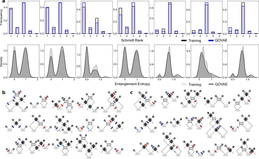
Fig. 2b displays 15 random samples of experiments from QOVAE-High and its training setups with lengths and . We can see the model has learned to generate experiments that have similar structure to the training experiments as both sets of samples have similar numbers of one and two photon devices as well as empty path devices.
We test if the distribution of entanglement of every bipartition is similar between experiments from the training data and the model. We generate experiments from the model and take training data and calculate all their entanglement entropies and Schmidt ranks in all seven bipartitions. We compare the distributions visually with a distribution plot for each of the seven bipartitions– we use kernel density estimators Scott 2015 to estimate the entanglement entropy densities and histograms for the Schmidt ranks (Fig. 2a).
We can see from the distribution plots in Fig. 2a that in the first four bipartitions (columns) the QOVAE-High successfully learns that the training entanglement has two modes (or peaks). For the last three bipartitions plots (last three columns), the QOVAE-High is able to learn that there is a single mode of entanglement in the training distribution. We notice that the QOVAE learns a heavier right tail than the training distribution.
From the results in Fig. 2 we conclude that the QOVAE has learned to match the training distribution of entanglement for every bipartition of the system and thus can learn distributions of entangled states.
3) The QOVAE learns a quasi-continuous embedding in terms of entanglement.
We demonstrate the smoothness of the latent space in terms of entanglement by testing if experiments that are close in the latent space have similar entanglement. First we perform spherical interpolations Shoemake 1985 from one latent representation of an experiment to another , decoding four experiments, at equally spaced steps on the interpolated path from .
We show three latent space interpolations in Figure 3, from different entanglement measures . The first interpolation shown in FIG 3 interpolates between experiments that do not produce entangled states– we encode two experiments with and generate experiments along the latent path between them. In this interpolation, the experiments decoded along the interpolation path remain in the unentangled () space like the initial and final experiments.
The the second is between experiments that both have and the last between one experiment with and another with . In the second interpolation, decoded experiment entanglement is within 0.5 of the initial and final experiments’ (). In the last interpolation, the entanglement of setups decoded along the path increases linearly from towards the final experiment’s entanglement of .
We also evaluate if nearby experiments in the latent space have similar entanglement properties by comparing the Euclidean distance between latent points and their absolute entanglement difference. We find that as the latent distance increases– the absolute entanglement difference increases and when the latent distance goes to 0– the difference in entanglement does as well. A plot of this relationship obtained by random sampling is shown in the supplementary. Thus, nearby experiments in the latent space are more likely to have similar entanglement properties than experiments further away.
Hence, the QOVAE learns a representation that encodes a measure of similarity between experiment and entanglement .
| Metric | QOVAE | TRAIN | QOVAE | TRAIN | QOVAE | TRAIN | QOVAE | TRAIN |
|---|---|---|---|---|---|---|---|---|
| Mode | ||||||||
| Mean | ||||||||
| SD | ||||||||
4) The QOVAE can be used to efficiently search for new highly entangled experiments and states.
We find that the QOVAE can efficiently search for new experiments with higher entanglement than random search and that the QOVAE is able to target and generate from specific levels of entanglement as well it can generate the most entangled training experiments with fewest devices, far faster than the random methods that produced them. Additionally, bayesian optimization can be used in the QOVAE’s latent space to exactly target specific states.
We report that the QOVAE can learn precise distributions of different levels of entanglement, defined by small intervals of entanglement with unity length. We train the QOVAE on four datasets with entanglement levels : 1) , 2) , 3) and 4) (using 14K, 11K, 18K and 10K setups respectively). The results in TABLE 1 show for each level of , the QOVAE perfectly matches the training mode of (the value most likely to be sampled) and learns the training mean within 1 standard error but over-estimates the of – confirming that the QOVAE seems to learn heavier right-tails for (Figure 2a). The model can perfectly capture the mode with no error. This is expected for a well trained QOVAE, while is continuous the training setups don’t all have different values – in fact one prominent value of dominates. For example, in the level , there are 677 different values in the 18K training setups but 40% of the 18K have . Each level of entanglement, basically defines a group of similar states– so the QOVAE can learn to target and generate states in these groups.
Next we train the QOVAE-high on the most difficult training experiments to find: some 5K out of 400K total that have the highest entanglement () and simplest structure (10 or less devices). The results show the QOVAE can learn to directly generate from this space as almost all– % of generated experiments have (and 10 or less devices). It also learns to produce the same mode () as the training data and within 1 standard error of the mean entanglement ( for ). Most importantly, using the QOVAE we can generate almost twice the number of these experiments with highest training entanglement and least number of devices – at a small fraction of the time (hours instead of days) it took to produce these experiments when building the training dataset. This demonstrates an important advantage of the QOVAE’s prior knowledge and is especially useful given how expensive entanglement is to calculate.
We can also target specific states by performing Bayesian optimization in the latent space, taking inspiration from Gómez-Bombarelli et al. 2018; Kusner et al. 2017, we use the target objective defined as . This is the fidelity between the target state and the state of experimental setup penalized by experiment length ( is the max experiment length) and is parameter that can be tuned in order to strengthen or weaken the device penalty. To perform Bayesian optimization (BO), we first train the QOVAE so that each training experiment has a latent vector defined by the mean of the encoder. After, we train a sparse Gaussian process to predict given its latent representation. Then we perform a set number of iterations of batched BO using the expected improvement heuristic– compiling the top scoring states.
As a toy example, we target the 2-dimensional 4 photon GHZ state
which is the state where each bipartition has Schmidt rank of 2 and entropy of 0.693– for a total entanglement measure of . We set the device penalty very small using and run BO for five iterations. We find a single quantum optics experiment that has the exact targeted state (). This experiment has 11 devices– 3 reflection devices, 5 beamsplitters, 3 holograms and 1 dove prism that are in the following sequence : .


6) The QOVAE learns an interpretable representation of quantum optics experiments.
We train the QOVAE-Low on three different datasets of experiments and plot its learned latent space– we discover that the QOVAE learns an intrepretible representation by structuring its learned representation according to the number and device order in its training experiments.
First we train the QOVAE-Low on equal distributions of and with . We directly plot the 2D latent space and interpret the latent space in terms of structure-property relations. We encode every training experiment into the latent space and color-code every latent point with its entanglement . We observe interesting patterns and distinct clusters of setups including a region that is unentangled (colored in violet), and another that is entangled as well as some mixed regions (see Fig. 4a. This is an interesting result, as the model is implicitly– not directly doing this since it is not provided the entanglement label. Instead, it must be placing its latent space according to experiment structure.
To understand exactly how, we analyse three different regions, one unentangled region A), one that shares entangled and unentangled states B) and one that contains only entangled states C).
In region A), we find three different clusters with no entangled states– but all setups have only four devices, while in region B) and C), all setups have nine devices. We color-coding the latent space by setup length, as shown in Fig. 4b, and find that the QOVAE encodes the training setups by number of optical devices. This shows a definitive correlation with entanglement.
However, the size of the setup cannot alone be responsible for the latent structure learned. After all, region B) and C) have the same number of elements, but B) contains both entangled and unentangled setups, while C) contains only entangled ones.
We analyse further and find, that the last element in every setup of region B) is always while in C) it is always . Therefore the QOVAE also structures its latent space by last setup element, we confirm this by color-coding all points by their final elements as shown in Fig. 4c.
This also explains why B) and C) have different entanglement : in region C), that the last element is which is needed to create entanglement, while in region B), the last device contributes nothing to entanglement so these experiments are less likely to be entangled.
We can further cluster all possible last elements into eight functional groups for instance, all holograms have the same effect on the entanglement property, so we can combine them to a single functional group. We plot the color-coded latent space according to functional groups in Fig. 4d and see additional grouping.
We conclude the QOVAE learns to structure its latent space according to experiment length and final device.
It seems there was pronounced correlation between length and entanglement in the last training subset of experiments. We train another QOVAE-Low on entirely entangled states and show this is not the defining structure the QOVAE uses to learn. This time we use 18K experiments evenly split between low entanglement and high entanglement . Similarly, in Fig. 5, it is apparent that the QOVAE structured its latent space by length– Fig. 5b and last device type– Fig. 5b as before, however there are clearer patterns and groups when plotting the functionality of last device type in Fig. 5d.
However, here we find that when we plot the entanglement in the latent space as shown in Fig. 5a this does not correlate with the length of the experiments as plotted in Fig. 5b or the last devices shown in Fig. 5c. Interestingly, there are visible regions of low entanglement and high entanglement in the latent space that is thus unexplained by structure. Likely the QOVAE is learning some additional information about the sequence structure or order that is responsible for this.
We further investigate how the QOVAE structures its latent space by removing length from the equation so the model can’t use it– in order to see additional insights into how the QOVAE structures its latent space and encodes the experiment sequence. We do this by training on 16K experiments that all have exactly 10 devices.
We discover that the QOVAE doesn’t structure its latent space using only the last device but will also use other information and devices in the experiment sequence, one clear example of this phenomenon is the latent space shown in Fig. 5e,f.
Here, the QOVAE-Low uses not just the last device but also the second last device to structure its latent space and group them in rows that are perpendicular to each other. It is clear the QOVAE is using the dimensions of its latent space to store information about specific devices in the sequence ordering. The QOVAE-Low uses the two dimensions it has in order to encode the last and second last experiment devices in groups in the latent space. This means QOVAE’s with higher dimensional latent spaces will be able to store more information about the devices at each location in the sequence ordering– using additional dimensions to encode and group devices.
This description provides us with a complete interpretation of our model’s latent representation and how it learns. With this new understanding, we can also explain results that we have observed in previous investigations. For example, we can explain exactly how the QOVAE can learn to generate from distributions of highly entangled states– it simply learns the distribution of device orderings that define its training experiments.
This distinguishes the QOVAE from other generative models applied to scientific domains– by directly training on the device sequence, we enable the QOVAE to learn a human-interpretable representation that could be practically exploited to design experiments. In doing so we provide one of the very few examples of opening up and successfully demystifying black-box deep generative models applied to complex scientific systems.
Conclusions
We presented the QOVAE which is the first deep generative model for the design of quantum optics hardware. Deep generative models are widely used but there has never been any investigation or understanding developed of their internal representation in a complex scientific domain. In a series of complex computational experiments, we investigated the QOVAE’s internal picture of the quantum world. The QOVAE was able to generate novel entangled experiments, learn distributions of entanglement and was shown to interpolate smoothly in its latent space– which can also be used to search efficiently for new highly entangled experiments and target specific distributions of entangled states. When plotting the QOVAE’s latent space we find complex internal structure, where the QOVAE learns a latent representation based on experiment length and device ordering. Our results go beyond designing new quantum optics– they tackle the question of interpretability and explainability of black-box models Rudin 2019; Gilpin et al. 2018 in a scientific domain. This is particularly promising since understanding what these model learn could lead to new computer-inspired scientific insights and discoveries.
Optical devices. In order to ensure the device toolbox is suitable, all elements are used in standard quantum optics laboratories Erhard et al. 2018; Erhard et al. 2020; Pan et al. 2012; Krenn et al. 2017; Malik et al. 2016, including the technique of entanglement by path identity Krenn et al. 2017. In addition, we use a device toolbox that is similar to others that have been used in related work on machine learning assisted design of quantum optics experiments Krenn et al. 2016; Melnikov et al. 2018; Adler et al. 2019.
In our current approach, we use linear optics devices, however, it would be straightforward to include any other nonlinear optics devices like four-wave mixers Wang et al. 2001 or optical parametric oscillators Giordmaine and Miller 1965. In addition, it would be possible to train the QOVAE on a universal set of optical devices with continuous parameters by discretizing the space of those parameters. However, the performance of the QOVAE needs to be investigated when including such devices. Furthermore, the QOVAE could still produce experiments that are challenging to implement in the lab.
Future work. In this paper, we provide an initial demonstration of the QOVAE and its potential– however, much further work needs to be done to truly assess and explore the use of its interpretable representation to investigate quantum optics experiments. Furthermore, while these investigations are exploratory, this work paves the way for many promising extensions that can be considered: conditional VAEs Kingma et al. 2014, where the encoder and decoder would be trained on both the experiment and entanglement or other information about the quantum state in order to generate experiments conditionally. Another interesting extension is the hierarchical VAE, which has layers of latent variables Sønderby et al. 2016; Zhao et al. 2017– these models have the ability to learn hierarchical features of the training data and have the potential to encode more information about experiment structure into their learned representation. Using Bayesian optimization in the QOVAE’s latent space it is possible to target many specific states but this is unlikely to be as efficient as domain specific methods Krenn et al. 2021. More interesting is how QOVAE learned to structure its latent representation– using its latent dimensions to independently encode the ordering of the experiment device sequence. Going forward, the most important future work is to figure out how this phenomenon can be exploited to develop new insights about quantum optics experiments and their design. Additionally, in future work, searching QOVAE’s latent space, different metrics may be useful for different states– for example like the GHZ state Bouwmeester et al. 1999 or W states Dür et al. 2000 or any other specific experimental setups for high dimensionally entangled states Erhard et al. 2020. In place of fidelity mean squared error between states can be used: where are basis ket probabilities of target and evaluated states. Another potential metric is the KL divergence between states . It is also possible to target absolutely maximally entangled states Cervera-Lierta et al. 2019; Helwig and Cui 2013 using the entanglement measure or the sum of the Schmidt rank vector components in place of fidelity.
Other applications. Indeed the insight from this work are applicable to generative models of molecules Kusner et al. 2017; Gómez-Bombarelli et al. 2018. Molecules and quantum optics experiments are similar discrete, structured objects– representable as graphs or sequences. If we treat quantum optics experiments are undirected we can even plot them as molecules by mapping devices to atoms– see the supplementary for a few examples. Based on how the QOVAE learns its representation we can infer that the ChemVAE Gómez-Bombarelli et al. 2018 could learn a representation that is more human-interpretable by using its dimensions to store information about the ordering of the SMILES string Weininger 1988. The QOVAE could, in principal, be directly be applied to other physical science domains, such as in the design of new quantum circuits for quantum computing. Currently, Noisy Intermediate-Scale Quantum (NISQ) computing algorithms Preskill 2018; Cerezo et al. 2021; Bharti et al. 2021 are promising candidates to surpasses the classical computational capabilities for numerous applications. Most of these approaches require good priors to explore efficiently and represent the space of parameters and solutions. The exponentially large Hilbert space formed by all possible quantum circuits makes this task computationally intractable when the structure-properties relation of these circuits is still not fully-understood. Only a few attempts to search this space have been made using genetic algorithms Giraldi et al. 2004; Yabuki and Iba 2000; Giraldi et al. 2004; Anand et al. 2021 which lack a sufficient prior. QOVAE’s ability to learn meaningful representations as understood by domain experts could provide insights about how the Hilbert space is organized within these parameterized quantum circuits. QOVAE learns an intrepretable representation of entanglement in quantum optics experiments. Our work with the QOVAE is an example in the physical sciences of opening the black-box of deep generative models to develop promising scientific insights.
Methods
.0.1 Encoder
Our encoder is a diagonal Gaussian whose parameters are a mapping from the data manifold to the latent space. Our data, the quantum optics experiments , are represented as a sequence with elements, each from a toolbox of possible devices,
where . First, consists of a convolutional neural network with 3 layers,
A single layer takes on the form
where is the convolution filter tensor which consists of filters each with length and features. Also the layer output is .
For the input layer, this is just the number of devices in the toolbox used to create any experiment. ReLU(·) is the element-wise rectified linear unit function and is the convolution operator which outputs a tensor with the following elements
where is the convolutional filter weight vector operating on the element (device) in the sequence (experiment).
The second component of the encoder is a MLP with three layers that maps the flattened output from the convolutional neural net. to the parameters of latent distribution
.0.2 Decoder
For the observation model, every data point is a sequence of devices from the element toolbox of possible device elements, thus we can model the data as independent categoricals whose mean vector is mapped from latent samples using a neural network,
where is the probability vector of each device in the toolbox. Our encoder outputs these probabilities as
First, consists of a three layer Recurrent neural network each with with Gated recurrent units (GRUs),
where is single layer MLP with a ReLU(.) activation. A single layer takes on the form
where are parameters of the GRU layer. The and are update and reset gate vectors, respectively, and is the sigmoid function. The input to the first GRU layer is the length sequence of vectors . The output of the RNN is mapped to the device probabilities using a softmax layer
.0.3 Training and data details
We manually performed an initial hyperparameter search for the QOVAE. We found an initial set of training hyperparameters using grid search. We found training on around 1600 epochs to produce better validation accuracy and ELBO values. We trained the QOVAE using stochastic gradient descent and the Adam optimizer Kingma and Welling 2013 with a low learning rate . Training was done using the KERAS machine learning package from tensorflow Abadi et al. 2016. All models were trained on a V100 GPU node on the Beluga supercomputer. The minibatch size grid was with an optimal batch size of 64. The model architecture is the same for all experiments with both models. We use grid search to search over the encoder and decoder architecture. For the convolutional layers– we search over filters with length . For the MLPs in both the decoder and encoder, we consider hidden units in each layer. For the GRU layer, we consider hidden states of size , and a 64 unit layer that maps to the GRU layers.
For new investigations, researchers can use the dataset provided to train the QOVAE, which has both and experiments. However, they can also produce new training datasets using the Melvin computer algorithm Krenn et al. 2016 with a different device toolbox of interest. For this, the sympy symbolic algebra is required to specify how each device changes the state of the system Nogueira 14. Melvin source code for creating new datasets is available. After training the QOVAE they can investigate the learned representation by plotting the latent vectors for each training experiment in a 2 or 3 dimensional space. If the QOVAE has a higher dimensional latent space they can plot specific dimensions or project the space into 2 or 3 dimensions. Based on this, the researcher can investigate how the latent space represents the training entanglement or use it to search for specific states as they see fit– either with random search or another search algorithm like the Bayesian optimization Nogueira 14 approach we use.
Data Availability
Training data is available:
https://github.com/danielflamshep/qovae/blob/main/setups.smi Nogueira 14.
Code Availability
Code is available:
https://github.com/danielflamshep/qovae Nogueira 14.
Acknowledgements
A.A.-G. acknowledge support from the Canada 150 Research Chairs Program, the Canada Industrial Research Chair Program, and from Google, Inc. in the form of a Google Focused Award. M.K. acknowledges support from the FWF (Austrian Science Fund) via the Erwin Schrödinger fellowship No. J4309.
Author Contributions
D.F.-S. conceived the overall project, developed the approach and wrote the paper. D.F.-S. and T.W. designed and performed investigations. A.C.L. provided technical advice. X.G. provided technical advice and wrote the entanglement calculation code. M.K. built the dataset, provided technical advice and helped design the intrepretibility investigation and analysed experiments. A.A.-G. led the project and provided overall directions. All authors participated in preparing the manuscript.
Competing Interests
The authors declare that there are no competing interests.
references
References
- Schrödinger (1935) E. Schrödinger, “Discussion of probability relations between separated systems,” Mathematical Proceedings of the Cambridge Philosophical Society 31, 555 (1935).
- Einstein et al. (1935) A. Einstein, B. Podolsky, and N. Rosen, “Can quantum-mechanical description of physical reality be considered complete?” Physical review 47, 777 (1935).
- Bell (1964) J. S. Bell, “On the einstein podolsky rosen paradox,” Physics Physique Fizika 1, 195–200 (1964).
- Giustina et al. (2015) M. Giustina, M. A. Versteegh, S. Wengerowsky, J. Handsteiner, A. Hochrainer, K. Phelan, F. Steinlechner, J. Kofler, J.-Å. Larsson, C. Abellán, et al., “Significant-loophole-free test of bell’s theorem with entangled photons,” Physical review letters 115, 250401 (2015).
- Shalm et al. (2015) L. K. Shalm, E. Meyer-Scott, B. G. Christensen, P. Bierhorst, M. A. Wayne, M. J. Stevens, T. Gerrits, S. Glancy, D. R. Hamel, M. S. Allman, et al., “Strong loophole-free test of local realism,” Physical review letters 115, 250402 (2015).
- Bong et al. (2020) K.-W. Bong, A. Utreras-Alarcón, F. Ghafari, Y.-C. Liang, N. Tischler, E. G. Cavalcanti, G. J. Pryde, and H. M. Wiseman, “A strong no-go theorem on the wigner’s friend paradox,” Nature Physics 16, 1199 (2020).
- Yin et al. (2017) J. Yin, Y. Cao, Y.-H. Li, J.-G. Ren, S.-K. Liao, L. Zhang, W.-Q. Cai, W.-Y. Liu, B. Li, H. Dai, et al., “Satellite-to-ground entanglement-based quantum key distribution,” Physical review letters 119, 200501 (2017).
- Peruzzo et al. (2014) A. Peruzzo, J. McClean, P. Shadbolt, M.-H. Yung, X.-Q. Zhou, P. J. Love, A. Aspuru-Guzik, and J. L. O’brien, “A variational eigenvalue solver on a photonic quantum processor,” Nature communications 5, 1 (2014).
- Paesani et al. (2019) S. Paesani, Y. Ding, R. Santagati, L. Chakhmakhchyan, C. Vigliar, K. Rottwitt, L. K. Oxenløwe, J. Wang, M. G. Thompson, and A. Laing, “Generation and sampling of quantum states of light in a silicon chip,” Nature Physics 15, 925 (2019).
- Zhong et al. (2020) H.-S. Zhong, H. Wang, Y.-H. Deng, M.-C. Chen, L.-C. Peng, Y.-H. Luo, J. Qin, D. Wu, X. Ding, Y. Hu, et al., “Quantum computational advantage using photons,” Science 370, 1460 (2020).
- Wang et al. (1991) L. Wang, X. Zou, and L. Mandel, “Induced coherence without induced emission,” Physical Review A 44, 4614 (1991).
- Herzog et al. (1994) T. Herzog, J. Rarity, H. Weinfurter, and A. Zeilinger, “Frustrated two-photon creation via interference,” Physical review letters 72, 629 (1994).
- Menssen et al. (2017) A. J. Menssen, A. E. Jones, B. J. Metcalf, M. C. Tichy, S. Barz, W. S. Kolthammer, and I. A. Walmsley, “Distinguishability and many-particle interference,” Physical review letters 118, 153603 (2017).
- Feng et al. (2021) L.-T. Feng, M. Zhang, D. Liu, Y.-J. Cheng, G.-P. Guo, D.-X. Dai, G.-C. Guo, M. Krenn, and X.-F. Ren, “Observation of nonlocal quantum interference between the origins of a four-photon state in a silicon chip,” arXiv:2103.14277 (2021).
- Krenn et al. (2020) M. Krenn, M. Erhard, and A. Zeilinger, “Computer-inspired quantum experiments,” Nature Reviews Physics 2, 649 (2020).
- Krenn et al. (2016) M. Krenn, M. Malik, R. Fickler, R. Lapkiewicz, and A. Zeilinger, “Automated search for new quantum experiments,” Physical Review Letters 116 (2016), 10.1103/physrevlett.116.090405.
- Krenn et al. (2021) M. Krenn, J. Kottmann, N. Tischler, and A. Aspuru-Guzik, “Conceptual understanding through efficient automated design of quantum optical experiments,” Physical Review X 11, 031044 (2021).
- Knott (2016) P. Knott, “A search algorithm for quantum state engineering and metrology,” New Journal of Physics 18, 073033 (2016).
- Nichols et al. (2019) R. Nichols, L. Mineh, J. Rubio, J. C. Matthews, and P. A. Knott, “Designing quantum experiments with a genetic algorithm,” Quantum Science and Technology 4, 045012 (2019).
- O’Driscoll et al. (2019) L. O’Driscoll, R. Nichols, and P. A. Knott, “A hybrid machine learning algorithm for designing quantum experiments,” Quantum Machine Intelligence 1, 5 (2019).
- Melnikov et al. (2018) A. A. Melnikov, H. Poulsen Nautrup, M. Krenn, V. Dunjko, M. Tiersch, A. Zeilinger, and H. J. Briegel, “Active learning machine learns to create new quantum experiments,” Proceedings of the National Academy of Sciences 115, 1221–1226 (2018).
- Arrazola et al. (2019) J. M. Arrazola, T. R. Bromley, J. Izaac, C. R. Myers, K. Brádler, and N. Killoran, “Machine learning method for state preparation and gate synthesis on photonic quantum computers,” Quantum Science and Technology 4, 024004 (2019).
- Salakhutdinov (2015) R. Salakhutdinov, “Learning deep generative models,” Annual Review of Statistics and Its Application 2, 361 (2015).
- Razavi et al. (2019) A. Razavi, A. v. d. Oord, and O. Vinyals, “Generating diverse high-fidelity images with vq-vae-2,” arXiv preprint arXiv:1906.00446 (2019).
- Bowman et al. (2015) S. R. Bowman, L. Vilnis, O. Vinyals, A. M. Dai, R. Jozefowicz, and S. Bengio, “Generating sentences from a continuous space,” arXiv preprint arXiv:1511.06349 (2015).
- Semeniuta et al. (2017) S. Semeniuta, A. Severyn, and E. Barth, “A hybrid convolutional variational autoencoder for text generation,” arXiv preprint arXiv:1702.02390 (2017).
- Roberts et al. (2018) A. Roberts, J. Engel, C. Raffel, C. Hawthorne, and D. Eck, in International Conference on Machine Learning (PMLR, 2018) pp. 4364–4373.
- Sanchez-Lengeling and Aspuru-Guzik (2018) B. Sanchez-Lengeling and A. Aspuru-Guzik, “Inverse molecular design using machine learning: Generative models for matter engineering,” Science 361, 360 (2018).
- Kingma and Welling (2013) D. P. Kingma and M. Welling, “Auto-encoding variational bayes,” arXiv preprint arXiv:1312.6114 (2013).
- Gómez-Bombarelli et al. (2018) R. Gómez-Bombarelli, J. N. Wei, D. Duvenaud, J. M. Hernández-Lobato, B. Sánchez-Lengeling, D. Sheberla, J. Aguilera-Iparraguirre, T. D. Hirzel, R. P. Adams, and A. Aspuru-Guzik, “Automatic chemical design using a data-driven continuous representation of molecules,” ACS central science 4, 268 (2018).
- Samanta et al. (2020) B. Samanta, A. De, G. Jana, V. Gómez, P. K. Chattaraj, N. Ganguly, and M. Gomez-Rodriguez, “Nevae: A deep generative model for molecular graphs,” Journal of machine learning research. 2020 Apr; 21 (114): 1-33 (2020).
- Jin et al. (2018) W. Jin, R. Barzilay, and T. Jaakkola, “Junction tree variational autoencoder for molecular graph generation,” arXiv preprint arXiv:1802.04364 (2018).
- Flam-Shepherd et al. (2021) D. Flam-Shepherd, T. C. Wu, and A. Aspuru-Guzik, “Mpgvae: Improved generation of small organic molecules using message passing neural nets,” Machine Learning: Science and Technology (2021).
- Jin et al. (2020) W. Jin, R. Barzilay, and T. Jaakkola, “Hierarchical generation of molecular graphs using structural motifs,” International Conference on Machine Learning , 4839 (2020).
- Yao et al. (2021) Z. Yao, B. Sánchez-Lengeling, N. S. Bobbitt, B. J. Bucior, S. G. H. Kumar, S. P. Collins, T. Burns, T. K. Woo, O. K. Farha, R. Q. Snurr, et al., “Inverse design of nanoporous crystalline reticular materials with deep generative models,” Nature Machine Intelligence 3, 76 (2021).
- Liu et al. (2018) Q. Liu, M. Allamanis, M. Brockschmidt, and A. Gaunt, in Advances in Neural Information Processing Systems (2018) pp. 7795–7804.
- Bengio et al. (2013) Y. Bengio, A. Courville, and P. Vincent, “Representation learning: A review and new perspectives,” IEEE transactions on pattern analysis and machine intelligence 35, 1798 (2013).
- Higgins et al. (2016) I. Higgins, L. Matthey, A. Pal, C. Burgess, X. Glorot, M. Botvinick, S. Mohamed, and A. Lerchner, “beta-vae: Learning basic visual concepts with a constrained variational framework,” (2016).
- Iten et al. (2020) R. Iten, T. Metger, H. Wilming, L. del Rio, and R. Renner, “Discovering physical concepts with neural networks,” Physical Review Letters 124 (2020), 10.1103/physrevlett.124.010508.
- Bouwmeester et al. (1999) D. Bouwmeester, J.-W. Pan, M. Daniell, H. Weinfurter, and A. Zeilinger, “Observation of three-photon greenberger-horne-zeilinger entanglement,” Physical Review Letters 82, 1345–1349 (1999).
- Yao et al. (2012) X.-C. Yao, T.-X. Wang, P. Xu, H. Lu, G.-S. Pan, X.-H. Bao, C.-Z. Peng, C.-Y. Lu, Y.-A. Chen, and J.-W. Pan, “Observation of eight-photon entanglement,” Nature photonics 6, 225 (2012).
- Allen et al. (1992) L. Allen, M. W. Beijersbergen, R. J. C. Spreeuw, and J. P. Woerdman, “Orbital angular momentum of light and the transformation of laguerre-gaussian laser modes,” Physical Review A 45, 8185–8189 (1992).
- Romero et al. (2012) J. Romero, D. Giovannini, S. Franke-Arnold, S. M. Barnett, and M. J. Padgett, “Increasing the dimension in high-dimensional two-photon orbital angular momentum entanglement,” Physical Review A 86 (2012), 10.1103/physreva.86.012334.
- Krenn et al. (2014) M. Krenn, M. Huber, R. Fickler, R. Lapkiewicz, S. Ramelow, and A. Zeilinger, “Generation and confirmation of a (100 x 100)-dimensional entangled quantum system,” Proceedings of the National Academy of Sciences 111, 6243–6247 (2014).
- Erhard et al. (2018) M. Erhard, M. Malik, M. Krenn, and A. Zeilinger, “Experimental greenberger–horne–zeilinger entanglement beyond qubits,” Nature Photonics 12, 759 (2018).
- Luo et al. (2019) Y.-H. Luo, H.-S. Zhong, M. Erhard, X.-L. Wang, L.-C. Peng, M. Krenn, X. Jiang, L. Li, N.-L. Liu, C.-Y. Lu, A. Zeilinger, and J.-W. Pan, “Quantum teleportation in high dimensions,” Physical review letters 123, 070505 (2019).
- Leach et al. (2002) J. Leach, M. J. Padgett, S. M. Barnett, S. Franke-Arnold, and J. Courtial, “Measuring the orbital angular momentum of a single photon,” Physical Review Letters 88 (2002), 10.1103/physrevlett.88.257901.
- Huber and De Vicente (2013) M. Huber and J. I. De Vicente, “Structure of multidimensional entanglement in multipartite systems,” Physical review letters 110, 030501 (2013).
- Meurer et al. (2017) A. Meurer, C. P. Smith, M. Paprocki, O. Čertík, S. B. Kirpichev, M. Rocklin, A. Kumar, S. Ivanov, J. K. Moore, S. Singh, et al., “Sympy: symbolic computing in python,” PeerJ Computer Science 3, e103 (2017).
- Hamma et al. (2012) A. Hamma, S. Santra, and P. Zanardi, “Quantum entanglement in random physical states,” Physical review letters 109, 040502 (2012).
- Adler et al. (2019) T. Adler, M. Erhard, M. Krenn, J. Brandstetter, J. Kofler, and S. Hochreiter, “Quantum optical experiments modeled by long short-term memory,” arXiv preprint arXiv:1910.13804 (2019).
- Li et al. (2018) Y. Li, O. Vinyals, C. Dyer, R. Pascanu, and P. Battaglia, “Learning deep generative models of graphs,” arXiv preprint arXiv:1803.03324 (2018).
- Scott (2015) D. W. Scott, Multivariate density estimation: theory, practice, and visualization (John Wiley & Sons, 2015).
- Shoemake (1985) K. Shoemake, in Proceedings of the 12th annual conference on Computer graphics and interactive techniques (1985) pp. 245–254.
- Kusner et al. (2017) M. J. Kusner, B. Paige, and J. M. Hernández-Lobato, “Grammar variational autoencoder,” arXiv preprint arXiv:1703.01925 (2017).
- Rudin (2019) C. Rudin, “Stop explaining black box machine learning models for high stakes decisions and use interpretable models instead,” Nature Machine Intelligence 1, 206 (2019).
- Gilpin et al. (2018) L. H. Gilpin, D. Bau, B. Z. Yuan, A. Bajwa, M. Specter, and L. Kagal, in 2018 IEEE 5th International Conference on data science and advanced analytics (DSAA) (IEEE, 2018) pp. 80–89.
- Erhard et al. (2020) M. Erhard, M. Krenn, and A. Zeilinger, “Advances in high-dimensional quantum entanglement,” Nature Reviews Physics 2, 365 (2020).
- Pan et al. (2012) J.-W. Pan, Z.-B. Chen, C.-Y. Lu, H. Weinfurter, A. Zeilinger, and M. Żukowski, “Multiphoton entanglement and interferometry,” Reviews of Modern Physics 84, 777 (2012).
- Krenn et al. (2017) M. Krenn, A. Hochrainer, M. Lahiri, and A. Zeilinger, “Entanglement by path identity,” Physical Review Letters 118, 080401 (2017).
- Malik et al. (2016) M. Malik, M. Erhard, M. Huber, M. Krenn, R. Fickler, and A. Zeilinger, “Multi-photon entanglement in high dimensions,” Nature Photonics 10, 248 (2016).
- Wang et al. (2001) L. Wang, C. Hong, and S. Friberg, “Generation of correlated photons via four-wave mixing in optical fibres,” Journal of optics B: Quantum and semiclassical optics 3, 346 (2001).
- Giordmaine and Miller (1965) J. A. Giordmaine and R. C. Miller, “Tunable coherent parametric oscillation in linb o 3 at optical frequencies,” Physical Review Letters 14, 973 (1965).
- Kingma et al. (2014) D. P. Kingma, S. Mohamed, D. J. Rezende, and M. Welling, in Advances in neural information processing systems (2014) pp. 3581–3589.
- Sønderby et al. (2016) C. K. Sønderby, T. Raiko, L. Maaløe, S. K. Sønderby, and O. Winther, “Ladder variational autoencoders,” Advances in neural information processing systems 29 (2016).
- Zhao et al. (2017) S. Zhao, J. Song, and S. Ermon, “Learning hierarchical features from generative models,” arXiv preprint arXiv:1702.08396 (2017).
- Dür et al. (2000) W. Dür, G. Vidal, and J. I. Cirac, “Three qubits can be entangled in two inequivalent ways,” Physical Review A 62, 062314 (2000).
- Cervera-Lierta et al. (2019) A. Cervera-Lierta, J. I. Latorre, and D. Goyeneche, “Quantum circuits for maximally entangled states,” Physical Review A 100, 022342 (2019).
- Helwig and Cui (2013) W. Helwig and W. Cui, “Absolutely maximally entangled states: existence and applications,” arXiv preprint arXiv:1306.2536 (2013).
- Weininger (1988) D. Weininger, “Smiles, a chemical language and information system. 1. introduction to methodology and encoding rules,” Journal of chemical information and computer sciences 28, 31 (1988).
- Preskill (2018) J. Preskill, “Quantum computing in the nisq era and beyond,” Quantum 2, 79 (2018).
- Cerezo et al. (2021) M. Cerezo, A. Arrasmith, R. Babbush, S. C. Benjamin, S. Endo, K. Fujii, J. R. McClean, K. Mitarai, X. Yuan, L. Cincio, and P. J. Coles, “Variational quantum algorithms,” Nature Reviews Physics , 1 (2021).
- Bharti et al. (2021) K. Bharti, A. Cervera-Lierta, T. H. Kyaw, T. Haug, S. Alperin-Lea, A. Anand, M. Degroote, H. Heimonen, J. S. Kottmann, T. Menke, et al., “Noisy intermediate-scale quantum (nisq) algorithms,” arXiv preprint arXiv:2101.08448 (2021).
- Giraldi et al. (2004) G. A. Giraldi, R. Portugal, and R. N. Thess, “Genetic algorithms and quantum computation,” arXiv preprint cs/0403003 (2004).
- Yabuki and Iba (2000) T. Yabuki and H. Iba, in Late Breaking Papers at the 2000 Genetic and Evolutionary Computation Conference (Citeseer, 2000) pp. 421–425.
- Anand et al. (2021) A. Anand, M. Degroote, and A. Aspuru-Guzik, “Natural evolutionary strategies for variational quantum computation,” Machine Learning: Science and Technology (2021).
- Hoffman et al. (2013) M. D. Hoffman, D. M. Blei, C. Wang, and J. Paisley, “Stochastic variational inference.” Journal of Machine Learning Research 14 (2013).
- Abadi et al. (2016) M. Abadi, P. Barham, J. Chen, Z. Chen, A. Davis, J. Dean, M. Devin, S. Ghemawat, G. Irving, M. Isard, et al., in 12th USENIX symposium on operating systems design and implementation (OSDI 16) (2016) pp. 265–283.
- Nogueira (14 ) F. Nogueira, “Bayesian Optimization: Open source constrained global optimization tool for Python,” (2014–).
- Nogueira (14 ) Zenodo, “python code and data for training and sampling from models,” (2021–).
Supplementary Materials
| Device | Token | Visual | Operation | Operator |
|---|---|---|---|---|
| Down Conversion | ||||
| Beam Splitter | ||||
| Mirror | ||||
| Dove Prism | ||||
| Hologram | ||||
| Hologram | ||||
.1 The quantum state
.1.1 The quantum system
We are investigating multipartite entanglement in a four photon system with two pairs of OAM-entangled photons. The state is represented by the OAM of the photon which is its orbital angular momentum. Each maximally entangled quantum optics experimental setup will produce some state which lives in the hilbert space defined by the tensor product of the individual subsystems defined by photons given by
| (1) |
where we can define a general state in the system as a superposition of the basis kets as defined
| (2) | ||||
| (3) |
where are the OAM quantum number of the photon, OAM states provide a suitable physical realisation of multilevel qudit systems which have been shown to improve the robustness of quantum key distribution schemes. In general, photon OAM states take on discrete integer values with OAM . A proof-of-principle experiment with 7 OAM modes from has been demonstrated Mirhosseini_2015 .
where is the maximal OAM number that can be reached by the setup, and is the smallest that can be reached. This means each OAM quantum number can take on a possible discrete values and since the system consists of four photons ()the dimension of the Hilbert space is and each basis ket lives in
What states can be generated. Based on the states produced in the training data using the devices in Table 2 the OAM values don’t go above and the coefficients of basis kets can take on possible values :
where is a real prefactor from normalization.
.1.2 Initial State and SPDC
Here, the initial state is created by a double spontaneous parametric down-conversion (SPDC) process. SPDC is a widespread source for the experimental generation of photon pairs. Multiple SPDC processes can be used to produce multipartite entanglement, as it is well known for the case of two-dimensional polarization entanglement Bouwmeester et al. 1999; Yao et al. 2012. However, instead of polarization, we are using the OAM of photons Allen et al. 1992; Dada_2011; Romero et al. 2012; Krenn et al. 2014, which is a discrete high-dimensional degree of freedom based on the spatial structure of the photonic wave function
The input state of example 1 is a double-emission from SPDC, which leads to the initial state with general form :
| (4) |
with being the highest order of SPDC considered, with photon pairs and . is a normalization constant. During creation of the dataset we only consider with initial state
| (5) |
This is the unnormalized state produced from the two initial SPDC devices, when we visualize the experiments we depict this as two grey rectangles to depict the crystal as in Figure 6.
.2 State and entanglement calculations
To calculate the state of some experimental setup that has an initial state from the SPDC process we define the set of operations the state will undergo by extracting the operators defined from the sequence of optical devices that define the experiment. For each we have a corresponding operator that changes the state by acting on it according to Table 2. Each device changes the state in the order defined by the sequence of the experiment and leads to a state which we then square collect four dimensionally entangled terms then normalize : . If there are no four particle or the state consists of one of the basis kets then the experiment is unentangled.
Now we must quantify and calculate the entanglement in our system using the systems final state calculated in the previous paragraph and in Algorithm 1. Since our state lives in the hilbert space as
| (6) |
the density matrix of the system is given by
| (7) |
We need to keep track of the four reduced density matrices for each subsystem or photon . For example in the case of we can calculate by tracing out the other subsystems. Explicitly :
| (8) |
The other three can be calculated in similar fashion. We also need to keep track of the three reduced density matrices for each photon pair . Similarly in in the case of the photon pair we can calculate by tracing out the other subsystems.
| (9) |
The other two can be calculated in similar fashion. we are interested in two main vectors quantifying the entanglement of the system ; 1) the von neumann entropy vector and 2) the Schmidt rank vector where
| (10) |
To explain the SRV, consider the simpler case of 3 particles and the state which has a SRV of (4,2,2)
| (11) |
Here, the first particle is four-dimensionally entangled with the other two parties, whereas particle two and three are both only two dimensionally entangled with the rest. Also, is the von neumann entropy given by
| (12) |
where are the eigenvalues of the quantum system .
Entanglement entropy is a measure of the degree of quantum entanglement between two subsystems constituting a two-part composite quantum system. Given a pure bipartite quantum state of the composite system, the reduced density matrix describes the state of a subsystem. The entropy of entanglement is the Von Neumann entropy of the reduced density matrix for any of the subsystems. If it is non-zero, the subsystem is in a mixed state and the two subsystems are entangled.
We define our entanglement measure as the sum of all the entanglement entropies of all bipartitions of the system
| (13) |
A bipartition of the system is a partition which divide the system into two parts and , containing and particles respectively with supposing the quantum system consist of particles. Bipartite entanglement entropy is defined with respect to this bipartition.
.3 Example state calculation
The state calculation is automated using symbolic algebra from the sympy python package Meurer et al. 2017. For demonstration purposes let’s consider an example state calculation of a simple quantum optics experiment defined in Fig 8 the sequence of devices in the experiment operate on the state through the sequence of operators
| (14) |
starting with the initial state We apply each operator in order to find the final state given by
| (15) |
The first device in the setup is a beamsplitter on photon path b and c with operator acting on the initial state replacing and kets with their superposition as
| (16) |
next the device will add 1 OAM to all kets, so that the two zero OAM for photon b become Then applying device
| (17) |
Then applying device and device we flip c and add a prefactor as well as increase the OAM of kets . Then we square the state and normalize:
we are left with the following terms that contribute to 4 dimensional entanglement :
| (18) |
.4 Further experiments
| Training data upper-bound | |||
|---|---|---|---|
| QOVAE 95 PT | |||
| TRAIN 95 PT | |||
| Samples | |
|---|---|
|
Training Samples |
|
|
QOVAE Samples |
 |