Relaxation of the Ising spin system coupled to a bosonic bath and the time dependent mean field equation
Abstract
The Ising model doesn’t have a strictly defined dynamics, only a spectrum. There are different ways to equip it with a time dependence e.g. the Glauber or the Kawasaki dynamics, which are both stochastic, but it means there is a master equation which can also describes their dynamics. We present a Gluber-type master equation derived from the Redfield equation, where the spin system is coupled to a bosonic bath. We derive a time dependent mean field equation which describes the relaxation of the spin system at finite temperature. Using the fully connected, uniform Ising model the relaxation time will be studied, and the critical behaviour around the critical temperature. The master equation shows the finite size effects, and the mean field equation the thermodynamic limit.
I Introduction
Spin models are versatile, because they are simple, yet able to demonstrate fundamental phenomenons, like phase transition Ising 1925; Onsager 1944; Baxter 1982. Many complex physical models can be reduced to a simple Ising or Heisenberg model, like electron and nuclear spins Sólyom 2007, and even social situations Mézard et al. 1987. It is also important in modern applied physics since one brach of adiabatic quantum computers - like the D-Wave system Harris et al. 2018 - are based on finding the global minimum of an artificial spin system Farhi et al. 2000; Roland and Cerf 2002.
The Ising model is defined via its energy or in the quantum case, where it is often called Heisenberg model, via its Hamiltonian operator. The former do not have a natural dynamics, and although the latter has one, i.e. the Schrödinger or the Heisenberg equation, it is not always what we want. For example if we want our system to converge to the Boltzmann distribution, then the Schrödinger equation is not enough.
To describe such a system we must use the tools of open quantum systems Breuer et al. 2002; Schaller 2014 like the Redfield Redfield 1965 and the Lindblad equation Lindblad 1976. These equations have countless applications in quantum biology Rebentrost et al. 2009; Guerreschi et al. 2012, quantum optics Breuer et al. 2002, cold atomic gases Sieberer et al. 2016, chemical physics Oppenheim et al. 1977 and besides it is also relevant in quantum computing Vacchini and Breuer 2010; Davies 1976; Leggett et al. 1987.
Quantum dissipation and relaxation of spin systems in a bosonic bath and in magnetic field have been investigated by many authors. Albash and Lidar 2015; Takada and Nishimori 2016; Cugliandolo et al. 2002; Sinha and Dattagupta 2013. The interaction between an adiabatic computer and its enviroment is meant to be small, so the weak coupling Lindblad equation will be used, but of course there are improved methods to describe open quantum systems, like slippage initial condition Suárez et al. 1992; Gaspard and Nagaoka 1999, Nakajima-Zwanzig equation Nakajima 1958; Zwanzig 1960 or the polaron transformation Wang et al. 2015.
The structure of this paper is the following. In section II we present a Glauber-type master equation based on the Redfield equation. In section III we investigate the temperature dependence of the eigenvalues of the transition matrix, because they contain relevant informations on the time scales of the system, e.g. the relaxation time. We give an upper bound to the smallest nonzero eigenvalue, then in section IV the dynamics of the uniform, fully connected Ising model is investigated, and we show that the relaxation time diverges in the thermodynamic limit as the temperature approaches the critical temperature. In section V a time dependent mean field equation is derived from the master equation, which will be tested in section VI using the uniform Ising model.
II Master equation of quantum Ising system
In general if a system is connected to a bath, than its Hamiltonian operator is
| (1) |
where acts only on the system of interest, only on the bath, and is the interaction between the two subsystems, and it can be written as , where and are system and bath operators respectively. The dynamics of the total system is described by the von Neumann equation.
| (2) |
If the interaction between the system and the bath is small, than after the Born and the Markov approximation an effective equation can be derived to the density matrix of the system of interest ().
| (3) |
where , is in interaction picture, is the bath correlation function, and h.c means hermitian conjugate. This is the Redfield equation in weak-coupling limit Redfield 1965. After the so called secular or rotating wave approximation one can get to equation
| (4) |
where and is the eigenvector of with eigenvalue Breuer et al. 2002. is the Lamb shift Hamiltonian, which is usually small, so we will neglect it, and is the Fourier transform of the bath correlation function.
| (5) |
There are two common bosonic bathes: the bath of phonons and the bath of photons. For phonons , which is called Ohmic case and for photons , which is a super-Ohmic case. The frequency is the cutoff frequency. If we assume, that is large compared to the energy distances of the system, than . Figure 1 shows the main features of the two functions. The main difference is that is strictly increasing and , but is non-monotonic, and . In the easiest case .


The advantage of the weak-coupling limit is that a master equation can be derived to the diagonal elements of .
| (6) |
where , and .
The system converges to the Boltzmann distribution if satisfies the detailed balance condition i.e. . Both the Ohmic and the super-Ohmic bath satisfy it, because
| (7) |
If the system of interest is the Ising model, then the Hamiltonian is
| (8) |
where is the Pauli z-matrix and the corresponding eigenvectors are
| (9) |
with eigenenergies
| (10) |
The easiest way to couple the system to the bath is via a Pauli matrix i.e. . Using in the interacion instead of would not give any relevant dynamics, since the system and the interaction Hamiltonians would commute. The peculiarity of this system is that the populations decouple even without the secular approximation.
The operator acting on only flips the th spin, so the matrix element is
| (11) |
With Eq. (6) and (11) we have a dynamics for the Ising model.
| (12) |
where is the transition matrix. This matrix is temperature dependent, and it has at least one zero eigenvalue, which is the eigenvalue of the equilibrium distribution:
| (13) |
For constant temperature the general solution of (12) is
| (14) |
where s are the right, and s are the left eigenvectors of with eigenvalues. All the s are nonnegative. If the system is ergodic, then there is only one zero eigenvalue, and the other s are positive. Let the smallest positive be and the largest be . The relaxation time is . This is the time scale in which all but the equilibrium mode dies out. The other relevant time scale is , which is the characteristic time of the fastest mode. If for example this spin system is a quantum computer, then the fastest mode is the more important, because if the computation is slower than this time scale, then the enviroment isn’t neglectable. In other words is important if we want the system to relax thermally, and is important if we want to avoid any thermal influence.
III Temperature dependence of the eigenvalues
Both the smallest and the largest eigenvalue carry relevant information, and since is temperature dependent and are too.
At high temperature we can determine the temperature dependence of all s by simply Taylor expanding for small .
| (15) |
where in the Ohmic, and in the super-Ohmic case. The transition matrix inherits this temperature dependence: , and hence .
In spite of the high temperature limit, where the elements of the dynamical matrix diverges, in the low temperature limit they converge.
| (16) |
It means all the eigenvalues also converge. As a consequence we can’t slow down arbitrary all the modes by reducing the temperature. We have an upper limit in time for the quantum computing. Of course this calculation is valid only for a time independent system, but the main features apply to more general cases.
Without external magnetic field () at zero temperature the equilibrium Boltzmann distribution prefers only the two spin configurations with the lowest energies:
| (17) |
where and are the ground states. At zero temperature there is one more eigenvector with zero eigenvalue:
| (18) |
The question is how behaves at low temperature. We can give an upper bound. First let us introduce the following symmetric matrix:
| (19) |
This transformation doesn’t affect the eigenvalues, and the eigenvectors transform like
| (20) |
Since is symmetric its right and left eigenvectors are the same, and now the variational method applies to it:
| (21) |
where is an arbitrary vector with , and it must be perpendicular to the equilibrium vector ( ), because is the second smallest eigenvalue of . Let . Then accordig to (21)
| (22) | ||||
where is the Hamming distance, and the symmetry was used. In the bosonic bath
| (23) |
where . At low temperature this is the sum of some functions, so can be estimated from above with an exponential function.
Figure 2 shows , and (the upper bound) for a , ferromagnetic, 2D Ising model with Ohmic bath. The dashed vertical line marks the critical temperature (). The left figure is in log-log scale, where we can see, that at low temperature the eigenvalues has a temperature dependence, and converges, and the right figure with lin-log scale shows, that goes to zero exponentially.
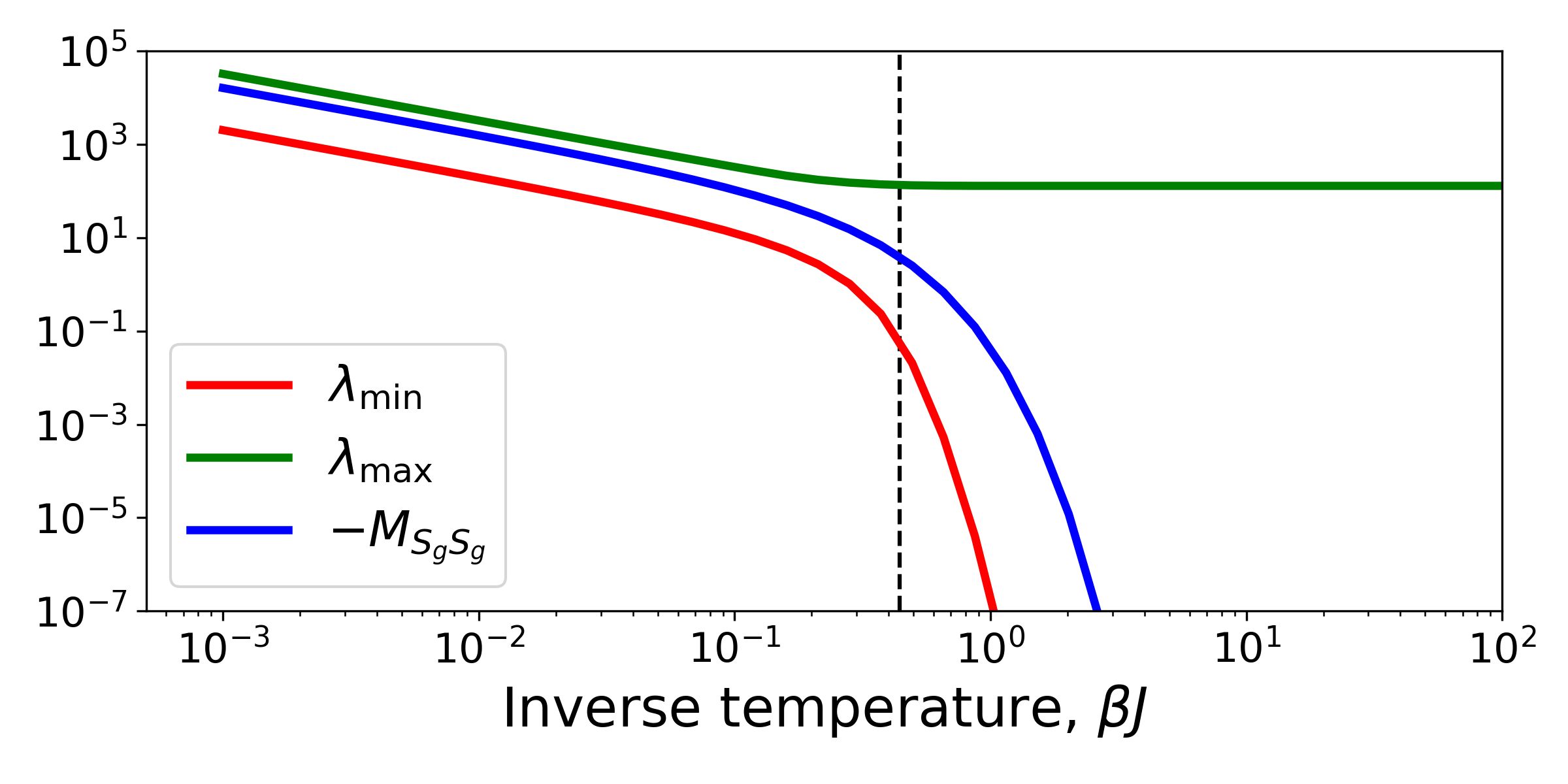
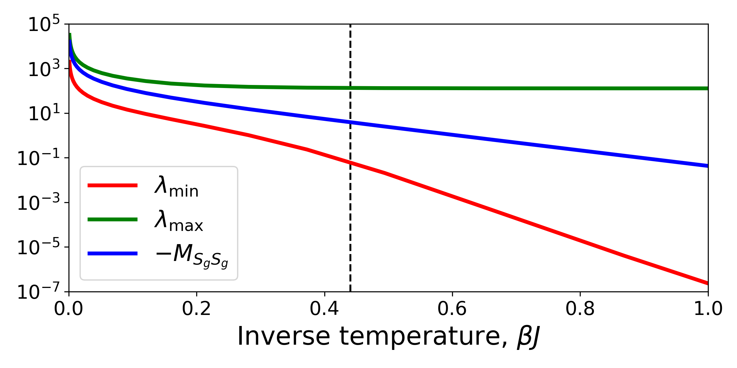
2D, ferromagnetic, Ising model, Ohmic bath, ,
IV Eigenvalues of the uniform Ising model
The matrices are large, therefore we can’t see how the eigenvalues behave at the thermodinamic limit. However the uniform, fully connected Ising model is so symmetric, that an effective equation can be derived, which has the same relaxation time as the original equation.
The energy of the model is
| (24) |
The factor is to keep the energy extensive and . Given an microstate, it consists of spins with and spins with . The number of spins is constant, i.e. . The energy of such a configuration is
| (25) |
If is fixed, then the energy is the function of only . The symmetry of the system is that we can perturb the spins any way, the energy and the matrix remains the same. If in the dynamic the initial condition also has this symmetry, then the will inherit this property. The slowest mode propagates between the two deepest valley of the energy landscape, which are the and . Assume that initially , and we want to determine relaxation time, where . Since both the equations and the initial condition has the permutation symmetry all the probabilities, which has the same up spin has the same value, e.g. for 3 spins . The probability can only flow between spin configurations if the Hamming distance between them is 1. Let us introduce the following probabilities:
| (26) |
where the prime denotes that only such configurations count where there are up spin. We can give a closed set of differential equations which only contain this new probabilities.
| (27) | ||||
where . This master equation has only variables instead of , thus easy to simulate for large systems. A comparison between the quantum and the thermal simulated annealing of the fully connected Ising model was investigated by Wauters et al. using a similar reduced master equation Wauters et al. 2017. Equation (27) has the form
| (28) |
and we want to determine the lowest (nonzero) eigenvalue of , which is the same as the lowest (nonzero) eigenvalue of . The matrix is sparse, because it is a tridiagonal matrix, i.e. only the main diagonal, the first diagonal below and above the main diagonal is nonzero. Figure 3(a) shows the temperature dependence of for different system sizes. As increases we can see, that around the critical temperature (which is ) the behaviour of the system changes. At figure 3(b) we can see it better, that above the critical temperature () for large values converges, meaning for every system size there is a finite relaxation time. At the critical temperature , it follows a power law (). Below the critical temperature goes to 0 for large , but doesn’t follow a power law. This behaviour is the famous critical slowing down phenomenon.
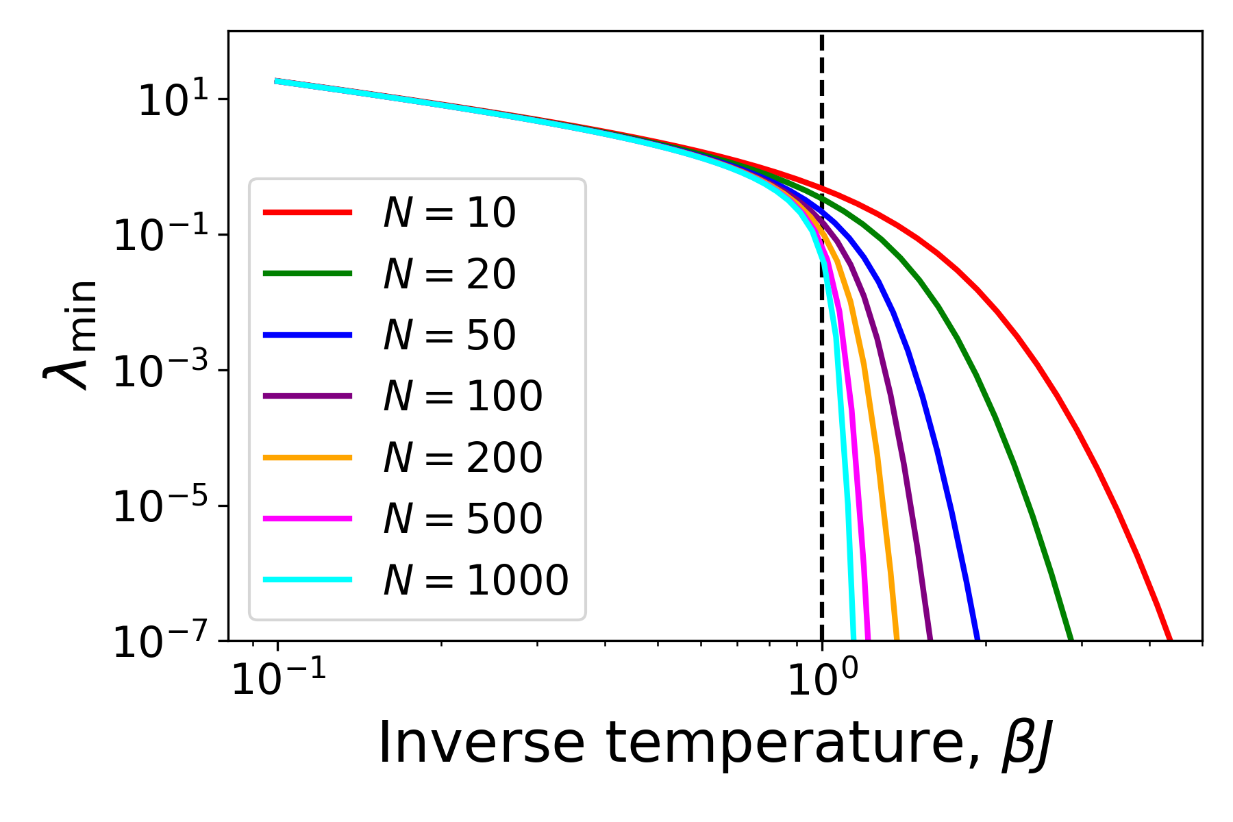
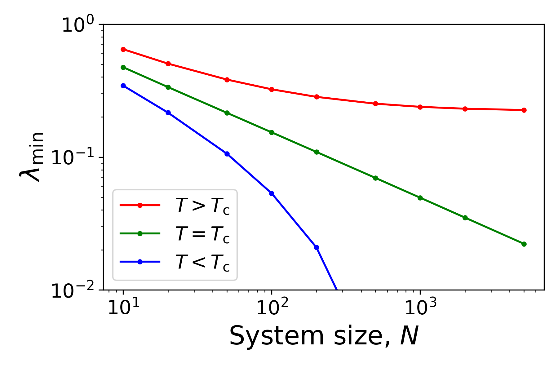
,
From the thermodinamic limit we can determine the dynamical critical exponent. Figure 4 shows as the function of the reduced temperature (). This follows an easy power law, because . In the next section we will see that this result can be obtained from the mean field approximation.
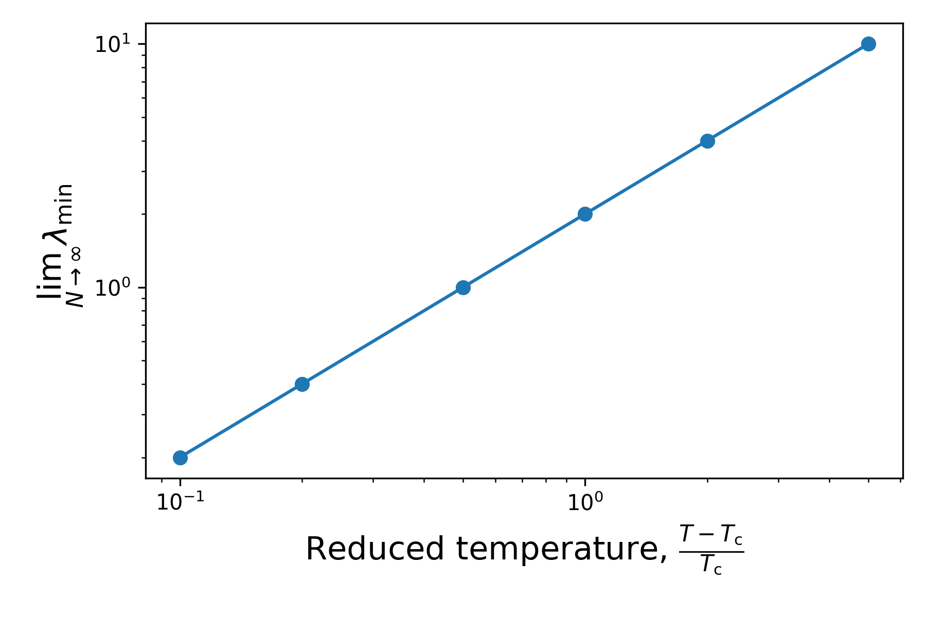
,
V Time dependent mean field equation
Since the primary interest is the magnetization (), we would like to derive a differential equation for it. Using the definition of and the master equation we get
| (29) |
The matrix component is nonzero if the Hamming distance between and is one. Introducing
| (30) |
we can rewrite the double sum in (29).
| (31) |
In the second step the identity was used. The nonzero elements of are the function of the energy difference:
| (32) |
where , so this is still the function of the random variable, but because it is not a function of . Since can be only or the as a function of must have the
| (33) |
form. Using (7) yields
| (34) |
then substituting back to (31) gives
| (35) |
Equation (35) is similar to the Callen equation Callen 1963; Parisi and Shankar 1988 , where the averaging is outside the hyperbolic function. In order to get a closed equation to the expected values the average must move inside, and instead of the random variables their expected values must be written.
| (36) |
The right-hand side contains the self-consistent equation from the equilibrium statistical physics, hence if the equation of state is satisfied, then .
Equation (36) contains both the real time and the temperature of the bath. The temperature can be also time dependent, and in that case what we could get is a thermal annealing, but if the temperature is constant we can determine the relaxation time, and the dynamical critical exponent. If , where is the equilibrium solution and is small, then the linearized equation of (36) is
| (37) |
where . Using the identity, and the equation of state we get to
| (38) |
Equation (38) contains the inverse susceptibility of the mean field Ising model.
| (39) |
where
| (40) |
Substituting the inverse susceptibility back into (38) yields
| (41) |
This is a well known equation in the theory of dynamical critical phenomena Hohenberg and Halperin 1977, but it is usually derived from the phenomenological equation. Now we can see, how it is related to a master equation and the spin-boson model. If the system is symmetric in a sense, that all the spins behave the same, then (41) simplifies to
| (42) |
where .
VI Time dependent mean field equation for the uniform Ising model
As before in section IV the uniform Ising model will be studied, because in the equilibrium case in the thermodynamic limit it gives back the exact results. According to (40) the mean field free energy is
| (43) |
and the time dependent mean field equation is
| (44) |
If the critical temperature is , and above this temperature the equilibrium solution is . The inverse susceptibility is
| (45) |
therefore
| (46) |
where in the Ohmic bath. Equation (46) is the same result that we have already seen in figure 4. As in the equilibrium statistical physics the mean field approximation gives back the exact result for the uniform model in the thermodynamic limit.
At the critical temperature the inverse susceptibility is zero, the linear term vanishes, and we need the higher order terms. Taylor expanding (44) at around up to third order gives.
| (47) |
which has the
| (48) |
solution for large s, which means there isn’t a characteristic time.
Below the critical temperature the linearized equation is good again, only the changes. On the other hand equation (44) can give different solution than the (28) master equation. If we want to compare these two equations the initial condition must be also the same which gives a restriction to the initial condition of (28). In the mean field approximation the probability is a product of the one particle probabilities:
| (49) |
which means the initial probability of (28) is
| (50) |
If , then the master equation must converge to the solution, but the time dependent mean field equation finds the global minimum of the free energy if initially . If is finite and is in the valley of the global minimum (point A in figure 5), than in the limit the solution of the master equation converges to the mean field solution (figure 6(a)).


, , , , Ohmic bath
On the other hand if initially is in the valley of the local minimum (point B in figure 5), then the solution of the mean field equation converges to this local minimum, but the solutions of the master equation are totally different. The probabilities converge to the equilibrium
| (51) |
distribution, so they tend to approach for large values in the limit, but as grows, so does the relaxation time. In the thermodynamic limit the relaxation time diverges as in figure 3(b). In the limit the solution of the master equation converges to the solution of the mean field equation and none of them will approach the global minimum, because the relaxation time will be infinit.
VII Conclusion
In this work we have presented a Glauber-type master equation for the spin-boson model. Starting from the Redfield equation the population decoupled even without the secular approximation. The most relevant dynamical properties are encoded in the eigenvalues of the transition matrix of the master equation. They are temperature dependent, and behave significantly different below, above and at the critical temperature as a function of the system size. In the case of the uniform, fully connected Ising model, in the thermodynamic limit, above the critical temperature the relaxation time follows a power law: .
We have derived a time dependent mean field equation, which is an effective equation of the master equation, containing only the expected values. As every mean field theory it works best if the number of neighbours is large, so the fully connected Ising model is the best candidate, and the numerical simulations show that in the limit the master equation gives back the same solutions as the mean field equation.
Acknowledgement
This work was supported by NKFIH within the Quantum Technology National Excellence Program (Project No. 2017-1.2.1-NKP-2017-00001) and within the Quantum Information National Laboratory of Hungary, by the ELTE Institutional Excellence Program (TKP2020-IKA-05) financed by the Hungarian Ministry of Human Capacities, and Innovation Office (NKFIH) through Grant No. K134437.
References
- Ising (1925) E. Ising, Zeitschrift für Physik A Hadrons and Nuclei 31 (1925), 10.1007/bf02980577.
- Onsager (1944) L. Onsager, Phys. Rev. 65, 117 (1944).
- Baxter (1982) R. Baxter, Exactly Solved Models in Statistical Mechanics (Academic Press, 1982).
- Sólyom (2007) J. Sólyom, Fundamentals of the Physics of Solids: Volume 1: Structure and Dynamics, Vol. 1 (Springer Science & Business Media, 2007).
- Mézard et al. (1987) M. Mézard, G. Parisi, and M. Virasoro, Spin glass theory and beyond: An Introduction to the Replica Method and Its Applications, Vol. 9 (World Scientific Publishing Company, 1987).
- Harris et al. (2018) R. Harris, Y. Sato, A. Berkley, M. Reis, F. Altomare, M. Amin, K. Boothby, P. Bunyk, C. Deng, C. Enderud, et al., Science 361, 162 (2018).
- Farhi et al. (2000) E. Farhi, J. Goldstone, S. Gutmann, and M. Sipser, arXiv preprint quant-ph/0001106 (2000).
- Roland and Cerf (2002) J. Roland and N. J. Cerf, Physical Review A 65, 042308 (2002).
- Breuer et al. (2002) H.-P. Breuer, F. Petruccione, et al., The theory of open quantum systems (Oxford University Press on Demand, 2002).
- Schaller (2014) G. Schaller, Open quantum systems far from equilibrium, Vol. 881 (Springer, 2014).
- Redfield (1965) A. Redfield, in Advances in Magnetic and Optical Resonance, Vol. 1 (Elsevier, 1965) pp. 1–32.
- Lindblad (1976) G. Lindblad, Communications in Mathematical Physics 48, 119 (1976).
- Rebentrost et al. (2009) P. Rebentrost, M. Mohseni, I. Kassal, S. Lloyd, and A. Aspuru-Guzik, New Journal of Physics 11, 033003 (2009).
- Guerreschi et al. (2012) G. G. Guerreschi, J. Cai, S. Popescu, and H. J. Briegel, New Journal of Physics 14, 053043 (2012).
- Sieberer et al. (2016) L. M. Sieberer, M. Buchhold, and S. Diehl, Reports on Progress in Physics 79, 096001 (2016).
- Oppenheim et al. (1977) I. Oppenheim, K. E. Shuler, G. H. Weiss, et al., Stochastic processes in chemical physics (Mit Press, 1977).
- Vacchini and Breuer (2010) B. Vacchini and H.-P. Breuer, Physical Review A 81, 042103 (2010).
- Davies (1976) E. B. Davies, Quantum theory of open systems (Academic Press London, 1976).
- Leggett et al. (1987) A. J. Leggett, S. Chakravarty, A. T. Dorsey, M. P. Fisher, A. Garg, and W. Zwerger, Reviews of Modern Physics 59, 1 (1987).
- Albash and Lidar (2015) T. Albash and D. A. Lidar, Physical Review A 91, 062320 (2015).
- Takada and Nishimori (2016) K. Takada and H. Nishimori, Journal of Physics A: Mathematical and Theoretical 49, 435001 (2016).
- Cugliandolo et al. (2002) L. F. Cugliandolo, D. Grempel, G. Lozano, H. Lozza, and C. da Silva Santos, Physical Review B 66, 014444 (2002).
- Sinha and Dattagupta (2013) S. Sinha and S. Dattagupta, The European Physical Journal B 86, 96 (2013).
- Suárez et al. (1992) A. Suárez, R. Silbey, and I. Oppenheim, The Journal of chemical physics 97, 5101 (1992).
- Gaspard and Nagaoka (1999) P. Gaspard and M. Nagaoka, The Journal of chemical physics 111, 5668 (1999).
- Nakajima (1958) S. Nakajima, Progress of Theoretical Physics 20, 948 (1958).
- Zwanzig (1960) R. Zwanzig, The Journal of Chemical Physics 33, 1338 (1960).
- Wang et al. (2015) C. Wang, J. Ren, and J. Cao, Scientific reports 5, 11787 (2015).
- Wauters et al. (2017) M. M. Wauters, R. Fazio, H. Nishimori, and G. E. Santoro, Physical Review A 96, 022326 (2017).
- Callen (1963) H. B. Callen, Phys. Letters 4 (1963).
- Parisi and Shankar (1988) G. Parisi and R. Shankar, Physics Today 41, 110 (1988).
- Hohenberg and Halperin (1977) P. C. Hohenberg and B. I. Halperin, Reviews of Modern Physics 49, 435 (1977).