Improved Approximation of Dispatchable Region in Radial Distribution Networks via Dual SOCP
Abstract
The concept of dispatchable region is useful in quantifying how much renewable generation power the system can handle. In this paper, we aim to provide an improved dispatchable region approximation method in distribution networks. First, based on the nonlinear Dist-Flow model, an optimization problem that minimizes the sum of slack variables is formulated to describe the dispatchable region. The nonconvexity caused by alternating-current (AC) power flow constraints makes it intractable. To deal with this issue, the problem is relaxed to a second-order cone program (SOCP) whose strong dual problem is derived. Then, an SOCP-based projection algorithm is developed to construct a convex polytopic approximation. We prove that the proposed algorithm can generate the accurate SOCP-relaxed dispatchable region under certain conditions. Furthermore, a heuristic method is proposed to approximately remove the regions that make the SOCP relaxation inexact. The final region obtained is the difference of several convex sets and can be nonconvex. Thus, the proposed approach may provide a better approximation of the actually nonconvex dispatchable region than previous work that could construct convex sets only. Numerical results demonstrate that the proposed method can achieve a high accuracy of approximation with simple computation.
Index Terms:
AC power flow, distribution networks, dispatchable region, optimization, second-order cone programNomenclature
-A Constant parameters
-
Resistance and reactance of line .
-
Controllable active power limit at node .
-
Controllable reactive power limit at node .
-
Voltage safety limit at node .
-
Current safety limit on line .
-
Constant matrices in the feasibility problem.
-
Constant vectors in the feasibility problem.
-
Constant matrices and vectors in SOCP.
-
Bounds for the initial polytope in Algorithm 1.
-
Positive parameters used in Algorithm 2.
-B Variables
-
Controllable power injection at node .
-
Renewable active power generation at node .
-
Squared voltage magnitude at node .
-
Squared current magnitude on line .
-
Active and reactive power flows onto line .
-
Vector of state variables .
- , ,
-
Vectors of nonnegative slack variables.
-
Auxiliary variables in SOCP for line .
-
Dual variables for equality constraints.
-
Dual variables for inequality constraints.
-C Optimization problems, values, sets
-
Feasibility problem for renewable generation .
-
Minimum objective value of .
-
Dispatchable region of , in which .
-
SOCP relaxation of .
-
Minimum objective value of .
-
SOCP-relaxed dispatchable region of .
-
Dual problem of , also an SOCP.
-
Dual objective function.
-
Maximum objective value of .
-
Dual SOCP with feasible set tightened by .
-
Maximum objective value of .
-
Polytopic approximation of , by Algorithm 1.
-
SOCP-inexact region of .
-
Approximation of using dual SOCP.
-
Polytopic approximation of , by Algorithm 2.
I Introduction
With the benefits of near-zero carbon emissions and low operating costs, distributed renewable power is experiencing tremendous expansion in recent years [1]. Meanwhile, its volatile and intermittent features pose great challenges to electric grid operation, especially the distribution system. Unlike the bulk system, distribution system has few controllable units and a stronger coupling of active and reactive power flows due to its high resistance to reactance ratio [2]. This makes it even harder to accommodate the fluctuating renewable generations. Therefore, characterizing the renewable power capacities that can be safely hosted by a distribution network prior to its actual operation is vital. This necessitates finding all renewable power outputs that can ensure solvability of the power flow equations and satisfaction of safety limits.
The first requirement is solvability of the power flow equations. For a transmission network modeled by direct-current (DC) power flow, solvability is easy to check since a closed-form solution can be obtained [3]. However, for distribution networks, the lossless DC model is not accurate enough since the distribution lines have higher resistance to reactance ratios. Some literature proved sufficient conditions under which the alternating current (AC) power flow equations are solvable, by utilizing Banach fixed-point theorem for contraction mappings [4, 5] or Brouwer fixed-point theorem for continuous mappings over compact convex sets [6, 7]. Nonetheless, those methods cannot be readily applied to output the dispatchable region since they are based on power flow equations and can hardly deal with inequality safety constraints.
To further take into account the second requirement, i.e., satisfaction of safety limits, optimization based methods were developed. Two well-known concepts are the do-not-exceed limit (DNEL) [8] and the dispatchable region [9]. The DNEL provides an allowable power interval for each renewable generator based on robust optimization. Data-driven approach [10] and topology control [11] were incorporated to improve the accuracy of DNEL. The correlation between different renewable generators is ignored in DNEL, so the obtained capacity regions can be conservative. The dispatchable region further considers those correlations and provides the exact region consisting of all renewable power outputs that can be accommodated. An adaptive constraint generation algorithm was proposed to generate the dispatchable region [12]. The interaction between different prosumers with renewable generators was considered in [13]. Similarly, dispatchable region can be applied to quantify the allowable variation of loads based on Fourier–Motzkin elimination [14]. The above studies are based on DC power flow models.
As mentioned above, AC power flow model is a must for a distribution network. Reference [15] solved nonlinear programs to get a set of boundary points that each make a different safety limit binding, and then built a dispatchable region heuristically as the convex hull of those boundary points. Linearized models were used to approximate the real dispatchable region under AC power flow [16, 17]. However, there is no guarantee that all scenarios inside the obtained region are feasible. Reference [2] used the intersection of the dispatchable regions generated from two linearized models to output a more accurate approximation. To guarantee feasibility, certified inner approximations of dispatchable regions were solved from convex programs based on a tightened-relaxed second-order cone approximation [18] or refined linear approximations [19, 20] to AC power flow. However, such estimation typically only works for a specific objective function that merely explores the dispatchable region towards a single direction or with a specific shape of the renewable generation vector. Moreover, all the aforementioned regions are convex, while the actual dispatchable region can be nonconvex due to the AC power flow constraints.
In this paper, we propose an alternative method to complement the literature above. Our main contributions are two-fold:
- 1)
Accurate Dispatchable Region of the Second-Order Cone (SOC) Relaxed Model. A nonlinear Dist-Flow model based optimization problem is developed to characterize the dispatchable region, which is hard to solve due to its nonconvexity. Therefore, we first relax the problem to a convex second-order cone program (SOCP). Then, unlike reference [2] that further linearized the SOC constraint using polyhedral approximation [21], we generate the dispatchable region directly without further linearization. To be specific, the dual problem of the SOCP is derived and strong duality holds as proven in Proposition 1. We then propose a projection algorithm (Algorithm 1) to construct a polytopic approximation of the SOCP-relaxed dispatchable region. We prove that the approximation is accurate under certain conditions.
- 2)
Removal of SOCP-Inexact Regions. The other inaccuracy lies in the possible inexactness of the SOC relaxation. In fact, the actual dispatchable region may be nonconvex, but the algorithms developed in previous studies can only generate convex regions. Distinctly, we propose a heuristic method to find out the SOCP-inexact regions by requiring the corresponding dual variables to be larger than some small positive values. Removing the SOCP-inexact regions from the region generated by Algorithm 1 from the SOC relaxed model, we can build a tighter approximation of the actual dispatchable region. The proposed method provides an innovative idea for constructing an accurate dispatchable region as the difference of several convex sets. Numerical results show that the proposed method can approximate the complicated dispatchable region with a simple polytope after moderate computation, while preserving relatively good accuracy. It can also reach a satisfactory balance between ensuring safety and reducing conservatism.
The rest of this paper is organized as follows. Section II introduces the power network model we use. Section III defines the dispatchable region and the optimization problem to characterize it. Section IV elaborates our method to approximate the dispatchable region. Section V reports numerical experiments, and Section VI concludes the paper.
II Power network model
Consider the single-phase equivalent model of a distribution network, which is a radial graph with a set of nodes and a set of lines. Index the nodes as , where represents the root node (slack bus). For convenience, we treat the lines as directed; for example, if a line connects nodes , where node is closer to the root than node , then the line directs from to and is denoted by . The power flow in the network at a particular time instant can be modeled by the classic Dist-Flow equations purely in real numbers [22, 23], elaborated as follows.
At each node : let denote the squared voltage magnitude; aggregate all the controllable power sources and loads into a complex power injection ; denote the uncontrollable active power generation of a renewable energy source as . Let denote the squared current magnitude through each line . Let and denote the net active and net reactive power, respectively, that are sent by node onto line ; they are different from the net power arriving at node due to power loss, and are negative if node receives power from line . Let , denote the constant resistance and reactance of line , respectively. The Dist-Flow equations are:
| 0 | (1a) | |||||
| 0 | (1b) | |||||
| 0 | (1c) | |||||
| 0. | (1d) | |||||
Suppose renewable energy sources only exist at a subset of nodes , whose cardinality is . For nodes , set constant . The variables in Dist-Flow equations (1) are grouped as follows:
- •
Renewable power generation , which is treated as input to the system;
- •
State variables , where each of , , , , , is a column vector indexed by .
Remark: Without loss of generality, we assume there is only one node, indexed as node , connected to the root node . In this case, the power exchange between the distribution network and the upper grid at node is , so that it is just considered as part of , not . As customary, assume is a given constant and thus not in state variable . The radial network has lines, where each line can be uniquely indexed by its destination node , so that we can index line variables , , by .
Assume known capacity limits of controllable power:
| (2a) | |||||
| (2b) | |||||
At any node where there are only fixed (or zero) power injections, the constant limits can be set as () and/or (). In addition, power system operations require the following safety limits to be satisfied:
| (3a) | |||||
| (3b) | |||||
where the voltage limits , for all nodes and the current limits for all lines are given as positive constants.
With the model above, we next define and analyze the dispatchable region of renewable power generation.
III Dispatchable region and relaxation
In this paper, the dispatchable region is the region of renewable power generation , for which there is a feasible dispatch. Its formal definition is provided below.
Definition 1.
For conciseness, we rewrite the linear part (1a)–(1c) of Dist-Flow equations as and affine inequalities (2)–(3) as , where both equality and inequality are element-wise, and constant matrices and vectors , , , , are provided in Appendix-A. Given any , we introduce the following optimization to check its feasibility.
| (4a) | |||||
| over | |||||
| s. t. | (4b) | ||||
| (4c) | |||||
| (4d) | |||||
| (4e) | |||||
where in objective (4a) is a row vector of all ones. Any element of the slack variable can increase as needed to satisfy the corresponding inequality constraint, but only can guarantee feasibility in terms of (1)–(3). Therefore, denoting the minimum objective value of as , the dispatchable region in Definition 1 is equivalently:
Due to the nonconvex quadratic inequality constraint (4e), problem is nonconvex and thus hard to analyze. By removing (4e) and rewriting (4d), we relax to a convex second order cone program (SOCP):
| (5a) | |||||
| over | |||||
| s. t. | (4b)–(4c) | (5b) | |||
| (5c) | |||||
where , , and vertically stack , , and respectively for all lines . Row vector and scalar number are also stacked vertically for all as and . The constant matrices and vectors , , , are provided in Appendix-B, which make:
and thus make (5b)–(5c) equivalent to (4d).11 1 Given , the values of in (4d) and (5c) are generally not equal, but we do not differentiate notation due to their identical role as slack variables.
Problem facilitates the definition of an SOCP-relaxed dispatchable region:
where is the minimum objective value of . It is obvious that , i.e., is a relaxation of .
A common practice to further simplify the dispatchable-region characterization is to outer approximate the second-order cone (5c) with a polytopic cone, which can achieve arbitrary precision by constructing sufficiently many planes tangent to the surface of the second-order cone [21, 24]. Consequently, is relaxed to a linear program, and then the algorithm in [9, 12, 13] can be employed to get a convex polytopic outer approximation of . In this work, we propose an alternative method that does not rely on such linearization. Instead, we work directly on the SOCP and its dual problem to preserve the intrinsic nonlinearity of the AC power flow model and hence the accuracy of our characterization.
IV Polytopic approximation algorithms
To offer a closed-form approximation of dispatchable region , we first develop a convex polytopic approximation of its relaxation via the dual problem of SOCP . We then develop a heuristic method to approximately remove the renewable generations that make the SOCP relaxation inexact, resulting in a tighter approximation of .
IV-A Dual SOCP
Let denote the dual variables for the equality constraints in problem , with for (4b) and for (5b) vertically stacking . Let denote the dual variables for the inequality constraints, with for (4c) and for (5c). Then the Lagrangian of is:
| (6) | |||||
Through we can get the dual objective function. By (6), can only attain a finite minimum over when the dual variables satisfy:
| (7a) | |||||
| (7b) | |||||
| (7c) | |||||
Note that in (7a) is a general requirement for all the dual variables associated with inequality constraints, and (7c) must hold by noticing
When (7) is satisfied, all the terms containing in (6) attain their minimum value zero, and hence we obtain the dual problem for , which is also an SOCP:
| s. t. | (7). |
Let denote the objective function and denote the maximum objective value of . The following result lays the foundation for approximating the SOCP-relaxed dispatchable region via the dual SOCP .
Proposition 1.
For all , strong duality holds between and , i.e., their optimal values .
Proof:
Consider an arbitrary . Since problem is convex, it is sufficient to prove Slater’s condition [25, Section 5.2.3], i.e., existence of that satisfies affine constraints (4b)(4c)(5b) and strictly satisfies (5c).
Indeed, it is adequate to find a point to satisfy (4b), i.e., (1a)–(1c); then one can explicitly determine by (5b) and always find large enough to make (4c)(5c) (strictly) feasible, satisfying Slater’s condition. Such a point can be easily found as follows: set ; determine backward from the leaves to the root of the radial network, using (1a)–(1b); then determine forward from the root to the leaves, using (1c). This completes the proof. ∎
By Proposition 1, the relaxed region is equivalently:
| (8) | |||||
where the second equality holds because can always be attained at the dual feasible point .
Proposition 2.
is a convex set.
Proof:
Consider arbitrary and . Denote . Then for every satisfying (7), we have:
where the first equality is due to linearity of with respect to when is fixed, and the inequality holds because . Therefore . By the definition of a convex set, is convex. ∎
IV-B Approximating SOCP-relaxed dispatchable region
We propose Algorithm 1 to approximate defined in (8). It starts with a region that is large enough to contain . Then it solves the dual SOCP for every vertex of polytope , records the vertex that most severely violates the condition in (8), and adds a corresponding cutting plane to remove that vertex from . Meanwhile, all the vertices that satisfy the condition in (8) are added to and never checked again.
Proposition 3.
The output in an arbitrary iteration of Algorithm 1 is an outer approximation of .
Proof:
Note the initial contains . We next prove that any cutting plane added to would not remove any point in . To show that, consider an arbitrary removed by a cutting plan whose coefficients are . Then there must be . Since is dual feasible satisfying (7), we have by (8). ∎
Unlike [9, 13] that based on linear programs, the SOCP-relaxed dispatchable region may not be the intersection of a finite number of cutting planes (i.e., a convex polytope). Therefore, Algorithm 1 may not guarantee for all vertices in a finite number of iterations. However, if it does so, as what always happens in our numerical experiments, it will produce a nice result as follows.
Proposition 4.
If Algorithm 1 terminates with in a finite number of iterations, it returns the accurate SOCP-relaxed dispatchable region, i.e., .
Proof:
Proposition 3 has shown . If Algorithm 1 terminates with after adding a finite number of cutting planes, then it returns a convex polytope . Moreover, all the vertices satisfy , therefore, by (8). This fact, together with the convexity of shown in Proposition 2, implies . Thus we have proved . ∎
An immediate corollary of Proposition 4 is that if is not a polytope, then Algorithm 1 cannot terminate in a finite number of iterations with . If that happens, one can terminate Algorithm 1 when reaching the maximum number of iterations , to obtain a convex polytopic outer approximation of . In this sense, the outcome of Algorithm 1 serves as a posterior indicator of the structure of .
IV-C Removing SOCP-inexact renewable generations
Remember our goal is to characterize the dispatchable region , whereas studied so far is just a SOCP-relaxation of . To overcome this drawback, we design a heuristic to approximately remove the SOCP-inexact region from . The renewable generations are feasible in terms of the SOCP relaxation but infeasible in terms of , as formally defined below.
Definition 2.
A vector of renewable power generation is SOCP-inexact, if every optimal solution of satisfies:
The SOCP-inexact region of is defined as:
Our next focus is to build an approximation of . For that, we consider the following set defined on the dual SOCP:
By complementary slackness [25, Section 5.5.2], for every primal-dual optimal of and , there is:
This implies . Although may not hold, their difference can only occur under rare circumstances where at a primal-dual optimal. Hence we focus on as an approximation of .
Given an arbitrary , the maximum objective value of is but with some so the SOC relaxation is inexact (except for some very rare case). To approximate , first we add the following constraint to tighten the dual feasible set (7):
| (9) |
where the inequality is element-wise and is a vector of all strictly positive parameters, whose design will be elaborated later. Consider the tightened dual SOCP:
| s. t. | (7), (9) |
and let denote its maximum objective value. For , there must be , because otherwise would have an optimal solution that satisfies (9), contradicting the definition of . Actually for some that depends on and .
The idea above inspires us to approximate (or ) by
To this end, Algorithm 2 can be designed using a similar procedure to Algorithm 1. Algorithm 2 returns a convex polytope that guarantees for all , which is an approximation of (or ). Removing from , we can obtain an approximation of the actual dispatchable region . To make Algorithm 2 more robust, we may choose for the added cutting plane in each iteration.
Remark: The parameters and are essential for Algorithm 2. A general guideline is that (1) given , choosing a smaller and (2) given , choosing a bigger will both make bigger and lead to a smaller (more conservative) approximation of . Moreover, sometime it is difficult for Algorithm 2 to use a single convex polytope to accurately approximate the most likely nonconvex . To deal with this difficulty, we propose to run Algorithm 2 multiple times with different vectors . As a result, we obtain multiple convex polytopes whose union serves as a better approximation of . Those vectors can be selected in the following way. We traverse the vertices of , select one vertex , and solve the dual SOCP to get an optimal solution . Then is constructed by keeping all the strictly positive elements of as they are, and add a small positive perturbation to all the zero elements.
| SOCP-relaxed Region | = | SOCP-exact Region | + | SOCP-inexact Region | |
|---|---|---|---|---|---|
| Actual | = | + | |||
| Approx. | = | + | |||
| Method | Algorithm 1 | Algorithm 2 |
Summary. The relationship of different regions mentioned in this paper is summarized in TABLE I. As discussed, the dispatchable region , where is the SOCP-relaxed dispatchable region and is the SOCP-inexact region. We develop Algorithm 1 to get , a convex polytopic approximation of ; and Algorithm 2 to get , a convex polytopic approximation of . Algorithm 2 can run multiple times to obtain a more accurate approximation of nonconvex (or ). The outputs of multiple runs of Algorithm 2 are then removed from to obtain a generally nonconvex polytopic approximation of .
V Case Studies

In this section, we conduct numerical experiments on the IEEE 33-bus system whose topology is in Fig. 1. The proposed algorithms are implemented to approximate the dispatchable region of renewable generation at nodes 13 and 29, respectively. Then, we test the impact of several factors and compare with other approaches.
V-A Benchmark
| Generator | Location | (p.u.) | (p.u.) |
|---|---|---|---|
| G1 | node 10 | 0.4 | 0.6 |
| G2 | node 18 | 0.3 | 0.4 |
| G3 | node 23 | 0.4 | 0.6 |
| G4 | node 25 | 0.3 | 0.5 |
| G5 | node 33 | 0.4 | 0.6 |

In the IEEE-33 bus system, there are 5 controllable generators whose parameters are given in TABLE II. Two renewable generators are connected to nodes 13 and 29, respectively. For comparison, the actual SOCP-relaxed region and the actual dispatchable region without relaxation are generated as in Fig. 2. This can be done by checking the feasiblity of a nonlinear optimization with (1)-(3) as its constraints, over sample points in the space using the nonlinear solver IPOPT. As we can see from Fig. 2, the actual dispatchable region can be nonconvex and the SOCP-relaxed region is not accurate enough. In the following, we apply the proposed algorithms to output a more accurate region.
First, we test the performance of Algorithm 1. We observe that algorithm terminates with in 25 iterations, taking about 289.84s. The output regions in the 2nd, 5th, 10th, and final iterations are given in Fig. 3. The Algorithm 1 removes the nondispatchable regions iteratively (the blue region is becoming smaller), and finally returns a convex polytope exactly the same as the actual SOCP-relaxed region (dashed line). This validates Proposition 4.
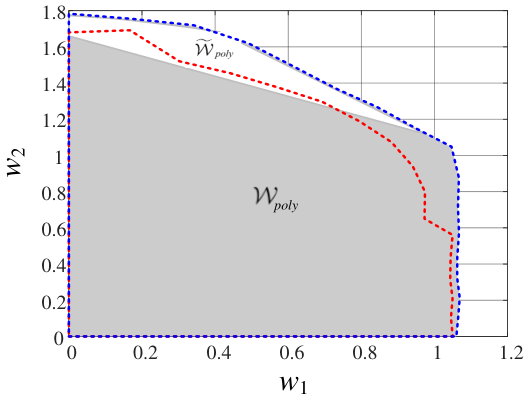
Even though Algorithm 1 can output the accurate SOCP-relaxed dispatchable region, as we can see in Fig. 2, there is still a gap between the actual dispatchable region and the relaxed one . If the renewable generator output lies in the gap area, there is actually no feasible dispatch that satisfies power flow equation (1) and safety limits (2)-(3). Thus, using the SOCP-relaxed region as a guidance will threaten power system security. In this paper, Algorithm 2 is developed to further remove the nondispatchable points. As in Fig. 4, the (white area) generated by Algorithm 2 is removed and the resulting region (grey area) is closer to the actual region (red dash line). This shows the great potential of the proposed algorithm in improving the accuracy of dispatchable region in a distribution system. The operational risk under the obtained region and the SOCP-relaxed region will be compared later in TABLE IV.
V-B Impact of different factors
In the following, we test the impact of two factors (adjustable capability of controllable generators and current limit ) on the shape of the dispatchable region and the performance of the proposed algorithm.
| Generator | Case L | Case H | ||
|---|---|---|---|---|
| No. | (p.u.) | (p.u.) | (p.u.) | (p.u.) |
| G1 | 0.4 | 0.5 | 0 | 0.6 |
| G2 | 0.3 | 0.4 | 0 | 0.4 |
| G3 | 0.4 | 0.5 | 0 | 0.6 |
| G4 | 0.4 | 0.5 | 0 | 0.5 |
| G5 | 0.4 | 0.5 | 0 | 0.6 |

To show how influences the dispatchable region, we test three cases: (1) Benchmark, which has the same setting as in Section V-A. (2) Case L, where the generators have less adjustable capability than the benchmark. (3) Case H, where the generators have more adjustable capability than the benchmark. The parameters of the Cases L and H are given in TABLE III. The regions returned by Algorithm 1 () and Algorithm 2 () are given in Fig. 5. Subfigures (a), (b) are for Case L and subfigures (c), (d) are for Case H. The changes of under three cases are recorded in Fig. 6.
As shown in Figs. 3 and 5, Algorithm 1 can always output the accurate SOCP-relaxed dispatchable region, i.e., . The final dispatchable regions (grey area) returned by the proposed algorithms are much closer to the actual ones compared with the SOCP-relaxed regions. In addition, as the adjustable capability of generators decreases, the system’s ability to accommodate volatile renewable power becomes weaker, and thus, the dispatchable region becomes smaller. We also find that with a weaker adjustable capability, the actual dispatchable region is more likely to be nonconvex and to differ more from the SOCP-relaxed region. The difference between the red dash line and the blue dash line in Fig. 5(b) is more significant than that in Fig. 5(d). In the future power systems, more renewable generators are replacing the controllable generators, so the use of an SOCP-relaxed dispatchable region is not accurate enough. Therefore, the proposed Algorithms 1-2 to remove the nondispatchable points will be helpful.
| FR() | FR() | Reduction | Time(s) | |
|---|---|---|---|---|
| Benchmark | 10.4% | 4.5% | 56.73% | 289.84 |
| Case L | 15.7% | 8.7% | 44.59% | 291.01 |
| Case H | 3.5% | 2.5% | 28.57% | 724.60 |
In Fig. 6, the under all three cases decrease towards zero when Algorithm 1 terminates. The computational times are 289.84s (Benchmark), 291.01s (Case L), and 724.60s (Case H), respectively, showing that our algorithm is efficient. Moreover, we randomly generate 2000 points in the SOCP-relaxed dispatchable region and the final obtained region , and calculate the failure rate defined as
| (10) |
The failure rates under three cases are summarized in TABLE IV. In all three cases, the proposed method can greatly reduce the failure rate, and the reduction is more than 50% under benchmark. This can help better ensure system security. Moreover, we can find that in a system with relatively small adjustable capability, the reduction is more significant.
Furthermore, we test the impact of current limit by running two other cases where we halve and double the , respectively. The obtained region are shown in Fig. 7. The computation times are both less than 500s, which is acceptable. A more stringent line-flow limit results in a smaller dispatchable region and also a greater deviation between the relaxation region and the exact region .

V-C Comparison with other methods
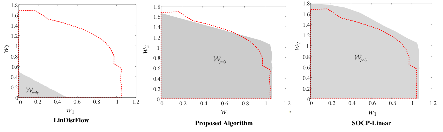
We then compare the performance of the proposed algorithms with two well-known approaches based on (1) Linearized DistFlow model [22] (denoted as LinDistFlow); (2) Polyhedral approximation of the SOCP-relaxed model [24] (denoted as SOCP-Linear). These two models are linear programs so that the adaptive constraint generation algorithm in [12] can be applied to generate the region. The results are shown in Fig. 8. Theoretically, the LinDistFlow region can be an inner/outer approximation or a region that intersects the actual dispatchable region. In the benchmark case, the LinDistFlow region is very small and conservative. The SOCP-Linear region is always an outer approximation of the actual region. We can see that it is very close to the SOCP-relaxed region . To better illustrate the results under three approaches, we calculate the failure rate (10) and the missing rate (MR) defined below.
| (11) |
The failure rate and missing rate under three approaches are compared in TABLE V. We can find that, in this simulation case, the LinDistFlow region is an inner approximation so its failure rate is zero. However, it has a very high missing rate, meaning that the region is too conservative. The SOCP-Linear region is always an outer approximation so its missing rate is zero, but its failure rate is high. The proposed method can achieve a good balance between ensuring security and reducing conservatism.
| FR() | MR() | |
|---|---|---|
| LinDistFlow | 0% | 91.1% |
| Proposed Method | 4.5% | 2.7% |
| SOCP-Linear | 11.8% | 0% |
VI Conclusion
In this paper, we develop an improved approximation of the renewable generation dispatchable region in radial distribution networks. First, a nonconvex optimization problem is formulated to describe the dispatchable region. The nonconvex problem is then relaxed to a convex SOCP. An SOCP-based projection algorithm (Algorithm 1) is proposed to generate the accurate SOCP-relaxed dispatchable region under certain conditions. In addition, a heuristic method (Algorithm 2) is developed to remove the SOCP-inexact region from the region obtained above. Therefore, the final region can better approximate the actual nonconvex dispatchable region. Our main findings are:
- •
The proposed method can reduce the operational risk (quantified by failure rate) by more than 50% compared with the SOCP-relaxed region.
- •
The proposed method has a greater potential in the future power system with fewer controllable units and thus weaker adjustable capability.
- •
Compared with existing approaches (LinDistFlow and SOCP-Linear), the proposed method achieves a better tradeoff between security and conservatism.
This paper provides an innovative perspective for constructing the dispatchable region: While the existing literature can only generate convex regions, the proposed algorithm can generate nonconvex approximations. For future work, we aim to improve the accuracy of the proposed algorithms by properly setting the initial points for heuristic searching.
Appendix. Constant parameters
This appendix provides in full detail the constant matrices, vectors, and numbers used in Section IV.
VI-A Equation (4): , , , ,
The vector is arranged in the order explained in Section II. Let be the incidence matrix of the radial network, with its element at the -th row, -th column:
Removing the first row of , we get the reduced incidence matrix . Define diagonal matrices and . Denote the all-zero matrix as , identity matrix as , and -dimensional all-zero column vector as . We have:
Moreover, we define:
and let be a submatrix of that contains only the columns corresponding to the nodes with nonzero renewable generation . Define column vectors , , similarly , , , , and . To write inequalities (2)(3) as , we need:
VI-B Equation (5): , , ,
To make (5b)–(5c) the same as:
we need , , , as follows:
- •
For all , is sparse matrix with all elements zero except its element at the first row, -th column equal to ; at the second row, -th column equal to 2; at the third row, -th column equal to (if ), and -th column equal to .
- •
For all except , is a three-dimensional column vector of all zeros; .
- •
For all , is a -dimensional row vector of all zeros except its -th (if ) and -th elements both equal to .
- •
for all except ; .
References
- [1] J. Ahmad, M. Tahir, and S. K. Mazumder, “Dynamic economic dispatch and transient control of distributed generators in a microgrid,” IEEE Systems Journal, vol. 13, no. 1, pp. 802–812, 2018.
- [2] Z. Shen, W. Wei, T. Ding, Z. Li, and S. Mei, “Admissible region of renewable generation ensuring power flow solvability in distribution networks,” IEEE Systems Journal, 2022.
- [3] A. Soroudi, A. Rabiee, and A. Keane, “Stochastic real-time scheduling of wind-thermal generation units in an electric utility,” IEEE Systems Journal, vol. 11, no. 3, pp. 1622–1631, 2015.
- [4] S. Bolognani and S. Zampieri, “On the existence and linear approximation of the power flow solution in power distribution networks,” IEEE Transactions on Power Systems, vol. 31, no. 1, pp. 163–172, 2015.
- [5] C. Wang, A. Bernstein, J.-Y. Le Boudec, and M. Paolone, “Explicit conditions on existence and uniqueness of load-flow solutions in distribution networks,” IEEE Transactions on Smart Grid, vol. 9, no. 2, pp. 953–962, 2016.
- [6] K. Dvijotham, H. Nguyen, and K. Turitsyn, “Solvability regions of affinely parameterized quadratic equations,” IEEE Control Systems Letters, vol. 2, no. 1, pp. 25–30, 2017.
- [7] J. W. Simpson-Porco, “A theory of solvability for lossless power flow equations—part II: Conditions for radial networks,” IEEE Transactions on Control of Network Systems, vol. 5, no. 3, pp. 1373–1385, 2017.
- [8] J. Zhao, T. Zheng, and E. Litvinov, “Variable resource dispatch through do-not-exceed limit,” IEEE Transactions on Power Systems, vol. 30, no. 2, pp. 820–828, 2015.
- [9] W. Wei, F. Liu, and S. Mei, “Dispatchable region of the variable wind generation,” IEEE Transactions on Power Systems, vol. 30, no. 5, pp. 2755–2765, 2015.
- [10] F. Qiu, Z. Li, and J. Wang, “A data-driven approach to improve wind dispatchability,” IEEE Transactions on Power Systems, vol. 32, no. 1, pp. 421–429, 2016.
- [11] A. S. Korad and K. W. Hedman, “Enhancement of do-not-exceed limits with robust corrective topology control,” IEEE Transactions on Power Systems, vol. 31, no. 3, pp. 1889–1899, 2015.
- [12] W. Wei, F. Liu, and S. Mei, “Real-time dispatchability of bulk power systems with volatile renewable generations,” IEEE Transactions on Sustainable Energy, vol. 6, no. 3, pp. 738–747, 2015.
- [13] Y. Chen, W. Wei, H. Wang, Q. Zhou, and J. P. Catalão, “An energy sharing mechanism achieving the same flexibility as centralized dispatch,” IEEE Transactions on Smart Grid, vol. 12, no. 4, pp. 3379–3389, 2021.
- [14] A. Abiri-Jahromi and F. Bouffard, “On the loadability sets of power systems—part II: Minimal representations,” IEEE Transactions on Power Systems, vol. 32, no. 1, pp. 146–156, 2016.
- [15] S. Chen, Z. Wei, G. Sun, W. Wei, and D. Wang, “Convex hull based robust security region for electricity-gas integrated energy systems,” IEEE Transactions on Power Systems, vol. 34, no. 3, pp. 1740–1748, 2018.
- [16] C. Wan, J. Lin, W. Guo, and Y. Song, “Maximum uncertainty boundary of volatile distributed generation in active distribution network,” IEEE Transactions on Smart Grid, vol. 9, no. 4, pp. 2930–2942, 2016.
- [17] Y. Liu, Z. Li, Q. Wu, and H. Zhang, “Real-time dispatchable region of renewable generation constrained by reactive power and voltage profiles in AC power networks,” CSEE Journal of Power and Energy Systems, vol. 6, no. 3, pp. 528–536, 2019.
- [18] M. Nick, R. Cherkaoui, J.-Y. Le Boudec, and M. Paolone, “An exact convex formulation of the optimal power flow in radial distribution networks including transverse components,” IEEE Transactions on Automatic Control, vol. 63, no. 3, pp. 682–697, 2017.
- [19] H. D. Nguyen, K. Dvijotham, and K. Turitsyn, “Constructing convex inner approximations of steady-state security regions,” IEEE Transactions on Power Systems, vol. 34, no. 1, pp. 257–267, 2018.
- [20] N. Nazir and M. Almassalkhi, “Convex inner approximation of the feeder hosting capacity limits on dispatchable demand,” in IEEE Conference on Decision and Control, 2019, pp. 4858–4864.
- [21] A. Ben-Tal and A. Nemirovski, “On polyhedral approximations of the second-order cone,” Mathematics of Operations Research, vol. 26, no. 2, pp. 193–205, 2001.
- [22] M. E. Baran and F. F. Wu, “Optimal capacitor placement on radial distribution systems,” IEEE Transactions on Power Delivery, vol. 4, no. 1, pp. 725–734, 1989.
- [23] M. Farivar and S. H. Low, “Branch flow model: Relaxations and convexification—part I,” IEEE Transactions on Power Systems, vol. 28, no. 3, pp. 2554–2564, 2013.
- [24] Y. Chen, W. Wei, F. Liu, E. E. Sauma, and S. Mei, “Energy trading and market equilibrium in integrated heat-power distribution systems,” IEEE Transactions on Smart Grid, vol. 10, no. 4, pp. 4080–4094, 2018.
- [25] S. Boyd and L. Vandenberghe, Convex Optimization. Cambridge University Press, 2004.