Surface photogalvanic effect in Weyl semimetals
Abstract
The photogalvanic effect—a rectified current induced by light irradiation—requires the intrinsic symmetry of the medium to be sufficiently low, which strongly limits candidate materials for this effect. In this work we explore how in Weyl semimetals the photogalvanic effect can be enabled and controlled by design of the material surface. Specifically, we provide a theory of ballistic linear and circular photogalvanic current in a Weyl semimetal spatially confined to a slab under general and variable surface boundary conditions. The results are applicable to Weyl semimetals with an arbitrary number of Weyl nodes at radiation frequencies small compared to the energy of non-linear terms in the dispersion at the Fermi level. The confinement-induced response is tightly linked to the configuration of Fermi-arc surface states, specifically the Fermi-arc connectivity and direction of emanation from the Weyl nodes, thus inheriting the same directionality and sensitivity to boundary conditions. As a result, the photogalvanic response of the system becomes much richer than that of an infinite system, and may be tuned via surface manipulations.
I Introduction
In the past decade, Weyl semimetals (WSMs) have attracted great attention, from theoretical prediction Wan et al. 2011 to experimental realization Lv et al. 2015; Yang et al. 2015; Xu et al. 2015a; Xu et al. 2015b. Of particular interest are the peculiar transport phenomena Hosur et al. 2012; Burkov 2018 due to the presence of Weyl fermions, the associated chiral anomaly Adler 1969; Bell and Jackiw 1969; Nielsen and Ninomiya 1983, and topological Fermi-arc surface states Wan et al. 2011; Balents 2011. For instance, WSMs are considered a promising platform for optoelectronic applications Liu et al. 2020; Guan et al. 2021 because chirality and the topologically protected linear dispersion of Weyl fermions generally tend to enable and enhance the response to incident light Armitage et al. 2018. The relevant light frequencies lie typically in the mid- and far-infrared region, bounded from below by the typically small but finite chemical potential at the Weyl nodes and from above by the onsetting non-linear corrections to the Weyl dispersion.
Most discussed is the photogalvanic effect (PGE) in non-centrosymmetric WSMs—a dc current response to light irradiation Taguchi et al. 2016; Morimoto et al. 2016; Chan et al. 2017; König et al. 2017; Golub et al. 2017; Sun et al. 2017; Ma et al. 2017; Zhang et al. 2018; Ahn et al. 2020; Watanabe and Yanase 2021. Generally, the photogalvanic current density may be expanded as Belinicher and Sturman 1980; Ivchenko and Pikus 2012
| (1) |
where is the polarization vector of the light field and is the photogalvanic response tensor. One distinguishes between a ballistic current, induced by asymmetric in momentum photogeneration (or injection following the terminology of Sipe and Shkrebtii 2000), which is proportional to the relaxation time and dominates in clean samples, and the shift current, which is finite even in the absence of relaxation processes. Notably, in non-centrosymmetric WSMs a quantized photogeneration induced by circularly polarized light was predicted and observed de Juan et al. 2017; Rees et al. 2020. WSMs that in addition to inversion also break time-reversal symmetry may further exhibit a ballistic response to linearly polarized light which may be giant Chan et al. 2017; Osterhoudt et al. 2019; Zhang et al. 2019a; Holder et al. 2020; Fei et al. 2020; Watanabe and Yanase 2021.
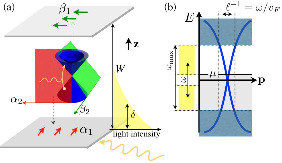
Besides the bulk PGE that can be understood in terms of infinite-system models, the PGE has been explored at the surfaces of metals Alperovich et al. 1981; Magarill and Ehntin 1981; Moore and Orenstein 2010 and topological insulators Hosur 2011; Junck et al. 2013; Lindner et al.; Kim et al. 2017, in which case the surface-normal component of (but not that of ) vanishes. In the field of WSMs, recently there was evidence from experiments and first principles calculations that Fermi arc states might play an important role in the photogalvanic response Wang et al. 2019; Chang et al. 2020, a contribution that was neglected in previous theories. In particular, Chang et al. 2020 have shown that the contribution of surface states to the PGE due to excitations between the surface states of the same surface are possible in some crystals due to a non-linear dispersion of those surface states.
The mere presence of surface states, however, does not capture the full peculiarity of a WSM. Importantly, the two-dimensional Fermi-arc surface states, constituting in some sense the reaction of a pair of chiral Weyl fermions to confinement, are tightly glued to the three-dimensional Weyl fermions Haldane, as illustrated in Fig. 1(a). This connectivity distinguishes Fermi arcs from surface states of metals and topological insulators and was shown to give rise to a number intriguing, counter-intuitive linear-response effects Burkov 2014; Moll et al. 2016; Wang et al. 2017; Behrends et al. 2019; Zhang et al. 2019b; Sukhachov et al. 2019; Breitkreiz and Brouwer 2019; Kaladzhyan and Bardarson 2019; Zhang et al. 2021; Breitkreiz 2020; Perez-Piskunow et al. 2021. Understanding its role also for the photogalvanic response is highly desirable. The theoretical challenge to capture the effect of the connectivity is the requirement to go beyond an effective surface theory and consider a full three-dimensional, yet spatially confined model.
In this work we present a theory of ballistic photogalvanic response of Weyl fermions spatially confined in one direction with general boundary conditions, relevant for Weyl-semimetal slabs with an arbitrary configuration of Weyl nodes and arbitrary orientations of Fermi arcs at the bottom and top surfaces, which need not be the same.
Specifically, the orientation of the bottom (top) Fermi arc is defined by the direction of its velocity, (), or the perpendicular direction at which the arc emanates from the Weyl node, (-), see Fig. 1(a). We show that this symmetry-breaking directionality gives rise to a vastly richer response behavior compared to an unconfined WSM. In particular, the confinement enables the otherwise vanishing linear and circular PGE in centrosymmetric WSMs. Furthermore, the response is crucially determined by the orientations of the Fermi arcs. The latter may be adjusted by choosing different surface terminations Morali et al. 2019; Fujii et al. 2021 or surface doping Li and Andreev 2015. In principle, this allows control over the photogalvanic response by modification of the surface only.
To focus on Weyl physics, we consider a photonfrequency range for which excitations can take place only close to Weyl nodes where the bulk and arc dispersions are linear, see Fig. 1(b). The total response is then the sum of the responses of individual Weyl nodes. Further, we focus on the semimetallic regime, in which the Fermi level is close to the Weyl node and smaller than the photon energy, such that Pauli blocking as well as screening may be neglected. In this regime, intra-surface (arc-arc) excitations are forbidden, but bulk-bulk excitations as well as arc-bulk excitations exist.
Most strikingly, for a centrosymmetric WSM confined to a slab, the photogalvanic response is fully determined by the Fermi-arc orientation. Considering the current density in Eq. (1) as the current density averaged over the slab width, the response tensor can be decomposed into a confinement-independent bulk-bulk contribution and confinement-induced contributions, which in turn consist of bulk-bulk as well as arc-bulk parts,
| (2) |
For a centrosymmetric WSM, vanishes according to general symmetry considerations Belinicher and Sturman 1980. The response is thus given by
| (3) |
where both contributions are fully determined by the Fermi-arc orientations since the orientation of the arcs and modification of the bulk-state wavefunctions are both defined by the boundary conditions. Moreover, a centrosymmetric WSM necessarily breaks time-reversal symmetry, which implies that will include a ballistic response to linearly polarized light of the type discussed in Zhang et al. 2019a. This is directly relevant to magnetic WSMs, such as Liu et al. 2018, Rees et al. 2020, and Suzuki et al. 2016. Table 1 summarizes which types of photogalvanic response are possible in unconfined and confined WSMs, depending on the mechanism and the presence of time-reversal and inversion symmetry.
| symmetry | time reversal | inversion | neither |
|---|---|---|---|
| (broken inversion) | (broken time reversal) | ||
| ballistic current (injection) | bCPGE, sCPGE | sCPGE, sLPGE | bCPGE, bLPGE, sCPGE, sLPGE |
| shift current | bLPGE, sLPGE | (sCPGE, sLPGE) | (bCPGE, bLPGE, sCPGE, sLPGE) |
Finally, the confinement-induced PGE is categorized depending on the slab thickness. For a sufficiently thick slab or sufficiently high frequency the light field does not penetrate the whole slab. This is the case when the penetration depth , which for photon energies to lies in the range to , is much smaller than the slab thickness . For light incident at the bottom surface, see Fig. 1(a), the top surface no longer contributes to the response. This changes the symmetry of the response tensor. We refer to this limit as the thick slab. In the opposite limit, referred to as the thin slab, , both surfaces contribute. Technically, the two limits require substantially different calculations, we will thus mostly consider the thick- and thin-slab regimes separately, using different analytical and numerical techniques.
This article is organized as follows. In Sec. II we introduce the model of a WSM in the slab geometry for which we perform our calculations. We also briefly discuss the decay of light waves in WSMs. Finally, we present the semiclassical formulae for the photogalvanic current that we employ. In Sec. III we classify the different contributions to the photogalvanic response tensor and estimate their magnitude. Further, we comment on the irrelevance of finite light momentum. In Sec. IV we discuss the symmetry constraints on the response tensor. Finally, in Sec. V we present analytical results for the different contributions to the response tensor for a single Weyl cone in the different regimes. We further present a lattice simulation in the thin limit which confirms the analytical results. At the end of this section we apply our results to WSMs with several Weyl cones by considering a centrosymmetric WSM with two nodes. We conclude in Sec. VI. Technical details are delegated to the appendices.
II Model
II.1 Weyl semimetal
We consider a WSM slab with a set of Weyl nodes which are close to the Fermi level and well-separated in momentum space. Since we consider the response to excitations occurring close to the Weyl nodes only, it suffices to consider the response of a single Weyl node, from which the response of a WSM with several Weyl nodes will follow by combining the single-Weyl-node response tensors, transformed according to the specific Weyl-node arrangement.
In order to evaluate the matrix elements relevant for the photogalvanic response tensors we seek explicit expressions for the wave-functions in the slab geometry (see Appendix A for a detailed derivation). To this end, we model a single Weyl fermion confined to with the Hamiltonian (we set )
| (4) |
where is the momentum (with ), the spin, the chirality, and the velocity. For better transparency of the following calculations we here assume isotropic velocity of the Weyl fermion; in Appendix B we generalize the results to an anisotropic Weyl node, which leads to a simple transformation of the response tensor. In the absence of a tilt, the Weyl Hamiltonian Eq. 4 commutes with the operator , where is complex conjugation. By analogy with relativistic theory we refer to this intra-node symmetry as time reversal (TR) symmetry. Note that it does not correspond to the time reversal operation acting on the whole crystal, as this connects different Weyl nodes. Thus the intra-node TR symmetry allows to constrain the response due to a single Weyl node only. A WSM with several Weyl nodes at generic points in momentum space clearly does not need to satisfy TR symmetry.
Using translation invariance parallel to the surface we seek energy eigenstates in the form of plane waves in the plane with the continuous in-plane momenta . Their dependence on is given by the solutions to the Weyl equation , which may be written as
| (5) |
where and the generalized momentum operator reads
| (6) |
The discrete energy eigenvalues of the slab (at fixed ) are to be determined by boundary conditions. A generic boundary condition on the wavefunction is a vanishing current across the boundaries. Since this corresponds to . Accounting for the possibility of differing boundary conditions for the bottom and top surfaces, a general boundary condition thus reads
| (7) |
parametrized by two independent angles and . Surface inhomogeneities would correspond to a spatial dependence of and . Here we assume translation invariance at the surface (up to a relaxation mean free path that will be introduced perturbatively below) and thus consider and to be constant.
The boundary conditions lead to the equation
| (8) |
which determines the quantized eigenvalues . Solutions with real correspond to bulk states, imaginary solutions correspond to surface “arc” states. For details and explicit expressions of the arc and bulk states see App. A. Note that and define the velocity of the Fermi arcs localized at the bottom (b) and top (t) surfaces,
| (9) |
as well as the direction at which they emanate from the Weyl node, given by the constraint
| (10) |
for bottom and top arc, respectively, where we defined the vectors
| (11a) | ||||
| (11b) | ||||
The quantities and introduced in Eq. (10) have the meaning of inverse decay lengths of the evanescent wave functions of arc states at the top and bottom surfaces respectively.
In order to analyze symmetries in the presence of the boundary conditions, it proves helpful to define an equivalent multilayer setup, which reproduces the same spectrum and wave-functions as the boundary conditions Eq. (7). Note that this is a fictitious system only introduced to assist in understanding the response of a single Weyl node. The equivalent multilayer setup is defined by the Hamiltonian
| (12) |
with Berry and Mondragon 1987; Bovenzi et al. 2018. Under TR the multilayer Hamiltonian transforms like
| (13) |
The mass terms of the boundary conditions thus behave like TR-breaking magnetizations in the directions and at the two boundaries. Note that this does not imply TR-breaking of the WSM with several Weyl nodes.
Furthermore, note that the directions of the boundary spinors can be additionally controlled by TR-preserving boundary potentials Li and Andreev 2015. One can easily check that adding a boundary potential to the Hamiltonian (12), rotates the boundary spinors like and . Boundary potentials are typically disregarded in minimal models of Weyl-semimetal slabs, which corresponds to straight arcs connecting the Weyl cones, i.e., . Here we instead consider the general case that the Fermi arcs can emanate in any direction, considering the boundary spinors (7) to be given by two independent variables and . The resulting curvature of Fermi arcs, which is necessary to connect pairs of Weyl nodes and is often observed in experiments, is irrelevant in the close vicinity of the Weyl nodes to which the optical transitions that we consider are bound.

The directionality introduced by the boundary conditions will crucially determine the direction of the response. It is therefore convenient to define the coordinate axes along the emergent high-symmetry directions. Those depend on whether current is induced at a single surface (thick-slab case) or in the whole slab (thin-slab case). Figure 2 illustrates the geometry and the high-symmetry axes in these two cases.
II.2 Electromagnetic waves in Weyl semimetals
For frequencies the conductivity in WSMs is given by Hosur et al. 2012; Steiner et al. 2017
| (14) |
Here, is the total number of Weyl nodes in the system, is the permittivity due to inert bands and we let to account for screening. Finally, we defined the dimensionless coupling constant
| (15) |
Note that takes values between and in a WSM, depending on the number of nodes. The imaginary part of has only weak frequency dependence and has been absorbed into . The frequency dependent permittivity then reads
| (16) |
We consider light entering the WSM at the surface. The field inside the WSM has the form,
| (17) |
where is the momentum inside the medium and is the penetration depth. In terms of the vacuum wavenumber and to leading order in , they are given by
| (18a) | ||||
| (18b) | ||||
With the above estimate of , depending on the number of Weyl nodes, we thus obtain .
II.3 Photogalvanic response tensor
We consider the response of the Weyl slab to the weak external oscillating electric field
| (19) |
In the temporal gauge , the perturbation to the Hamiltonian reads
| (20) |
where is the current operator and is the smallest length scale of our model. In the following we will use dimensionless length and momenta, denoted with a tilde,
| (21) |
in units of and , respectively.
The ballistic PGE can be described within the framework of the Boltzmann kinetic equation by balancing asymmetric photogeneration and impurity-induced relaxation. Using the standard perturbation theory and relaxation-time approximation, one can express the photogalvanic response in terms of the momentum relaxation time in the form Chan et al. 2017
| (22) |
where , , , and we introduced the matrix elements
| (23) |
and the constant (restoring , which is set to one)
| (24) |
These expressions hold for both bulk-bulk and and arc-bulk excitations. To avoid overcounting of states, for bulk states the sum runs only over while for arc states it runs over . Note that as for all states due to the boundary conditions.
Note that the three matrices are hermitian. According to standard terminology, the imaginary anti-symmetric part is associated with the circular PGE, which is present only if the incident light is elliptically polarized (the inverse implication is not true: elliptically polarized light can give rise to photogalvanic response stemming from the real symmetric part). The real symmetric part is referred to as the linear photogalvanic response, which exists even for linearly polarized radiation.
III Classification and estimate of response contributions
There are three relevant length scales in the problem 11 1 Here we neglect one length scale of the problem, which is the mean free path given by the relaxation time . Within the semiclassical approach described in Sec. II.3 the mean free path is assumed long compared to essentially all other relevant scales, which makes the mean free path itself irrelevant for the following discussion., the -weighted light wavelength , the light penetration depth , and the slab thickness , whereby the weighted light wavelength is always much smaller than the penetration depth, . The width is considered in two limits, the thick-slab case and the thin-slab case . In the thick-slab case the light completely decays inside the slab and only a single slab surface is excited. In the thin-slab case the light penetrates nearly homogeneously the whole slab such that both surfaces are equally excited. In this limit, for simplicity of analytical calculations we introduce a lower bound for the width, , so that energy quantization of slab modes is small compared to the light frequency. The ultrathin case will be considered numerically on a lattice model.
Before coming to the detailed calculation, it is useful to classify the response contributions according to their dependencies on the relevant length scales (, , ), separating confinement-independent from confinement-induced contributions and distinguishing contributions due to arc-bulk and bulk-bulk excitations as given in (2). The result is summarized in Table 2 and is explained in the following.
| thick slab | thin slab | |
|---|---|---|
| , |
To estimate the magnitudes of contributions it suffices to disregarding the spin degree of freedom and consider the bulk wavefunctions to be of the form and that of arc states of the form . In the latter, the inverse decay length , given in (10), has been approximated by the typical inverse distance from the Weyl node in the active region of excitations, which is set by . Neglecting the in-plane light momentum (will be justified below), the matrix elements (23) for the thick-slab case can be estimated as
| (25) |
The momentum separation of modes is , hence the number of modes within the active range around the node is . The summation over and thus gives
| (26) |
and the magnitude of the response tensor will thus scale like
| (27) |
for bulk-bulk and arc-bulk excitations, respectively.
Since , bulk-bulk excitations will give the dominant current contribution, while the confinement-induced correction due to arc-bulk excitations give the finite-size correction with the small parameter . Importantly, there are also contributions due to bulk-bulk excitations possible that scale like those from arc-bulk excitations,
| (28) |
To see this, note that the contribution stems from approximating the peaked behavior of the bulk-bulk matrix elements in (25) at by a delta function, the correction to setting is of the order because the peak width is and the effective integration range . Hence the leading correction scales like the arc-bulk contribution, and needs to be taken into account.
Upon changing the scales from the thick-slab case, , to the thin-slab case, , the scaling of the contribution of arc-bulk excitations does not change because the localization length of most arc states, given in (10), is set by and hence much smaller than both and .
For bulk-bulk excitations, the matrix elements are now the overlaps of wavefunctions over the whole slab width,
| (29) |
Summation over and gives and the magnitude of the current thus scales like
| (30) |
missing the factor as compared to the limit given in (27), since transitions are now produced across the full width of the slab.
As before, the matrix elements are peaked at ; the correction to the contribution is of order because the peak width is now , while the integration range is still . Thus remains valid also in the thin-slab limit. This concludes the explaination of the scaling summarized in Table 2.
III.1 Irrelevance of the light momentum
The momentum transfer due to a finite light momentum has the magnitude . The small parameter of corrections due to this momentum shift is , where is the typical momentum of excited states, hence . Comparing the smallness of corrections to the response, those due to a finite are irrelevant for the thin-slab case but potentially relevant in the case of a thick slab, where they are on the same order as the finite-size corrections, cf. Table 2. It turns out, however, that corrections to leading order in vanish also for the thick-slab case, which we show explicitly for our slab model in Appendix E. An easier way to find the same result is to realize that considering the correction due to a finite , one can neglect the finite-size corrections, which would give terms that are quadratic in the small parameter. Neglecting finite-size corrections, the result should thus coincide with that of an infinite system. In particular, the directionality introduced by the confinement becomes irrelevant. It is straightforward to verify that for a bulk Weyl cone the first-order corrections vanish.
For the response tensor in Eq. (II.3) this means that can be set to zero, the matrix elements become
| (31) |
and the momenta have the same parallel component, , .
IV Symmetry constraints
As the last preliminary consideration before coming to the explicit results, we now consider symmetry constraints on the response tensor. Considering the transition matrix elements (31) we realize that since the band index enters the wavefunctions in the form , which can be explicitly seen in Appendix A, Eq. (55), we obtain the relation
| (32) |
Using this and that other terms in the response expression, Eq. (II.3), are symmetric in , we conclude that
| (33) |
showing that the (anti)symmetric part of the response tensor is even (odd) in the chirality . Moreover, generally the (anti)symmetric part of the response tensor is odd (even) under TR Belinicher and Sturman 1980, which, according to the transformation behavior (13) is given by (in the fictitious multilayer system) and thus
| (34) |
For the thick-slab case, only the bottom surface is involved and corresponds to inversion of , i.e., mirror reflection with respect to the plane. Taking into account also symmetry with respect to , the response tensor assumes the form
| (35) |
For the thin-slab case, both surfaces are involved and combinations of two reflections leave the Hamiltonian invariant or time-reversed. In the thin-slab basis [Fig. 2(c)] we obtain
| (36a) | ||||
| (36b) | ||||
The resulting transformation behavior of the response tensor dictates the form
| (37) |
A more detailed derivation of the tensor forms is given in Appendix C.
V Results
V.1 PGE due to arc-bulk excitations

Arc-bulk excitations give rise to a current that is “automatically” a finite-size effect. Other finite-size corrections are negligible, which can be used to simplify the expression for the response tensor in Eq. (II.3); we can disregard the quantization of modes and replace the sums by integrals. The integration over in the matrix elements of Eq. (31) may be extended to infinity since the decay of surface modes at most momenta is on the order of , in both the thick-slab and thin-slab limits. Moreover we can neglect confinement-induced corrections of bulk states. A straightforward calculation (see Appendix D for details) then gives
| (38) |
for the bottom arc in the thick-slab basis , [Fig. 2(b)]. The antisymmetric part is expressed using the Levi-Civita symbol . This is the only arc-bulk contribution in the thick-slab case.
In the thin-slab case we add the contribution of the top arc, which is equivalent to the bottom arc up to the changed directions, , , see Fig. 2. Adding both contributions after appropriate rotation into the thin-slab basis [Fig. 2(c)] we obtain
| (39) |
where we defined
To understand this result, it suffices to understand the current production due to arc-bulk excitations at a single (bottom) surface, illustrated in Fig. 3. First we note that arc-bulk excitations vanish for the polarization component because such a photon does not act on the spinor of the arc (which is an eigenspinor of ) and thus cannot induce a transition to the orthogonal bulk state. This is circumvented when the linear polarization points in the other directions, and . The induced velocity due to arc-bulk excitations sum up to a total velocity pointing in the direction, see Fig. 3 (c), which explains the second term of (38).
Circular polarization instead acts like a ladder operator on the eigenspinor and thus enhances the amplitude of spin-flip excitations where the spin is increased (at positive in Fig. 3) and suppresses those where the spin is lowered (at negative in Fig. 3), and vice versa for the opposite polarization handedness, , or chirality of the Weyl fermions. As is clear from Fig. 3, this asymmetry can produce velocity in the direction, which sign depends on the polarization handedness and the chirality. This explains the first term of Eq. (38).
V.2 PGE due to bulk-bulk excitations
In contrast to the arc-bulk excitations, the contribution of excitations within the bulk bands (from the valence bulk band to the conduction bulk band) strongly differ for the thin- and thick-slab cases. We thus consider the two cases separately.

V.2.1 Thick slab limit
In this limit the light-induced excitations are produced at a single (bottom) surface in the finite strip of width . For the confinement-independent contribution we neglect all finite-size effects and obtain (see Appendix E.1 for details)
| (40) |
Apart from the absence of current in the direction perpendicular to the boundary and the factor , this expression is identical to the circular PGE found in the infinite system model Chan et al. 2017, which here has been re-derived using slab eigenstates. It is manifestly independent of the orientation of the Fermi arc. The prefactor correctly reflects the fact that excitations occur in the fraction of the penetration depth of the full sample width.
The leading corrections in the thick-slab limit are of a higher order in , see Table 2. They stem from the integration in the matrix elements (31), where we can still take the limit but keep the finite light penetration depth. Other finite-size corrections are controlled by the small parameter and can thus be neglected. Expansion to leading order in and numerical evaluation of the integral gives (see Appendix E.1 for details)
| (41) |
written in the thick-slab basis, , . We estimate that these expressions are accurate to below . Corrections to the circular PGE (antisymmetric part of the tensor) are in the same tensor components as the leading terms, as they should according to the symmetry constraints. The corrections are of opposite sign as the leading contribution because the tendency of the boundary to align the initial and final spinor suppresses the transition amplitude (circular PGE needs spin-flip processes). A difference between and components is a manifestation of the boundary-condition-broken symmetry between the and directions.
The response to linearly polarized light (symmetric part of the tensor) is something that is not found for an infinite-system Weyl cone in the absence of tilt. This follows from the fact that a single unconfined tiltless Weyl node is intra-node TR symmetric and hence there is no linear PGE. The vanishing of the linear PGE in such a system is due to cancellation of the linearly-polarized-light-induced current from states at opposite momenta parallel to the polarization Chan et al. 2017. While the symmetry considerations have already shown that linear PGE contributions are possible in the presence of a boundary, (which breaks intra-node TR symmetry) it is peculiar that these contributions stem not only from arc-bulk but also from bulk-bulk excitations. To understand how the boundary breaks the symmetry between opposite momenta of bulk states, we consider the bulk-state spinor as a function of , explicitly given in Eq. (55). At the boundary condition forces the spinors at all momenta to coincide with . Going away from the boundary, the spinors rotate in the in-plane basis: At small the spinor can be written as , with . Since , the rotation handedness is the same for all momenta and is set only by the chirality and the band (). The spin averaged over the whole slab width coincides with the spin of an infinite system—parallel or antiparallel to the momentum, depending on the band and chirality. As illustrated in Fig. 4, the angle between the spinor at and the averaged spinor, measured in the direction of rotation, thus always differs by for opposite momenta, which provides the crucial symmetry breaking and enables the response to linearly polarized radiation. Moreover, as can be seen from Eq. (55) and in Fig. 4(b), the (i.e., ) component of the spinor is invariant under simultaneous band change and , which explains the vanishing diagonal components for the response in the direction.
V.2.2 Thin slab
The confinement-independent contribution is obtained similarly to the thick-slab case by neglecting all finite-size corrections. The only difference is that the integration over now extends over the whole slab width instead of . The result,
| (42) |
is, up to the missing factor , identical to the thick-slab case and, up to the vanishing current normal to the slab, identical to the known infinite-system result, as it should.
For the confinement-induced contributions we collect finite-size corrections of the type . They stem from the quantization of and as well as from corrections to the wave functions and the velocity of bulk states. We solve the problem numerically via discretizing the polar angle , and finding pairs satisfying the energy conservation and Eq. (8) using standard numerical tools (see Appendix E.2 for details), yielding
| (43) |
where we defined
| (44) |
The numerical coefficients are accurate to the first decimal. Together with Eq. (38) and Eq. (41), Eq. (43) represents the central quantitative result of this work. Due to scale invariance of the Weyl Hamiltonian, these results are generic for any Weyl semimetal with untilted Weyl cones, up to straight-forward directional rescaling in case of anisotropic velocity, as discussed in Appendix B.
V.3 Discussion of confinement induced contributions and comparison to lattice simulation
The arc-bulk contribution and the confinement-induced bulk-bulk contribution are intimately linked: They are of the same order of magnitude and they always occur in combination. Therefore, only the sum is experimentally relevant.
In the thick-slab limit, the confinement-induced response tensor is
| (45) |
Note that since and cancel (within numerical accuracy), circularly polarized light may produce a sizeable current only parallel to the Fermi arc (), whereas linearly polarized light may produce currents perpendicular to the Fermi arc as well.

The thin slab limit result is plotted in Fig. 5 as a function of . For (), the linear PGE vanishes because the second surface restores the symmetry between opposite momenta: With regard to the corresponding discussion for the thick-slab limit, the sense of rotation of spinors away from the boundary is opposite to since runs “backwards” there. For () the symmetric part of the response tensor is approximately maximized, while the weight of circular response is simply shifted from one component to the other. The Fermi arc orientations thus change the nature of the response completely.
More generally, one can understand that the (anti)symmetric part of the tensor, i.e., the linear (circular) PGE, must be odd (even) in . In terms of , the TR-breaking directions in (12) are given by and . The transformation combined with the reflection and leaves the Hamiltonian invariant. From the corresponding transformation of the tensor follows that components of the symmetric part are odd while components of the anti-symmetric part are even in , as seen in Fig. 5.
While for clarity of the analysis we considered the thin-slab case assuming , it is possible to relax this constraint and consider ultrathin slabs with resorting to numerical techniques. Here, we used a one-dimensional lattice realization of a single Weyl node (discretizing the -direction while keeping continuous) to numerically evaluate the photogalvanic response tensor in Eq. (II.3). Details can be found in Appendix F. The results are shown in Fig. 6, demonstrating that our semi-analytical results can be reproduced in a lattice setting, and that the qualitative behaviour, such as sign and magnitude of the confinement induced contributions, extends down to . For , the finite-size gap of modes becomes larger than the photon energy and the response vanishes.

V.4 Centrosymmetric Weyl semimetal

Our results for a single Weyl node allow to infer on the response of a WSM with several nodes by adding the contributions of each node. Probably the most intersting case is that of centrosymmetric WSMs, for which the confinement-independent bulk-bulk contributions cancel and only the confinement-induced contributions, and , survive. A minimal model of a centrosymmetric bulk WSM consists of a single pair of Weyl nodes with opposite chirality. Considering the multilayer Hamiltonian in (12) as the Hamiltonian describing one of the Weyl nodes, for the Hamiltonian describing the second Weyl node of opposite chirality we take . In this case the Fermi arcs emanate in opposite directions, which happens when the Weyl nodes are connected in a straight line. However, we have seen in Sec. II that an additional boundary potential rotates the spinors by and . The generic situation is thus that there is a finite angle characterizing the deviation from an anti-parallel alignment, as shown in the inset of Fig. 7(a). Note that between the nodes, the Fermi arcs thus must be curved, as is typically seen in experiments; the curvature itself plays however no role for our results since excitations occur only close to the Weyl nodes.
The total response is obtained from the single-cone result (now explicitly denoting the dependence),
| (46) |
where is the spatial rotation matrix for a rotation around by . The results are plotted in Fig. 7. From the transformation behavior of the response tensor discussed in Sec. IV (symmetric part odd in and even in , antisymmetric part odd in and even in ), the response of the two Weyl nodes cancel each other at . This means that in the thick-slab case the response vanishes when the Fermi arcs of the illuminated surface emanate from the Weyl nodes in exactly opposite directions. In the thin-slab case, the same applies but the emanation direction is replaced by the bisector of the top- and bottom-surface Fermi arcs.
For the directions just discussed (emanation direction for thick slab and bisector direction for thin slab) are parallel. This is equivalent to taking the contributions of the two Weyl nodes at the same (instead of and ), while are still opposite. Since the (anti)symmetric part is even (odd) in , the antisymmetric parts cancel also here but the symmetric parts add up to twice the value of a single cone. This can be seen by comparison of Fig. 7(b) with the single-cone results shown in Fig. 5 for the thin-slab case and Fig. 7(a) with from Eqs. (38) and (41) for the thick-slab case. (Note that the coordinate system is now rotated by , i.e., and , compared to the single-cone case).
VI Conclusion
In conclusion, we have explored the PGE of a WSM spatially confined to a slab geometry. Symmetry breaking on the surfaces via the orientation of the Fermi arcs enables circular and linear photogalvanic response currents, which would otherwise not be possible, in particular, in centrosymmetric WSMs.
The magnitude of the confinement-enabled PGE inherits the topology-enhancement of an unconfined Weyl Fermion, based on the topologically protected band touchings. However, while in infinite systems those band touchings include only the chiral pairs of Weyl nodes, a confined system features topological surface states, which are tightly glued to the Weyl nodes.
The ratio of confinement-induced contributions to bulk contributions scales in case of a thin slab like and for the thick slab like , where is the light wavelength, the slab thickness, and the node- vs. light-velocity. Considering the upper and lower bounds of set by the finite Fermi level and the band width of typical WSM materials, the confinement-induced PGE is on the order of bulk PGE for widths of order m. Surface-controlled PGE is thus found in such thin slabs even for non-centrosymmetric WSMs, which makes the experimental realization of thin WSM slabs or even stacks of those especially interesting.
One of the most remarkable properties of the confinement-induced PGE is that it is controlled by surface boundary conditions. We explicitly discussed the effect of a surface potential, which rotates the direction of Fermi arcs. Another interesting possibility, known from experiments, are layered WSMs for which the different surface terminations can not only change the directionality of Fermi arcs but even lead to different connectivities to the Weyl nodes Morali et al. 2019; Fujii et al. 2021. This Fermi-arc geometry is observable, e.g., via angle-resolved photoemission spectroscopy Xu et al. 2015a; Xu et al. 2015b; Yang et al. 2015; our work links this geometry with the photogalvanic response.
With regard to the remarkable recent progress in device microstructuring Moll 2018; Zhang et al. 2019b; Nishihaya et al. 2019; Bedoya-Pinto et al. 2020; Qin et al. 2020, our work might thus play an important role in identifying Weyl physics and shaping the photogalvanic response by designing the material surface.
Note added
When this work was substantially completed, we became aware of a recent article Cao et al. considering the PGE of a finite system using a minimal centrosymmetric lattice model that features two Weyl nodes. This article focuses on Fermi energies far away from the Weyl nodes where the PGE is governed by non-linear terms of the dispersion, while in the semimetallic regime, which is the focus of our work, the response of their model vanishes as it, in terms of our model, considers only the specific case of Sec. V.4. This trivial case is the only place of overlap of our works.
Acknowledgements.
We benefited from a discussion with Haim Beidenkopf. J. F. S. gratefully acknowledges financial support by QuantERA project Topoquant, as well as by the Deutsche Forschungsgemeinschaft (DFG, German Research Foundation) through Priority Program 1666 and CRC 910. M. B. was funded by Grant No. 18688556 of the DFG. The work of A. A. was supported by the National Science Foundation Grant MRSEC DMR-1719797.References
- Wan et al. (2011) X. Wan, A. M. Turner, A. Vishwanath, and S. Y. Savrasov, Phys. Rev. B 83, 205101 (2011).
- Lv et al. (2015) B. Lv, H. Weng, B. Fu, X. Wang, H. Miao, J. Ma, P. Richard, X. Huang, L. Zhao, G. Chen, Z. Fang, X. Dai, T. Qian, and H. Ding, Phys. Rev. X 5, 031013 (2015).
- Yang et al. (2015) L. X. Yang, Z. K. Liu, Y. Sun, H. Peng, H. F. Yang, T. Zhang, B. Zhou, Y. Zhang, Y. F. Guo, M. Rahn, D. Prabhakaran, Z. Hussain, S.-K. Mo, C. Felser, B. Yan, and Y. L. Chen, Nat. Phys. 11, 728 (2015).
- Xu et al. (2015a) S.-Y. Xu, N. Alidoust, I. Belopolski, Z. Yuan, G. Bian, T.-R. Chang, H. Zheng, V. N. Strocov, D. S. Sanchez, G. Chang, C. Zhang, D. Mou, Y. Wu, L. Huang, C.-C. Lee, S.-M. Huang, B. Wang, A. Bansil, H.-T. Jeng, T. Neupert, A. Kaminski, H. Lin, S. Jia, and M. Zahid Hasan, Nat. Phys. 11, 748 (2015a).
- Xu et al. (2015b) S.-Y. Xu, C. Liu, S. K. Kushwaha, R. Sankar, J. W. Krizan, I. Belopolski, M. Neupane, G. Bian, N. Alidoust, T.-R. Chang, H.-T. Jeng, C.-Y. Huang, W.-F. Tsai, H. Lin, P. P. Shibayev, F.-C. Chou, R. J. Cava, and M. Z. Hasan, Science 347, 294 (2015b).
- Hosur et al. (2012) P. Hosur, S. A. Parameswaran, and A. Vishwanath, Phys. Rev. Lett. 108, 046602 (2012).
- Burkov (2018) A. A. Burkov, Annu. Rev. Condens. Matter Phys. 9, 359 (2018).
- Adler (1969) S. L. Adler, Phys. Rev. 177(5), 2426 (1969).
- Bell and Jackiw (1969) J. S. Bell and R. W. Jackiw, Nuovo Cim. 60, 47 (1969).
- Nielsen and Ninomiya (1983) H. B. Nielsen and M. Ninomiya, Phys. Lett. B 130(6), 389 (1983).
- Balents (2011) L. Balents, Physics (College. Park. Md). 4, 36 (2011).
- Liu et al. (2020) J. Liu, F. Xia, D. Xiao, F. J. García de Abajo, and D. Sun, Nat. Mater. 19, 830 (2020).
- Guan et al. (2021) M.-X. Guan, E. Wang, P.-W. You, J.-T. Sun, and S. Meng, Nat. Commun. 12, 1885 (2021).
- Armitage et al. (2018) N. P. Armitage, E. J. Mele, and A. Vishwanath, Rev. Mod. Phys. 90, 015001 (2018).
- Taguchi et al. (2016) K. Taguchi, T. Imaeda, M. Sato, and Y. Tanaka, Phys. Rev. B 93, 201202 (2016).
- Morimoto et al. (2016) T. Morimoto, S. Zhong, J. Orenstein, and J. E. Moore, Phys. Rev. B 94, 245121 (2016).
- Chan et al. (2017) C.-K. Chan, N. H. Lindner, G. Refael, and P. A. Lee, Phys. Rev. B 95, 041104 (2017).
- König et al. (2017) E. J. König, H.-Y. Xie, D. A. Pesin, and A. Levchenko, Phys. Rev. B 96, 075123 (2017).
- Golub et al. (2017) L. E. Golub, E. L. Ivchenko, and B. Z. Spivak, JETP Lett. 105, 782 (2017).
- Sun et al. (2017) K. Sun, S.-S. Sun, L.-L. Wei, C. Guo, H.-F. Tian, G.-F. Chen, H.-X. Yang, and J.-Q. Li, Chin. Phys. Lett. 34, 117203 (2017).
- Ma et al. (2017) Q. Ma, S.-Y. Xu, C.-K. Chan, C.-L. Zhang, G. Chang, Y. Lin, W. Xie, T. Palacios, H. Lin, S. Jia, P. A. Lee, P. Jarillo-Herrero, and N. Gedik, Nat. Phys. 13, 842 (2017).
- Zhang et al. (2018) Y. Zhang, H. Ishizuka, J. van den Brink, C. Felser, B. Yan, and N. Nagaosa, Phys. Rev. B 97, 241118 (2018).
- Ahn et al. (2020) J. Ahn, G.-Y. Guo, and N. Nagaosa, Phys. Rev. X 10, 041041 (2020).
- Watanabe and Yanase (2021) H. Watanabe and Y. Yanase, Phys. Rev. X 11, 11001 (2021).
- Belinicher and Sturman (1980) V. I. Belinicher and B. I. Sturman, Soviet Physics Uspekhi 23, 199 (1980).
- Ivchenko and Pikus (2012) E. Ivchenko and G. Pikus, Superlattices and Other Heterostructures: Symmetry and Optical Phenomena, Springer Series in Solid-State Sciences (Springer Berlin Heidelberg, 2012).
- Sipe and Shkrebtii (2000) J. E. Sipe and A. I. Shkrebtii, Phys. Rev. B 61, 5337 (2000).
- de Juan et al. (2017) F. de Juan, A. G. Grushin, T. Morimoto, and J. E. Moore, Nat. Commun. 8, 15995 (2017).
- Rees et al. (2020) D. Rees, K. Manna, B. Lu, T. Morimoto, H. Borrmann, C. Felser, J. E. Moore, D. H. Torchinsky, and J. Orenstein, Sci. Adv. 6, eaba0509 (2020).
- Osterhoudt et al. (2019) G. B. Osterhoudt, L. K. Diebel, M. J. Gray, X. Yang, J. Stanco, X. Huang, B. Shen, N. Ni, P. J. W. Moll, Y. Ran, and K. S. Burch, Nat. Mater. 18, 471 (2019).
- Zhang et al. (2019a) Y. Zhang, T. Holder, H. Ishizuka, F. de Juan, N. Nagaosa, C. Felser, and B. Yan, Nat. Commun. 10, 3783 (2019a).
- Holder et al. (2020) T. Holder, D. Kaplan, and B. Yan, Phys. Rev. Research 2, 033100 (2020).
- Fei et al. (2020) R. Fei, W. Song, and L. Yang, Phys. Rev. B 102, 035440 (2020).
- Alperovich et al. (1981) V. L. Alperovich, V. I. Belinicher, V. N. Novikov, and A. S. Terekhov, Zh. Eksp. Teor. Fiz. 80, 2298 (1981).
- Magarill and Ehntin (1981) L. I. Magarill and M. V. Ehntin, Zh. Eksp. Teor. Fiz. 81, 1001 (1981).
- Moore and Orenstein (2010) J. E. Moore and J. Orenstein, Phys. Rev. Lett. 105, 026805 (2010).
- Hosur (2011) P. Hosur, Phys. Rev. B 83, 035309 (2011).
- Junck et al. (2013) A. Junck, G. Refael, and F. von Oppen, Phys. Rev. B 88, 075144 (2013).
- (39) N. H. Lindner, A. Farrell, E. Lustig, G. Refael, and F. von Oppen, arXiv:1403.0010 .
- Kim et al. (2017) K. W. Kim, T. Morimoto, and N. Nagaosa, Phys. Rev. B 95, 035134 (2017).
- Wang et al. (2019) Q. Wang, J. Zheng, Y. He, J. Cao, X. Liu, M. Wang, J. Ma, J. Lai, H. Lu, S. Jia, D. Yan, Y. Shi, J. Duan, J. Han, W. Xiao, J.-H. Chen, K. Sun, Y. Yao, and D. Sun, Nat. Commun. 10, 5736 (2019).
- Chang et al. (2020) G. Chang, J.-X. Yin, T. Neupert, D. S. Sanchez, I. Belopolski, S. S. Zhang, T. A. Cochran, Z. Chéng, M.-C. Hsu, S.-M. Huang, B. Lian, S.-Y. Xu, H. Lin, and M. Z. Hasan, Phys. Rev. Lett. 124, 166404 (2020).
- (43) F. D. M. Haldane, arXiv:1401.0529 .
- Burkov (2014) A. A. Burkov, Phys. Rev. Lett. 113, 187202 (2014).
- Moll et al. (2016) P. J. W. Moll, N. L. Nair, T. Helm, A. C. Potter, I. Kimchi, A. Vishwanath, and J. G. Analytis, Nat. Lett. 535, 266 (2016).
- Wang et al. (2017) C. M. Wang, H. P. Sun, H. Z. Lu, and X. C. Xie, Phys. Rev. Lett. 119, 136806 (2017).
- Behrends et al. (2019) J. Behrends, R. Ilan, and J. H. Bardarson, Phys. Rev. Res. 1, 032028 (2019).
- Zhang et al. (2019b) C. Zhang, Z. Ni, J. Zhang, X. Yuan, Y. Liu, Y. Zou, Z. Liao, Y. Du, A. Narayan, H. Zhang, T. Gu, X. Zhu, L. Pi, S. Sanvito, X. Han, J. Zou, Y. Shi, X. Wan, S. Y. Savrasov, and F. Xiu, Nat. Mater. 18, 482 (2019b).
- Sukhachov et al. (2019) P. O. Sukhachov, M. V. Rakov, O. M. Teslyk, and E. V. Gorbar, Ann. Phys. 532, 1900449 (2019).
- Breitkreiz and Brouwer (2019) M. Breitkreiz and P. W. Brouwer, Phys. Rev. Lett. 123, 066804 (2019).
- Kaladzhyan and Bardarson (2019) V. Kaladzhyan and J. H. Bardarson, Phys. Rev. B 100, 085424 (2019).
- Zhang et al. (2021) C. Zhang, Y. Zhang, H.-Z. Lu, X. C. Xie, and F. Xiu, Nat. Rev. Phys. 3, 660 (2021).
- Breitkreiz (2020) M. Breitkreiz, Phys. Rev. Res. 2, 012071(R) (2020).
- Perez-Piskunow et al. (2021) P. M. Perez-Piskunow, N. Bovenzi, A. R. Akhmerov, and M. Breitkreiz, SciPost Phys. 11, 46 (2021).
- Morali et al. (2019) N. Morali, R. Batabyal, P. K. Nag, E. Liu, Q. Xu, Y. Sun, B. Yan, C. Felser, N. Avraham, and H. Beidenkopf, Science 365, 1286 (2019).
- Fujii et al. (2021) J. Fujii, B. Ghosh, I. Vobornik, A. Sarkar, D. Mondal, C. Kuo, F. Bocquet, D. Boukhvalov, C. S. Lue, A. Agarwal, and A. Politano, ACS Nano (2021), 10.1021/acsnano.1c04766.
- Li and Andreev (2015) S. Li and A. V. Andreev, Phys. Rev. B 92, 201107 (2015).
- Liu et al. (2018) E. Liu, Y. Sun, N. Kumar, L. Muechler, A. Sun, L. Jiao, S.-Y. Yang, D. Liu, A. Liang, Q. Xu, J. Kroder, V. Süß, H. Borrmann, C. Shekhar, Z. Wang, C. Xi, W. Wang, W. Schnelle, S. Wirth, Y. Chen, S. T. B. Goennenwein, and C. Felser, Nat. Phys. 14, 1125 (2018).
- Suzuki et al. (2016) T. Suzuki, R. Chisnell, A. Devarakonda, Y.-T. Liu, W. Feng, D. Xiao, J. Lynn, and J. Checkelsky, Nat. Phys. 12, 1119 (2016).
- Berry and Mondragon (1987) M. V. Berry and R. J. Mondragon, Proc. R. Soc. London A 412, 53 (1987).
- Bovenzi et al. (2018) N. Bovenzi, M. Breitkreiz, T. E. O’Brien, J. Tworzydło, and C. W. J. Beenakker, New J. Phys. 20, 023023 (2018).
- Steiner et al. (2017) J. Steiner, A. Andreev, and D. Pesin, Phys. Rev. Lett. 119, 036601 (2017).
- (63) Here we neglect one length scale of the problem, which is the mean free path given by the relaxation time . Within the semiclassical approach described in Sec. II.3 the mean free path is assumed long compared to essentially all other relevant scales, which makes the mean free path itself irrelevant for the following discussion.
- Moll (2018) P. J. Moll, Annu. Rev. Condens. Matter Phys. 9, 147 (2018).
- Nishihaya et al. (2019) S. Nishihaya, M. Uchida, Y. Nakazawa, R. Kurihara, K. Akiba, M. Kriener, A. Miyake, Y. Taguchi, M. Tokunaga, and M. Kawasaki, Nat. Commun. 10, 2564 (2019).
- Bedoya-Pinto et al. (2020) A. Bedoya-Pinto, A. K. Pandeya, D. Liu, H. Deniz, K. Chang, H. Tan, H. Han, J. Jena, I. Kostanovskiy, and S. S. Parkin, ACS Nano 14, 4405 (2020).
- Qin et al. (2020) P. Qin, Z. Feng, X. Zhou, H. Guo, J. Wang, H. Yan, X. Wang, H. Chen, X. Zhang, H. Wu, Z. Zhu, and Z. Liu, ACS Nano 14, 6242 (2020).
- (68) J. Cao, M. Wang, Z.-M. Yu, and Y. Yao, arXiv:2108.08138 .
Appendix A Confined Weyl Fermion wave functions
In this appendix we derive the explicit form of the eigenfunctions of Eq. (4) in the slab geometry . Writing the momentum operator in the spatial basis, the Weyl equation can be written as
| (47) |
where the generalized momentum was defined in Eq. (6). The Weyl equation is formally solved by Eq. (II.1). Defining an orthonormal basis for our model of zero out-of-plane current states,
| (48) |
the generic boundary conditions at the two surfaces can be written as
| (49) |
From the boundary conditions, the quantized eigenvalues are the solutions of
| (50) |
where is in the basis of Fig. 2(c). Solutions with real correspond to bulk states, imaginary solutions correspond to surface “arc” states, which we will now discuss in more detail.
A.1 Arc states
For an imaginary , normalizable wavefunctions are found that are localized at the bottom (b) and top (t) surfaces,
| (51a) | ||||
| (51b) | ||||
(These expressions assume for ). From the criterion of normalizability, the momenta of Fermi arcs are bound to
| (52) |
The dispersion relations read
| (53) |
and hence the velocity expectation values are
| (54) |
The directions and are thus the directions in which the Fermi arcs emanate from the Weyl node () and the directions of their motion (), both up to the sign, as indicated in Fig. 2.
A.2 Bulk states
For a real , from (II.1) the normalized wavefunctions of the conduction and valence band read
| (55) |
where the normalization factor, isolating the finite-size correction , is given by
| (56a) | ||||
| (56b) | ||||
The velocity expectation values read
| (57a) | ||||
| (57b) | ||||
where we again isolated the finite-size correction , which stems from the weak dependence of the quantized , as implicitly given in (8). Note that due to the boundary conditions for all states.
Appendix B Anisotropic Weyl node
Here we generalize our calculations to Weyl fermions with anisotropic velocity. We consider the Hamiltonian
| (58) |
where and we defined in terms of
| (59) |
The chirality of the anisotropic Weyl node is . Undashed symbols refer to the isotropic case discussed in the main text. The current operator is
| (60) |
To avoid complications in the boundary condition we specify to
| (61) |
where is a 2x2 matrix acting only on components parallel to the boundary. Furthermore, we set . With this we may again employ the boundary conditions of Eq. (7). Then, the arc and bulk wave-functions may be obtained by simply replacing in Eqs. (51a), (51b) and Eq. (55). Similarly, the velocities can be expressed in terms of the isotropic expressions via
| (62) |
Altogether, the response tensor of the anisotropic Weyl node is related to the isotropic node via (c.f. Eq. (II.3))
| (63a) | ||||
| (63b) | ||||
| (63c) | ||||
where the determinant stems from the change of variables to (using due to our choice of ).
Appendix C Symmetry considerations
C.1 Thick slab
We work in the basis of the thick slab . The heterostructure Hamiltonian Eq. (12) of the semi-infinite system under consideration can be written as
| (64) |
where the vacuum at is modeled by a large mass term with , which acts like a magnetization in breaking the intra-node TR symmetry, as discussed in the main text. We consider spatial mirror-plane reflections , , with corresponding to reflection w.r.t. the plane, etc. A single reflection reverses the component of the momentum and the current that is normal to the mirror plane and the components of the spin that are parallel to the mirror plane. The action of the reflections on the Hamiltonian thus read
| (65) |
In words, reflection reverses the chirality and reflection reverses the chirality and the magnetization.
From this we can infer on the transformation behavior of the response tensor. First, note that the (anti)symmetric part of the response tensor, (), is generally odd (even) under TR Belinicher and Sturman 1980 – the (anti)symmetric part is thus odd (even) under . Second, in Sec. IV we have shown that the (anti)symmetric part of the response tensor is even (odd) under . Taking also into account the transformation of the current under reflections, we obtain for the symmetric part,
| (66a) | ||||
| (66b) | ||||
| (66c) | ||||
| (66d) | ||||
while the antisymmetric part satisfies
| (67a) | ||||
| (67b) | ||||
| (67c) | ||||
| (67d) | ||||
From this follows
| (68) |
C.2 Thin slab
We now work in the basis of the thin slab, depiceted in Fig. 2(c). We now consider the full heterostructure Hamiltonian (12),
| (69) |
with . The behavior under reflections and TR is as in the previous section but now with two TR-breaking magnetizations.
We consider two symmetry transformations. First we note that the combined reflection , which swaps the top and bottom surfaces, and , which interchanges and , leave the Hamiltonian invariant. Second, the combination of and inverts both and , which can be compensated by . Altogether,
| (70) |
Both the symmetric and the antisymmetric parts of the response tensor thus satisfy
| (71a) | ||||
| (71b) | ||||
and, since the symmetric part is odd under , it satisfies
| (72a) | ||||
| (72b) | ||||
while the antisymmetric part satisfies
| (73a) | ||||
| (73b) | ||||
From this follows,
| (74) |
Finally, we may also constrain the dependency of the components with respect to the angle . In terms of , the magnetization directions are given by and . First, note that the transformation may be compensated by . From this follows that components of the symmetric part of are odd under while components of the anti-symmetric part are even. Next note, that inverts both magnetizations and may be compensated by TR. From this follows that components of the symmetric part of are odd under while components of the anti-symmetric part are even.
Appendix D Photogalvanic current due to arc-bulk excitations
As explained in the main text, the leading-order current contribution due to arc-bulk excitations is of the same order of magnitude as the subleading contributions from bulk-bulk excitations. Other types of finite-size corrections that we had to account for when considering bulk-bulk excitations can now be disregarded, as they would give corrections of higher order. In particular, we can replace the momentum sum over by integrals in both the thick and thin slab regimes. Furthermore, we can assume and in both regimes and neglect the finite light momentum . In the thick slab limit only the bottom arc is relevant, in the thin slab limit both arcs contribute.
The response tensor due to the bottom arc is
| (75) |
where all momenta are dimensionless (in the appendix we suppress the tilde, which denotes dimensionless units in the main text). The first line captures transitions between conduction band and arc sheet, while the second captures transitions between the arc sheet and the valence band (the first Heaviside- function enforces normalizability of the arc states, the second allows transitions between empty and occupied states only). We also defined the arc-bulk matrix elements ()
| (76a) | ||||
| (76b) | ||||
Letting in the second term of Eq. (D) the current may be written as
| (77) |
This may be evaluated straightforwardly. The resulting response tensor in the thick slab basis is
| (78) |
The current due to the top arc (present only in the thin slab regime) may be obtained analogously. The result for the top arc in the basis , is
| (79) |
In the thin-slab case both contributions combine into the total arc-bulk contribution. Introducing the rotation operator
| (80) |
the total arc-bulk contribution, in the thin-slab basis [Fig. 2(c)], is given by
| (81) |
which evaluates to
| (82) |
Appendix E Photogalvanic current due to bulk-bulk excitations
This appendix section is structured as follows. First we perform some general manipulations. Next we discuss the thick and thin slab limits separately. In the thick slab limit, we may let and ignore the quantization condition Eq. (8). Corrections to the infinite system response arise from the spatial variation of the electromagnetic field corresponding to finite . These are of the same order of magnitude as the current due to arc-bulk excitations. Conversely, in the thin slab limit, the spatial dependence of the electromagnetic field may be ignored (), but the quantization condition due to finite leads to corrections of the same order as the arc-bulk current.
We start from Eq. (II.3) and specify to bulk states and ,
| (83) |
where we defined the dimensionless bulk-bulk matrix elements
| (84) |
Note that as opposed to the main text here we explicitly include the light momentum . Since , the light momentum is a factor smaller than the typical momenta of excited states . We will show below that it does not contribute at the relevant order of magnitude, in agreement with the argumentation in the main text. We set and keep terms to first order in .
We proceed by performing the integral over using the conservation of energy. The delta function gives the condition
This has a real solution if, to leading order in ,
| (85) |
where we defined new variables
| (86) |
with . The solution to is given by
| (87) |
Performing the integration over also gives rise to the Jacobian factor
| (88) |
The derivatives may be obtained from the boundary condition Eq. 50. They contribute at order . Altogether, the bulk-bulk response tensor is now
| (89) |
Next, consider the matrix elements, . We can split them into a normalization factor that is common to all and a factor that depends on ,
| (90) |
where the are defined in Eq. (56). Using
| (91) |
the read
| (92) |
where we defined as well as the integrals
| (93a) | ||||
| (93b) | ||||
These lead to conservation of “momentum” perpendicular to the boundary if or become large. It will prove convenient to also define the combinations
| (94) |
To leading order in , this gives
| (95) |
E.1 Thick slab
In this limit, dominant corrections are of order . They stem from the light penetration depth and the finite light momentum with . Ignoring the quantization of , which give corrections of order we replace
| (96) |
We expand the bulk-bulk current in orders of and .
E.1.1 Leading order bulk-bulk contributions
For the leading-order contributions we set (i.e., ) and analyze integrals of the type
| (97) |
which enter the current formula with a smooth kernel ( does not depend on the small parameter). Considering , we find
| (98) |
The leading contribution after integration is the term proportional to . Next, we use that
| (99) |
so that to leading order in and we can simplify
| (100) |
and are similar to with replaced by or , respectively. They clearly give the same leading order behaviour. For we have to leading order
| (101) |
Since is smooth, corrections from small are of higher order in .
Consider next and the corresponding cross-term. It is
| (102) |
Due to the extra factor of this may safely be ignored. However,
| (103) |
does not come with a small factor in the numerator at all. Naively one might expect a contribution of order . The factor of reduces this to a contribution of order . The leading order contribution stems from the lowest power in , i.e. the term proportional to . Then, integrating by parts
| (104) |
Here, we used
s.t. the integrand is again a delta function for . Hence, for
| (105) |
For the cross-term we find by a similar argument
| (106) |
which is again negligible.
Finally, consider cross-terms of the type , , , . The former two read to leading order
| (107) |
The latter two read
| (108) |
With this we can now easily calculate the bulk-bulk current in the thick slab limit at leading order. We drop all combinations with which do not give a order- contribution. The remaining combinations all give a delta function , corresponding to conservation of perpendicular momentum, , and hence and . Identifying the combinations giving rise to order- terms motivates the following definition:
| (109) |
where and . Here is (up to normalization) the matrix element at fixed momentum,
| (110) |
in terms of the spherical coordinates , , while
This term in the matrix element only arises if one allows for . It arises because may become large if even though they vanish for (or if the integral is cut off by the thickness of the slab, see below). The normalization factor evaluates to
| (111) |
Altogether, after transforming , we have
| (112) |
The angular integrals may be evaluated straightforwardly. This gives Eq. (40). Note that the result is symmetric under rotations in the -plane and thus independent of the direction of the boundary conditions.
E.1.2 Subleading order bulk-bulk contributions
We now consider the leading corrections to . From the above calculations, one can expect a correction of order
| (113) |
stemming from two different sources: first, from an in-plane momentum shift due to the finite light momentum , and second, from the corrections to the integrals of order . Consider first corrections due to finite light momentum. Since these are already of the same magnitude as the corrections due to finite-size as well as the arc-bulk current, one may ignore the slab geometry here. It is straightforward to verify that for a bulk Weyl cone these corrections vanish. We thus expect that the relevant corrections due to a finite vanish also in the slab. We first consider finite . The products do not involve and are thus approximated as in the leading-order calculation above. In we can thus again separate out and and expand the prefactors up to leading order in ,
| (114) |
where, introducing the shorthand notation ,
| (115a) | ||||
| (115b) | ||||
Other terms entering the current formula expand as
| (116a) | ||||
| (116b) | ||||
We now specify to the basis of the thick slab, . For (i.e., ) this combines to the total correction of the response tensor
It is straightforward to confirm that these expressions vanish upon integration over . Similar expressions for (i.e., ) also vanish.
The remaining corrections are corrections to the products , which have been discussed above, of order . We verified numerically, that the correction due to a finite vanishes as expected. Fitting the numerically evaluated response tensor (for ) to an expansion up to second order in we find (rounding to the second decimal)
To estimate the accuracy of these results we compare the numerical values given here to those obtained by fitting expansions to higher order in as well as by adding/removing data points corresponding to the smallest values of . These changes in the fitting procedure lead to changes in the numerical coefficients of . The error analysis is summarized in Table 3.
| Error |
E.2 Thin slab
In this limit, the leading finite-size corrections are , as discussed in the main text. Corrections due to the spatial variation of the external field, which we found to give corrections of order , are thus negligible and we can set . We now work in the basis of the thin slab.
E.2.1 Leading order ()
To calculate the leading order response we disregard the quantization of . Considering leading-order terms of the integral products , the dominant contributions read
| (119) |
all other combinations contribute only at higher order. Since the difference to the leading contribution of the thick-slab case is in the constant prefactor, the leading-order bulk-bulk contribution in the thin slab limit is given by the thick-slab result replacing . The final response tensor reads
| (120) |
E.2.2 Subleading order ()
The leading corrections to the bulk-bulk contribution in the thin slab limit are of order . They can stem from the quantization of , the associated corrections to the velocity in Eq. (57), and the corrections to the wavefunction normalization. The current is given by Eq. (89) with solutions of
| (121a) | ||||
| (121b) | ||||
where we defined the characteristic angle
| (122) |
These expressions as well as the tensors below are in the basis of the thin slab. Note that energy conservation makes and thus also and depend on . To evaluate the expression for the current for a given value of we resort to numerics. We then attempt to extract the functional dependence of the nonzero tensor components by fitting appropriate polynomials in and .
We briefly outline the numerical strategy employed to extract the response tensor. For -integration at fixed we employ standard numerical techniques relying on evaluation of the integrand for a discrete set of -points. For each -point we numerically determine all solutions to Eqs. (121) in the region . To determine we evaluate Eq. (89) at and subtract the leading order term, Eq. (120). We then fit to an expansion up to second order in and extract the coefficient of the term. In this way we determine all symmmetry-allowed elements of for 30 values of (the intervals and may be obtained from symmetry considerations, see Sec. C). Finally, we fit the components of the symmetric part of the response tensor to each element to an appropriate expansion in Fourier modes,
where we exploit that they are odd under and . Similarly, we fit the components of the anti-symmetric part to
where we use that they are even under the above transformations. We found that gives sufficiently good results with higher order coefficients satisfying . Rounding to , the subleading order response tensor due to bulk-bulk excitations in the thin slab limit is
These results are accurate to the first decimal: the error estimates of the numerical integration scheme are on the order of to . Similarly, altering the fitting procedure (e.g. by fitting to a first order expansion in or by removing data-points in ) leads to changes in the numerical coefficients on the order of roughly with the largest changes, at about , observed for the -independent terms in the circular components. Note that averaging over restores rotational symmetry around the -axis, which implies that the -independent terms of and should actually be equal. Here, they differ by roughly , consistent with our error estimate.
Appendix F Lattice simulation of a thin slab
In this section we perform numerical calculations of the PGE response tensor for a lattice model of the Weyl slab in the thin-slab limit. It will extend the above semianalytical calculations, considered under the simplifying assumption (the tilde is here still suppressed so that is in units of ), to the case of arbitrary . In the ultrathin limit the confinement-induced and bulk contributions are of the same order.
We consider the ultrathin limit using the lattice Hamiltonian,
| (124) |
where denote the site index at fixed in-plane momenta . This lattice version of the original infinite-system Weyl Hamiltonian (lattice constant set to one) has been constructed replacing
| (125) |
such that the Hamiltonians coincide at small (the second term removes a spurious Weyl cone at ). Transformation into the site basis replaces
| (126) |
which leads to (124). The Hamiltonian (124) can be considered for a finite site number. The choice of the Pauli matrix for the second term in (125) sets the direction of the Fermi arc such that , corresponding to of the thin-slab case considered above Bovenzi et al. 2018.
Numerical results for the PGE response tensor in Eq. (II.3) are obtained via discretizing parallel momenta, numerically diagonalizing the Hamiltonian (124), and summing over all pairs of states (one below and one above the Fermi level). The numerical discretization spacing and numerical broadening of the delta-function expressing energy conservation have been decreased until convergence of the results. Figure 6 shows the results for the response tensor as a function of the width. Fig. 8 shows the contributions resolved in the in-plane momentum. One can clearly see the cusp-like lines of the arc-bulk excitations and the circular lines of bulk-bulk excitations, c.f. Fig. 3. The signs of the contributions and the presence/absence of arc-bulk contributions is as discussed in the main text.
