Periodic solutions from Lie symmetries for the generalized Chen-Lee-Liu equation

Andronikos Paliathanasis Thanks: Email: anpaliat@phys.uoa.gr Affiliation: Institute of Systems Science, Durban University of Technology Affiliation: PO Box 1334, Durban 4000, Republic of South Africa Affiliation: Instituto de Ciencias Fisicas y Matematicas, Affiliation: Universidad Austral de Chile, Valdivia 5090000, Chile

Abstract

The nonlinear generalized Chen-Lee-Liu 1+1 evolution equation which describes the propagation of an optical pulse inside a monomode fiber is studied by using the method of Lie symmetries and the singularity analysis. Specifically, we determine the Lie point symmetries of the Chen-Lee-Liu equation and we reduce the equation by using the Lie invariants in order to determine similarity solutions. The solutions that we found have periodic behaviour and describe optical solitons. Furthermore, the singularity analysis is applied in order to write algebraic solutions of the Chen-Lee-Liu with the use of Laurent expansions. The latter analysis support the result for the existence of periodic behaviour of the solutions.

Keywords: Lie symmetries; similarity solutions; singularity analysis; optics; Chen-Lee-Liu equation

1 Introduction

Lie symmetry analysis is a powerful method for the study of nonlinear differential equations. The main feature of Sophus Lie approach is that the existence of a symmetry vector for a given differential equation indicates the existence of an invariant surface which can be applied for the construction of a similarity transformation in order to simplify the differential equation under the so-called reduction process [1, 2, 3, 4]. In addition, Lie symmetries can be used to determine algebraic equivalent systems [5] and give linearization criteria for nonlinear differential equations [6, 7, 8]. Furthermore, Lie symmetries can be applied to construct conservation laws [9, 10, 11]; to determine new solutions from old solutions [12] and many other [4]. There are various important results in the literature on the application of Lie’s theory in mathematical physics and applied mathematics [13, 14, 15, 16, 17, 18, 19, 20, 21, 22, 23, 24, 25, 26].

On the other hand, singularity analysis is an alternative way to study the integrability of nonlinear differential equations The main requirement for the singularity analysis is the existence of movable singularities in the differential equation. Singularity analysis is associated with the French school led by Painlevé [27, 28, 29] and their approach was actually inspired by the successful application to the determination of the third integrable case of Euler’s equations for a spinning top by Kowalevskaya [30]. For modern approaches of the singularity analysis we refer the reader in [31, 32, 33, 34] and references therein, while some applications on partial differential equations can be found in [35, 36, 37].

In this work we are interesting on the determination of exact and analytic solutions for the generalized Chen-Lee-Liu equation (gCLL) is [38]

iq_{t}+\frac{1}{2}q_{xx}-\left|q\right|^{2}q+i\delta\left|q\right|^{2}q_{x}=0,

(1)

with the application of the Lie’s theory and of the singularity analysis. Equation (1) under the Madelung transformation $q\left(t,x\right)=\rho\left(t,x\right)\exp\left(i\int u\left(t,x^{\prime}\right)dx^{\prime}\right)$ the latter equation can be written as the following system of evolution equations

	$\displaystyle\rho_{t}+\left(\rho u+\frac{1}{2}\delta\rho^{2}\right)_{x}$	$\displaystyle=$	$\displaystyle 0,$		(2)
	$\displaystyle u_{t}+uu_{x}+\rho_{x}+\delta\left(\rho u\right)_{x}+\left(\frac{\rho_{x}^{2}}{8\rho^{2}}-\frac{\rho_{xx}}{4\rho}\right)_{x}$	$\displaystyle=$	$\displaystyle 0,$		(3)

in which $\rho\left(t,x\right)$ is the intensity variable and chirp variables, while the positive parameter $\delta\$ is associated with the self-steepening phenomena [39]. The nonlinear evolution equation, has been proposed for the description of an optical pulse inside a monomode fiber. For other applications of the equation (1) we refer the reader in [40]. The solitons provided by the gCLL equation has been found to be essential for the description of phenomena in optical fiber theory [38, 41, 42, 43], while some experimental evidences are presented in [44],

In the following Sections we determine the Lie point symmetries for the real function system (2), (3). For the admitted Lie point symmetries we constructed the algebraic structure and we find the one-dimensional optimal system. Moreover, we find all possible similarity transformations which are used to reduce the differential equation and write the equivalent system. We find four independent similarity solutions. In particular, we determine static solutions, stationary solutions, travel-wave solutions and scaling solutions. We observe that the solution are periodic in the similarity variables which indicate the existence of kink solutions in the original variables. Furthermore, we apply the singularity analysis such that to write the analytic solution of the resulting system with the use of Laurent expansions. While the original system (2), (3) is investigated if possess the Painlevé property. At this point it is important to mention some previous studies of Lie’s theory on optical physics [45, 46, 47], while only recently the algebraic properties of the Chen-Lee-Liu were studied in [48]. The plan of the paper is as follows.

In Section 2, we determine the Lie symmetries and the similarity transformations for the gCLL equations, while we construct the similarity solutions. In Section 3 we show that the gCLL equation possess the Painlevé property and we write the generic solution by using a Right Painlevé Series. Finally, in Section 4 we discuss our results and we draw our conclusions. In Appendices A, B and C we present the main mathematical theory of the tools that are applied in this work.

2 Lie symmetries and similarity transformations

For the system of the 1+1 evolution partial differential equations (2), (3) we apply the Lie theory in order to determine the generator [4, 1, 2]

X=\xi^{t}\left(t,x,\rho,u\right)\partial_{t}+\xi^{x}\left(t,x,\rho,u\right)\partial_{x}+\eta^{\rho}\left(t,x,\rho,u\right)\partial_{\rho}+\eta^{u}\left(t,x,\rho,u\right)\partial_{u},

(4)

of the infinitesimal one parameter point transformation

t^{\prime}=t+\varepsilon\xi^{t}\left(t,x,\rho,u\right)~,~x^{\prime}=x+\varepsilon\xi^{x}\left(t,x,\rho,u\right)~,

(5)

\rho^{\prime}=\rho+\varepsilon\eta^{\rho}\left(t,x,\rho,u\right)~,~u^{\prime}=u+\varepsilon\eta^{u}\left(t,x,\rho,u\right)~,

(6)

which keeps invariant the system (2), (3).

The possible generators are derived to be the following three

X_{1}=\partial_{t}~,~X_{2}=\partial_{x}~\text{and }X_{3}=2t\partial_{t}+\left(\delta x-t\right)\partial_{x}-\rho\partial_{\rho}-\left(1+u\delta\right)\partial_{u}.

(7)

The latter Lie point symmetries form the $A_{3,2}$ Lie algebra in the Morozov-Mubarakzyanov Classification Scheme [49, 50, 51, 52]. The commutators and the adjoint representation of the admitted Lie point symmetries are presented in Tables 1 and 2.

In order to proceed with the derivation of all the possible independent similarity transformations which reduce the system (2), (3) we should determine the one-dimensional optimal system. Straightforward, from Table 2 we find the one-dimensional optimal system [3]

\left\{X_{1}\right\}~,~\left\{X_{2}\right\}~,~\left\{X_{1}+\alpha X_{2}\right\}\text{ and }\left\{X_{3}\right\}\text{.}

(8)

Thus we continue our analysis by applying the Lie point symmetries in order to reduce the system of partial differential equations (2), (3) into a system of ordinary differential equations.

Table 1: Commutators of the admitted Lie symmetries

$\left[\mathbf{X}_{I},\mathbf{X}_{J}\right]$	$\mathbf{X}_{1}$	$\mathbf{X}_{2}$	$\mathbf{X}_{3}$
$\mathbf{X}_{1}$	$0$	$0$	$2X_{1}-X_{2}$
$\mathbf{X}_{2}$	$0$	$0$	$X_{2}$
$\mathbf{X}_{3}$	$\,-2X_{1}+X_{2}$	$-2X_{2}$	$0$

Table 2: Adjoint representation of the admitted Lie algebra

$Ad\left(e^{\left(\varepsilon\mathbf{X}_{i}\right)}\right)\mathbf{X}_{j}$	$\mathbf{X}_{1}$	$\mathbf{X}_{2}$	$\mathbf{X}_{3}$
$\mathbf{X}_{1}$	$X_{1}$	$X_{2}$	$2\varepsilon\delta X_{1}-\varepsilon X_{2}+X_{3}$
$\mathbf{X}_{2}$	$X_{1}$	$X_{2}$	$\varepsilon\delta X_{2}+X_{3}$
$\mathbf{X}_{3}$	$e^{-2\delta\varepsilon}X_{1}-\frac{e^{-\delta\varepsilon}\left(e^{-\delta\varepsilon}-1\right)}{\delta}X_{2}$	$e^{-\delta\varepsilon}X_{2}$	$X_{3}$

2.1 Similarity transformations

We proceed with the application of the similarity transformations.

2.1.1 Lie symmetry $X_{1}$

The application of the Lie point symmetry $X_{1}$ leads to the static solution $u=u\left(t\right),~\rho=\rho\left(t\right)$ where the reduced equations are determined to be

\left(\rho u+\frac{1}{2}\delta\rho^{2}\right)_{,x}=0~,

(9)

uu_{x}+\rho_{x}+\delta\left(\rho u\right)_{x}+\left(\frac{\rho_{x}^{2}}{8\rho^{2}}-\frac{\rho_{xx}}{4\rho}\right)_{x}=0~,

(10)

or equivalently

\rho u+\frac{1}{2}\delta\rho^{2}=c_{1},

(11)

\frac{1}{2}u^{2}+\rho+\delta\left(\rho u\right)+\left(\frac{\rho_{x}^{2}}{8\rho^{2}}-\frac{\rho_{xx}}{4\rho}\right)=c_{2}~,

(12)

where now $c_{1},~c_{2}$ are two integration constants.

Hence, from (10) it follows

u=-\frac{1}{2}\delta\rho^{2}+\frac{c_{1}}{\rho},

(13)

that is, equation (12) reads

\varrho_{xx}+\frac{3}{4}\delta^{2}\varrho^{5}-2\varrho^{3}+C_{2}\varrho-\frac{c_{1}^{2}}{\varrho^{3}}=0~,

(14)

where $\rho=\varrho^{2}\left(x\right)$ and $C_{2}=\left(\frac{c_{2}}{2}-\delta c_{1}\right)$ .

Equation (14) admits one Lie point symmetry, the vector field $X_{2}$ , which is a reduced symmetry vector. Moreover, equation (14) can be integrated by quadratures, that is

\frac{1}{2}\left(\varrho_{x}\right)^{2}-\frac{\delta}{8}\varrho^{6}-\frac{1}{4}\varrho^{4}+\frac{1}{2}\left(\frac{c_{2}}{2}-\delta c_{1}\right)\varrho^{2}+\frac{c_{1}^{2}}{2\varrho^{2}}=c_{3}~,

(15)

where $c_{3}$ is a third integration constant.

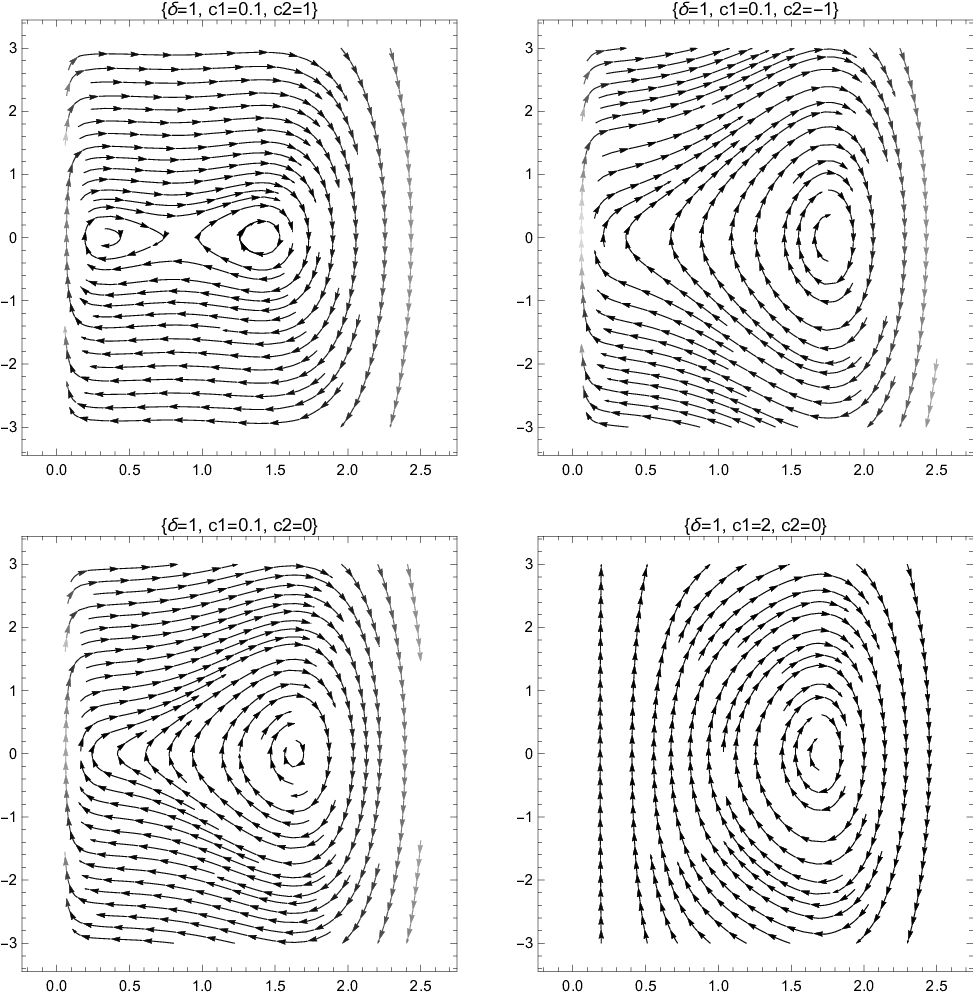
In Fig. 1 we present the phase portrait of equation (14) from where it is clear that there are attractors in the dynamical system which provide a periodic behaviour.

Refer to caption — Figure 1: Phase portrait for equation (14) for various values of the free parameters $\left\{\delta,c_{1},C_{2}\right\}$ .

In order to write the analytic solution of equation (14) and understand the periodic behaviour of the solution, we apply the singularity analysis. Specifically we apply the ARS algorithm. We search for the singular behaviour $\varrho\left(x\right)=\varrho_{0}x^{p}$ from where we follows that the leading-order behaviour has $p=-\frac{1}{2}$ and $\left(\varrho_{0}\right)^{2}=\pm\frac{i}{\delta},$ it is clear from here that a periodic behaviour will follow.

The second step of the ARS algorithms is the determination of the resonances, we do that by replacing $\varrho\left(x\right)=\varrho_{0}x^{-\frac{1}{2}}+mx^{-\frac{1}{2}+S}$ in (14) and linearize around $m=0$ , it follows the algebraic equation $\left(S+1\right)\left(S-3\right)=0$ , which gives the resonances $S=-1$ and $S=3$ .

Finally we write the Laurent expansion

\varrho\left(x\right)=\varrho_{0}x^{-\frac{1}{2}}+\varrho_{1}x^{\frac{1}{2}}+\varrho_{2}x^{\frac{3}{2}}+...~,

(16)

from where we test that it is a solution of equation (12) with integration constant the $\varrho_{3}$ and

\left(\varrho_{0}\right)^{2}=\pm\frac{i}{\delta}~,~\varrho_{1}=-\frac{\left(-1\right)^{\frac{3}{4}}}{2\delta^{\frac{3}{2}}}~,~\varrho_{2}=-\frac{\left(-1\right)^{1/4}\left(9-8\bar{C}_{2}\delta\right)}{24\delta^{\frac{5}{2}}},~...~.

We remark that the second integration constant is the position of the singularity $x_{0}$ .

2.1.2 Lie symmetry $X_{2}$

Reduction with respect to the vector field $X_{2}$ provides the stationary solutions $u=u\left(t\right),~\rho=\rho\left(t\right)$ where $u_{t}=0$ and $\rho_{t}=0$ , that is $u\left(t,x\right)=u_{0},~\rho\left(t,x\right)=u_{0}$ .

2.1.3 Lie symmetry $X_{1}+\alpha X_{2}$

The application of the Lie symmetry vector $X_{1}+\alpha X_{2}$ provides a travel-wave solution. Indeed we find $u=u\left(z\right),~\rho=\varrho^{2}\left(z\right)$ with $z=x-\alpha t$ , where now the reduced system is

\left(u-\alpha\right)\varrho^{2}+\frac{1}{2}\delta\varrho^{4}=c_{1}~,

(17)

\varrho_{zz}+2\left(\alpha-\delta\varrho^{2}\right)\rho u-u^{2}\varrho-\varrho^{3}+c_{2}\varrho=0~,

(18)

where $c_{1},~c_{2}$ are two integration constants.

With the use of (17), equation (18) reads as

\varrho_{zz}+\frac{3}{4}\delta^{2}\varrho^{5}-2\left(1+\alpha\delta\right)\varrho^{3}+\bar{C}_{2}\varrho-\frac{c_{1}^{2}}{\varrho^{3}}=0~,

(19)

with $\bar{C}_{2}=\left(c_{2}-\alpha-\delta c_{1}\right)$ .

Equation (19) is of the form of the static solution (14) and can be integrated by quadratures, the only main difference is the coefficient of the $\varrho^{3}$ , where now it is $\left(1+\alpha\delta\right)$ . The latter quantity can be positive or negative, either if the travel wave travel of the left to the right or from the right to the left.

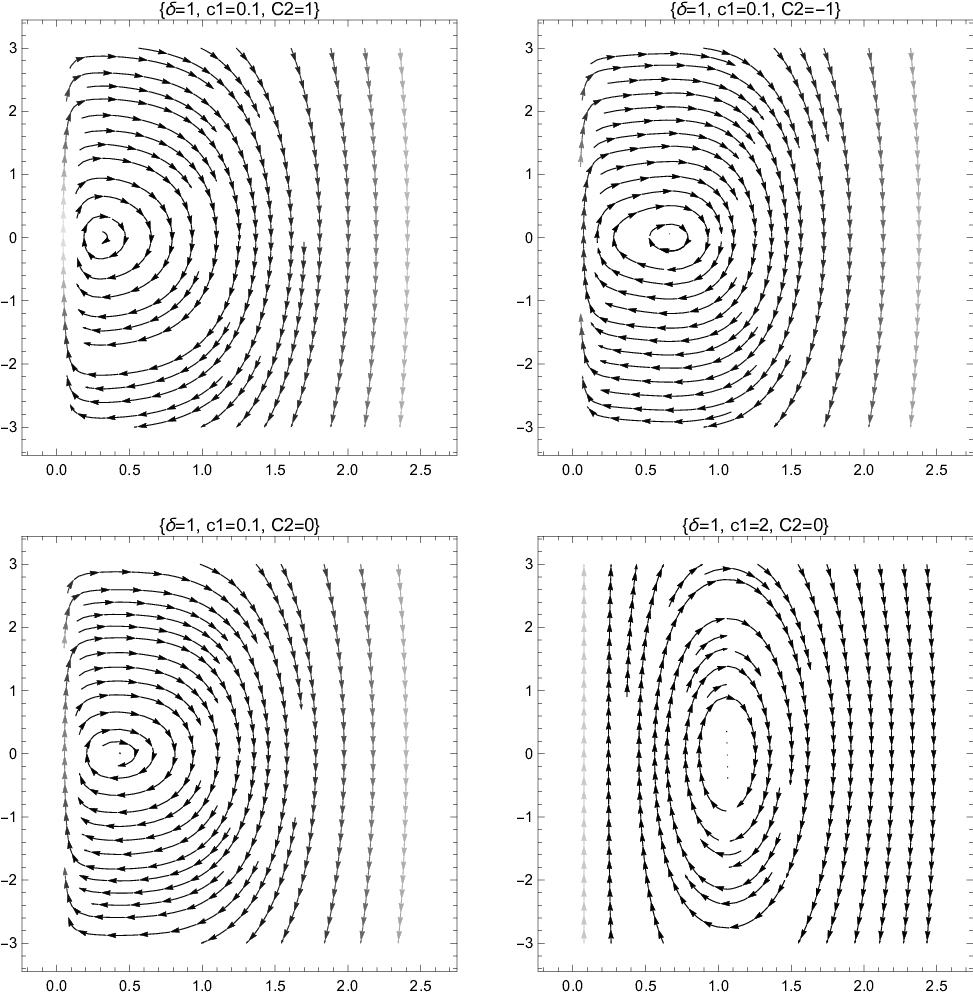
In Fig. 2 we present the phase portrait for the equation (19) and $\left(1+\alpha\delta\right)<0,$ specifically for $\left(1+\alpha\delta\right)=-1$ , and for the rest of the constants to have the same values as in Fig. 1. Again we observe a similar behaviour and the existence of periodic solutions which correspond to travel-wave solutions.

As in the case of the static solution, the application of the singularity analysis provides the analytic solution expressed by the Laurent expansion

\varrho\left(x\right)=\varrho_{0}x^{-\frac{1}{2}}+\varrho_{1}x^{\frac{1}{2}}+\varrho_{2}x^{\frac{3}{2}}+...~,

(20)

where now

\left(\varrho_{0}\right)^{2}=\pm\frac{i}{\delta}~,~\varrho_{1}=-\frac{\left(-1\right)^{\frac{3}{4}}}{2\delta^{\frac{3}{2}}}\left(1+\alpha\delta\right)~,~\varrho_{2}=-\frac{\left(-1\right)^{1/4}\left(9\left(1+\alpha\delta\right)^{2}-8\bar{C}_{2}\delta\right)}{24\delta^{\frac{5}{2}}},~...~.

(21)

and $\varrho_{3}$ is an arbitrary constant.

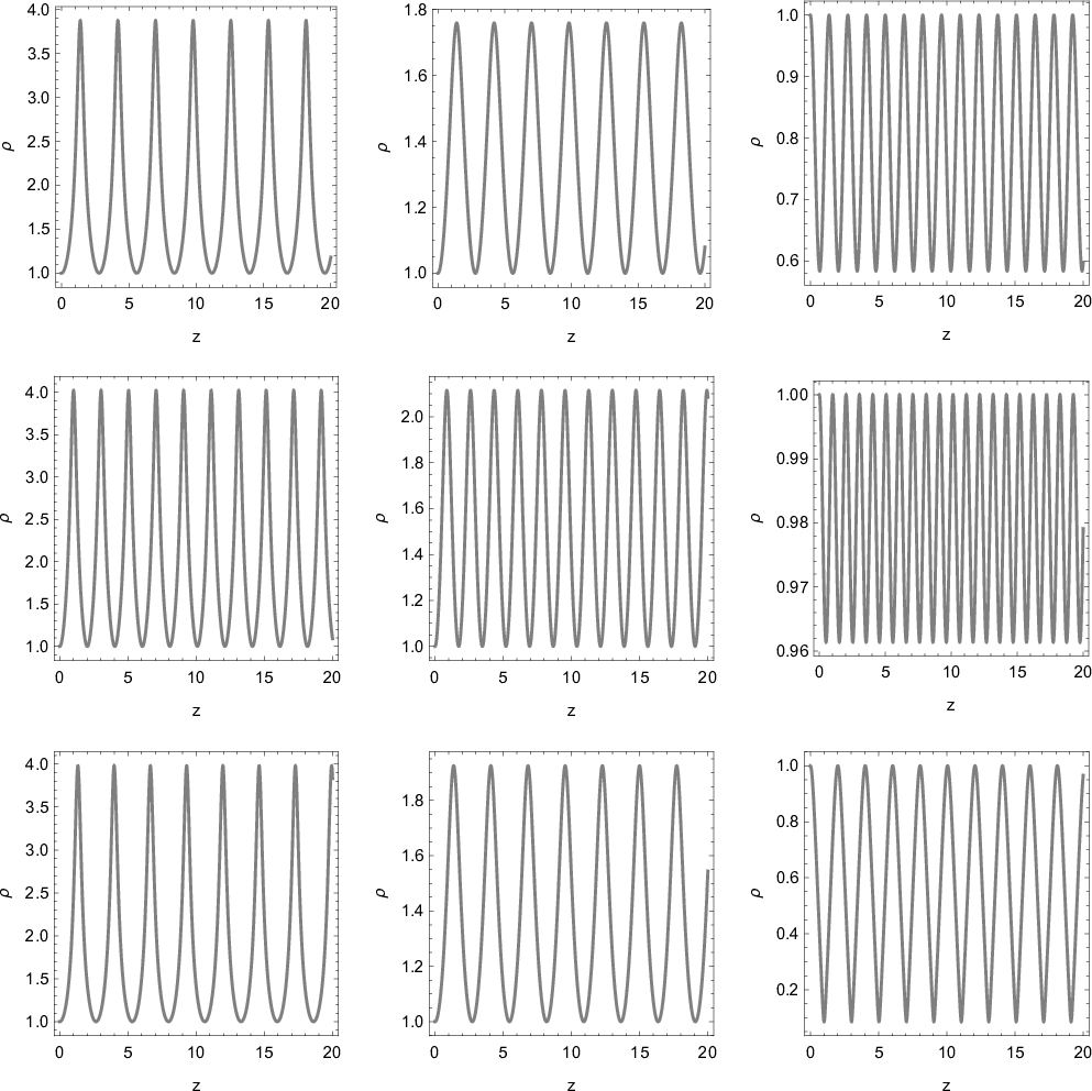
In Fig. 3 we present the numerical solution of (19) where we observe the existence of travel-waves, i.e. a kink solutions, for the gCLL equation.

2.1.4 Lie symmetry $X_{3}$

We proceed with the application of the similarity transformation provided by the scaling symmetry $X_{3}$ . The similarity transformation is

u\left(t,x\right)=-\frac{1}{\delta}+\frac{1}{\sqrt{t}}U\left(\sigma\right)~,~\rho\left(t,x\right)=\frac{1}{\sqrt{t}}R^{2}\left(\sigma\right)~\text{with}~\sigma=\left(\frac{x}{\sqrt{t}}+\frac{\sqrt{t}}{\delta}\right)\text{.}

(22)

Therefore, the reduced system after the application of the latter similarity transformation is derived to be

2RU-\sigma R+\delta R^{2}=c_{1},

(23)

R_{\sigma\sigma}-U^{2}R+\left(\sigma-2\delta R^{2}\right)UR+c_{2}R=0,

(24)

where $c_{1},~c_{2}$ are two integration constants.

Therefore, we end with only one differential equation

R_{\sigma\sigma}+\frac{3}{4}\delta^{2}R^{5}-2\left(1+\alpha\delta\right)R^{3}+\left(C_{2}+\frac{\sigma^{2}}{4}\right)R-\frac{c_{1}^{2}}{R^{3}}=0

(25)

where now $C_{2}=\left(\frac{c_{2}}{2}-\delta c_{1}\right)$ . The main difference with the previous reduction is that the coefficient of the linear term is not a constant.

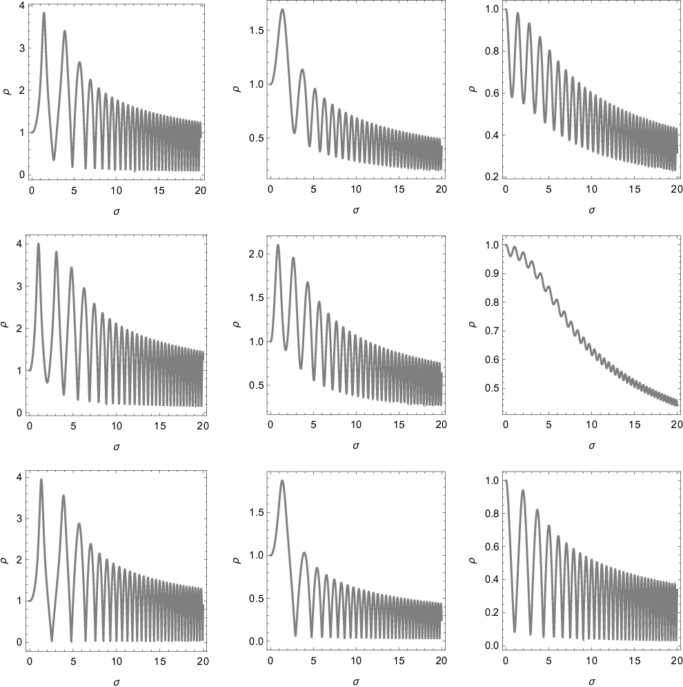
Easily, we observe that the resulting solution is again periodic solution but in this case around a central which moves. In Fig. 4 we present numerical simulation for equation (25) for the initial condition $R\left(0\right)=1~,~R_{\sigma}\left(0\right)=0\,\$ and for various values of the free parameters $\left\{c_{1},C_{2},\left(1+\alpha\delta\right)\right\}$ , from the figures it is clear the periodic behaviour of the scaling solution, that is nothing else than a kink solution.

For small values of $R$ , the dominant terms are the

R_{\sigma\sigma}+\left(C_{2}+\frac{\sigma^{2}}{4}\right)R-\frac{c_{1}^{2}}{R^{3}}=0

(26)

which is nothing else than the Ermakov-Pinney equation [58, 59, 60].

3 Singularity analysis

Let us now apply the ARS algorithm to study if the system (2), (3) possess the Painlevé property.

In order to determine the singular behaviour we replace in (2), (3) the following expression

\rho\left(t,x\right)=\rho_{0}\left(t,x\right)\phi\left(t,x\right)^{p}~,~u\left(t,x\right)=u_{0}\left(t,x\right)\phi\left(t,x\right)^{q}

where $\phi\left(t,x\right)$ is a singular function. Hence, it follows that the leading order terms provide $\left\{p,q\right\}=\left(-1,-1\right)$ , where

\rho_{0}\left(t,x\right)=-\frac{1}{\delta^{2}}\phi_{x}^{2}~,~u_{0}\left(t,x\right)=-\frac{1}{4}\phi_{x}^{2}\text{.}

For the second step of the ARS algorithm, we determine the resonances which are $\left\{s_{1},s_{2},s_{3},s_{4}\right\}=\left\{-1,2,2,3\right\}$ from where we conclude that the solution is given by Right Painlevé Series. Indeed the solutions is expressed as

\rho\left(t,x\right)=\rho_{0}\left(t,x\right)\phi\left(t,x\right)^{-1}+\rho_{1}\left(t,x\right)+\rho_{2}\left(t,x\right)\phi\left(t,x\right)+\rho_{3}\left(t,x\right)\phi\left(t,x\right)^{3}+...~,

(27)

u\left(t,x\right)=u_{0}\left(t,x\right)\phi\left(t,x\right)^{-1}+u_{1}\left(t,x\right)+u_{2}\left(t,x\right)\phi\left(t,x\right)+u_{3}\left(t,x\right)\phi\left(t,x\right)^{3}+...~.

(28)

where the consistency test gives that functions $\rho_{2}\left(t,x\right),~\rho_{3}\left(t,x\right)$ and $u_{2}\left(t,x\right)$ are arbitrary.

We conclude that the generalized Chen-Lee-Liu equation possess the Painlevé property and its solution is expressed by Right Laurent expansions. The latter expressions can describe Kink solutions for specific initial conditions.

4 Conclusion

In this work we determined exact and analytic periodic solutions for the gCLL equation with the use of Lie symmetries. The gCLL equation admits a three-dimensional Lie algebra, which leads to four different similarity transformations. In particular we found static, stationary, travel-wave and scaling similarity solutions.

Except from the stationary solution, which is not of interest, the other solutions are periodic solutions. It is interesting that in all cases for small values of the intensity variable $\rho\left(t,x\right)$ the gCLL is reduced to the Ermakov-Pinney equation, which is a well-known integrable system.

Moreover, we investigated if the gCLL possess the Painlevé property, for that we applied the ARS algorithm where we were able to write the analytic solution of the gCLL with the use of Right Painlevé Series.

The periodic solutions, provided by the similarity transformations, are direct related with the existence of dark and bright solitons for the nonlinear differential equation [61, 62, 63]. Optical solitons are exact solutions of mathematical models with direct applications in the information transfer in optical fibers [64]. As far the results or our analysis, are concerned, the travel-wave solution which was found before for the gCLL describes a 1-soliton solution known as kink solution. Furthermore, the scaling solution is also a kink solution, where now the amplitude of the oscillation is not a constant.

The determination of these new kink solutions is essential for the physical viability of the model. A study of the properties of the kink solutions and their real world applications extends the scopus of this study and will be performed in a future study.

Appendix A Lie symmetries

We briefly discuss the main definition and algorithm for the determination of Lie point symmetries. Consider the one-dimensional parameter point transformation

	$\displaystyle\bar{x}^{k}$	$\displaystyle=x^{k}+\epsilon\xi^{i}\left(x^{k},u\right),$		(29)
	$\displaystyle\bar{\eta}$	$\displaystyle=\eta+\epsilon\eta\left(x^{k},u\right).$		(30)

with generator $X=\xi^{i}\left(x^{k},u\right)\partial_{i}+\eta\left(x^{k},u\right)\partial_{u}$ , then the differential equation $\mathbf{H}\left(x^{k},u,u_{i},u_{ij},...,u_{i_{1}i_{2}...i_{n}}\right)$ is invariant under the action of the one parameter point transformation if and only if

\lim_{\varepsilon\rightarrow 0}\frac{\mathbf{\bar{H}}\left(\bar{x}^{k},\bar{u},\bar{u}_{i},\bar{u}_{ij},...,\bar{u}_{i_{1}i_{2}...i_{n}}\right)-\mathbf{H}\left(x^{k},u,u_{i},u_{ij},...,u_{i_{1}i_{2}...i_{n}}\right)}{\varepsilon}=0,

or equivalently, if there exists a function $\lambda$ such that the following condition to be true [4, 1, 2]

X^{\left[n\right]}\mathbf{H}-\lambda\mathbf{H=0}

(31)

where $X^{\left[n\right]}$ is called the n-th prolongation/extension of $X~$ in the jet-space defined as

X^{\left[n\right]}=X+\left(D_{i}\eta-u_{,k}D_{i}\xi^{k}\right)\partial_{u_{i}}+\left(D_{i}\eta_{j}^{\left[i\right]}-u_{jk}D_{i}\xi^{k}\right)\partial_{u_{ij}}+...+\left(D_{i}\eta_{i_{1}i_{2}...i_{n-1}}^{\left[i\right]}-u_{i_{1}i_{2}...k}D_{i_{n}}\xi^{k}\right)\partial_{u_{i_{1}i_{2}...i_{n}}}.

(32)

If $X$ is a symmetry vector for the differential equation $\mathbf{H}$ , then we can always find a coordinate transformation such that the symmetry vector to be written in the canonical coordinates, i.e. $X=\partial_{x^{n}}$ , where the differential equation is

\mathbf{H=H}\left(x^{\mu},u,u_{i},u_{ij},...,u_{i_{1}i_{2}...i_{n}}\right)~,~\mu\neq n,

clear from the last expression it follows $\partial_{x^{\mu}}H=0$ . The coordinate transformation which leads to the canonical coordinates it is called similarity transformation and it is mainly applied for the reduction of the differential equation,

Appendix B One-dimensional optimal system

Let a given differential equation admit as Lie symmetries the elements $\left\{X_{1},~X_{2},~...~X_{n}\right\}$ of the $n$ -dimensional Lie algebra $G_{n}$ with structure constants $C_{jk}^{i}$ . The two symmetry vectors $Z,~W$ defined as

Z=\sum_{i=1}^{n}a_{i}X_{i}~,~W=\sum_{i=1}^{n}b_{i}X_{i}~,~\text{\ }a_{i},~b_{i}\text{ are constants.}

(33)

we shall say that are equivalent if and only if [3]

\mathbf{W}=\sum_{j=i}^{n}Ad\left(\exp\left(\epsilon_{i}X_{i}\right)\right)\mathbf{Z}

(34)

W=cZ~,~c=const\text{ that is }b_{i}=ca_{i}\text{.}

(35)

Operator $Ad\left(\exp\left(\epsilon X_{i}\right)\right)X_{j}$ defined as

Ad\left(\exp\left(\epsilon X_{i}\right)\right)X_{j}=X_{j}-\epsilon\left[X_{i},X_{j}\right]+\frac{1}{2}\epsilon^{2}\left[X_{i},\left[X_{i},X_{j}\right]\right]+...,

(36)

is called the adjoint representation.

The determination of all the one-dimensional subalgebras of $G_{n}$ which are not related through the adjoint representation it is necessary in order to perform a complete classification of all the possible similarity transformations, i.e. similarity solutions, for a given differential equation. This classification is known as the one-dimensional optimal system.

Appendix C Singularity analysis

The development of the Painlevé Test for the determination of integrability of a given equation or system of equations and its systematization been succinctly summarized by Ablowitz, Ramani and Segur in the so-called ARS algorithm [53, 54, 55]. The ARS algorithm is constructed by three basic steps, they are: (a) determine the leading-order term which describes the behaviour of the solution near the singularity, (b) find the position of the resonances which shows the existence and the position of the integration constants and (c) write a Laurent expansion with leading-order term determined in the first step in order to perform the consistency test and the solution, for a review on the ARS algorithm and various applications we refer the reader in [56], while in [57] a discussion between the Lie’s approach and the singularity analysis is given.

References

[1] G.W. Bluman and S. Kumei, Symmetries of Differential Equations, Springer-Verlag, New York, (1989)
[2] H. Stephani, Differential Equations: Their Solutions Using Symmetry, Cambridge University Press, New York, (1989)
[3] P.J. Olver, Applications of Lie Groups to Differential Equations, Springer-Verlag, New York, (1993)
[4] N.H. Ibragimov, CRC Handbook of Lie Group Analysis of Differential Equations, Volume I: Symmetries, Exact Solutions, and Conservation Laws, CRS Press LLC, Florida (2000)
[5] L. V. Ovsiannikov, Group analysis of differential equations, Academic Press, New York, (1982)
[6] F.M. Mahomed and A. Qadir, J. Nonlinear Math. Phys. 16, 283 (2009)
[7] H.M. Dutt, M. Safdar and A. Qadir, Arabian Journal of Mathematics 8, 163 (2019)
[8] M. Ayub, M. Khan and F.M. Mahomed, Nonlinear Dynamics 67, 2053 (2012)
[9] W. Rui and X. Zhang, Comm. Nonl. Sci. Num. Sim. 34, 38 (2016)
[10] W. Sarlet and F. Cantrijin, SIAM Review 23, 467 (1981)
[11] S.A. Hojman, J. Math. Phys. A: Math. Gen. 24, L291 (1992)
[12] P.J. Olver and P. Rosenau, SIAM J. Appl. Math. 47, 263 (1987)
[13] G.M. Webb and G.P. Zank, J. Math. Phys. A: Math. Theor. 40, 545 (2007)
[14] M.T. Mustafa, A.Y. Al-Dweik and R.A. Mara’beh, SIGMA 9, 041 (2013)
[15] P.G.L. Leach, J. Math. Phys. 26, 510 (1985)
[16] A. Paliathanasis and M. Tsamparlis, Int. J. Geom. Meth. Mod. Phys. 11, 1450037 (2014)
[17] S.V. Meleshko and V.P. Shapeev, J. Nonl. Math. Phys. 18, 195 (2011)
[18] G.M. Webb, J. Phys A: Math. Gen. 23, 3885 (1990)
[19] C.M. Khalique and A. Biswas, Comm. Non. Sci. Num. Sim. 14, 4033 (2009)
[20] L. Gagnon, B. Grammaticos, A. Ramani and P. Winternitz, J. Phys. A.: Math. Gen. 22, 499 (1989)
[21] W.I. Fushchych and A.G. Nikitin, J. Math. Phys. 38, 5944 (1997)
[22] X.X. Du, B. Tian, Y.-Q. Yuan and Z. Du, Annalen de Physik 531, 1900198 (2019)
[23] Y. Benia, M. Ruggieri and A. Scapellato, Mathematics, 7, 908 (2019)
[24] X. Xin, H. Liu, L. Zhang and Z. Wang, Appl. Math. Lett. 88, 132 (2019)
[25] M. Pandey, Int. J. Nonl. Sci. Num. Sim. 16, 93 (2015)
[26] J.-G. Liu, Z.-F. Zeng, Y. He and G.-P. Ai, Int. J. Nonl. Sci. Num. Sim. 16, 114 (2013)
[27] P. Painlevé, Bulletin of the Mathematical Society of France 28 201 (1900)
[28] P. Painlevé, Acta Mathematica 25, 1 (1902)
[29] P. Painlevé, Comptes Rendus de la Académie des Sciences de Paris 143, 1111 (1906)
[30] S. Kowalevski, Acta. Math. 12, 177 (1889)
[31] T. Brugarino and M. Sciacca, Optics Commun. 262, 250 (2006)
[32] K. Andriopoulos and P.G.L. Leach, J. Math. Anal. Appl. 328, 860 (2007)
[33] K. Andriopoulos and P.G.L. Leach, Appl. Anal. Disc. Math. 5, 230 (2011)
[34] A. Paliathanasis, J.D. Barrow and P.G.L. Leach, Phys. Rev. D 94, 023525 (2016)
[35] R. Conte, Phys. Lett. A, 134, 100 (1988)
[36] R. Conte, Phys. Lett. A, 140, 383 (1989)
[37] M. Vlieg-Hulstman, Mathl. Comput. Modelling 18, 151 (1993)
[38] S.K. Ivanov, Phys. Rev. A 101, 053827 (2020)
[39] C. Rogers and K.W. Chow, Phys. Rev. E 86, 037601 (2012)
[40] W.H. Lin and E. Kenghe, Schrodinger equations in nonlinear systems, Springer Nature, Singapore, (2019)
[41] A. Hussain, A. Jhangeer, S. Tahir, Y.-M. Chu, I. Khan and K.S. Nisar, Results in Physics 18, 103208 (2020)
[42] M. Bilal, W. Hu and J. Ren, Eur. Phys. J. Plus 136, 385 (2021)
[43] O. Gonzalez-Gaxiola and A. Biswas, Optical and Quantum Electronics 50, 314 (2018)
[44] G. Xu, M. Confroti, A. Kudlinski, A. Mussot and S. Trillo, Phys. Rev. Lett. 118, 254101 (2017)
[45] K.B. Wolf, Annals of Physics, 172, 1 (1986)
[46] A. Bansal, A. Biswas, A.S. Alshomrani, M. Ekici, Q. Zhou and M.R. Belic, Results in Physics 15, 102713 (2019)
[47] C.M. Khalique and A. Biswas, J. Electromagnetic Waves and Appl. 23, 963 (2009)
[48] A. Bansal, A. Biswas, Q. Zhou, S. Arshed, A.K. Alzahrani and M.R. Belic, Phys. Lett. A 384, 126202 (2020)
[49] V.V. Morozov, Izvestia Vysshikh Uchebn Zavendeniĭ Matematika, 5 161-171 (1958)
[50] G.M. Mubarakzyanov, Izvestia Vysshikh Uchebn Zavendeniĭ Matematika, 32 114-123 (1963)
[51] G.M. Mubarakzyanov, Izvestia Vysshikh Uchebn Zavendeniĭ Matematika, 34 99-106 (1963)
[52] G.M. Mubarakzyanov, Izvestia Vysshikh Uchebn Zavendeniĭ Matematika, 35 104-116 (1963)
[53] M.J. Ablowitz, A. Ramani and H. Segur, Lettere al Nuovo Cimento 23, 333 (1978)
[54] M.J. Ablowitz, A. Ramani and H. Segur, J. Math. Phys. 21, 715 (1980)
[55] M.J. Ablowitz, A. Ramani and H. Segur, J. Math. Phys. 21, 1006 (1980)
[56] A. Ramani, B. Grammaticos and T. Bountis, Phys. Rept. 180, 159 (1989)
[57] A. Paliathanasis and P.G.L. Leach, IJGMMP 13, 1630009 (2016)
[58] J. Ray and J.L. Reid, Phys. Lett. A 71, 317 (1979)
[59] E. Pinney, Proc. Am. Math. Soc. 1, 681 (1950) erm2,erm3,erm4
[60] S. Moyo and P.G.L. Leach, J. Phys. A: Math. and Gen. 35, 5333 (2002)
[61] A.S.H.F. Mahomed and H.O. Bakodah, Phys. Scr. 96, 035206 (2021)
[62] H. Triki, M.M. Babatin and A. Biswas, Optik 149, 300 (2017)
[63] Z. Xu, L. Li, Z. Li and G. Zhou, Phys. Rev. E 67, 026603 (2003)
[64] A. Hasegawa and M. Matsumoto, Optical Solitons in Fibres, Springer Series in Photonics, Springer-Verlag Berlin Heidelberg (2003)