Singularities in static spherically symmetric configurations of General Relativity with strongly nonlinear scalar fields
Abstract
There are a number of publications on relativistic objects dealing either with black holes or naked singularities in the center. Here we show that there exist static spherically symmetric solutions of Einstein equations with a strongly nonlinear scalar field with potential , which allow the appearance of singularities of a new type (“spherical singularities”) outside the center of isolated configuration. The space-time is assumed to be asymptotically flat. Depending on the configuration parameters, we show that the distribution of the stable circular orbits of test bodies around the configuration is either similar to that in the case of the Schwarzschild solution (thus mimicking an ordinary black hole), or it contains additional rings of unstable orbits.
Keywords:
naked singularities, test particle motion, accretion diskspacs
11I Introduction
Nowadays, the concept of a black hole has become a common element of astrophysical research Novikov and Thorne 1973; Antonucci 1993; Bianchi et al. 2012. However, in order to be fully confident in the theoretical idea, it must be compared with alternative models. This is one of the motivations for many theoretical works devoted to non-canonical and even exotic solutions of General Relativity and its modifications, which could have similar astrophysical consequences. The non-exhaustive list below includes papers on various aspects of compact objects with naked singularities Stuchlík and Schee 2014; Shao et al. 2021; Chakraborty and Bhattacharyya 2019; Bhattacharya et al. 2020; Pugliese et al. 2011; Pugliese et al. 2013; Joshi et al. 2013; Shahidi et al. 2020; Boshkayev et al. 2016; Stashko and Zhdanov 2018; Bambhaniya et al. 2019, with wormholes Karimov et al. 2019; Paul et al. 2019; Narzilloev et al. 2021; Abdujabbarov and Ahmedov 2009; Li and Bambi 2014, boson stars Vincent et al. 2016; Grandclément et al. 2014; Liebling and Palenzuela 2017; Lamy et al. 2018; Herdeiro et al. 2021, and the other non-singular objects mimicking the black holes Dymnikova and Poszwa 2019; Stuchlík and Schee 2015; Schönenbach et al. 2014. The question arises as to how the aforementioned exotic configurations were formed; probably, not all corresponding models can reflect real astrophysical situations. However, final answers about the reality of these models must be based on observations. This explains why the interest in the “black hole mimickers” greatly increased after the Event Horizon Telescope observed the image of the accretion disk around the supermassive black hole in the center of M87 Collaboration 2019. Correspondingly, much attention is paid to the observational manifestations of different models dealing with motion of test particles and photons in the gravitational field of the compact object Chowdhury et al. 2012; Stuchlík and Schee 2014; Stuchlík and Schee 2015; Zhou et al. 2015; Chakraborty and Bhattacharyya 2019; Dymnikova and Poszwa 2019; an important point concerns the images of accretion disks, radiation fluxes, forms of the relativistic Fe line Shaikh and Joshi 2019; Gyulchev et al. 2019; Gyulchev et al. 2020; Gyulchev et al. 2021; Collodel et al. 2021; Sau et al. 2020; Schönenbach et al. 2014; Cao et al. 2016; Yang et al. 2018; Shen et al. 2017; Liu et al. 2018, etc.
A number of models are based on static solutions of the Einstein equations with scalar field (SF) Chowdhury et al. 2012; Zhou et al. 2015; Shaikh and Joshi 2019; Gyulchev et al. 2019; Gyulchev et al. 2020; Martínez et al. 2004; Sau et al. 2020. These papers use analytically defined metrics, in particular the Fisher–Yanis–Newman–Winicour solution Fisher 1948; Janis et al. 1968; Wyman 1981; Virbhadra 1997. Papers Sau et al. 2020; Shaikh and Joshi 2019; Gyulchev et al. 2019; Gyulchev et al. 2020; Chowdhury et al. 2012; Zhou et al. 2015 deal with singularities in the center, the solutions used do not have other “physical” singularities outside the center. It was proved Zhdanov and Stashko 2020 that this is a fairly general situation, at least when considering an isolated spherically symmetric configuration of General Relativity with a scalar field. Here the gravitational field suppresses the appearance of “spherical singularities” and only a naked singularity in the very center is possible. The proof uses an assumption that the SF self-interaction potential is exponentially bounded Zhdanov and Stashko 2020. Thus, the singularity for any non-zero value of the radial variable in the curvature (Schwarzschild) coordinates is prohibited and the question arises whether this result will be preserved in the case of a sharper dependence of the SF potential for the large field values? This is a key point of the present paper.
In this article, our goal is to provide examples showing that in the case of a sufficiently strong nonlinear behavior of the potential (with a sufficiently fast growth rate), spherical singularities (SS) can arise. To relax the restrictions of Zhdanov and Stashko 2020, we choose , as a representative of such potentials. This is a technically convenient choice: for large , this potential grows faster than any exponentially bounded function; on the other hand, for small it behaves as a monomial potential that allows us to use earlier results concerning asymptotic behavior for .
The paper is organized as follows. In Section II we present initial relations. In Sections III and IV we show the possibility of “spherical singularities” and present numerical solutions for the Einstein equations with SF in the case of spherical symmetry. In Section V we study distributions of the stable circular orbits (SCO), which is important to study a thin accretion disk around the configuration. We also estimate the radiation flux from the accretion disk within the Page–Thorne model Page and Thorne 1974.
II Initial Relations
We consider a static spherically symmetric space-time metric in the curvature coordinates, that is
| (1) |
this fixes the radial variable .
The gravitational field interacts with real SF described by Lagrangian density
| (2) |
the SF potential is
| (3) |
This potential is strongly nonlinear for and for it grows faster than for any .
The SF equation following from (2) is
| (4) |
The independent from (4) Einstein equations are reduced to the form (see, e.g., Zhdanov and Stashko 2020)
| (5) |
| (6) |
We focus on isolated systems with mass in the asymptotically flat space-time assuming for
| (7) |
As for SF, we assume ; then for (3) we have for and therefore we can use some of the results on monomial potentials from Zhdanov and Stashko 2020; Stashko et al. 2021, concerning asymptotic behavior for large :
for (linear massive scalar field with mass Stashko and Zhdanov 2019);
| (8) |
(see Appendix A of Zhdanov and Stashko 2020); asymptotic relations for can be obtained by formal differentiation of (8).
III Asymptotic Behavior Near Singularity
First of all we note that for regular solutions of (4)–(6) within some interval , satisfying conditions (8) with non-trivial , we can show that functions and preserve their signs. Indeed, for potential (3) inequality is valid for , and using Equation (4) we get
| (9) |
Therefore, function is monotonically increasing. On account of conditions (7) and (8), it is strictly negative for large ; therefore it cannot be equal to zero and so is . Whence we infer that functions do not change their signs.
Further, for definiteness, we assume , .
Now we turn to the singularities at some in case of potential (3). We are looking for solutions on such that
| (10) |
for some . Our aim is to estimate asymptotic properties of these solutions.
Numerical simulations near singularity suggests that is a slowly varying function. So, as a first approximation, we are neglecting this function compared to . Under this assumption we get for the leading terms of Equation (4)
| (12) |
This is a rough approximation that is valid in very small interval near the singularity. We have then , where the constant will be neglected in comparison with for , so that
| (13) |
In view of (10), for and then it is easy to see that the principal terms on the right hand sides of (5) and (6) are asymptotically the same. This justifies our assumption about .
Substitution into (11) yields
| (14) |
where we discarded the lower order terms. This allows us to reduce the problem to the system of two equations .
Then is monotonically increasing (for , where ). For Equation (14) yields
| (15) |
From Equation (13) we have
| (16) |
where we take into account that is decreasing.
Dividing (15) by (16) we have equation
that can be solved in quadratures. In the leading terms for
| (17) |
where we denote
This can be expressed by the incomplete gamma-function, leading to the asymptotic formula:
| (18) |
The solution is
The limit (10) occurs if
| (19) |
Then
| (20) |
Using (17) we have
| (21) |
The Kretschmann invariant near has the form
| (22) |
The main outcome of these considerations is that there exist singularities of solutions to systems (4)–(6) for some non-zero value of the radial variable in curvature coordinates, that is, SS are indeed possible. This does not mean that all the solutions have such singularities. It easy to see that for to have the singularity at some , the condition (19) must be fulfilled (i.e., must be sufficiently large). The latter depends on the initial conditions at infinity and this must be derived numerically. This is a subject of the next section.
IV Numerical Solutions
Here we restrict ourselves to the case of a long-range field . Correspondingly, taking into account (8), we assume the conditions for the field
| (23) |
yielding
| (24) |
It was shown in Stashko et al. 2021 that there is a unique solution of the problem for sufficiently large satisfying (4)–(6) and (24). The iteration procedure yielding the solution is described in Stashko et al. 2021 for a monomial potential and it can be applied in case of (3) for sufficiently large (small ). This yields initial conditions for the ordinary differential system (4)–(6) at some (large) . Instead, one can directly use asymptotic expansions to derive the solution for large . We obtained the solution numerically by integrating the equations backward from to smaller values of , either to a spherical singularity or to a point-like naked singularity at the origin. The occurrence of singularity can be checked by means of relation (19); this can be used in order to define more precisely the singularity radius.
Figures 1 and 2 show typical behavior of solutions in the case of SS; we see that is monotonically increasing, whereas reaches a maximum and then decreases to one for . Additionally, we note that near the singularity for in accordance with Section III. Figures 3–5 show a non-trivial dependence of the singularity radii upon parameters .


V Test Particle Motion
In this section, we consider the massive test particles motion around static spherically symmetric configurations with SF to describe in order to describe characteristics of accretion onto a singularity. We use the Page–Thorne model Page and Thorne 1974 of a thin accretion disk (AD). In this model, the averaged motion of the accreting matter is essentially described by SCOD in the equatorial plane.
In the case of spherically symmetric space-time with metric (1), the standard procedure yields the first integrals for test particle trajectories in the equatorial plane ( is a canonical parameter.):
| (25) |
| (26) |
where in case of null trajectories and for the test particles with the non-zero mass; are the integrals of motion. This yields
| (27) |
where effective potential .
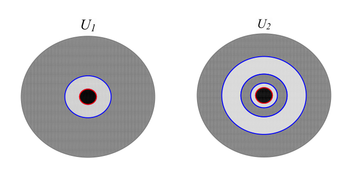
The form of , in particular, the disposition of its minima and maxima, defines the distribution of stable circular orbits (SCO) and unstable ones. The SCO distribution (SCOD) is the most important because it forms the basis for evaluating the properties of an accretion disc around the configuration described by Equations (4)–(6). Possible types of SCODs are listed in Table 1 and described schematically on Figure 6.
| Type | Photon sphere | ||
|---|---|---|---|
We use a method of our works Stashko and Zhdanov 2018; Stashko and Zhdanov 2019 to study bifurcations associated with the appearance and disappearance of the minima of . Figure 7 illustrates how the shape of the effective potential changes with an increase in in case of the SCOD type. Essentially this is connected with investigation of joint conditions and , which allow us to exclude ; this leads to a necessary condition , where
| (28) |
For the congruence of circular orbits with different radii in equatorial plane we get dependencies of the specific energy and the specific angular momentum, and the angular velocity upon radius as follows
| (29) |
Using Equation (28), we numerically get the bifurcation values and under conditions that and . This allows us to determine SCOD types for given configuration parameters. Figure 8 shows the corresponding results in the plane. Also, Figure 9 illustrates the dependence of the boundary radii (i.e., radii of the blue circles in Figure 6) upon and .


Now we consider radiation from the stationary thin AD described by Page–Thorne model Page and Thorne 1974. The time averaged radiation flux from the surface of the accretion with inner edge located at the boundary SCO is
| (30) |
where is the metric’s determinant in the equatorial plane and is the mass accretion rate that is assumed to be constant. Specific particle energy, momentum, and angular velocity are defined from (29). We obtained the radiation flux for several values in presence/absence of inner stable ring of AD. The corresponding fluxes are shown in Figure 10. To compare different types, we normalize them to the maximum flux in the case of a Schwarzschild black hole . We see that the maximum value of different types can be less or more then as distinct from the case of the massless scalar field Chowdhury et al. 2012; Gyulchev et al. 2020, where due to .


VI Discussion
We have shown that General Relativity allows the existence of SS in static spherically symmetric configurations in the case of the SF potential , which represents potentials with fast growth rate. This statement follows from the analytical reasoning of Section III and is confirmed by numerical simulations of Section IV. These SS are “physical” singularities that cannot be removed by a coordinate transformation: this can be seen from the behavior of the Kretschmann invariant. These are naked singularities, because they can be observed by a distant observer; it is easy to verify this by considering the radial motion of photons, taking into account that near the singularity for .
We note that the appearance of singularities in solutions of nonlinear equations is a fairly typical case. However, the situation with SS is different from the case of monomial or the other exponentially bounded potentials, when SS are suppressed by the gravitational field and we only have a naked singularity at the center Zhdanov and Stashko 2020. In the case of , the sharp growth of the field near the singularity overcomes this suppression. This suggests that SS can occur for more general potentials with fairly rapid growth.
Having the numerical solutions, we investigated the location of stable and unstable circular orbits. There are two main types of SCOD in our case: (i) is similar to SCOD in the case of the Schwarzschild metric, when SCO radii must be larger than some boundary value; (ii) type is formed by a non-connected distribution with two regions of SCO separated by a ring of unstable circular orbits. These distributions of the stable orbits are directly related to the structure of the thin accretion disk in the Page–Thorne model Page and Thorne 1974. Perhaps this result can also be important for more complex AD models, if, of course, the above scalar fields do exist. Note that these types of SCODs also arise in the case of solutions with monomial potentials Stashko et al. 2021. Additionally, it should be noted that type is not observed for M87* shadow Collaboration 2019. However, for definite answer observations with better resolution are mandatory.
We have no answer to the question of whether strongly nonlinear fields really exist. Moreover, the question remains, how the spherical singularity can form. This is a question of the same order as the origin of point naked singularities, as well as other exotic structures such as bosonic stars, wormholes, etc. Stuchlík and Schee 2014; Shao et al. 2021; Chakraborty and Bhattacharyya 2019; Bhattacharya et al. 2020; Pugliese et al. 2011; Pugliese et al. 2013; Joshi et al. 2013; Shahidi et al. 2020; Boshkayev et al. 2016; Stashko and Zhdanov 2018; Karimov et al. 2019; Paul et al. 2019; Narzilloev et al. 2021; Abdujabbarov and Ahmedov 2009; Li and Bambi 2014; Vincent et al. 2016; Grandclément et al. 2014; Liebling and Palenzuela 2017; Lamy et al. 2018; Dymnikova and Poszwa 2019; Herdeiro et al. 2021; Stuchlík and Schee 2015. We note, however, that for some sets of configuration parameters, it could be difficult to distinguish SS from ordinary black holes relying upon the accretion disk structures. On the other hand, for other sets of parameters, we may have an unconnected SCO region, which would be different from the point of view of a distant observer. Additional information on the existence/non-existence of the strongly non-linear scalar fields may come from considerations of early cosmological processes. So the hypothesis of the existence of the spherical singularities seems to be testable.
Acknowledgements.
This work is supported by National Research Foundation of Ukraine (project No. 2020.02/0073).References
- Novikov and Thorne (1973) I. D. Novikov and K. S. Thorne, in Black Holes (Les Astres Occlus) (1973) pp. 343–450.
- Antonucci (1993) R. Antonucci, Annual Review of Astronomy and Astrophysics 31, 473 (1993), https://doi.org/10.1146/annurev.aa.31.090193.002353 .
- Bianchi et al. (2012) S. Bianchi, R. Maiolino, and G. Risaliti, Advances in Astronomy 2012, 1–17 (2012).
- Stuchlík and Schee (2014) Z. Stuchlík and J. Schee, Classical and Quantum Gravity 31, 195013 (2014), arXiv:1402.2891 [astro-ph.HE] .
- Shao et al. (2021) W.-H. Shao, C.-Y. Chen, and P. Chen, Journal of Cosmology and Astroparticle Physics 2021, 041 (2021).
- Chakraborty and Bhattacharyya (2019) C. Chakraborty and S. Bhattacharyya, Journal of Cosmology and Astroparticle Physics 2019, 034–034 (2019).
- Bhattacharya et al. (2020) K. Bhattacharya, D. Dey, A. Mazumdar, and T. Sarkar, Phys. Rev. D 101, 043005 (2020).
- Pugliese et al. (2011) D. Pugliese, H. Quevedo, and R. Ruffini, Physical Review D 83 (2011), 10.1103/physrevd.83.024021.
- Pugliese et al. (2013) D. Pugliese, H. Quevedo, and R. Ruffini, Physical Review D 88 (2013), 10.1103/physrevd.88.024042.
- Joshi et al. (2013) P. S. Joshi, D. Malafarina, and R. Narayan, Classical and Quantum Gravity 31, 015002 (2013).
- Shahidi et al. (2020) S. Shahidi, T. Harko, and Z. Kovács, The European Physical Journal C 80 (2020), 10.1140/epjc/s10052-020-7736-x.
- Boshkayev et al. (2016) K. Boshkayev, E. Gasperín, A. C. Gutiérrez-Piñeres, H. Quevedo, and S. Toktarbay, Phys. Rev. D 93, 024024 (2016), arXiv:1509.03827 [gr-qc] .
- Stashko and Zhdanov (2018) O. S. Stashko and V. I. Zhdanov, General Relativity and Gravitation 50, 105 (2018).
- Bambhaniya et al. (2019) P. Bambhaniya, A. B. Joshi, D. Dey, and P. S. Joshi, Physical Review D 100 (2019), 10.1103/physrevd.100.124020.
- Karimov et al. (2019) R. K. Karimov, R. N. Izmailov, and K. K. Nandi, The European Physical Journal C 79 (2019), 10.1140/epjc/s10052-019-7488-7.
- Paul et al. (2019) S. Paul, R. Shaikh, P. Banerjee, and T. Sarkar, “Observational signatures of wormholes with thin accretion disks,” (2019), arXiv:1911.05525 [gr-qc] .
- Narzilloev et al. (2021) B. Narzilloev, D. Malafarina, A. Abdujabbarov, B. Ahmedo, and C. Bambi, “Particle motion around a static axially symmetric wormhole,” (2021), arXiv:2105.09174 [gr-qc] .
- Abdujabbarov and Ahmedov (2009) A. A. Abdujabbarov and B. J. Ahmedov, Astrophysics and Space Science 321, 225–232 (2009).
- Li and Bambi (2014) Z. Li and C. Bambi, Phys. Rev. D 90, 024071 (2014), arXiv:1405.1883 [gr-qc] .
- Vincent et al. (2016) F. H. Vincent, Z. Meliani, P. Grandclément, E. Gourgoulhon, and O. Straub, Classical and Quantum Gravity 33, 105015 (2016), arXiv:1510.04170 [gr-qc] .
- Grandclément et al. (2014) P. Grandclément, C. Somé, and E. Gourgoulhon, Physical Review D 90 (2014), 10.1103/physrevd.90.024068.
- Liebling and Palenzuela (2017) S. L. Liebling and C. Palenzuela, Living Reviews in Relativity 20, 5 (2017).
- Lamy et al. (2018) F. Lamy, E. Gourgoulhon, T. Paumard, and F. H. Vincent, Classical and Quantum Gravity 35, 115009 (2018).
- Herdeiro et al. (2021) C. A. Herdeiro, A. M. Pombo, E. Radu, P. V. Cunha, and N. Sanchis-Gual, Journal of Cosmology and Astroparticle Physics 2021, 051 (2021).
- Dymnikova and Poszwa (2019) I. Dymnikova and A. Poszwa, Classical and Quantum Gravity 36, 105002 (2019).
- Stuchlík and Schee (2015) Z. Stuchlík and J. Schee, International Journal of Modern Physics D 24, 1550020 (2015).
- Schönenbach et al. (2014) T. Schönenbach, G. Caspar, P. O. Hess, T. Boller, A. Müller, M. Schäfer, and W. Greiner, MNRAS 442, 121 (2014), arXiv:1312.1170 [astro-ph.GA] .
- Collaboration (2019) E. H. T. Collaboration, The Astrophysical Journal 875, L1 (2019).
- Chowdhury et al. (2012) A. N. Chowdhury, M. Patil, D. Malafarina, and P. S. Joshi, Physical Review D 85 (2012), 10.1103/physrevd.85.104031.
- Zhou et al. (2015) S. Zhou, R. Zhang, J. Chen, and Y. Wang, International Journal of Theoretical Physics 54, 2905–2920 (2015).
- Shaikh and Joshi (2019) R. Shaikh and P. S. Joshi, Journal of Cosmology and Astroparticle Physics 2019, 064 (2019).
- Gyulchev et al. (2019) G. Gyulchev, P. Nedkova, T. Vetsov, and S. Yazadjiev, Physical Review D 100 (2019), 10.1103/physrevd.100.024055.
- Gyulchev et al. (2020) G. Gyulchev, J. Kunz, P. Nedkova, T. Vetsov, and S. Yazadjiev, The European Physical Journal C 80 (2020), 10.1140/epjc/s10052-020-08575-7.
- Gyulchev et al. (2021) G. Gyulchev, P. Nedkova, T. Vetsov, and S. Yazadjiev, arXiv e-prints , arXiv:2106.14697 (2021), arXiv:2106.14697 [gr-qc] .
- Collodel et al. (2021) L. G. Collodel, D. D. Doneva, and S. S. Yazadjiev, ApJ 910, 52 (2021), arXiv:2101.05073 [astro-ph.HE] .
- Sau et al. (2020) S. Sau, I. Banerjee, and S. SenGupta, Physical Review D 102 (2020), 10.1103/physrevd.102.064027.
- Cao et al. (2016) Z. Cao, A. Cárdenas-Avendaño, M. Zhou, C. Bambi, C. A. Herdeiro, and E. Radu, Journal of Cosmology and Astroparticle Physics 2016, 003–003 (2016).
- Yang et al. (2018) J. Yang, D. Ayzenberg, and C. Bambi, Phys. Rev. D 98, 044024 (2018), arXiv:1806.06240 [gr-qc] .
- Shen et al. (2017) T. Shen, M. Zhou, C. Bambi, C. A. R. Herdeiro, and E. Radu, JCAP 2017, 014 (2017), arXiv:1701.00192 [gr-qc] .
- Liu et al. (2018) H. Liu, M. Zhou, and C. Bambi, JCAP 2018, 044 (2018), arXiv:1801.00867 [gr-qc] .
- Martínez et al. (2004) C. Martínez, R. Troncoso, and J. Zanelli, Physical Review D 70 (2004), 10.1103/physrevd.70.084035.
- Fisher (1948) I. Z. Fisher, Zh. Exp. Theor. Phys., 18, 636 (1948), arXiv:gr-qc/9911008 [gr-qc] .
- Janis et al. (1968) A. I. Janis, E. T. Newman, and J. Winicour, Phys. Rev. Lett. 20, 878 (1968).
- Wyman (1981) M. Wyman, Phys. Rev. D 24, 839 (1981).
- Virbhadra (1997) K. S. Virbhadra, International Journal of Modern Physics A 12, 4831–4835 (1997).
- Zhdanov and Stashko (2020) V. I. Zhdanov and O. S. Stashko, Phys. Rev. D 101, 064064 (2020).
- Page and Thorne (1974) D. N. Page and K. S. Thorne, Astrophys. J. 191, 499 (1974).
- Stashko et al. (2021) O. S. Stashko, V. I. Zhdanov, and A. N. Alexandrov, “Thin accretion discs around spherically symmetric configurations with nonlinear scalar fields,” (2021), arXiv:2107.05111 [gr-qc] .
- Stashko and Zhdanov (2019) O. Stashko and V. Zhdanov, Ukrainian Journal of Physics 64, 189 (2019).