On the Curvature of Metric Triples

The purpose of this article is to introduce a notion of curvature for a metric triple inside a (possibly discrete) metric space. Our motivation comes from considering the following problem: suppose $X$ is a (possibly finite) subset of an unknown metric space $Y$, how to discover geometric information of $Y$ from those of $X$? People are interested in finding some intrinsic and numerically computable geometric quantities of $X$ that could be used to indicate properties of the unknown ambient space $Y$. As the rapid development of scientific computation, this problem becomes even more interesting since $X$ may simply be some scientific data collected from experiments or observations. As an example, we investigate curvature information of $X$ in this article.

As one of the fundamental concepts in geometry, curvature has been studied extensively from those of smooth curves to Riemannian manifolds [4], to geodesic metric spaces (see [1],[2] and references therein), and beyond (e.g. [3], [6]). In the literature, most works about curvature assume that the space itself is at least locally path-connected. In the more general setting when the metric space is not necessarily path-connected, or even simply a finite set, one may consider Menger curvature of metric triples (see [5] and references therein). Menger defined the curvature of a triple of points in a metric space as the reciprocal of the radius of the circle in the Euclidean plane which is circumscribed to a comparison configuration associated to that triple. Later Wald considered the curvature of quadruple of points in a metric space as the curvature $k$ of the model surface $M_{k}^{2}$ (i.e., the surface of constant curvature $k$) into which the metric quadruple can be isometrically embedded.

In the definition of Menger curvature of a triple $T$, one uses a comparable triangle of the triple in the Euclidean space. Nevertheless, since the triple could also be isometrically embedded into other model spaces $M_{k}^{2}$ of constant curvature $k$, one may also consider comparison configurations of the triple in other model surfaces $M_{k}^{2}$ and get analogous concepts of curvature. In this sense, Menger’s curvature is thoroughly Euclidean.

On the other hand, existence of other points in $X$ may prohibit the triple $T$, together with other points, to be isometrically embedded into some $M_{k}^{2}$. This motives us to consider the minimum distance from the triple to points in $X$, and enable us to find a unique number $k_{X}\left(T\right)$ so that $T$ can only be isometrically embedded into $M_{k}^{2}$ up to $k\leq k_{X}\left(T\right)$.

The triple-wise defined curvature $k_{X}(T)$ has some nice properties.

• •

  When $X$ is a convex subset of a model space $M_{k}^{2}$, the value $k_{X}(T)$ agrees with the pointwise defined curvature $k$ of $X$, for each non-degenerate triple $T$ in $X$.

• •

  The value $k_{X}(T)$ is intrinsically defined. It depends only on the side lengths of the triple as well as the minimum distance of the triple to $X$.

• •

  Suppose $X$ is a subset of an unknown metric space $Y$, then according to Proposition 4.7, $k_{X}(T)\geq k_{Y}(T)$. Adding more data of $Y$ to $X$ will decrease the gap between $k_{X}(T)$ and $k_{Y}(T)$, and provide a better approximation.

• •

  Suppose $X$ is a CAT(k) space. Then, according to Theorem 5.1, every metric triple (with bounded perimeter) in $X$ will have curvature $k_{X}(T)$ bounded above by $k$. This result indicates that one could study properties of a more general CAT(k)-type space $X$ by assuming that every triple-wise curvature $k_{X}(T)$ in $X$ is bounded above by $k$. Note that in this general setting, the space $X$ is not necessarily locally path connected.

The article is organized as follows. In section $\lx@sectionsign 2$, we define the function $S(a,b,c,k)$ by studying the Steiner problem on the model space $M_{k}^{2}$. For a metric triple $T$ inside $M_{k}^{2}$ of side lengths $a,b,c$, the value $S(a,b,c,k)$ gives the minimum distance from the vertices of the triple to points in $M_{k}^{2}$. In section $\lx@sectionsign 3$, we calculate the values of $S(a,b,c,k)$ numerically. In section $\lx@sectionsign 4$, we define the curvature $k_{X}(T)$ of a metric triple $T$ in any metric space $X$ using the function $S(a,b,c,k)$. We also investigate properties of $k_{X}(T)$ afterwards. In section $\lx@sectionsign 5$, we show that in a CAT(k) space $X$, any metric triple $T$ (with bounded perimeter) in $X$ will also have curvature $k_{X}(T)$ bounded above by $k$.

For a real number $k$, the model space $M_{k}^{2}$ with distance $\left|\cdot\right|_{k}$ is the simply connected surface with constant curvature $k$. That is, if $k=0$, then $M_{k}^{2}$ is the Euclidean plane. If $k>0$, then $M_{k}^{2}$ is obtained from the sphere $\mathbb{S}^{2}$ by multiplying the distance function by the constant $\frac{1}{\sqrt{k}}$. If $k<0$, then $M_{k}^{2}$ is obtained from the hyperbolic space $\mathbb{H}^{2}$ by multiplying the distance function by the constant $\frac{1}{\sqrt{-k}}$. The diameter of $M_{k}^{2}$ is denoted by $D_{k}:=\pi/\sqrt{k}$ for $k>0$ and $D_{k}:=\infty$ for $k\leq 0$.

Suppose $a,b,c\in\left(0,\infty\right)$ with $a\leq b\leq c\leq a+b$. For any $k\in(-\infty,\left(\frac{2\pi}{a+b+c}\right)^{2}]$, i.e. $a+b+c\leq 2D_{k}$, there exists a triangle $\Delta ABC$ in $M_{k}^{2}$ with side length $\left|BC\right|_{k}=a,\left|AC\right|_{k}=b$ and $\left|AB\right|_{k}=c$. Then, we consider the Steiner problem of minimizing

in the model space $M_{k}^{2}$. The minimum value is denoted by $S\left(a,b,c,k\right)$, which is independent of the choice of the triangle $\Delta ABC$ in $M_{k}^{2}$.

In general, when the side lengths $a,b,c,$ is not necessarily increasingly ordered, one can simply extend the definition of $S$ by requiring $S(a,b,c,k)$ to be a symmetric function of variables $a,b,c$. Nevertheless, in the following context, we will simply assume that $a\leq b\leq c$.

In the space $M_{k}^{2}$, if the angle $\measuredangle ACB\geq\frac{2\pi}{3}$, then the minimum value of $S$ is achieved at the vertex $C$. When the angle $\measuredangle ACB<\frac{2\pi}{3}$, the minimum value of $S$ is achieved at an interior point $O$ of the triangle $\Delta ABC$. In this case, the point $O$ is called the Fermat’s point of the triangle. A useful fact about the Fermat’s point $O$ is: the angles $\measuredangle AOB=\measuredangle BOC=\measuredangle COA=\frac{2\pi}{3}$ in $M_{k}^{2}$.

The function $S$ has the following properties:

From the definition of $\Lambda(a,b,c)$, it clearly holds that

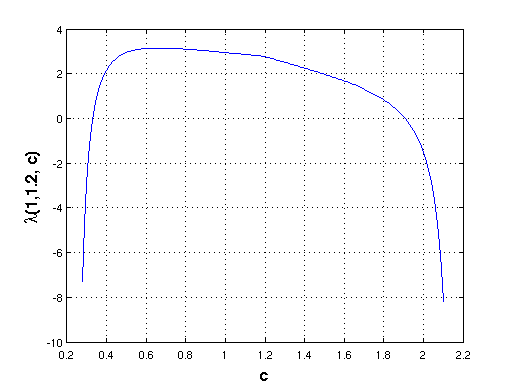
for any $t>0$. As an example, in Figure 1, we plot the graph of $\Lambda(a,b,c)$ with $a=1,b=1.2$ and $c$ varies from $(0.2,2.2)$.

Let $a,b,c$ be fixed real values with $0<a\leq b\leq c\leq a+b$. For any $k\in(\infty,\left(\frac{2\pi}{a+b+c}\right)^{2}]$, there exists a triangle $\Delta ABC$ in the model space $M_{k}^{2}$ with $a,b,c$ as its side lengths. We now consider the properties of $S(a,b,c,k)$ as a function of the variable $k\in(\infty,\left(\frac{2\pi}{a+b+c}\right)^{2}]$.

For any $k\in[\Lambda\left(a,b,c\right),\left(\frac{2\pi}{a+b+c}\right)^{2}]$, by the definition of $\Lambda(a,b,c)$, it follows that $\measuredangle ACB\geq\frac{2\pi}{3}$ in $M_{k}^{2}$. In this case, the minimum value of $S$ in (2.1) is achieved at the point $C$ and thus

For any $k\in(\infty,\Lambda\left(a,b,c\right))$, the angle $\measuredangle ACB<\frac{2\pi}{3}$ in $M_{k}^{2}$, and the minimum value of $S$ in (2.1) is achieved at the Fermat point $O$ in the interior of the triangle $\Delta ABC$. In this case,

where $x=\left|OA\right|_{k},y=\left|OB\right|_{k}$ and $z=\left|OC\right|_{k}$. Note that the angles $\measuredangle AOB=\measuredangle BOC=\measuredangle COA=\frac{2\pi}{3}$ in $M_{k}^{2}$.

We now calculate the value of $S(a,b,c,k)$ in (3.1) based on the signs of $k$.

Without losing of generality, we may assume that $d_{12}\leq d_{23}\leq d_{13}\leq d_{12}+d_{23}$.

Note that $g_{X}(T)\geq\frac{d_{12}+d_{23}+d_{13}}{2}$.

According to (2.2), we immediately have the following proposition:

For a real number $k$, a geodesic metric space $(X,d)$ is said to be CAT(k) if every geodesic triangle $\Delta ABC$ in $X$ with perimeter less than $2D_{k}$ satisfies the CAT(k) inequality. That is, let $\Delta A^{\prime}B^{\prime}C^{\prime}$ be a comparison triangle in the model space $(M_{k}^{2},\left|\cdot\right|_{k})$, with sides of the same length as the sides of $\Delta ABC$, such that for any $D$ in edge $BC$, there is a corresponding point $D^{\prime}$ in the comparison edge $B^{\prime}C^{\prime}$ with $d(B,D)=|B^{\prime}D^{\prime}|_{k},d(C,D)=|C^{\prime}D^{\prime}|_{k}$ and satisfies the inequality $d(A,D)\leq|A^{\prime}D^{\prime}|_{k}$.

References

- [1] M. R. Bridson and A. Haefliger, Metric Spaces of Non-positive Curvature, Springer-Verlag, Berlin Heidelberg, 1999.
- [2] D. Burago, Y. Burago, and S. Ivanov, A Course in Metric Geometry, in: Graduate Studies in Math., vol. 33, Amer. Math. Soc., Providence, RI, 2001.
- [3] Robin Forman, Bochner’s method for cell complexes and combinatorial Ricci curvature, Discrete Comput. Geom. 29:3 (2003), 323–-374.
- [4] John M. Lee, Riemannian Manifolds: An Introduction to Curvature. Graduate Texts in Mathematics, Vol. 176. (1997)
- [5] Emil Saucan, Curvature – Smooth, Piecewise-Linear and Metric, book chapter in What is Geometry?, Advanced Studies in Mathematics and Logic, 237-268, Polimetrica, Milano, 2006.
- [6] John M. Sullivan, Curvatures of Smooth and Discrete Surfaces. Discrete Differential Geometry, Oberwolfach Seminars 38, Birkhauser, 2008.