跳到论文正文
W Papers独立论文阅读器 arXiv:2109.01461 论文正文 计算阅读时间 · 0%
引用这篇论文根据当前论文元数据生成,正式投稿前建议核对。


License: CC BY-NC-SA 4.0
arXiv:2109.01461v2 [cs.LG] 04 Nov 2021

Dive into Layers: Neural Network Capacity Bounding using Algebraic Geometry

Ji YangEnflame-techEnflame-tech, 61 ShengXia Road, Pudong New District, Shanghaierik.yang@enflame-tech.com    Lu SangTechnical University of MunichBoltzmannstrasse 3, 85748 Garching, Germanysang@in.tum.deDaniel CremersTechnical University of MunichBoltzmannstrasse 3, 85748 Garching, Germanycremers@in.tum.de
Abstract

The empirical results suggest that the learnability of a neural network is directly related to its size. To mathematically prove this, we borrow a tool in topological algebra: Betti numbers to measure the topological geometric complexity of input data and the neural network. By characterizing the expressive capacity of a neural network with its topological complexity, we conduct a thorough analysis and show that the network’s expressive capacity is limited by the scale of its layers. Further, we derive the upper bounds of the Betti numbers on each layer within the network. As a result, the problem of architecture selection of a neural network is transformed to determining the scale of the network that can represent the input data complexity. With the presented results, the architecture selection of a fully connected network boils down to choosing a suitable size of the network such that it equips the Betti numbers that are not smaller than the Betti numbers of the input data. We perform the experiments on a real-world dataset MNIST and the results verify our analysis and conclusion. The demo code is publicly available†† https://github.com/Sangluisme/NeuralNetworkBettiNumber.

†† ∗ These authors contributed equally.

1 Introduction

Neural networks have rapidly become one of the most popular tools for solving challenging problems ([4, 25]) in various domains such as image understanding [18, 27], natural language processing [22, 30], and speech recognition [10]. In many cases, a major difficulty is to choose an appropriate size of the network that optimally balances the training cost and the expression structure in the data. Empirical results suggest that, for example, fully connected layers, i.e., dense layers with more hidden units, perform better than smaller layers with the same batches of inputs. However, too large networks can lead to excessive computational overhead or overfitting.

In computer vision, some works such as [2, 13, 38] use Neural Architecture Search (NAS) to determine the architecture of a network, since they treat architecture selection as a compositional hyperparameter. The advantage of their methods is that they can deal with different types of layers, such as convolution or pooling layer. Some other works  [34, 35] try to improve initial architecture selection. However, their results are difficult to interpret beyond empirical optimality. Despite the success of these approaches, there is still no general principle for architecture selection.

In this paper, we exploit a topological invariant, i.e., Betti numbers, to describe the expressiveness of a neural network architecture given the input data, which is formally introduced in Section 2. Once Betti numbers are used to describe the topological geometric complexity of a structure, a network with efficient expressiveness must represent the topological complexity of the input data, in other words, the Betti numbers at each layer can not be smaller than the Betti numbers of the input data. As we will introduce in Section 3, the upper bounds on the Betti numbers of each layer are determined by the number of hidden units and layer numbers. Thus, a relation is established between the scales of a network and the topological complexity of the input data. Since the Betti numbers of the input data can be precomputed, our results give a clear indication of the relationship between the size of dense layers and their expression capabilities.

1.1 Our Contribution

In this paper, we focus on fully connected networks or multilayer perceptrons (MLPs) with polynomial or ReLU activation, which are widely used ([6, 26, 28]). The impact of the layer size on the performance is analyzed. A fully connected layer can be interpreted as an operator that maps the input into a quotient space (equivalent classes). Given a neural network for classification tasks, a successfully trained network means that the input is mapped to the correct classes. We traverse back to each layer to examine the pre-images of the output classes, and these pre-images are sequences of sets endowed with certain topological properties, these specific topological structures allow us to bound their Betti numbers. a) We use Betti numbers as a quantitative measure of the topological complexity of a network consists of dense layers with ReLU or polynomial activations. b) We derive the upper bounds on the Betti numbers of each layer and show that the architecture selection problem can be characterized by endowing the "efficient topological capacity" of each layer. c) Our results provide mathematical insight into the performance of a network and its capacity. d) In addition, we verify our theoretical results using the MNIST[24] dataset to show that understanding topological complexity is beneficial in determining the structure of the neural network.

2 Background

2.1 Topology and Algebraic Topology

Topology, used in this paper refers mainly to topological geometry. Topology is a mathematical branch that studies the properties of objects that are preserved by deformation, twisting, rotation, and extension. From a topological point of view, two objects (or spaces) XX and YY are said to be equivalent if there is a continuous function f:X→Yf:X\to Y which has a continuous inverse f−1f^{-1}. XX and YY are called homeomorphic and ff is their homeomorphism. The advantage of using topological properties to characterize data or network structures is that these properties are invariant to some irrelevant features such as scaling, rotation, translation, etc. Using topological complexity to describe the capacity of a network provides an "outline structure" of the output domain.

Algebraic topology studies the intrinsic qualitative aspects of spatial objects. It uses algebraic concepts such as groups and rings to represent topological structures. Algebraic topology provides a great tool to analyze and compute the structures of spaces. Simply speaking, algebraic topology studies the’ hole’ structures of a space. The complexity of the topological geometry is then characterized by the number of ’holes’ in different dimensions that space contains. Therefore, a space is divided into simplex cells into different dimensions. Simplex cells are generalized triangles that can be considered as the basis of a topological space. A space is formed by gluing cells together in a particular way. These "glued together" cells form simplical complex. Intuitively, a simplex can be thought as a discretization of a space into triangles that are glued together. After using algebraic topology to assign groups to these cells, the homology tool can be used.

2.2 Homology and Persistent Homology

Homology-

Homology groups are mainly used in this paper. Informally, the nn-th homology group of a topological space XX, denoted Hn​(X)H_{n}(X) describes the number of nn-th dimensional "holes" in XX, the 0−0-dimensional hole being the connected component of the space. More strictly, for a topological space XX, one first constructs a chain complex C⁡(X)C(X) that encodes information about XX. Usually, this is a sequence of abelian groups C0,C1,…C_{0},C_{1},\dots, connected by the function δi:Ci→Ci−1\delta_{i}:C_{i}\to C_{i-1} which preserves the group structure, the functions are group homomorphisms called boundary operators. The chain complex can be constructed by continuous mappings from the simplex cell to XX. Then the homology group is defined as Hn​(X)=Ker⁡δn/Im⁡δn+1H_{n}(X)=\Ker\delta_{n}/\Img\delta_{n+1}, i.e., the quotient group of kernel of δn\delta_{n} and image of δn+1\delta_{n+1}. C⁡(X)C(X) reflects the structure of XX.

Betti Number-

The nn-th Betti number bnb_{n} of the set XX is the rank of the homology group Hn​(X)H_{n}(X), which specifies the maximum number of cuts that can be made before a surface is decomposed into an nn-th dimensional simplex. Geometrically, the ii-th Betti number refers to the ii-th dimensional holes in space XX. For example, for a circle 𝕊1{\mathbb{S}}^{1}, the ii-th homology group Hi​(𝕊1)H_{i}({\mathbb{S}}^{1}) is zero if ii is greater than 11, since there is no higher dimensional hole; Hi​(𝕊1)=ℤH_{i}({\mathbb{S}}^{1})={\mathbb{Z}} for i=0,1i=0,1 and b0​(𝕊1)=b1​(𝕊1)=1b_{0}({\mathbb{S}}^{1})=b_{1}({\mathbb{S}}^{1})=1 because 𝕊1{\mathbb{S}}^{1} has a connected component and a 1-dimensional hole; for more details see [20]. Similarly, an nn-dimensional sphere Hi​(𝕊n)H_{i}({\mathbb{S}}^{n}) is nontrivial if and only if ii is 00 or nn, i.e. Hi​(𝕊n)=ℤH_{i}({\mathbb{S}}^{n})={\mathbb{Z}} for i=0i=0 and nn, since the nn-dimensional sphere 𝕊n\mathbb{S}^{n} has a connected component and an nn-dimensional hole.

Persistent Homology and TDA-

To compute Betti numbers for arbitrary topological spaces, we borrow the tool of persistent homology. Persistent homology computes topological properties of a space that are invariant to a particular choice of parameters, e.g., a torus has two 1-D holes (b0=1,b1=2,b2=0,⋯b_{0}=1,b_{1}=2,b_{2}=0,\cdots), regardless of the inner or outer radius, its orientation or position. The main procedure for finding the persistent homology in a space with simplicial complex structure is to find a real-valued function ff satisfying some certain properties on these complices KK, so that we can form a filtration of the level set KiK_{i} (K(a)=f−1(−∞,a]K(a)=f^{-1}(-\infty,a]), i.e., ∅=K0⊂K1⊂⋯⊂Kn=K\emptyset=K_{0}\subset K_{1}\subset\dots\subset K_{n}=K. Using the properties of filtration, for each dimension nn we can find the homomorphism on the simplicial homology groups Hp​(Ki)H_{p}(K_{i}) to Hp​(Kj)H_{p}(K_{j}), the pp-th persistent homology groups are the images of these homomorphisms, and the nn-th persistent Betti numbers bni,jb_{n}^{i,j} are rank of these groups. With the persistent homology properties, we are allowed to represent the persistent homology with barcode or persistent diagram.

Persistent homology is the crucial tool for Topological Data Analysis (TDA), which extracts the high dimensional information from datasets. It provides a general framework to analyze the data regardless of the chosen metric and to compose discrete points into a global structure. TDA is used to analyze and visualize the persistent homology. In the computational process, given a collection of points {xi}\{x_{i}\} in ℝd\mathbb{R}^{d}, first, one type of the complex is computed under certain criteria. Then the persistent homology on the complex is determined. As Figure 1 shows, a persistent barcodes graph is used to visualize the homological structures on the dataset.

Refer to caption Refer to caption
Figure 1: An example of the barcode for H∗​(X)H_{*}(X) where XX is a set of growing balls. Clearly the sets {Xϵ}\{X_{\epsilon}\} form a filtration where ϵ\epsilon is the radius of each ball. The rank of Hk​(Xϵi)H_{k}(X_{\epsilon_{i}}) equals the numbers of intervals in the barcode for H∗​(X)H_{*}(X) intersecting a vertical line ϵ=ϵi\epsilon=\epsilon_{i} [11]. The red bars are zero-order Betti numbers and the blue bars represent the first-order Betti numbers. Different bars are Betti numbers correspond to different generator. Draw a vertical line at ϵ0\epsilon_{0} from x-axis and intersect with the bars can find the rank of H0​(Xϵ0)H_{0}(X_{\epsilon_{0}}) or H1​(Xϵ0)H_{1}(X_{\epsilon_{0}}) for a certain generator.

A barcodes graph is a graphical representation of Hk​(X)H_{k}(X) as a collection of horizontal line segments in a plane. The horizontal axis corresponds to the radius of the generated complex and the vertical axis is an ordering of the homology generators.

2.3 Preliminary Results

The characterization of homology structure on a neural network and the relationship between Betti numbers and the learning ability of a neural network have been used in some previous work. The work of Bianchini and Scarsellii [5] gives the upper bounds on the sum of Betti numbers on a binary classification network with a shallow or strictly constrained deep neural network based on Pfaffian sets, with polynomial activation cases only. The bounds are up to O⁡(deg⁡(P)n​l)O(\deg(P)^{nl}), where nn is the number of nodes and ll is the number of layers, and deg⁡(P)\deg(P) is the degree of the polynomial. The work of Guss et al [19]. gives an empirical analysis on the effect of the number of hidden units of the first layer on the performance of a classification network using algebraic topology. Other work has focused on finding the Betti number range on various mathematical structures such as semi-algebraic sets ([3, 14]). Our work extends the mathematical results and applies them to nn-classifying neural networks. We are able to bound the Betti numbers of each layer, the bound is tight up to O⁡((l​deg⁡(P))n)O((l\deg(P))^{n}), and our results are applicable to ReLU. This is archived by extracting the algebraic structure on the layer to form semi-algebraic sets, which is a different approach than using Paffian functions.

3 Homological Structure of Neural Networks

In this section, we will analyze the homology structure on each layer of a neural network. First, let us define the topological structure on neural architectures. A feedforward nn-classification neural network 𝒩:ℝd→{1,2,⋯,n}\mathcal{N}:\mathbb{R}^{d}\rightarrow\{1,2,\cdots,n\} is given by the composition

𝒩=s∘fl∘σ∘fl−1⋯σ∘f1(x).\mathcal{N}=s\circ f_{l}\circ\sigma\circ f_{l-1}\cdots\sigma\circ f_{1}(x)\>. (1)

Each layer acts as an affine transformation fj:ℝnj→ℝnj+1,j=1,2,⋯,l−1f_{j}:\mathbb{R}^{n_{j}}\to\mathbb{R}^{n_{j+1}},j=1,2,\cdots,l-1 and σ:ℝnj+1→ℝnj+1\sigma:\mathbb{R}^{n_{j+1}}\to\mathbb{R}^{n_{j+1}} is the activation of this layer. The softmax or sigmoid function on the last layer is denoted as s:ℝn→ℝns:\mathbb{R}^{n}\to\mathbb{R}^{n}. Then the network has ll layers, the number of hidden units on layer jj is njn_{j}, and the ll-th layer is the output layer that maps the input data to nn classes. Now consider the output set of the neural network S=⋃j=1nS⁡(j)S=\bigcup_{j=1}^{n}S(j), where S⁡(j)⊂SS(j)\subset S is the set of the jj-th class, i.e., S⁡(j)S(j) is the image of s∘fls\circ f_{l} in class jj. Traversing these classified sets back to the ii-th layer, we obtain the pre-images of S⁡(j)S(j) on the ii-th layer, denoted Si​(j)S^{i}(j). Then the topological invariant of each layer is characterized by the property of the sets {Si​(j)}ji\{S^{i}(j)\}_{j}^{i}. However, due to the unknown sign of the elements in the weight matrices, one encounters a system of inequalities when directly analyzing the topological properties of {Si​(j)}ji\{S^{i}(j)\}_{j}^{i}. To avoid the problem, we have instead focused on the boundary sets ∂Si​(j)\partial S^{i}(j) of the pre-images instead, which are the solution of a system of equations, and the properties of {Si​(j)}ji\{S^{i}(j)\}_{j}^{i} can be characterized by these boundary sets using the Mayer-Vietoris sequence, more details will be presented in the coming sections.

The boundary of the set Si​(j)S^{i}(j) is the ambiguous set associated to the jj-th class, i.e. the mapping from the ii-th layer to the output is Fi=s∘fl∘σ∘fl−1​…​σ∘fi​(x):ℝni→ℝnF_{i}=s\circ f_{l}\circ\sigma\circ f_{l-1}\dots\sigma\circ f_{i}(x):\mathbb{R}^{n_{i}}\to\mathbb{R}^{n} for the nn classifier and Fi=[Fi1,…,Fin]F_{i}=[F^{1}_{i},...,F_{i}^{n}] has nn components. If x0x_{0} is mapped to class jj, then the jj-th component Fij​(x0)F_{i}^{j}(x_{0}) is said to have value greater than the other component Fik​(x0),k≠jF_{i}^{k}(x_{0}),~k\neq j. The boundary of the jj-th class ∂Si​(j)\partial S^{i}(j) is {x∈ℝni|∃k s.t Fik(x)=Fij(x),Fij(x)≥Fip(x),p≠j,k}\{x\in\mathbb{R}^{n_{i}}|\exists k\text{ s.t }F_{i}^{k}(x)=F_{i}^{j}(x),F_{i}^{j}(x)\geq F_{i}^{p}(x),p\neq j,k\}. Thus, the set can be decomposed according to the number of equal component functions by a set of equalities and inequalities forming a submanifold. The classical Mayer-Vietoris sequence gives the relation over the homology groups between their intersection and union of two topological manifolds.

3.1 Algebraic Structure of Dense Layers

We go further and examine the properties of this boundary set. Every Si​(j)S^{i}(j) has a decomposition or a covering of semi-algebraic sets. A semi-algebraic set (in the field of real numbers) is a subset SS of ℝn\mathbb{R}^{n} defined by a finite sequence of polynomial equations and inequalities, or any finite union of such sets. For simplicity, for the ii-th dense layer, fi​(x)=Wi​Xi+Bif_{i}(x)=W^{i}X^{i}+B^{i}, where WiW^{i} is the weight matrix and BiB^{i} is the bias vector. If the layer is equipped with polynomial activation, (σ∘fi)​(x)=P⁡(Wi​Xi+Bi)(\sigma\circ f_{i})(x)=P(W_{i}X^{i}+B_{i}), where P=[Q1i,…,Qnii]P=[Q^{i}_{1},\dots,Q^{i}_{n_{i}}] is the polynomial activation on the ii-th layer. Thus, the pre-images of the layers are the composition of the algebraic sets. For simplicity, we give the results as two lemmas only; the proof details can be found in the appendix.

Lemma 1.

For a nn-classification network (n≥2n\geq 2) has structure defined in (1) and σ\sigma is the polynomial activation (degree less than rr), the boundary set ∂Si​(j)\partial S^{i}(j) has the following covers

∂Si(j)=⋃p≠j({Qji−Qpi=0}∩{Qji−Qqi≥0,q≠p,j})=⋃p≠jSpi(j),\partial S^{i}(j)=\bigcup_{p\neq j}(\{Q^{i}_{j}-Q^{i}_{p}=0\}\cap\{Q^{i}_{j}-Q^{i}_{q}\geq 0,q\neq p,j\})=\bigcup_{p\neq j}S^{i}_{p}(j)\>, (2)

where Qji,1≤j≤nQ^{i}_{j},1\leq j\leq n is the jj component polynomial function on the ii-th layer with deg⁡(Qji)≤r⁡(l−i−1)\deg(Q^{i}_{j})\leq r(l-i-1). Moreover, for a sub index set {α0,…,αp}\{\alpha_{0},\dots,\alpha_{p}\} of {1,2,…,j−1,j+1,…,n}\{1,2,\dots,j-1,j+1,\dots,n\}, then Sα0​…​αpi(j)=Sα0i(j)∩⋯∩Sαpi(j)={Qji−Qαki=0,k=0,…,p}∩{Qji−Qqi≥0,q≠α0,…,αp,j}S^{i}_{\alpha_{0}\dots\alpha_{p}}(j)=S^{i}_{\alpha_{0}}(j)\cap\dots\cap S^{i}_{\alpha_{p}}(j)=\{Q^{i}_{j}-Q^{i}_{\alpha_{k}}=0,k=0,\dots,p\}\cap\{Q^{i}_{j}-Q^{i}_{q}\geq 0,q\neq\alpha_{0},\dots,\alpha_{p},j\}.

Lemma 2.

For a nn-classification network (n≥2n\geq 2) has structure defined in (1) with ReLU activation whose weight matrices are always full ranks, the pre-images on the boundary of the jj-th class on the ii-th layer ∂Si​(j)\partial S^{i}(j) has the cover

∂Si(j)=⋃p≠jSpi(j),andSα0⋯αpi(j)=Sα0i(j)∩⋯∩Sαpi(j)\partial S^{i}(j)=\bigcup_{p\neq j}S^{i}_{p}(j),~~\text{and}~~S^{i}_{\alpha_{0}\cdots\alpha_{p}}(j)=S^{i}_{\alpha_{0}}(j)\cap\cdots\cap S^{i}_{\alpha_{p}}(j) (3)

for sub index set {αk}k\{\alpha_{k}\}_{k} defined the same as in lemma 1. The cover is determined by the following equations

Xl−11=−W~1−1B~α0⋯αp−W~1−1W~2Xl−12,\displaystyle X^{l-1}_{1}=-\widetilde{W}_{1}^{-1}\widetilde{B}_{\alpha_{0}\cdots\alpha_{p}}-\widetilde{W}_{1}^{-1}\widetilde{W}_{2}X^{l-1}_{2}\>,
X1l−2=−(W1l−2)−1​(B~l−1−Bl−1)−(W1l−2)−1​W2l−2​X2l−2,\displaystyle X^{l-2}_{1}=-(W^{l-2}_{1})^{-1}(\widetilde{B}^{l-1}-B^{l-1})-(W^{l-2}_{1})^{-1}W^{l-2}_{2}X^{l-2}_{2}\>,
⋯\displaystyle\cdots
X1i=−(W1i)−1​(B~i+1−Bi+1)−(W1i)−1​W2i​X2i,\displaystyle X^{i}_{1}=-(W^{i}_{1})^{-1}(\widetilde{B}^{i+1}-B^{i+1})-(W^{i}_{1})^{-1}W^{i}_{2}X^{i}_{2}\>,

where Wi=(wi​ji)∈ℝni×ni−1W^{i}=(w^{i}_{ij})\in\mathbb{R}^{n_{i}\times n_{i-1}} is the weight matrix Bi=[b0i,…,bnii]B^{i}=[b^{i}_{0},\dots,b^{i}_{n_{i}}] is the bias vector on the ii-th layer.

B~α0​…​αp=[bjl−bα0l,bjl−bα1l,…​bjl−bαpl]⊤,\displaystyle\widetilde{B}_{\alpha_{0}\dots\alpha_{p}}=\left[b^{l}_{j}-b^{l}_{\alpha_{0}},b^{l}_{j}-b^{l}_{\alpha_{1}},\dots b^{l}_{j}-b^{l}_{\alpha_{p}}\right]^{\top}\>,
[W~1W~2]=W~α0⋯αp=[wj,1l−1−wα0,1l−1wj,2l−1−wα0,2l−1⋯wj,nl−1l−1−wα0,nl−1l−1wj,1l−1−wα1,1l−1wj,2l−1−wα1,2l−1⋯wj,nl−1l−1−wα1,nl−1l−1⋱wj,1l−1−wαp,1l−1wj,2l−1−wαp,2l−1⋯wj,nl−1l−1−wαp,nl−1l−1],\displaystyle\begin{bmatrix}\widetilde{W}_{1}&\widetilde{W}_{2}\end{bmatrix}=\widetilde{W}_{\alpha_{0}\cdots\alpha_{p}}=\begin{bmatrix}w^{l-1}_{j,1}-w^{l-1}_{\alpha_{0},1}&w^{l-1}_{j,2}-w^{l-1}_{\alpha_{0},2}&\cdots&w^{l-1}_{j,n_{l-1}}-w^{l-1}_{\alpha_{0},n_{l-1}}\\ w^{l-1}_{j,1}-w^{l-1}_{\alpha_{1},1}&w^{l-1}_{j,2}-w^{l-1}_{\alpha_{1},2}&\cdots&w^{l-1}_{j,n_{l-1}}-w^{l-1}_{\alpha_{1},n_{l-1}}\\ \vdots&\vdots&\ddots&\vdots\\ w^{l-1}_{j,1}-w^{l-1}_{\alpha_{p},1}&w^{l-1}_{j,2}-w^{l-1}_{\alpha_{p},2}&\cdots&w^{l-1}_{j,n_{l-1}}-w^{l-1}_{\alpha_{p},n_{l-1}}\end{bmatrix}\>,
B~i+1=[−(W1i+1)−1​(B~i+2−Bi+2)0]+[−(W1i+1)−1​W2i+1I]​X2i+1=[X1i+1X2i+1],\displaystyle\widetilde{B}^{i+1}=\begin{bmatrix}-(W^{i+1}_{1})^{-1}(\widetilde{B}^{i+2}-B^{i+2})\\ 0\end{bmatrix}+\begin{bmatrix}-(W^{i+1}_{1})^{-1}W^{i+1}_{2}\\ I\end{bmatrix}X^{i+1}_{2}=\begin{bmatrix}X^{i+1}_{1}\\ X^{i+1}_{2}\end{bmatrix}\>,

and Wk=[W1k,W2k]W^{k}=\left[{W}^{k}_{1},{W}^{k}_{2}\right], W1kW^{k}_{1} is the reversible sub-matrix of full rank matrix WkW^{k} and the inequalities.

Xl−1∈ℝ+nl−1,Xl−2∈ℝ+nl−2,⋯,Xi∈ℝ+niX^{l-1}\in\mathbb{R}_{+}^{n_{l-1}},X^{l-2}\in\mathbb{R}_{+}^{n_{l-2}},\cdots,X^{i}\in\mathbb{R}_{+}^{n_{i}}
[Xjl−Xql]\displaystyle\begin{bmatrix}X^{l}_{j}-X^{l}_{q}\end{bmatrix} =[wj,1l−1−wq,1l−1wj,2l−1−wq,2l−1⋯wj,nl−1l−1−wq,nl−1l−1]​[X1l−1X2l−1…Xnl−1l−1]⊤\displaystyle=\begin{bmatrix}w^{l-1}_{j,1}-w^{l-1}_{q,1}&w^{l-1}_{j,2}-w^{l-1}_{q,2}&\cdots&w^{l-1}_{j,n_{l-1}}-w^{l-1}_{q,n_{l-1}}\\ \end{bmatrix}\begin{bmatrix}X^{l-1}_{1}&X^{l-1}_{2}&\dots&X^{l-1}_{n_{l-1}}\end{bmatrix}^{\top}
+[bjl−bql]≥0\displaystyle+\begin{bmatrix}b^{l}_{j}-b^{l}_{q}\end{bmatrix}\geq 0

where q≠α0,⋯,αp,jq\neq\alpha_{0},\cdots,\alpha_{p},j.

Using subindex set {αk}k\{\alpha_{k}\}_{k} to build the new cover of Si​(j)S^{i}(j) is for using generalized Mayer-Vietoris sequence later, such that we can use the Betti numbers of covering sets to bound the Betti numbers of the whole set.

3.2 Betti numbers on the Neural Architectures

Each layer of the neural network was characterized by a semi-algebraic set covering. The work of Basu et al. [3] derived the upper bound on the Betti numbers for a semi-algebraic set; other work ([29, 21, 37]) derived the upper bounds on the maximum sum of Betti numbers of any algebraic set defined by polynomials. To bound the Betti numbers on each layer, we need to prove the inequalities of the Betti numbers for individual sets and their union. The main steps to establish the relation are: first, ∂Si​(j)=Si​(j)¯∩U/Si​(j)¯\partial S^{i}(j)=\overline{S^{i}(j)}\cap\overline{U/S^{i}(j)}, in the polynomial case U=ℝniU=\mathbb{R}^{n_{i}} and in the ReLU case U=ℝ+niU=\mathbb{R}_{+}^{n_{i}}. The boundary set can then be described by the closure of pre-images of each class on each layer. Next, we generalize the Mayer-Vietoris sequence to be suitable for nn covering a set ∂Si​(j)\partial S^{i}(j). Second, we use the Mayer-Vietoris sequence to show that the Betti numbers of the set ∂Si​(j)\partial S^{i}(j) are not larger than the sum of the Betti numbers of the individual cover sets Sαo,…,αpi​(j)S^{i}_{\alpha_{o},\dots,\alpha_{p}}(j) in (2) and (3). That is, if S1,S2,…,SnS_{1},S_{2},...,S_{n} is the cover of the set SS, then the kk-th Betti number of the set bk​(S)b_{k}(S) satisfies.

bk(S)≤∑i+j=k∑J⊂{1,2,..,n}|J|=j+1bi(SJ).b_{k}(S)\leq\sum_{i+j=k}\sum_{J\subset\{1,2,..,n\}\left|J\right|=j+1}b_{i}(S_{J})\>. (4)

Here JJ is a subindex set like {αi}i\{\alpha_{i}\}_{i} in Lemma 1 and 2, |J|\left|J\right| is the number of sets. This inequality is derived by proving that the rank of the homological group of the set SS is less than the sum of the ranks of the intersections of its covers. Finally, we apply the results of Basu et al [3]. and Milnor et al [29]. to find upper bounds on Betti numbers. The details of the proofs can be found in the appendix. The main result is derived after all the procedures have been collected.

Theorem 1.

Suppose a neural network 𝒩\mathcal{N} has structure as defined in (1) with polynomial activation PP (deg⁡(P)≤r\deg(P)\leq r), L={Li|l≥i≥0,dim(Li)=ni}L=\{L_{i}|l\geq i\geq 0,\dim(L_{i})=n_{i}\} denotes the layers of the neural network and nl=nn_{l}=n, and assume this neural network has a non-increasing structure, i.e., np≤nq,p≥qn_{p}\leq n_{q},p\geq q, then the Betti numbers of the closure of the jj-th class pre-image on the ii-th layer Si​(j)¯\overline{S^{i}(j)} are bounded by the following inequalities:

bk(Si​(j)¯)≤{∑p=0k(n−1p+1)⁡(3n−2−p−1)​r​(l−i−1)​(2​r​(l−i−1)−1)ni−1,k<n−2,(∑p=0n−3(n−1p+1)⁡(3n−2−p−1)+1)​r​(l−i−1)​(2​r​(l−i−1)−1)ni−1,k≥n−2,b_{k}(\overline{S^{i}(j)})\\ \leq\left\{\begin{aligned} &\sum_{p=0}^{k}\binom{n-1}{p+1}(3^{n-2-p}-1)r(l-i-1)(2r(l-i-1)-1)^{n_{i}-1},&k<n-2,\\ &\left(\sum_{p=0}^{n-3}\binom{n-1}{p+1}(3^{n-2-p}-1)+1\right)r(l-i-1)(2r(l-i-1)-1)^{n_{i}-1},&k\geq n-2,\end{aligned}\right.

for i<l−1i<l-1. On the (l−1)(l-1)-th layer

bk(Sl−1​(j)¯)≤{∑p=0k(n−1p+1)⁡(3n−2−p−1),k<n−2,∑p=0n−3(n−1p+1)⁡(3n−2−p−1)+1,k≥n−2.b_{k}(\overline{S^{l-1}(j)})\\ \leq\left\{\begin{aligned} &\sum_{p=0}^{k}\binom{n-1}{p+1}(3^{n-2-p}-1),&k<n-2,\\ &\sum_{p=0}^{n-3}\binom{n-1}{p+1}(3^{n-2-p}-1)+1,&k\geq n-2\>.\end{aligned}\right.
Theorem 2.

Suppose a neural network 𝒩\mathcal{N} has structure as defined in (1) with ReLU activation, L={Li|l≥i≥0,dim(Li)=ni}L=\{L_{i}|l\geq i\geq 0,\dim(L_{i})=n_{i}\} denotes the layers of the neural network and nl=nn_{l}=n, and assume this neural network has a non-increasing structure, i.e., np≤nq,p≥qn_{p}\leq n_{q},p\geq q, then the Betti numbers of the closure of the jj-th class pre-image on the ii-th layer Si​(j)¯\overline{S^{i}(j)} are bounded by the following inequalities:

bk(Si​(j)¯)≤{∑p=0k(n−1p+1)⁡(3∑q=l−1inq+n−2−p−1),k<n−2,∑p=0n−2(n−1p+1)⁡(3∑q=l−1inq+n−2−p−1),k≥n−2.b_{k}(\overline{S^{i}(j)})\\ \leq\left\{\begin{aligned} &\sum_{p=0}^{k}\binom{n-1}{p+1}(3^{\sum_{q=l-1}^{i}n_{q}+n-2-p}-1),&k<n-2\>,\\ &\sum_{p=0}^{n-2}\binom{n-1}{p+1}(3^{\sum_{q=l-1}^{i}n_{q}+n-2-p}-1),&k\geq n-2\>.\end{aligned}\right.

4 Homological Neural Network Architecture Selection

In the previous section 3 we derived the upper bounds of the Betti numbers at each layer. However, the practical use of Betti numbers must apply to the real data. To validate our conclusion and demonstrate the interpretation of the derived results, a dataset MNIST ([24]) are used for testing. The persistent homology is computed using the Python library GUDHI [36]. We focus on the zero-order and first-order topological features, i.e., b0b_{0} and b1b_{1} for each class, to characterize the neural network complexity, because the package copes better with lower-dimensional homological features than with higher dimensions.

4.1 Expression Ability

We validate our conjecture that the Betti numbers of the layers reflect the expressiveness of the network. We build networks with the architecture shown in Figure 2 with different hidden units; each dense layer has the same hidden units in each network. The layer number l=4l=4 and we tested the hidden units nin_{i} for i=1,2,3i=1,2,3 from 2 to 147. We take the output of the ten different classes from the third layer (the layer before Softmax) and computed their zero-order and first-order Betti numbers b0ib_{0}^{i}, b1ib_{1}^{i} for i=1,…,10i=1,\dots,10. Note that batch normalization is added because the persistent homology barcodes are computed with respect to a certain radius.

Refer to caption Refer to caption
(b) input data Betti numbers (c) inefficient presentation
Refer to caption Refer to caption
(a) (d) efficient representation (e) output b0b_{0} and accuracy
Figure 2: ((a) Network structure: the network has 3 fully connected layers with ReLU activation and batch normalization. (b)-(d) A network with sufficient expression ability should have sufficient topology complexity to represent the geometry of the input data. (e) The varying number of hidden units affects the complexity of the network. If a network can achieve a certain accuracy, the layer output (the pre-images of the classes) should have b0b_{0} converging with the b0b_{0} of the input data.

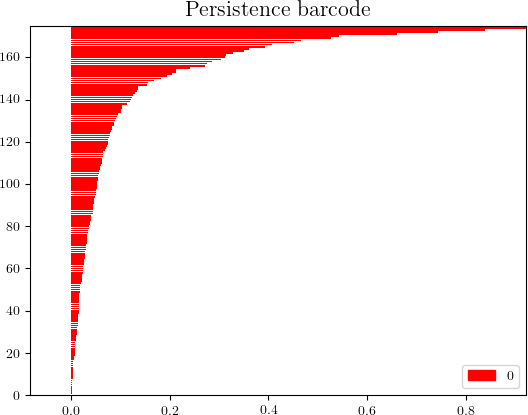
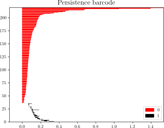
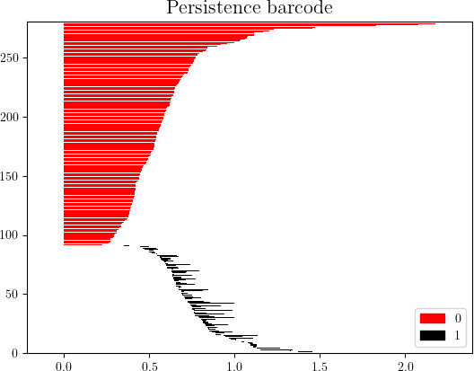
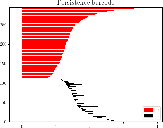
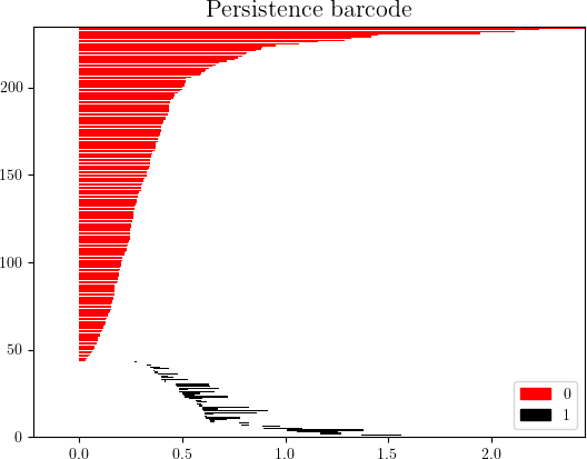
The b0b_{0} of class 4 and the persistent homology barcodes are shown in Figure 2. In the inefficient representation, the persistent barcode graph behaves dissimilarly and cannot interpret the first-order features, also shown in Figure 5. The efficient representation occurs when the layers equip enough hidden units and can express more topological structure than the input data. Our presented theorems prove that expressiveness is determined by the number of layers and the number of hidden units of a dense neural network. Note that the dense layers are affine transformations and should not increase the topological structures of the input data. Thus, when the node number increases, the Betti numbers of the layer output will not unlimitedly increase, they should be close to the Betti numbers of the input data. We take the maximum b0b_{0} with a minimum radius of the 10 classes pre-images from the third layer and compare them with the input data b0b_{0}, plotted in Figure 2 (c). If the network achieves a certain accuracy, the Betti numbers are close to the input data.

Refer to caption Refer to caption
output b0b_{0} class 6 output b0b_{0} class 9
Figure 3: Investigate the output b0b_{0} of class 6 and class 9 on the third layer of the neural network with different layer size. The b0b_{0} increases with layer size and tries to be consistent with the input data b0b_{0}.
Refer to caption Refer to caption Refer to caption Refer to caption
node = 7 node = 37 node = 142 input class 6
Refer to caption Refer to caption Refer to caption Refer to caption
node = 7 node = 27 node = 142 input class 9
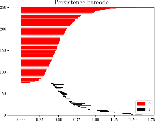
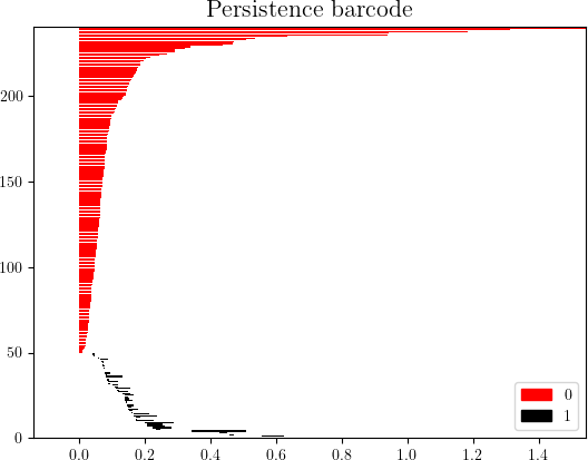
Figure 4: The graphs in the first row are persistent barcodes of class 6 and the second row is of class 9. The graphs in the first three columns correspond to the node numbers pointed to by the three red arrows in each graph in Figure 4. The graphs in the last column are the barcodes of the input classes. The inefficient representation occurs when b0b_{0} is significantly smaller than the input data b0b_{0} and the persistent barcode graph is different from the barcode graph of the input data barcodes graph. When the layer interprets the input data efficiently, the output and input barcode graphs have the similar structure.

The Figure 4 shows the b0b_{0} in different layer size with ReLU activation of class 6 and class 9. As accuracy increases, the b0b_{0} tents converge to the input data b0b_{0}. And the Figure 4 shows the persistent homology barcodes of certain layer sizes.

Refer to caption Refer to caption Refer to caption Refer to caption
output b0b_{0} node = 5 node = 7 node = 17
Figure 5: When a neural network are not well trained, the layer fails to represent the homology structure of the input data. Take class 9 as an example, the input data barcodes graph is shown in Figure 4. The blue line is the test error of the inefficient representation and the red line is the test error of a well trained network. Plot the barcodes graphs at the three red arrows, they all show different structures from inpout data.

4.2 Betti Numbers Bounding Interpretation

Theorem 1 and Theorem 2 show that the upper bounds of Betti numbers for each layer decrease as the layer index increases, i.e., if all layers are of equal size, then the upper bounds of Betti numbers are descending along with the layers. Note that if there is no other operation between two dense layers that can increase the topological structure of the input, e.g., only fully connected layers in the network, since the dense layer only applies an affine transformation to the data, it will not increase the topological feature. This means that a neural network should be equipped with enough hidden units of the first dense layer to have sufficient topological complexity to represent the input data. As a decreasing networks, even though without any activation, the affine transforamtion is a projection from high dimensional space to a low dimensional space, the betti numbers will naturally decreasing. The same conclusion was drawn by Guss et al. in [19], who proposed that the choice of the size of the first layer determines the learning ability of the network. Our theoretical work is consistent with their experimental results.

Refer to caption Refer to caption
(a) (b)
Figure 6: (a) For a network with three equal-size dense layers (with polynomial activation), change the layer size, Betti numbers of the different layers are descending along the layers. (b) The homology structures within the layers are preserved if the number of hidden nodes is sufficient and the complexity of the input exceeds the expressiveness of a network with fewer nodes. Here are the layers with ReLu activation.

We validate our interpretation against the MNIST dataset, as Figure 6 shows. The average b0b_{0} with minimum radius from the 10 classes on each layer are taken. In the left graph, relatively small nodes are taken so that the expression capacities of the layers (with polynomial activation) may not exceed the input data. The output Betti numbers on each layer tend to decrease along with the layers. In the case of ReLU activation, we see how Betti numbers are kept among layers. As larger layer sizes are chosen, the complexity of the network exceeds the complexity of the input data, hence the b0b_{0} are quite similar among layers since they are bounded by the input data b0b_{0}.

The second observation from the derived theorems is that the upper bounds increase with the size of the layer. In other words, layers with more hidden units are more likely to have the efficient expressive ability. This observation has been known for a long time. Our results provide a mathematical explanation for the conjecture. In Figure 7, different hidden units were chosen for a layer and the b0b_{0} on that layer was calculated. Note that relatively fewer node numbers were chosen to ensure that the homology complexity of the layer does not exceed the complexity of the input data. Otherwise, as explained earlier, the layer, although having more complexity, would only maximally represent the complexity of the input data.

Refer to caption Refer to caption
(a) (b)
Figure 7: Given a three dense layers network, examine the b0b_{0} on one of the three layers by changing the layer size. The Betti numbers of the different layer sizes are in ascending order. The left graph is the layer with polynomial activation and the right graph is the layer with ReLU activation.

5 Conclusion and Future Work

This work follows from the seminal work ([9, 12, 5]) that attempted to understand the expressiveness of neural network architectures and to exploit the expressive capacity of each layer of a neural network in the language of topological complexity. Our algebraic view characterizes the expressivity through topological invariants: Betti numbers and we derive the upper bounds on the Betti numbers on each layer of a neural network. The empirical question of the performance and learnability of a network can then be explained mathematically. Compared to previous work, our results provide explicit upper bounds on the topological complexity at each layer of a network and provide theoretical evidence for observed conjectures in the choice of a neural network’s architecture that goes beyond empirical conclusions. The presented work extracts the data and neural networks topological features and assigns a computable measure to describe the architecture power. Then the architecture selection problem is boiled down to chose a suitable network size according to the measure. Moreover, our results and conjectures are verified in a real-world dataset.

There are several possible avenues for the following future research. First, it is possible to extend the holomogical complexity analysis to other types of layers such as convolutional layers, since convolutional layers share some linearities with dense layers [26]. Second, the bounds on Betti numbers could be further tightened. However, further tightening of the bounds depends on a better related spectral theory that can bound the Betti numbers on semi-algebraic sets, and a smaller covering of the pre-images can be found. Third, the analysis of lower bounds is also a promising direction to study the expressivity of neural networks.

References

  • [1] Daniele Alessandrini. Logarithmic limit sets of real semi-algebraic sets, 2007.
  • [2] Md Zahangir Alom, Tarek M. Taha, Chris Yakopcic, Stefan Westberg, Paheding Sidike, Mst Shamima Nasrin, Mahmudul Hasan, Brian C. Van Essen, Abdul A. S. Awwal, and Vijayan K. Asari. A state-of-the-art survey on deep learning theory and architectures. Electronics, 8(3), 2019.
  • [3] Saugata Basu. Different bounds on the different betti numbers of semi-algebraic sets. In Proceedings of the Seventeenth Annual Symposium on Computational Geometry, SCG ’01, page 288–292, New York, NY, USA, 2001. Association for Computing Machinery.
  • [4] Y. Bengio. Learning deep architectures for ai. Foundations, 2:1–55, 01 2009.
  • [5] M. Bianchini and F. Scarselli. On the complexity of neural network classifiers: A comparison between shallow and deep architectures. IEEE Transactions on Neural Networks and Learning Systems, 25(8):1553–1565, 2014.
  • [6] Mark Boss, Raphael Braun, Varun Jampani, Jonathan T. Barron, Ce Liu, and Hendrik P. A. Lensch. Nerd: Neural reflectance decomposition from image collections, 2020.
  • [7] R. Bott and L.W. Tu. Differential Forms in Algebraic Topology. Graduate texts in mathematics. Springer, 1995.
  • [8] Frédéric Chazal and Bertrand Michel. An introduction to topological data analysis: fundamental and practical aspects for data scientists, 2017.
  • [9] G. Cybenko. Approximation by superpositions of a sigmoidal function. Mathematics of Control, Signals and Systems, 2:303–314, 1989.
  • [10] Li Deng, Geoffrey Hinton, and Brian Kingsbury. New types of deep neural network learning for speech recognition and related applications: An overview. In 2013 IEEE international conference on acoustics, speech and signal processing, pages 8599–8603. IEEE, 2013.
  • [11] Pawel Dlotko. Persistence representations. In GUDHI User and Reference Manual. GUDHI Editorial Board, 3.4.1 edition, 2021.
  • [12] Ronen Eldan and Ohad Shamir. The power of depth for feedforward neural networks. CoRR, abs/1512.03965, 2015.
  • [13] Thomas Elsken, Jan Hendrik Metzen, and Frank Hutter. Neural architecture search: A survey, 2019.
  • [14] A. Gabrielov, N. Vorobjov, and T. Zell. Betti Numbers of Semialgebraic and Sub-Pfaffian Sets. Journal of the London Mathematical Society, 69(1):27–43, 02 2004.
  • [15] Robert Ghrist. Barcodes: The persistent topology of data. BULLETIN (New Series) OF THE AMERICAN MATHEMATICAL SOCIETY, 45, 02 2008.
  • [16] William Goldman. Topology and geometry. by glen e. bredon. The American Mathematical Monthly, 105(2):192–194, 1998.
  • [17] Ian Goodfellow, Yoshua Bengio, Aaron Courville, and Yoshua Bengio. Deep learning, volume 1. MIT Press, 2016.
  • [18] Yanming Guo, Yu Liu, Ard Oerlemans, Songyang Lao, Song Wu, and Michael S Lew. Deep learning for visual understanding: A review. Neurocomputing, 187:27–48, 2016.
  • [19] William H. Guss and Ruslan Salakhutdinov. On characterizing the capacity of neural networks using algebraic topology. CoRR, abs/1802.04443, 2018.
  • [20] Allen Hatcher. Algebraic topology. Cambridge Univ. Press, Cambridge, 2000.
  • [21] O.A.Oleinik I.G.Petrovskii. On the topology of real algebraic surfaces. Izv. Akad. Nauk SSSR Ser. Mat., 13(5):89–402, 1949.
  • [22] Nitin Indurkhya and Fred J Damerau. Handbook of natural language processing, volume 2. CRC Press, 2010.
  • [23] Boju Jiang. Homology Theory. Peking University Press, Beijing, 2015.
  • [24] Yann LeCun and Corinna Cortes. MNIST handwritten digit database. 2010.
  • [25] Weibo Liu, Zidong Wang, Xiaohui Liu, Nianyin Zeng, Yurong Liu, and Fuad E. Alsaadi. A survey of deep neural network architectures and their applications. Neurocomputing, 234:11 – 26, 2017.
  • [26] Wei Ma and J. Lu. An equivalence of fully connected layer and convolutional layer. ArXiv, abs/1712.01252, 2017.
  • [27] Kevis-Kokitsi Maninis, Jordi Pont-Tuset, Pablo Arbeláez, and Luc Van Gool. Deep retinal image understanding. In International conference on medical image computing and computer-assisted intervention, pages 140–148. Springer, 2016.
  • [28] Ben Mildenhall, Pratul P. Srinivasan, Matthew Tancik, Jonathan T. Barron, Ravi Ramamoorthi, and Ren Ng. Nerf: Representing scenes as neural radiance fields for view synthesis, 2020.
  • [29] J. Milnor. On the betti numbers of real varieties. Proc. Amer. Math. Soc, pages 275–280, 1964.
  • [30] Prakash M Nadkarni, Lucila Ohno-Machado, and Wendy W Chapman. Natural language processing: an introduction. Journal of the American Medical Informatics Association, 18(5):544–551, 09 2011.
  • [31] Liviu Nicolaescu. The generalized mayer-vietoris principles and spectral sequences. 04 2014.
  • [32] Ben Poole, Subhaneil Lahiri, Maithra Raghu, Jascha Sohl-Dickstein, and Surya Ganguli. Exponential expressivity in deep neural networks through transient chaos, 2016.
  • [33] Vincent Rouvreau. Alpha complex. In GUDHI User and Reference Manual. GUDHI Editorial Board, 3.4.1 edition, 2021.
  • [34] Karen Simonyan and Andrew Zisserman. Very deep convolutional networks for large-scale image recognition, 2015.
  • [35] Christian Szegedy, Wei Liu, Yangqing Jia, Pierre Sermanet, Scott Reed, Dragomir Anguelov, Dumitru Erhan, Vincent Vanhoucke, and Andrew Rabinovich. Going deeper with convolutions, 2014.
  • [36] The GUDHI Project. GUDHI User and Reference Manual. GUDHI Editorial Board, 3.4.1 edition, 2021.
  • [37] René Thom. Sur L’Homologie des Varietes Algebriques R éelles, pages 255 – 265. Princeton University Press, Princeton, 1965.
  • [38] Martin Wistuba, Ambrish Rawat, and Tejaswini Pedapati. A survey on neural architecture search, 2019.
  • [39] Kai Zhang, Gernot Riegler, Noah Snavely, and Vladlen Koltun. Nerf++: Analyzing and improving neural radiance fields, 2020.

Appendix A Appendix

A.1 Proof of Lemma 1

Lemma.

For a nn-classification network (n≥2n\geq 2) has structure defined in (1) and σ\sigma is the polynomial activation (degree less than rr), the boundary set ∂Si​(j)\partial S^{i}(j) has the following covers

∂Si(j)=⋃p≠j({Qji−Qpi=0}∩{Qji−Qqi≥0,q≠p,j})=⋃p≠jSpi(j),\partial S^{i}(j)=\bigcup_{p\neq j}(\{Q^{i}_{j}-Q^{i}_{p}=0\}\cap\{Q^{i}_{j}-Q^{i}_{q}\geq 0,q\neq p,j\})=\bigcup_{p\neq j}S^{i}_{p}(j)\>,

and moreover

Siα0⋯αp(j)\displaystyle S^{i}_{\alpha_{0}\cdots\alpha_{p}}(j) =Sα0i​(j)∩⋯∩Sαpi​(j)\displaystyle=S^{i}_{\alpha_{0}}(j)\cap\cdots\cap S^{i}_{\alpha_{p}}(j)
={(Qij−Qiα0)=0,⋯,Qij−Qiαp)=0}∩{Qij−Qiq≥0,q≠α0,⋯,αp,j},\displaystyle=\{(Q^{i}_{j}-Q^{i}_{\alpha_{0}})=0,\cdots,Q^{i}_{j}-Q^{i}_{\alpha_{p}})=0\}\cap\{Q^{i}_{j}-Q^{i}_{q}\geq 0,q\neq\alpha_{0},\cdots,\alpha_{p},j\}\>,

where Qji,1≤j≤nQ^{i}_{j},1\leq j\leq n is the jj component polynomial function on the ii-th layer with deg⁡(Qji)≤r⁡(l−i−1)\deg(Q^{i}_{j})\leq r(l-i-1).

Proof.

Consider the output before the sigmoid or softmax activation, for WiW^{i} is the weight matrix on layer ii and BiB^{i} is the translation,

Xl\displaystyle X^{l} OPEN=(Wl−1​Xl−1+Bl−1))\displaystyle=(W^{l-1}X^{l-1}+B^{l-1}))
=(Wl−1​(P⁡(Wl−2​Xl−2+Bl−2)))\displaystyle=(W^{l-1}\left(P\left(W^{l-2}X^{l-2}+B^{l-2}\right)\right))
=(Wl−1​(P⁡(Wl−2​P​(Wl−3​Xl−3+Bl−3)+Bl−2)))\displaystyle=(W^{l-1}(P(W^{l-2}P(W^{l-3}X^{l-3}+B^{l-3})+B^{l-2})))
=⋯\displaystyle=\cdots
=(Wl−1(P(Wl−2P(⋯P(WiXi+Bi)+⋯+Bl−3)+Bl−2))),\displaystyle=(W^{l-1}(P(W^{l-2}P(\cdots P(W^{i}X^{i}+B^{i})+\cdots+B^{l-3})+B^{l-2})))\>,

where PP is a polynomial activation and d​e​g​(P)≤rdeg(P)\leq r, the last formula is endowed with l−i−1l-i-1 polynomial composition, then deg⁡(Xl​(Xi))≤r⁡(l−i−1)\deg(X^{l}(X^{i}))\leq r(l-i-1) and these polynomials are denoted by Qi={Q1i,…,Qni}Q^{i}=\{Q^{i}_{1},...,Q^{i}_{n}\}. The jj-th boundary on the ii-th layer has the cover

∂Si(j)=⋃p≠j({(Qji−Qpi)=0}∩{Qji−Qqi≥0,q≠p,j})=⋃p≠jSpi(j)\partial S^{i}(j)=\bigcup_{p\neq j}(\{(Q^{i}_{j}-Q^{i}_{p})=0\}\cap\{Q^{i}_{j}-Q^{i}_{q}\geq 0,q\neq p,j\})=\bigcup_{p\neq j}S^{i}_{p}(j)

and it is clear that

Siα0⋯αp(j)\displaystyle S^{i}_{\alpha_{0}\cdots\alpha_{p}}(j) =Sα0i​(j)∩⋯∩Sαpi​(j)\displaystyle=S^{i}_{\alpha_{0}}(j)\cap\cdots\cap S^{i}_{\alpha_{p}}(j)
={(Qij−Qiα0)=0,⋯,(Qij−Qiαp)=0}∩{Qij−Qiq≥0,q≠α0,⋯,αp,j}\displaystyle=\{(Q^{i}_{j}-Q^{i}_{\alpha_{0}})=0,\cdots,(Q^{i}_{j}-Q^{i}_{\alpha_{p}})=0\}\cap\{Q^{i}_{j}-Q^{i}_{q}\geq 0,q\neq\alpha_{0},\cdots,\alpha_{p},j\}

is a semi-algebraic set. ∎

A.2 Proof of Lemma 2

Lemma.

For a nn-classification network (n≥2n\geq 2) has structure defined in (1) with ReLU activation whose weight matrices are always full ranks, the pre-images on the boundary of the jj-th class on the ii-th layer ∂Si​(j)\partial S^{i}(j) has the cover

∂Si​(j)=⋃p≠jSpi​(j),\partial S^{i}(j)=\bigcup_{p\neq j}S^{i}_{p}(j)\>,

and furthermore

Sα0⋯αpi(j)=Sα0i(j)∩⋯∩Sαpi(j),S^{i}_{\alpha_{0}\cdots\alpha_{p}}(j)=S^{i}_{\alpha_{0}}(j)\cap\cdots\cap S^{i}_{\alpha_{p}}(j)\>,

which is determined by the following equations

X1l−1\displaystyle X^{l-1}_{1} =−W~1−1B~α0⋯αp−W~1−1W~2Xl−12\displaystyle=-\widetilde{W}_{1}^{-1}\widetilde{B}_{\alpha_{0}\cdots\alpha_{p}}-\widetilde{W}_{1}^{-1}\widetilde{W}_{2}X^{l-1}_{2}
X1l−2\displaystyle X^{l-2}_{1} =−(W1l−2)−1​(B~l−1−Bl−1)−(W1l−2)−1​W2l−2​X2l−2\displaystyle=-(W^{l-2}_{1})^{-1}(\widetilde{B}^{l-1}-B^{l-1})-(W^{l-2}_{1})^{-1}W^{l-2}_{2}X^{l-2}_{2}
⋯\displaystyle\cdots
X1i\displaystyle X^{i}_{1} =−(W1i)−1​(B~i+1−Bi+1)−(W1i)−1​W2i​X2i,\displaystyle=-(W^{i}_{1})^{-1}(\widetilde{B}^{i+1}-B^{i+1})-(W^{i}_{1})^{-1}W^{i}_{2}X^{i}_{2}\>,

where

B~α0⋯αp=[bjl−bα0lbjl−bα1l⋮bjl−bαpl]\widetilde{B}_{\alpha_{0}\cdots\alpha_{p}}=\left[\begin{array}[]{c}b^{l}_{j}-b^{l}_{\alpha_{0}}\\ b^{l}_{j}-b^{l}_{\alpha_{1}}\\ \vdots\\ b^{l}_{j}-b^{l}_{\alpha_{p}}\end{array}\right]
[W~1W~2]=W~α0⋯αp=[wj,1l−1−wα0,1l−1wj,2l−1−wα0,2l−1⋯wj,nl−1l−1−wα0,nl−1l−1wj,1l−1−wα1,1l−1wj,2l−1−wα1,2l−1⋯wj,nl−1l−1−wα1,nl−1l−1⋮⋮⋱⋮wj,1l−1−wαp,1l−1wj,2l−1−wαp,2l−1⋯wj,nl−1l−1−wαp,nl−1l−1]\left[\begin{array}[]{cc}\widetilde{W}_{1}&\widetilde{W}_{2}\end{array}\right]=\widetilde{W}_{\alpha_{0}\cdots\alpha_{p}}=\left[\begin{array}[]{cccc}w^{l-1}_{j,1}-w^{l-1}_{\alpha_{0},1}&w^{l-1}_{j,2}-w^{l-1}_{\alpha_{0},2}&\cdots&w^{l-1}_{j,n_{l-1}}-w^{l-1}_{\alpha_{0},n_{l-1}}\\ w^{l-1}_{j,1}-w^{l-1}_{\alpha_{1},1}&w^{l-1}_{j,2}-w^{l-1}_{\alpha_{1},2}&\cdots&w^{l-1}_{j,n_{l-1}}-w^{l-1}_{\alpha_{1},n_{l-1}}\\ \vdots&\vdots&\ddots&\vdots\\ w^{l-1}_{j,1}-w^{l-1}_{\alpha_{p},1}&w^{l-1}_{j,2}-w^{l-1}_{\alpha_{p},2}&\cdots&w^{l-1}_{j,n_{l-1}}-w^{l-1}_{\alpha_{p},n_{l-1}}\end{array}\right]\\
B~i+1=[−(W1i+1)−1​(B~i+2−Bi+2)0]+[−(W1i+1)−1​W2i+1E]​X2i+1=[X1i+1X2i+1]\widetilde{B}^{i+1}=\left[\begin{array}[]{c}-(W^{i+1}_{1})^{-1}(\widetilde{B}^{i+2}-B^{i+2})\\ 0\end{array}\right]+\left[\begin{array}[]{c}-(W^{i+1}_{1})^{-1}W^{i+1}_{2}\\ E\end{array}\right]X^{i+1}_{2}=\left[\begin{array}[]{c}X^{i+1}_{1}\\ X^{i+1}_{2}\end{array}\right]
Wk=[W1kW2k].{W}^{k}=\left[\begin{array}[]{cc}{W}^{k}_{1}&{W}^{k}_{2}\end{array}\right]\>.

W1kW^{k}_{1} is the reversible sub-matrix of full rank matrix WkW^{k} and the inequalities.

Xl−1∈ℝ+nl−1,Xl−2∈ℝ+nl−2,⋯,Xi∈ℝ+niX^{l-1}\in\mathbb{R}_{+}^{n_{l-1}},X^{l-2}\in\mathbb{R}_{+}^{n_{l-2}},\cdots,X^{i}\in\mathbb{R}_{+}^{n_{i}}
[Xjl−Xql]\displaystyle\left[\begin{array}[]{c}X^{l}_{j}-X^{l}_{q}\\ \end{array}\right] =[wj,1l−1−wq,1l−1wj,2l−1−wq,2l−1⋯wj,nl−1l−1−wq,nl−1l−1]\displaystyle=\left[\begin{array}[]{cccc}w^{l-1}_{j,1}-w^{l-1}_{q,1}&w^{l-1}_{j,2}-w^{l-1}_{q,2}&\cdots&w^{l-1}_{j,n_{l-1}}-w^{l-1}_{q,n_{l-1}}\\ \end{array}\right]
×[X1l−1X2l−1⋮Xnl−1l−1]+[bjl−bql]\displaystyle\times\left[\begin{array}[]{c}X^{l-1}_{1}\\ X^{l-1}_{2}\\ \vdots\\ X^{l-1}_{n_{l-1}}\end{array}\right]+\left[\begin{array}[]{c}b^{l}_{j}-b^{l}_{q}\\ \end{array}\right]
≥0,\displaystyle\geq 0\>,

where q≠α0,⋯,αp,jq\neq\alpha_{0},\cdots,\alpha_{p},j.

Proof.

Calculate the boundary determined by the linear equations from the output and represent the pre-images layer by layer. The boundary of the output is determined by the following linear equations, regardless of which activation function is used, sigmoid or softmax function. Assume that the linear equations are solvable.

[Xjl−Xα0lXjl−Xα1l⋮Xjl−Xαpl]\displaystyle\left[\begin{array}[]{c}X^{l}_{j}-X^{l}_{\alpha_{0}}\\ X^{l}_{j}-X^{l}_{\alpha_{1}}\\ \vdots\\ X^{l}_{j}-X^{l}_{\alpha_{p}}\end{array}\right] =[wj,1l−1−wα0,1l−1wj,2l−1−wα0,2l−1⋯wj,nl−1l−1−wα0,nl−1l−1wj,1l−1−wα1,1l−1wj,2l−1−wα1,2l−1⋯wj,nl−1l−1−wα1,nl−1l−1⋮⋮⋱⋮wj,1l−1−wαp,1l−1wj,2l−1−wαp,2l−1⋯wj,nl−1l−1−wαp,nl−1l−1]\displaystyle=\left[\begin{array}[]{cccc}w^{l-1}_{j,1}-w^{l-1}_{\alpha_{0},1}&w^{l-1}_{j,2}-w^{l-1}_{\alpha_{0},2}&\cdots&w^{l-1}_{j,n_{l-1}}-w^{l-1}_{\alpha_{0},n_{l-1}}\\ w^{l-1}_{j,1}-w^{l-1}_{\alpha_{1},1}&w^{l-1}_{j,2}-w^{l-1}_{\alpha_{1},2}&\cdots&w^{l-1}_{j,n_{l-1}}-w^{l-1}_{\alpha_{1},n_{l-1}}\\ \vdots&\vdots&\ddots&\vdots\\ w^{l-1}_{j,1}-w^{l-1}_{\alpha_{p},1}&w^{l-1}_{j,2}-w^{l-1}_{\alpha_{p},2}&\cdots&w^{l-1}_{j,n_{l-1}}-w^{l-1}_{\alpha_{p},n_{l-1}}\end{array}\right]
×[X1l−1X2l−1⋮Xnl−1l−1]+[bjl−bα0lbjl−bα1l⋮bjl−bαpl]\displaystyle\times\left[\begin{array}[]{c}X^{l-1}_{1}\\ X^{l-1}_{2}\\ \vdots\\ X^{l-1}_{n_{l-1}}\end{array}\right]+\left[\begin{array}[]{c}b^{l}_{j}-b^{l}_{\alpha_{0}}\\ b^{l}_{j}-b^{l}_{\alpha_{1}}\\ \vdots\\ b^{l}_{j}-b^{l}_{\alpha_{p}}\end{array}\right]
=0.\displaystyle=0\>.

The inequalities

[Xjl−Xql]\displaystyle\left[\begin{array}[]{c}X^{l}_{j}-X^{l}_{q}\\ \end{array}\right] =[wj,1l−1−wq,1l−1wj,2l−1−wq,2l−1⋯wj,nl−1l−1−wq,nl−1l−1]\displaystyle=\left[\begin{array}[]{cccc}w^{l-1}_{j,1}-w^{l-1}_{q,1}&w^{l-1}_{j,2}-w^{l-1}_{q,2}&\cdots&w^{l-1}_{j,n_{l-1}}-w^{l-1}_{q,n_{l-1}}\\ \end{array}\right]
×[X1l−1X2l−1⋮Xnl−1l−1]+[bjl−bql]\displaystyle\times\left[\begin{array}[]{c}X^{l-1}_{1}\\ X^{l-1}_{2}\\ \vdots\\ X^{l-1}_{n_{l-1}}\end{array}\right]+\left[\begin{array}[]{c}b^{l}_{j}-b^{l}_{q}\\ \end{array}\right]
≥0,\displaystyle\geq 0\>,

where q≠α0,⋯,αp,jq\neq\alpha_{0},\cdots,\alpha_{p},j.

Denote the above equalities and inequalities

W~α0⋯αpXl−1+B~α0⋯αp=0\widetilde{W}_{\alpha_{0}\cdots\alpha_{p}}X^{l-1}+\widetilde{B}_{\alpha_{0}\cdots\alpha_{p}}=0
W~α^0⋯α^pXl−1+B~α^0⋯α^p≥0\widetilde{W}_{\hat{\alpha}_{0}\cdots\hat{\alpha}_{p}}X^{l-1}+\widetilde{B}_{\hat{\alpha}_{0}\cdots\hat{\alpha}_{p}}\geq 0

where α^\hat{\alpha} means the omission of index α\alpha. Without loss of the generality, let the first p+1p+1-block of the square sub-matrix be reversible,

[W~1W~2][X1l−1X2l−1]=W~1X1l−1+W~2X2l−1=−B~α0⋯αp.\left[\begin{array}[]{cc}\widetilde{W}_{1}&\widetilde{W}_{2}\end{array}\right]\left[\begin{array}[]{c}X^{l-1}_{1}\\ X^{l-1}_{2}\end{array}\right]=\widetilde{W}_{1}X^{l-1}_{1}+\widetilde{W}_{2}X^{l-1}_{2}=-\widetilde{B}_{\alpha_{0}\cdots\alpha_{p}}\>.

Then the solution has the form

[X1l−1X2l−1]=[−W~1−1B~α0⋯αp0]+[−W~1−1​W~2E]​X2l−1.\left[\begin{array}[]{c}X^{l-1}_{1}\\ X^{l-1}_{2}\end{array}\right]=\left[\begin{array}[]{c}-\widetilde{W}_{1}^{-1}\widetilde{B}_{\alpha_{0}\cdots\alpha_{p}}\\ 0\end{array}\right]+\left[\begin{array}[]{c}-\widetilde{W}_{1}^{-1}\widetilde{W}_{2}\\ E\end{array}\right]X^{l-1}_{2}\>.

Denote the above vector by B~l−1\widetilde{B}^{l-1}.

{Xl−1∈ℝnl−1|X1l−1=−W~1−1B~α0⋯αp−W~1−1W~2X2l−1}⋂ℝ+nl−1,\{X^{l-1}\in\mathbb{R}^{n_{l-1}}|X^{l-1}_{1}=-\widetilde{W}_{1}^{-1}\widetilde{B}_{\alpha_{0}\cdots\alpha_{p}}-\widetilde{W}_{1}^{-1}\widetilde{W}_{2}X^{l-1}_{2}\}\bigcap\mathbb{R}_{+}^{n_{l-1}}\>,

and inequalities

W~α^0⋯α^pXl−1+B~α^0⋯α^p≥0.\widetilde{W}_{\hat{\alpha}_{0}\cdots\hat{\alpha}_{p}}X^{l-1}+\widetilde{B}_{\hat{\alpha}_{0}\cdots\hat{\alpha}_{p}}\geq 0\>.

This is obviously a semi-algebraic set. For Xl−1X^{l-1} going through the ReLU activation, the pre-images of the boundary in the (l−1)(l-1)-th layer which is mapped from the (l−2)(l-2)-th layer have the following form.

[X1l−2X2l−2]=[−(W1l−2)−1​(B~l−1−Bl−1)0]+[−(W1l−2)−1​W2l−2E]​X2l−2.\left[\begin{array}[]{c}X^{l-2}_{1}\\ X^{l-2}_{2}\end{array}\right]=\left[\begin{array}[]{c}-(W^{l-2}_{1})^{-1}(\widetilde{B}^{l-1}-B^{l-1})\\ 0\end{array}\right]+\left[\begin{array}[]{c}-(W^{l-2}_{1})^{-1}W^{l-2}_{2}\\ E\end{array}\right]X^{l-2}_{2}\>.

The following semi-algebraic set is obtain

Siα0⋯αp(j)=\displaystyle S^{i}_{\alpha_{0}\cdots\alpha_{p}}(j)= {Xl−1∈ℝ+nl−1,Xl−2∈ℝ+nl−2|\displaystyle\{X^{l-1}\in\mathbb{R}_{+}^{n_{l-1}},X^{l-2}\in\mathbb{R}_{+}^{n_{l-2}}|
X1l−1\displaystyle X^{l-1}_{1} =−W~1−1B~α0⋯αp−W~1−1W~2Xl−12,\displaystyle=-\widetilde{W}_{1}^{-1}\widetilde{B}_{\alpha_{0}\cdots\alpha_{p}}-\widetilde{W}_{1}^{-1}\widetilde{W}_{2}X^{l-1}_{2},
X1l−2\displaystyle X^{l-2}_{1} =−(W1l−2)−1​(B~l−1−Bl−1)−(W1l−2)−1​W2l−2​X2l−2\displaystyle=-(W^{l-2}_{1})^{-1}(\widetilde{B}^{l-1}-B^{l-1})-(W^{l-2}_{1})^{-1}W^{l-2}_{2}X^{l-2}_{2}
0\displaystyle 0 ≤W~α^0⋯α^pXl−1+B~α^0⋯α^p}.\displaystyle\leq\widetilde{W}_{\hat{\alpha}_{0}\cdots\hat{\alpha}_{p}}X^{l-1}+\widetilde{B}_{\hat{\alpha}_{0}\cdots\hat{\alpha}_{p}}\}\>.

Then the results can be derived by induction. ∎

A.3 Related Results

In this section we list the Betti number bounding on the semi-albegraic set from previous work.

Lemma 3 ([3]).

Let 𝐑\mathbf{R} be a real closed field and let V⊂𝐑kV\subset\mathbf{R}^{k} be the set defined by the conjunction of of nn inequalities 𝐏1≥0,⋯,𝐏n≥0\mathbf{P}_{1}\geq 0,\cdots,\mathbf{P}_{n}\geq 0, 𝐏∈𝐑⁡[X1,…,Xk],d​e​g​(𝐏i)≤d,1≤i≤n\mathbf{P}\in\mathbf{R}[X_{1},...,X_{k}],deg(\mathbf{P}_{i})\leq d,1\leq i\leq n, contained in a variety 𝐙⁡(𝐐)={𝐗∈ℝkj|𝐐⁡(𝐗)=0}\mathbf{Z(Q)}=\{\bm{X}\in\mathbb{R}^{k^{j}}|\mathbf{Q}(\bm{X})=0\}, where 𝐐\mathbf{Q} is a polynomial of real dimension k′k^{\prime} with d​e​g​(𝐐)≤ddeg(\mathbf{Q})\leq d. Then, for all i,0≤i≤k′i,0\leq i\leq k^{\prime}

bi​(V)≤∑j=1n(nj)​2j​d​(2​d−1)k−1=(3n−1)​d​(2​d−1)k−1.b_{i}(V)\leq\sum_{j=1}^{n}\binom{n}{j}2^{j}d(2d-1)^{k-1}=(3^{n}-1)d(2d-1)^{k-1}\>.
Lemma 4 ([29], [21], [37]).

Let B⁡(k,d)B(k,d) be the maximum of the sum of Betti numbers of any algebraic set defined by polynomials of degree dd in 𝐑k\mathbf{R}^{k}, then

B⁡(k,d)≤d​(2​d−1)k−1.B(k,d)\leq d(2d-1)^{k-1}\>.

A.4 Related Lemmas

In this section we will state and prove the related lemmas that are used for proving inequality (4) before proving Theorem 1 and Theorem 2. Lemma 5 is used for binary classification cases, Lemma 6 and 7 are used for nn-classification networks.

Lemma 5.

Let S1,S2S_{1},S_{2} be two sets, Then

bi​(S1)+bi​(S2)≤bi​(S1∪S2)+bi​(S1∩S2)b_{i}(S_{1})+b_{i}(S_{2})\leq b_{i}(S_{1}\cup S_{2})+b_{i}(S_{1}\cap S_{2})
bi​(S1∪S2)≤bi​(S1)+bi​(S2)+bi−1​(S1∩S2)b_{i}(S_{1}\cup S_{2})\leq b_{i}(S_{1})+b_{i}(S_{2})+b_{i-1}(S_{1}\cap S_{2})
bi​(S1∩S2)≤bi​(S1)+bi​(S2)+bi−1​(S1∪S2)b_{i}(S_{1}\cap S_{2})\leq b_{i}(S_{1})+b_{i}(S_{2})+b_{i-1}(S_{1}\cup S_{2})

In particular, if the homology of S1∪S2S_{1}\cup S_{2} is trivial, then

bi​(S1)+bi​(S2)=bi​(S1∩S2).b_{i}(S_{1})+b_{i}(S_{2})=b_{i}(S_{1}\cap S_{2})\>.
Proof.

Recalling the classical Mayer-Vietoris sequence, Let S1,S2⊂ℝnS_{1},S_{2}\subset\mathbb{R}^{n} be two sets, then the Mayer-Vietoris sequence is the following exact sequence of reduced homology groups

⋯→H~i+1​(S1∪S2)→H~i​(S1∩S2)→H~i​(S1)​⨁H~i​(S2)→H~i​(S1∪S2)→⋯,\cdots\rightarrow\widetilde{H}_{i+1}(S_{1}\cup S_{2})\rightarrow\widetilde{H}_{i}(S_{1}\cap S_{2})\rightarrow\widetilde{H}_{i}(S_{1})\bigoplus\widetilde{H}_{i}(S_{2})\rightarrow\widetilde{H}_{i}(S_{1}\cup S_{2})\rightarrow\cdots\>,

where H~i​(S)\widetilde{H}_{i}(S) are the reduced homology groups. The results are easy to get.

Suppose that reduced homology groups of S1∪S2S_{1}\cup S_{2} are trivial, then

H~i​(S1∩S2)≅H~i​(S1)​⨁H~i​(S2)\widetilde{H}_{i}(S_{1}\cap S_{2})\cong\widetilde{H}_{i}(S_{1})\bigoplus\widetilde{H}_{i}(S_{2})

means the equality bi​(S1)+bi​(S2)=bi​(S1∩S2)b_{i}(S_{1})+b_{i}(S_{2})=b_{i}(S_{1}\cap S_{2}). ∎

Lemma 6.

Supposed that ϕ:{C∙,d}→{E∙,∙,dh,dv}\phi:\{C^{\bullet},d\}\rightarrow\{E^{\bullet,\bullet},d_{h},d_{v}\} is a resolution of the single complex {C∙,d}\{C^{\bullet},d\} by a double complex {E∙,∙,dh,dv}\{E^{\bullet,\bullet},d_{h},d_{v}\} , Then the induced map

ϕ∗:H∙​(C)→H∙​(T⁡(E))\phi_{*}:H^{\bullet}(C)\rightarrow H^{\bullet}(T(E))

is an isomorphism.

Proof.

First recall the co-cycle and co-boundary. If the element (xp,q)p+q=n∈Tn​(E)=⨁p+q=nEp,q(x_{p,q})_{p+q=n}\in T^{n}(E)=\bigoplus_{p+q=n}E^{p,q} satisfies the condition

dh​xp−1,q+dv​xp,q=0,∀p+q=n,d_{h}x_{p-1,q}+d_{v}x_{p,q}=0,\forall p+q=n\>,

then it is a co-cycle. If exist the element (yp,q)p+q=n−1∈Tn−1​(E)(y_{p,q})_{p+q=n-1}\in T^{n-1}(E) such that xp,q=dh​yp−1,q+dv​yp,q−1​∀p+q=nx_{p,q}=d_{h}y_{p-1,q}+d_{v}y_{p,q-1}\forall p+q=n, then (xp,q)p+q=n(x_{p,q})_{p+q=n} is a co-boundary. As showed in the zig-zag figure

xp−1,q+1\textstyle{x_{p-1,q+1}\ignorespaces\ignorespaces\ignorespaces\ignorespaces\ignorespaces\ignorespaces\ignorespaces\ignorespaces}xp,q\textstyle{x_{p,q}\ignorespaces\ignorespaces\ignorespaces\ignorespaces\ignorespaces\ignorespaces\ignorespaces\ignorespaces}xp+1,q−1\textstyle{x_{p+1,q-1}\ignorespaces\ignorespaces\ignorespaces\ignorespaces\ignorespaces\ignorespaces\ignorespaces\ignorespaces}


ϕ∗\phi_{*} is surjective: the element (xp,q)p+q=n∈Hn​(E)(x_{p,q})_{p+q=n}\in H^{n}(E) is a co-cycle representing the co-homology class [(xp,q)p+q=n][(x_{p,q})_{p+q=n}] that satisfying the condition D​⨁xp,q=0D\bigoplus x_{p,q}=0. We observe the co-cycle element (yp,q)p+q=n(y_{p,q})_{p+q=n}, yp,q=0,∀q>0y_{p,q}=0,\forall q>0 and D⁡(yp,q)=0D(y_{p,q})=0, then we follows that

dh​yn−1,1+dv​yn,0=dv​yn,0=0.d_{h}y_{n-1,1}+d_{v}y_{n,0}=d_{v}y_{n,0}=0\>.

Due to the exactness of the resolution, there exists u∈Cnu\in C^{n} such that yn,0=ϕ⁡(u)y_{n,0}=\phi(u). Then because of the commute diagram, we have

0=dh​yn,0=dh​ϕ​(u)=ϕ⁡(d​u).0=d_{h}y_{n,0}=d_{h}\phi(u)=\phi(du)\>.

Since ϕ\phi is injective, so

yn,0=ϕ⁡(u),u∈Cn,d​u=0y_{n,0}=\phi(u),u\in C^{n},du=0

for the element (yp,q)p+q=n(y_{p,q})_{p+q=n}, a co-cycle uu in CnC^{n} can be found. We will inductively prove the co-cycle (xp,q)p+q=n(x_{p,q})_{p+q=n} is co-homological with (yp,q)p+q=n,yp,q=0,∀q>0(y_{p,q})_{p+q=n},y_{p,q}=0,\forall q>0 .
(xp,q)p+q=n(x_{p,q})_{p+q=n} is automatically co-homological with the element (yp,q0)p+q=n,yp,q0=0,∀p<0(y^{0}_{p,q})_{p+q=n},y^{0}_{p,q}=0,\forall p<0
Supposed that (xp,q)p+q=n(x_{p,q})_{p+q=n} is co-homological with the (yp,qk)p+q=n,yp,qk=0,∀p<k(y^{k}_{p,q})_{p+q=n},y^{k}_{p,q}=0,\forall p<k. Since the exactness of the resolution, dv​yk,n−kk=0d_{v}y^{k}_{k,n-k}=0, there exists yk​ s.t ​dv​yk=yk,n−kky_{k}\text{ s.t }d_{v}y_{k}=y^{k}_{k,n-k}, let z=(zp,q)p+q=n−1∈Tn−1​(E)z=(z_{p,q})_{p+q=n-1}\in T^{n-1}(E)

zp,q={ykp=k0e​l​s​e,z_{p,q}=\left\{\begin{aligned} &y_{k}&p=k\\ &0&else\end{aligned}\right.\>,

which implies that the zig-zag (yp,qk+1)=(yp,qk−D​zp,q),yp,qk+1=0,∀p<k+1(y^{k+1}_{p,q})=(y^{k}_{p,q}-Dz_{p,q}),y^{k+1}_{p,q}=0,\forall p<k+1 is co-homological with (xp,q)p+q=n(x_{p,q})_{p+q=n}  

ϕ∗\phi_{*} is injective. Let u∈Cn,d​u=0u\in C^{n},du=0, then the OPENϕ⁡(u))\phi(u)) is a co-boundary as showed in the following zig-zag figure,

    0                 0                 ϕ⁡(u)                 u    ϕ          .\lx@xy@svg{\hbox{\raise 2.5pt\hbox{\kern 5.5pt\hbox{\ignorespaces\ignorespaces\ignorespaces\hbox{\vtop{\halign{\entry@#!@&&\entry@@#!@\cr&&&&\cr&&&&\cr&&&&\cr&&&&\cr&&&&\crcr}}}\ignorespaces{\hbox{\kern-3.0pt\raise 0.0pt\hbox{\hbox{\kern 0.0pt\raise 0.0pt\hbox{\hbox{\kern 3.0pt\raise-2.5pt\hbox{$\textstyle{}$}}}}}}}{\hbox{\kern 32.0pt\raise 0.0pt\hbox{\hbox{\kern 0.0pt\raise 0.0pt\hbox{\hbox{\kern 3.0pt\raise-2.5pt\hbox{$\textstyle{}$}}}}}}}{\hbox{\kern 74.23036pt\raise 0.0pt\hbox{\hbox{\kern 0.0pt\raise 0.0pt\hbox{\hbox{\kern 3.0pt\raise-2.5pt\hbox{$\textstyle{}$}}}}}}}{\hbox{\kern 113.96072pt\raise 0.0pt\hbox{\hbox{\kern 0.0pt\raise 0.0pt\hbox{\hbox{\kern 3.0pt\raise-2.5pt\hbox{$\textstyle{}$}}}}}}}{\hbox{\kern 143.96072pt\raise 0.0pt\hbox{\hbox{\kern 0.0pt\raise 0.0pt\hbox{\hbox{\kern 3.0pt\raise-2.5pt\hbox{$\textstyle{}$}}}}}}}{\hbox{\kern-5.5pt\raise-28.34721pt\hbox{\hbox{\kern 0.0pt\raise 0.0pt\hbox{\hbox{\kern 3.0pt\raise-2.5pt\hbox{$\textstyle{0\ignorespaces\ignorespaces\ignorespaces\ignorespaces\ignorespaces\ignorespaces\ignorespaces\ignorespaces}$}}}}}}}\ignorespaces\ignorespaces\ignorespaces\ignorespaces{}{\hbox{\lx@xy@droprule}}\ignorespaces{\hbox{\kern 32.0pt\raise-28.34721pt\hbox{\hbox{\kern 0.0pt\raise 0.0pt\hbox{\lx@xy@tip{1}\lx@xy@tip{-1}}}}}}{\hbox{\lx@xy@droprule}}{\hbox{\lx@xy@droprule}}\ignorespaces\ignorespaces\ignorespaces\ignorespaces{}{\hbox{\lx@xy@droprule}}\ignorespaces{\hbox{\kern 0.0pt\raise-4.25pt\hbox{\hbox{\kern 0.0pt\raise 0.0pt\hbox{\lx@xy@tip{1}\lx@xy@tip{-1}}}}}}{\hbox{\lx@xy@droprule}}{\hbox{\lx@xy@droprule}}{\hbox{\kern 32.0pt\raise-28.34721pt\hbox{\hbox{\kern 0.0pt\raise 0.0pt\hbox{\hbox{\kern 3.0pt\raise-2.5pt\hbox{$\textstyle{}$}}}}}}}{\hbox{\kern 74.23036pt\raise-28.34721pt\hbox{\hbox{\kern 0.0pt\raise 0.0pt\hbox{\hbox{\kern 3.0pt\raise-2.5pt\hbox{$\textstyle{}$}}}}}}}{\hbox{\kern 113.96072pt\raise-28.34721pt\hbox{\hbox{\kern 0.0pt\raise 0.0pt\hbox{\hbox{\kern 3.0pt\raise-2.5pt\hbox{$\textstyle{}$}}}}}}}{\hbox{\kern 143.96072pt\raise-28.34721pt\hbox{\hbox{\kern 0.0pt\raise 0.0pt\hbox{\hbox{\kern 3.0pt\raise-2.5pt\hbox{$\textstyle{}$}}}}}}}{\hbox{\kern-3.0pt\raise-59.29164pt\hbox{\hbox{\kern 0.0pt\raise 0.0pt\hbox{\hbox{\kern 3.0pt\raise-2.5pt\hbox{$\textstyle{}$}}}}}}}{\hbox{\kern 29.5pt\raise-59.29164pt\hbox{\hbox{\kern 0.0pt\raise 0.0pt\hbox{\hbox{\kern 3.0pt\raise-2.5pt\hbox{$\textstyle{0\ignorespaces\ignorespaces\ignorespaces\ignorespaces\ignorespaces\ignorespaces\ignorespaces\ignorespaces}$}}}}}}}\ignorespaces\ignorespaces\ignorespaces\ignorespaces{}{\hbox{\lx@xy@droprule}}\ignorespaces{\hbox{\kern 35.0pt\raise-32.59721pt\hbox{\hbox{\kern 0.0pt\raise 0.0pt\hbox{\lx@xy@tip{1}\lx@xy@tip{-1}}}}}}{\hbox{\lx@xy@droprule}}{\hbox{\lx@xy@droprule}}\ignorespaces\ignorespaces\ignorespaces\ignorespaces{}{\hbox{\lx@xy@droprule}}\ignorespaces{\hbox{\kern 74.23036pt\raise-59.29164pt\hbox{\hbox{\kern 0.0pt\raise 0.0pt\hbox{\lx@xy@tip{1}\lx@xy@tip{-1}}}}}}{\hbox{\lx@xy@droprule}}{\hbox{\lx@xy@droprule}}{\hbox{\kern 74.23036pt\raise-59.29164pt\hbox{\hbox{\kern 0.0pt\raise 0.0pt\hbox{\hbox{\kern 3.0pt\raise-2.5pt\hbox{$\textstyle{}$}}}}}}}{\hbox{\kern 113.96072pt\raise-59.29164pt\hbox{\hbox{\kern 0.0pt\raise 0.0pt\hbox{\hbox{\kern 3.0pt\raise-2.5pt\hbox{$\textstyle{}$}}}}}}}{\hbox{\kern 143.96072pt\raise-59.29164pt\hbox{\hbox{\kern 0.0pt\raise 0.0pt\hbox{\hbox{\kern 3.0pt\raise-2.5pt\hbox{$\textstyle{}$}}}}}}}{\hbox{\kern-3.0pt\raise-90.76385pt\hbox{\hbox{\kern 0.0pt\raise 0.0pt\hbox{\hbox{\kern 3.0pt\raise-2.5pt\hbox{$\textstyle{}$}}}}}}}{\hbox{\kern 32.0pt\raise-90.76385pt\hbox{\hbox{\kern 0.0pt\raise 0.0pt\hbox{\hbox{\kern 3.0pt\raise-2.5pt\hbox{$\textstyle{}$}}}}}}}{\hbox{\kern 64.5pt\raise-90.76385pt\hbox{\hbox{\kern 0.0pt\raise 0.0pt\hbox{\hbox{\kern 3.0pt\raise-2.5pt\hbox{$\textstyle{\phi(u)\ignorespaces\ignorespaces\ignorespaces\ignorespaces\ignorespaces\ignorespaces\ignorespaces\ignorespaces}$}}}}}}}\ignorespaces\ignorespaces\ignorespaces\ignorespaces{}{\hbox{\lx@xy@droprule}}\ignorespaces{\hbox{\kern 77.23036pt\raise-63.54164pt\hbox{\hbox{\kern 0.0pt\raise 0.0pt\hbox{\lx@xy@tip{1}\lx@xy@tip{-1}}}}}}{\hbox{\lx@xy@droprule}}{\hbox{\lx@xy@droprule}}\ignorespaces\ignorespaces\ignorespaces\ignorespaces{}{\hbox{\lx@xy@droprule}}\ignorespaces{\hbox{\kern 113.96072pt\raise-90.76385pt\hbox{\hbox{\kern 0.0pt\raise 0.0pt\hbox{\lx@xy@tip{1}\lx@xy@tip{-1}}}}}}{\hbox{\lx@xy@droprule}}{\hbox{\lx@xy@droprule}}{\hbox{\kern 113.96072pt\raise-90.76385pt\hbox{\hbox{\kern 0.0pt\raise 0.0pt\hbox{\hbox{\kern 3.0pt\raise-2.5pt\hbox{$\textstyle{}$}}}}}}}{\hbox{\kern 143.96072pt\raise-90.76385pt\hbox{\hbox{\kern 0.0pt\raise 0.0pt\hbox{\hbox{\kern 3.0pt\raise-2.5pt\hbox{$\textstyle{}$}}}}}}}{\hbox{\kern-3.0pt\raise-121.16663pt\hbox{\hbox{\kern 0.0pt\raise 0.0pt\hbox{\hbox{\kern 3.0pt\raise-2.5pt\hbox{$\textstyle{}$}}}}}}}{\hbox{\kern 32.0pt\raise-121.16663pt\hbox{\hbox{\kern 0.0pt\raise 0.0pt\hbox{\hbox{\kern 3.0pt\raise-2.5pt\hbox{$\textstyle{}$}}}}}}}{\hbox{\kern 71.36807pt\raise-121.16663pt\hbox{\hbox{\kern 0.0pt\raise 0.0pt\hbox{\hbox{\kern 3.0pt\raise-2.5pt\hbox{$\textstyle{u\ignorespaces\ignorespaces\ignorespaces\ignorespaces}$}}}}}}}\ignorespaces\ignorespaces\ignorespaces\ignorespaces{}{\hbox{\lx@xy@droprule}}\ignorespaces\ignorespaces\ignorespaces{\hbox{\kern 66.42203pt\raise-105.96524pt\hbox{{}\hbox{\kern 0.0pt\raise 0.0pt\hbox{\hbox{\kern 3.0pt\hbox{\hbox{\kern 0.0pt\raise-1.75pt\hbox{$\scriptstyle{\phi}$}}}\kern 3.0pt}}}}}}\ignorespaces{\hbox{\kern 77.23036pt\raise-98.76385pt\hbox{\hbox{\kern 0.0pt\raise 0.0pt\hbox{\lx@xy@tip{1}\lx@xy@tip{-1}}}}}}{\hbox{\lx@xy@droprule}}{\hbox{\lx@xy@droprule}}{\hbox{\kern 113.96072pt\raise-121.16663pt\hbox{\hbox{\kern 0.0pt\raise 0.0pt\hbox{\hbox{\kern 3.0pt\raise-2.5pt\hbox{$\textstyle{}$}}}}}}}{\hbox{\kern 143.96072pt\raise-121.16663pt\hbox{\hbox{\kern 0.0pt\raise 0.0pt\hbox{\hbox{\kern 3.0pt\raise-2.5pt\hbox{$\textstyle{}$}}}}}}}\ignorespaces}}}}\ignorespaces\>.

Thus there exists y∈Tn−1​(E)y\in T^{n-1}(E) such that D​y=ϕ⁡(u)Dy=\phi(u). What we need to prove is to find an element v∈Cn−1v\in C^{n-1} s.t u=d​vu=dv. Observe the fact that if yp,q=0,∀q>0y_{p,q}=0,\forall q>0, there exists an element v∈Cn−1v\in C^{n-1} such that ϕ⁡(v)=yn,0\phi(v)=y_{n,0}, then ϕ⁡(u)=dh​yn,0=dh​ϕ​(v)=ϕ⁡(d​v)\phi(u)=d_{h}y_{n,0}=d_{h}\phi(v)=\phi(dv), since the commute diagram and the injection of ϕ,u=d​v\phi,u=dv, which is the result we want. The only work left is to prove (yp,q)p+q=n−1∈Tn−1​(E)(y_{p,q})_{p+q=n-1}\in T^{n-1}(E) can be equivalent to another element (yp,qn−2)p+q=n−1,yp,qn−2=0,∀p<n−2(y^{n-2}_{p,q})_{p+q=n-1},y^{n-2}_{p,q}=0,\forall p<n-2 s.t D​yn−1,0n−2=ϕ⁡(u)Dy^{n-2}_{n-1,0}=\phi(u). We inductively to showed this fact using the same trick above. Obviously y∈Tn−1​(E)y\in T^{n-1}(E) satisfies the condition that yp,q=0,∀p<0y_{p,q}=0,\forall p<0 automatically. Supposed that yy is true under the circumstances that yp,q=0,∀p<k−1y_{p,q}=0,\forall p<k-1, there exist an element (zp,q)p+q=n−2∈Tn−2​(E)(z_{p,q})_{p+q=n-2}\in T^{n-2}(E) such that dv​zk−2,n−k=yk−2,n−k+1d_{v}z_{k-2,n-k}=y_{k-2,n-k+1}.

zp,q={zk−2,n−kp=k−20e​l​s​e.z_{p,q}=\left\{\begin{aligned} &z_{k-2,n-k}&p=k-2\\ &0&else\end{aligned}\right.\>.

Let yp,qky^{k}_{p,q} be yp,q−D​zp,qy_{p,q}-Dz_{p,q}, which satisfies the situation that (yp,qk)p+q=n−1,yp,qk=0,∀p<k(y^{k}_{p,q})_{p+q=n-1},y^{k}_{p,q}=0,\forall p<k and D​yk=ϕ⁡(u)Dy^{k}=\phi(u). ∎

Lemma 7.

The complex sequence

0→C∗(S)⟶r⨁α0C∗(Sα0)⟶δ⨁α0<α1C∗(Sα0​α1)⟶δ⋯⟶δ⨁α0<⋯<αpC∗(Sα0⋯αp)⟶δ⋯0\rightarrow C^{*}(S)\stackrel{{\scriptstyle r}}{{\longrightarrow}}\bigoplus_{\alpha_{0}}C^{*}(S_{\alpha_{0}})\stackrel{{\scriptstyle\delta}}{{\longrightarrow}}\bigoplus_{\alpha_{0}<\alpha_{1}}C^{*}(S_{\alpha_{0}\alpha_{1}})\stackrel{{\scriptstyle\delta}}{{\longrightarrow}}\cdots\stackrel{{\scriptstyle\delta}}{{\longrightarrow}}\bigoplus_{\alpha_{0}<\cdots<\alpha_{p}}C^{*}(S_{\alpha_{0}\cdots\alpha_{p}})\stackrel{{\scriptstyle\delta}}{{\longrightarrow}}\cdots

is exact, where rr is induced by restriction and the connecting homomorphisms δ\delta are described above.

Proof.

We set C∗​(S−1)=0C^{*}(S_{-1})=0 and C∗​(S0)=C∗​(S)C^{*}(S_{0})=C^{*}(S), then we can uniformly regard r=δr=\delta. First prove that δ2=0\delta^{2}=0

δ2(ω)α0α1⋯αp+2\displaystyle\delta^{2}(\omega)_{\alpha_{0}\alpha_{1}\cdots\alpha_{p+2}} =∑0≤i≤p+2(−1)i(δω)α0⋯α^i⋯αp+2\displaystyle=\sum_{0\leq i\leq p+2}(-1)^{i}(\delta\omega)_{\alpha_{0}\cdots\hat{\alpha}_{i}\cdots\alpha_{p+2}}
=∑0≤i≤p+2∑j<i(−1)i(−1)jωα0⋯α^j⋯α^i⋯αp+2\displaystyle=\sum_{0\leq i\leq p+2}\sum_{j<i}(-1)^{i}(-1)^{j}\omega_{\alpha_{0}\cdots\hat{\alpha}_{j}\cdots\hat{\alpha}_{i}\cdots\alpha_{p+2}}
+∑0≤i≤p+2∑j>i(−1)i(−1)j−1ωα0⋯α^i⋯α^j⋯αp+2\displaystyle+\sum_{0\leq i\leq p+2}\sum_{j>i}(-1)^{i}(-1)^{j-1}\omega_{\alpha_{0}\cdots\hat{\alpha}_{i}\cdots\hat{\alpha}_{j}\cdots\alpha_{p+2}}
=0.\displaystyle=0\>.

Next let ω∈⨁α0<α1<⋯<αpC∗(Sα0α1⋯αp)\omega\in\bigoplus_{\alpha_{0}<\alpha_{1}<\cdots<\alpha_{p}}C^{*}(S_{\alpha_{0}\alpha_{1}\cdots\alpha_{p}}) such that δ​ω=0\delta\omega=0. Write down it precisely, we got

δ(ω)αα0α1⋯αp\displaystyle\delta(\omega)_{\alpha\alpha_{0}\alpha_{1}\cdots\alpha_{p}} =ωα0α1⋯αp−∑0≤i≤p(−1)iωαα0⋯α^i⋯αp\displaystyle=\omega_{\alpha_{0}\alpha_{1}\cdots\alpha_{p}}-\sum_{0\leq i\leq p}(-1)^{i}\omega_{\alpha\alpha_{0}\cdots\hat{\alpha}_{i}\cdots\alpha_{p}}
=0.\displaystyle=0\>.

Hence ωα0α1⋯αp=∑0≤i≤p(−1)iωαα0⋯α^i⋯αp\omega_{\alpha_{0}\alpha_{1}\cdots\alpha_{p}}=\sum_{0\leq i\leq p}(-1)^{i}\omega_{\alpha\alpha_{0}\cdots\hat{\alpha}_{i}\cdots\alpha_{p}} Define τ∈⨁α0<α1<⋯<αp−1C∗(Sα0α1⋯αp−1)\tau\in\bigoplus_{\alpha_{0}<\alpha_{1}<\cdots<\alpha_{p-1}}C^{*}(S_{\alpha_{0}\alpha_{1}\cdots\alpha_{p-1}}) by

τα0α1⋯αp−1=1|{α;α<α0<α1<⋯<αp−1}|∑α<α0<α1<⋯<αp−1ωαα0α1⋯αp−1.\tau_{\alpha_{0}\alpha_{1}\cdots\alpha_{p-1}}=\frac{{1}}{\left|\{\alpha;\alpha<\alpha_{0}<\alpha_{1}<\cdots<\alpha_{p-1}\}\right|}\sum_{\alpha<\alpha_{0}<\alpha_{1}<\cdots<\alpha_{p-1}}\omega_{\alpha\alpha_{0}\alpha_{1}\cdots\alpha_{p-1}}\>.

Then

δ(τ)α0α1⋯αp\displaystyle\delta(\tau)_{\alpha_{0}\alpha_{1}\cdots\alpha_{p}} =∑0≤i≤p(−1)iτα0⋯α^i⋯αp\displaystyle=\sum_{0\leq i\leq p}(-1)^{i}\tau_{\alpha_{0}\cdots\hat{\alpha}_{i}\cdots\alpha_{p}}
=∑0≤i≤p(−1)i1|{α;α<α0<⋯<α^i<⋯<αp}|∑α<α0<⋯<α^i<⋯<αpωαα0⋯α^i⋯αp\displaystyle=\sum_{0\leq i\leq p}(-1)^{i}\frac{{1}}{\left|\{\alpha;\alpha<\alpha_{0}<\cdots<\hat{\alpha}_{i}<\cdots<\alpha_{p}\}\right|}\sum_{\alpha<\alpha_{0}<\cdots<\hat{\alpha}_{i}<\cdots<\alpha_{p}}\omega_{\alpha\alpha_{0}\cdots\hat{\alpha}_{i}\cdots\alpha_{p}}
=ωα0α1⋯αp.\displaystyle=\omega_{\alpha_{0}\alpha_{1}\cdots\alpha_{p}}\>.

This gives the wanted result. ∎

Lemma 8.

Let S1,S2,…,SnS_{1},S_{2},...,S_{n} be the covering of a set SS, then we have the following inequality

bk(S)≤∑i+j=k∑J⊂{1,2,..,n},|J|=j+1bi(SJ).b_{k}(S)\leq\sum_{i+j=k}\sum_{J\subset\{1,2,..,n\},\left|J\right|=j+1}b_{i}(S_{J}).
Proof.

That is the direct result applied with the Lemma 6 and Lemma 7. with the double complex Ep,q=Cq(Sα0⋯αp)E^{p,q}=C^{q}(S_{\alpha_{0}\cdots\alpha_{p}}) we have the relation Hd​(C∗​(S))≅HD​(T⁡(E))H_{d}(C^{*}(S))\cong H_{D}(T(E)), where D=δ+(−1)p​dD=\delta+(-1)^{p}d, we apply the functor HdH_{d} to the double complex, so according to the spectral theory, the inequality

rank​(HD​(T⁡(E)))≤rank​(Hd​((T⁡(E)))CLOSE\text{rank}(H_{D}(T(E)))\leq\text{rank}(H_{d}((T(E)))

holds, which is the desired result. ∎

A.5 Proofs of Main Theorems

Proof.

As mentioned above, Lemma 1 and Lemma 2 imply decomposition. Apply Lemma  5 for binary classification case or Lemma 1 and Lemma 2 for nn-classification cases. Since ∂Si​(j)=Si​(j)¯∩U/Si​(j)¯\partial S^{i}(j)=\overline{S^{i}(j)}\cap\overline{U/S^{i}(j)}, and U=ℝniU=\mathbb{R}^{n_{i}} or U=ℝ+niU=\mathbb{R}_{+}^{n_{i}}. Then UU is trivial, i.e., H~​(Si​(j)¯∩U/Si​(j)¯)≅H~​(Si​(j)¯)​⨁H~​(U/Si​(j)¯)\widetilde{H}(\overline{S^{i}(j)}\cap\overline{U/S^{i}(j)})\cong\widetilde{H}(\overline{S^{i}(j)})\bigoplus\widetilde{H}(\overline{U/S^{i}(j)}), Use Lemma  5 combined with Lemma 8, then bk​(∂Si​(j))=bk​(Si​(j)¯∩U/Si​(j)¯)=bk​(Si​(j)¯)+bk​(U/Si​(j)¯)b_{k}(\partial S^{i}(j))=b_{k}(\overline{S^{i}(j)}\cap\overline{U/S^{i}(j)})=b_{k}(\overline{S^{i}(j)})+b_{k}(\overline{U/S^{i}(j)}). Thus,

bk(Si​(j)¯)≤bk(∂Si(j))≤∑p+q=k∑Q⊂{1,2,..,n},|Q|=q+1bp(SQi(j)).b_{k}(\overline{S^{i}(j)})\leq b_{k}(\partial S^{i}(j))\leq\sum_{p+q=k}\sum_{Q\subset\{1,2,..,n\},\left|Q\right|=q+1}b_{p}(S_{Q}^{i}(j)).

From Lemma 1 and Lemma 2, the set Sα0⋯αqi(j)S_{\alpha_{0}\cdots\alpha_{q}}^{i}(j) is a semi-algebraic set. Apply Lemma  3 on the ii-th layer. When polynomial activation is applied, note that if all n−1n-1 component functions are equal, the semi-algebraic set will indeed be an algebraic variety. Use the Lemma 4 in addition, then

bk(Si​(j)¯)≤{∑p=0k(n−1p+1)⁡(3n−2−p−1)​r​(l−i−1)​(2​r​(l−i−1)−1)ni−1,k<n−2(∑p=0n−3(n−1p+1)⁡(3n−2−p−1)+1)​r​(l−i−1)​(2​r​(l−i−1)−1)ni−1,k≥n−2b_{k}(\overline{S^{i}(j)})\\ \leq\left\{\begin{aligned} &\sum_{p=0}^{k}\binom{n-1}{p+1}(3^{n-2-p}-1)r(l-i-1)(2r(l-i-1)-1)^{n_{i}-1},&k<n-2\\ &\left(\sum_{p=0}^{n-3}\binom{n-1}{p+1}(3^{n-2-p}-1)+1\right)r(l-i-1)(2r(l-i-1)-1)^{n_{i}-1},&k\geq n-2\end{aligned}\right.

where i<l−1i<l-1. In particular, notice that the semi-algebraic set Sl−1​(j)S^{l-1}(j) is constrained by a linear system, then:

bk(Sl−1​(j)¯)≤{∑p=0k(n−1p+1)⁡(3n−2−p−1),k<n−2∑p=0n−3(n−1p+1)⁡(3n−2−p−1)+1,k≥n−2b_{k}(\overline{S^{l-1}(j)})\\ \leq\left\{\begin{aligned} &\sum_{p=0}^{k}\binom{n-1}{p+1}(3^{n-2-p}-1),&k<n-2\\ &\sum_{p=0}^{n-3}\binom{n-1}{p+1}(3^{n-2-p}-1)+1,&k\geq n-2\end{aligned}\right.

Similarly, in the Relu case, the covering is still semi-algebraic. Then the following results hold

bk(Si​(j)¯)≤{∑p=0k(n−1p+1)⁡(3∑q=l−1inq+n−2−p−1),k<n−2∑p=0n−2(n−1p+1)⁡(3∑q=l−1inq+n−2−p−1),k≥n−2.b_{k}(\overline{S^{i}(j)})\\ \leq\left\{\begin{aligned} &\sum_{p=0}^{k}\binom{n-1}{p+1}(3^{\sum_{q=l-1}^{i}n_{q}+n-2-p}-1),&k<n-2\\ &\sum_{p=0}^{n-2}\binom{n-1}{p+1}(3^{\sum_{q=l-1}^{i}n_{q}+n-2-p}-1),&k\geq n-2.\end{aligned}\right.

∎

Appendix B Supplementary Material

B.1 Related Definitions

Definition B.1 (Simplices).

The n-complex, Δn\Delta^{n}, is the simplest geometric convex hull spanned by a collection of n+1n+1 points in Euclidean space ℝn+1\mathbb{R}^{n+1}, generally denoted as [e0,e1,…,en][e_{0},e_{1},...,e_{n}], where ei=(0,..,0,1,0,..0)e_{i}=(0,..,0,1,0,..0) the i-th position is 11 and other else is 00.

Definition B.2 (Simplicial Complexes).

A simplicial complex XX is a finite set of simplices satisfying the following conditions:

  1. 1.

    For all simplices σ∈X\sigma\in X, α\alpha is a face of σ\sigma and α∈X\alpha\in X.

  2. 2.

    σ1,σ2∈X\sigma_{1},\sigma_{2}\in X such that σ1,σ2\sigma_{1},\sigma_{2} are properly situated.

Definition B.3 (Connected and path-connected).

A complex XX is connected if it can not be represented as the disjoint union of two or more non-empty sub-complexes. A geometric complex is path-connected if there exists a path made of 11-simplices.

Definition B.4 (n-chain).

Given a set of n-simplices σ1,σ2,…,σk\sigma_{1},\sigma_{2},...,\sigma_{k} in a complex and an Abelian group GG, we define an n-chain with coefficients in GG as a formal sum

x=∑igi⋅σi,x=\sum_{i}g_{i}\cdot\sigma_{i}\>,

where gi∈Gg_{i}\in G. The set of all n-chains equipped with additive operator forms a new Abelian group, n-chain group denoted as Cn​(X)C_{n}(X).

Definition B.5 (boundary operation).

Let σ\sigma be an oriented n-simplex in a complex XX. The boundary of it is defined as the (n−1)(n-1)-chain of XX over ℤ\mathbb{Z} given by

δn:Cn​(X)→Cn−1​(X)\delta_{n}:C_{n}(X)\rightarrow C_{n-1}(X)

is a homomorphism from n-chain group to (n−1)(n-1)-chain group.

δn​σ=∑i=0n(−1)i​[v0,…,vi−1,vi+1,…,vn].\delta_{n}\sigma=\sum_{i=0}^{n}(-1)^{i}[v_{0},...,v_{i-1},v_{i+1},...,v_{n}].

Then we can easily verify that δn+1​δn​σ=0\delta_{n+1}\delta_{n}\sigma=0, where σ\sigma is a n+1n+1-simplex. It shows the fact that

Cn+1​(X)⟶δn+1Cn​(X)⟶δnCn−1​(X).C_{n+1}(X)\stackrel{{\scriptstyle\delta_{n+1}}}{{\longrightarrow}}C_{n}(X)\stackrel{{\scriptstyle\delta_{n}}}{{\longrightarrow}}C_{n-1}(X).

i.e. I​m​g​(δn+1)⊂K​e​r​(δn)⊂Cn​(X)Img(\delta_{n+1})\subset Ker(\delta_{n})\subset C_{n}(X).

Definition B.6 (Cohomology group).

Given a chain complex

⋯→Cn+1​(X)⟶δn+1Cn​(X)⟶δnCn−1​(X)→…→C1​(X)⟶δ1C0​(X)⟶δ00⟶⋯\cdots{\rightarrow}C_{n+1}(X)\stackrel{{\scriptstyle\delta_{n+1}}}{{\longrightarrow}}C_{n}(X)\stackrel{{\scriptstyle\delta_{n}}}{{\longrightarrow}}C_{n-1}(X)\to\dots\to C_{1}(X)\stackrel{{\scriptstyle\delta_{1}}}{{\longrightarrow}}C_{0}(X)\stackrel{{\scriptstyle\delta_{0}}}{{\longrightarrow}}0{\longrightarrow}\cdots

and a group GG, we can define the co-chains Cn∗C^{*}_{n} to be the respective groups of all homomorphsims from CnC_{n} to GG:

Cn∗=Hom​(Cn,G)C^{*}_{n}=\text{Hom}(C_{n},G)

We define the co-boundary map dn:Cn∗→Cn−1∗d_{n}:C_{n}^{*}\rightarrow C_{n-1}^{*} dual to δn\delta_{n} as the map sending ϕ↦dn​ϕ=δ∗​ϕ\phi\mapsto d_{n}\phi=\delta^{*}\phi. For an element c∈Cnc\in C_{n} and a homomorphism ϕ∈Cn−1∗\phi\in C_{n-1}^{*}, we have

dn​ϕ​(c)=ϕ⁡(δn​c)d_{n}\phi(c)=\phi(\delta_{n}c)

Because δn​δn+1=0\delta_{n}\delta_{n+1}=0, it is easily seen that dn+1​dn=0d_{n+1}d_{n}=0. In other words, Img ​dn⊂Ker ​dn+1\text{Img }d_{n}\subset\text{Ker }d_{n+1}. With this fact we can define the nn-th cohomology group as the quotient:

Hn​(C,G)=Ker ​dn+1/Img ​dnH^{n}(C;G)=\text{Ker }d_{n+1}/\text{Img }d_{n}
Definition B.7 (Reduced homology groups).

the augmented chain complex is defined as

⋯→Cn+1​(X)⟶δn+1Cn​(X)⟶δnCn−1​(X)→…→C1​(X)⟶δ1C0​(X)⟶ϵℤ⟶δ00→⋯\cdots{\rightarrow}C_{n+1}(X)\stackrel{{\scriptstyle\delta_{n+1}}}{{\longrightarrow}}C_{n}(X)\stackrel{{\scriptstyle\delta_{n}}}{{\longrightarrow}}C_{n-1}(X)\to\dots\to C_{1}(X)\stackrel{{\scriptstyle\delta_{1}}}{{\longrightarrow}}C_{0}(X)\stackrel{{\scriptstyle\epsilon}}{{\longrightarrow}}{\mathbb{Z}}\stackrel{{\scriptstyle\delta_{0}}}{{\longrightarrow}}0{\rightarrow}\cdots

where ϵ⁡(∑ini​σi)=∑ini\epsilon(\sum_{i}n_{i}\sigma_{i})=\sum_{i}n_{i}, then the reduced homology groups H~i​(X)=Ker⁡(δi)/Im⁡(δi+1)\widetilde{H}_{i}(X)=\Ker(\delta_{i})/\Img(\delta_{i+1}) for i>0i>0, and H~0​(X)=ker⁡(ϵ)/Im⁡(δ1)\widetilde{H}_{0}(X)=\ker(\epsilon)/\Img(\delta_{1}). One can show that Hi​(X)=H~i​(X)H_{i}(X)=\widetilde{H}_{i}(X) for i>0i>0 and H0​(X)=H~0​(X)​⨁ℤH_{0}(X)=\widetilde{H}_{0}(X)\bigoplus{\mathbb{Z}}.

Definition B.8 (exact sequence).

A sequence

⋯→G0⟶f0G1⟶f1G2⟶f2⋯\cdots\rightarrow G_{0}\stackrel{{\scriptstyle f_{0}}}{{\longrightarrow}}G_{1}\stackrel{{\scriptstyle f_{1}}}{{\longrightarrow}}G_{2}\stackrel{{\scriptstyle f_{2}}}{{\longrightarrow}}\cdots

of groups and group homomorphisms is called exact if the image of each homomorphism is equal to the kernel of the next:

I​m​g​(fk)=K​e​r​(fk+1)Img(f_{k})=Ker(f_{k+1})

the sequence of groups and homomorphism may be either finite or infinite.

Definition B.9 (Double complex).

A double complex is a bi-graded Abelian groups

E∙,∙=⨁p,qEp,qE^{\bullet,\bullet}=\bigoplus_{p,q}E^{p,q}

equipped with the two homomorphisms

dh:E∙,∙→E∙,∙+1,dv:E∙,∙→E∙+1,∙d_{h}:E^{\bullet,\bullet}\rightarrow E^{\bullet,\bullet+1},\quad d_{v}:E^{\bullet,\bullet}\rightarrow E^{\bullet+1,\bullet}

satisfying the conditions:

dh2=dv2=dv​dh+dh​dv=0d_{h}^{2}=d_{v}^{2}=d_{v}d_{h}+d_{h}d_{v}=0

the above equations give the D2=0D^{2}=0 if we define D=dh+dvD=d_{h}+d_{v} and without generality, let

Ep,q=0,p<0​ or ​q<0E^{p,q}=0,p<0\text{ or }q<0

and a double complex can induce a single complex

Definition B.10 (total complex).

The total complex associated to a double complex {E∙,∙,dh,dv}\{E^{\bullet,\bullet},d_{h},d_{v}\} is the complex {T∙​(E),D}\{T^{\bullet}(E),D\} where

Tn​(E):=⨁p+q=nEp,qT^{n}(E):=\bigoplus_{p+q=n}E^{p,q}

With the double complex associated its total complex, A complex of Abelian groups {C∙,d}\{C^{\bullet},d\} can be approximated under the following commute diagram:

⋮\textstyle{\vdots}⋮\textstyle{\vdots}⋮\textstyle{\vdots}0\textstyle{0\ignorespaces\ignorespaces\ignorespaces\ignorespaces}dh\scriptstyle{d_{h}}E0,1\textstyle{E^{0,1}\ignorespaces\ignorespaces\ignorespaces\ignorespaces\ignorespaces\ignorespaces\ignorespaces\ignorespaces}dh\scriptstyle{d_{h}}dv\scriptstyle{d_{v}}E1,1\textstyle{E^{1,1}\ignorespaces\ignorespaces\ignorespaces\ignorespaces\ignorespaces\ignorespaces\ignorespaces\ignorespaces}dh\scriptstyle{d_{h}}dv\scriptstyle{d_{v}}E2,1\textstyle{E^{2,1}\ignorespaces\ignorespaces\ignorespaces\ignorespaces\ignorespaces\ignorespaces\ignorespaces\ignorespaces}dh\scriptstyle{d_{h}}dv\scriptstyle{d_{v}}⋯\textstyle{\cdots}0\textstyle{0\ignorespaces\ignorespaces\ignorespaces\ignorespaces}dh\scriptstyle{d_{h}}E0,0\textstyle{E^{0,0}\ignorespaces\ignorespaces\ignorespaces\ignorespaces\ignorespaces\ignorespaces\ignorespaces\ignorespaces}dh\scriptstyle{d_{h}}dv\scriptstyle{d_{v}}E1,0\textstyle{E^{1,0}\ignorespaces\ignorespaces\ignorespaces\ignorespaces\ignorespaces\ignorespaces\ignorespaces\ignorespaces}dh\scriptstyle{d_{h}}dv\scriptstyle{d_{v}}E2,0\textstyle{E^{2,0}\ignorespaces\ignorespaces\ignorespaces\ignorespaces\ignorespaces\ignorespaces\ignorespaces\ignorespaces}dh\scriptstyle{d_{h}}dv\scriptstyle{d_{v}}⋯\textstyle{\cdots}0\textstyle{0\ignorespaces\ignorespaces\ignorespaces\ignorespaces}d\scriptstyle{d}C0\textstyle{C^{0}\ignorespaces\ignorespaces\ignorespaces\ignorespaces\ignorespaces\ignorespaces\ignorespaces\ignorespaces}d\scriptstyle{d}ϕ\scriptstyle{\phi}C1\textstyle{C^{1}\ignorespaces\ignorespaces\ignorespaces\ignorespaces\ignorespaces\ignorespaces\ignorespaces\ignorespaces}d\scriptstyle{d}ϕ\scriptstyle{\phi}C2\textstyle{C^{2}\ignorespaces\ignorespaces\ignorespaces\ignorespaces\ignorespaces\ignorespaces\ignorespaces\ignorespaces}d\scriptstyle{d}ϕ\scriptstyle{\phi}⋯\textstyle{\cdots}0\textstyle{0\ignorespaces\ignorespaces\ignorespaces\ignorespaces}0\textstyle{0\ignorespaces\ignorespaces\ignorespaces\ignorespaces}0\textstyle{0\ignorespaces\ignorespaces\ignorespaces\ignorespaces}

In particular, if we have the condition:

Definition B.11 (resolution).

A resolution of the complex {C∙,d}\{C^{\bullet},d\} by a double complex{E∙,∙,dh,dv}\{E^{\bullet,\bullet},d_{h},d_{v}\} is a homomorphism ϕ:{C∙,d}→{E∙,∙,dh,dv}\phi:\{C^{\bullet},d\}\rightarrow\{E^{\bullet,\bullet},d_{h},d_{v}\} such that the columns in the above diagram are exact. In another word, we have the long exact sequence:

0↪Cn⟶ϕEn,0⟶dvEn,1⟶dv⋯0\hookrightarrow C^{n}\stackrel{{\scriptstyle\phi}}{{\longrightarrow}}E^{n,0}\stackrel{{\scriptstyle d_{v}}}{{\longrightarrow}}E^{n,1}\stackrel{{\scriptstyle d_{v}}}{{\longrightarrow}}\cdots

B.2 Related Property

Property 1.

If X1,…,XpX_{1},...,X_{p} is the set of all connected components of a complex XX, and Hn,HniH_{n},H_{n}^{i} are the homology groups of XX and XiX_{i} respectively, then HnH_{n} is isomorphic to the direct sum Hn1⨁⋯⨁HnpH_{n}^{1}\bigoplus\cdots\bigoplus H_{n}^{p}.

Property 2.

The zero-dimensional homology group of a complex XX over ℤ\mathbb{Z} is isomorphic to ℤp=⨁pℤ\mathbb{Z}^{p}=\bigoplus_{p}\mathbb{Z}, where pp is the number of connected components of XX.

The above two properties show topological intuition on the connected components of the dataset. Moreover, the higher-dimensional homology groups show the "higher dimensional holes" of the topological space. From the definition of the homology groups, it is clear that when the dimensions of the homology groups are no less than the dimension of topological space, it will degenerate to a trivial group, i.e., {0}\{0\}.

B.3 Related Theorems

The two related theorems from [3].

Theorem 3.

Let 𝐑\mathbf{R} be a real closed field and let S⊂𝐑kS\subset\mathbf{R}^{k} be the set define by the conjunction of nn inequalities.

𝐏1≥0,⋯,𝐏n≥0\mathbf{P}_{1}\geq 0,\cdots,\mathbf{P}_{n}\geq 0

𝐏∈𝐑⁡[X1,…,Xk],d​e​g​(𝐏i)≤d,1≤i≤n\mathbf{P}\in\mathbf{R}[X_{1},...,X_{k}],deg(\mathbf{P}_{i})\leq d,1\leq i\leq n, contained in a variety 𝐙⁡(𝐐)\mathbf{Z(Q)} of real dimension k′k^{\prime} with d​e​g​(𝐐)≤ddeg(\mathbf{Q})\leq d. Then we have

bi​(S)≤∑j=0k′−i(nj)​2j+1​d​(2​d−1)k−1≤(nk′−i)​𝐎​(dk).b_{i}(S)\leq\sum_{j=0}^{k^{\prime}-i}\binom{n}{j}2^{j+1}d(2d-1)^{k-1}\leq\binom{n}{k^{\prime}-i}\mathbf{O}(d^{k}).

and its dual result:

Theorem 4.

Let 𝐑\mathbf{R} be a real closed field and let S⊂𝐑kS\subset\mathbf{R}^{k} be the set define by the disjunction of nn inequalities.

𝐏1≥0,⋯,𝐏n≥0\mathbf{P}_{1}\geq 0,\cdots,\mathbf{P}_{n}\geq 0

𝐏∈𝐑⁡[X1,…,Xk],d​e​g​(𝐏i)≤d,1≤i≤n\mathbf{P}\in\mathbf{R}[X_{1},...,X_{k}],deg(\mathbf{P}_{i})\leq d,1\leq i\leq n. Then we have

bi​(S)≤∑j=0i+1(nj)​3j​d​(2​d−1)k−1≤(ni+1)​𝐎​(dk).b_{i}(S)\leq\sum_{j=0}^{i+1}\binom{n}{j}3^{j}d(2d-1)^{k-1}\leq\binom{n}{i+1}\mathbf{O}(d^{k}).

B.4 More Experimental results

layer 1

Refer to caption Refer to caption Refer to caption

layer 2

Refer to caption Refer to caption Refer to caption

layer 3

Refer to caption Refer to caption Refer to caption
node = 4 node = 10 node = 26
Figure 8: The graphs shows the different persistent barcodes graphs on each layer (with ReLU activation) with variant hidden units number from class 0. Note that the expressivity decrease along each column and increase along each row. The figure corroborates our results that the Betti numbers decrease along layers and increase when node number increases.

layer 1

Refer to caption Refer to caption Refer to caption

layer 2

Refer to caption Refer to caption Refer to caption

layer 3

Refer to caption Refer to caption Refer to caption
node = 4 node = 12 node = 25
Figure 9: The graphs shows the different persistent barcodes graphs on each layer (with ReLU activation) with variant hidden units number from class 2. Note that the expressivity decrease along each column and increase along each row. The figure corroborates our results that the Betti numbers decrease along layers and increase when node number increases.
Refer to caption Refer to caption
class 2 class 3
Refer to caption Refer to caption
class 4 class 6
Figure 10: For a network with three equal-size dense layers (with polynomial activation), change the layer size, Betti numbers of the different layers are descending along the layers.
Refer to caption Refer to caption
class 2 class 3
Refer to caption Refer to caption
class 5 class 8
Figure 11: The homology structures within the layers are preserved if the number of hidden nodes is sufficient and the complexity of the input exceeds the expressiveness of a network with fewer nodes.

*