Chaotic waves serve as universal pattern generatorsPreprint: APS/PRL
Abstract
Excitable media are prevalent models for describing physical, chemical, and biological systems which support wave propagation. In this letter, we show that the time evolution of the medium state at the wave fronts can be determined by complicated chaotic attractors. Wave front dynamics can be controlled by initial data choice. Building on this groundwork, we show that there is a mechano-chemical analog of the Universal Turing machine for morphogenesis problems. Namely, a fixed mechano-chemical system can produce any prescribed cell pattern depending on its input (initial data). This universal mechanism uses fundamental physical effects: spontaneous symmetry breaking with formation of many interfaces (kinks), which interact non-locally via a fast diffusing reagent. This interaction creates chaos. We present algorithms allowing us to obtain a prescribed target cell pattern.
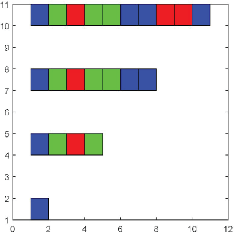
Introduction. — We propose a model of an excitable medium that can generate waves of a new kind. These waves consist of interacting narrow fronts. The evolution of the coordinates that define the localization of those fronts, is governed by a dynamical system. The key point is that we can control the attractors of these dynamical systems by positional information stored in spatially distributed initial data and by the choice of a few of parameters. These attractors may be chaotic and of high dimension. We show that this effect has important biological consequences. As an example, we consider applications to morphogenesis, in particular, to cell differentiation problems. We resolve the cell pattern generation problem: imagine an arbitrary string of cells of different types located along the -axis (this might model -organisms, like a worm, or a segmented embryo, see Fig. 1). The cell pattern can be generated by our excitable medium, and we present an algorithm for how to do so.
To better understand our approach to the cell differentiation problem in more detail, recall two fundamental biological concepts. An organism can be represented as a pattern consisting of different cells (see Fig. 1). The cells are “specialized”, i.e., each type of cell performs a unique and special function and each of the order of different types of cells in multicellular organisms has different structures, sizes, shapes, and functions. The famous Turing instability approach (Turing 1952) allows us to obtain periodical layered patterns, such as zebra stripes, however, we would like to explain more complicated observed structures. To this end, the concept of positional information was proposed by Wolpert (Wolpert et al. 2002). Both approaches, Turing’s and Wolpert’s, assume that morphogens, special reagents, can change cell states.
Our new idea is that the waves with complex evolving fronts can perform cell differentiation in a dynamical way. This allows us to create any pattern not just periodic ones. The waves transfer a family of morphogenes, which change the cell states and produce cell differentiation. In contrast with Wolpert’s gradient model, the wave act at long distances and can transfer dynamical information contained in an attractor.
The main idea of the pattern generation mechanism is as follows. We restrict ourselves to one-dimensional layered patterns (a generalization to multidimensional cases will be presented in future papers). Consider the pattern shown on Figure 1. That pattern can be considered as a string of cell types (blue, green, red). Our aim is to create any such string. Note that a universal Turing machine (UTM) may print any string. A UTM includes a head and a tape, the states of the head form a finite set. The head moves along the tape and prints symbols. Our medium generates waves, which move along the -axis, and prints cells of different types. The type choice depends on the state of the wave front, defined by a chaotic hyperbolic dynamics. Here we use the beautiful idea from C. Moore Moore 1990; Moore 1991 on simulation of TM’s by chaotic dynamical systems. It is based on so-called Bernoulli shifts, chaotic dynamics can be encoded as a shift on a discrete set of symbols. So, the states of the waves can be encoded by a finite partition of all possible morphogen states. We present two variants of patterning algorithms, the first gives us a rigorous method to resolve any problems of pattern generation, and the second is a simplified variant that works well in numerical simulations.
These results show that there are media that function as analogs of UTM’s. A UTM can make all computations, which can be done by other TM’s, and so, UTM’s generate all possible string outputs when we vary their input. In our case, we have a fixed (up to a few parameters to adjust) spatially extended system, which, depending on initial data, generates all possible layered cell patterns. Note that UTM’s admit a short description Rogozhin 1996.
So, our results show that simple mechanochemical systems can serve as Universal Generators of spatio-temporal patterns (UPG). Thus they can be considered as analogs of UTMs. A UTM obtains a program as an input and performs computations prescribed by that program. In our case, the input of our UPG is determined by spatially distributed initial data localized in a narrow domain.
Cell differentiation waves are proposed in (Gordon and Brodland 1987), see also (Gordon and Gordon 2016). Cell killer waves are found in (Cheng and Ferrell 2018). Apoptosis (programmed cell death) propagates through the cytoplasm as self-regenerating trigger waves, which spread without slowing down or petering out. Cell differentiation waves in Drosophila morphogenesis are found experimentally and investigated in (Bailles et al. 2019), where, moreover, a conceptual mathematical model is proposed, which involves reaction and diffusion, and exploits mechano-chemical effects, where chemical reaction terms are linear and quadratic. The model (Bailles et al. 2019) describes the time evolution of concentrations of free Fog ligand, bound-receptor Fog, and MyoII protein.
Waves of cell differentiation are studied experimentally in (Chhabra et al. 2019), where it is indicated that signaling patterns may be dynamic, and cells may use various strategies to interpret these dynamics. To investigate this dynamical mechanism, in (Chhabra et al. 2019) WNT and Nodal signaling pathways are studied. BMP signaling triggers waves of WNT and NODAL signaling activities, which move toward the colony center at a constant rate. It is shown that it is inconsistent with reaction-diffusion-based Turing models, suggesting that neither WNT nor NODAL forms a stable spatial gradient of signaling activity. So, the experiments and theoretical models show that, at least in certain situations, the morphogenesis proceeds with the help of waves, while the celebrated Turing instability does not work Chhabra et al. 2019. However, the pathways involved in the wave dynamics are extremely intricate.
Similarly to Chhabra et al. 2019; Bailles et al. 2019, in our model we use reaction and diffusion, and also linear elastic waves but we also implement into our model the scalar Ginzburg-Landau (GL) equation with a small gradient term. That equation describes bistability, and spontaneous layered patterning. The GL equation simulates a trigger mechanism, which in real biological systems is generated by positive feedback loops in gene regulation networks (those loops are detected in killer waves (Cheng and Ferrell 2018)). This extends possibilities in a formidable way: spontaneous symmetry breaking creates complicated dynamical information and transfers that information through active media.
Let us outline our model. It consists of three equations. The first equation is a weakly perturbed Ginzburg-Landau (GL) equation for a scalar order parameter . We suppose that the coefficient at the gradient term in the corresponding energy is small. It is well known that the non-perturbed GL equation has asymptotical solutions describing kink chains, where -th kink is localized at . Kinks are narrow topological defects (of width ) with the charge describing a symmetry breaking: a separation of the entire domain on subdomains along -axis, where . Note that the direct interaction between kinks is exponentially small and therefore such a solution is correct within an exponentially long time while kinks are separated Carr and Pego 1989. Furthermore, we use a simple perturbation, which makes the kink chain move as a whole at a low constant speed . The following equation describes the reaction-diffusion dynamics of -reagent, where the order parameter is involved. Reagent diffuses fast. The kinks interact with the fast reagent and the reagent acts on , which that produces feedback and non-local non-direct kink interaction. We show that under an appropriate choice of system parameters the dynamics of the kink coordinates can be described by the Hopfield system with continuous-time and non-symmetric interactions. It is well known that such Hopfield systems exhibit a remarkable universality property Vakulenko 2000: they can generate any structurally stable (hyperbolic) dynamics. Such dynamics may be chaotic (the best known examples are given by Anosov flows and Smale horseshoes Ruelle and Dewitt-Morette 1990; Katok and Hasselblatt 1997). Following Moore 1990; Moore 1991 we can use this chaos to simulate Turing machines and we apply it to program pattern formation.
We would like to note that curved chaotic fronts can also be described by the Kuramoto-Sivashinsky (KS) equation Sivashinsky 1980; Kuramoto 1978. In our case, a physical mechanism of the chaos generation is absolutely different: instead of curvature effects, we use a non-local kink interaction via coupling with a fast diffusing reagent. While most of the known results for the KS model are numerical (see, for example, (Pathak et al. 2018)), our model is analytically tractable and there is an algorithm to control the wave front dynamics.
The model and its properties. — The model consists of a reaction-diffusion part, a hyperbolic equation, and a scalar Ginzburg-Landau equation for an order parameter :
| (1) |
| (2) |
| (3) |
Here and are small parameters, and are unknown functions defined on , is the strip . Eq. (3) for can describe elastic (mechanical) effects, and the deformation affects via a quadratic nonlinearity. To simplify the problem, and bearing in mind further the propagation of waves, we set the periodic boundary conditions
| (4) |
At the boundaries and we set the zero Dirichlet conditions for :
| (5) |
and the zero Neumann condition for
| (6) |
The initial conditions are given by smooth functions and , for example,
| (7) |
and similarly for . The function plays a key role in long time behaviour control.
The key difference between this system and the model of Bailles et al. 2019 is the presence of the GL equation (1), which describes phase transitions and layered patterning. So, we can take into account basic mechanical, chemical, and physical effects, and we think that this model is the most efficient among all those providing the effects described in the manuscript. Note that our model is two-dimensional that is important for the control of large time dynamics. To obtain analogous results in one-dimensional case, we have to use a number of reagents replacing a single eq. (1) by a reaction-diffusion system.
Asymptotic solutions and mechanism of chaos onset.— In this model, chaos appears as a result of a non-local kink interaction. For each integer and sufficiently small and there exist solutions describing interaction of kinks. The -component of these solutions are perturbed -periodic in kink chains consisting of kinks well localized at points , where are slowly evolving in time relative kink coordinates. Analogous kink solutions for (1) are described first in (Carr and Pego 1989). Such solutions are metastable and exist while kinks are well separated, and the kink existence time interval is of the order (Carr and Pego 1989). So, our solutions have the form
| (8) |
| (9) |
where are small corrections with respect to the main terms and . The following relation is important:
| (10) |
where are smooth functions. The function defines a response of -reagent to the excitement generated by -th kink. In turn, the -reagent acts on kinks via the small perturbation in Eq. (1). So, we obtain a feedback and a non-local nonlinear interaction between the kinks, which is much stronger than exponentially small interactions between nearby kinks. For an appropriate choice of the small parameters , and the initial data one can show that, up to small corrections, the time evolution of kink coordinates is governed by the time continuous Hopfield system
| (11) |
where is a smooth sigmoidal function, the matrix with entries defines an interaction between , are thresholds and . The form of this system depends on parameters , . The matrix and are linear functionals of initial data . The key point is that by variation of we can obtain any given (not necessarily symmetric, see SM).
The Hopfield systems with general non-symmetric interactions enjoy remarkable properties. We know that multilayered perceptions can approximate any output (Theorem on Universal Approximation). By that basic result, one can show that the Hopfield system has the property of Universal dynamical approximation. Namely, they can simulate, within any prescribed accuracy, any finite-dimensional dynamical systems (see (Vakulenko 2000; Vakulenko et al. 2016) and SM). This simulation works via hidden slow variables, which appear in the Hopfield dynamics under an appropriate choice of . Then, that matrix defines an interaction between slow and fast variables. As is typical, in such slow-fast systems, the slow variable dynamics captures the entire system’s long-time behavior. By parameter we can completely control the slow dynamics (up to small smooth corrections).
For example, suppose we would like to simulate the Lorenz dynamics within accuracy . Then we can adjust parameter in such a way that (11) becomes a slow-fast system, and the slow part dynamics is defined by the -perturbed Lorenz system. This simulation holds, in general, on large time intervals, but if the attractor of the prescribed system is structurally stable (for example, hyperbolic), i.e., does not change its topology under sufficiently small and smooth perturbations, then for small -the simulating Hopfield dynamics is the same (up to topological equivalency of trajectories). Roughly speaking this means that system (11) can simulate all hyperbolic dynamics, for more precise formulation see (Vakulenko 2000) and SM). These facts lead to the results described in the coming section. Note that a connection between the neural network Hopfield model and reaction-diffusion systems was first discovered in (Edwards 1996), see (Vakulenko 2000) for a rigorous proof.
Formation of cell patterns. — To describe patterns consisting of differentiated cells and cell differentiation via the reagent , we use the model, which follows the biological ideas (Turing 1952; Wolpert et al. 2002) outlined in the introduction. Consider, for simplicity, two cell types, say, red and blue cells. We encode them by and , respectively (the generalization for a larger number of cell types is quite straightforward). We assume that cells occupy strips of the same small length forming a layered pattern along the -axis. We thus have equidistant layers. The output cell pattern can be considered as a binary string : , where is either , or . We also introduce a state . The state zero corresponds to cells that are not yet differentiated.
Next, we describe how the cell pattern can be produced in our model. The cell pattern is a result of terminal differentiation which goes by morphogens. Suppose that the is a morphogen. It is natural to assume that cells interpret morphogen signals by averaging in space and time. For simplicity, we assume that this interpretation goes through linear convolution operators, which act on the -pattern (see SM). So, the cell obtains information about kink coordinates at the moments when the kinks reach the cell. Let us consider how this information can be used. The range of all possible values will be denoted by . We introduce the partition of consisting of disjoint subsets , such that their union is and each subset has an open interior. This partition has a simple meaning: we encode the continual space of wave states by a discrete code. The set corresponds to non-differentiated cells, the set with corresponds to cells of -th type. We encode kink states by functions . The coding function takes the value if . Let be the asymptotic kink solution. Then the output string can be defined as follows: -th element of the string is , if , where is the moment when kink chain wave reaches -th cell. This construction replaces thresholds in the Wolpert positional information approach, but in our case, this information is transferred in the cells by waves instead of gradients. We refer to as wave cell differentiation operator, for more details see SM.
Note that at the moment the corresponding cell accepts -th state and does not change its type anymore. We assume here the biological fact that typical cells do not change their cell types after terminal differentiation when they acquire their specialized type. At all cells are in an indefinite state .
Main results.—Concluding the ideas presented above we formulate the following statements.
On dynamical complexity: Kink dynamics of our model has the property of universal dynamical approximation.
This means that when we vary the model parameters, initial data and the kink number, kink coordinate dynamics can generate all possible kinds of structurally stable large time behavior (up to topological equivalency). Since hyperbolic dynamics is persistent (Katok and Hasselblatt 1997), kink motions generate all hyperbolic dynamics. Hyperbolic dynamics may be chaotic (Katok and Hasselblatt 1997; Ruelle and Dewitt-Morette 1990), and further, we show how hyperbolic chaos generates all possible layered patterns. It can be done by an algorithm, which allows us to obtain a prescribed cell pattern.
The next statement unwraps the main problem of cell pattern formation.
On the cell pattern generation problem: Let be a prescribed string of cell types, . To find parameters and initial data such that the corresponding solution of Initial Boundary Value Problem (IBVP) defined by eqs. (1)-(3) and conditions (6)-(7) satisfies
| (12) |
where is the wave cell differentiation operator.
The last statement can be formulated as follows.
The pattern generation problem has a solution.
We describe algorithms to resolve this problem in the coming section.
Pattern generation.— We propose algorithms to solve the pattern generation problems based on celebrated results of dynamical system theory on hyperbolic sets, in particular, the existence of Markov partitions that implies the correspondence between maps on invariant hyperbolic sets and Bernoulli shifts (Katok and Hasselblatt 1997; Moore 1990; Moore 1991). The idea of the algorithm can be outlined as follows. We first encode a cell pattern as a string in an alphabet of cell types. The algorithm input is then a string of symbols from (see Fig. 1). We would like to produce such a string. We know that a UTM can print that string: the UTM head moves along the tape and prints. Similarly, our wave moves along the -axis and prints different cells. Although states of that wave lie in a bounded domain of , we can make a partition of that domain to encode the wave states. Then the wave becomes an analog of the UTM head. Here we use Bernoulli shifts and the same idea that allows realizing TM’s by dynamical systems, see SM for more details.
Note that the algorithm is based on the well-known biological fact that cells (except for stem cells) are not capable of further differentiation. When a wave comes to an area occupied by a cell, it changes its type (depending on the amplitude of the wave), that is, it makes differentiation and after that, the cell no longer changes.
So, we conclude that there is a universal reaction-diffusion system, which can produce any cell phenotypes depending on initial data and a few parameters, i.e., we can obtain a needed final (terminal) phenotype.
The chaotic hyperbolic attractor can be taken, in principle, in an arbitrary way, however, it is natural to take a low dimensional one. The choice of the Markov partition depends on the coding scheme, which we use for cell types.
Our chaotic attractors generate strings within time intervals, but by waves described above, we can obtain a generation along the -axis.
Numerical example and simplified algorithm.— As an example of the algorithm application, let us consider how to create the pattern in Fig. 1. Numerical simulations show that the sophisticated algorithm stated above can be strongly simplified. We can, instead of the Markov partitions, use almost arbitrary partitions of phase space on disjoint subsets. We consider first how to generate layered pattern like the famous French flag by waves instead of gradients. Consider the pattern in Fig. 1 consisting of layers: blue, green, red, and again green. Suppose for simplicity that all layers of the cell pattern have the same width then the string corresponding to that pattern is . We take the Lorenz system for variables with the standard choice of parameters to produce a chaotic attractor . Further, we find the Hopfield system such that the kink coordinates evolve according to weakly perturbed Lorenz system, .
Let us introduce , , and . Then we take the partition , and . Then one can check numerically that there exist points on the Lorenz attractor and such that , , and . Here correspond to blue, white and red cells, respectively. The partition of -space, which define cell differentiation, is formed by ranges of under the map . So, we obtain the layered aperiodic -pattern consisting of four layers (see Fig. 1, the second row from bottom). The same construction allows us to obtain more complicated patterns, for example, consisting of five and more layers. Note one can take other sets so the choice of the partition is almost arbitrary. However, the longer the cell pattern becomes, the smaller the set of starting points will be, and thus it is more difficult to find that set.
This simplified variant of the algorithm can be analytically explained under the assumption that the dynamics on the attractor is strongly mixing (see SM, subsect. II.6.2). Moreover, this variant is robust with respect to the choice of partitions. However, the sophisticated algorithm with Poincaré map has an advantage: by the Bernoulli shifts and the Markov partitions, we can find the set of initial data and the corresponding initial kink coordinates in an explicit way. The pattern generation by the simplified algorithm can be observed in a video, see (https://youtu.be/4frNmeqkhgE 2021).
Conclusions. — A key component for achieving functionally stable multicellular structures is a physical embodiment. Any relevant model of the evolution of multicellular organisms should actually take into account basic physical mechanisms. It is shown that there exists a simple physical model defined by three equations with quadratic and cubic nonlinearities which create the chaotic waves of a new type. These waves have fronts, which can be interpreted as ”moving” attractors and they can transfer information since dynamical systems with a complicated behavior can simulate all Turing machines (Moore 1990; Moore 1991). Such waves can transfer information in space, for example, innovations. Following (Collinet and Lecuit 2021) one can say that excitable media can create programmed and self-organized flows of information. Propagation of complicated information, which may seem to be the exclusive prerogative of human society is possible in simple physical media. These results can be applied, in particular, to cell differentiation problems. New pattern formation mechanism described here can produce any target cell patterns.
Physical processes mobilized by genes can establish morphological templates. Most animal body plans and morphological motifs arose between 500 and 700 million years ago, during relatively brief periods of innovation. The genes, whose products control morphogenesis and pattern formation, were present in the unicellular ancestors of the animals; billion years of evolution failed to generate substantial additional morphological novelty. The work (Newman 2012) reconciles these facts by proposing that chemically and mechanically active media can create the main motifs of animal forms. Our results support this concept of physical determinism in development. We also think that the proposed pattern generation mechanism can appear in other applications, for example, in ecology and economics.
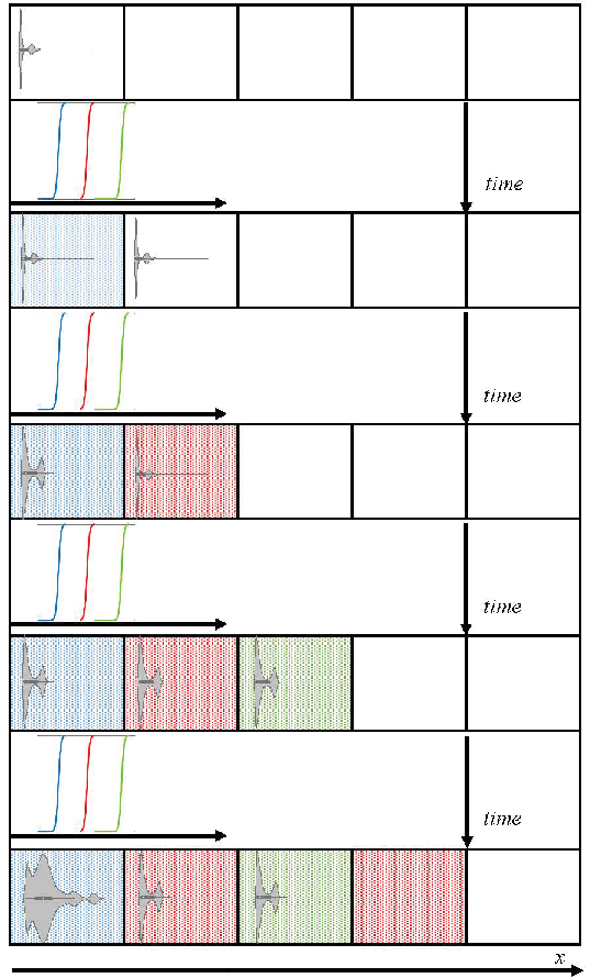
The active media that generate complex waves are simple and the generation mechanism involves fundamental physical and chemical effects of physics. A few genes is sufficient to correctly encode that mechanism. Therefore, it is natural to expect that such media could appear as a result of biological evolution. One can imagine, for example, such a model (see Fig. 2). Consider a cell colony that must adapt to a new environment and develops products necessary for survival. It is clear that a colony, where it is possible to transfer complex adaptive innovations from one cell to another, has a clear selective advantage. This transmission can be done by means of the waves, studied in this paper, and these waves can not only transmit simple information, but they can also transfer complex behavior (which can be described by an attractor or a Turing machine, or a neural network with associative memory), similarly to human society.
Acknowledgments.— S. V. and J. R. are supported by the grant of National Institutes of Health (NIH) 2R01 OD010936. IS gratefully acknowledges support from the Division Of Physics at the U.S. National Science Foundation (NSF) through Grant PHY-2102906.
References
- Turing (1952) A. Turing, Phil. Trans. Roy. Soc. B 237, 37 (1952).
- Wolpert et al. (2002) L. Wolpert, C. Tickle, and T. Jessell, Principles of development (Oxford University Press, 2002).
- Moore (1990) C. Moore, Phys. Rev. Lett 64, 2354 (1990).
- Moore (1991) C. Moore, Nonlinearity 4, 199 (1991).
- Rogozhin (1996) Y. Rogozhin, Theoretical Computer Science 168, 215 (1996).
- Gordon and Brodland (1987) R. Gordon and G. W. Brodland, Gell Biophys. 11, 177 (1987).
- Gordon and Gordon (2016) N. K. Gordon and R. Gordon, Theoretical Biology and Medical Modelling 13 (2016).
- Cheng and Ferrell (2018) X. Cheng and J. E. Ferrell, ArXiv arXiv:1806.04138v1 [q-bio.TO] (2018).
- Bailles et al. (2019) A. Bailles, C. Collinet, J. Philippe, P. Lenne, E. Munro, and T. Lecuit, Nature 572, 467 (2019).
- Chhabra et al. (2019) S. Chhabra, L. Liu, R. Goh, X. Kong, and A. Warmflash, PLOS Biology 17, e3000498 (2019).
- Carr and Pego (1989) J. Carr and R. Pego, Comm. on Pure and Applied Math. 42, 523 (1989).
- Vakulenko (2000) S. Vakulenko, Advances in Differential Equations 5, 1139 (2000).
- Ruelle and Dewitt-Morette (1990) D. Ruelle and C. Dewitt-Morette, Physics Today (1990).
- Katok and Hasselblatt (1997) A. Katok and B. Hasselblatt, Introduction to the modern theory of dynamical systems (Cambridge University Press, 1997).
- Sivashinsky (1980) G. S. Sivashinsky, SIAM Journal on Applied Mathematics 39, 67 (1980).
- Kuramoto (1978) Y. Kuramoto, Progress of Theoretical Physics Supplement 64, 346 (1978).
- Pathak et al. (2018) J. Pathak, B. Hunt, M. Girvan, Z. Lu, and E. Ott, Phys. Rev. Lett. 120, 024102 (2018).
- Vakulenko et al. (2016) S. Vakulenko, I. Morozov, and O. Radulescu, Nonlinearity 29, 2327 (2016).
- Edwards (1996) R. Edwards, Mathematical methods in the applied sciences 19, 651 (1996).
- https://youtu.be/4frNmeqkhgE (2021) https://youtu.be/4frNmeqkhgE, Video (2021).
- Collinet and Lecuit (2021) C. Collinet and T. Lecuit, Nat. Rev. Mol. Cell. Biol https://doi.org/10.1038/s41580-020-00318-6 (2021).
- Newman (2012) S. Newman, Science 338, 217 (2012).
- Vakulenko and Volpert (2001) S. Vakulenko and V. Volpert, Nonlinear Analysis. TMA 46, 757 (2001).
- Vakulenko (2018) S. Vakulenko, Journ. Dyn. Diff. Equat. 30, 175 (2018).
- Smale (1967a) S. Smale, Bull. Amer. Math. Soc. 73, 747 (1967a).
- Metzger (2000) R. J. Metzger, Annales de l’Institut Henri Poincaré 17, 247 (2000).
- Young (2002) L. S. Young, Journal of Statistical Physics 108, 733 (2002).
- Arnold et al. (1994) V. I. Arnold, V. S. Afrajmovich, Y. S. Il’yashenko, and L. P. Shil’nikov, Dynamical systems V, Bifurcation Theory and Catastrophe Theory (Encyclopedia of Mathematics, Springer Verlag, 1994).
- Poláčik (1991) P. Poláčik, Journal of Differential Equations 89, 244 (1991).
- Poláčik (1995) P. Poláčik, Journal of Differential Equations 119, 24 (1995).
- Vakulenko (2021) S. Vakulenko, Journ. Dyn. Diff. Equat. 33, 303–343 (2021).
- Smale (1967b) S. Smale, Bull. Amer. Math. Soc. 73, 747 (1967b).
- Henry (1981) D. Henry, Geometric theory of semilinear parabolic equations, Vol. 840 (Springer-Verlag, Berlin, 1981).
- (34) If we approximate a dynamics within a finite time interval, the assumption on structural stability can be removed.
I Supplementary Material
II Asymptotic solutions to system (1)-(3) describing complex waves
II.1 Kink chains
Let us describe kink chains following (Carr and Pego 1989). Let first . Let , be coordinates of the kinks in the interval . We suppose that . Let and . We assume
| (13) |
i.e., maximal and minimal distance between kinks are small. The minimal distance is much more than the characteristic diffusion length and the maximal one is much less than the cell size . We need these assumptions to have an asymptotics solution in the form of a kink chain and also to construct a simple cell pattern generation operator (see subsect. II.6).
The kink chains can be obtained by -periodical in functions , which have the following form. Inside narrow intervals , has the form , where are topological charges and . Outside of intervals the function is exponentially close to and this function is a smooth function of . For we have a set of solutions of (1), which have the form , where is a small correction and the kink coordinates evolve in time exponentially slowly: (Carr and Pego 1989). These solutions are correct while . Time evolution of is a result of exponentially weak direct kink interaction. For we obtain the kink chain travelling with a constant speed : .
In the coming subsection we consider the case , where we have more complicated equations for . In this case there is a non-direct and non-local kink interaction via coupling with -reagent.
II.2 Equations for kink coordinates
Solution of eq. (3) has the form . We substitute into eqs.(1), (2) and make variable change (further we omit tilde in notation). Then we obtain the following system
| (14) |
| (15) |
Further we find asymptotic solutions of that system under the following assumptions to the small parameters:
Assumptions to and
Let be small enough and
| (16) |
where are uniform in .
The main idea in choice of is to conserve the planar structure of the kink fronts ( otherwise it is impossible to describe kink chains by coordinates , and it is necessary to take into account the front curvature). The parameter should be small as well in order to obtain quasistationary solutions of eq. (15). The condition is neccesary to ensure domination of non-local kink interaction via -reagent with respect to direct kink one.
The subsequent statement follows works (Carr and Pego 1989; Vakulenko 2000; Vakulenko and Volpert 2001; Vakulenko 2018) with small modifications. Our first goal is to derive equations for . Eqs. for can be derived by a standard perturbation approach for small (see, for example, (Carr and Pego 1989; Vakulenko and Volpert 2001)). For sufficiently small one has
| (17) |
where is the kink chain (see above) and is a correction. Then the time evolution of is governed by the system
| (18) |
where
| (19) |
and small corrections are uniformly bounded
where , are uniform in as .
To explain equations (18) and (19), let us remind the construction from (Vakulenko and Volpert 2001), which is the well known Lyapunov-Schmidt factorization. To obtain the dynamical equations for , we impose the condition
| (20) |
for each . These equations define uniquely for small and bounded . For the correction we obtain
| (21) |
where is the linear operator defined by
| (22) |
and
The spectrum of the operator is well studied (Carr and Pego 1989). Note that is a self-adjoint operator of Schrödinger type, which has a kernel consisting of eigenfunctions associated with kink Goldstone modes, which describe kink shifts.
Let , where the normalizing constants provide . Note that equal up to exponentially small corrections.
We use the standard notation
We need the following Lemma (see (Vakulenko 2018)).
Lemma 1For such that
one has
| (23) |
and if for all then
| (24) |
where all constants are uniform in as .
For a proof see (Vakulenko 2018).
So, the spectrum of consists of exponentially small eigenvalues and all the remaining spectrum of lies in the interval , where does not depend on . This property implies the stability of the kink solutions on exponentially large intervals and allow us to solve eq. (21). It can be done by the standard perturbative methods because these equations involve weak nonlinearities while the linear part is stable due to condition (20), which also implies dynamical equations (18) for .
II.3 Quasistationary solutions of (2)
Let us turn now to equation (2) for . This equation is linear with respect to both and , is a sum , where is small. The function depends on time via slow variable and does not depend on explicitly. Therefore, we can solve that equation by a simple idea: we can freeze in eq. (2) assuming that is just a parameter. Thus the main contribution to is given by the function satisfying the equation
We obtain
| (26) |
| (27) |
For small the function is a good approximation of -function (up to a constant uniform in ). Moreover, it is clear then that in eqs. (27) can be replaced by . Let us denote by the Green function of the one-dimensional boundary value problem satisfying the equation
and the -periodical boundary conditions in . Then we resolve (27) by the Fourier method that gives
| (28) |
where and are the Fourier coefficients of :
where are positive integers.
II.4 Hopfield system
Using relations (26), eqs. (18), (19), and removing small terms, we obtain evolution equations for kink coordinates :
| (29) |
where
| (30) |
Our goal is to reduce this system to the Hopfield one. It can be done by a special choice of , or, that is equivalent, of . First we substitute formula (28) into (30). Then we have
| (31) |
where
The main idea to simplify the formula (31) for is as follows. Suppose that the kinks oscillate at certain fixed points , i.e.,
| (32) |
where are new unknowns. Suppose temporarily that as , where is a small parameter. (this assumption will be justified later). We can achieve such behaviour of solutions under a special choice of . Positions of points may be arbitrary but the condition
must be satisfied.
Namely, we set
| (33) |
| (34) |
| (35) |
where is a smooth sigmoidal function, for example,
and where are unknown coefficients, which must be matched appropriately.
We obtain then
| (36) |
Then we can simplify (36) that gives (up to terms of the order )
| (37) |
Further we use the following lemma.
Lemma II. For each matrix with entries there exist a number and coefficients such that
| (38) |
Proof. For unknown we have a system of linear algebraic equations. For large we have asymtotics
| (39) |
for . Hence for sufficiently large the matrix of our linear algebraic system contains a non-degenerate Vandermond matrix as a submatrix thus that linear algebraic system is resolvable.
Using this lemma, we can choose and such that take the form
| (40) |
where .
II.5 Control of dynamics for Hopfield system
Using (40) we obtain the following system for new variables :
| (41) |
It is easy to show that system (41) has a compact attractor. In fact, thus that system implies the inequalities
where . These differential inequalities lead to the estimate
The last estimate shows that system (41) has an absorbing set , thus it is dissipative and has a compact attractor. This result justifies our hypothesis on smallness of kink oscillations at points and the transformation of general system (29) to the Hopfield system (41).
The following claim is proved in (Vakulenko 2000).
Theorem I. Dynamics defined by system (41) generates all finite dimensional hyperbolic dynamics (up to orbital topological equivalency) by variations of parameters and .
II.6 Morphogenesis algorithms by waves and physical effects
Let be a finite set of cell types. We assume that -th cell occupies a subdomain centered at , where . We thus have equidistant cells, . The output cell pattern can be considered as a string in the alphabet : , where is the number of cells. We suppose that condition (13) holds, which means that all kink chain can enter in the cell.
Let us describe now how the cell pattern can be produced in our model. We follow classical ideas (Turing 1952; Wolpert et al. 2002). The cell pattern is a result of terminal differentiation, which goes by morphogens. Suppose that is a morphogen. Following the positional information concept, one can assume that differentiation starts, when the concentration of at the cell center is large enough, say, , where is small. Suppose that initial coordinates of all the kinks satisfies and the topological charge of the leading kink with the coordinate is . Then for the moment one has (it is a moment when the leading kink approaches the center of -th cell). It is well known that cells interpret morphogen signals by averaging in space and time. For simplicity, we consider linear averaging operators
| (42) |
where is a smooth weight function with the support . We have . Since for small the kink chain can be approximated by a piecewise-constant functions with breaks at and kinks oscillate at points , relation (42) leads to
| (43) |
where are coefficients. Thus we conclude that the cell can obtain an information about coordinates at the moment , when the waves reach the cell, via the linear combinations of the kink positions.
Let us consider how this information can used. The range of all possible values will be denoted by . We introduce the partition of consisting of subsets , with disjoint open interiors such that their union is . The set corresponds to non-differentiated cells, the set with corresponds to cells of -th type. We encode kink states by functions . The function takes the value if .
Then the output string of cell types can be defined as follows: -th element of the string is , if , where is the moment when the waves reach -th cell (see above). This construction replaces thresholds in the Wolpert positional information approach, but in our case this information is transferred in the cells by waves instead of gradients. Note that at the moment the corresponding cell accepts -th state and does not change its type anymore. We use here the biological fact that usually cells do not change their cell types after terminal differentiation, when they acquire their specialized type.
II.6.1 Algorithm using Markov partitions and Bernoulli shift
An algorithm to solve the pattern generation problems is based on celebrated results of dynamical system theory on hyperbolic sets, its persistence, existence of Markov partitions and a connection between Bernoulli shifts and maps on invariant hyperbolic sets (Katok and Hasselblatt 1997; Moore 1990; Moore 1991). Let us consider a smooth map , where lies on a smooth compact finite dimensional manifold (for example, torus). Suppose this map defines a dynamical system with discrete time: , which has a hyperbolic invariant set . Dynamics on can be described by a Markov partition consisting of a family of sets (Moore 1991). Iterations is equivalent to a Bernoulli shift map defined on the set of all such two-sided sequences : (Moore 1991). Each points on the hyperbolic set has an ”address”, which is a two-sided sequence , , and that addresses predetermines the point fate under dynamics (Moore 1991). Nonetheless such shift dynamics may be chaotic: a small error in initial data can lead to an exponential divergence in subsequent iterations, to predict the system steps in the future, we need to know roughly symbols of the initial sequence.
To use these ideas, we first encode cell pattern as a string in an alphabet of cell types. The algorithm input is then a string of symbols from . The algorithm steps are as follows.
- 1.
We find a discrete time dynamical system with an appropriate hyperbolic attractor, which has a Markov partition consisting of subsets . For the alphabet (or ) one can use the famous map generating a hyperbolic chaotic behaviour, so-called Arnold’s cat map defined on the torus . Let us define the matrix by
and let us set . The map is conjugate to a Bernoulli shift and the corresponding Markov partition consists of two rectangles ;
- 2.
By a suspension (see Smale, (Smale 1967a)) we find an integer and a smooth vector field such that the corresponding flow defined by the system
(44) on a compact domain with a smooth boundary has a Poincaré section and the corresponding Poincaré map is the map described at the previous step;
- 3.
Using equivalency between iterations and the Bernoulli shifts we find a subset consisting of initial data for (44) such that the -th iteration of enters for the subset for ;
- 4.
Let be a constant such that the Poincaré map persists under perturbations of the vector field , which -small in -norm. Such a constant exists due to properties of hyperbolic dynamics (see Appendix and (Katok and Hasselblatt 1997; Ruelle and Dewitt-Morette 1990)). We realize the vector field by a Hopfield system (11) within accuracy (about realisations see Appendix); then dynamics of -states is defined by the map , where evolves according to -perturbed equation (44);
- 5.
we define the sets in space as ranges of rectangles under the maps ;
- 6.
- 7.
we release a kink chain wave at a suitable speed .
The last point of the algorithm is based on the well known biological fact that cells (except for stem cells) are not capable of further differentiation. When a wave comes to an area occupied by a cell, it changes its type (depending on the amplitude of the wave), that is, it makes differentiation and after that the cell no longer changes.
Note that if is the Arnold cat map, then one can take . It follows from Whitney theorem. The strong Whitney embedding theorem states that any smooth -dimensional manifold ( Hausdorff and second-countable) can be smoothly can be embedded in the -dimensional Euclidian space. The Smale suspension gives us -dimensional manifold, where a flow generates the Arnold map as a Poincaré map. This manifold can be embedded in .
II.6.2 Simplified algorithm
Let eq. (44) define a smooth dynamical system defined on a ball in with an attractor , which has an invariant measure defined on (for axiom A attractors and Anosov diffeomeorphisms such measures exist and they are well studied, they are called Sinai–Ruelle–Bowen (SRB) measures (Metzger 2000; Young 2002)). Suppose that the flow generated by system (44) has the strong mixing property, i.e.
for two measurable sets . Let be a subset of non-zero -measure on and be a small open neighborhood of in . Let be a fixed partition of and be a fixed positive integer. Then the mixing property implies that if is large enough all the following intersections are non-empty:
In fact, according to the strong mixing property . Moreover, it is easy to see that
This shows that for any finite sequence , of there is an open (possibly small) set of initial points such that
Let us note that the sophisticated algorithm with Poincaré map has an advantage with respect to the simplified one: by the Bernoulli shifts and the Markov partitions, we can find the set of initial data in an explicit way. For simplified algorithm it can be done numerically. We have checked it for the Lorenz system for .
III Appendix
III.1 Realisation of vector fields (RVF)
The main technical tool in proving attractor complexity for partial differential equations and systems is realization vector field (RVF) method based, in particular, on structural stability ideas. It is based on a classical center manifold technique and on the well known idea that any -dimensional dynamics can bifurcate from an equilibrium with - zero eigenvalues if the number of bifurcation parameters is large enough. Such approach was used for finite dimensional systems (see (Arnold et al. 1994)), but it can be extended on infinite dimensional evolution equations. This RVF approach is developed by first P. Poláčik to prove existence of non-trivial large time behaviour for quasilinear parabolic equations (see (Poláčik 1991; Poláčik 1995)) and developed in (Vakulenko 2000; Vakulenko 2018) for reaction-diffusion systems, in (Vakulenko et al. 2016) for neural networks and in (Vakulenko 2021) for weakly compressible Navier-Stokes equations.
In our model, , where is the number of kinks, eigenvalues are exponentially close to zero and the initial data plays the role of the main bifurcation parameter, i.e., the bifurcation parameter is infinite dimensional.
III.1.1 Structural stability
Recall the basic concept of structural stability introduced by A. Andronov and S. Pontryagin in 1937. Consider a smooth vector field on compact domain of with a smooth boundary (or on a compact smooth manifold of dimension ). Assume that and consider all -small perturbations such that
| (45) |
Consider systems of differential equations and and suppose that they define global semiflows and on . The system is called structurally stable if there exists a such that if
then trajectories of semiflows and are orbitally topologically conjugate (there exists a homeomorphism, which maps trajectories of the first system into trajectories of the second one). Roughly speaking, the original system is structurally stable if any sufficiently small perturbations of that system conserve the topological structure of its trajectories, for example, the equilibrium point stays an equilibrium (maybe, slightly shifted with respect to the equilibrium of non-perturbed system), the perturbed cycle is again a cycle (maybe, slightly deformed and shifted).
Note that structurally stable dynamics may be, in a sense, ”chaotic”. There is a rather wide variation in different definitions of ”chaos”. We restrict ourselves hyperbolic chaotic sets. Chaotic (no periodic and no rest point) hyperbolic sets occur in some model systems (Smale 1967b; Ruelle and Dewitt-Morette 1990; Katok and Hasselblatt 1997).
III.2 RVF for evolution problems in Banach spaces
Let us consider a family of local semiflows in a fixed Banach space . Assume these semiflows depend on a parameter , where is another Banach space. Denote by the ball in , where and . For we will omit the radius , . Remind that a set is said to be locally invariant in an open set under a semiflow in if is a subset of and each trajectories of leaving simultaneously leaves . In this paper, all are tubular neighborhoods of the balls , which have small widths. Consider system of differential equations defined on the ball :
| (46) |
where
| (47) |
Assume the vector field is directed strictly inward at the boundary :
| (48) |
Then system (46) defines a global semiflow on . Let be a positive number.
Definition. (realization of vector fields) We say that the family of local semiflows realizes the vector field (dynamics (46)) with accuracy (briefly, - realizes), if there exists a parameter such that
(i) semiflow has a locally invariant in a open domain and locally attracting manifold diffeomorphic to the unit ball ;
(ii) this manifold is embedded into by a map
| (49) |
where ;
(iii) the restriction of the semiflow to is defined by the system of differential equations
| (50) |
where
| (51) |
Definition. Let be a set of vector fields , where each is defined on a ball , positive integers may be different. We say that the family of local semiflows realizes the family if for each and each the filed can be -realized by the family .
We say that the family of global semiflows has the property of universal dynamical approximation if that family realizes the set of all - smooth finite dimensional fields defined on all unit balls .
Many systems enjoy the property of universal dynamical approximation, for example, the Lotka-Volterra system with many species, the Hopfield system, a large class of reaction-diffusion systems and others.
III.3 Estimate of accuracy of asymptotic wave solutions
In this subsection, we estimate the accuracy of asymptotic solutions, which are correct under some restrictions to parameters and . We consider the IBVP defined by (14)-(15), boundary conditions (5), (4), (6) and initial data (7) assuming that initial data for lie in a narrow neighborhood of the kink chain . Then, by standard semigroup theory (Henry 1981), we are capable to prove the global existence of solutions for all and justify correctness of kink chain asymptotics. The statement mainly follows (Carr and Pego 1989; Vakulenko 2000; Vakulenko 2018).
III.3.1 Linear operator and projections
Let us consider the linear operator associated with the linear part of eq. (1) for and defined by (22). This operator depends on kink coordinates as a parameter, however, under condition (13) we can obtain estimates of its spectrum uniform in . Taking into account this fact, we omit a dependence on in notation.
Let us introduce the complementary projection operators defined on :
Let us formulated an auxiliary lemma.
Spectral Barrier Lemma. Let satisfy (13). Let and . Then for sufficiently small
| (52) |
This assertion is simply a reformulation of Lemma I by projection operators.
So, if we restrict the operator to functions orthogonal to all , then for that operator there exists a small spectral barrier of the order . In subsequent estimates this fact plays a key role. Moreover, constants , which appear in those estimates, are uniform in small parameters and .
III.3.2 Function spaces, norms and estimates
Let us introduce the inner scalar product in the space of -periodic in measurable functions defined on by
| (53) |
Let be the corresponding norm, i.e., . We denote by the Hilbert space of measurable functions defined on and - periodical in with bounded norms . We consider our IBVP problem in the space , i.e., and .
Let us introduce the fractional spaces (Henry 1981) defined by
where is the Laplace operator under the Dirichlet boundary conditions with a natural definition domain and . Here . Similarly,
where is the Laplace operator under the Neumann boundary conditions. We denote the product by .
Let us introduce the corresponding fractional spaces
with the norms
where . We use the well known estimate (Henry 1981)
| (54) |
where is a constant.
Let us prove first that our IBVP problem is well posed and defines a local semiflow. The proof is standard and follows (Henry 1981). We consider this problem in the Hilbert phase space . Let and . Our IBVP can be represented as an evolution equation (Henry 1981)
| (55) |
where is a self-adjoint operator in and
We use the Sobolev embeddings
| (56) |
that gives
These estimates show that is a -map from to and thus eq. (55) defines a local semiflow (Henry 1981).
III.3.3 Global existence
To establish existence of bounded solutions of our IBVP on infinite time interval , we need a priori estimates of weak norms, for example, and . They can be obtained in a standard way. Let us consider scalar products of the left and right hand sides of (1) with . Then under our boundary conditions eq. (1) implies the estimate
| (57) |
The same trick for eq.(2) gives
By integrating by parts in the last term and using that is a smooth and bounded function one obtains
Then the last differential inequality and the Poincaré inequality give
where . Thus we have the estimate :
| (58) |
We substitute this estimate into (57) that leads to
| (59) |
for . Consider the differential equation
We observe that if then for all . The differential equation for can be rewritten as
We observe then that , where is a solution of the linear differential equation
Therefore, we conclude that
and thus
| (60) |
By (58) this estimate implies
| (61) |
These estimates show that the norms of solutions are bounded on all bounded time intervals although these norms may slowly increase in . It implies, together with the estimates of the previous subsection, that solutions of our IBVP exist for all positive times and unique. Therefore, our IBVP generates the global semiflow.
In the coming subsections we show, in particular, that if the initial data for are close to the kink chain then the norms and stay bounded for all times while the mutual kink distances stay more than a small (for sufficiently small positive . If the kink coordinates oscillate at remaining in a small -neihborhood then and are bounded for all times. So, if the kink dynamics is governed by the Hopfield system then the norms and are bounded for all times.
III.3.4 Representation of solutions
III.3.5 Equations for , and
The estimates of this subsection hold under condition
To find equations for the slow variables and the fast ones we apply to (64) our projection operators that allows us to represent the system in the standard slow-fast form. This procedure gives
| (67) |
| (68) |
where
Using these equations we are capable to estimate and by the standard semigroup theory.
III.3.6 Estimates of and
Let , where may be large. All the subsequent estimates are uniform in under restrictions (16) to our small parameters. We introduce the norms
and for we write down simply etc.
Using the Spectral Barrier Lemma, we obtain, in a standard way by semigroup estimates (Henry 1981; Vakulenko 2018), that
where are constants uniform in . We note that
where the supremum of is taken over all and . We observe that . We also use the estimate (56) for that gives
| (69) |
Similarly,
| (70) |
The term can be estimated by (68). We find that
| (71) |
The system of inequalities (69), (70), (71) implies that under condition our evolution problem is weakly nonlinear and for small it can be resolved by standard contracting map principle (Henry 1981). We obtain
| (72) |
and
| (73) |
III.3.7 Locally invariant and locally attracting manifolds
Let us introduce the domains
| (74) |
Estimates established in the previous section hold under conditions
| (75) |
where is a positive constant. In general, it is impossible to guarantee that solutions of system of differential equations (68) satisfy an uniform estimate (74) for all . To overcome this difficulty, we perform the well known truncation procedure. Let be smooth increasing function of such that for and for . Consider equations
| (76) |
If solutions of the Cauchy problem for this system is defined for all for any and .
Lemma LIM (on existence of a locally invariant manifold) Let be an arbitrary positive number. Then for sufficiently small positive the semiflow, generated by (67), (65) and (76), has an invariant and locally attracting normally hyperbolic manifold of dimension defined by
| (77) |
| (78) |
where respectively, are maps from the ball , the number and the maps are bounded in -norm:
| (79) |
| (80) |
where are constants.
Proof. The proof uses the standard technique, see Theorem 6.1.7 from (Henry 1981) and follows (Vakulenko 2018). Now we are ready to describe an algorithm to construct waves with a prescribed large time behavior.
III.4 Algorithm to find waves having a prescribed attractor
Suppose we would like to have waves having a prescribed structurally stable 11 1 If we approximate a dynamics within a finite time interval, the assumption on structural stability can be removed attractor defined by the system (46),where the vector field satisfies (47) and (48).
The algorithm proceeds in two steps, at each step we construct realizations by fast-slow systems using the RVF method.
Step 1.
Using results (Vakulenko 2000) we -realize system (46) by an Hopfield system of a larger dimension .
Step 2. We adjust parameters and the radius to provide existence of locally invariant and locally attracting manifold from Lemma LIM.
Then our IBVP has a local attractor topologically equivalent to the prescribed one. It can explained as follows.
III.4.1 Correctness of procedure
The correctness of that procedure can be demonstrated as follows.
The prescribed structurally stable attractor is a compact set in the ball . Due to structural stability, for sufficiently small this fact implies that a -system for kink motion, which -realizes system (46), also has an attractor contained in a ball of a radius . Therefore, -trajectories lie in that ball and we use that in Lemma on locally invariant and locally attracting manifold. That manifold has an open in our phase space attraction basin . As it was mentioned above, in general the semiflow defined by our IBVP is local in time. However, for initial data lying in the attraction basin , the corresponding trajectories approach the locally invariant manifold and they do not leave a small neighborhood of that manifold while . But if are small enough and all parameters are chosen as above, the bound holds for all . In fact, the trajectories are defined by the Hopfield system, which is dissipative. Therefore these trajectories are bounded. Moreover, due to our specific choice of the Hopfield system we can use condition (32), where and is small. Hence the kinks do not approach each other and we can use our kink chain solution for all times.