The Available Energy of Trapped Electrons and Its Relation to Turbulent Transport
Abstract
Any collisionless plasma possesses some “available energy” (AE), defined as that part of the thermal energy that can be converted into instabilities and turbulence. Here, we present a calculation of the AE carried by magnetically trapped electrons in a flux tube of collisionless plasma. The AE is compared with nonlinear simulations of the energy flux resulting from collisionless turbulence driven by trapped-electron modes in various magnetic geometries. The numerical calculation of AE is rapid and shows a strong correlation with the simulated energy fluxes, which can be expressed as a power law and understood in terms of a simple model.
Introduction. One of the greatest difficulties facing magnetic-confinement fusion is the degradation of energy confinement due to plasma turbulence. Tokamaks and stellarators suffer from substantial turbulent energy losses, which effectively set a lower limit on the size and/or magnetic field strength of these devices. Turbulence arises because the density and temperature vary over the plasma volume, but the level of turbulence also depends on the geometry of the magnetic field in ways that are not completely understood. Over the years, an enormous amount of work has been devoted to the identification of linear plasma instabilities and the construction of gyrokinetic codes for simulating plasma turbulence, but the outcome of such simulations is often difficult to predict or interpret. For instance, when different plasma configurations are compared, the turbulent energy flux often differs much more than the linear instability growth rates.
In the present Letter, we propose a nonlinear measure for predicting the strength of turbulence, which is computationally efficient and does not rely on direct simulation. The measure is based on the concept of available energy (AE), which quantifies how much energy can, in principle, be converted into turbulent motion. This notion was first introduced in meteorology by Lorenz Lorenz 1955, and in plasma physics by Gardner Gardner 1963. Lorenz found that less than one percent of the potential energy of the atmosphere is generally available for conversion into kinetic energy, and Gardner noted that the AE of a collisionless Vlasov plasma is severely restricted by constraints imposed by Liouville’s theorem. The concept of AE has since found use in varying fields where the dynamics obey Liouville’s theorem, ranging from galactic clusters to Bose-Einstein condensates Berk et al. 1970; Bartholomew 1971; Stahl et al. 1998; Chavanis 2012; Lemou et al. 2012; Chavanis 2012; Baldovin et al. 2016. This utility also extends to systems with diffusion, as implied by a recent proof by Kolmes and Fisch Kolmes and Fisch 2020.
In a magnetically confined plasma, the AE is further limited by adiabatic invariants Helander 2017; Helander 2020, which, importantly, cause it to depend on the geometry of the magnetic field. Focusing on turbulence resulting from the collisionless trapped-electron mode (TEM) Kadomtsev and Pogutse 1967; Dannert and Jenko 2005, driven either by a density or an electron temperature gradient, we suggest that the observed sensitivity of TEM turbulence to magnetic-field geometry in tokamaks and stellarators can be understood in terms of the AE.
For a collisionless plasma the AE is defined as the difference in thermal energy between the “initial” distribution function , of which one wishes to calculate the AE, and that of the so-called ground-state . The latter is defined as the distribution function that minimizes the thermal energy, subject to constraints imposed by Liouville’s theorem and adiabatic invariants. In recent work Helander 2020, it was found that the ground state of trapped electrons is a function of the particle energy , the magnetic moment , and the second adiabatic invariant
alone. This and all similar integrals below are taken along the magnetic field between two consecutive bounce points of the particle trajectory. The mass is denoted by , the velocity along the magnetic field by , and the arc length in this direction by . Furthermore, the ground state was found to be a decreasing function of for all values of and .
Using these results, an expression for the AE of trapped electrons was derived by employing a coordinate system consisting of the toroidal flux (some authors reserve this symbol for the poloidal flux) and the Clebsch angle , which locally define the magnetic field as D’haeseleer et al. 2012. In these coordinates, the ground state obeys the integrodifferential equation
| (1) |
where denotes the Dirac-delta distribution, and is a positive scalar. From this equation, the AE can be computed for the case of an omnigenous flux tube, in which the parallel invariant is independent of the Clebsch angle for all electron orbits Hall and McNamara 1975. This condition is however not satisfied in most stellarators, and we therefore extend the derivation to nonomnigenous systems in order to be able to compare the result with nonlinear turbulence simulations. In doing so, we find that the AE correlates closely with the nonlinear energy flux in turbulence simulations by the gyrokinetic code gene Jenko et al. 2000 over several orders of magnitude, across a tokamak and various stellarator devices. The transport is found to follow a simple power law in AE, which can be motivated by a simple argument.
Theory. In the calculation of the ground state and AE, we restrict our attention to a subregion of the plasma in the shape of a slender flux tube Beer et al. 1995, which allows us to approximate the distribution function by its first-order Taylor expansion in the directions perpendicular to the magnetic field. The calculation is particularly simple if the cross section of the flux tube is elliptical in the plane, so that corresponds to
Here and are the flux-surface label and field-line label of the magnetic field line defining the center of the flux tube, and and define its width in the and directions, respectively. There is no reason to suspect that the AE is very different in flux tubes with other cross sections, but choosing different cross sections greatly obfuscates the calculation of the AE. Gyrokinetic simulations are usually carried out in flux tubes with rectangular cross section in the plane, but will nevertheless be compared with our analytical expressions below.
In order to find the ground state as in Eq. (1), one needs to evaluate integrals of the form
where is an arbitrary smooth function that vanishes when . To leading order in and , this integral reduces to Hörmander 2015
We now have sufficient information to solve Eq. (1) to the requisite accuracy. We take the initial distribution function to be a Maxwellian,
| (2) |
where denotes the electron temperature and the electron number density. One can further relate the various derivatives of the particle energy to bounce-averaged frequencies Rosenbluth and Sloan 1971; Helander 2020; Helander 2014, giving
| (3a) | ||||||
| (3b) | ||||||
with being the elementary charge. We have introduced two bounce-averaged drift frequencies, which are equal to
| (4a) | |||||
| (4b) | |||||
| (4c) | |||||
Here is the guiding-center drift velocity, and is the time it takes for a trapped particle to travel between two consecutive bounce points. Using these results, we find that the ground state is given by
| (5a) | ||||
| (5b) | ||||
Here, quantities with a subscript zero are evaluated at the center of the flux tube, i.e., and . Furthermore we have introduced the diamagnetic frequency , which depends on the gradients of the temperature and number density, in the following manner:
| (6) |
To evaluate the AE, one needs to find the difference in energy between the Maxwellian and the ground state to leading order in and by computing the integral
taken over all phase-space coordinates . The expansion of this integral has previously been evaluated in Ref. Helander 2020, and following this methodology we find
| (7) | ||||
Here, the integrand is positive definite, and so is therefore the AE, as it must be by definition. Taking the limit of omnigeneity () in this expression, one retrieves the result previously found by Helander Helander 2020, according to which the plasma is stable to electron-driven modes if for all particle orbits. This is a well-established result from linear theory Proll et al. 2012, which also holds nonlinearly Helander 2017.
Our next step is to relate the AE to typical turbulence quantities, but there is a basic difficulty having to do with the question of how these scale with the system size. Some types of turbulence depend on the size and shape of the domain in which it takes place, but we are mainly interested in turbulence for which this is not the case if the domain is large enough. We shall refer to such turbulence as “local.” If we expect AE to encapsulate information about local turbulence, it should only refer to the energy available over some characteristic length scale comparable to the correlation length of the turbulent fluctuations. We denote this length by and , and assume that it is of the order of the poloidal gyroradius, as is usually observed in gyrokinetic simulations, and since it is the poloidal flux which is mostly responsible for confinement in tokamaks and stellarators.
We are now in a position to define a dimensionless AE which will be used in the rest of the analysis. As in neoclassical transport theory (Helander and Sigmar 2005), it is useful to perform a change of variables, , with
where is the average magnetic field strength. Employing these new integration coordinates, we find that the available energy becomes
where is the total length of the magnetic field line, and the factor in brackets is thus proportional to the total thermal energy in the domain. The dimensionless factor is defined as
| (8) | ||||
where the summation over wells is taken over all magnetic trapping wells along the flux tube associated with a specific value of . Several dimensionless variables have been introduced here. Firstly, the dimensionless precession frequencies are defined as
Secondly, the dimensionless Jacobian is defined as
The nonlinear function is defined as
Finally, one requires a boundary condition for the coordinate along the field line, which determines the behavior of trapped particles near the edges of the domain. We choose a periodic boundary condition for this longitudinal coordinate, so that any function satisfies
Results. We have implemented a numerical scheme for calculating the AE and find that the calculations are very fast; in its current implementation the scheme requires only a few CPU minutes to obtain a sufficiently resolved result for a single configuration. We compare the AE of a tokamak and various stellarator devices with the saturated turbulent energy fluxes calculated by nonlinear flux-tube simulations using the gene code.
We note that this code employs coordinates which are proportional to the gyroradius, namely
where denotes the inverse rotational transform at the center of the flux tube, is some reference length scale of the order of the gyroradius, is some global length scale which is typically taken to be the minor radius, and is the total toroidal magnetic flux passing through the last closed flux surface. In terms of these coordinates, we take the characteristic length scale over which energy is available to be . We now compare the dimensionless AE, as defined in Eq. (8), with the normalized saturated radial energy flux defined as
| (9) |
Here denotes the time span in which the energy flux saturates. The instantaneous electron energy flux density in the radial direction is defined as
| (10) |
where is the volume of the simulated domain, is the drift, is the normalized gradient operator , and is the fluctuating part of the electron distribution function , so that Görler 2010. The simulation set encompasses computations of collisionless electrostatic turbulence. Most of these are TEM turbulence driven by a density gradient only, and constitute a subset of simulations recently described by Proll et al. Proll et al. 2022. We have also included two simulations of TEM turbulence driven by an electron temperature gradient only 11 1 To prevent the electron temperature gradient mode from affecting the TEM turbulence in these simulations, the ratio of the electron over the ion temperature has been increased to , and the smallest and largest resolved binormal wavenumber were chosen to be and (W7-X) / (DIII-D) respectively.. In either case there are no ion-temperature-gradient-driven instabilities or turbulence, which would draw energy from ions rather than electrons and thus require a more complicated form of the AE.
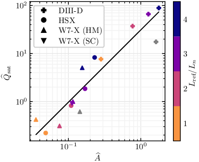
The results of this comparison are plotted in Fig. 1, which exhibits a strong correlation between the turbulent electron energy flux and AE over several orders of magnitude, in a tokamak and several stellarators, for various values of the density gradient, and for one value of the electron temperature gradient, . Here is the length scale of the electron temperature gradient, with being the minor radial coordinate. The density gradient has an analogous definition , with . We note that classical TEMs are thought to be largely absent in W7-X and ion-driven TEMs could instead be the dominant trapped-particle instability Proll et al. 2022; Plunk et al. 2017. These instabilities derive energy from the ions instead of electrons, but we nevertheless include these data points in Fig. 1. A power law is found by fitting a straight line to this doubly logarithmic plot, which gives
| (11) |
This relation can be understood in the following manner. From the definition of the energy flux given in Eq. (10), we crudely estimate this flux as
where the angular brackets denote a volume average. The integral in this expression is bounded by the AE, and we thus set . The square of the drift velocity,
is proportional to the gyrokinetic energy of the electric field. Since the sum total of the thermal and this field energy is conserved Helander 2017, the field energy is also bounded by the AE. Hence we estimate , which gives
| (12) |
in agreement with the observed power law, within error bars.
Conclusions. As we have seen, it is possible to express the AE of trapped electrons in a slender flux tube of elliptical cross section in analytical form, which enables this quantity to be calculated efficiently. Since the AE represents a rigorous upper bound on the energy that can be converted into turbulent fluctuations, it is natural to compare it with the outcome of gyrokinetic simulations. The turbulent energy flux from the latter has thus been compared with the AE computed in flux tubes whose thickness perpendicular to the magnetic field is a fixed number of poloidal gyroradii. For TEM turbulence, one finds a strong correlation over several orders of magnitude and across a range of devices. The energy flux is found to be proportional to AE3/2.
These results are encouraging as they suggest a close connection between turbulent transport and AE, which could be used for quickly assessing confinement properties of magnetic configurations without gyrokinetic simulations. The AE could serve as a proxy function in stellarator optimisation, both for new stellarator designs as well as existing devices, where one may adjust coil currents and plasma profiles to find AE-minimizing configurations. It is however not known whether the close correlation between AE and energy transport persists in plasmas with ion temperature-gradient-driven turbulence. Such turbulence draws energy from the ions, which are not constrained by the invariance of , a fact that needs to be accounted for in the calculation of the AE.
The authors are grateful for the valuable discussions with J. Ball, T. Görler, M.J. Pueschel, and M.J. Gerard. This work was partly supported by a grant from the Simons Foundation (560651, PH), and this publication is part of the project “Shaping turbulence – building a framework for turbulence optimisation of fusion reactors”, with Project No. OCENW.KLEIN.013 of the research program “NWO Open Competition Domain Science” which is financed by the Dutch Research Council (NWO). This work has been carried out within the framework of the EUROfusion Consortium, funded by the European Union via the Euratom Research and Training Program (Grant Agreement No. 101052200 — EUROfusion). Views and opinions expressed are however those of the author(s) only and do not necessarily reflect those of the European Union or the European Commission. Neither the European Union nor the European Commission can be held responsible for them.
References
- Lorenz (1955) E. N. Lorenz, Available potential energy and the maintenance of the general circulation, Tellus 7, 157 (1955).
- Gardner (1963) C. S. Gardner, Bound on the energy available from a plasma, Phys. Fluids 6, 839 (1963).
- Berk et al. (1970) H. L. Berk, C. E. Nielsen, and K. V. Roberts, Phase space hydrodynamics of equivalent nonlinear systems: Experimental and computational observations, Phys. Fluids 13, 980 (1970).
- Bartholomew (1971) P. Bartholomew, On the theory of stability of galaxies, Mon. Not. R. Astron. Soc. 151, 333 (1971).
- Stahl et al. (1998) B. Stahl, A. Schröer, H. J. Ziegler, and H. Wiechen, A quantitative model for relaxation of rotationally invariant collisionless self-gravitating systems, Phys. Scr. 1998, 93 (1998).
- Chavanis (2012) P. H. Chavanis, Dynamical stability of infinite homogeneous self-gravitating systems and plasmas: Application of the Nyquist method, Eur. Phys. J. B 85, 229 (2012).
- Lemou et al. (2012) M. Lemou, F. Méhats, and P. Raphaël, Orbital stability of spherical galactic models, Invent. Math. 187, 145 (2012).
- Baldovin et al. (2016) F. Baldovin, A. Cappellaro, E. Orlandini, and L. Salasnich, Nonequilibrium statistical mechanics in one-dimensional bose gases, J. Stat. Mech. Theory Exp. 2016, 063303 (2016).
- Kolmes and Fisch (2020) E. J. Kolmes and N. J. Fisch, Recovering Gardner restacking with purely diffusive operations, Phys. Rev. E 102, 63209 (2020).
- Helander (2017) P. Helander, Available energy and ground states of collisionless plasmas, J. Plasma Phys. 83 (2017).
- Helander (2020) P. Helander, Available energy of magnetically confined plasmas, J. Plasma Phys. 86 (2020).
- Kadomtsev and Pogutse (1967) B. B. Kadomtsev and O. P. Pogutse, Plasma instability due to particle trapping in a toroidal geometry, Sov. Phys. JETP 24, 1172 (1967).
- Dannert and Jenko (2005) T. Dannert and F. Jenko, Gyrokinetic simulation of collisionless trapped-electron mode turbulence, Phys. Plasmas 12, 072309 (2005).
- D’haeseleer et al. (2012) W. D. D’haeseleer, W. N. G. Hitchon, J. D. Callen, and J. L. Shohet, Flux Coordinates and Magnetic Field Structure: A Guide to a Fundamental Tool of Plasma Theory (Springer Science & Business Media, New York, 2012) pp. 100–107.
- Hall and McNamara (1975) L. S. Hall and B. McNamara, Three-dimensional equilibrium of the anisotropic, finite-pressure guiding-center plasma: Theory of the magnetic plasma, Phys. Fluids 18, 552 (1975).
- Jenko et al. (2000) F. Jenko, W. Dorland, M. Kotschenreuther, and B. N. Rogers, Electron temperature gradient driven turbulence, Phys. Plasmas 7, 1904 (2000).
- Beer et al. (1995) M. A. Beer, S. C. Cowley, and G. W. Hammett, Field aligned coordinates for nonlinear simulations of tokamak turbulence, Phys. Plasmas 2, 2687 (1995).
- Hörmander (2015) L. Hörmander, The Analysis of Linear Partial Differential Operators I: Distribution Theory and Fourier Analysis (Springer, New York, 2015) pp. 136–137.
- Rosenbluth and Sloan (1971) M. Rosenbluth and M. L. Sloan, Finite stabilization of the collisionless trapped particle instability, Phys. Fluids 14, 1725 (1971).
- Helander (2014) P. Helander, Theory of plasma confinement in non-axisymmetric magnetic fields, Rep. Prog. Phys. 77, 087001 (2014).
- Proll et al. (2012) J. H. E. Proll, P. Helander, J. W. Connor, and G. G. Plunk, Resilience of Quasi-Isodynamic Stellarators against Trapped-Particle Instabilities, Phys. Rev. Lett. 108, 245002 (2012).
- Helander and Sigmar (2005) P. Helander and D. J. Sigmar, Collisional Transport in Magnetized Plasmas, Vol. 4 (Cambridge University Press, Cambridge, England, 2005) pp. 127–129.
- Görler (2010) T. Görler, Multiscale effects in plasma microturbulence, Ph.D. thesis, Universität Ulm (2010).
- Proll et al. (2022) J. H. E. Proll, G. G. Plunk, B. J. Faber, T. Görler, P. Helander, I. J. McKinney, M. J. Pueschel, H. M. Smith, and P. Xanthopoulos, Turbulence mitigation in maximum-J stellarators with electron-density gradient, J. Plasma Phys. 88, 905880112 (2022).
- (25) To prevent the electron temperature gradient mode from affecting the TEM turbulence in these simulations, the ratio of the electron over the ion temperature has been increased to , and the smallest and largest resolved binormal wavenumber were chosen to be and (W7-X) / (DIII-D) respectively.
- Plunk et al. (2017) G. G. Plunk, J. W. Connor, and P. Helander, Collisionless microinstabilities in stellarators. Part 4. The ion-driven trapped-electron mode, J. Plasma Phys. 83 (2017).