Tadpole type motion of charged dust in the Lagrange problem with planet Jupiter

Let $w_{T}=w_{T}(X_{j},\vec{X}_{0};\beta;\gamma)$ be the maximum libration amplitude of the $j$-th component $X_{j}=X_{j}(t)$ of vector $\vec{X}=\vec{X}(t)$ during the integration time $0\leq t\leq T$, starting with the initial condition $\vec{X}_{0}=(a_{0},e_{0},i_{0},\Delta\omega_{0},\Omega_{0},\sigma_{0})$, and for fixed values of the parameters $\beta$, $\gamma$. Let $\vec{X}^{*}=(a^{*},e^{*},i^{*},\Delta\omega^{*},\Omega^{*},\sigma^{*})$ be the initial condition that defines the location of $L_{4}$ with $a^{*}=a_{J}$, $e^{*}=e_{J}$, $i^{*}=i_{J}$, $\Delta\omega^{*}=60^{\circ}$, $\Omega^{*}=\Omega_{J}$, and $\sigma^{*}=60^{\circ}$ (or $\Delta\omega^{*}=300^{*}$, $\sigma^{*}=300^{\circ}$ in case of $L_{5}$). For vanishing values of the parameters $\beta$, $\gamma$ and in exact steady-state configuration we have $w_{T}(X_{j},\vec{X}^{*},0,0)\simeq 0$ for all $j$, while for non-zero $\beta$, $\gamma$ we generally find $w_{T}(X_{j},\vec{X}^{*},\beta,\gamma)=\delta_{j}$ with $\delta_{j}>0$ and $j=1,\dots,6$. To obtain a minimum libration amplitude solution we minimize $w_{T}$ with respect to $X_{j}$ starting in the vicinity of $\vec{X}^{*}$, say $\vec{X}_{\varepsilon_{j}}^{*}$ with $X_{j}(0)=X_{j}^{*}\pm\varepsilon_{j}$ and positive $\varepsilon_{j}$:

Let $\vec{X}_{\varepsilon_{j},r}^{*}$ be the initial condition during the $r$-th iteration process with $\vec{X}_{\varepsilon_{j},0}^{*}=\vec{X}_{\varepsilon_{j}}^{*}$. We start with a set of initial conditions on a grid in $(a,\sigma)$ using $a(0)=a_{J}(1-\beta)^{1/3}\pm\varepsilon_{1}$ and $\sigma(0)=\sigma^{*}+\varepsilon_{6}$ with $\varepsilon_{1}>0$ and $0\leq\varepsilon_{6}\leq 120^{\circ}$ and integrate (1) up to time $T$. Here, the choice for $a(0)$ is motivated by the estimate that follows. Kepler’s 3rd law for planet Jupiter takes the form:

while the law for the dust particle, including radiation pressure, becomes:

Eliminating $\mu$ in above equations we find the relation

and taking into account $n_{J}=n$, in presence of a 1:1 MMR, we finally arrive at

Next, we choose, out of the set of orbits, the initial condition with the minimum libration amplitude solution and identify it with $\vec{X}_{\varepsilon_{1,6},r=1}^{*}$ and repeat the above iteration step with smaller $\varepsilon_{1}$, $\varepsilon_{6}$ to obtain $\vec{X}_{\varepsilon_{1,6},r+1}^{*}$. The iteration stops if no significant decrease in libration amplitude can be found anymore when decreasing $\varepsilon_{1}$, $\varepsilon_{6}$. Let $a^{**}$, $\sigma^{**}$ be the initial condition of the minimum libration amplitude solution at the final iteration step $R$. As it turns out the choice $a(0)=a^{**}=a_{J}(1-\beta)^{1/3}$ is the correct choice for the minimum libration amplitude solution for $\gamma=0$ while $\sigma(0)=\sigma^{**}$ is shifted from the equilibrium of the classical problem with increasing value of $\beta$. Next, we repeat above procedure by fixing $a(0)=a^{**}$, $\sigma(0)=\sigma^{**}$, and minimizing $w_{T}$ with respect to $X_{2}(0)=e(0)$, $X_{4}(0)=\Delta\omega(0)$ on a grid $(e,\Delta\omega)$ and using $\varepsilon_{2}$, $\varepsilon_{4}$. We start by integrating (1) with initial conditions $e(0)=e_{J}\pm\varepsilon_{2}$ and $\Delta\omega(0)=\pm 60\pm\varepsilon_{4}$ with $\varepsilon_{2},\varepsilon_{4}>0$, and again identify the initial condition that results in the minimum libration amplitude solution with $\vec{X}_{\varepsilon_{2,4}=0,r=1}$. We repeat the iterative procedure to obtain $e^{**}$ and $\Delta\omega^{**}$ at iteration step $r=R$. As it turns out, for the case $\gamma=0$, $w_{T}$ is minimal for the choice $e(0)=e^{**}=e_{J}$, while $\Delta\omega^{**}$ gets shifted from the equilibria defined for $\beta=0$ with increasing values of $\beta$ like in the case for $\sigma$.

The whole process is done for different values of $\beta$ and for starting values close to $L_{4}$ and also $L_{5}$. Let us denote by $a_{k}$, $e_{k}$, $i_{k}$, $\Delta\omega_{k}$, $\Omega_{k}$, and $\sigma_{k}$ the final optimal values that minimize $w_{T}$, with $k=4$ in the vicinity of $L_{4}$ and $k=5$ close to $L_{5}$ for fixed value of $\beta$.

The results for variables $\sigma_{k}$ and $\Delta\omega_{k}$ are shown in Fig. 5. On the top we report the value of $\sigma$ (by squares) with the minimum of the maximum libration amplitude during the integration time for given values of the parameter $\beta$ in the vicinity of $L_{4}$ (blue) and close to $L_{5}$ (orange). The lines are obtained from a theory based on the circular restricted three-body problem including solar radiation pressure and the Poynting-Robertson effect (1980ApJ...238..337S; 2021A&A...645A..63Z, see, e.g.) and confirm the values obtained by minimizing (5). At the bottom of Fig. 5 we report the results for $\Delta\omega_{k}$ close to $L_{4}$ (blue) and $L_{5}$ (orange), both obtained by minimizing (5). In both figures we clearly see the shift of the minimum libration amplitude solutions in dependency of parameter $\beta$ up to $1.5$ degrees at $\beta=0.1$. The two panels in Fig. 5 also reveal an asymmetry between the Lagrange points $L_{4}$ and $L_{5}$. While the shift in $\sigma$ from $60^{\circ}$ is more prominent for solutions close to $L_{4}$, in comparison to the shift from $-60^{\circ}$ (close to $L_{5}$), the situation is reversed in the shift of $\Delta\omega$. The findings confirm the results, already obtained in Lhotka and Celletti 2015, where the authors use a semi-analytical approach in the framework of the restricted three-body problem (circular, elliptic, and spatial) that is based on averaged equations of motions.

Next, we repeat by minimizing (5) wrt. $a(0)$, $e(0)$, $\Delta\omega(0)$, $\sigma(0)$ for $\gamma>0$, i.e. for dust grain surface potentials equal $5$ and $10$ Volts, in the same way as for the case $\gamma=0$. We find a strong influence of charge on the dynamics as demonstrated by the example shown in Fig. 6. The figure shows the libration amplitudes $\Delta\sigma$ on a grid of initial conditions $\sigma(0)\times\delta a(0)$, with $\delta a=a-a_{1:1}$, for two different values of $\beta$ and $5$ Volts surface charge in the vicinity of $L_{4}$. The location of the minimum libration amplitude solutions in the uncharged case are given by black-dashed lines and we clearly see that in the presence of charge this location (dark-blue) gets shifted towards smaller values in semi-major axis $a$ and larger values in $\sigma$. The effect becomes stronger for larger values of $\beta$ (allowing larger values in $\gamma$ for same surface potential charge): while the deviation in $\delta a$ is smaller and symmetric with respect to the symmetry line $\delta a=0$ it becomes larger and asymmetric in the case $\beta=0.35$. We also notice that with increasing $\beta$ the region of librational motion shrinks. Solar wind, Poynting-Robertson effect as well as the interplanetary magnetic field strongly affect the dynamics. In the following we report the location and parameters for the minimized solution with respect to librational amplitudes, i.e. the location of the darkest blue region in simulations of the type as shown in Fig. 6, in dependency of the system parameters.

We summarize our study for different values of $\beta$ in case of dust grain surface potentials equal $5$ and $10$ Volts in Fig. 7, 8, where the results are given relative to the solution of minimum libration amplitude of the uncharged case. At the top of Fig. 7 we report the shift $\delta a_{4}$ in blue and relative to $a_{4}$ due to $\gamma>0$ for $5$ Volts. With increasing value of $\beta$ we find a negative shift that becomes larger in magnitude and reaching 0.01 AU for $\beta=0.1$. In Fig. 7 we also report the shift $\delta\sigma_{4}$ in orange and relative to $\sigma_{4}$, that again becomes larger with increasing values of $\beta$ (and $\gamma$) reaching several degrees of offset at $\beta=0.1$. The results in $\delta a_{5}$, $\delta\sigma_{5}$ are shown at the bottom of Fig. 7 with comparable values in $\delta a_{5}$ ($\delta\sigma_{5}$) in comparison with $\delta a_{4}$ ($\delta\sigma_{4}$). We notice the presence of spikes close to $\gamma\simeq 0.01$ in both panels that are also present for different surface potential of the dust grains (see, Fig. 8 in case of $10$Volts). We notice that for larger values of the surface potential these spike like structure is shifted towards smaller values in $\beta$ but still remains close to the value $\gamma\simeq 0.01$.

Where does it come from? A series of simulations with various initial conditions and parameters suggests that the spikes are the result of a commensurability between the precession rate $\dot{\Omega}$ of the ascending node longitude and the period in libration of the resonant angle $\sigma$. As demonstrated in Fig. 9 the variations in amplitude of the angle $\sigma$ are greatly enhanced for the case $U=5V$ (in orange), where the fundamental period in $\Omega$ (and $i$) is about the same as for the resonant argument itself. On the contrary, the amplitude variations stay small during the whole integration period in the uncharged case $U=0V$, and for the case $U=10V$. We remark that the period in $\Omega$ is inversely proportional to the parameter $\gamma$, or $\Gamma$ - as it has been shown in Lhotka and GaleΩ 2019. As a result, for $U=10V$, the period of $\Omega$ and $i$ is only half of the value for $U=5V$, as it is confirmed also by the bottom two panels of Fig. 9. Since the libration period of $\sigma$ stays the same for different values of $\beta$, the values of the parameter $\gamma$ which determine the period of $\Omega$ could finally determine the locations of the spike at the same value of $\gamma$, although the corresponding values of $\beta$ are different, since $\beta\propto 1/R$ while $\gamma\propto U/R^{2}$ - see also (3).

The results for minimum libration amplitude solutions concerning the variables $\Delta\omega_{k}$ and $e_{k}$ are reported in Fig. 10. An important effect of charge, that is clearly visible, is the change of $e_{k}$ wrt. to $\beta$ ($\gamma$) that cannot be seen in the uncharged problem, subject to solar wind and the Poynting-Robertson effect alone. While for $\gamma=0$ we have $e_{k}=e_{J}\simeq 0.050$ we get $e_{k}\simeq 0.040$ for $\beta=0.1$ (top of Fig. 10) and a minimum in $e_{k}=0.045$ close to $L_{5}$ (at the bottom of the figure). The shift of $\Delta\omega_{k}$ for $\gamma>0$ also turns out to be more prominent in comparison to the shifts in $\sigma_{k}$. As we can see in Fig. 8 the maximum shift is about $2^{\circ}$ in $\Delta\omega_{4}$ (top) and about $2^{\circ}$ in $\Delta\omega_{5}$ (bottom).

Once the initial conditions for the minimum libration amplitude solutions have been found we are interested in the extend of the librational regime of motions around $L_{4}$ and in the vicinity of $L_{5}$ in dependency of parameters $\beta$ and $\gamma$. To estimate the ‘libration widths’ we start by integrating (1) using the initial conditions from the previous study and increase $a(0)=a^{*}+\delta a$ with $\sigma(0)=\sigma_{k}$ (with $k=4$ close to $L_{4}$ and $k=5$ in case of $L_{5}$) until i) the maximum value of the resonant argument $\sigma(t)$ goes beyond $\sigma_{5}$ (thus $\sigma(t)>\sigma_{5}$) in case of orbits originating from $L_{4}$ or ii) we find $\sigma(t)<\sigma_{4}$ for integrations starting around $L_{5}$. We report the size of the value $\delta a$ at which the crossing of the librational regime takes place in Fig. 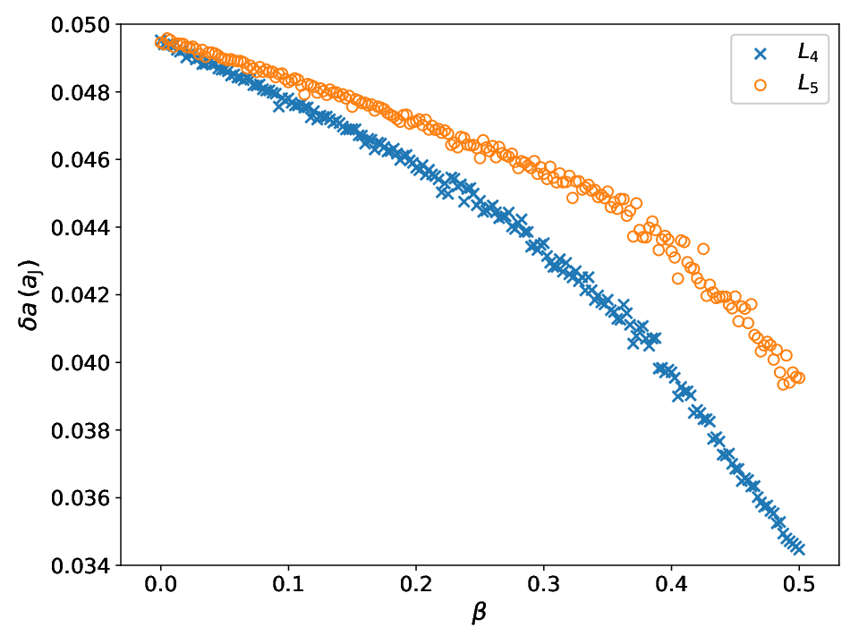11 for different values of the parameter $\beta$ and using $\gamma=0$. We clearly see that due to the additional perturbations $\delta a$ decreases with increasing value of $\beta$ with a steeper slope in case of orbits originating from $L_{4}$ (blue crosses) in comparison to $L_{5}$ (orange circles). Thus, solar wind and Poynting-Robertson effect also triggers the asymmetry between the extend of the two tadpole regimes of motion around $L_{4}$ and $L_{5}$.

The effect of charge on the width of the librational regime of motions is clearly demonstrated in Fig. 6. However, the determination of the maximum libration amplitude is not as straightforward as in the uncharged case. The librational regime (indicated in blue) is tilted and irregular, and moreover depends quite sensitively on the integration time. For this reason we skip the study on the librational regime of motion in the charged problem and investigate the time of temporary capture instead. For this reason, we perform a series of numerical integrations for initial conditions starting at the minimum libration amplitude location close to $L_{4}$ and $L_{5}$ and keep track of the time of temporary capture in the vicinity of the $1:1$ MMR defined by the time at which the dust grain leaves the regime of motion defined by $|a(t)-a^{*}|>0.286$ AU. The choice, that corresponds to about $0.055a_{J}$, is made to cover the full tadpole regime of motions in the pure gravitational case (see top of Fig. 2). The results for the uncharged problem are reported in Fig. 12. Here, the capture time in mean motion resonance with Jupiter starting close to $L_{4}$ is marked by blue crosses, the capture time for orbits starting in the vicinity of $L_{5}$ is shown by orange circles. Interestingly, the capture time, very close to the centers of the CRTBP, is more or less the same for both sets of initial conditions and changing $\beta$.

The results for the case $\gamma>0$, i.e. a dust surface charge potential of $5$ Volts and $10$ Volts is shown in Fig. 13. For small values of $\beta$ capture close to $L_{4}$ and $L_{5}$ takes place on comparable times with a slightly large lifespan for $U=5V$ (crosses) compared to the case $U=10V$. Beyond $\beta\simeq 0.1$ capture times behave more irregular, possibly due to the chaotic nature of the problem. However, we still see an increase in capture time for the smaller value of dust grain surface potential $U$ (compare the location of crosses and circles in Fig. 13).

The shift due to parameter $\beta$ that enters $\vec{F}_{0}$ in (1) has been found to follow $a=a_{J}\left(1-\beta\right)^{1/3}$, the shift in $\sigma$ is given in the upper plot of Fig. 5, obtained numerically, and on the basis of a simplified formula in synodic coordinates (2021A&A...645A..63Z).

To estimate the role of the combined PR and solar wind effect on the Kepler elements we make use of Eq.(14) in Lhotka and Celletti 2015, where the secular effect on semi-major axis $a$ and eccentricity $e$ is simply given by:

References

- Alessi et al. [2019] E.M. Alessi, C. Colombo, and A. Rossi. Phase space description of the dynamics due to the coupled effect of the planetary oblateness and the solar radiation pressure perturbations. Celestial Mechanics and Dynamical Astronomy, 131(9):43, September 2019. doi: 10.1007/s10569-019-9919-z.
- Beauge and Ferraz-Mello [1994] C. Beauge and S. Ferraz-Mello. Capture in exterior mean-motion resonances due to Poynting-Robertson drag. Icarus, 110:239–260, August 1994. doi: 10.1006/icar.1994.1119.
- Beck and Giles [2005] J. G. Beck and P. Giles. Helioseismic Determination of the Solar Rotation Axis. ApJ Letters, 621:L153–L156, March 2005. doi: 10.1086/429224.
- Celletti et al. [2020] A. Celletti, C. Gales, and C. Lhotka. (INVITED) Resonances in the Earth’s space environment. Communications in Nonlinear Science and Numerical Simulations, 84:105185, May 2020. doi: 10.1016/j.cnsns.2020.105185.
- Dvorak and Lhotka [2013] R. Dvorak and C. Lhotka. Celestial Dynamics. John Wiley & Sons, Ltd , 2013.
- Feng and Hou [2019] J. Feng and X. Y. Hou. Secular dynamics around small bodies with solar radiation pressure. Communications in Nonlinear Science and Numerical Simulations, 76:71–91, September 2019. doi: 10.1016/j.cnsns.2019.02.011.
- Fitzpatrick [2012] R. Fitzpatrick. An Introduction to Celestial Mechanics. UK Cambridge University Press, September 2012.
- Grün et al. [1993] E. Grün, H. A. Zook, M. Baguhl, A. Balogh, S. J. Bame, H. Fechtig, R. Forsyth, M. S. Hanner, M. Horanyi, J. Kissel, B. A. Lindblad, D. Linkert, G. Linkert, I. Mann, J. A. M. McDonnell, G. E. Morfill, J. L. Phillips, C. Polanskey, G. Schwehm, N. Siddique, P. Staubach, J. Svestka, and A. Taylor. Discovery of Jovian dust streams and interstellar grains by the Ulysses spacecraft. Nature, 362(6419):428–430, April 1993. doi: 10.1038/362428a0.
- Klačka [2014] J. Klačka. Solar wind dominance over the Poynting-Robertson effect in secular orbital evolution of dust particles. MNRAS, 443:213–229, September 2014. doi: 10.1093/mnras/stu1133.
- Klačka et al. [2012] J. Klačka, J. Petržala, P. Pástor, and L. Kómar. Solar wind and the motion of dust grains. Monthly Notices Royal Astronomical Society, 421(2):943–959, April 2012. doi: 10.1111/j.1365-2966.2012.20321.x.
- Koschny et al. [2019] D. Koschny, R. H. Soja, C. Engrand, G. J. Flynn, J. Lasue, A.-C. Levasseur-Regourd, D. Malaspina, T. Nakamura, A. R. Poppe, V. J. Sterken, and J. M. Trigo-Rodríguez. Interplanetary Dust, Meteoroids, Meteors and Meteorites. Space Science Reviews, 215(4):34, June 2019. doi: 10.1007/s11214-019-0597-7.
- Krüger et al. [2019] H. Krüger, P. Strub, N. Altobelli, V. J. Sterken, R. Srama, and E. Grün. Interstellar dust in the solar system: model versus in situ spacecraft data. A&A, 626:A37, June 2019. doi: 10.1051/0004-6361/201834316.
- Lhotka and Celletti [2015] C. Lhotka and A. Celletti. The effect of Poynting-Robertson drag on the triangular Lagrangian points. Icarus, 250:249–261, April 2015. doi: 10.1016/j.icarus.2014.11.039.