Non-Photorealistic Rendering of Layered Materials: A Multispectral ApproachCCS: Computing methodologies Non-photorealistic renderingCCS: Computing methodologies Computational photographyCCS: Computing methodologies Image processing

Abstract.
We present multispectral rendering techniques for visualizing layered materials found in biological specimens. We are the first to use acquired data from the near-infrared and ultraviolet spectra for non-photorealistic rendering (NPR). Several plant and animal species are more comprehensively understood by multispectral analysis. However, traditional NPR techniques ignore unique information outside the visible spectrum. We introduce algorithms and principles for processing wavelength dependent surface normals and reflectance. Our registration and feature detection methods are used to formulate stylization effects not considered by current NPR methods including: Spectral Band Shading which isolates and emphasizes shape features at specific wavelengths at multiple scales. Experts in our user study demonstrate the effectiveness of our system for applications in the biological sciences.
Keywords:
data acquisition, signal processing, biological illustration, shape from shading, multispectral imaging1. introduction
We address the technical problem of extracting and analyzing shape in layered materials. Our work is inspired by research applications that use multispectral imaging to examine biological materials. It is often important to examine the surface of materials under layers of debris from erosion and other environmental conditions. The biological specimen itself is often composed of composite materials that require multispectral analysis for comprehensive study. For example, ultraviolet fluorescence reveals original color patterns on colorless fossils for species classification (Hendricks 2015) (Figures 1 left and 8). Infrared imaging permits study of subsurface materials hidden under pigments or dyes (Baker et al. 2012) (Figure 1 middle and right). These hidden features provide additional clues about the specimen’s physiological characteristics.
We introduce algorithms that combine multispectral imaging with NPR to communicate these otherwise invisible characteristics of our dataset. Our approach accentuates multispectral information at different material layers in RGBN images (Toler-Franklin et al. 2007) for stylized rendering, biological illustration and scientific study. NPR is effective for scientific illustration (Gooch et al. 1998) because it removes extraneous information (abstraction) while emphasizing relevant details (shape enhancement). Multispectral data has been used to improve detail and color fidelity (Darling et al. 2011) in realistic image synthesis, but has been overlooked in NPR. NPR algorithms still operate on visible-only photos and 3-D geometry. NPR techniques for volumetric data (Joshi 2007; Corcoran et al. 2010) are also limited as they do not formulate stylization rules for signature enhancement across multiple wavelengths. Our goal is to detect and maximize detailed information at different wavelengths. We incorporate contrast enhancement and spectral shape differences to increase fidelity of subtle near-infrared signatures (Albanese and Montes 2011). We also record ultraviolet bispectral shape variations at different magnifications (Tabata et al. 1996) to enhance object scale features. Our contributions include:
- •
Principles and tools for processing multispectral data for NPR including: 2D to 3D alignment that minimizes shape distortion and near-infrared enhancement maps that detect and control shape detail in layered materials. (Section 5).
- •
Multispectral stylization techniques including: spectral band shading that reveals subsurface shape detail, bispectral shading that emphasizes object scale features at different magnifications and multiscale curvature shading and line drawing. (Section 6).
- •
A user study that validates the utility of our approach for applications in biology and related life science research. (Section 7.4).
2. Principles for Multispectral NPR
Pilot Study We began our research by observing eighteen experts (practitioners and researchers) from four disciplines - biology (), anthropology (), forensics () and paleontology () - in their work environments to understand challenges with real-world applications of multispectral analysis in life science research (see supplemental video). We identified three modes of analysis routinely used across these groups: HDR contrast imaging to enhance near-infrared detail while suppressing visible data; the use of fluorescent powders and ultraviolet radiation to reveal latent bio-materials; and micro imaging to examine biological structures. Our experts demonstrated advantages and limitations of these methods for critical research tasks. Inefficiencies included lack of fidelity when working with post processing software (indicating residual pigments with false color (Hendricks 2015) is a well-known example), detail loss at longer wavelengths when denoising images, lack of user control over enhancement parameters and reliance on destructive DNA sequencing methods when micro analysis is ineffective. To address these challenges, we formulated principles and illustrative tools that combine flexible NPR parameter controls with measured multispectral properties, without the complexities (computation, time and expertise) of physically-based rendering solutions. Our principles follow these general processing rules:
- (1)
Apply only minimal filtering to near-infrared data (2-D spectra and normals) to prevent loss of subtle detail.
- (2)
Emphasize subsurface detail in regions where near-infrared contrast is greater than contrast in visible data.
- (3)
Use bispectral reflectance to emphasize structural differences between materials.
- (4)
Incorporate object-scale shape from different magnifications for complex lighting effects.
- (5)
Control stylization effects using measured parameters from real sources for authenticity.
Additional rules are required for analyzing molecular and atomic structures. We focus on non-invasive visualization methods for understanding shape, material composition and anatomical structure.
3. Overview
Figure 2 presents a system overview. We compute the shape of biological materials in the visible, ultraviolet and infrared spectra. Our diverse dataset includes butterfly scales, bone, plants and fossilized materials (cone shells) dating back millions of years. We first demonstrate how current shape from shading approaches fail for our application because they overlook variations in shape that occur at different material layers, and ignore spatially varying reflectance from surfaces with varying material composition. We then explain how we compute normals at different material layers as a function of the emission wavelength of our light source. Our experimental set-up quantitatively validates the accuracy of our normals. Next, we implement 2-D to 3-D alignment across spectral bands, filtering, per-pixel feature detection and near-infrared enhancement. These pre-processes are incorporated into novel NPR stylization methods. The results simulate reflectance properties that occur under different electromagnetic wavelengths which influence behavior, environmental adaptations (Kastberger and Stachl 2003) and species classification. Finally, we conduct a user study with experts in biology and related fields to demonstrate the utility of our approach for life science research.


| GT | Traditional | Takatani13 | proposed | ||||
|---|---|---|---|---|---|---|---|

|
|

|
|

|
|

| |

|

|

|
|
|
|
||
|
|
|
|
|
|
|
| |

|
|
|
|
|
|
||

|

|

|
|
|
|
||
|
|
|
|
|
|
|
| |
|
|
|
|
|
|
|
||
|
|
|
|
|
|
|
||
|
|
|
|
|
|
|
| |
|
|
|
|
|
|
|
||
|
|
|
|
|
|
|
||
4. Multispectral Normal Reconstruction
An object’s appearance depends on material composition and the wavelength of light hitting the surface. Visible light (VIS ) grazing the surface accentuates surface detail. Longer near-infrared wavelengths (NIR ) penetrate top layers revealing subsurface detail. Bispectral reflectance occurs when short ultraviolet wavelengths (NUV ) are absorbed while longer ones are emitted (fluorescence). In this section, we compute normals using a variant of photometric stereo that captures this wavelength-dependent behavior of light.
Photometric stereo (Woodham 1980) assumes a diffuse object, and uses the relationship between observed intensity , the normal and light direction at point (), to compute per pixel normals. Using observations of lit from at least three directions, we solve an overdetermined system of equations to recover .
Traditional photometric stereo will not work for our analysis of layered materials as it primarily recovers the top surface shape, and is prone to artifacts from interreflections in non-diffuse objects (Wu et al. 2011). Multispectral extensions aim to improve quality in top surface normals by combining the most diffuse normals from different spectral wavelengths (Takatani et al. 2013; Sato et al. 2012; Nam et al. 2016), and by removing self-emitted radiance for effective interreflection removal (Nam and Kim 2014). However, these strategies are problematic when longer wavelengths penetrate beneath the surface to reveal underlying geometry that is different. Solutions that merge normal maps, or otherwise combine reflectance data across wavelengths contain inaccuracies from subsurface scattering at surfaces with varying shape at different material layers.
4.1. Approach
Our goal is a practical, computationally inexpensive method to extract shape from at least one subsurface layer with only slight modifications to a standard multispectral photometric stereo set-up. First, we record the observed radiance at each wavelength for light orientations for three exposure values . Unlike other methods, we treat as a separate shape layer, and use information from multiple exposure observations, to limit optimizations to a single spectral band. We detect highlights at intensity peaks that spread outward from to (Figure 4). We examine in the frequency domain as spatial analysis of highlights is challenging with monotone images. We use Welch’s averaged, modified periodogram (Welch 1967) to locate frequencies where the magnitude squared coherence () between and (likewise and ), is lower than the percentile, (divergence for intensity shifts is expected). For two signals, is a function of their power spectral densities and cross power spectral density. Values range from to perfect coherence at . Specular-free images (SF) for highlight detection (Tan and Ikeuchi 2005) have been generated from scene priors without specularities (flash and no flash images) or by substituting color components. Without loss of geometric structure, we compute , the SF image as the difference in pixel intensities with , a highlight-free image at the same tilt angle. Logarithmic differentiation applied to and extracts pure diffuse reflection. Specular highlights are reduced in , by iteratively shifting maximum pixel brightness to that of a more diffuse neighboring pixel. Typical exposure times in seconds are blue and green - , , , red - , , , and - , , , with typically . Additional preprocessing time, image size constraints for FFT, and shadow interference are limitations. Additional exposures are discarded, and per layer normals are computed as:
| (1) |
where is the spectral sensitivity of the camera, is the spectral reflectance of a point, and are the spectrum of the light.
Our capture system includes a radiometric CCD imager with an internal motorized filter wheel (Kim and Rushmeier 2011) for aligned multispectral imaging, essential for accurate per pixel comparison across wavelengths. We also work with affordable visible, and IR modified DSLR cameras (prevalent in our application space). The IR camera is optimized to focus at . External lens filters permit imaging at and , but require a manual focus shift, and vignette compensation. To capture macro detail on small and large samples, we use two light sizes, based on effective attenuation angle and the number of LEDs. Figure 3 summarizes our filters, lights and sensors. See additional information in supplemental materials. Micro imaging is discussed later in this section.
4.2. Validation
Experimental Setup: We quantitatively evaluate the accuracy of our normals in Figure 5. Using our CCD imager, we compute photometric stereo at r, g, b, near-infrared (), and rgb combined () channels on spheres with etched grooves under paint layers. We compare our normals ( and ) with ground truth geometry; 3-D scans of the grooves () and paint layer (). Our spheres, labeled by color, include , a near diffuse inch diameter polytetrafluoroethylene (PTFE), and two one-inch polyoxymethylene (acetal) spheres, and that exhibit specular reflectance. Opacity, thickness, absorption, transmission, and light wavelength (Burleigh et al. 2016) effect optical properties of paint. We chose tempera paint for its opacity and natural composition, like our data. Several paint layers ensure grooves are not discernable in visible light. We do not use synthetic datasets in our analysis because we require a near-infrared source, but include a spectralon sphere as a base-line standard.
Experimental results show that we accurately recover shape beneath the paint layer. We compare with , and with , and use heat maps to visualize the error as angular differences. The numbers show average error. Heat maps , , ,
confirm that we recover all four sets of grooves, and the overall spherical geometry accurately (dark blue, zoom to see details). Average error is lower in and because the diffuse surface has less interreflection artifacts than the reflective acetal examples. Most of our error is due to interreflections in unpainted regions of acetal spheres. Although matrix ranking (Takatani et al. 2013) consistently selected the most diffuse spectra per segment, it did not accurately recover shape in or for or because it combined shape across different material layers (reddish yellow regions). This method had nearly the same performance as our approach (error and respectively) for because, due to the simplicity of our data, the normal map had primarily near-infrared normals. Grooves appear in both normal layers for which transmits red () and infrared (). Conversely, absorbed and , appearing black in our red, blue and filters, and dark grey under the green. In this case, imaging required a high-powered IR light ( to ) and a filter. We did not see grooves below (though one was recorded in the green, lowering expected error in ). We used a full-spectra light and a filter with which had lower reflectance than acetal. Traditional photometric stereo had higher average errors from interreflection and subsurface scattering (, , for and respectively), but low error for () and spectralon ().
Limitations Our method is effective for naturally occurring materials that exhibit near-infrared transmittance. Synthetic polymer-based paint with complex structure and high reflectance hide lower level shape (see supplemental examples). Although we investigate separate channels in the visible range, we use for our rendering, and handle as a separate layer.
4.3. Object-Scale Shape
Thus far, we have focused on visible and near-infrared normals. Bispectral normals from emissive rather than reflective wavelengths approximate shape better when there are specularities ( (Sato et al. 2012; Treibitz et al. 2012)). Bispectral shape recovery is challenging for purely fluorescent (Glassner 1995) objects with changing material composition (Figure 8). Even objects with relatively constant emission spectra are difficult when material concentration varies (Sauer et al. 2011; Zhang and Sato 2011). Hybrid deep learning approaches combine near and far approximation lights to capture spatially varying reflectance (Santo et al. 2020), but ignore effects of light penetration depth. Large volumes of data are required, and simple visible-only datasets are limiting. GPU memory constraints and patch-based operations reduce output quality. Layered material simulations focus on photo realism (Yamaguchi et al. 2019).
We incorporate bispectral shape and luminance in our shading algorithms to enhance object-scale features and structural differences between materials. Combinations of thin translucent and colorful opaque layers in butterfly wings (Tabata et al. 1996) cause hue to vary with light orientation but remain consistent with changes in tilt angle (Figure 9 bottom row). We approximate the emittance spectra from observed bispectral reflectance in micro-images, using a standard Olympus micro camera, common to museums and life science research labs. We image light orientations, limited by the closeness objectives (, and ) to the object. We then compute normals using the visible emission spectra (r, g and b) from ultraviolet excitation (), , which we combine with , only at fluorescing pixels. Though bispectral shape recovery for composite materials is beyond scope, the results () capture more structural detail than current NPR approaches. We now discuss our datasets and layered normals in the context of our guiding principles.

 |
 |
 |
 |
 |
 |
Principle 1 recommends minimal smoothing to preserve longer wavelengths that penetrate deeper, and shorter wavelengths that encode shape details and discontinuities. Figure 6 (middle and right) shows recovered shape at different segment layers for a shell fossil after smoothing.
Principle 2 emphasizes differences in shape which we recover at multiple wavelengths. Figure 6 left shows the shape differences between layers for the normals shown to the right, which we incorporate in our contrast enhancement techniques. In Figure 7, reflectance from the red pigment produces shape in the visible normal map while the near-infrared map captures curvature features


of the underlying bone. Note how the red letter P fades as the near-infrared wavelength increases from to .
Principle 3 leverages bispectral imaging (Sato et al. 2012) to record fluorescence and residual color patterns (Figure 8 top). We use observed fluorescence as emitted red, green and blue intensities under ultraviolet excitation.
Principle 4 incorporates shape variations at different magnifications which are known to influence object-scale reflectance (Figure 9 bottom left). Butterfly wings are complex layered structures with ridges, lamellae and a lattice of microribs (Figure 9 top) that produce complex reflectance properties. Figure 9 bottom right shows how chrominance changes with orientation but not tilt angle. Reflected UV imaging in Figure 10 shows how the structure and composition of a cabbage white butterfly wing influences the absorption and emission spectra.
5. Multispectral Data Processing
5.1. Filtering
Joint bilateral filtering removes residual capture artifacts. When contrast modulation operators are applied to near-infrared intensity values, they often produce values that range close to zero. Following Principle 1, we apply minimal filtering to prevent loss of this information (typically passes using a pixel width filter with domain, range and normal kernel widths of , , and respectively).

5.2. Multispectral Multimodal Registration
Multispectral, multimodal registration is required for sub-pixel accuracy when comparing information across spectral bands from different devices. We modify a Robust Selective Normalized Cross Correlation (RSNCC) (Shen et al. 2014) algorithm (Appendix A). The inputs are visible and near-infrared intensity/normal map pairs. We first generate a composite image at each wavelength using the percentile intensity at each pixel across the multilight stack (from normal computation) to remove shadows that skew results. We use RSNCC to register each to a reference visible image . Dense pixel correspondences are used to generate a global and local alignment transformation between each and .
Next, normals from different spectra must be aligned. RSNCC cannot be applied to normals without introducing shape distortions as it computes similarities between image-based color and gradient features. The three regularization terms in the cost function (Equation 27) use convolution operations that over-smooth normal vectors. Large variations in normals across spectral bands make them unsuitable as a similarity measure. We iteratively transform color and geometry without disassociating per-pixel normals from corresponding pixels in the intensity map. We use the homography matrix from the global alignment of with to perform a coarse rigid body alignment that shifts the pixel coordinate location of each normal in the image frame. We do not use the RSNCC cubic bilinear interpolation to shift and blend pixel values but shift normal positions directly. Assuming one camera is fixed, we use the homography relationship between the two images (Figure 11)to transform the position to . is not ideal when computed on small regions or a broad range of focal lengths. Thus, we use an affine homography transformation by modifying the last row of to . Finally, we apply the transformation from the localization phase. We adjust the process by filtering on to prevent foreshortening effects and limit discontinuities from data loss which occur when pixel positions are shifted (Toler-Franklin et al. 2007). The cost functions we choose are more effective (than SIFT and mutual information) because they are resistant to noise, intensity variations, gradient reversal and structural inconsistencies between near-infrared and visible images. Figure 11right plots the error between ground truth near-infrared normals from aligned imaging with our CCD (with motorized filter wheel) an infrared DSLR camera aligned using global and local transformations from traditional RSNCC and our modified RSNCC. The reference stores the combined r, g, b CCD images. Modified RSNCC (solid line) is more accurate than traditional RSNCC (dotted line) for different specimens captured with different intrinsic and extrinsic camera parameters.
5.3. Near-Infrared Shape Analysis
We introduce two shape analysis methods, a dynamic light dependent approach and a static light independent approach, that identify where to incorporate near-infrared features in stylization. Building upon Principle 2, both algorithms operate on visible and near-infrared normals, and , to generate near-infrared enhancement maps, , per-pixel weights that quantify the amount of contribution from each spectral wavelength.
Dynamic Near-Infrared Enhancement uses contrast modulation operators from signal processing to compare wavelength dependent shape functions. We compute dynamically by comparing the local contrast in Lambertian shape computed on and :
| (2) |
where is a luminance function that depends on wavelength and surface normal orientation. Lambertian map stores where is the normal at pixel in and is the light direction. We choose interactively using grazing angles until features appear clearly. This is analogous to the raking light used to exaggerate local details in art analysis. We compute another Lambertian map using and the same . Finally, a Michelson contrast modulation operator, , is applied to each Lambertian map:
| (3) |
where is the Lambertian map at wavelength and and are the minimum and maximum luminance over a pixel neighborhood . The operator identifies variations in shape by measuring the relationship between the spread and the sum of and over localized regions in . Small values produce sharper contrast while larger values produce smooth variations. The results are two per-pixel contrast maps and . Equation 4 computes the contrast difference between and at pixel to encode shape differences in and :
| (4) |
| (5) |
We clamp below a threshold () to zero as relative spectral shape differences are negligible. Using thresholded differences, , the value stored at the pixel in the final enhancement map is a weight on the interval that satisfies Equation 5. Luminance varies with wavelength. Thus, lighter pixel values indicate changes in shape relative to the average at each spectra.

 |
 |
 |
 |
 |
 |
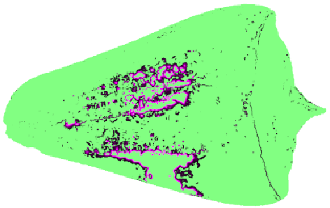
We chose Michelson contrast because it detects multiscale features in both bright and dark regions by examining differences in maximum and minimum intensity within a region rather than differences in foreground and background intensity (Weber contrast) or standard deviation from mean intensity (RMS). Lambertian shape in (Figure 12 b) reveals structures not apparent in (Figure 12a). Close-ups (Figure 12 d-f and g-i) compare details at each spectra with corresponding enhancement maps (shown left to right). Regions for enhancement (magenta) are brighter for higher contribution weights. Only regions where shape in does not appear in are captured because we identify enhancement where is greater than . Other formulations transfer unwanted visible shape to . Using to position is also key (Figure 13).
Static Near-Infrared Enhancement leverages relationships from differential geometry to compute the full near-infrared feature set. A linear shape operator is applied at each wavelength to compare local curvature using derivatives of surface normals in and with respect to direction . Operator is a Weingarten Map:
| (6) |
where , , and are coefficients of the first fundamental form and , and are coefficients of the second fundamental form
and is defined at each tangent plane . We extract algebraic invariants of and (Ohtake et al. 2004) including normal curvature, principle curvatures and mean curvature (, and , and respectively). After smoothing with foreshortening correction (scales normals by ), a Sobel operator is applied to and to approximate and and compute curvature maps and . Per pixel curvature differences determine regions for near-infrared enhancement:
| (7) |
| (8) |
| (9) |
The thresholded difference at pixel , (), is used to compute the enhancement value (Equations 8 and 9). Normalization is applied to generate the final contribution weights. Weighting different shape types has negligible effect. We only emphasize regions where near-infrared curvature is greater (beyond a threshold) regardless of orientation as regions of similar curvature already appear in visible renderings. Thus, when comparing concave and convex shapes, near-infrared shape is accentuated if one curves more than the other, and any intrinsic function of and may be used despite differing signs (directions). Normal curvature produces more consistent results than methods like mean curvature, which loses detail after normalization.
 |
 |
 |
| scrimshaw ship | ||
 |
 |
 |
| scrimshaw tree |
|
|
 |
 |
|
 | |
|
|
 |
 |
|
 | |
|
|
 |
 |
|
 | |
| Dynamic | Dynamic | Static |
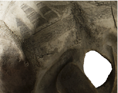
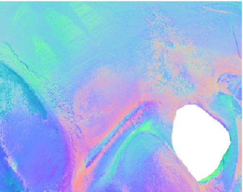
Static enhancement eliminates false enhancement readings from dynamic lights that illuminate regions in either or . Static enhancement reveals all features (both circular features appear in Figure 15 bottom right) while dynamic enhancement reveals different features at different light orientations (good for feature selection, Figure 15 bottom left and middle). Static enhancement produces continuous, smoothly varying differences suitable for shading while dynamic enhancement emphasizes discrete shapes.
6. Multispectral Stylization
Building upon principles and tools introduced in Sections 2 and 5, we present multispectral NPR stylization techniques that express the shape, composition and structure of biological materials.
6.1. Spectral Band Shading
Spectral band shading emphasizes multiscale near-infrared shape across multiple wavelengths for each surface orientation. The spectral band control enabled by the integration of near-infrared enhancement maps (Section 5) distinguishes Spectral Band Shading from other multiscale NPR enhancement algorithms (Fattal et al. 2007; Toler-Franklin et al. 2007; Rusinkiewicz et al. 2006). We develop strategies for simulating narrow and broad band transmission filters that suppress visible content while accentuating near-infrared wavelengths. Our methods combine spectral wavelengths (horizontally) at each scale before combining (vertically) across frequencies.
We start with two stacks of smoothed normals in the visible and near-infrared ( and ) and near-infrared enhancement maps computed at each smoothing level . The shading contribution at pixel on from each spectra is:
| (10) |
| (11) |
| (12) |
We use weight to combine spectral contributions before applying a shape enhancement term (typically 35). For the remainder of the paper, we refer to near-infrared enhancement maps in equations as and distinguish dynamic from static in the main body of the text. In spectral band shading, can be dynamic or static depending on the light direction choice . We discuss application specific options for later in this section. For now, assume is used to generate with dynamic lighting at each level.
 |
 |
 |

| Combined | Dynamic Focus | Combined | Dynamic Multilight | Combined | Static Principle | ||
|---|---|---|---|---|---|---|---|
 |
 |
 |
 |
|
 |
|
|
Next, we incorporate multiple wavelengths using two methods. The first is analogous to a narrow bandpass filter where a specific wavelength dominates (Figure 20 b). For each pixel, we compute a per-wavelength contrast modulation and choose the near-infrared wavelength at the current pixel, to be the spectra with the highest modulation value. We use this value to compute the contrast at this pixel. Thus, contrast differences shift between wavelengths from pixel to pixel as each wavelength competes for its contribution. When is dynamic, the weight is:
| (13) |
where:
| (14) |
When is static, weights are computed using the wavelength with the maximum curvature value in :
| (15) |
where:
| (16) |
The second method combines shape contributions from different near-infrared wavelengths at each level linearly so that they perform like a broad band filter (Figure 20 a). We compute and for each wavelength. We then normalize the per-pixel contributions in each by the number of wavelengths. We compute Equation 12 for each wavelength. For both approaches, the final pixel shading is combined vertically across the smoothed stack weighted by , the normalized kernel widths:
| (17) |
We shade with soft toon clamped from . Smoothing consists of a base layer lit by a global light in the upper left for flat objects (lower for curved objects). The pixel width of our smoothing window increases by powers of two. A geometric series is used to increase the width of our Gaussian kernels and (which are consistent across spectral bands at each level). A base layer plus five levels of smoothing are sufficient for our datasets. Results are shown in Figure 17. We set , , and to .
Following Principle 5, we use measured parameters for stylization controls that illustrate the power of our algorithm.
Shape:
The analysis in Section 5 provides the foundation for our shape enhancement effects. Smoothing and sharpening near-infrared detail is achieved by widening and narrowing , the contrast modulation window from Equation 3 (Figure 16). Figure 17 shows how the frequency term controls sharpness by pushing near-infrared enhancement up and down the normal stack. Selective enhancement at any number of wavelengths exploits robust shape features that persist at longer wavelengths that are less prone to noise. Recall that details from (which are pre filtered for noise removal) will smooth away while significant information remains in . Using a weighting term when combining visible and near-infrared information also eliminates undesirable artifacts and blends the two spectra with more gradual transitions for a smooth shading result.
Lights:
The options for for dynamic spectral band shading are shown in Figure 19 a, b and c. Enhancement map lights emphasize near-infrared detail where there are greater shape variations in as both and are positioned at , the light used to generate at each level. The multilight option maximizes shape from both spectra by setting and to a light projected into the tangent plane of the next smoothed normal in and respectively. The system generates the single focus light to maximize contrast in a user chosen focus region by positioning to maximize the near-infrared contrast in for persistent features across the normal stack. The static principal light uses pre-computed per-pixel curvature values to place along per-pixel principal directions in each spectral band at each level. This accentuates near-infrared detail where the subsurface layer has sharply varying curvature. Figure 18 shows how three light options effectively combine multispectral shape information at smoothing level .
Color:
Layered rendering effects are inspired by our pilot study, where we observed multispectral HDR contrast enhancement that suppressed visible content while enhancing subtle near infrared detail in crime scene photos. In Figure 20, we visualize signatures at specific wavelengths. A multispectral blending function shifts between visible color to near-infrared intensity across wavelengths by adjusting a near-infrared blend function from . This intensity map is used in spectral band shading to create a background reference image. Next, each wavelength is associated with a color from a user specified palette and rendered on top of the reference. Weights (Equations 13 and 15) control the visual contribution of each wavelength in the foreground.
 |
 |
 |
 |
| (a) | (b) | (c) | (d) |

6.2. Multispectral Curvature and Line Drawing
We combine spectral band shading with multiscale multispectral curvature shading (Toler-Franklin et al. 2007) to simulate per pixel lighting. The algorithm substitutes the diffuse component with curvature values (Section 5.3) computed on and . The wide range of curvature values in our specimens make it difficult to see subtle details as high curvature regions are pushed to white while small curvature regions are gray. Near-infrared curvature values are more readily apparent than visible ones. To mitigate this, we scale curvature values by a user defined parameter . We double when working with visible spectra. The scaled curvature values are then combined across spectra using enhancement maps. We clamp the shaded output between to darken valleys and to brighten ridges. The contribution at each level is a function of , the width of the domain filter. We also extract shape conveying lines directly from multispectral normals. Suggestive contours occur as a contour is forming on the horizon (DeCarlo et al. 2003). We create a head-lit image , search for minima of intensity over a local neighborhood and extract lines where a majority of pixels are darker than the current pixel. Discontinuity lines are computed by searching for locations where neighboring normal orientations are very different and normals are not perpendicular to the view. We also find locations of maximum normal curvature in the principal directions (Section 5). Smoothing and denoising are key for creating aesthetically pleasing results as the variation of parameters for robust line extraction changes across spectra. Figure 21 shows curvature shading and multispectral line extraction. The mean filter radius, pixel neighborhood and threshold for suggestive contours are , and . View and normal thresholds for discontinuity lines are and .

6.3. Bispectral Shading
We present multiscale shading variants to enhance object-scale anatomical features in layered materials by incorporating bispectral shape, bispectral luminance, and multiple diffuse reflectance maps.
Bispectral shape:
In Figure 22 b, multiscale bilateral filtering on combined visible and bispectral normals (, Section 4) enhances the shape of guard cells so that they are easily identified in micro-images. Guard cells (Figure 22a) are two specialized curved cells that surround stomata, tiny openings found in the lower epidermis of a leaf underneath a thin cuticle layer. Manual imaging methods use static photographs of peal leaf-imprints in a process which may damage the specimen. Our non-destructive alternative controls levels of detail in observations of the surface. Shape map (Figure 22c) shows more details of the guard cell structure (like the opening), than shape map (Figure 22d) due to object-scale detail in . Shadows and yellowish color map tones are added for curvature enhancement.


Bispectral Luminance:
Our multilight enhancement is unique because it captures features that are only revealed by the interaction of short ultraviolet wavelengths with nanoscale structures (Figure 10). Multilight enhancement methods (Fattal et al. 2007) (MLIC) separate luminance and chrominance, operating in space. Details () from multiscale luminance () image decomposition are combined before adding chrominance ( and ):
| (18) |
Base image, , combines shading across all input at the coarsest scale. User parameter () controls interpolation.
We introduce a new structural term computed from bilateral filter decomposition of bisectral reflectance maps captured from all light directions and scales . We control the sharpness (apparent focus) of shape details, by replacing the visible decomposition term, , with at pixels in the bispectral luminance map, where the intensity is greater than a threshold . These pixels are emitting visible light from uv excitation (). We compute from difference images of smoothed luminance for each :
| (19) |
where:
| (20) |
and is a normalized sum of all detail weights. Weight, is a per wavelength gradient with high frequency noise removed. The detail function computes the difference in luminance between levels across all lights and scales. As discussed, is for , otherwise . Each pixel in is selected directly from or at the course most level (without detail enhancement).
| (21) |
Unlike prior methods, we compute a linear combination (and ) sampled from more than one reflection map, which we combine with before converting to RGB color space. Our bispectral formulation eliminates shadows (a limitation of traditional methods) across all MLICs in regions with high structural detail (apparent in fluorescence). Light dependent chroma effects are simulated by incorporating multiple visible diffuse reflection maps when shading (see Multiple Diffuse Maps for further reasoning behind this step):
| (22) |
| (23) |
| (24) |
Figure 23 compares our method for three light orientations (three right columns) with traditional MLIC enhancement (left column). Increasing from to creates an effect like focusing a camera lens. The out-of-focus threshold is approached in Figure 23 d and h. The combined effect of and increases apparent depth of the cell in Figure 23 c and g compared to flatter renderings in Figure 23 a and e. Biologists manually count guard cells to determine the number of sets of chromosome pairings in plants ( (Mishra 1997)), an evaluation method in our user study.

Multiple Diffuse Maps:
We compute weights where is an angular difference between the input light direction and for each associated diffuse reflectance map, and generate a per-pixel color by interpolating between diffuse reflectance maps. These are not precise approximations for iridescence (Figure 9), but demonstrate effects not available in traditional NPR. Compare the 3-D-like quality of the scale in Figure 24 (b-d) with the traditional approach Figure 24 (a) that uses constant chroma and visible-only structure. Figure 25 shows hue variation at different magnifications.

7. User Study
We conducted a user study to validate that our multispectral analysis methods: (1) cannot be achieved with current NPR techniques, (2) improves precision in real-world life science research tasks and (3) have effective parameter controls. We access how material properties in authentic multispectral data, including layered shape, enable new forms of analysis beyond the aesthetic-based capabilities of current NPR. We formulate quantitative metrics to measure user accuracy performing the same research task with traditional NPR and our algorithms in a between subjects user study. We also report qualitative feedback on user experience using parameter controls.
7.1. Participants and Methodology
We recruited participants. Among these, were self-categorized as experts in one of four disciplines: biology (), anthropology (), forensic science () and paleontology (). Eighteen () self-categorized as novices with background knowledge in these fields, but less practical experience. Participants in the pilot study did not participate in the user study. Participants did not receive compensation.
We designed two research tasks based on pilot study findings - Feature Selection and Guard Cell Counting. No training was required. Tasks were completed remotely over a web-based interface to our client-server implementation. Simple instructions were presented as four general steps: examine the specimen (which was rendered in either a traditional or multispectral style), locate specific features, adjust pan-zoom and slider controls for feature enhancement, select the features in the rendered image or choose not found.
Quantitative metrics were used to evaluate selection accuracy. Selections were categorized as correct if the selection circle intersected feature pixels ( accuracy) or occurred within an allowable distance d from the feature (with accuracy decreasing exponentially with distance). Incorrect selections occurred outside d or when the not found button was selected. We use a pixel selection radius with pixels for a resolution image. Users also provided qualitative feedback by rating the effectiveness of parameter controls on a scale of . Participants were not given time constraints but took on average - minutes per task. Most participants () participated in only one task and participated in both. We now describe our research tasks.
Feature Selection
is used to identify biological structures in specimens. Participants were instructed to find shape features in a rendered image. Features were visualized separately as enhancement map icons. Three datasets were used. Each dataset was assigned four features - half visible and half near-infrared. The participants were randomly assigned spectral band shading or a traditional NPR algorithm. Traditional NPR included Toon, Gooch and Exaggerated shading, and multi-pass joint bilateral filtering combined with Lambertian shading. Assignments were distributed evenly among experts and novices such that half ( experts, novices) received spectral band shading and half (8 experts, 8 novices) received traditional NPR shading ( experts and novices for each traditional algorithm). User accuracy per algorithm was evaluated.
Guard Cell Counting
is used to identify organisms with more than two paired (homologous) sets of chromosomes. The number of chromosome sets in somatic cells (ploidy level) is directly tied to stoma size (area covered) and stomatal density (number of stomata per unit sq area of a leaf). These values differ from species to species( (Mishra 1997)). As chromosome sets increase, stomata size increases and density decreases. Participants were instructed to locate and select guard cells by placing and resizing a marker to completely cover the cell in micro-image ( objective) visualizations. An example guard cell was displayed separately as a reference. There were participants, randomly assigned to one of three visualization types: visible photo, traditional MLIC, our bispectral MLIC shading, Lambertian shading with bilateral filtering on our and traditional Lambertian shading with bilateral filtering on . Images were evenly distributed among experts and novices ( novices and experts per image type). Counts were used to determine stoma size and stomatal density, and ultimately the number of sets of chromosome pairs and results were compared with published results ( (Nesom 1983)) from manual methods (Figure 22a). We also consulted experts from our pilot study for confirmation.
7.2. Evaluation Metrics


Feature selection results show our NPRplus multispectral analysis system permits scientific analysis not possible with current NPR. We computed the average error (, Section 7.1) over all near-infrared features for each algorithm. Both experts and novices detected near-infrared sub-surface features at a lower error rate than traditional methods. Figure 26 top shows expert error (spectral band , exaggerated , Gooch , Toon , Bilateral ). Novice error is shown on the bottom (spectral band , exaggerated , Gooch , Toon , Bilateral ). A similar trend occurred when considering both visible and near-infrared features. Figure 27 top shows expert error (spectral band , exaggerated , Gooch , Toon , Bilateral ). Novice error is shown on bottom (spectral band , exaggerated , Gooch , Toon , Bilateral ).


Our algorithms improve precision in real research tasks. Figure 28 shows a feature ranking exercise. The axis plots precision (accuracy) of correct selections ordered from high to low. The axis plots the fraction of correct selections over the total correct features listed. Incorrect selections were excluded. Participants using spectral band shading were more accurate for a longer recall. Participants who worked primarily with digital media - images and software - were more accurate than those who worked with traditional mediums - printed photographs and x-rays on light tables. Figure 29 left compares expert (media , traditional ) and novice (media , traditional ) accuracy based on modes of work. All novices using spectral band shading had digital media experience, while our expert pool was split traditional and digital (Figure 29 right). This explains why novices outperformed experts when using spectral band shading.


Figure 30 shows that dataset characteristics influence the selection error. Exaggerated shading, the most effective classic method had a higher error rate for the painted bone than it did for the monotone shell as participants could not find features underneath the red paint. Gooch shading had high error rates throughout. Overall, our methods were more effective for feature selection when compared to traditional methods combined across all features (Figure 31). Experts were more effective, and novices were more effective.
Guard Cell Counting with enhanced bispectral detail was more precise than traditional NPR or manual methods. We correctly predicted the number of sets of chromosome pairs in our specimen ( (Nesom 1983)) as diploid (two). Stoma counts were recorded as the number of markers. Marker heights and widths were converted to microns before computing stoma area and stomatal density. Table 1 records the number of correctly identified stoma, and error between computed stomatal density and published results. Novice performance varied greatly. Some selected only a couple of guard cells with high precision producing low SD error (MLIC: and Bilateralplus: ), while others selected many, with moderate correct selections but good precision, resulting in low overall recalls (highest: for MLIC). Multispectral information was effective as novices had the lowest RMSE and MAPE error for bilateral filtering methods (, respectively for bilateralplus and , respectively for MLICplus). Experts performed consistently, with a higher recall () for bispectral shading than visible photographs (). RMSE and MAPE for the photograph ( respectively) decreased for the rendered visualizations with the lowest error for bispectral shading ( respectively). Interestingly, MAPE consistently decreased from for a photograph to for the best case with bilateral shading. We anticipate use of fluorescent properties of the stoma for automatic stoma detection for predicting chromosome pairings.
| Novices | ||||
|---|---|---|---|---|
| Algorithm | Recall | Error metric | ||
| SD | RMSE | MAPE | ||
| Visible photograph | 0.18 | 590.40 | 734.32 | 1.21 |
| MLIC | 0.19 | 22.31 | 351.60 | 0.73 |
| Bilateral | 0.05 | 112.90 | 282.09 | 0.54 |
| Bilateralplus | 0.03 | 66.95 | 220.85 | 0.44 |
| MLICplus | 0.10 | 220.71 | 233.43 | 0.38 |
| Experts | ||||
|---|---|---|---|---|
| Algorithm | Recall | Error metric | ||
| SD | RMSE | MAPE | ||
| Visible photograph | 0.34 | 414.86 | 499.25 | 0.87 |
| MLIC | 0.26 | 200.73 | 384.74 | 0.78 |
| Bilateral | 0.16 | 299.43 | 341.16 | 0.64 |
| Bilateralplus | 0.19 | 188.13 | 199.37 | 0.35 |
| MLICplus | 0.37 | 130.24 | 156.82 | 0.28 |
7.3. Study Limitations
Experts did not have a strong preference for our parameter controls compared to traditional ones, while novices clearly gave higher ratings to our controls (Figure 31 right). This divergence is likely due to the meticulous way experts verified selections, coupled with the broader flexibility in our parameter set requiring a higher learning curve. In guard cell counting, the narrow field of focus and image quality could be improved with HDR imaging, and merging multiple images at different depths of focus.
 |
 |
 |
 |
 |
 |
 |
 |
 |
 |
7.4. Applications
Study results show our pipeline is generalizable to disciplines like biology, forensics and paleontology where visualizing micro structures, sub-surface detail and latent imprints (residual color, bitemarks, fingerprints) are important. Moreover, our system makes complex analysis accessible in simple formats for a broader life science research community. Multispectral datasets provide new information for NPR (Figure 32). Figure 33 illustrates multiscale, multispectral curvature shading and line extraction for analyzing engraved bone carvings (scrimshaw). Spectral band shading with curvature shading emphasizes shapes (grooves and hill features) and suppressed markings. Figure 34 demonstrates spectral band control for studying pigments that change appearance at different wavelengths. Figure 35 shows pipeline flexibility. Near-infrared blending enhances circular patterns on the underside of the butterfly wing. The artistic effect was created by filtering visible color and near-infrared spectra and applying Lambertian shading. Per pixel, per channel blending of quantized near-infrared 2-D spectra creates a toon-like effect.
 |
 |
 |
 |
 |
 |
 |
 |

Related Work We leverage acquisition systems from prior work that use narrow-band pass filters (Habel et al. 2012; Toque et al. 2009; Hordley et al. 2004) to record material properties and incorporate multispectral shape (Brusco et al. 2006; Kim et al. 2012). Our acquired data can be classified with multichannel image data types that store both color and surface shape (Malzbender et al. 2001) in the form of normals (Rushmeier and Bernardini 1999) computed from multi-illumination photography. These data types permit interactive relighting for detail enhancement and have been used to analyze cultural heritage artifacts (Mudge et al. 2010). Our focus is processing and rendering that maximizes the captured data by combining stylization information across spectra, a methodology not available even for volumetric rendering in NPR (Rusinkiewicz et al. 2006; Schein and Elber 2004; Burns et al. 2005).
Our shading methods relate to multiscale NPR decomposition that combines shape details across multilight images (Fattal et al. 2007). Exaggerated shading uses normal stacks to maximize contrast across all frequencies and orientations (Rusinkiewicz et al. 2006). Multiscale curvature shading uses derivatives of surface normals to darken indentations and lighten ridges (Kindlmann et al. 2003; Miller 1994; Zhukov et al. 1998; Toler-Franklin et al. 2007). Linear shape cues delineate depth discontinuities (Dooley and Cohen 1990), crest lines (Ohtake et al. 2004), and suggestive contours (DeCarlo et al. 2003). Our near-infrared enhancement maps enable multiscale feature enhancement across material layers.
Photo-enhancement methods (Zhang et al. 2008) sharpen image details using wavelet decomposition methods that isolate and combine visible color with near-infrared information. Variants permit haze removal, skin smoothing, illuminant detection and material classification (Süsstrunk et al. 2010). Tristimulus estimation from full spectra data reduces color errors in realistic images (Darling et al. 2011; Hordley et al. 2004). Mesh refinement methods use near-infrared data to modify visible 3-D shape (Choe et al. 2016; Choe et al. 2014). Our contrast operators emphasize variations in the sub-surface detail ignored in these solutions.
8. Conclusion
We presented principles and tools for processing multispectral data for NPR. Our user study demonstrated the utility of our pipeline for novel analysis not possible with current NPR. Our project will facilitate data-driven NPR. Our shape validation experiment will inform new shape recovery methods for composite materials. Future work will extend our algorithms to authentic color reconstruction, relighting, and reconstruction techniques that enable 3-D simulation of diverse biological materials.
Acknowledgements
This material is based upon work supported by the National Science Foundation under Grant No. 1510410. This work was conducted at the UF Graphics Imaging and Light Measurement Lab (GILMLab).
References
- (1)
- Albanese and Montes (2011) John Albanese and Ronald Montes. 2011. Latent Evidence Detection using a Combination of Near Infrared and High Dynamic Range Photography: An Example Using Bloodstains. Journal of forensic sciences 56 (08 2011), 1601–3. https://doi.org/10.1111/j.1556-4029.2011.01850.x
- Baker et al. (2012) Barry Baker, Andrew Reinholz, and Edgard Espinoza. 2012. Digital near-infrared photography as a tool in forensic snake skin identification. The Herpetological Journal 22 (04 2012).
- Brusco et al. (2006) N. Brusco, S. Capeleto, M. Fedel, A. Paviotti, L. Poletto, G. M. Cortelazzo, and G. Tondello. 2006. A System for 3D Modeling Frescoed Historical Buildings with Multispectral Texture Information. Mach. Vision Appl. 17, 6 (Oct. 2006), 373–393.
- Burleigh et al. (2016) D. Burleigh, V.P. Vavilov, and S.S. Pawar. 2016. The influence of optical properties of paints and coatings on the efficiency of infrared nondestructive testing applied to aluminum aircraft structures. Infrared Physics & Technology 77 (2016), 230–238. https://doi.org/10.1016/j.infrared.2016.06.007
- Burns et al. (2005) Michael Burns, Janek Klawe, Szymon Rusinkiewicz, Adam Finkelstein, and Doug DeCarlo. 2005. Line Drawings from Volume Data. ACM Trans. Graphics (Proc. SIGGRAPH) 24, 3 (2005).
- Choe et al. (2014) G. Choe, J. Park, Y. W. Tai, and I. S. Kweon. 2014. Exploiting Shading Cues in Kinect IR Images for Geometry Refinement. In 2014 IEEE Conference on Computer Vision and Pattern Recognition. 3922–3929. https://doi.org/10.1109/CVPR.2014.501
- Choe et al. (2016) Gyeongmin Choe, Jaesik Park, Yu-Wing Tai, and In-So Kweon. 2016. Refining Geometry from Depth Sensors using IR Shading Images. International Journal of Computer Vision 122 (2016), 1–16.
- Corcoran et al. (2010) Andrew Corcoran, Niall Redmond, and John Dingliana. 2010. Perceptual enhancement of two-level volume rendering. Computers & Graphics 34 (Aug. 2010), 388–397.
- Darling et al. (2011) Benjamin A. Darling, James A. Ferwerda, Roy S. Berns, and Tongbo Chen. 2011. Real-Time Multispectral Rendering with Complex Illumination. Color and Imaging Conference 2011, 1 (2011), 345–351.
- DeCarlo et al. (2003) Doug DeCarlo, Adam Finkelstein, Szymon Rusinkiewicz, and Anthony Santella. 2003. Suggestive Contours for Conveying Shape. ACM Trans. Graphics (Proc. SIGGRAPH) 22, 3 (2003), 848855.
- Dooley and Cohen (1990) Debra Dooley and Michael F. Cohen. 1990. Automatic Illustration of 3D Geometric Models: Lines. In Proc. I3D.
- Fattal et al. (2007) Raanan Fattal, Maneesh Agrawala, and Szymon Rusinkiewicz. 2007. Multiscale shape and detail enhancement from multi-light image collections. ACM Trans. Graph. 26, 3, Article 51 (July 2007).
- Glassner (1995) Andrew S. Glassner. 1995. A Model for Fluorescence and Phosphorescence. In Photorealistic Rendering Techniques, Georgios Sakas, Stefan Müller, and Peter Shirley (Eds.). Springer Berlin Heidelberg, Berlin, Heidelberg, 60–70.
- Gooch et al. (1998) Amy Gooch, Bruce Gooch, Peter Shirley, and Elaine Cohen. 1998. A Non-Photorealistic Lighting Model for Automatic Techical Illustration. In Proc. ACM SIGGRAPH.
- Habel et al. (2012) Ralf Habel, Michael Kudenov, and Michael Wimmer. 2012. Practical Spectral Photography. Computer Graphics Forum (Proceedings EUROGRAPHICS 2012) 2, 31 (May 2012), 449–458.
- Hendricks (2015) Jonathan Hendricks. 2015. Glowing Seashells: Diversity of Fossilized Coloration Patterns on Coral Reef-Associated Cone Snail (Gastropoda: Conidae) Shells from the Neogene of the Dominican Republic. PLoS ONE 10, 4 (April 2015).
- Hordley et al. (2004) Steven D. Hordley, Graham Finalyson, and Peter Morovic. 2004. A multi-spectral image database and its application to image rendering across illumination. In Third International Conference on Image and Graphics, ICIG 2004, Hong Kong, China, December 18-20, 2004. 394–397. http://dx.doi.org/10.1109/ICIG.2004.10
- Joshi (2007) Alark Joshi. 2007. Exaggerated shading for volumetric data. Technical Report. University of Maryland Baltimore County.
- Kastberger and Stachl (2003) Gerald Kastberger and Reinhold Stachl. 2003. Infrared imaging technology and biological applications. Behavior Research Methods, Instruments, & Computers 35, 3 (01 Aug 2003), 429–439. https://doi.org/10.3758/BF03195520
- Kim et al. (2012) Min H. Kim, Todd Alan Harvey, David S. Kittle, Holly Rushmeier, Julie Dorsey, Richard O. Prum, and David J. Brady. 2012. 3D imaging spectroscopy for measuring hyperspectral patterns on solid objects. ACM Trans. Graph. 31, 4, Article 38 (July 2012), 11 pages.
- Kim and Rushmeier (2011) Min H. Kim and Holly Rushmeier. 2011. Radiometric Characterization of Spectral Imaging for Textual Pigment Identification. In Proceedings of the 12th International Conference on Virtual Reality, Archaeology and Cultural Heritage (Prato, Italy) (VAST’11). Eurographics Association, Aire-la-Ville, Switzerland, Switzerland, 57–64.
- Kindlmann et al. (2003) Gordon Kindlmann, Ross Whitaker, Tolga Tasdizen, and Torsten Möller. 2003. Curvature-Based Transfer Functions for Direct Volume Rendering: Methods and Applications. In Proc. IEEE Visualization.
- Malzbender et al. (2001) Tom Malzbender, Dan Gelb, Dan Gelb, Hans Wolters, and Hans Wolters. 2001. Polynomial texture maps. In Computer Graphics, SIGGRAPH 2001 Proceedings. 519–528.
- Miller (1994) Gavin Miller. 1994. Efficient Algorithms for Local and Global Accessibility Shading. In Proc. SIGGRAPH.
- Mishra (1997) M. K. Mishra. 1997. Stomatal Characteristics at Different Ploidy Levels in Coffea L. Annals of Botany 80, 5 (1997), 689 – 692. https://doi.org/10.1006/anbo.1997.0491
- Mudge et al. (2010) Mark Mudge, Carla Schroer, Graeme Earl, Kirk Martinez, Hembo Pagi, Corey Toler-Franklin, Szymon Rusinkiewicz, Gianpaolo Palma, Melvin Wachowiak, Michael Ashley, Neffra Matthews, Tommy Noble, and Matteo Dellepiane. 2010. Principles and Practices of Robust, Photography-based Digital Imaging Techniques for Museums. In VAST10: The 11th International Symposium on Virtual Reality, Archaeology and Intelligent Cultural Heritage - Short and Project Papers, Alessandro Artusi, Morwena Joly, Genevieve Lucet, Denis Pitzalis, and Alejandro Ribes (Eds.). Eurographics Association, Paris, France.
- Nam and Kim (2014) Giljoo Nam and Min H. Kim. 2014. Multispectral Photometric Stereo for Acquiring High-Fidelity Surface Normals. IEEE Computer Graphics and Applications 34, 6 (2014), 57–68.
- Nam et al. (2016) Giljoo Nam, Joo Ho Lee, Hongzhi Wu, Diego Gutierrez, and Min H. Kim. 2016. Simultaneous Acquisition of Microscale Reflectance and Normals. ACM Transactions on Graphics 35, 6 (nov 2016). https://doi.org/10.1145/2980179.2980220
- Nesom (1983) G. Nesom. 1983. Galax (Diapensiaceae): Geographic Variation in Chromosome Number.
- Ohtake et al. (2004) Yutaka Ohtake, Alexander Belyaev, and Hans-Peter Seidel. 2004. Ridge-Valley Lines on Meshes via Implicit Surface Fitting. ACM Trans. Graphics (Proc. SIGGRAPH) 23, 3 (2004).
- Rushmeier and Bernardini (1999) Holly Rushmeier and Fausto Bernardini. 1999. Computing Consistent Normals and Colors from Photometric Data. In Proc. 3DIM.
- Rusinkiewicz et al. (2006) Szymon Rusinkiewicz, Michael Burns, and Doug DeCarlo. 2006. Exaggerated Shading for Depicting Shape and Detail. ACM Trans. Graphics (Proc. SIGGRAPH) 25, 3 (2006).
- Santo et al. (2020) Hiroaki Santo, Michael Waechter, and Yasuyuki Matsushita. 2020. Deep near-light photometric stereo for spatially varying reflectances. In European Conference on Computer Vision (ECCV).
- Sato et al. (2012) I. Sato, T. Okabe, and Y. Sato. 2012. Bispectral photometric stereo based on fluorescence. In 2012 IEEE Conference on Computer Vision and Pattern Recognition. 270–277. https://doi.org/10.1109/CVPR.2012.6247685
- Sauer et al. (2011) Markus Sauer, Johan Hofkens, and Jörg Enderlein. 2011. Basic Principles of Fluorescence Spectroscopy. John Wiley & Sons, Ltd, Chapter 1, 1–30. https://doi.org/10.1002/9783527633500.ch1
- Schein and Elber (2004) Sagi Schein and Gershon Elber. 2004. Adaptive Extraction and Visualization of Silhouette Curves from Volumetric Datasets. Vis. Comput. 20, 4 (June 2004), 243–252. https://doi.org/10.1007/s00371-003-0230-2
- Shen et al. (2014) Xiaoyong Shen, Li Xu, Qi Zhang, and Jiaya Jia. 2014. Multi-modal and Multi-spectral Registration for Natural Images. ECCV (2014).
- Süsstrunk et al. (2010) Sabine Süsstrunk, Clément Fredembach, and Daniel Tamburrino. 2010. Automatic Skin Enhancement with Visible and Near-Infrared Image Fusion. In Proceedings of the 18th International Conference ACM MULTIMEDIA 2010 (Florence, Italy). http://ivrgwww.epfl.ch/research/topics/ACMdemo.html
- Tabata et al. (1996) Hiroshi Tabata, Kinya Kumazawa, Masami Funakawa, Jun-ichi Takimoto, and Makio Akimoto. 1996. Microstructures and Optical Properties of Scales of Butterfly Wings. Optical Review 3, 2 (1996), 139–145.
- Takatani et al. (2013) Tsuyoshi Takatani, Yasuyuki Matsushita, Stephen Lin, Yasuhiro Mukaigawa, and Yasushi Yagi. 2013. Enhanced Photometric Stereo with Multispectral Images. Proceedings of IAPR International Conference on Machine Vision Applications (2013).
- Tan and Ikeuchi (2005) R. T. Tan and K. Ikeuchi. 2005. Separating Reflection Components of Textured Surfaces Using a Single Image. IEEE Transactions on Pattern Analysis & Machine Intelligence 27, 02 (2005), 178–193. https://doi.org/10.1109/TPAMI.2005.36
- Toler-Franklin et al. (2007) Corey Toler-Franklin, Adam Finkelstein, and Szymon Rusinkiewicz. 2007. Illustration of Complex Real-World Objects using Images with Normals. In Proc. NPAR (San Diego, California). 111–119.
- Toque et al. (2009) Jay Arre Toque, Masateru Komori, Yusuke Murayama, and Ari Ide-Ektessabi. 2009. Analytical Imaging of Traditional Japanese Paintings Using Multispectral Images.. In VISIGRAPP (Selected Papers) (Communications in Computer and Information Science), Alpesh Ranchordas, João Madeiras Pereira, Helder Araújo, and João Manuel R. S. Tavares (Eds.), Vol. 68. Springer, 119–132.
- Treibitz et al. (2012) Tali Treibitz, Zak Murez, Greg Mitchell, and David Kriegman. 2012. Shape from Fluorescence. In Computer Vision – ECCV 2012, Andrew Fitzgibbon, Svetlana Lazebnik, Pietro Perona, Yoichi Sato, and Cordelia Schmid (Eds.). Springer Berlin Heidelberg, Berlin, Heidelberg, 292306.
- Welch (1967) P Welch. 1967. The use of fast Fourier transform for the estimation of power spectra: A method based on time averaging over short, modified periodograms. IEEE Transactions on Audio and Electroacoustics 15, 2 (1967), 70–73. https://doi.org/10.1109/TAU.1967.1161901
- Woodham (1980) Robert Woodham. 1980. Photometric Method for Determining Surface Orientation from Multiple Images. Optical Engineering 19, 1 (1980), 139–144.
- Wu et al. (2011) Lun Wu, Arvind Ganesh, Boxin Shi, Yasuyuki Matsushita, Yongtian Wang, and Yi Ma. 2011. Robust Photometric Stereo via Low-rank Matrix Completion and Recovery. In Proceedings of the 10th Asian Conference on Computer Vision - Volume Part III (Queenstown, New Zealand) (ACCV’10). Springer-Verlag, Berlin, Heidelberg, 703–717. http://dl.acm.org/citation.cfm?id=1966049.1966105
- Yamaguchi et al. (2019) Tomoya Yamaguchi, Tatsuya Yatagawa, Yusuke Tokuyoshi, and Shigeo Morishima. 2019. Real-Time Rendering of Layered Materials with Anisotropic Normal Distributions. In SIGGRAPH Asia 2019 Technical Briefs (Brisbane, QLD, Australia) (SA ’19). Association for Computing Machinery, New York, NY, USA, 8790. https://doi.org/10.1145/3355088.3365165
- Zhang and Sato (2011) C. Zhang and I. Sato. 2011. Separating reflective and fluorescent components of an image. In CVPR 2011. 185–192. https://doi.org/10.1109/CVPR.2011.5995704
- Zhang et al. (2008) Xiaopeng Zhang, Terence Sim, and Xiaoping Miao. 2008. Enhancing photographs with Near Infra-Red images. In CVPR.
- Zhukov et al. (1998) Sergej Zhukov, Andrej Iones, and Grigorij Kronin. 1998. An Ambient Light Illumination Model. In Proc. Eurographics Rendering Workshop.
Appendix A RSNCC Multimodal Registration
Given two multispectral (or multimodal) images, and , with pixel coordinates , let denote the displacement mapping in to in and let and denote the color vectors of and for pixel respectively. The RSNCC function in Equation 25 computes matching cost :
| (25) |
where is a robust function, is the normalized cross correlation between a patch centered at in and patch in in intensity (or color) space. is a similar term in gradient space. is a weight that combines the color and gradient terms.
The first matching phase is a global optimization, Equation 26, that estimates a homography matrix for image-wise translation, rotation and scaling.
| (26) |
This is followed by the local optimization in Equation 27, a pixel-wise residual displacement estimation incorporating regularization terms
| (27) |
where is the vector form of , and are vectors of and and and are two parameters.
Dense matching occurs in a coarse-to-fine manner by iteratively updating at each level, and then propagating the results to the next level in the sequence for variable initialization. Optical flow methods and iterative reweighted least squares are used to minimize and solve 27.