Boundary and Taxonomy of Integrator Reach Sets

Consider the forward reach set $\mathcal{R}$ for the integrator dynamics in Brunovsky normal form with $d$ states and $m$ inputs given by

with a relative degree vector $\bm{r}=(r_{1},\ldots,r_{m})^{\top}\in\mathbb{N}^{m}$ (i.e., an $m\times 1$ vector of natural numbers) where $r_{1}+\ldots+r_{m}=d$. In (1), the symbol $\mathrm{blkdiag}\left(\cdot\right)$ denotes a block diagonal matrix whose arguments constitute its diagonal blocks, and

for $j=1,\ldots,m$. In (2), the notation $\mathbf{0}_{r_{j}\times 1}$ stands for the column vector of zeros of size $r_{j}\times 1$. For $k\leq\ell$, we use $\bm{e}_{k}^{\ell}$ to denote the $k$th standard basis (column) vector in $\mathbb{R}^{\ell}$.

As a concrete example, consider $d=5$, $m=2$, and $\bm{r}=(2,3)^{\top}$. Then (1) takes the form

We suppose that the initial condition $\bm{x}_{0}\in\mathbb{R}^{d}$ for (1) is fixed, and the control input $\bm{u}\in\mathcal{U}\subset\mathbb{R}^{m}$ with box-valued input set $\mathcal{U}$. The set-valued uncertainties in the input $\bm{u}$ entails uncertainties in the state evolution for (1).

Specifically, the state vector $\bm{x}(t)\in\mathcal{R}\left(\{\bm{x}_{0}\},t\right)\subset\mathbb{R}^{d}$, where the set $\mathcal{R}\left(\{\bm{x}_{0}\},t\right)$ is the forward reach set at time $t$ resulting from the singleton initial condition set $\{\bm{x}_{0}\}$ subject to (1), i.e., the set of states the controlled dynamics (1) may reach at time $t$ starting from the initial condition $\bm{x}_{0}$.

Our motivation behind studying the geometry of integrator reach sets is twofold.

• (i)

  Integrators are simple linear time invariant systems that appear frequently in the literature (see e.g., [1, 2], [3, Ch. 3 and 4]) to benchmark the performance of reach set over-approximation algorithms. In this context, the lack of knowledge of exact geometry of these sets implies the lack of ground truth against which the conservatism of different over-approximation algorithms can be quantified. Consequently, one has to contend with graphical or statistical performance results. The present work remedies this by deriving the exact geometry of integrator reach sets.

• (ii)

  Integrator dynamics in Brunovsky normal form also arise from differentially flat nonlinear systems [4, 5, 6], which in turn appear frequently in vehicular dynamics and control applications. Addressing safety and collision avoidance for such systems in the presence of set-valued uncertainties, then requires computing their (typically nonconvex) reach sets. Having an analytical handle of the corresponding integrator reach sets in the normal coordinates, together with the knowledge of coordinate transforms, could enable the design of novel reach set computation algorithms for this class of nonlinear systems.

It is known [7] that the set $\mathcal{R}\left(\{\bm{x}_{0}\},t\right)$ is compact and convex. Our prior work [8] investigated the convex geometry of the integrator reach set for single input case under the assumption that the set $\mathcal{U}$ is a symmetric interval of the form $[-\mu,\mu]\subset\mathbb{R}$. The development herein generalizes that work–we now allow multiple generic interval-valued inputs, i.e., $\mathcal{U}$ is a box of the form

The box (13) can be seen as an over-approximation of arbitrary compact $\mathcal{U}\subset\mathbb{R}^{m}$ with $\alpha_{j}:=\underset{\bm{u}\in\mathcal{U}}{\min}\;u_{j},\quad\beta_{j}:=\underset{\bm{u}\in\mathcal{U}}{{\max}\;u_{j}}$. The reach set resulting from (13) will be an over-approximation of that resulting from such compact $\mathcal{U}$.

With this more generic set up, we obtain exact descriptions of the boundary $\partial\mathcal{R}\left(\{\bm{x}_{0}\},t\right)$, which are novel results. Furthermore, we show that the convex set $\mathcal{R}$ is semialgebraic, translated zonoid, and not a spectrahedron.

One may describe $\mathcal{R}\left(\{\bm{x}_{0}\},t\right)$ via set-valued operation as

with each diagonal block being upper triangular, given by

for $k,\ell=1,\ldots,r_{j}$, for each $j=1,\ldots,m$. The second summand in (14) is a set-valued Aumann integral and $\dotplus$ stands for the Minkowski sum. In other words, $\mathcal{R}\left(\{\bm{x}_{0}\},t\right)$ is simply a translation of the set given by the second summand in (14). From here, it is not clear if a more explicit description of $\mathcal{R}$ is possible or not. Moreover, a description at the level of (14) is not very helpful for computation. Even at the analysis level, it is not immediate exactly what kind of convex set the second summand in (14) is. In this paper, we show that these issues can be addressed in surprisingly explicit manner.

In Sec. II, we deduce the support function of the forward reach set of (1) subject to box-valued uncertainties in its control input. The development in Sec. II allows us to derive exact parametric (Sec. III-A) as well as implicit equations (Sec. III-B) for the boundary of this forward reach set. In Sec. IV, we use the results from Sec. III to show that this reach set is semialgebraic but not a spectrahedron. Sec. V concludes the paper.

The support function $h_{\mathcal{K}}:\mathbb{R}^{d}\mapsto\mathbb{R}$ of a compact convex set $\mathcal{K}\subset\mathbb{R}^{d}$, is given by

where $\langle\cdot,\cdot\rangle$ denotes the standard Euclidean inner product. Geometrically, $h_{\mathcal{K}}(\bm{y})$ gives the signed distance of the supporting hyperplane of $\mathcal{K}$ with outer normal vector $\bm{y}$, measured from the origin. the distance is negative if an only if $\bm{y}$ points into the open halfspace containing the origin. Furthermore, the supporting hyperplane at $\bm{x}^{\text{bdy}}\in\partial\mathcal{K}$ is $\langle\bm{y},\bm{x}^{\text{bdy}}\rangle=h_{\mathcal{K}}(\bm{y})$, and we can write

Given a function $f:\mathbb{R}^{d}\mapsto\mathbb{R}\cup\{+\infty\}$, its Legendre-Fenchel conjugate is

From (16)-(17), it follows that $h_{\mathcal{K}}(\bm{y})$ is the Legendre-Fenchel conjugate of the indicator function

Thus, the support function $h_{\mathcal{K}}(\bm{y})$ uniquely determines the set $\mathcal{K}$. Since the indicator function of a convex set is a convex function, the biconjugate

In (1), since the system matrices are block diagonal, for the input set (13), each of the $m$ single input integrator dynamics with $r_{j}$ dimensional state subvectors for $j=1,\ldots,m$, are decoupled from each other. Hence $\mathcal{R}\left(\{\bm{x}_{0}\},t\right)\subset\mathbb{R}^{d}$ is the Cartesian product of these single integrator reach sets: $\mathcal{R}_{j}\left(\{\bm{x}_{0}\},t\right)\subset\mathbb{R}^{r_{j}}$ for $j=1,\ldots,m$, i.e.,

Notice that we can also write (19) as a Minkowski sum $\mathcal{R}_{1}\dotplus\ldots\dotplus\mathcal{R}_{m}$. Since the support function of the Minkowski sum is the sum of support functions, this allows us to write the support function of the reach set at time $t$ as

In the following, it will be helpful to define

and

Also, let

We have the following result.

In this Section, we build on the developments in Sec. I and II, to derive the parametric representation of $\bm{x}^{\text{bdy}}\in\partial\mathcal{R}\left(\{\bm{x}_{0}\},t\right)$, the boundary of the forward reach set for integrator dynamics with box-valued uncertainties in control inputs. We then provide a principled approach to deduce the implicit equations of the boundary.

In this Section, we address the question: what type of compact convex set the integrator reach set resulting from (13) is? This question is particularly appealing since several types of convex sets are well-studied in the convex analysis literature. In systems-control literature too, the knowledge of the type of convex set (e.g., semialgebraic, spectrahedron) under investigation, is often leveraged to facilitate analysis, and to design specialized algorithms.

We recall the concept of semialgebraic sets. A set in $\mathbb{R}^{d}$ is called basic semialgebraic if it can be written as a finite conjunction of polynomial inequalities and equalities, the polynomials being in $\mathbb{R}\left[x_{1},\ldots,x_{d}\right]$. Finite union of basic semialgebraic sets is called a semialgebraic set. A semialgebraic set need not be basic semialgebriac; see e.g., [14, Example 2.2]. Our first taxonomy result is the following.

So far, we have established that the compact convex set $\mathcal{R}\left(\{\bm{x}_{0}\},t\right)$ is semialgebraic (Theorem 5), and a translated zonoid (Remark 1). Convex semialgebraic sets contain a well-known subclass called spectrahedra, also referred to as linear matrix inequality (LMI) representable sets. Spectrahedra are affine slices of the symmetric positive semidefinite cone.

The projections of spectrahedra are referred to as spectrahedral shadows, which subsume the class of spectrahedra. It is possible that a compact convex set is spectrahedral shadow, i.e., admits LMI representation when lifted to a higher dimensional space, but on its own, not a spectrahedron in the original dimensions. For an example of spectrahedral shadow that is not a spectrahedron, see [17, p. 23].

Helton and Vinnikov [18, Thm. 3.1] showed that for a $d$ dimensional compact convex set to be spectrahedron, a necessary condition is rigid convexity. A compact semialgebriac set is rigidly convex if the number of intersections made by a generic line passing through an interior point of the set, with its real algebraic boundary is equal to the degree of the bounding algebraic hypersurfaces; see [18, Sec. 3.1 and 3.2].

We know from Sec. III-B that the $d$ dimensional single input (i.e., $m=1$) integrator reach set has bounding algebraic surfaces of degree $(\lfloor\frac{d-1}{2}\rfloor+1)(d-\lfloor\frac{d-1}{2}\rfloor)$. In particular, for $d=2$, Fig. 4(a) shows that a generic line has $4$ intersections with the bounding real algebraic curves whereas from Theorem 4, we know that $p^{\text{upper}},p^{\text{lower}}$ in this case, are degree $2$ polynomials.

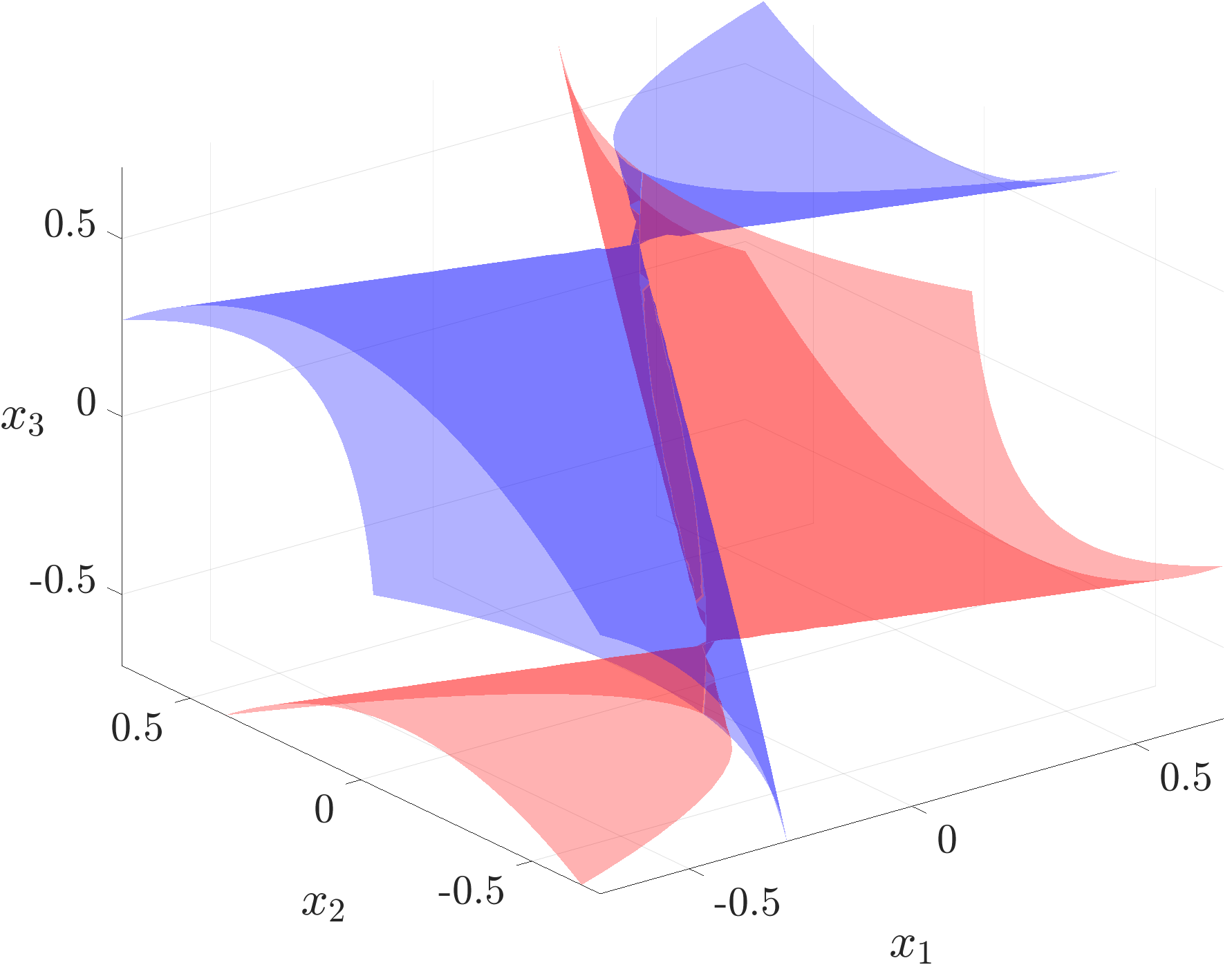
Likewise, for $d=3$ and $m=1$, Fig. 4(b) reveals that a generic line has $6$ intersections with the bounding real algebraic surfaces whereas from (48), we know that the polynomials $p^{\text{upper}},p^{\text{lower}}$ in this case, are of degree $4$. So the integrator reach set box-valued input set $\mathcal{U}$, is not a spectrahedron.

References

- [1] D. Maksarov and J. Norton, “State bounding with ellipsoidal set description of the uncertainty,” International Journal of Control, vol. 65, no. 5, pp. 847–866, 1996.
- [2] N. Kochdumpe, V. Gaßmann, F. Gruber, M. Klischat, B. Schürman, and M. Althoff, “AROC 2020 manual,” Technical University of Munich. [Online]. Available: https://tumcps.github.io/AROC/data/Aroc2020Manual.pdf
- [3] A. B. Kurzhanski and P. Varaiya, Dynamics and Control of Trajectory Tubes: Theory and Computation. Springer, 2014, vol. 85.
- [4] J. Lévine, P. Martin, and P. Rouchon, “Flatness and defect of non-linear systems: introductory theory and examples,” International Journal of Control, vol. 61, no. 6, pp. 1327–1361, 1995.
- [5] R. M. Murray, M. Rathinam, and W. Sluis, “Differential flatness of mechanical control systems: a catalog of prototype systems.” ASME International Mechanical Engineering Congress and Exposition, 1995.
- [6] J. Lévine, P. Martin, and P. Rouchon, “A Lie-Bäcklund approach to equivalence and flatness of nonlinear systems,” IEEE Transactions on Automatic Control, vol. 44, no. 5, pp. 922–937, 1999.
- [7] P. Varaiya, “Reach set computation using optimal control,” in Verification of Digital and Hybrid Systems. Springer, 2000, pp. 323–331.
- [8] S. Haddad and A. Halder, “The convex geometry of integrator reach sets,” in 2020 American Control Conference (ACC). IEEE, 2020, pp. 4466–4471.
- [9] D. Cox, J. Little, and D. OShea, Ideals, varieties, and algorithms: an introduction to computational algebraic geometry and commutative algebra. Springer Science & Business Media, 2013.
- [10] G. Zaimi, “A polynomial implicitization,” MathOverflow. [Online]. Available: https://mathoverflow.net/q/381335
- [11] H. S. Wilf, generatingfunctionology. CRC press, 2005.
- [12] L. Kronecker, Zur Theorie der Elimination einer Variabeln aus zwei algebraischen Gleichungen. Buchdruckerei der Königl. Akademie der Wissenschaften (G. Vogt), 1881.
- [13] R. Salem, Algebraic numbers and Fourier analysis. Wadsworth Publishing Company, 1983.
- [14] C. Vinzant, “The geometry of spectrahedra,” in Sum of Squares: Theory and Applications. American Mathematical Society, 2020, pp. 11–36.
- [15] S. Haddad and A. Halder, “The curious case of integrator reach sets, Part I: Basic theory,” arXiv preprint, arXiv:eess.SY/2102.11423, 2021. [Online]. Available: https://arxiv.org/pdf/2102.11423.pdf
- [16] J. Bochnak, M. Coste, and M.-F. Roy, Real algebraic geometry. Springer Science & Business Media, 2013, vol. 36.
- [17] J. W. Helton and J. Nie, “Semidefinite representation of convex sets,” Mathematical Programming, vol. 122, no. 1, pp. 21–64, 2010.
- [18] J. W. Helton and V. Vinnikov, “Linear matrix inequality representation of sets,” Communications on Pure and Applied Mathematics, vol. 60, no. 5, pp. 654–674, 2007.