Abstract
We study the generation of a large power spectrum, necessary for primordial black hole formation, within the effective theory of single-field inflation. The mechanisms we consider include a transition into a ghost-inflation-like phase and scenarios where an exponentially growing mode is temporarily turned on. In the cases we discuss, the enhancement in the power spectrum results from either a swift change in some effective coupling or a modification of the dispersion relation for the perturbations, while the background evolution remains unchanged and approximately de Sitter throughout inflation. The robustness of the results is guaranteed thanks to a weakly broken galileon symmetry, which protects the effective couplings against large quantum corrections. We discuss how the enhancement of the power spectrum is related to the energy scale of the operators with weakly broken galileon invariance, and study the limits imposed by strong coupling and the validity of the perturbative expansion.
IFT-UAM/CSIC-21-93
Large power spectrum and primordial black holes in the effective theory of inflation
Guillermo Ballesteros,a,b Sebastián Céspedes,a,b Luca Santonic
aInstituto de Física Teórica UAM/CSIC,
Calle Nicolás Cabrera 13-15, Cantoblanco E-28049 Madrid, Spain
bDepartamento de Física Teórica, Universidad Autónoma de Madrid (UAM)
Campus de Cantoblanco, E-28049 Madrid, Spain
cCenter for Theoretical Physics, Department of Physics,
Columbia University, New York, NY 10027
guillermo.ballesteros@uam.es, sebastian.cespedes@uam.es, luca.santoni@columbia.edu
1 Introduction
The idea that primordial black holes (PBHs) could constitute all the dark matter of the Universe or part of it has gained a remarkable momentum in recent years. The most popular scenario for the production of black holes in the primordial Universe consists in the collapse of radiation overdensities, which originate from large quantum fluctuations seeded during inflation, see e.g. Carr:1993aq; Ivanov:1994pa. Several models devised with the aim of enhancing the primordial spectrum have been recently explored. Most of them have a single inflationary field whose dynamics deviates from standard slow-roll, leading to a primordial spectrum peaking with a large value at some scale of (comoving) distance. See Ivanov:1994pa; Garcia-Bellido:2017mdw; Ballesteros:2017fsr; Cicoli:2018asa; Ozsoy:2018flq; Mishra:2019pzq; Ballesteros:2019hus; Ballesteros:2020qam for a representative sample of a popular class of models.
From a broader perspective, one can identify two physically distinct options that implement dynamical characteristics leading to large primordial fluctuations. The first possibility is a substantial change in the homogeneous background evolution of the Universe during inflation. Many concrete models that fall in this category—and in particular the ones mentioned above—feature a significant reduction of the slow-roll parameter . Rather generically, this can lead to a breakdown of the slow-roll evolution and, possibly, a transition into an ultra slow-roll phase Germani:2017bcs; Motohashi:2017kbs; Ballesteros:2017fsr. This kind of background dynamics induces a large effect in the small quantum fluctuations that are inherently associated to the background, generating a large primordial spectrum. A second possibility consists instead in some modification of the dynamics of the perturbations alone, while keeping the background evolution in a, rather featureless, inflationary evolution, see Ballesteros:2018wlw (and also Palma:2020ejf; Fumagalli:2020adf). In the present work, we will focus on this latter case, assuming a standard quasi-de Sitter spacetime during inflation, with approximately constant slow-roll parameters throughout.
For our analysis to be as general and model-independent as possible, we will work within the framework of the effective field theory (EFT) of single-field inflation Creminelli:2006xe; Cheung:2007st. In addition, the robustness of our results will be guaranteed by an approximate symmetry, which protects the effective couplings against potentially large quantum corrections. This is in contrast with the more commonly explored models, mentioned earlier, in which a large power spectrum comes from a very small . In such models, the smallness of generically arises as a consequence of a fine tuning of the parameters in the (covariant) Lagrangian of the inflaton. This tuning can be a cause of concern because it is in general not protected by any symmetry.
Besides our phenomenological motivation of PBHs as dark matter, the question of determining the largest primordial spectrum consistently allowed in the EFT of inflation from different operators is interesting on its own. Although a very large spectrum is physically irrelevant at large enough distance scales, due to stringent Cosmic Microwave Background (CMB) and Large Scale Structure (LSS) bounds, the size of the spectrum at smaller scales can be orders of magnitude larger. Indeed, even though there exist indirect, model-dependent and scale-dependent bounds (coming mainly from the absence of compelling evidence for the existence of PBHs), there are comoving scales where the primordial spectrum is essentially unconstrained. In particular, there are no bounds in the range Mpc – Mpc, corresponding to PBHs that would have formed during radiation domination with masses between and .11 1 See Green:2020jor; Carr:2020gox for recent compilations of PBH bounds.
In models that do not rely on a reduction of , a large primordial spectrum is usually accompanied by sizable interactions between fluctuations and significant non-Gaussianities. This means that the primordial spectrum cannot be arbitrarily large without stepping over the regime of validity of the EFT. For instance, the partial-wave unitarity cutoff for models with an inflaton featuring a Lagrangian of the form Armendariz-Picon:1999hyi and a small speed of sound is . The consistency requirement can then be rephrased as Cheung:2007st, setting a bound on the maximum primordial spectrum that can be achieved for a given (small) value of . Since in the simplest, Gaussian, approximation the PBH abundance depends (exponentially) on the primordial spectrum, the relation may be used to constrain mechanisms of PBH formation in scenarios in which is small Ballesteros:2018wlw. Assuming that a large is needed to generate an abundance of PBHs compatible with the dark matter density, it was argued in Ballesteros:2018wlw that mechanisms based on a small in the realm of the vanilla EFT of inflation—i.e. with the kind of covariant action mentioned above—point towards a very small and, possibly . This conclusion assumes small variations of the EFT coefficients during inflation, but it is nevertheless indicative of the difficulty of obtaining a large primordial spectrum in the EFT of inflation from a variation of ; a difficulty that becomes more severe as the desired spectrum is increased.
A potential way of circumventing this issue, which was already suggested in Ballesteros:2018wlw, consists in invoking a modified dispersion relation for the primordial fluctuations, as it happens e.g. in ghost inflation ArkaniHamed:2003uz. This changes the cutoff of the EFT through the appearance of a new scale, which is associated to the higher-dimensional terms of the action responsible for the modified dispersion relation. In the present paper we will explore this idea in more depth. One of main results of our paper is the following: we find that a transition into a phase of ghost condensation results in an enhanced power spectrum, while it raises the unitarity cutoff of the theory, which avoids the strong coupling issues arising from a small speed of sound and keeps the theory for the perturbations weakly coupled during the evolution. The enhancement of the primordial spectrum in this case is in the form of a power law and scales generically as , where represents the new raised cutoff.
To put the following discussion into context, we need to understand what we mean by a ‘large power spectrum’. As we mentioned before, the PBH abundance is exponentially sensitive to the primordial power spectrum, in the Gaussian approximation. It turns out that, with this approximation, is required in order for PBHs to account for all the dark matter. This is a crude approximation as it ignores several effects that may be important, depending on the model, notably: non-Gaussianities, stochastic dynamics, shape of the primordial spectrum, threshold for the formation of PBHs and equation of state of the Universe at the time of formation. For this reason, we will not focus our analysis on obtaining a specific value of , but rather on primordial spectra that are orders of magnitude larger than the CMB one, in a broad range. Nevertheless, we can still use as a convenient benchmark, keeping in mind that smaller values of —possibly orders of magnitude smaller—may be enough to account for all dark matter. In any case, (or any meaningful large value relevant in this context) is indeed very large in comparison to the primordial spectrum inferred from the CMB, which is about seven orders of magnitude smaller.
In order to explore the possibilities for obtaining a large primordial spectrum in the EFT of inflation away from a reduction in ,22 2 Often implying a large second slow-roll parameter in concrete models, see e.g. Ballesteros:2017fsr. we will focus on the operators and in the unitary gauge action for the perturbations Creminelli:2006xe; Cheung:2007st. Despite being higher order in derivatives, can become as large as on the inflationary background thanks to a weakly broken galileon (WBG) symmetry, in a way that is stable under loop corrections Pirtskhalava:2015nla; Santoni:2018rrx. The combination of these operators can make the sound speed become very small and the dispersion relation for the perturbations, which in general reads
| (1.1) |
dominated by the term (see Eq. (2.12) for the expressions of and in terms of the effective coefficients).
In addition to the transition into a ghost-inflation-like phase, we discuss another mechanism, which allows to increase more efficiently the power spectrum. This consists in pushing the sound speed beyond , allowing for a transient phase with . In this case, the primordial spectrum grows exponentially (at specific comoving scales).
As we will discuss, there is in principle nothing wrong with this temporary instability provided that the dynamics of modes with the largest physical momenta is controlled by the term. However, the validity of perturbation theory will restrict the duration of the phase with as well as the amplitude of the change in . Phases with this type of instability have been discussed before see e.g. Creminelli:2006xe, and more recently in Garcia-Saenz:2018ifx; Garcia-Saenz:2018vqf; Fumagalli:2019noh; Bjorkmo:2019qno; Ferreira:2020qkf; Palma:2020ejf; Fumagalli:2020adf; Fumagalli:2020nvq.
The paper is organized as follows. In Section 2 we review the EFT of the (scalar) fluctuations of a single scalar field coupled to gravity—during inflation and at quadratic order in the fluctuations—including the general next-to-leading order term in spatial derivatives, see Eq. (2.4). In Section 3 we discuss, using the EFT, to what extent it is possible to enhance the power spectrum by means of a negative friction coefficient in the linearized equation for the perturbations. In Section 4 we discuss how a transition from a standard phase with linear dispersion relation for the perturbations, , into a phase with quadratic dispersion relation, , can result in an enhanced primordial spectrum. In particular, we compare this enhancement to the one that can be obtained (within the EFT) from a swift change in the slow-roll parameters assuming .
In Section 5 we entertain the possibility that becomes temporarily negative during inflation, leading to an exponential enhancement of the perturbations. In Section 6 we discuss the relation between non-Gaussianities and the validity of the EFT. In Section 7 we present our conclusions. Appendices A and B deepen on various aspects of the main text, while we compare in Appendix C our findings to previous results in the context of multi-field models.
Conventions:
We work in mostly-plus signature for the metric, . The Hubble and slow-roll parameters are defined in cosmological time by , and . Throughout the paper we will declare that slow-roll is satisfied if , and higher order slow-roll parameters are . The conformal time is denoted with and is defined by . Comoving spatial momenta living in Fourier space are denoted in bold font as , and we define . The reduced Planck mass is .
2 Preliminary effective field theory considerations
Let us start from the EFT of a single scalar degree of freedom coupled to gravity in a FLRW spacetime, with background metric , in unitary gauge Creminelli:2006xe; Cheung:2007st (in which all the fluctuations are on the spacetime metric). Up to quadratic order in perturbations, we will focus on the following subset of operators:
| (2.1) |
where denotes the trace of the extrinsic curvature associated with the equal-time hypersurfaces of the spacetime foliation defined by the unitary gauge choice Cheung:2007st. The first line in (2.1) is unambiguously fixed by the background dynamics. The second line contains some of the quadratic operators that contribute to the action up to second order in the derivative expansion. The coefficients of these operators, such as , and are actually arbitrary functions of time, due to the breaking of time diffeomorphisms. In the absence of any other symmetries, higher derivative operators,33 3 By higher derivative operators we mean operators that in the covariant Lagrangian have more than one derivative per field (see Appendix A), or equivalently that in the unitary gauge language of (2.1) have at least one derivative acting on the metric perturbations. like and , are usually subleading and the dynamics of the perturbations at quadratic order is dominated by . In this paper, we are interested instead in situations where and are of the same order on the FLRW background. At first sight, this seems in contrast with the spirit of the EFT. However, as shown in Pirtskhalava:2015nla; Santoni:2018rrx, having (and hence both operators of the same order) is possible in theories characterized by a WBG invariance. As a bonus, a non-renormalization theorem, stemming from the weakly broken symmetry, guarantees that quantum corrections to and are parametrically suppressed. For further details on models featuring a WBG symmetry, see Appendix A.44 4 In principle, there are other operators in (2.1) that we did not write that belong to the same class of operators with WBG symmetry. However, thanks to the non-renormalization theorem, it is completely safe to set their tree-level couplings to ‘zero’ in (2.1). The operator is instead of a different type. It is not protected by symmetries and it is always subleading compared, e.g. to in the Lagrangian.55 5 Unless it enters through the combination , which also belongs to the class of Horndeski operators with WBG symmetry Pirtskhalava:2015nla. Nevertheless, it may end up providing the leading correction to the dispersion relation for the perturbations ArkaniHamed:2003uy; ArkaniHamed:2003uz; Baumann:2011su.66 6 As we will see, this can happen as a result of cancellations between different coefficients in the dispersion relation. However, this is not a fine tuning thanks to the WBG symmetry. Since we will discuss this option in the following, we have written explicitly this operator in (2.1). Note however that there are other operators of the same type that enter at the same order in derivatives and that, in principle, we should have written in (2.1). In fact, these operators are generated via loop corrections from the ones in (2.1). We have omitted them for simplicity because they do not change our results qualitatively. In this sense, should be considered as a representative of this class of operators. To recap, we will focus below on the action (2.1) where the effective couplings satisfy the following hierarchy,77 7 Notice that is the only relevant scale for the size of (massless) metric fluctuations during inflation. Therefore, since has dimension of mass 1, its expected order of magnitude is on purely dimensional grounds.
| (2.2) |
which is stable against quantum corrections.
To study the dynamics of the scalar perturbations it is convenient to use the -gauge, defined by Maldacena:2002vr:
| (2.3) |
After integrating out the non-dynamical components of the metric, and , from (2.1), one finds the following quadratic action for ,
| (2.4) |
where
| (2.5) | ||||
| (2.6) | ||||
| (2.7) |
being
| (2.8) |
The possible values for the coefficients are restricted by the validity of the effective description (see, e.g., Pirtskhalava:2015nla; Santoni:2018rrx and Appendix A below):
| (2.9) |
where . To make our expressions simpler, we will work in the decoupling limit (i.e. the regime where the scalar mode is decoupled from the metric perturbations Cheung:2007st),88 8 To explore the whole range of values for the parameters in (2.9), one would need to take into account the coupling to the metric perturbations. However, this would not change qualitatively our conclusions, but it would complicate unnecessarily the expressions for , , etc.. which applies if Pirtskhalava:2015nla
| (2.10) |
Using (2.10), Eqs. (2.5)–(2.8) simplify considerably and the quadratic action for reduces to
| (2.11) |
where now
| (2.12) |
Note that, even if the decoupling limit applies in the whole range (2.10), in the following we will mainly assume
| (2.13) |
which corresponds to cases where the inflationary background dynamics is mostly driven by the scalar’s potential Pirtskhalava:2015nla; Pirtskhalava:2015zwa. If this latter hierarchy is satisfied, then99 9 We stress again that the effective theory (2.1) will contain in general other operators of the same type of (even if we did not write them explicitly in (2.1)) that contribute to in (2.11) (and enter at the same scale of ). These will change the explicit expression of in (2.12), but will not change its dependence on the relevant scales of the problem, Eq. (2.14), which is what we will be using in the following.
| (2.14) |
where we defined the scale as
| (2.15) |
In theories with a WBG invariance, is precisely the scale that suppresses the higher derivative operators; see, e.g., Pirtskhalava:2015nla; Pirtskhalava:2015zwa and Appendix A below.
Note that in (2.11) the quadratic operator is the first of a series of terms of the form . We did not write explicitly these operators for because, as required by the consistency of the derivative expansion, they are increasingly subleading at low (comoving) momenta as grows, provided that
| (2.16) |
where is the conformal time and where we used the slow-roll approximation to write . Thus, at any given , only modes with comoving momentum satisfying (2.16) are captured by the derivative expansion (2.1). If , Eq. (2.16) ensures that all the operators with provide subleading corrections to the linearized scalar dynamics. However, it may happen that the system dynamically evolves into a phase in which . In this case, the operator may become the leading one, changing the dispersion relation for . If this happens before the dynamics becomes strongly coupled, then the system effectively enters a ghost-condensate-like phase ArkaniHamed:2003uy; ArkaniHamed:2003uz. In the following, we will discuss precisely this situation and analyze to what extent this can be used to enhance the power spectrum of within the EFT (2.1).
2.1 Linearized mode function equations
It is convenient to rewrite the linearized equation of motion for in terms of the number of e-folds , which are related to the cosmological time and the conformal time through
| (2.17) |
Defining
| (2.18) |
where
| (2.19) |
mirroring the notation of Pirtskhalava:2015zwa, the quadratic action for (2.11) can be rewritten as
| (2.20) |
where the prime denotes derivatives with respect to the conformal time . Then, one finds the following Mukhanov–Sasaki type of equation for the mode function in momentum space,
| (2.21) |
Throughout the paper, we will use the following definition for the first two slow-roll parameters:
| (2.22) |
In addition, we define
| (2.23) |
We will say that generalized slow-roll is satisfied provided that , , higher order slow-roll parameters and , are . With this notation,
| (2.24) |
and the equation (2.21) takes the form
| (2.25) |
or, equivalently, in terms of ,
| (2.26) |
Setting in (2.12) (which means ) and (which implies , and ) we recover the analogous equation studied in Ballesteros:2018wlw (setting there ). Later on, we will discuss particular solutions to (2.26) and compute the corresponding power spectra, which we will compare to the slow-roll one. Neglecting for the time being the -term in the dispersion relation (), at leading order in generalized slow-roll, the power spectrum for is
| (2.27) |
which in the aforementioned limit () reduces to the usual expression for :
| (2.28) |
2.2 Strong coupling
As in any EFT, a fairly reliable way to determine the regime of validity of (2.1) is to estimate the energy scale at which the theory becomes strongly coupled or perturbative unitarity breaks down. To this end, one would need to include in (2.1) all the interactions that contribute at the same order in derivatives, e.g. the cubic operators and (which we did not write explicitly in (2.1)), and determine for instance at which energy scale loop corrections become as large as the tree-level diagrams. As an example, we consider below the operator , which results from . This will be particularly relevant later on, when we consider the case of small . Indeed, when , different operators provide in general different estimates of the strong coupling scale. In particular, in the limit , the operator is the first one to become strongly coupled Cheung:2007st; Senatore:2009gt; Pirtskhalava:2015zwa.
Let us start considering the limiting case , with . If the EFT coefficients are constant in time, or at least do not change too fast—more on this point later—, following e.g. Pirtskhalava:2015zwa, one finds
| (2.29) |
where we have used the expression (2.15) for and we have defined
| (2.30) |
It is sometimes convenient to rewrite (2.29) in terms of the slow-roll power spectrum (2.27),
| (2.31) |
Requiring that amounts to the condition
| (2.32) |
Similar conditions can be obtained from other interactions in the EFT (2.1). Let us assume that initially and are all . If or then decrease in time, the left-hand side of (2.32) becomes smaller, while the power spectrum on the right-hand side increases according to (2.27). The system approaches therefore strong coupling, resulting eventually in a breaking of the effective expansion once (2.32) ceases to hold. When goes to zero, the breakdown of the effective theory can be avoided if, before strong coupling is reached, the operator becomes dominant over resulting in a change of the dispersion relation Baumann:2011su. In this case, the system effectively enters a ghost-condensate phase ArkaniHamed:2003uy; ArkaniHamed:2003uz, which provides a weakly-coupled UV completion Baumann:2011su. In this new phase, the strong coupling scale, determined by the operator , is precisely1010 10 Had we chosen the operator instead of to determine the strong coupling scale, we would have found (assuming again ) instead of (2.33), in agreement with Eq. (3.25) of Baumann:2011su.
| (2.33) |
where we used (2.13) and (2.14), dropped numerical factors and assumed for simplicity.
To derive (2.29) and (2.33) we have assumed that all the EFT couplings are (approximately) constant. In general, this is allowed if the typical energy scale associated with the time dependence in the effective couplings, , is smaller than . Indeed, the rate of change of some effective coupling over a Hubble time can be estimated as , which will be much smaller than itself—i.e. the variation is slow—provided that . However, in the following we will be interested in considering situations where some of the parameters, in particular and , change over time scales that are smaller than . Can this affect the estimate of the range of validity of the EFT, invalidating in particular (2.29) and (2.33)? In principle, these will remain good estimates of the strong coupling scale as long as the typical time scale associated with the time evolution of these coefficients, , is larger than . In the presence of such a scale separation, it is acceptable to estimate the strong coupling scale of the theory—which effectively corresponds to probing the short-distance dynamics of the perturbations in the system—as if the effective coefficients were constant in time. In terms of the number of e-folds, requiring that the time scale of a certain ‘feature’ in the effective coefficients or the power spectrum is much larger than (which can be thought of as the ‘time-resolution’ of the EFT) amounts to the condition , where we assumed . Under this assumption, one can rely on (2.29) and (2.33) to estimate the regime of validity of the effective theory. The presence of the feature might affect the value of by at most an correction, but it will not change its order of magnitude.
3 Enhanced power spectrum from negative friction
In this section we discuss one of the possible mechanisms by which a large power spectrum can be obtained in the EFT (2.1). This consists in the excitation of a growing mode when it is outside the horizon because the Hubble friction in the linearized equation for becomes negative. This mechanism has been studied in the literature when the change of sign in the friction comes from either (see e.g. Ballesteros:2020qam and references therein) or the time variation of the speed of sound (see Ballesteros:2018wlw; Ozsoy:2018flq). Here we will consider a variation of the EFT coefficient —see Eq. (2.23)—which encompasses also the latter of those.
Let us first consider Eq. (2.26) in the small- limit. One of the two possible solutions of this equation is simply , which (using the appropriate boundary conditions) gives the expression (2.27) for the power spectrum if the variation of the EFT coefficients is slow. The other solution satisfies
| (3.1) |
If the sign of the ‘friction coefficient’ , defined by
| (3.2) |
becomes negative during inflation, is not conserved on superhorizon scales and its spectrum may grow significantly above the slow-roll solution (2.27). This friction enhacement of the spectrum can arise from a fast change in which temporarily triggers (see, e.g., Ballesteros:2017fsr; Ballesteros:2020qam; Ballesteros:2020sre). We are instead interested in the possibility of , with small and approximately constant and . From Eq. (2.23) we see that can occur if diminishes fast enough. In particular, an reduction of over one e-fold is necessary for this friction enhancement to take place. Assuming a sudden change of to a value that remains constant over a time interval to decrease rapidly afterwards, the maximum enhancement can be estimated as
| (3.3) |
where is given by (2.27). We emphasize that this effect is different from the enhancement that can happen from a slow decrease of , which is already explicit in (2.27).
The exponential enhancement (3.3) is in principle possible, but we should check that it does not violate perturbative unitarity in the EFT, nor any of the assumptions in Section 2.2. In particular, we will require that (2.29) is valid and that the inequality (2.32) is satisfied. For simplicity, let us start assuming constant—we shall discuss later cases where evolves in time. Plugging (2.27) into (2.32) and assuming initially, one infers that cannot get smaller than roughly . In other words, defining , weak coupling requires roughly , if is initially close to zero. On the other hand, in order for the friction coefficient (3.2) to become negative, one needs . Combined with , this implies . However, from the considerations in Section 2.2, we want to trust (2.29) in the first place. Therefore, one concludes that, even if it is certainly possible to obtain a significant enhancement of the power spectrum by means of a large and negative , this may require some additional assumptions about the UV physics. Otherwise, based on the results of Section 2.2, the enhancement is bounded by the combined requirements that becomes not too small and its variation is not too fast.
We consider an explicit example in Figure 1, where we show the power spectrum for a particular choice of the time evolution of the coefficient . In the figure, decreases from an number by roughly orders of magnitude, in a time lapse of a couple of e-folds, before increasing again back to its original value.1111 11 In this example is constant for simplicity. This is possible in spite of the change in (required to have a variation of ), thanks to the freedom in the choice of , see Eqs. (2.12). As a result, this translates into an enhancement of the power spectrum of about four orders of magnitude, with respect to the CMB value, which has been set at to be .
It is instructive to compare the previous case to the one in which . As we mentioned at the end of Section 2.1, if then and . In this case, assuming a slow variation of the EFT coefficients, and a reduction of enhances the slow-roll spectrum. However, when (assuming ) and such a variation cannot enhance the spectrum by means of the friction effect discussed above, as it only makes the non-constant mode of fall even more rapidly as grows. The enhancement of the power spectrum from a change in was discussed in Ballesteros:2018wlw in analogous terms. There, it was pointed out that a small sound speed, leading to a large (as required for abundant PBH formation) can lead to strong coupling and the loss of validity of the effective theory. In that case, the strong coupling condition (2.32) reduces indeed to Creminelli:2006xe, which provides a lower bound on . In the following, we we will explore further the possibility of enhancing the power spectrum through a change in the sound speed, as well as possible ways to avoid strong coupling issues.
4 Enhanced power spectrum from a ghost-inflation phase
In Ref. Ballesteros:2018wlw it was pointed out in the context of PBH formation that the strong coupling problem that arises when one tries to enhance the power spectrum to large values by sending may be addressed by considering a modified dispersion relation in this limit, and specifically the case of ghost inflation ArkaniHamed:2003uz.1212 12 Another possibility consists in invoking the appearance of new degrees of freedom that provide a UV completion to the effective theory, see Appendix C. This is because a change in the dispersion relation for the low-energy degrees of freedom can raise the cutoff of the theory, extending the regime of validity of the effective description. In the following, we discuss in detail this possibility. In particular, we consider the case in which the system transits from a slow-roll regime into a ghost-condensate-like phase. This is possible provided that is appropriately chosen. The robustness of the transition is ensured by the assumed WBG symmetry Pirtskhalava:2015nla; Pirtskhalava:2015zwa. As we will see, this type of transition, which modifies the dispersion relation for the perturbations, allows to simultaneously enhance the power spectrum on shorter scales and keep the theory for the perturbations weakly coupled during the evolution.
The initial slow-roll evolution is characterized by the usual dynamics (with initially),
| (4.1) |
which admits the standard solution
| (4.2) |
where the Wronskian condition has been imposed at . As decreases in time, the slow-roll power spectrum (2.27), obtained from the solution (4.2), increases, but at the same time the system approaches strong coupling. However, before it becomes strongly coupled, we assume that the dynamics of the perturbations gets dynamically modified, in particular that the term proportional becomes dominant over in Eq. (2.21):
| (4.3) |
Given a certain mode with momentum , the crossover between the two regimes occurs at the conformal time , defined by . Modes with very small that exit the horizon very soon will not be affected by the change in the dynamics, and will have the power spectrum given in (2.27). Let us focus instead on modes with larger , that were still sub-horizon during the transition into the ghost-inflation like phase. In order to estimate the power spectrum for these modes, we can proceed as follows. First, we solve the mode function equation (4.3). The most general solution can be written as ArkaniHamed:2003uy; ArkaniHamed:2003uz
| (4.4) |
Next, we match (4.4) to (4.2) by requiring continuity across the transition. This will unambiguously fix the coefficients and in (4.4). Since the modes which we want to estimate the power spectrum for after the transition were well within the horizon in the slow-roll phase, we can obtain a reasonable approximation to the solution in the ghost-condensate phase by matching (4.2) and (4.4) at large negative conformal times, .1313 13 Clearly the correct procedure would require matching and at the crossing point—see, e.g. Figure 2 below. However, doing this does not significantly affect the order of magnitude of the enhancement in (4.10). Using the following formulae for the Hankel functions,
| (4.5) |
and keeping only the solution proportional to in (4.4), which has the correct phase at short distances, we can approximate
| (4.6) |
By definition, at the transition one has . Then,
| (4.7) |
and the matching with (4.2) yields
| (4.8) |
Expanding at , one finds the following estimate for the power spectrum after the transition,1414 14 We stress that (4.9) holds only in the limit of very large . Keeping finite introduces corrections that depend on and computed at . A more precise realization of the transition is discussed later, with the resulting power spectrum shown in Figure 2.
| (4.9) |
to be compared with the slow-roll power spectrum (2.27), which gives
| (4.10) |
where is the sound speed in the slow-roll phase before the sound speed starts changing in time. If we take before the transition, then it follows from (4.10) that the final power spectrum is enhanced by a factor of (recall that ) for modes that exit the horizon after , with respect to modes that become super-horizon during the slow-roll phase.
In order to understand the origin of the enhancement, we shall reason as follows. It is convenient to focus on the two-point functions resulting from the solutions (4.2) and (4.4) as functions of . In particular, let us assume for simplicity that is the only time-dependent quantity, with initially, while all the other parameters are constant, and let us define the functions and , where . is related to the power spectrum (2.27) in the slow-roll phase via , while gives, in the limit , the power spectrum (4.9) in the ghost-condensate phase after multiplying by the same overall constant and using (4.8). As already mentioned above, modes with momentum that exit the horizon well before the sound speed starts decreasing will not be affected by the change in the dynamics and will have a power spectrum determined by with . Instead, the power spectrum of modes that become super-horizon while is decreasing (but before their dispersion relation switches from linear to quadratic) is still determined by but with a smaller value for . In particular, the enhancement of these modes with respect to the previous ones scales (in the slow-roll approximation) as at horizon crossing, as dictated by Eq. (2.27). Finally, let us consider modes with values of that exit the horizon in the ghost-condensate phase. These modes are still sub-horizon around . Before , their amplitude follows (up to an overall constant factor) the curve as a function of , while after they will evolve according to . However, since and have different shapes in , and, in particular, since decreases more slowly than , the power spectrum is larger than what it would be without the change in the mode dynamics. The enhancement scales precisely as . We emphasize that this precise scaling holds strictly speaking in the limit of very large . Considering a shorter duration for the ghost-inflation-like phase will in general translate into a smaller enhancement. In addition, the actual enhancement in the power spectrum will also depend on the details of the transition and on the presence of oscillations, which may result in a larger peak. We show an explicit example in Figure 2, where we plot . In the left panel, we have assumed that the system is initially in a slow-roll phase with and negligible. At some time in the evolution, goes to zero and the dynamics becomes thereafter dominated by the -term.1515 15 In reality, will never be exactly zero. It is indeed bounded from below by the size of the quantum corrections to the effective couplings in (2.12). As shown by the orange dashed line, the slope of the spectrum goes as . Note that this is the same slope that was found in Byrnes:2018txb, although the growth there is due to a change in the background evolution (in particular, a transition into an ultra-slow-roll phase) instead of a change in the dispersion relation for the perturbations. In the right panel, the evolution is the same except that the phase with quadratic dispersion relation has finite duration: e-folds after the first transition, the sound speed becomes again, and the initial slow-roll dynamics is restored. To make the analysis as simple as possible, we have assumed the transitions between the different phases instantaneous, and we have matched the solutions for and at the transition points.

Looking at Eq. (4.10), one might be tempted to conclude that, by suitably choosing to be sufficiently small (which, using the scaling (2.14), would correspond to raising the scale ) it is possible to obtain an arbitrarily large relative enhancement of the power spectrum with respect to the standard slow-roll one. Nevertheless, we know that cannot be arbitrarily small (or, arbitrarily large—see Appendix A for further details). Indeed, a nonzero is generated anyway at the quantum level. Then, the relevant question is whether the possible values of that are compatible with the size of its quantum corrections allow to obtain the desired enhancement. Note that, according to (4.10), a relative increase of roughly or orders of magnitude would require of order . This seems hard to get using the values in Table 1 in Appendix A for the effective couplings (even in the kinetically-driven scenario) and the typical values of during inflation. However, one might get such small numbers for if the parametric separation between and is larger than the one we considered here (see Eq. (2.13)), which would correspond to further suppressing the relative size of the higher derivative operators with respect to standard operators in the theory. However, as mentioned above, oscillatory features such as those displayed in Figure 2 may lead to a larger spectrum (possibly by a couple of orders of magnitude) for a given , depending on the specific implementation of the transition into the ghost-condensate-like phase.
To recap, a phase with a quadratic dispersion relation () allowed us to attain two main results at the same time: firstly, it raised the cutoff of the theory, avoiding short modes (with large ) to become strongly coupled as ; secondly, it resulted in an enhanced power spectrum at large , compared to the power spectrum at low , thanks to a different time evolution for the modes in the slow-roll and ghost-inflation phases. The enhancement scales as , with bounded from below by the size of the quantum corrections in the theory. In the case of interest, the typical value of can be read off Eq. (2.14) and Table 1 in Appendix A.
5 Transition into a phase with imaginary sound speed
5.1 Exponential growth from ghost inflation
A transition into a ghost-inflation-like phase allowed us to alleviate the strong coupling regime that stems from reducing the sound speed of the perturbations and, at the same time, to enhance the power spectrum on short scales. However, since the relative increase is a power law in (in particular scales as ), an enhancement of seven orders of magnitude (as required by the Gaussian approximation to account for all DM with PBHs formed during radiation domination)1616 16 We reiterate that this approximation is unlikely to be precise given that it may not describe well enough the tails of the probability distribution function of . Still, a large power spectrum of is certainly needed for a large PBH abundance. is only possible at the price of further increasing the parametric separation between and , which is tantamount to pushing the form of the theory toward a standard theory. A different, and in principle more efficient, way to enhance the power spectrum is to excite a growing mode by assuming that, after transiting into the ghost-condensate phase, the quantity in (2.12) keeps decreasing and eventually becomes negative. This corresponds to an instability for the perturbation , which now grows exponentially. Usually, this is an unwanted behavior for the perturbations, as this sort of instability heralds a breakdown of the perturbative expansion and threatens the validity of the background classical solution. In the following, we will discuss to what extent such a gradient instability can be used to enhance the power spectrum in a controlled way over a period of time of a few e-folds. Caveats and possible obstructions are discussed later in this section and in Section 6.
We remain agnostic about the UV mechanism that is responsible for the exponential growth of the perturbations in the effective theory. In particular, we do not rely on any specific multi-field model.1717 17 In Fumagalli:2019noh; Bjorkmo:2019qno; Ferreira:2020qkf; Garcia-Saenz:2018ifx (see also Fumagalli:2020adf; Fumagalli:2020nvq and Appendix C) a gradient instability arises as a consequence of a transient tachyonic instability in a two-field model. In these works, a heavy degree of freedom becomes temporarily tachyonic. Once integrated out, the tachyonic phase manifests as a gradient instability in the infrared dynamics. In our analysis, the transition from the slow-roll phase into a transient regime of exponential growth is entirely captured by the weakly coupled, single-field effective theory (2.1) and it is driven by higher derivative operators with WBG symmetry Pirtskhalava:2015nla; Santoni:2018rrx. The robustness of the classical trajectory and of the EFT is guaranteed by the approximate symmetry, which protects the effective couplings against large quantum corrections.1818 18 See also Garcia-Saenz:2018vqf for a multi-field motivated EFT description of the gradient instability, albeit without any discussion about the role of the higher derivative operators (responsible for a modified dispersion relation at large momenta) or any symmetry considerations.
For the moment, let us start by focusing on the transition between the ghost-condensate regime and the phase with imaginary sound speed. Later on, we will consider a more complete scenario, in which these are transient phases in a more general inflationary slow-roll evolution.
In the ghost-condensate phase, the sound speed is effectively negligible and the linearized dynamics for the perturbations is described by (4.3). After this phase, we assume that evolves from zero to negative values. The dynamics is now governed by the mode equation
| (5.1) |
which corresponds to (2.21) at the leading order in the quasi-de Sitter approximation and where we replaced, for convenience, in such a way to work with positive . In general, the equation (5.1) cannot be solved exactly in the presence of a non-trivial time dependence in and . Therefore, we will take them constant and approximate the evolution with a sharp transition from a ghost-condensate phase (with and ) to a gradient-instability phase (with and ). We will thus solve the equation separately in the two phases, and match the solutions at the crossing point. To this end, let us define to be the (conformal) time when the transition takes place. In the ghost-condensate phase, , the term dominates in (5.1) and the solution is given by
| (5.2) |
where the standard boundary condition for ghost inflation has been imposed at ArkaniHamed:2003uz. After the transition time , the term dominates in (5.1) and the most general solution for takes the form
| (5.3) |
The coefficients and can be obtained by matching to (5.2), requiring the continuity of and across the transition point:
| (5.4) | ||||
| (5.5) |
where we used . These expressions can be further simplified using . Expanding the Hankel functions as in (4.5) for , we find
| (5.6) | ||||
| (5.7) |
Plugging these expressions back into (5.3), the power spectrum for is
| (5.8) |
where we used (2.18) and neglected subleading terms in . Eq. (5.8) can also be written as
| (5.9) |
where (normalized to the CMB measurements) corresponds to the power spectrum of the modes that exited the horizon before the instability phase (i.e. during the ghost-inflation phase). From (5.9) one can thus read off the enhancement factor , where we defined . In principle, it is enough to choose and in such a way that to obtain an enhanced spectrum as large as . Note that the power spectrum (5.9) is analogous to the one that arises from the tilted version of ghost inflation Senatore:2004rj. Yet, there are differences worth remarking. As opposed to Senatore:2004rj, where the growth of the perturbations stems from an increasing in time, which violates the Null Energy Condition (NEC), in our case the background evolution is not altered with respect to standard slow-roll inflation, i.e. with and . Instead, the instability that leads to a growth of the primordial perturbations is triggered by higher derivative operators in the underlying theory with WBG symmetry, resulting in a temporary change of the sign of (which we have approximated as an instantaneous transition).
It is worth stressing that (5.9) gives the maximum enhancement of the power spectrum. Recall indeed that we have confined our discussion so far to a single mode , while one should note that not all the modes experience the same relative enhancement. This will be transparent in the next section (see, in particular, Figure 3), where we consider an analytic approximation for the transient unstable phase and analyze in more detail the behavior of the different modes during the evolution.
5.2 Analytic approximations for the transition into the unstable phase
In this section, we consider a more refined version of the dynamics we just discussed above. In particular, we assume that the system evolves from a slow-roll phase into a transient unstable phase dominated by a dynamics for the perturbations with . Then, after some time, turns positive again and the system recovers a slow-roll type of evolution. To make this scenario tractable analytically, we approximate the evolution by three separate phases, connected by instantaneous transitions, where the solutions to the equations of motion for the perturbations are matched. This will allow us to show explicitly the behavior of the different modes. A smoother version of the evolution is discussed in the next section, but all the main ingredients and qualitative aspects are already captured by the present stepwise approximation.
Let us start assuming that is the only time-dependent function determining the dynamics of the perturbations, while we will keep for simplicity all the other slow-roll parameters, including in (5.1), constant. To make the analysis as simple as possible, we will assume that changes instantaneously from a certain constant value to another constant value. In particular, we shall define and such that , and , where and . In the first phase defined by , the scalar perturbations have a standard dispersion relation with sound speed . In particular, the -term in (5.1) is subdominant for all the modes captured by the effective description. Then, the system undergoes a transient unstable phase triggered by for , and the amplitude of (some of) the modes increases exponentially. In the last phase starting at , the original value of the sound speed is restored and the modes stop growing. To understand the effect of the instability on the power spectrum, it is convenient to follow the evolution of modes with different momenta . Let us call the conformal time at which a certain mode with momentum exits the horizon. Modes with sufficiently small , i.e. , that exit the horizon before the unstable phase, i.e. , do not feel the effect of the gradient instability and will not have an enhanced power spectrum. Let us then focus on modes that exit the horizon during or after the unstable phase, i.e. such that . These will in general grow because of the instability and will have a power spectrum enhanced (with respect to the previous ones) by a factor of , where or , whichever is the smallest. This seems to indicate that the modes with the largest enhancement are the ones with the largest momentum. However, this comes with a caveat. One should take also into account the presence of the -term in (5.1), which can be relevant in the unstable phase since . Indeed, modes with large enough , in particular those with , whose dynamics resembles the one of ghost inflation, will not be significantly affected by the instability and will not grow as much as those with intermediate . Thus, the largest relative enhancement at the level of the power spectrum is obtained for modes with , and corresponds to , where we assumed .1919 19 Note that this estimate reproduces the exponential factor in (5.9) in the limit . An explicit example is shown in Figure 3, where we plot the power spectrum as a function of , normalized to the CMB value, , at .2020 20 Assuming the scaling (2.13) for (see also Table 1 in Appendix A), with the chosen value for defined in (2.12), to have the power spectrum in Figure 3 correctly normalized at to the CMB value, one needs . The plot has been obtained by solving the equation (4.1) with for and , and the equation (5.1) with for , and then matching and across the transition points. The shape with a peak at intermediate is in agreement with the numerical solution of Section 5.3. Note that the oscillations in Figure 3 follow from interference effects resulting from the transition between different phases Ballesteros:2018wlw.2121 21 We stress that this is true for all the oscillations visible in Figure 3, except those at the rightmost part of the plot. These ones are instead affected by the fact (with being the initial time where the boundary condition is imposed) is no longer the correct initial condition for modes with very large .
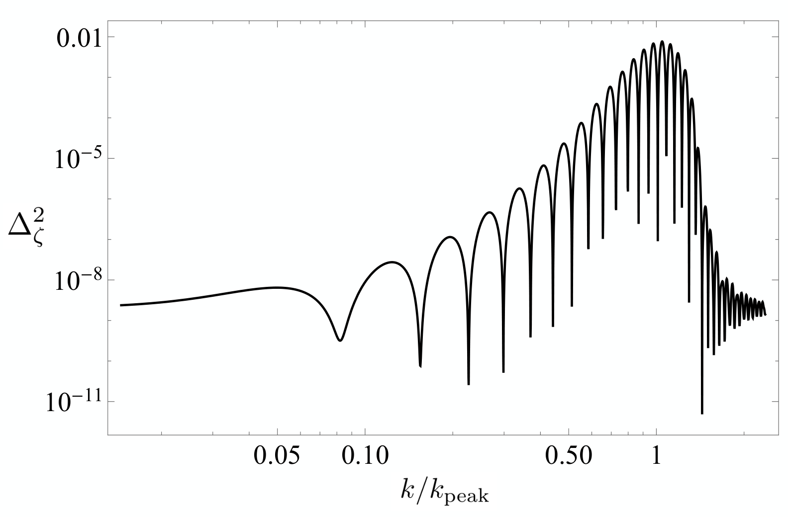
5.3 Numerical solution
In this section, we present a numerical solution to the equation (2.21) for a smoother version of the transition described in the previous section. The result is reported in Figure 4. To obtain the solution, we choose , with before and after the transition, while throughout the entire evolution. We assume that the system starts in a phase of slow-roll evolution and that the dynamics of the perturbations is initially governed by a standard dispersion relation with , as displayed in the right panel of Figure 4 (solid line). Then, the sound speed gradually diminishes and, after a couple of e-folds, the system enters the ghost-condensate-like phase with quadratic dispersion relation. The dashed curve in the right plot of Figure 4 describes the evolution of the EFT coefficient . Thereafter, the system temporarily stays in a phase with . This triggers an exponential growth of the amplitude of the perturbations, resulting in an enhanced power spectrum as shown in the left plot of Figure 4. Afterwards, returns positive restoring the original dynamics.
In the plot in Figure 4, one recognizes the two salient features discussed in Sections 5.1 and 5.2: the first one is the exponential enhancement obtained during the unstable phase (as opposed to the example in Figure 2 where the growth is compatible with a power law); the second one is the sudden decay in the shape of the power spectrum after the peak. The presence of the plateau before the exponential growth simply follows from the fact that modes with sufficiently small , which exit the horizon very soon, remain unaffected by the instability. The second plateau, occurring after the peak (and barely shown in the plot), arises instead, as noticed already in Section 5.2, because modes with very large remain dominated by the quadratic dispersion relation during the transient phase with . Therefore, they effectively remain in the ghost-condensate-like regime and are also not enhanced. As a result, the final power spectrum is peaked only over a finite range of momenta, which are those that effectively experience the gradient instability.
At this point, one might worry about the consistency of the effective expansion in the unstable phase and, in particular, across the points where the dispersion relation for turns from positive to negative, and vice versa. A prototypical example of the instability is the (an)harmonic oscillator in quantum mechanics with inverted potential. Let us imagine that the curvature of the potential is initially positive and that the oscillator is in its ground state. At some time, the curvature of the potential suddenly turns negative. In the limit of an instantaneous transition, the system will initially still be in the same state, but the wavefunction will start to change in time: it will grow and spread as a result of the unbounded potential. However, as long as the unstable phase is just temporary—one can imagine that, after a certain time interval, the curvature of the potential becomes positive again—the wave function will stabilize. In the case of an EFT with transient gradient instability, one should check that the maximum rate of the instability lies within the realm of validity of the effective expansion. In particular, focusing on the dispersion relation in the unstable phase, which we can write schematically as
| (5.10) |
the maximum rate of the instability is given by
| (5.11) |
where we used (2.14). Taking now into account Eq. (2.33) and that in the unstable phase, from (5.11) one finds that , corresponding therefore to energies that are below the cutoff.2222 22 This is correct if the loop corrections are dominated by the high-energy part of the loop integral, i.e. by the dynamics of modes with quadratic dispersion relation, , which are perfectly stable and weakly coupled. However, it does not completely address the question of strong coupling in the unstable phase. A quick scaling argument, following the one in the next section, seems to suggest the presence of potentially dangerous large -loop corrections in the large- limit, where the leading contribution comes from the exchange of exponentially growing modes. We leave a more detailed analysis of this aspect for future work. Finally, another possible obstacle in applying the EFT to describe the transition between slow-roll inflation (or the ghost condensate) and the unstable regime is that a too fast evolution may jeopardize the estimate of the strong coupling scale across phases—see our discussion in Section 2.2 above. On the other hand, this obstacle may not be insurmountable as long as one does not need to resolve the details of the transition between the two phases. Since we are mainly interested in the computation of the global shape of the power spectrum, we can still use the EFT to describe the relevant phases, whose robustness is guaranteed by symmetries, and match across the transition points, as we already schematically did before in the previous section.
6 Non-Gaussianities and the validity of perturbation theory
The main reason that has recently motivated the study of inflationary scenarios with large power spectra on small scales is the possibility of generating PBHs. Analytical and numerical analyses indicate that is needed for PBH formation. Therefore, in order to correctly estimate their abundance, the information about the size of the two-point function may not be enough, and one may need to know additional information about the full shape of the distribution, e.g. the form of higher-order correlation functions. The most promising approach to this issue may lie on techniques that attempt to go beyond perturbation theory, see e.g. Panagopoulos:2019ail; Ezquiaga:2019ftu; Figueroa:2020jkf; Pattison:2021oen; Celoria:2021vjw; Biagetti:2021eep for several recent attempts with different methods. Our goal in the present section is more modest. We will estimate the size of the leading -point correlation function for the example presented in the previous section and compare it with the power spectrum via the relation
| (6.1) |
which may give an indication of the validity of the perturbative expansion.
The presence of an (even temporary) instability inducing an exponential growth of the curvature perturbations may be worrisome, as it may yield even larger effects at the level of higher-point correlators, indicating the breakdown of perturbation theory. The actual situation is, however, less catastrophic. Refs. Bjorkmo:2019qno; Fumagalli:2019noh have shown indeed that, during a gradient instability phase, higher-point correlation functions of grow less than the naive counting based on the scaling of the field would suggest. In the present section, we briefly summarize this result and extend it to the case of the interactions resulting from the operators in the effective theory (2.1).
A generic -point correlation function can be computed in the in-in formalism Weinberg:2005vy as
| (6.2) |
where represents an insertion of the interaction Hamiltonian. After the Wick contractions of the fields, each nested commutator corresponds to the imaginary part of the product of a certain number of mode functions with an equal number of complex conjugate modes . Since, from (5.2), (5.6) and (5.7), the mode function for the curvature perturbation in the unstable phase is schematically of the form
| (6.3) |
where is some phase and an irrelevant, constant, (and also real) normalization factor, it is clear that, when taking the imaginary part of the product of an -number of and an -number of , the leading contribution, in the limit , is , and not . The insertion of at least one decaying mode in (6.3) is necessary to obtain something that is imaginary and yields a non-zero commutator. In practice, this means that, at tree-level, given a generic correlator (6.2), the leading exponential scaling in can be obtained as follows: one should attach a factor of to each (internal or external) leg in the diagram and a factor to each vertex (which corresponds to a single insertion of the interaction Hamiltonian) Bjorkmo:2019qno. For instance, with insertions of the cubic Hamiltonian, the -point correlator scales therefore at most as Bjorkmo:2019qno. In addition to the exponential enhancement, as pointed out in Fumagalli:2019noh, there could also be a polynomial in multiplying the exponential factor. These additional contributions can be understood as follows. To be concrete, let us focus for simplicity on our example of Section 5.1. When applying the formula (6.2), one needs to perform a certain number of integrations in time. Since we are interested in estimating the leading contribution to the correlator coming from the instability, we can simply restrict, for this purpose, the integration interval over the unstable phase, which is defined to start at , and cut the integrals from below at .2323 23 We are essentially disregarding terms that correspond to integrals of oscillating functions, which are not subject to the exponential enhancement. They provide, therefore, subleading corrections to the correlator in the large- limit. From (6.3), one infers that scales in conformal time as .2424 24 Since we will eventually replace with , we are simply taking the large- limit in (6.3). Thus, the interaction Hamiltonians that provide the largest scaling in are those with the largest number of temporal () or spatial () derivatives per number of fields. For the EFT (2.1), these Hamiltonians arise from the higher derivative operators and are schematically of the form Pirtskhalava:2015zwa; Pirtskhalava:2015ebk,2525 25 The derivatives acting on in could in principle be either in conformal time or in the spatial coordinates. The final counting does not change. which thus scale roughly as . Then, plugging into the formula (6.2), in addition to the exponential factor, the correlator takes schematically the form
| (6.4) |
where we dropped all the dependence on the spatial momenta and retained only the leading polynomial scaling in in each integral. The polynomials in in (6.4) are usually harmless because they multiply an exponential in and are converted by the integral into functions of the external momenta. However, we mentioned above that each vertex involves a decaying mode. Thus, the situation changes if the spatial momenta are such that the momentum of the decaying mode exactly equals the sum of the moduli of the momenta of the growing modes Bjorkmo:2019qno; Fumagalli:2019noh. In such a flattened configuration, the exponential factor in the integral drops and one is left with just an integral of the type , which yields .2626 26 We come back to this point in Appendix B where we present an explicit calculation of the three-point correlation function. Replacing with , Eqs. (6.4) and (5.8) then yield
| (6.5) |
where we used the relation , which is valid at tree level, and where we assumed for simplicity .2727 27 Taking would simply make the ratio (6.5) between higher-point correlators and the power spectrum larger—see Appendix B for further details. The largest enhancement is obtained when the number of vertices in the diagram is the highest, i.e. when , corresponding to .2828 28 Note that this result is different from the one of Fumagalli:2019noh (which is ), where the couplings of the operators are set to zero. In the large- limit, Eq. (6.1) reduces to the condition . Using (5.9), this condition tells us that perturbation theory might not be completely under control when . This bounds the maximum power spectrum reachable in the example of the previous section to be at most .2929 29 It is easy to show that the bound derived from requiring that the energy density associated with the exponentially growing modes remains small compared with the background energy density—which is a necessary condition to avoid backreaction, see e.g. Holman:2007na—is less strong than the bound obtained here. This bound should be taken with a grain of salt. Even though perturbative unitarity is satisfied thanks to the modified dispersion relation with the -term that dominates at high momenta in the unstable phase (provided that , see the considerations in Section 2.2), a stronger constraint may result from loop corrections to the power spectrum computed using (6.2). This would require to extend the considerations in the present section beyond tree level, which we leave for future work. In Appendix B, we present an explicit calculation confirming the scaling (6.5), where we will also track down the scaling in the sound speed, which is relevant when .
7 Discussion
Motivated by the idea that PBHs—produced from the collapse of overdensities originating from quantum inflationary fluctuations—could provide an explanation for dark matter, we have studied to what extent it is possible to obtain a large power spectrum for the curvature perturbation within the effective theory of single-field inflation. A large power spectrum (on distance scales smaller than the CMB ones) is a necessary ingredient to induce those overdensities. A correct estimate of the abundance of PBHs requires good knowledge of the shape of the tail of the probability distribution of the curvature fluctuation and it might be that, in general, it can only be tackled accurately with non-perturbative methods. From this perspective, our goal in this paper has been more modest. However, understanding which dynamics can lead to a large power spectrum is a prerequisite for a complete picture of PBH formation in the EFT of inflation. Using this rather model-independent framework (which only assumes a quasi-de Sitter universe and the existence of a single degree of freedom that spontaneously breaks time diffeormorphisms) we have analyzed several mechanisms that, by changing the dynamics of the perturbations during inflation, induce an enhancement in the power spectrum. One of our main results has been showing that a transition into a ghost-inflation-like phase with quadratic dispersion relation can increase the power spectrum by several orders of magnitude and, at the same time, alleviate the strong coupling problem arising in models with small sound speed. The enhancement scales as , where is the energy scale associated with higher derivative operators in the underlying scalar-tensor theory, although the actual amplitude of the peak in the power spectrum depends on the duration of the ghost-inflation-like phase and the details of the transition, which may result in additional oscillations (see Figure 2). Assuming the scaling , a power spectrum of order of would require , which may be obtained at the price of further suppressing higher derivative operators with respect to more standard operators in the underlying covariant theory. An explicit realization and model building in this context is left for future work. In addition, we have considered the case where an exponentially growing mode is temporarily turned on, as a result of a transient gradient instability in the spectrum of the perturbations. At any fixed time during this transient phase, only the behavior of the low-energy modes is affected by the instability, while the dynamics of the perturbations at large physical momenta is under control thanks to a modified dispersion relation. The resulting enhancement in the power spectrum goes in this case as , where is the absolute value of the sound speed in the unstable phase. This estimate was obtained assuming instantaneous transitions and constant sound speed in the different phases. Here, a milder separation between and is enough to reach large values for the power spectrum.
There are several important or interesting aspects that we have left for future research.
-
In addressing the question on the validity of perturbation theory in the scenario with the gradient instability, we have used simple tree-level scaling arguments (which are a straightforward generalization of similar analyses done in Bjorkmo:2019qno; Fumagalli:2019noh) to infer the behavior of a generic -point correlator. For this purpose, we have not taken into account possible combinatorial factors that might be relevant in the large limit. It would be interesting to understand in detail the seeming presence of a factorial enhancement in the cosmological -point correlators in the scenarios we have studied as well as in generic single-field models of inflation, as done in a concrete multi-field context in Panagopoulos:2020sxp.
-
We have not fully addressed the issue of strong coupling in the gradient instability phase. Loop corrections that are dominated by the high-energy part of the loops are expected to remain under perturbative control, since the dynamics at large is dominated by the -term, which is perfectly stable and weakly coupled. On the other hand, one may be worried that -loop corrections to tree-level amplitudes may soon become dominated by the exchange of unstable modes, and grow dangerously as , in the large- limit, as a naive scaling reasoning suggests. It would be interesting to check if this is indeed the case by performing a more detailed calculation of loop corrections to the power spectrum (see, e.g. Senatore:2009cf; Melville:2021lst) in the cases we have explored.
-
A detailed calculation of the non-Gaussian properties of as well as an investigation into its stochastic dynamics in the scenarios we have delineated may help to characterize better the PBH abundance and determine to which extent the power spectrum needs to be large for PBHs to account for all dark matter. These pending analyses are doubly important in connection with the improved perturbative bounds mentioned above.
-
A significant stochastic background of gravitational waves is generically induced at second order in perturbations if the scalar power spectrum is large. The location of the peak of the latter determines the peak frequency of the induced gravitational wave background (see e.g. Ballesteros:2020qam) and features such as oscillations can be carried over from one spectrum to the other, see Fumagalli:2020nvq. A characterization of the correlations between the two may help to distinguish our scenarios from others that are also motivated from PBH formation, such as e.g. Ballesteros:2020qam; Fumagalli:2020nvq; Braglia:2020taf.
-
Finally, a gradient instability often appears as well in bouncing cosmologies (see, e.g., Libanov:2016kfc; Kobayashi:2016xpl; Pirtskhalava:2014esa; Creminelli:2016zwa; Cai:2016thi). It might be interesting to understand whether such an instability can also lead in those scenarios to a large power spectrum. This would open to addressing the formation of PBHs in such alternative cosmologies, like bouncing and genesis models.3030 30 See Chen:2016kjx for previous works on PBH formation in bouncing cosmological scenarios.
Acknowledgements.
We thank Jose Beltrán Jiménez, Jacopo Fumagalli, Sebastian Garcia-Saenz, Lam Hui, Alberto Nicolis, Gonzalo Palma, Mauro Pieroni, Sébastien Renaux-Petel, Enrico Trincherini and Lukas Witkowski for useful discussions and comments. The work of GB and SC has been funded by a Contrato de Atracción de Talento (Modalidad 1) de la Comunidad de Madrid (Spain), number 2017-T1/TIC-5520 and the IFT Centro de Excelencia Severo Ochoa Grant SEV-2016-0597. The work of GB has also been funded by MCIU (Spain) through contract PGC2018-096646-A-I00. LS is supported by Simons Foundation Award No. 555117.
Appendix A Estimating the size of the effective couplings
Our starting point was the EFT of inflation (2.1) Creminelli:2006xe; Cheung:2007st. As any other EFT, the action (2.1) is organized as an infinite sum of higher dimensional operators, and is completely specified by the low-energy degrees of freedom (which fix the form of the operators in the Lagrangian)3131 31 In the present context the low-energy degrees of freedom are the scalar and the two graviton degrees of freedom, even though, in the main text, we primarily worked in the decoupling limit Cheung:2007st, which allowed us to neglect the coupling to gravity. and the symmetries at play in the system (which dictate a set of rules to power count the size of the operators). In the absence of symmetries, higher derivative operators like in (2.1) are expected to be subleading at low energies. In other words, they can never provide corrections at the level of the observables without incurring in fine-tuning problems or having infinitely many operators becoming of the same size at low energies, invalidating therefore the predictive power of the theory. This conclusion can change if the underlying scalar-tensor theory has a weakly broken galileon (WBG) invariance Pirtskhalava:2015nla. The approximate symmetry introduces a different power counting rule for some of the operators in the theory, allowing their couplings to be larger than what they would normally be without the symmetry. In the context of (2.1), this allows to have a well-defined hierarchy in the theory. For details, see Pirtskhalava:2015nla; Santoni:2018rrx (and also Goon:2016ihr). We will briefly summarize now the main ingredients and results, and report in Table 1 the ranges of values for the effective parameters in (2.1) that are allowed by the (weakly broken) symmetry.
Let us start considering the most general theory of a scalar field coupled to gravity. Let be the cutoff of the EFT and let us introduce the scale , whose relation to is going to be fixed by the coupling to gravity. The WBG symmetry allows to classify the operators in the EFT schematically as follows Pirtskhalava:2015nla; Santoni:2018rrx:
| (A.1) |
where: (I) refers to operators which benefit from non-renormalization properties Nicolis:2008in; Luty:2003vm; Pirtskhalava:2015nla; Santoni:2018rrx; Goon:2016ihr; Noller:2019chl, whose couplings are protected against large quantum corrections (in particular, Pirtskhalava:2015nla; Santoni:2018rrx); (II) represents operators with the same number of fields and derivatives but that are not protected by the symmetry, i.e. ; (III) contains all the other operators with at least two derivatives per field that are generated at the scale and that are such that Santoni:2018rrx.3232 32 Note that these operators are usually associated with ghost degrees of freedom. However, since they enter at the cutoff scale, they are completely harmless at low energies. The WBG symmetry guarantees that the parametric separation between and , and the power countings in (A.1) are stable against quantum corrections. For instance, let us consider the following explicit example,
| (A.2) |
Schematically, to rewrite (A.2) in the language of the action (2.1) in the unitary gauge, we can replace (see, e.g., Gleyzes:2013ooa). The operators simply correspond to the terms in (2.1), while Deffayet:2010qz contributes to the operator Creminelli:2006xe; Cheung:2007st. The last term in (A.2) schematically becomes instead in (2.1). The typical sizes of the effective coefficients in (2.1) in the limiting cases of a potentially-driven evolution (characterized by on the background) and a kinetically-driven evolution (which has instead on the background) have been discussed in Pirtskhalava:2015nla; Pirtskhalava:2015zwa; Pirtskhalava:2015ebk; Santoni:2018rrx and are summarized in Table 1 below.
| Potentially-driven evolution | Kinetically-driven evolution |
|---|---|
| , | , |
| , , | , , |
Appendix B Non-Gaussianities and the validity of perturbation theory: an explicit example
In Section 6 we estimated the size of non-Gaussianities and the breakdown of perturbation theory in the EFT of single-field inflation in the presence of higher derivative operators if the curvature perturbations undergo a transient phase of gradient instability, extending the arguments of Bjorkmo:2019qno; Fumagalli:2019noh. In this section, we want to consider an explicit example and show that the correlators satisfy indeed the scaling discussed in Section 6. For simplicity, we assume that the cosmic evolution is first well-described by a stage of slow-roll with . Then, at some conformal time , the system enters an unstable phase with . In order to provide analytic results and simplify the final expressions, we will assume that the transition is instantaneous and we will implement it just by switching , while keeping the absolute value of unchanged. Even if this is an extreme approximation of the more feasible scenario that we presented and solved numerically in Section 5.3, this example contains all the ingredients that we need to illustrate more concretely the considerations outlined in Section 6.
The solutions to (2.21) (with ) in this stepwise approximation are given by
| (B.1) | ||||
| (B.2) |
where we imposed Bunch–Davies initial conditions, and where and are determined by requiring continuity of and across ,
| (B.3) | ||||
| (B.4) |
As discussed in Section 6, the operators that yield the largest contribution at the level of the correlators, with the strongest dependence on the duration of the unstable phase, are those with the largest number of derivatives per field. In the small- limit, these are of the form , with positive . As an illustrative example, let us compute the three-point correlation function with the interaction Hamiltonian . Using the in-in formula (6.2) Weinberg:2005vy,
| (B.5) |
The integral is computed from the initial time (with standard -prescription switching off the interactions) up to late times. However, since we are interested in estimating the leading non-Gaussianities induced by the growing mode in the unstable phase, we can use the fact that the integral is mostly dominated by the contributions coming from the interval . Indeed, it is precisely the integral from to that involves the growing modes that are responsible for the exponential enhancement of the spectrum and a pole in the flattened momentum configurations. Instead, the integral over involves only products of the mode functions (B.1), yielding the standard total energy pole, without any exponential or polynomial enhancement in Arkani-Hamed:2015bza; Pajer:2020wxk. Thus, for our purposes, we can restrict the integral (B.5) to the interval ,
| (B.6) |
The calculation then mimics the one in cosmologies with non-Bunch–Davies vacuum where both positive and negative frequencies appear in the mode functions,
| (B.7) |
for , and the result parallels the one of Garcia-Saenz:2018vqf; Bjorkmo:2019qno; Fumagalli:2019noh. First, one can notice that, the modes in (B.6), which we have to compute the imaginary part of, given the solution (B.7), cannot be all growing, but there must be instead an odd number of insertions of the decaying component. Then, one can identify two types of leading contributions. The first one arises from inserting one decaying mode in the external legs in (B.6), while the internal legs are all growing. In this case, the integral between and provides a standard total energy pole, Arkani-Hamed:2015bza, with no polynomials in . As a result, the correlator grows exponentially as Garcia-Saenz:2018vqf; Bjorkmo:2019qno. The second leading contribution arises when the decaying mode is in one of the internal legs, while the external legs are all growing. In this case, the integral does not result in a term proportional to , but it yields instead a pole in the flattened configuration Garcia-Saenz:2018vqf. In this limit, in addition to the exponential enhancement , the bispectrum contains a quartic polynomial in ,
| (B.8) |
where the external momenta have been chosen in such a way that . The generalization to higher-point correlation functions follows from analogous considerations to those in Bjorkmo:2019qno; Fumagalli:2019noh; Ferreira:2020qkf. The argument can be understood as follows. Considering a generic tree-level diagram, each vertex corresponds to one insertion of a certain interaction Hamiltonian and, therefore, to the integral of a certain commutator in the in-in formula (6.2). As noted above and pointed out in Bjorkmo:2019qno; Fumagalli:2019noh; Ferreira:2020qkf, given the mode function in the form (B.7), to have a non-zero contribution the fields in the imaginary part resulting from each commutator cannot be all of the same type. Instead, there must be an odd number of both growing and decaying modes. In particular, the leading contribution corresponds to the case in which a single decaying mode is involved in each vertex of the diagram. As before, there are two possibilities: either the decaying mode is attached to an external field, or it is attached to one of the internal legs of the vertex. In the first case, there is an overall exponential enhancement and the time integrals simply turn into some function of the external momenta. In the second case, the correlators are always suppressed, except for particular flattened configurations of the momenta. These configurations are such that the decaying mode exactly cancels the growing exponentials and the result of the integral is now some finite polynomial in Garcia-Saenz:2018vqf; Bjorkmo:2019qno; Fumagalli:2019noh; Ferreira:2020qkf. At tree level, the degree of the polynomial depends on the number of external fields and the number of vertices in the diagram. For interaction Hamiltonians of the form (which are of the type discussed in the main text), where , we find—see also Eq. (6.5) above—
| (B.9) |
where we used the tree-level identity and the fact that . The scaling in in (B.9) is maximum when , which yields
| (B.10) |
in agreement with the explicit calculation (B.8) for . Note that the enhancement is larger than the one estimated, e.g. in Garcia-Saenz:2018vqf; Fumagalli:2019noh, where the EFT was truncated at the leading order in derivatives. Note also that, had we chosen the interaction Hamiltonian to compute the three-point function
| (B.11) |
we would have found Garcia-Saenz:2018vqf; Fumagalli:2019noh; Bjorkmo:2019qno; Fumagalli:2020adf; Ferreira:2020qkf
| (B.12) |
which, as anticipated, is subleading compared with (B.8).
We conclude mentioning that the estimate (B.10) might be excessively pessimistic. In more realistic situations with smoother transitions between the various phases, there might be cancellations that result in a smaller enhancement of the correlators, see e.g. Taoso:2021uvl. However, these cancellations are model dependent and cannot be captured in full generality for arbitrary correlators.
Appendix C Large power spectra in multi-field models of inflation
In the main text, we discussed different scenarios in the context of the EFT of single-field inflation that can lead to an enhancement of the final power spectrum for a range of momenta. As opposed to several previous works, we discussed here the role of higher derivative operators, as well as of approximate symmetries that ensure the robustness of the evolution. In this appendix, we review some known results in the context of multi-field models of inflation, which can be useful to contrast against the analysis that we have carried in this paper. We anticipate that, even if it is possible to reduce these multi-field models to an effective single-field description at low energies, there are still important conceptual differences to keep in mind. For instance, it is not clear which sort of UV completion of multifield models would give rise to the higher derivative operators, considered above, with WBG symmetry. This makes our analysis and the multi-field scenarios, e.g. of Garcia-Saenz:2018ifx; Garcia-Saenz:2018vqf; Fumagalli:2019noh; Bjorkmo:2019qno; Fumagalli:2020adf; Ferreira:2020qkf; Palma:2020ejf; Fumagalli:2020nvq, substantially different. In particular, in the scenario with negative , the enhancement in the final power spectrum cannot in our discussion above be directly related to the mass of some UV degree of freedom, as in the cases reviewed below, but it is instead crucially related to the scale , at which the WBG operators enter.
C.1 Two-field example
Let us consider a two-field model, with denoting the field space coordinates, whose components are labelled by the index . Let be the potential, which depends on the fields . The kinetic term is , where is the metric on field space. It is convenient to introduce the unit vectors and , where and where is the two dimensional Levi-Civita symbol—see, e.g. Achucarro:2010da; Cespedes:2012hu; Achucarro:2012sm; Achucarro:2012yr for further details. and represent the tangent and normal to the trajectory Gordon:2000hv; GrootNibbelink:2000vx; GrootNibbelink:2001qt, and satisfy and . In addition, we define , where
.
Slow-roll parameters are defined in analogy with the single-field case, e.g. , where now depends on the two fields.
Following Cespedes:2012hu; Achucarro:2012yr, defining the comoving curvature perturbation and the (heavy) isocurvature perturbation by projecting using the vectors and , one finds the following quadratic action:
| (C.1) |
where is the mass of the heavy field which depends on background quantities, , with the Ricci scalar associated with the field space metric . Note that this expression allows to be negative if, for example, the curvature is negative, or if the coupling is large enough. It will be convenient to introduce the speed of sound,
| (C.2) |
which can be used to re-express the ratio . Its relation to (2.12) (the sound speed we have used in this work) will be clear in a moment. To see how the coupling affects the dynamics of both fields, let us write the equations of motion Cespedes:2012hu
| (C.3) | ||||
| (C.4) |
where we introduced and where we have transformed the fields into Fourier space. In order to study the dynamics of the coupled equations above, it is convenient to make some approximations. In particular, we will focus on the high-energy limit, , where the dynamics of the modes is well approximated by the flat-space limit, . In this regime, it is possible to ignore the friction terms and one can find a solution by using a plane wave ansatz, , for the mode functions. Ignoring slow-roll terms, the frequencies are given by Achucarro:2010jv; Baumann:2011su,
| (C.5) |
which are in general non-analytic in . In particular, we are interested in the case where one of the two degrees of freedom is very heavy, in such a way that it can be integrated out and we can find an effective theory for the light mode. When , there is a hierarchy between and if
| (C.6) |
which implies . Expanding in powers of , we get
| (C.7) | ||||
| (C.8) |
where we neglected terms suppressed by higher powers of . In the following, we are interested in the regime , which corresponds to . Note that when , the second term in (C.7) dominates and the dispersion relation of the light mode becomes of the form , resembling the regime discussed in Section 4. We recover instead a linear dispersion relation with a small sound speed when . Following the nomenclature of Baumann:2011su; Gwyn:2012mw, one can define
| (C.9) |
which corresponds to the energy scale at which the dispersion relation for turns from linear to quadratic, to be compared with , which is instead the scale where the single-field effective description is no longer applicable and one should integrate back in the heavy field.3333 33 can be simply obtained by plugging , given by (C.6), into (C.7), when the -term dominates.
After having established the relevant scales, we shall go back to the quadratic action (C.1) and, under the assumption of (C.6), integrate out the massive mode explicitly to obtain an effective description of the light degree of freedom. Using the equation (C.4), in the regime where one neglects time derivatives of ,
| (C.10) |
we can solve for as a function of the curvature mode as3434 34 In deriving this equation we assumed that time derivatives on are subdominant. This can be translated into a constraint over the coupling . Assuming that the main time dependence in , given in (C.11), comes from the coupling , the condition (C.10) becomes , where we neglected time derivatives of the other background quantities. Now assuming that the typical time scale of is given by , where denotes the number of e-folds, one finds the condition , as it should be.
| (C.11) |
Plugging back into the action we get,
| (C.12) |
The equation of motion for can be written in the form Baumann:2011su; Achucarro:2010da; Gwyn:2012mw,
| (C.13) |
Notice that when the ‘non-local’ terms disappear and one recovers the usual equation of motion for . However, in the general case, when , the equation is rather complicated. To find an approximate analytic solution, we will work, in the following, in the regime of small . In the limit , Eq. (C.13) becomes
| (C.14) |
where we neglected subleading orders in powers of . Let us now look at (C.14) in the two regimes considered above. Let us consider modes with wavenumber that, at sufficiently early times, satisfy the condition . For these modes, the term in (C.14) dominates and the dynamics is effectively described by the equation
| (C.15) |
As the system evolves in time, the contribution in (C.14) redshifts faster than the other term, until it becomes subdominant. At that point, when , the equation of motion takes on the standard form
| (C.16) |
Thus, instead of solving (C.13) exactly, we can study these two asymptotic regimes and solve (C.15) and (C.16) separately, and then perform the matching at the crossing point .
Defining the canonically normalized fields and in the two regimes, the equations (C.15) and (C.16) read
| (C.17) | |||
| (C.18) |
To solve (C.17), which describes the short-distance dynamics of the perturbations, we should impose the correct Bunch–Davies condition. Selecting the positive frequency solution in the limit , one finds Baumann:2011su
| (C.19) |
At late times, when the term dominates in the dispersion relation, the solution to (C.18) for can be written in general as
| (C.20) |
where the coefficients and can be fixed by requiring that and are continuous across the transition point . Note that in the case of (C.17), Hubble crossing occurs at , while for (C.18) it happens at . Let us start considering the case in which Hubble crossing happens in the phase where the dynamics is described by (C.18), i.e. . After matching (C.20) with (C.19) at , one finds the following power spectrum,
| (C.21) |
Note that the power spectrum takes the usual form, where the dependence on is only through , as it should be.
In the opposite regime instead, when , modes exit the horizon in the phase described by (C.17), where the quartic term dominates. Thus, using (C.19), the power spectrum is found to be Gwyn:2012mw
| (C.22) |
Note that, in this case, the power spectrum is enhanced by a factor of , with respect to (C.21). In this regime, the strong coupling scale is found to be Gwyn:2012mw,
| (C.23) |
Now, similarly to the case discussed in Section 4, one can imagine a situation where the two-field model can be initially described at low energies in terms of an effective theory for a single degree of freedom with . Then, the UV dynamics is such that evolves in time and becomes small. In particular, we shall assume that becomes small enough that some of the modes end up being governed by a quadratic dispersion relation. In this scenario, there will be modes with sufficiently small that are still in the initial phase with when they exit the horizon. These will have a final power spectrum given by (C.21) with . On the other hand, modes with larger that cross the horizon in the phase dominated by (C.19)3535 35 To be precise, in the scenario, one should reconsider the solution (C.19) and the Bunch–Davies early-time condition. However, if the crossover between the phases with and happens when , this will affect the power spectrum of such modes by an irrelevant order-one factor—see also Section 4. will have a final power spectrum enhanced, compared to the former modes, by the factor . Clearly, this factor cannot be arbitrarily large—or, cannot be arbitrarily small—as it should satisfied the condition , with given in (C.23). However, already for , one finds , which provides a strong limitation on the possible enhancement of the power spectrum.
C.2 Transient phase with imaginary sound speed
As discussed e.g. in Garcia-Saenz:2018ifx; Garcia-Saenz:2018vqf; Fumagalli:2019noh; Bjorkmo:2019qno; Fumagalli:2020adf; Ferreira:2020qkf,
one can obtain a significantly larger power spectrum if the heavy field turns out to be tachyonic, , which, in the low-energy description corresponds to having a gradient instability, , (we are still assuming ) in the dynamics of the light mode.
Replacing and in (C.14), we can write the mode function equation as
| (C.24) |
The effect of the instability becomes visible only when . In this limit, the dynamics is effectively described by
| (C.25) |
which admits the general solution
| (C.26) |
For larger , more precisely when , the theory is instead dominated by the term and the dynamics is stable. The equation of motion is the same as (C.17), with the solution (C.19).
Following the same procedure we described above, the power spectrum is found to be
| (C.27) |
where the quantity in the exponent has to be in order for Hubble crossing to happen in the unstable phase. Otherwise, the modes would not be significantly enhanced by the instability and the power spectrum would still be given by (C.22).3636 36 In Bjorkmo:2019qno, using a WKB approach, the exponential enhancement in the power spectrum is estimated as , where is found to be , where . Expanding this expression for small , one finds that , which agrees, up to an order-one factor, with (C.27).
References
- (1) Bernard J. Carr and James E. Lidsey. Primordial black holes and generalized constraints on chaotic inflation. Phys. Rev. D, 48:543–553, 1993.
- (2) P. Ivanov, P. Naselsky, and I. Novikov. Inflation and primordial black holes as dark matter. Phys. Rev. D, 50:7173–7178, 1994.
- (3) Juan Garcia-Bellido and Ester Ruiz Morales. Primordial black holes from single field models of inflation. Phys. Dark Univ., 18:47–54, 2017, 1702.03901.
- (4) Guillermo Ballesteros and Marco Taoso. Primordial black hole dark matter from single field inflation. Phys. Rev. D, 97(2):023501, 2018, 1709.05565.
- (5) Michele Cicoli, Victor A. Diaz, and Francisco G. Pedro. Primordial Black Holes from String Inflation. JCAP, 06:034, 2018, 1803.02837.
- (6) Ogan Özsoy, Susha Parameswaran, Gianmassimo Tasinato, and Ivonne Zavala. Mechanisms for Primordial Black Hole Production in String Theory. JCAP, 07:005, 2018, 1803.07626.
- (7) Swagat S. Mishra and Varun Sahni. Primordial Black Holes from a tiny bump/dip in the Inflaton potential. JCAP, 04:007, 2020, 1911.00057.
- (8) Guillermo Ballesteros, Julián Rey, and Fabrizio Rompineve. Detuning primordial black hole dark matter with early matter domination and axion monodromy. JCAP, 06:014, 2020, 1912.01638.
- (9) Guillermo Ballesteros, Julián Rey, Marco Taoso, and Alfredo Urbano. Primordial black holes as dark matter and gravitational waves from single-field polynomial inflation. JCAP, 07:025, 2020, 2001.08220.
- (10) Cristiano Germani and Tomislav Prokopec. On primordial black holes from an inflection point. Phys. Dark Univ., 18:6–10, 2017, 1706.04226.
- (11) Hayato Motohashi and Wayne Hu. Primordial Black Holes and Slow-Roll Violation. Phys. Rev. D, 96(6):063503, 2017, 1706.06784.
- (12) Guillermo Ballesteros, Jose Beltran Jimenez, and Mauro Pieroni. Black hole formation from a general quadratic action for inflationary primordial fluctuations. JCAP, 1906:016, 2019, 1811.03065.
- (13) Gonzalo A. Palma, Spyros Sypsas, and Cristobal Zenteno. Seeding primordial black holes in multifield inflation. Phys. Rev. Lett., 125(12):121301, 2020, 2004.06106.
- (14) Jacopo Fumagalli, Sébastien Renaux-Petel, John W. Ronayne, and Lukas T. Witkowski. Turning in the landscape: a new mechanism for generating Primordial Black Holes. 4 2020, 2004.08369.
- (15) Paolo Creminelli, Markus A. Luty, Alberto Nicolis, and Leonardo Senatore. Starting the Universe: Stable Violation of the Null Energy Condition and Non-standard Cosmologies. JHEP, 12:080, 2006, hep-th/0606090.
- (16) Clifford Cheung, Paolo Creminelli, A.Liam Fitzpatrick, Jared Kaplan, and Leonardo Senatore. The Effective Field Theory of Inflation. JHEP, 03:014, 2008, 0709.0293.
- (17) Anne M. Green and Bradley J. Kavanagh. Primordial Black Holes as a dark matter candidate. J. Phys. G, 48(4):043001, 2021, 2007.10722.
- (18) Bernard Carr, Kazunori Kohri, Yuuiti Sendouda, and Jun’ichi Yokoyama. Constraints on Primordial Black Holes. 2 2020, 2002.12778.
- (19) C. Armendariz-Picon, T. Damour, and Viatcheslav F. Mukhanov. k - inflation. Phys. Lett. B, 458:209–218, 1999, hep-th/9904075.
- (20) Nima Arkani-Hamed, Paolo Creminelli, Shinji Mukohyama, and Matias Zaldarriaga. Ghost inflation. JCAP, 04:001, 2004, hep-th/0312100.
- (21) David Pirtskhalava, Luca Santoni, Enrico Trincherini, and Filippo Vernizzi. Weakly Broken Galileon Symmetry. JCAP, 1509(09):007, 2015, 1505.00007.
- (22) Luca Santoni, Enrico Trincherini, and Leonardo G. Trombetta. Behind Horndeski: structurally robust higher derivative EFTs. JHEP, 08:118, 2018, 1806.10073.
- (23) Sebastian Garcia-Saenz, Sébastien Renaux-Petel, and John Ronayne. Primordial fluctuations and non-Gaussianities in sidetracked inflation. JCAP, 07:057, 2018, 1804.11279.
- (24) Sebastian Garcia-Saenz and Sébastien Renaux-Petel. Flattened non-Gaussianities from the effective field theory of inflation with imaginary speed of sound. JCAP, 11:005, 2018, 1805.12563.
- (25) Jacopo Fumagalli, Sebastian Garcia-Saenz, Lucas Pinol, Sébastien Renaux-Petel, and John Ronayne. Hyper-Non-Gaussianities in Inflation with Strongly Nongeodesic Motion. Phys. Rev. Lett., 123(20):201302, 2019, 1902.03221.
- (26) Theodor Bjorkmo, Ricardo Z. Ferreira, and M.C. David Marsh. Mild Non-Gaussianities under Perturbative Control from Rapid-Turn Inflation Models. JCAP, 12:036, 2019, 1908.11316.
- (27) Ricardo Z. Ferreira. Non-Gaussianities in models of inflation with large and negative entropic masses. JCAP, 08:034, 2020, 2003.13410.
- (28) Jacopo Fumagalli, Sébastien Renaux-Petel, and Lukas T. Witkowski. Oscillations in the stochastic gravitational wave background from sharp features and particle production during inflation. 12 2020, 2012.02761.
- (29) Nima Arkani-Hamed, Hsin-Chia Cheng, Markus A. Luty, and Shinji Mukohyama. Ghost condensation and a consistent infrared modification of gravity. JHEP, 05:074, 2004, hep-th/0312099.
- (30) Daniel Baumann and Daniel Green. Equilateral Non-Gaussianity and New Physics on the Horizon. JCAP, 09:014, 2011, 1102.5343.
- (31) Juan Martin Maldacena. Non-Gaussian features of primordial fluctuations in single field inflationary models. JHEP, 05:013, 2003, astro-ph/0210603.
- (32) David Pirtskhalava, Luca Santoni, Enrico Trincherini, and Filippo Vernizzi. Large Non-Gaussianity in Slow-Roll Inflation. JHEP, 04:117, 2016, 1506.06750.
- (33) Leonardo Senatore, Kendrick M. Smith, and Matias Zaldarriaga. Non-Gaussianities in Single Field Inflation and their Optimal Limits from the WMAP 5-year Data. JCAP, 01:028, 2010, 0905.3746.
- (34) Guillermo Ballesteros, Julián Rey, Marco Taoso, and Alfredo Urbano. Stochastic inflationary dynamics beyond slow-roll and consequences for primordial black hole formation. JCAP, 08:043, 2020, 2006.14597.
- (35) Christian T. Byrnes, Philippa S. Cole, and Subodh P. Patil. Steepest growth of the power spectrum and primordial black holes. JCAP, 06:028, 2019, 1811.11158.
- (36) Leonardo Senatore. Tilted ghost inflation. Phys. Rev., D71:043512, 2005, astro-ph/0406187.
- (37) George Panagopoulos and Eva Silverstein. Primordial Black Holes from non-Gaussian tails. 6 2019, 1906.02827.
- (38) Jose María Ezquiaga, Juan García-Bellido, and Vincent Vennin. The exponential tail of inflationary fluctuations: consequences for primordial black holes. JCAP, 03:029, 2020, 1912.05399.
- (39) Daniel G. Figueroa, Sami Raatikainen, Syksy Rasanen, and Eemeli Tomberg. Non-Gaussian tail of the curvature perturbation in stochastic ultra-slow-roll inflation: implications for primordial black hole production. 12 2020, 2012.06551.
- (40) Chris Pattison, Vincent Vennin, David Wands, and Hooshyar Assadullahi. Ultra-slow-roll inflation with quantum diffusion. JCAP, 04:080, 2021, 2101.05741.
- (41) Marco Celoria, Paolo Creminelli, Giovanni Tambalo, and Vicharit Yingcharoenrat. Beyond Perturbation Theory in Inflation. 3 2021, 2103.09244.
- (42) Matteo Biagetti, Valerio De Luca, Gabriele Franciolini, Alex Kehagias, and Antonio Riotto. The Formation Probability of Primordial Black Holes. 5 2021, 2105.07810.
- (43) Steven Weinberg. Quantum contributions to cosmological correlations. Phys. Rev. D, 72:043514, 2005, hep-th/0506236.
- (44) David Pirtskhalava, Luca Santoni, and Enrico Trincherini. Constraints on Single-Field Inflation. JCAP, 1606(06):051, 2016, 1511.01817.
- (45) R. Holman and Andrew J. Tolley. Enhanced Non-Gaussianity from Excited Initial States. JCAP, 05:001, 2008, 0710.1302.
- (46) George Panagopoulos and Eva Silverstein. Multipoint correlators in multifield cosmology. 3 2020, 2003.05883.
- (47) Leonardo Senatore and Matias Zaldarriaga. On Loops in Inflation. JHEP, 12:008, 2010, 0912.2734.
- (48) Scott Melville and Enrico Pajer. Cosmological Cutting Rules. JHEP, 05:249, 2021, 2103.09832.
- (49) Matteo Braglia, Xingang Chen, and Dhiraj Kumar Hazra. Probing Primordial Features with the Stochastic Gravitational Wave Background. JCAP, 03:005, 2021, 2012.05821.
- (50) M. Libanov, S. Mironov, and V. Rubakov. Generalized Galileons: instabilities of bouncing and Genesis cosmologies and modified Genesis. JCAP, 08:037, 2016, 1605.05992.
- (51) Tsutomu Kobayashi. Generic instabilities of nonsingular cosmologies in Horndeski theory: A no-go theorem. Phys. Rev. D, 94(4):043511, 2016, 1606.05831.
- (52) David Pirtskhalava, Luca Santoni, Enrico Trincherini, and Patipan Uttayarat. Inflation from Minkowski Space. JHEP, 12:151, 2014, 1410.0882.
- (53) Paolo Creminelli, David Pirtskhalava, Luca Santoni, and Enrico Trincherini. Stability of Geodesically Complete Cosmologies. JCAP, 11:047, 2016, 1610.04207.
- (54) Yong Cai, Youping Wan, Hai-Guang Li, Taotao Qiu, and Yun-Song Piao. The Effective Field Theory of nonsingular cosmology. JHEP, 01:090, 2017, 1610.03400.
- (55) Jie-Wen Chen, Junyu Liu, Hao-Lan Xu, and Yi-Fu Cai. Tracing Primordial Black Holes in Nonsingular Bouncing Cosmology. Phys. Lett. B, 769:561–568, 2017, 1609.02571.
- (56) Garrett Goon, Kurt Hinterbichler, Austin Joyce, and Mark Trodden. Aspects of Galileon Non-Renormalization. JHEP, 11:100, 2016, 1606.02295.
- (57) Alberto Nicolis, Riccardo Rattazzi, and Enrico Trincherini. The Galileon as a local modification of gravity. Phys. Rev. D, 79:064036, 2009, 0811.2197.
- (58) Markus A. Luty, Massimo Porrati, and Riccardo Rattazzi. Strong interactions and stability in the DGP model. JHEP, 09:029, 2003, hep-th/0303116.
- (59) Johannes Noller, Luca Santoni, Enrico Trincherini, and Leonardo G. Trombetta. Black Hole Ringdown as a Probe for Dark Energy. Phys. Rev. D, 101:084049, 2020, 1911.11671.
- (60) Jerome Gleyzes, David Langlois, Federico Piazza, and Filippo Vernizzi. Essential Building Blocks of Dark Energy. JCAP, 08:025, 2013, 1304.4840.
- (61) Cedric Deffayet, Oriol Pujolas, Ignacy Sawicki, and Alexander Vikman. Imperfect Dark Energy from Kinetic Gravity Braiding. JCAP, 10:026, 2010, 1008.0048.
- (62) Nima Arkani-Hamed and Juan Maldacena. Cosmological Collider Physics. 3 2015, 1503.08043.
- (63) Enrico Pajer. Building a Boostless Bootstrap for the Bispectrum. JCAP, 01:023, 2021, 2010.12818.
- (64) Marco Taoso and Alfredo Urbano. Non-gaussianities for primordial black hole formation. 2 2021, 2102.03610.
- (65) Ana Achucarro, Jinn-Ouk Gong, Sjoerd Hardeman, Gonzalo A. Palma, and Subodh P. Patil. Features of heavy physics in the CMB power spectrum. JCAP, 01:030, 2011, 1010.3693.
- (66) Sebastian Cespedes, Vicente Atal, and Gonzalo A. Palma. On the importance of heavy fields during inflation. JCAP, 05:008, 2012, 1201.4848.
- (67) Ana Achucarro, Jinn-Ouk Gong, Sjoerd Hardeman, Gonzalo A. Palma, and Subodh P. Patil. Effective theories of single field inflation when heavy fields matter. JHEP, 05:066, 2012, 1201.6342.
- (68) Ana Achucarro, Vicente Atal, Sebastian Cespedes, Jinn-Ouk Gong, Gonzalo A. Palma, and Subodh P. Patil. Heavy fields, reduced speeds of sound and decoupling during inflation. Phys. Rev. D, 86:121301, 2012, 1205.0710.
- (69) Christopher Gordon, David Wands, Bruce A. Bassett, and Roy Maartens. Adiabatic and entropy perturbations from inflation. Phys. Rev. D, 63:023506, 2000, astro-ph/0009131.
- (70) S. Groot Nibbelink and B. J. W. van Tent. Density perturbations arising from multiple field slow roll inflation. 11 2000, hep-ph/0011325.
- (71) S. Groot Nibbelink and B. J. W. van Tent. Scalar perturbations during multiple field slow-roll inflation. Class. Quant. Grav., 19:613–640, 2002, hep-ph/0107272.
- (72) Ana Achucarro, Jinn-Ouk Gong, Sjoerd Hardeman, Gonzalo A. Palma, and Subodh P. Patil. Mass hierarchies and non-decoupling in multi-scalar field dynamics. Phys. Rev. D, 84:043502, 2011, 1005.3848.
- (73) Rhiannon Gwyn, Gonzalo A. Palma, Mairi Sakellariadou, and Spyros Sypsas. Effective field theory of weakly coupled inflationary models. JCAP, 04:004, 2013, 1210.3020.