跳到论文正文
W Papers独立论文阅读器 arXiv:2109.00534 论文正文 计算阅读时间 · 0%
引用这篇论文根据当前论文元数据生成,正式投稿前建议核对。


License: arXiv.org perpetual non-exclusive license
arXiv:2109.00534v1 [math.OC] 01 Sep 2021

The Minimax Complexity of Distributed Optimization

BY

BLAKE WOODWORTH

A thesis submitted

in partial fulfillment of the requirements for

the degree of

Doctor of Philosophy in Computer Science

at the

TOYOTA TECHNOLOGICAL INSTITUTE AT CHICAGO

Chicago, Illinois

September, 2021

Thesis Committee:

Nathan Srebro (Thesis Advisor)

Ohad Shamir

Stephen Wright

Madhur Tulsiani

Abstract

In this thesis, I study the minimax oracle complexity of distributed stochastic optimization. First, I present the “graph oracle model”, an extension of the classic oracle complexity framework that can be applied to study distributed optimization algorithms. Next, I describe a general approach to proving optimization lower bounds for arbitrary randomized algorithms (as opposed to more restricted classes of algorithms, e.g., deterministic or “zero-respecting” algorithms), which is used extensively throughout the thesis. For the remainder of the thesis, I focus on the specific case of the “intermittent communication setting”, where multiple computing devices work in parallel with limited communication amongst themselves. In this setting, I analyze the theoretical properties of the popular Local Stochastic Gradient Descent (SGD) algorithm in convex setting, both for homogeneous and heterogeneous objectives. I provide the first guarantees for Local SGD that improve over simple baseline methods, but show that Local SGD is not optimal in general. In pursuit of optimal methods in the intermittent communication setting, I then show matching upper and lower bounds for the intermittent communication setting with homogeneous convex, heterogeneous convex, and homogeneous non-convex objectives. These upper bounds are attained by simple variants of SGD which are therefore optimal. Finally, I discuss several additional assumptions about the objective or more powerful oracles that might be exploitable in order to develop better intermittent communication algorithms with better guarantees than our lower bounds allow.

Acknowledgements

I am extremely grateful for the support of many people for many things over the past six years, and there is no way that I can adequately express my gratitude in a short acknowledgements section here, but I will try.

First and foremost, I want to thank my thesis committee members—Nati, Ohad, Steve, and Madhur—for their mentorship, advice, and excellent ideas throughout my PhD and especially in preparing my thesis.

I especially want to thank Nati—I could not have asked for a better PhD advisor. Adjusting to becoming a PhD student can be difficult and intimidating, but you took a gradual and relaxed approach that made it much easier. I remember emailing you during the summer before I started asking for a list of textbooks and papers that I should read before arriving, and you told me (nicely) to chill out. This really set the tone for a great grad school experience that I know should not be taken for granted. I am inspired by your approach to computer science where it’s the answers to the questions that matter much more than the papers written about them, and by your truly incredible committment to rigor in all its forms. At first, I was annoyed by the hour-long tangents in the reading group where the rigor police® rolled in and demanded to know every detail of what, exactly, the authors were saying in Theorem 4b. Now, having been around for a while longer, I have come to appreciate the value in being very careful about and attentive to the minute details of every mathematical statement—it’s important! Finally, I have always appreciated your patience and support over the years. For the guy who is always a few minutes late for the next calendar event, you always managed to find a time to squeeze in a short meeting or, at least, a huge email full of equations, even in the middle of the night before a paper deadline. Thank you very much, Nati.

I have been extremely lucky to have worked with a long list of incredible collaborators. Thank you to all of you: Nati, Suriya, Mesrob, Srinadh, Behnam, Vitaly, Saharon, Andy, Maya, Heinrich, Karthik, Serena, Seungil, Jialei, Adam, Brendan, Dylan, Ayush, Ohad, Yossi, Yair, John, Ryan, Aaron, Om, Mark, Elad, Max, Jason, Edward, Pedro, Itay, Daniel, Kshitij, Sebastian, Zhen, Brian, Shahar, Mor, and Amir. In addition to learning a million things from you all, I was so happy to have such smart, kind, and interesting people around me all the time.

I thank the TTIC students, faculty, and staff for making TTIC such a wonderful place to be. My experience having you as peers and professors in courses, sitting with you and hearing from you at talks, and speaking with you in the hallways and during meals has been nothing but positive. TTIC is undoubtedly the most comfortable academic setting I’ve been in, and I am very sad to be leaving. I also want to give a special shout out to the TTIC administrators who made everything run so smoothly every day. Thanks in particular to Chrissy, Erica, and Mary for your patience all those times that I messed up my forms and forgot to get my course list approved. You all make it very easy to be a student at TTIC and we all really appreciate it!

To the Salonica breakfast club: while the French toast and coffee at Salonica are not actually very good at all, your company and support a few times a week at strangly early hours of the morning were the greatest. Sometimes our conversations were educational, other times philosophical, we laughed, we cried, and we had a great time. I will miss you and I hope we can get together for breakfast again soon.

To my roommates Nick, Shane, Philip, and (for too short a time!) Davis: it was a true pleasure living and working with you over the years. When things were going well, I always had people to celebrate with and if things weren’t going well, you guys were always available for commiseration. We had a lot of fun together, running, climbing, gaming, cooking, etc. and I will always remember 5655 Harper Ave fondly.

To my family: thank you for giving me a great life where I had the chance to do a PhD. You guys got me interested in school, in learning, and in setting high goals, and I owe basically everything ever to all of your love and support. Whether or not it’s true, you always made me feel smart and gave me a sense of unlimited possibilities, which I know I am extremely lucky to feel. Thank you so much, I love you.

Kasia: thank you for sharing my life for the last 9(!) years. Before I met you, PhDs were not something that people did in real life, and without you, I wouldn’t have had any idea what I was doing for the last six years. Your bottomless love, advice, wisdom, and companionship have been the best thing in my life. You’ve proofread papers, listened to me ramble on about boring computer science stuff, taken care of me during paper deadlines, taken care of me during all the other times, and all of this while getting your own PhD! Although I won’t miss flying back and forth between Chicago and Maryland, we have had a lot of fun and interesting experiences together in the past few years and I am really excited for whatever happens next.

Finally, I thank the NSF Graduate Research Fellowship and Google Research PhD Fellowship programs for providing financial support for my graduate work.

1 Introduction

Large-scale optimization plays an vital role in many modern computational applications, and particularly in machine learning. Because of the diversity of use cases, there is great value in developing broadly applicable, general-purpose algorithms that can be readily applied wherever they are needed, without relying on any unique structure. For example, the stochastic gradient descent algorithm (SGD) and its variants can be applied to a huge variety of optimization objectives, and almost all of the recent accomplishments of machine learning owe some of their success to SGD.

Optimization problems are growing increasingly large and therefore it is often necessary to develop algorithms that leverage parallelism. In machine learning, for example, it has become common to use models that have millions or billions of trainable parameters, and the datasets used for learning often include millions or billions of examples. Training such models gives rise to enormous, very high-dimensional optimization objectives which cannot be tackled on a single machine.

In this thesis, we are motivated by these massive optimization problems and the need for new and better general-purpose, distributed optimization algorithms to solve them. We will begin by formulating one notion of an optimal algorithm in distributed optimization settings. We will then consider a number of distributed optimization problems and ask for optimal algorithms for them. Identifying optimal algorithms has obvious benefits and the pursuit of new and better algorithms naturally leads to better performance in downstream applications. At the same time, failing to identify optimal algorithms highlights settings in which there is room for improvement over the status quo and it motivates further research to find better methods. Finally, even in settings where we can identify an optimal algorithm, there is always an opportunity to be “better than optimal” by figuring out additional structure in the problem that can be exploited to yield better methods.

1.1 Machine Learning as an Optimization Problem

One of the most important applications of optimization is training machine learning models, and because machine learning will serve as a running example throughout, we will take a moment to conceptualize it as fundamentally a stochastic optimization problem.

In supervised machine learning, the user specifies a model—a mapping from parameters to a prediction function—and a loss function—an evaluation metric measuring the accuracy of each prediction—and then “trains the model” meaning they find a setting of the parameters that “fits” the data in the sense of minimizing the loss function. Naturally, for any given model and loss function, one could come up with a bespoke training algorithm that finds a good setting of the parameters by cleverly exploiting some special structure. However, the typical approach is much more general: we set up training as a continuous optimization problem “minimize the loss function over the parameters,” and then we apply a general purpose optimization algorithm, often stochastic gradient descent (SGD), to solve that optimization problem.

This generalized approach to training machine learning models by reducing it to a generic continuous optimization problem has several advantages. First, this method (in combination with tools like automatic differentiation) allows users to easily change their model or loss function without needing to design a whole new training algorithm. This flexibility has allowed the machine learning community to rapidly switch between different models and loss functions as we learn more about what works for which problems. You can imagine that if we had a killer training algorithm for 2-layer neural networks with the square loss, specifically, then we would likely have been much slower to try deep learning approaches which have led to many of the recent triumphs of machine learning. Second, separating machine learning into orthogonal modelling and optimization components allows all machine learners to benefit from advances in optimization algorithms. In recent years, numerous general-purpose optimization algorithms have been proposed (Duchi et al. 2011; Kingma and Ba 2014, e.g.), and these have proven highly successful in a wide variety of applications.

In order for this scheme to work, optimization algorithms should be general-purpose and applicable to as many different objectives as possible. However, there is no optimization algorithm that can be guaranteed to work on every function, and any algorithm needs to exploit something about the objective in order to succeed. Therefore, an important aspect of optimization research is identifying a small set of properties that (1) can be exploited by an algorithm to efficiently optimize the objective and (2) can be expected to hold for objectives of interest. Even for broad classes of optimization objectives, there is a lot of plausibly exploitable structure, and it is important to distinguish the relevant from the irrelevant. Simultaneously, there is also a degree to which we control the properties of the optimization objectives, for example, in machine learning, our choices of model and loss function give rise to the training objective. Therefore, if we learned that some property A allows for very efficient optimization, that would motivate designing models/loss functions which produce this property.

1.2 Minimax Optimality in Optimization

One of the primary goals of optimization research is to seek out better and more efficient optimization algorithms. Doing so of course requires developing and analyzing new and more clever methods, but it is also important to identify where there is room for improvement over the status quo, and what that improvement would look like. Finding such opportunities requires posing and answering questions of optimality—what is the best we can do in a given situation, and do our current methods perform that well? A significant amount of work is necessary to properly formulate a useful notion of optimality, which we discuss in Section 2. At a high level, we do this by specifying a family of possible optimization objectives and of possible optimization algorithms and then we ask what the best of these algorithms can guarantee for the hardest objective in the family. This notion of “minimax complexity” indicates what is the best we can hope for when trying to optimize those sorts of objectives using that type of optimization algorithm.

Analyzing the minimax complexity has two parts: “upper bounds” and “lower bounds.” Whenever we analyze an optimization algorithm and guarantee that it achieves a certain level of accuracy for any objective in the family, this puts an “upper bound” on the minimax error because, of course, the best algorithm’s guarantee is no worse. On the other hand, a lower bound is a proof that no optimization algorithm in the family of algorithms being considered can guarantee better than a certain level of accuracy for every objective in the family.

Matching upper bounds and lower bounds specify the minimax error, and whichever optimization algorithm achieved the upper bound is optimal. There are obvious benefits to identifying optimal methods, after all, everyone wants to use the best possible algorithm. On the other hand, there are frequently gaps between the best known upper bounds and lower bounds on the minimax error and, in a certain sense, these gaps are more exciting because they identify opportunities to design new methods that improve over the current state of the art.

One of the most famous examples of a gap between upper and lower bounds was for optimizing smooth, convex objectives using first-order algorithms. For a very long time, the best known upper bound corresponded to the guarantee of the Gradient Descent algorithm (which dates all the way back to Cauchy in the 1840’s), which was known to guarantee error of at most O⁡(1/T)O(1/T) after TT iterations. On the other hand, the best known lower bound showed that no first-order method could guarantee error less than Ω⁡(1/T2)\Omega(1/T^{2}) after TT iterations (Nemirovsky and Yudin 1983)11 1 This lower bound was actually originally proven in Russian in 1978—the 1983 citation is for the book’s English translation.. This gap—between 1/T1/T and 1/T21/T^{2}—persisted for several years, and at the time it was quite unclear what the minimax error would be. Many efforts were made both to design better algorithms with guarantees better than 1/T1/T and to prove better lower bounds that showed that it is impossible to do better than 1/T1/T. It was not until several years later that Nesterov’s famous Accelerated Gradient Descent algorithm was proposed and shown to converge at the 1/T21/T^{2} rate after all (Nesterov 1983). In this example, the existence of Nemirovsky and Yudin 1983’s 1/T21/T^{2} lower bound played an important role in driving optimization research forward, despite the fact that the lower bound did not match anything at the time.

It is important to properly interpret the meaning of a lower bound. It says that no optimization algorithm in the considered class of algorithms is able to provide a better guarantee for all objectives in the considered family of objectives. This does not mean that continued progress is futile, and that we should give up and settle for whatever “optimal” algorithm we have. Instead, it means that additional progress requires identifying additional, useful structures that algorithms can exploit and modifying the classes of algorithms and objectives that we consider accordingly. In this sense, studying minimax optimality and proving lower bounds can be thought of as a task of modelling—out of the many possible properties that an objective might have, which ones are useful and exploitable, and which ones are not? What additional properties would allow for better methods? Conveniently, lower bounds typically identify a particular optimization objective that is hard to optimize, and show us precisely why it is hard. Once we know the pitfalls in a given setting, we can identify additional structure that could be used to avoid them.

1.3 Distributed Optimization

The field of distributed optimization is marked by a huge diversity of possible forms of parallelism. Parallel optimization algorithms can be implemented on multi-core processors within a single computing device. They can also arise in data center setting where many, very powerful devices are arrayed in the same location. The parallel computers could also be spread around the world, leading to high-latency communication between them. These are just a few examples of the nearly unlimited possible parallelism scenarios that one could face.

Given this variety and our interest in general-purpose algorithms, we make efforts to study optimization methods in a way that is broadly applicable to many different distributed optimization settings. Accordingly, our framework for studying the complexity of distributed optimization (see Section 2.3) is based around the structure of the parallelism—e.g. there are MM parallel workers, or the machines communicate with each other every KK iterations, or the parallel workers have access to distinct datasets—rather than details of the setting—e.g. the machines have a low-latency connection with each other, or each worker computes at XX petaflops. This allows us to understand distributed optimization in a greater variety of settings, and these general principles can often also be applied to answer questions about specific settings.

Throughout, we will generally focus on understanding distributed optimization in particular, fixed settings, for example, we might study algorithms that use MM parallel workers which each compute TT stochastic gradient estimates. In much of our analysis, we would treat the quantities MM and TT as set in stone for several reasons. First, if we have an algorithm that is optimal for any given MM and TT, this naturally tells us the minimax error as a function of MM and TT, and we can easily tell what would happen if they were changed. Second, this allows us to better capture the tradeoffs that are inherent in distributed optimization. In particular, the answer to “would using more parallel workers improve my algorithm’s performance?” is almost always “yes, obviously.” Similarly, running for more iterations, using larger minibatches, and communicating more frequently will always improve performance. However, the question in distributed optimization is often how can we manage tradeoffs between competing considerations. If I double the number of parallel workers, can I halve the number of iterations—and therefore the total runtime—without hurting performance? If communication between machines takes XXms and computing one stochastic gradient on each machine takes YYms, how large of a batchsize would get us to error ϵ\epsilon in the shortest amount of time? These are often the most important questions in distributed optimization, and the answer generally depends on the particulars of the situation. Finally, some aspects of the parallel environment are outside of our control—for instance, my department only has so many GPUs available—and it would not be so helpful to know what the best number of machines is when that choice is unavaiable. Nevertheless, again, this is largely a philosophical question since our approach also allows for answering many of these types of questions.

1.4 Overview of Results

In this thesis, we build a theory of minimax optimality for distributed stochastic optimization and apply it to several parallel settings.

In Section 2, we begin by describing an extension of the classical oracle model (Nemirovsky and Yudin 1983) to the distributed setting, which allows us to rigorously pose questions of optimality. The basic oracle model, which allows for proving tight and informative lower bounds in the sequential (i.e. not distributed) setting, is based on the idea of restricting the means through with an algorithm interacts with the objective function, but not what the algorithm is allowed to do with the information it learns about the objective. This allows for strong lower bounds that apply to broad classes of optimization algorithms and give deep insight into the complexity of sequential optimization. However, we describe that the classic oracle model is insufficient for distributed optimization, and we describe in Section 2.3 an extension of the model to the parallel setting, the “graph oracle model.” The idea is to capture the distributed structure of an optimization algorithm using a graph structure, where each vertex in the graph corresponds to a single oracle access, and the edges describe the dependencies between different queries. This approach is highly flexible and allows us to formulate a notion of minimax oracle complexity for many different distributed optimization settings using a single framework.

In Section 3, we present several generic tools for analyzing the minimax oracle complexity in the graph oracle model which prove useful for our other results and are likely of interest more broadly. First, many existing optimization lower bounds, even in the sequential setting, apply only to fairly resrictive classes of algorithms—typically only deterministic, “span-restricted,” or “zero-respecting” algorithms. While these families contain many algorithms of interest, they do not answer the question of whether we might be able to do better using other methods. In Section 3.1, we sketch a general approach to proving lower bounds that apply to much larger classes of optimization algorithms, up to and including the class of all randomized algorithms corresponding to a particular graph oracle setting. In Section 3.2, we proceed to use this method to prove a lower bound in the graph oracle model that applies to any randomized distributed first-order method corresponding to any graph. This lower bound only depends on two generic properties of the graph—the number of vertices and its depth—and we apply it extensively in our later results. Finally, in Section 3.3, we describe a generic reduction that connects the complexity of optimizing convex objectives with the complexity of optimizing strongly convex objectives. In particular, we show that algorithms for convex optimization, when applied to strongly convex objectives, can automatically attain much faster rates of convergence without exploiting the strong convexity in any explicit way.

In Section 4, we study the theoretical properties of the popular Local SGD algorithm. We begin in Section 4.1 by identifying three natural baseline algorithms, corresponding to other variants of SGD that correspond to the same graph oracle setting. The conventional wisdom says that Local SGD should dominate these baselines, but little of the existing work makes any direct comparison with these methods. In Section 4.2, we study Local SGD in the “homogeneous” setting, where each parallel worker has access to data from the same distribution. We begin by showing that existing analysis of Local SGD fails to show any improvement over the baseline algorithms, which raises serious questions about the idea that Local SGD is uniformly better. We proceed to show that in the special case of least squares problems, Local SGD does indeed dominate the baselines; we prove a new guarantee for Local SGD for general convex objectives that is sometimes better the baselines but sometimes is not; and we conclude by showing that this was no accident, and Local SGD really is worse than the baselines in some regimes. In Section 4.3, we turn to the “heterogeneous” setting, where each parallel worker has access to data from a different distribution, but where the goal is optimize the average of the local objectives. We show that, as in the homogeneous setting, the existing guarantees for Local SGD fail to improve over the baselines. We also show that under the standard assumptions, Local SGD might be able to improve over the baselines in a narrow regime, but will generally perform much worse than a Minibatch SGD baseline. We conclude by introducing a new assumption about the objective which allows for Local SGD to improve over the baselines in certain regimes which we identify.

In Section 5 we study, more broadly, the “intermittent communication setting,” a natural distributed optimization setting that commonly arises in practice. The intermittent communication setting corresponds to the case where MM parallel workers collaborate to optimize an objective over the course of RR rounds of communication, and in each round of communication, each machine is able to compute KK stochastic gradients sequentially. In Section 5.1, we study the minimax oracle complexity of optimization in the homogeneous intermittent communication setting. For convex, strongly convex, and non-convex objectives, we tighly characterize the minimax error and we identify optimal algorithms that are given by the combination of two accelerated SGD variants, a “minibatch” variant and a “single-machine” variant. These results highlight an interesting dichotomy in the homogeneous intermittent communication setting between exploiting the local computation (captured by KK) and exploiting the parallelism (captured by MM). In Section 5.2, we look to the heterogeneous intermittent communication setting. Here, we also identify the minimax error and optimal algorithms for convex and strongly convex settings. This time, the optimal algorithm is just the minibatch algorithm, which exploits the parallelism but not the local computation, in contrast to the homogeneous case.

Finally, in Section 6, we revisit the intermittent communication setting with the goal of “breaking” the lower bounds presented in Section 5. Specifically, we identify several additional properties of the objective or oracle that allow for better methods whose guarantees are better than the lower bounds would allow. In Section 6.1, we show that in the homogeneous intermittent communication setting, it is possible to attain better error when the objective is “nearly-quadratic.” In Section 6.2, we show that when the objective is only boundedly heterogeneous, meaning the local objectives are not arbitrarily different, it is possible to exploit this structure to outperform the optimal algorithm from Section 5.2. Finally, in Section 6.5, we show that when the oracle satisfies a certain smoothness property, then it is possible to circumvent the lower bound for homogeneous non-convex optimization presented in Section 5.1.

2 Formulating Distributed Stochastic Optimization

Throughout this thesis, we consider a stochastic optimization objective, where the goal is to optimize

minx{F(x)=𝔼z∼𝒟f(x;z)}\min_{x}\left\{F(x)=\mathbb{E}_{z\sim\mathcal{D}}f(x;z)\right\} (1)
Machine Learning as Stochastic Optimization

The optimization problem (1) naturally captures many machine learning problems. For example, supervised learning corresponds to taking f⁡(x,z)f(x;z) to be the loss of the predictor parametrized by xx on the sample z∼𝒟z\sim\mathcal{D}, then F⁡(x)F(x) corresponds to the expected risk, and our goal is to find parameters that minimize this risk22 2 Unfortunately, standard notation differs between the optimization and machine learning literature. As is typical for optimization, we use “xx” to denote the optimization variable of interest, and in machine learning other notation—e.g. ww, θ\theta, or hh—are more common, and “xx” is typically used for a feature representation of the data.. For example, least squares regression from samples z=(zfeatures,ztarget)∈ℝd×ℝz=(z_{\textrm{features}},z_{\textrm{target}})\in\mathbb{R}^{d}\times\mathbb{R} would correspond to

f⁡(x,z)=12​(⟨x,zfeatures⟩−ztarget)2f(x;z)=\frac{1}{2}\left(\left\langle x,\,z_{\textrm{features}}\right\rangle-z_{\textrm{target}}\right)^{2} (2)

In the context of machine learning, there are two ways of thinking about the problem (1) and, in particular, the role of 𝒟\mathcal{D}. The first is a “sample average approximation” (SAA) viewpoint (Rubinstein and Shapiro 1990; Kleijnen and Rubinstein 1996), where we take 𝒟\mathcal{D} to be the empirical distribution over a training set of i.i.d. samples from the distribution of interest, and solving (1) amounts to empirical risk minimization, that is, finding parameters that minimize the training loss. The second is a “stochastic approximation” (SA) viewpoint (Robbins and Monro 1951), where 𝒟\mathcal{D} is the population distribution of interest, from which a collection of i.i.d. samples are available. There are advantages and disadvantages to both perspectives. In the SAA view, the objective FF has a special finite-sum structure and the distribution 𝒟\mathcal{D} is “known”, which opens up various algorithmic possibilities that can allow for substantially faster convergence to a minimizer. For example, variance reduction methods can very efficiently exploit finite-sum structure (Johnson and Zhang 2013, e.g.). On the other hand, solving (1) in the SAA sense says nothing about how well the model would perform on unseen data, and a separate argument is required to show generalization (e.g. via uniform convergence or algorithmic stability). Conversely, in the SA setting, solving (1) directly implies strong performance on unseen data, but SA algorithms typically require fresh samples for each update which may result in worse sample complexity.

Optimization and Learning

There are two, mostly orthogonal, sources of difficulty in solving the stochastic optimization problem (1). First, there is the challenge of optimizing the function FF, irrespective of the stochastic nature of the problem. Indeed, even for algorithms that “know” the distribution 𝒟\mathcal{D}, it is far from trivial to find a minimizer of FF, and the complexity of optimization using exact information about the objective has been studied extensively. Simultaneously, there is an issue of stochasticity—optimization algorithms need to optimize FF based on noisy information, and there are fundamental statistical limits to what can be learned about FF in this way. As a result of these two challenges, the complexity of stochastic optimization typically involves two pieces: an “optimization term” and a “statistical term,” which we will highlight in our results.

Our goal is to understand the complexity of stochastic optimization for different classes of optimization problems. However, significant care must be taken to formalize this complexity in a useful way. In this thesis, we define the complexity using three pieces: (1) a class of objectives, (2) a class of oracles, and (3) a class of optimization algorithms. These components together define an “optimization problem,” for which we proceed to define and study the minimax complexity. We will now discuss each of these pieces before defining our notion of complexity.

2.1 The Function Class

To define an optimization problem, we first restrict our attention to a set of objective functions satisfying certain properties. There are innumerable conditions that we might impose of the objective—convexity, smoothness, Lipschitzness, etc.—any combination of which may be reasonable. However, we must make some assumptions in order to have any hope of optimizing the function because it is possible to cast any number of intractable or even uncomputable problems as (perhaps extremely pathological) instances of (1).

Generally, we will try to consider broad function classes that make minimal restrictions on the objective. It is a stronger statement when an algorithm can guarantee good performance on a broader class of functions; and algorithms that rely on less structure are more broadly applicable. As described in Section 1.1, the frequent changes to state-of-the-art machine learning models and loss functions (which, together with the data distribution, determine FF) means there is great value in general-purpose algorithms that can be readily applied to new objectives. However, there is a balance to be struck since there can also be value in imposing stronger restrictions on the function class, which allows for specialized optimization algorithms that exploit specific properties of the objective to achieve stronger performance.

We will consider numerous function classes, most of which will be defined as they become relevant. However, there are two function classes to which we will return frequently: the class of smooth and convex objectives and the class of smooth and strongly convex objectives. We recall that a function FF is convex when

F(θx+(1−θ)y)≤θF(x)+(1−θ)F(y)∀x,y∀θ∈[0,1]F(\theta x+(1-\theta)y)\leq\theta F(x)+(1-\theta)F(y)\qquad\forall_{x,y}\forall_{\theta\in[0,1]} (3)

We say that FF is λ\lambda-strongly convex when F⁡(x)−λ2​‖x‖2F(x)-\frac{\lambda}{2}\|x\|^{2} is convex. Finally, a function FF is HH-smooth if it is differentiable and its gradient is HH-Lipschitz with respect to the L2 norm. For convex functions, this is equivalent to the inequality

F⁡(y)≤F⁡(x)+⟨∇F​(x),y−x⟩+H2​‖x−y‖2∀x,yF(y)\leq F(x)+\left\langle\nabla F(x),\,y-x\right\rangle+\frac{H}{2}\|x-y\|^{2}\qquad\forall_{x,y} (4)

We will often consider the following classes of smooth objectives

ℱ0​(H,B)\displaystyle\mathcal{F}_{0}(H,B) ={F:ℝd→ℝ:d∈ℕ,F is convex and H-smooth,∃x∗∈arg​minxF(x) s.t. ∥x∗∥≤B}\displaystyle=\left\{F:\mathbb{R}^{d}\to\mathbb{R}\,:\,d\in\mathbb{N},\,F\textrm{ is convex and }H\textrm{-smooth},\,\exists x^{*}\in\argmin_{x}F(x)\textrm{ s.t.~}\|x^{*}\|\leq B\right\} (5)
ℱλ​(H,Δ)\displaystyle\mathcal{F}_{\lambda}(H,\Delta) ={F:ℝd→ℝ:d∈ℕ,F is λ-strongly convex and H-smooth,F(0)−minxF(x)≤Δ}\displaystyle=\left\{F:\mathbb{R}^{d}\to\mathbb{R}\,:\,d\in\mathbb{N},\,F\textrm{ is }\lambda\textrm{-strongly convex and }H\textrm{-smooth},\,F(0)-\min_{x}F(x)\leq\Delta\right\} (6)

We note that for both of these function classes, we impose restrictions of FF, the population objective, only. To provide any meaningful guarantee, it is necessary to bound in some way “how far away” the minimizer might be. We follow the standard practice of measuring this via the norm of the solution in the convex case, and the value of F⁡(0)−F∗F(0)-F^{*} in the strongly convex case.

Dimension-Free Complexity

We focus on a function classes where the dimension, dd, is not explicitly bounded, and throughout this thesis dd should be thought of as being “large.” Our notion of complexity will therefore be dimension-free, capturing what it is possible to guarantee without relying on the dimension being small in any way. Our complexity lower bounds will hold only in sufficiently high dimensions (typically polynomially-large in the other problem parameters), and our upper bounds hold even in unbounded, even infinite, dimensions. Of course, it is also important and interesting to study the complexity of optimization in a dimension-dependent manner, which opens up the possiblity of algorithms that can take advantage of a bound on the dimension to ensure better performance. Nevertheless, our focus on the dimension-free complexity is motivated by machine learning applications, where the dimension, i.e. the parameter count, can easily run into the millions or billions. In this context, dimension-dependent rates are often weaker, and algorithms that depend on the dimension would typically incur unreasonably high computational costs.

2.2 The Oracle

We study the complexity of optimization in the context of an oracle model, which specifies through which means the algorithm interacts with the optimization objective, and the oracle essentially specifies what form the “input” to the optimization algorithm takes (Nemirovsky and Yudin 1983). As an example, we mostly focus on optimization using a stochastic first-order oracle, which an algorithm can query at a point xx to receive a noisy estimate of the gradient ∇F​(x)\nabla F(x). The classic notion of oracle complexity essentially amounts to counting the number of times that an algorithm needs to interact with the oracle before reaching an approximate solution to (1).

Such oracle models have a long history in the study of optimization, and they generally serve as a proxy for the computational complexity of optimization. The number of oracle accesses generally serves as a good proxy for the computational cost because the portions of the algorithm corresponding to oracle accesses typically constitute the bulk of the total computational cost. For instance, each iteration of stochastic gradient descent involves computing one stochastic gradient, one scalar-vector product, and one vector-vector addition, of which computing the stochastic gradient will almost always be the most costly. It is possible, in principle, to study the computational complexity of optimization directly, but there are a number of challenges to doing so, and across computer science it is notoriously difficult to formulate and prove bounds on the computational complexity of almost anything, even for much simpler problems than optimizing high-dimensional, real-valued functions.

We focus on optimization using a stochastic first-order oracle which, given a point xx, simply returns an unbiased, and bounded-variance stochastic estimate of the gradient ∇F​(x)\nabla F(x). There is, however, some subtlety in the source of the stochasticity.

The first and most general type of stochastic first-order oracle, which we will refer to as an “independent-noise” (I-N) oracle, simply returns any random vector 𝒪gσ​(x)\mathcal{O}_{g}^{\sigma}(x) such that (1) 𝔼​𝒪gσ​(x)=∇F​(x)\mathbb{E}\mathcal{O}_{g}^{\sigma}(x)=\nabla F(x), (2) 𝔼​‖𝒪gσ​(x)−∇F​(x)‖2≤σ2\mathbb{E}\|\mathcal{O}_{g}^{\sigma}(x)-\nabla F(x)\|^{2}\leq\sigma^{2}, and (3) 𝒪gσ​(x)|x\mathcal{O}_{g}^{\sigma}(x)|x is conditionally independent of both the state of the algorithm and the previous interactions between the algorithm and the oracle. For an I-N oracle, the stochasticity is almost completely unconstrained: it can depend arbitrarily on the query xx, and repeated queries at the same point xx can yield estimates of the gradient with arbitrarily different distributions. The I-N oracle imposes almost no structure on the stochastic gradients besides unbiasedness and bounded variance, but it turns out that 𝒪gσ\mathcal{O}_{g}^{\sigma} is often sufficient for solving (1), and algorithms like stochastic gradient descent require nothing more. Many of the results in this thesis will be stated in terms of an independent-noise oracle.

We will refer to a second variant as a “statistical learning” first-order oracle, 𝒪∇fσ\mathcal{O}_{\nabla f}^{\sigma}. This oracle also returns an unbiased and bounded variance estimate of the gradient, but with additional structure. In particular, when queried at xx, the oracle returns ∇f​(x,z)\nabla f(x;z) for an i.i.d. z∼𝒟z\sim\mathcal{D}. Without imposing any assumptions on the function ff, this structure is little different than the I-N oracle described above. Nevertheless, 𝒪∇fσ\mathcal{O}_{\nabla f}^{\sigma} opens the door to making assumptions about the components ff and/or the distribution 𝒟\mathcal{D} which can be exploited by optimization algorithms. For example, in many cases it is reasonable to assume that f⁡(x,z)f(x;z) is convex and smooth in its first argument for each zz, which introduces a potentially non-trivial constraint on the stochastic gradients, see Section 6.3 for further discussion.

Finally, we define an “active statistical learning” first-order oracle, 𝒪∇f​(⋅,z)σ\mathcal{O}_{\nabla f(\cdot;z)}^{\sigma}. This is the same as the statistical learning first-order oracle above, but where the algorithm may either receive ∇f​(x,z)\nabla f(x;z) for an i.i.d. z∼𝒟z\sim\mathcal{D} or it may receive ∇f​(x,z)\nabla f(x;z) for some previously seen zz of its choice. As an example, finite sum optimization corresponds to the case where 𝒟\mathcal{D} is the uniform distribution over {1,…,n}\{1,\dots,n\}, and an active statistical learning oracle allows an optimization algorithm to calculate the gradient of a chosen component. We discuss active oracles further in Section 6.4.

2.3 The Algorithm Class and Oracle Graph Framework

The final piece of an “optimization problem” is a class of algorithms under consideration. A major advantage of oracle models as a concept is that it allows us to analyze very broad families of algorithms. Restricting how the algorithm gains information about the objective, but not restricting what it can do with that information, allows for proving strong lower bounds that can even apply to the class of all optimization algorithms that only interact with the function through the oracle.

In the context of sequential optimization, it has been common historically to consider a restricted class of algorithms for which each oracle query must be in the linear span of previous oracle responses. This class of span-restricted algorithms is conducive to proving lower bounds, and numerous classic results on the complexity of convex optimization study this family of optimization algorithms (Nemirovsky and Yudin 1983; Nesterov 2004, e.g.). Indeed, this is a natural family of algorithms which contains the vast majority of known optimization methods including gradient descent, accelerated variants of gradient descent, variance reduction methods, etc. and other methods like coordinate descent belong to a recent generalization of the class of span-restricted algorithms, termed “zero-respecting” algorithms (Carmon et al. 2017a). Nevertheless, such results are still limited and they do not preclude the possibility that algorithms might be able to perform better by exploring points outside the span of the previously seen oracle responses.

A related simplification is to consider the family of deterministic algorithms that is not necessarily span-restricted or zero-respecting. It turns out that this family of algorithms is essentially no more powerful than the class of span-restricted or zero-respecting ones because of their determinism. Specifically, it is possible to prove nearly identical lower bounds by constructing a “resisting oracle” which adversarially rotates the objective function so that any time the algorithm deviates from the span of previous oracle responses, those deviations happen only along invariant directions of the objective and therefore reveal no useful information. It is possible to construct resisting oracles for deterministic algorithms since the algorithm’s every move can be anticipated from the outset.

For these reasons, there have been recent efforts to extend results on the oracle complexity of optimization to broader families of algorithms, up to and including the class of all randomized optimization algorithms (Woodworth and Srebro 2016; Carmon et al. 2017a, e.g.). Indeed, in this thesis, we will mostly focus on the complexity of optimization for classes of randomized algorithms that are not necessarily span-restricted or zero-respecting. We note that proving lower bounds for such broad families of algorithms often requires considerably more sophisticated proofs than are needed for deterministic span-restricted or zero-respecting classes, as we discuss in Section 3.1.

Orthogonal to these issues of randomization versus determinism is the question of how to formalize different types of distributed optimization algorithms. There are myriad distributed optimization settings—from parallelization across distant devices, to synchronous single-instruction-multiple-data parallelism, to asynchronous parallel processing—and capturing the complexity of optimization in any given setting requires carefully delineating what exactly what the algorithm is allowed to do.

A key challenge is capturing the difference between the following two scenarios: (1) two machines query a stochastic gradient oracle TT times each, and may communicate whatever and whenever they would like, and (2) two machines query a stochastic gradient oracle TT times each, but they may not communicate at all. While it is clear that the first class of algorithms is more powerful, we note that the number of oracle accesses does nothing to distinguish between these two scenarios, which each involve 2​T2T stochastic gradient oracle queries. We observe that the relevant distinction is the dependence structure between the queries: in case (1), the second oracle query on the first machine might depend both on the first query on the first machine and the first query on the second machine, whereas in case (2) all of the queries on the first machine are completely independent of all the queries on the second machine.

We therefore introduce a “graph oracle framework” which captures the nature of a distributed algorithm using a directed, acyclic graph and we define families of distributed optimization algorithms in terms of the associated graph. At a high level, each vertex in the graph corresponds to a single oracle access, and the result of each oracle access is only available in descendents of the corresponding vertex in the graph.

Let 𝒢\mathcal{G} be a directed, acyclic graph with vertices 𝒱={v1,…,vN}\mathcal{V}=\{v_{1},\dots,v_{N}\} and define

Ancestors​(v)={v′∈𝒱:∃ a directed path from ​v′​ to ​v}\textrm{Ancestors}(v)=\left\{v^{\prime}\in\mathcal{V}:\exists\textrm{ a directed path from }v^{\prime}\textrm{ to }v\right\} (7)

We associate a query rule 𝒬v:(𝔔×𝔄)|Ancestors​(v)|→𝔔\mathcal{Q}_{v}:\left(\mathfrak{Q}\times\mathfrak{A}\right)^{\left\lvert\textrm{Ancestors}(v)\right\rvert}\to\mathfrak{Q} and an oracle 𝒪v:𝔔→𝔄\mathcal{O}_{v}:\mathfrak{Q}\to\mathfrak{A} with each vertex vv in the graph. The query rule at vertex vv is a mapping from all of the available information about the function—i.e. the queries and oracle responses in the ancestors of vv, which are in the set of possible queries, 𝔔\mathfrak{Q}, and set of possible answers, 𝔄\mathfrak{A}—in order to choose a new query qv∈𝔔q_{v}\in\mathfrak{Q} to submit to the oracle 𝒪v\mathcal{O}_{v}:

qv=𝒬v((qv′,𝒪v′(qv′):v′∈Ancestors(v)),ξ)q_{v}=\mathcal{Q}_{v}\left(\left(q_{v^{\prime}},\mathcal{O}_{v^{\prime}}(q_{v^{\prime}}):v^{\prime}\in\textrm{Ancestors}(v)\right),\xi\right) (8)

where ξ∈{0,1}∗\xi\in\{0,1\}^{*} is a string of independent, random bits available to the algorithm, which allows us to capture randomized optimization algorithms that nevertheless have deterministic query rules. Finally, the algorithm has an output rule X^\hat{X} which takes all of the queries and oracle responses and chooses the algorithm’s output:

x^=X^((qv,𝒪v(qv):v∈𝒱),ξ)\hat{x}=\hat{X}\left(\left(q_{v},\mathcal{O}_{v}(q_{v}):v\in\mathcal{V}\right),\xi\right) (9)

In this way, for a given graph structure 𝒢\mathcal{G} and set of associated oracles {𝒪v:v∈𝒱}\left\{\mathcal{O}_{v}:v\in\mathcal{V}\right\}, an optimization algorithm is specified by the query rules {Qv:v∈𝒱}\left\{Q_{v}:v\in\mathcal{V}\right\} and the output rule X^\hat{X}. We therefore define the family 𝒜⁡(𝒢,{𝒪v:v∈𝒱})\mathcal{A}(\mathcal{G},\left\{\mathcal{O}_{v}:v\in\mathcal{V}\right\}) as the set of all algorithms that can be implemented in this way. We can, of course, consider subclasses of 𝒜⁡(𝒢,{𝒪v:v∈𝒱})\mathcal{A}(\mathcal{G},\left\{\mathcal{O}_{v}:v\in\mathcal{V}\right\}) consisting of, for example, only deterministic algorithms, or only span-restricted algorithms. However, we will mostly avoid such restrictions, and many of our lower bounds will apply to arbitrary randomized algorithms in 𝒜⁡(𝒢,{𝒪v:v∈𝒱})\mathcal{A}(\mathcal{G},\left\{\mathcal{O}_{v}:v\in\mathcal{V}\right\}).

It will be helpful to consider several examples:

2.3.1 Example: The Sequential Graph

Figure 1: The sequential graph.
Figure 2: The layer graph.
Figure 3: The intermittent communication graph.

The sequential graph 𝒢seq\mathcal{G}_{\textrm{seq}}, depicted in Figure 3, has TT vertices labelled {1,…,T}\{1,\dots,T\} with an edge t→t+1t\to t+1 for each tt. This is the most basic non-trivial graph, and it corresponds to the standard serial optimization setting. In particular, for algorithms that correspond to the sequential graph, the ttht^{\textrm{th}} oracle access is allowed to depend on all of the first t−1t-1 oracle queries and oracle responses.

This graph specifies the structure of the oracle accesses allowed to the algorithm, but to pose useful questions about the complexity of optimization we also need to associate an oracle with each vertex in the graph. Some natural examples include:

A Deterministic First-Order Oracle: When each vertex is associated with a single deterministic gradient oracle access, 𝒪v=𝒪:x↦∇F​(x)\mathcal{O}_{v}=\mathcal{O}:x\mapsto\nabla F(x), the family 𝒜⁡(𝒢seq,𝒪)\mathcal{A}(\mathcal{G}_{\textrm{seq}},\mathcal{O}) contains all deterministic first-order serial optimization algorithms that compute at most TT gradients. For instance, TT steps of Gradient Descent corresponds to query rules

qt+1=qt−ηt​𝒪​(qt)q_{t+1}=q_{t}-\eta_{t}\mathcal{O}(q_{t}) (10)

with output rule X^((qt,𝒪(qt):t∈[T]))=qT\hat{X}((q_{t},\mathcal{O}(q_{t}):t\in[T]))=q_{T}. In a similar way, other query rules can be chosen that capture common algorithms like Accelerated Gradient Descent (Nesterov 1983), Mirror Descent (Nemirovsky and Yudin 1983), and many more.

A Stochastic First-Order Oracle: Each vertex could instead be associated with a stochastic gradient oracle access, 𝒪v=𝒪:x↦gx\mathcal{O}_{v}=\mathcal{O}:x\mapsto g_{x} such that 𝔼​gx=∇F​(x)\mathbb{E}g_{x}=\nabla F(x). In this case, the family 𝒜⁡(𝒢seq,𝒪)\mathcal{A}(\mathcal{G}_{\textrm{seq}},\mathcal{O}) contains all stochastic first-order serial optimization algorithms that compute at most TT stochastic gradients. With appropriately defined query rules, this allows us to capture a wide range of algorithms including stochastic gradient descent, stochastic mirror descent, accelerated variants of stochastic gradient descent, and more.

Finite Sum Optimization: When the optimization objective has finite sum structure, i.e. F⁡(x)=1n​∑i=1nFi​(x)F(x)=\frac{1}{n}\sum_{i=1}^{n}F_{i}(x), we can consider a component gradient oracle 𝒪v=𝒪:(x,i)↦∇Fi​(x)\mathcal{O}_{v}=\mathcal{O}:(x,i)\mapsto\nabla F_{i}(x). With appropriately defined query rules this can capture many of the existing finite sum algorithms like SAG (Schmidt et al. 2017), SAGA (Defazio et al. 2014), SVRG (Johnson and Zhang 2013), accelerated variants of these, and more.

These are only a few examples and there are innumerable other oracles that could be paired with the sequential graph to specify families of serial optimization algorithms. Nevertheless, the graph oracle framework is not actually necessary to understand the complexity of serial optimization. Indeed, for all of the listed examples, the minimax oracle complexity was already well understood before the graph oracle framework was even proposed (Nemirovsky and Yudin 1983; Woodworth and Srebro 2016). For this reason, we will focus on the complexity of optimization in more interesting graphs.

2.3.2 Example: The Layer Graph

The layer graph 𝒢layer\mathcal{G}_{\textrm{layer}}, shown in Figure 3, has M​TMT vertices labelled vtmv^{m}_{t} for m∈[M]m\in[M] and t∈[T]t\in[T], with edges from vt−1m→vtm′v^{m}_{t-1}\to v^{m^{\prime}}_{t} for all m,m′m,m^{\prime}. This corresponds to simple synchronous parallelism where algorithms can issue MM oracle queries in parallel. Such algorithms are natural when using multi-core processors or when multiple computing devices are available. As in the previous section, pairing the layer graph 𝒢layer\mathcal{G}_{\textrm{layer}} with a set of oracles allows us to capture natural families of distributed optimization algorithms, and to study the minimax complexity of optimization for these families of algorithms. As an example, we will discuss stochastic first-order algorithms with this graph:

Stochastic First-Order Parallel Optimization The layer graph with stochastic gradient oracles 𝒪v=𝒪:x↦gx\mathcal{O}_{v}=\mathcal{O}:x\mapsto g_{x} with 𝔼​gx=∇F​(x)\mathbb{E}g_{x}=\nabla F(x) specifies a family of stochastic first-order parallel algorithms 𝒜⁡(𝒢layer,𝒪)\mathcal{A}(\mathcal{G}_{\textrm{layer}},\mathcal{O}). A natural algorithm in this family is minibatch stochastic gradient descent, which corresponds to query rules

qt+1m=qt+1=qt−ηtM​∑m=1M𝒪vtm​(qt)q_{t+1}^{m}=q_{t+1}=q_{t}-\frac{\eta_{t}}{M}\sum_{m=1}^{M}\mathcal{O}_{v_{t}^{m}}(q_{t}) (11)

This family of algorithms also includes Accelerated Minibatch SGD (Cotter et al. 2011; Lan 2012), Minibatch Stochastic Mirror Descent, and many others. As with Minibatch SGD, any of the stochastic first-order algorithms corresponding to the sequential graph can be naturally extended to the layer graph via minibatching, reducing the variance of the stochastic gradients and generally speeding convergence.

2.3.3 Example: The Intermittent Communication Graph

The intermittent communication graph 𝒢I.C.\mathcal{G}_{\textrm{I.C.}}, see Figure 3, has M​K​RMKR vertices labelled vk,rmv^{m}_{k,r} for m∈[M]m\in[M], k∈[K]k\in[K], and r∈[R]r\in[R], with edges from vk,rm→vk+1,rmv^{m}_{k,r}\to v^{m}_{k+1,r} and from vK,rm→v1,r+1m′v^{m}_{K,r}\to v^{m^{\prime}}_{1,r+1} for each m,m′,k,rm,m^{\prime},k,r. In this way, the intermittent communication graph most naturally corresponds to a setting in which MM devices work in parallel but where communication between the devices is limited. In contrast to the layer graph where oracle queries are issued in parallel but all of the responses from time tt are available for all of the queries at time t+1t+1, in the intermittent communication graph the queries are broken up into RR “rounds of communication,” each of which corresponds to KK queries on each machine. So, Ancestors​(vk,rm)={vk′,rm:k′<k}∪{vk′,r′m′:r′<r}\textrm{Ancestors}(v^{m}_{k,r})=\{v^{m}_{k^{\prime},r}:k^{\prime}<k\}\cup\{v^{m^{\prime}}_{k^{\prime},r^{\prime}}:r^{\prime}<r\}, and only the oracle responses obtained on device mm and responses from previous rounds (r′<rr^{\prime}<r) are available to choose the queries on device mm.

This natural distributed optimization setting will be our main focus in Section 5. As with the previously discussed examples, we can pair the intermittent communication graph with many oracles in order to define families of optimization algorithms and for the most part, we will focus on stochastic first-order oracles.

The Homogeneous Setting: In this setting, each vertex is associated with the same oracle, a stochastic gradient oracle 𝒪v=𝒪:x↦gx\mathcal{O}_{v}=\mathcal{O}:x\mapsto g_{x} such that 𝔼​gx=∇F​(x)\mathbb{E}g_{x}=\nabla F(x). This family of algorithms 𝒜⁡(𝒢I.C.,𝒪)\mathcal{A}(\mathcal{G}_{\textrm{I.C.}},\mathcal{O}) includes Minibatch SGD, Local SGD, and many more, which we will discuss in Section 4 and Section 5. In the context of supervised machine learning, this could correspond to a situation where each of the stochastic gradients is computed using an independent sample from the data distribution.

The Heterogeneous Setting: However, unlike the previous examples, it is often interesting to associate different vertices in the graph with different oracles. In the heterogeneous setting, we suppose that the objective has finite sum structure F⁡(x)=1M​∑m=1MFm​(x)F(x)=\frac{1}{M}\sum_{m=1}^{M}F_{m}(x), and that the oracle queries in vertices corresponding to the mthm^{\textrm{th}} machine yield stochastic gradient estimates for FmF_{m} specifically. That is, 𝒪vk,rm=𝒪m:x↦gxm\mathcal{O}_{v^{m}_{k,r}}=\mathcal{O}^{m}:x\mapsto g^{m}_{x} such that 𝔼​gxm=∇Fm​(x)\mathbb{E}g^{m}_{x}=\nabla F_{m}(x). This should be thought of as the mthm^{\textrm{th}} machine having stochastic gradient access to FmF_{m} and the goal is for the MM machines to achieve consensus by finding parameters xx that minimize the average of the local objectives. In a supervised learning setting, this corresponds to each machine computing stochastic gradients of the local loss based on a separate samples on each machine. Heterogeneity can arise, for example, when partitioning an i.i.d. training dataset across the machines, which introduces some (probably “small”) amount of heterogeneity to the stochastic gradients. Otherwise, when each machine uses data from genuinely different sources, for example from users on different continents, this can also introduce heterogeneity.

The Federated Setting: We could also consider a stylized version of Federated Learning (Kairouz et al. 2019) that captures some, but not all, of the interesting features of the setting. This version of Federated Learning is similar to the heterogeneous setting, except that the components of the objective are not tied to any particular parallel worker. In particular, we suppose that the objective has the form F⁡(x)=𝔼i∼𝒟​Fi​(x)F(x)=\mathbb{E}_{i\sim\mathcal{D}}F_{i}(x) where 𝒟\mathcal{D} is an arbitrary distribution (whose support need not be finite or even countable). We then associate with each machine and each round of communication a stochastic gradient oracle for FiF_{i} for a random i∼𝒟i\sim\mathcal{D}, i.e. 𝒪vk,rm=𝒪rm:x↦gxirm\mathcal{O}_{v^{m}_{k,r}}=\mathcal{O}^{m}_{r}:x\mapsto g^{i^{m}_{r}}_{x} such that irm∼𝒟i^{m}_{r}\sim\mathcal{D} and 𝔼⁡[gxirm|irm]=∇Firm​(x)\mathbb{E}[g^{i^{m}_{r}}_{x}|i^{m}_{r}]=\nabla F_{i^{m}_{r}}(x).

The Federated setting captures optimization in the intermittent communication setting when the stochastic gradients on each machine in each round are allowed to be correlated. This can arise, for example, when training a language model using data held on users’ cell phones. In each round, MM of the available cell phones are randomly chosen and used to compute KK stochastic gradients, these gradients are then communicated back to a central coordinator and the process repeats. Since each user will have different language patterns, the stochastic gradients computed on each machine in each round will correspond to somewhat different objectives.

2.4 The Minimax Complexity

The combination of a function class, a graph and oracles that define the structure of an algorithm’s interaction with the objective, and the associated class of optimization algorithms define “an optimization problem.” We proceed to define the minimax oracle complexity of an optimization problem, which asks what is the best guarantee that any algorithm can provide for every function in the class? For a given function class ℱ\mathcal{F}, oracle graph 𝒢\mathcal{G}, assignment of oracles to vertices {𝒪v}\{\mathcal{O}_{v}\}, and family of algorithms 𝒜⁡(𝒢,{𝒪v})\mathcal{A}(\mathcal{G},\{\mathcal{O}_{v}\}), we define

ϵ⁡(ℱ,𝒜⁡(𝒢,{𝒪v}))=infA∈𝒜⁡(𝒢,{𝒪v})supF∈ℱ{𝔼​F​(x^)−minx⁡F⁡(x)}\epsilon(\mathcal{F},\mathcal{A}(\mathcal{G},\{\mathcal{O}_{v}\}))=\inf_{A\in\mathcal{A}(\mathcal{G},\{\mathcal{O}_{v}\})}\sup_{F\in\mathcal{F}}\left\{\mathbb{E}F(\hat{x})-\min_{x}F(x)\right\} (12)

Throughout this thesis, we will bound the quantity (12) for various distributed optimization settings of interest.

There are other similar but distinct ways that we could have defined the minimax complexity. One minor variation is to require a bound on the suboptimality F⁡(x^)−F∗F(\hat{x})-F^{*} with constant or high probability. We note that constant probability bounds are essentially equivalent to in-expectation bounds up to constant factors and, indeed, many of our lower bounds are shown to hold with constant probability. High probability bounds on the suboptimality are often impossible using merely bounded-variance stochastic oracles, and they typically require less standard assumptions like subgaussianity of the oracle. Obtaining high probability bounds is interesting and important, but here we focus on the more standard setting of in-expectation bounds.

It is also common to see the definition of the minimax complexity turned around—rather than asking what is the smallest achievable error with a certain number of oracle queries, asking instead how many oracle queries would be necessary to reach a given suboptimality ϵ\epsilon. In the context of sequential optimization (i.e. the sequential graph), it is easy to see that these questions are two sides of the same coin: a bound on (12) in terms of the number of queries, TT, can be solved for TT to yield a bound on the number of queries needed to reach accuracy ϵ\epsilon as a function of ϵ\epsilon.

However, for more complex distributed optimization settings like the intermittent communication setting, there are multiple dimensions along which the graph could vary (MM, the number of machines, RR, the number of rounds of communication, and KK, the number of queries per round), and it is therefore less obvious how to “invert” (12) in a general-purpose way. For this reason, we prefer to think of the graph as fixed and to ask about the minimax complexity with respect to that graph specifically. Of course, by seeing how the minimax complexity depends on various properties of this graph, we can also answer questions about what sort of graph would allow us to reach a particular accuracy ϵ\epsilon.

Alternatives to the Graph Oracle Model

Besides the graph oracle model, there are other possible formulations of minimax complexity for distributed optimization algorithms. One alternative is a communication complexity approach (Tsitsiklis and Luo 1987; Zhang et al. 2013b; Garg et al. 2014; Braverman et al. 2016), where MM parallel workers have a local function—perhaps based on a locally held dataset—and the goal is to compute the minimizer of the average of the local functions. In the communication complexity formulation, each worker has unlimited computational power and can compute arbitrary information about its local objective (including, e.g. its exact minimizer), but it is limited to transmit only a limited number of bits to the other machines. This approach is necessarily dimension-dependent because the number of bits needed just to represent the solution scales with the dimension, and beyond this issue, algorithms in this setting often explicitly rely on the dimension being bounded. Consequently, this approach is not as well suited to our settings. Another alternative allows the machines to communicate real-valued vectors, but restricts the vectors that they are allowed to compute and transmit. For instance, Arjevani and Shamir 2015 presents communication complexity lower bounds for algorithms that can only compute vectors that lie in a certain subspace, which includes e.g. linear combinations of gradients of their local function. Lee et al. 2017 impose a similar restriction, but allow the data defining the local functions to be allocated to the different machines in a strategic manner.

Our framework applies to general stochastic optimization problems and does not impose any restrictions on what computation the algorithm may perform or what it can communicate. Rather, we restrict the means by which the algorithm interacts with the objective and the structure of that interaction. In this way, our lower bounds can apply to very broad classes of algorithms, up to and including the family of all randomized algorithms that correspond to a given graph, whereas previous arguments are typically restricted to substantially smaller families of algorithms.

3 Tools for Proving Lower Bounds

We will now introduce several tools that will be useful for analyzing the minimax complexity of optimization.

First, we will introduce a conceptual approach to proving lower bounds for arbitrary randomized algorithms. As mentioned in Section 2.3, optimization lower bounds can be quite simple for classes of zero-respecting algorithms and often require much more sophisticated constructions when dealing with broader families of randomized algorithms. Nevertheless, we will describe a minor modification to a lower bound construction which allows us to argue that any randomized algorithm is nearly zero-respecting, which facilitates proving lower bounds.

Second, we will prove a lower bound on the minimax complexity for classes of algorithms based on very simple and generic properties of the associated graph. These lower bounds are very general, and we argue that they are tight in a certain sense. However, for some graphs, including the intermittent communication graph, they are not tight and a more specialized analysis is required, which we will perform in later sections. Nevertheless, these basic lower bounds are broadly useful and we will refer to them frequently.

Finally, we will describe a method of corresponding algorithmic guarantees for convex objectives with better guarantees in the strongly convex setting. It is well-known that algorithms for strongly convex optimization can be applied to merely convex functions by adding a small regularization term to the objective. We show a reduction that goes in the opposite direction. Of course, since strongly convex objectives are also convex, a convex optimization algorithm will obviously succeed when applied to a strongly convex function. However, it is not at all obvious that the algorithm would obtain better guarantees with strong convexity; we show that it will indeed perform better and identify the better rate.

3.1 A Technique for Proving Lower Bounds for Randomized Algorithms

Before proceeding to the argument for randomized algorithms, it is worthwhile to describe the basic proof of lower bounds for zero-respecting algorithms. For simplicity, we focus on lower bounds for smooth, convex objectives in ℱ0​(H,B)\mathcal{F}_{0}(H,B), but a similar technique applies more broadly. The classic lower bound for functions in ℱ0​(H,B)\mathcal{F}_{0}(H,B) with a deterministic first-order oracle is based on the following hard instance due to Nesterov 2004:

F⁡(x)=−x1+xN2+∑i=1N−1(xi+1−xi)2F(x)=-x_{1}+x_{N}^{2}+\sum_{i=1}^{N-1}(x_{i+1}-x_{i})^{2} (13)

The key property of this function FF is the “chain-like” nature of its gradient. Specifically, it is easy to see from the gradient,

∇F​(x)=−e1+2​xN​eN+2​∑i=1N−1(xi+1−xi)​(ei+1−ei)\nabla F(x)=-e_{1}+2x_{N}e_{N}+2\sum_{i=1}^{N-1}(x_{i+1}-x_{i})(e_{i+1}-e_{i}) (14)

that if xi=xi+1=⋯=xN=0x_{i}=x_{i+1}=\dots=x_{N}=0, then [∇F​(x)]i+1=[∇F​(x)]i+2=⋯=[∇F​(x)]N=0[\nabla F(x)]_{i+1}=[\nabla F(x)]_{i+2}=\dots=[\nabla F(x)]_{N}=0 too. For this reason, a zero-respecting algorithm—whose queries have non-zero coordinates only where previously seen gradients had non-zero coordinates—can only increase the number of non-zero coordinates in its iterates by one for each gradient it computes. Therefore, any span-restricted or zero-respecting optimization algorithm that makes TT first-order oracle queries will have an output with x^T+1=x^T+2=⋯=x^N=0\hat{x}_{T+1}=\hat{x}_{T+2}=\dots=\hat{x}_{N}=0. From here, the rest of the lower bound proof is very simple; all that is necessary is to show that the suboptimality of such a point x^\hat{x} is relatively large. For this particular function, it can be shown that the suboptimality scales with T−2T^{-2}, which gives the classic and well-known lower bound for first-order optimization. This technique of arguing that the algorithm’s output will lie in some restricted subspace, and then showing that any vector in that subspace will have high suboptimality is quite powerful, and will form the basis for many of our results.

However, the above argument relied crucially on the algorithm being zero-respecting. In particular, there is a non-zero-respecting algorithm that immediately, exactly minimizes this objective without making even a single gradient oracle query, which is the algorithm that just returns x∗∈arg​minx⁡F​(x)x^{*}\in\argmin_{x}F(x). Of course, this algorithm only works for this specific objective, but this just goes to show that proving lower bounds for non-zero-respecting algorithms is considerably more difficult. Indeed, such lower bounds cannot be proven using a single hard instance for this reason. Moreover, even if a non-zero-respecting algorithm isn’t “cheating” by immediately returning the minimizer of FF, we note that the chain-like property of the gradient is extremely delicate. If an algorithm simply queries the gradient oracle at any point plus almost any miniscule perturbation, then the gradient would be dense, and the algorithm could immediately “find” all of relevant coordinates. Fortunately, there is a relatively straightforward fix for this issue, which involves two pieces.

The first piece is the observation that, in high dimensions, a vector’s inner product with a random unit vector will be very small with high probability, specifically, on the order of 1/d1/\sqrt{d}. To capitalize on this, we introduce a random rotation U∈ℝd×NU\in\mathbb{R}^{d\times N} for large dd and take as our hard instance F⁡(U⊤​x)F(U^{\top}x). Now, optimizing this rotated function requires obtaining a significant inner product with the columns of UU, which is very unlikely to happen by merely “guessing.”

Nevertheless, despite the fact that a vector’s inner product with each columns of UU is likely to be very small, it won’t be exactly zero, so a single gradient oracle query can reveal a lot of information about UU, which can break the lower bound. To address this, the second idea is to “flatten out” the objective in such a way that the gradient maintains the important “chain-like” property even when the query has a slightly non-zero inner product with potentially all of the columns of UU. To that end, we can modify the objective FF to be

F~​(x)=−x1+ψ⁡(xN)+∑i=1N−1ψ⁡(xi+1−xi)\tilde{F}(x)=-x_{1}+\psi(x_{N})+\sum_{i=1}^{N-1}\psi(x_{i+1}-x_{i}) (15)

where

ψ⁡(y)=max⁡{0,|y|−α}2\psi(y)=\max\left\{0,\lvert y\rvert-\alpha\right\}^{2} (16)

for some small parameter α≈1/d\alpha\approx 1/\sqrt{d} (see Figure 4).

Figure 4: ψ⁡(y)\psi(y)

Because ψ′​(y)=0\psi^{\prime}(y)=0 for y∈[−α,α]y\in[-\alpha,\alpha], the coordinates of ∇F~​(x)\nabla\tilde{F}(x) are zero until the corresponding coordinates of xx are substantially non-zero, to an extent that would not happen by chance. Specifically, if xx is a vector such that |⟨x,Uj⟩|≤α2\lvert\left\langle x,\,U_{j}\right\rangle\rvert\leq\frac{\alpha}{2} for j≥ij\geq i, then the gradient

∇F~​(U⊤​x)=−U1+ψ′​(xN)​UN+∑i=1N−1ψ′​(xi+1−xi)​(Ui+1−Ui)\nabla\tilde{F}(U^{\top}x)=-U_{1}+\psi^{\prime}(x_{N})U_{N}+\sum_{i=1}^{N-1}\psi^{\prime}(x_{i+1}-x_{i})(U_{i+1}-U_{i}) (17)

will be a linear combination of U1,…,UiU_{1},\dots,U_{i} only, and very little information about Ui+1,…,UNU_{i+1},\dots,U_{N} is leaked beyond the fact that their inner products with xx are small.

Using this approach, it is generally possible to extend the classic lower bound technique for span-restricted or zero-respecting algorithms to the class of all randomized algorithms. However, the first applications of the random rotation and flattening-out of the objective involved very long and delicate proofs (Woodworth and Srebro 2016; Woodworth and Srebro 2017; Carmon et al. 2017a; Woodworth et al. 2018; Arjevani et al. 2019), which hinged on carefully controlling the statistical dependencies between the yet “unknown” columns of UU and the previous oracle interactions. Since then, the argument has gradually been refined and simplified, culminating in the PhD thesis of Carmon 2020, who shows in a very general manner that any algorithm is almost zero-respecting when optimizing functions like F~​(U⊤​x)\tilde{F}(U^{\top}x) above, and provides a concise and simple proof of this fact.

This idea forms the basis of many of the lower bounds that we will prove. However, there is one additional technicality that requires some attention. In particular, the intuition that the inner product of a vector with a random unit vector is on the order 1/d1/\sqrt{d} depends on that vector having bounded norm. Annoyingly, it is still the case that an algorithm can achieve a high inner product with a random vector—even in high dimensions—by simply querying the oracle with a vector that has a huge norm. Although it seems intutitive that, generally speaking, querying the oracle at a point with a super large norm—much larger than the norm of the function’s minimizer—should not be an effective strategy, this must be addressed by our lower bound proofs.

The easiest way to deal with this is to further modify the objective such that its gradient at far away points is independent of UU, and therefore querying there reveals no useable information. When proving lower bounds for non-convex optimization, this can be easily accomplished by introducing a soft projection to the objective so the algorthm must optimize F~​(U⊤​ρ​(x))\tilde{F}(U^{\top}\rho(x)) where ρ(x)=(1+γ−2∥x∥2)−1/2x\rho(x)=(1+\gamma^{-2}\|x\|^{2})^{-1/2}x (Carmon et al. 2017a). This way, the algorithm’s queries are essentially bounded by γ\gamma, and the argument goes through. Unfortunately, when the objective is required to be convex, this approach does not work as readily. In the next section, we address the issue of bounding the queries by using a slightly different construction than we have so far described. Nevertheless, the proof follows the same idea: we introduce a random rotation, and we make the objective insensitive to small inner products with the columns of the rotation matrix.

3.2 A Generic Graph Oracle Lower Bound

In this section, we prove a lower bound in the graph oracle model for any distributed, stochastic first-order optimization algorithm which depends on the associated graph. Our generic lower bound for first-order algorithms in the graph oracle model is based on a hard instance with the following properties:

Lemma 1.

Let U∈ℝD×dU\in\mathbb{R}^{D\times d} for D≥dD\geq d be orthogonal so that U⊤​U=Id×dU^{\top}U=I_{d\times d}, and let H,B>0H,B>0 and d∈ℕd\in\mathbb{N} be given. Then there exists a function FU∈ℱ0​(H,B)F_{U}\in\mathcal{F}_{0}(H,B) such that for any xx with |⟨Ud,x⟩|≤B12​d3/2\lvert\left\langle U_{d},\,x\right\rangle\rvert\leq\frac{B}{12d^{3/2}}

FU​(x)−minx⁡FU​(x)≥H​B216​d2F_{U}(x)-\min_{x}F_{U}(x)\geq\frac{HB^{2}}{16d^{2}}

Furthermore, for each ii, |⟨∇FU​(x),Ui⟩|≤H​B8​d3/2+H​|⟨x,Ui⟩|\lvert\left\langle\nabla F_{U}(x),\,U_{i}\right\rangle\rvert\leq\frac{HB}{8d^{3/2}}+H\lvert\left\langle x,\,U_{i}\right\rangle\rvert; if ‖x‖≥5​B\|x\|\geq 5B then ∇FU​(x)=H2​x\nabla F_{U}(x)=\frac{H}{2}x regardless of UU; and if |⟨Ui,x⟩|≤B12​d3/2\lvert\left\langle U_{i},\,x\right\rangle\rvert\leq\frac{B}{12d^{3/2}} for all i≥ji\geq j, then ∇FU​(x)∈Span​(x,U1,…,Uj)\nabla F_{U}(x)\in\textrm{Span}(x,U_{1},\dots,U_{j}) and it does not depend on the columns Uj+1,…,UdU_{j+1},\dots,U_{d}.

The function FUF_{U} is constructed as the Moreau envelope (Bauschke et al. 2011) of a function with the form

GU​(x)=max1≤i≤d⁡max⁡{H​B8​d3/2​⟨Ui,x⟩−c⁡(i−1),−H​B28​d2,H2​(‖x‖2−B2)−H​B28​d2}G_{U}(x)=\max_{1\leq i\leq d}\max\left\{\frac{HB}{8d^{3/2}}\left\langle U_{i},\,x\right\rangle-c(i-1),\,-\frac{HB^{2}}{8d^{2}},\,\frac{H}{2}\left(\|x\|^{2}-B^{2}\right)-\frac{HB^{2}}{8d^{2}}\right\} (18)

for a small constant cc. This resembles a classic construction for lower bounds for non-smooth objectives (Nemirovsky and Yudin 1983), and taking FUF_{U} to be its Moreau envelope “smoothes it out” to also be HH-smooth. Upon inspection, it is fairly clear that minimizing GUG_{U} requires finding a point xx whose inner product with each column UiU_{i} is substantially negative, on the order of −B/d-B/\sqrt{d}. The gradient of FUF_{U} is related to the subgradients of GUG_{U}, and when ‖x‖2\|x\|^{2} is large, it is easy to see that GU​(x)=H2​(‖x‖2−B2)−H​B28​d2G_{U}(x)=\frac{H}{2}\left(\|x\|^{2}-B^{2}\right)-\frac{HB^{2}}{8d^{2}} with ∇GU​(x)=H​x\nabla G_{U}(x)=Hx regardless of UU. On the other hand, because of the terms −c⁡(i−1)-c(i-1), if |⟨Ui,x⟩|\lvert\left\langle U_{i},\,x\right\rangle\rvert is very small, then ii will not be in the arg​max\argmax and therefore, UiU_{i} will play no role in the subgradients of GUG_{U}. The proof is straightforward but technical, and we defer the details to Appendix A.1.

As discussed above, the idea of the lower bound is that any algorithm will be almost zero-respecting when optimizing FUF_{U} for a uniformly random orthogonal matrix UU when the dimension DD is sufficiently large. Furthermore, the gradient of FUF_{U} has the property that for approximately zero-respecting queries, each query only reveals a single new column of UU. Consequently, the number of columns that can be learned by the algorithm is bounded by the depth of the graph, i.e. the length of the longest directed path in the graph.

Theorem 1.

For any graph 𝒢\mathcal{G}, let 𝒪v\mathcal{O}_{v} be an exact gradient oracle for each vv. For any HH and BB and any dimension D≥c⋅Depth​(𝒢)3​log⁡(|𝒱|)D\geq c\cdot\textrm{Depth}(\mathcal{G})^{3}\log(\lvert\mathcal{V}\rvert)

ϵ⁡(ℱ0​(H,B),𝒜⁡(𝒢,{𝒪v}))≥H​B2128​Depth​(𝒢)2\epsilon(\mathcal{F}_{0}(H,B),\mathcal{A}(\mathcal{G},\{\mathcal{O}_{v}\}))\geq\frac{HB^{2}}{128\textrm{Depth}(\mathcal{G})^{2}}
Proof.

Let N=Depth​(𝒢)N=\textrm{Depth}(\mathcal{G}) and for each v∈𝒱v\in\mathcal{V}, define Depth​(v)\textrm{Depth}(v) to be the length of the longest directed path in 𝒢\mathcal{G} that ends at vv. Let U∈ℝD×dU\in\mathbb{R}^{D\times d} be a uniformly random orthogonal matrix and let FU∈ℱ0​(H,B)F_{U}\in\mathcal{F}_{0}(H,B) be the objective described in Lemma 1. Finally, consider an arbitrary algorithm in 𝒜⁡(𝒢,∇FU)\mathcal{A}(\mathcal{G},\nabla F_{U}).

For α=B12​d3/2\alpha=\frac{B}{12d^{3/2}}, we define the following “good” events

Gv\displaystyle G_{v} ={max{1≤i≤d:|⟨Ui,qv⟩|>α}≤Depth(v)}\displaystyle=\left\{\max\left\{1\leq i\leq d:\lvert\left\langle U_{i},\,q_{v}\right\rangle\rvert>\alpha\right\}\leq\textrm{Depth}(v)\right\} (19)
G^\displaystyle\hat{G} ={max{1≤i≤d:|⟨Ui,x^⟩|>α}≤N}\displaystyle=\left\{\max\left\{1\leq i\leq d:\lvert\left\langle U_{i},\,\hat{x}\right\rangle\rvert>\alpha\right\}\leq N\right\} (20)

which indicates that the query qvq_{v} does not have a large inner product with UiU_{i} for ii greater than its depth, and similarly for the algorithm’s output. We now proceed to lower bound ℙ⁡(G^)\P(\hat{G}) conditioned on an abritrary realization of the algorithm’s coins ξ\xi:

ℙ⁡(¬G^|ξ)\displaystyle\P\left(\lnot\hat{G}\,\middle|\,\xi\right) ≤ℙ⁡(¬G^∪⋃v∈𝒱¬Gv|ξ)\displaystyle\leq\P\left(\lnot\hat{G}\cup\bigcup_{v\in\mathcal{V}}\lnot G_{v}\,\middle|\,\xi\right) (21)
=ℙ(¬G^,⋂v∈𝒱Gv|ξ)+∑v∈𝒱ℙ(¬Gv,⋂v′∈Ancestors​(v)Gv′|ξ)\displaystyle=\P\left(\lnot\hat{G},\bigcap_{v\in\mathcal{V}}G_{v}\,\middle|\,\xi\right)+\sum_{v\in\mathcal{V}}\P\left(\lnot G_{v},\bigcap_{v^{\prime}\in\textrm{Ancestors}(v)}G_{v^{\prime}}\,\middle|\,\xi\right) (22)

Here, we rewrote the union as a disjoint union and applied the union bound, following the clever approach of Diakonikolas and Guzmán 2019. Writing it this way is helpful for the following reason: by Lemma 1, the event Gv′G_{v^{\prime}} implies that ∇FU​(qv′)\nabla F_{U}(q_{v^{\prime}}) is a measurable function of qv′q_{v^{\prime}} and U1,…,UDepth​(v′)+1U_{1},\dots,U_{\textrm{Depth}(v^{\prime})+1}. Furthermore, for all v′∈Ancestors​(v)v^{\prime}\in\textrm{Ancestors}(v), Depth​(v′)+1≤Depth​(v)\textrm{Depth}(v^{\prime})+1\leq\textrm{Depth}(v). We also recall that in the graph oracle model, for each vertex vv, the query, qvq_{v}, is generated according to a query rule 𝒬v\mathcal{Q}_{v} as

qv=𝒬v(((qv′,∇FU(qv′)):v′∈Ancestors(v)),ξ)q_{v}=\mathcal{Q}_{v}\left(\left(\left(q_{v^{\prime}},\nabla F_{U}(q_{v^{\prime}})\right):v^{\prime}\in\textrm{Ancestors}(v)\right),\xi\right) (23)

where ξ\xi are the random coins of the algorithm. Therefore, under the event ⋂v′∈Ancestors​(v)Gv′\bigcap_{v^{\prime}\in\textrm{Ancestors}(v)}G_{v^{\prime}}, there there exists a function 𝒬~v\tilde{\mathcal{Q}}_{v} such that

qv=𝒬v(((qv′,∇FU(qv′)):v′∈Ancestors(v)),ξ)=𝒬~v(U1,…,UDepth​(v),ξ)q_{v}=\mathcal{Q}_{v}\left(\left(\left(q_{v^{\prime}},\nabla F_{U}(q_{v^{\prime}})\right):v^{\prime}\in\textrm{Ancestors}(v)\right),\xi\right)=\tilde{\mathcal{Q}}_{v}(U_{1},\dots,U_{\textrm{Depth}(v)},\xi) (24)

Therefore, we just need to bound

ℙ\displaystyle\P (¬Gv,⋂v′∈Ancestors​(v)Gv′|ξ)\displaystyle\left(\lnot G_{v},\bigcap_{v^{\prime}\in\textrm{Ancestors}(v)}G_{v^{\prime}}\,\middle|\,\xi\right)
=ℙ(∃j>Depth​(v)|⟨Uj,qv⟩|>α,⋂v′∈Ancestors​(v)Gv′|ξ)\displaystyle=\P\left(\exists_{j>\textrm{Depth}(v)}\ \lvert\left\langle U_{j},\,q_{v}\right\rangle\rvert>\alpha,\bigcap_{v^{\prime}\in\textrm{Ancestors}(v)}G_{v^{\prime}}\,\middle|\,\xi\right) (25)
=ℙ(∃j>Depth​(v)|⟨Uj,𝒬~v(U1,…,UDepth​(v),ξ)⟩|>α,⋂v′∈Ancestors​(v)Gv′|ξ)\displaystyle=\P\left(\exists_{j>\textrm{Depth}(v)}\ \left\lvert\left\langle U_{j},\,\tilde{\mathcal{Q}}_{v}(U_{1},\dots,U_{\textrm{Depth}(v)},\xi)\right\rangle\right\rvert>\alpha,\bigcap_{v^{\prime}\in\textrm{Ancestors}(v)}G_{v^{\prime}}\,\middle|\,\xi\right) (26)
≤∑j=Depth​(v)+1Nℙ⁡(|⟨Uj,𝒬~v​(U1,…,UDepth​(v),ξ)⟩|>α|ξ)\displaystyle\leq\sum_{j=\textrm{Depth}(v)+1}^{N}\P\left(\left\lvert\left\langle U_{j},\,\tilde{\mathcal{Q}}_{v}(U_{1},\dots,U_{\textrm{Depth}(v)},\xi)\right\rangle\right\rvert>\alpha\,\middle|\,\xi\right) (27)

Finally, we note that since UU is a uniformly random orthogonal matrix, UjU_{j} is independent of ξ\xi and conditioned on U1,…,UDepth​(v)U_{1},\dots,U_{\textrm{Depth}(v)}, UjU_{j} is uniformly distributed on the unit sphere in the (D−Depth​(v))(D-\textrm{Depth}(v))-dimensional subspace that is orthogonal to their span. Therefore, the above probability corresponds to the inner product between a fixed vector and a uniformly random unit vector being larger than α\alpha. For now, assume that the queries qvq_{v} have norm bounded by ‖qv‖≤5​B\|q_{v}\|\leq 5B. Then, standard results about concentration on the sphere (Ball et al. 1997) proves that

ℙ(¬Gv,⋂v′∈Ancestors​(v)Gv′|ξ)\displaystyle\P\left(\lnot G_{v},\bigcap_{v^{\prime}\in\textrm{Ancestors}(v)}G_{v^{\prime}}\,\middle|\,\xi\right) ≤∑j=Depth​(v)+1Nℙ⁡(|⟨Uj,𝒬~v​(U1,…,UDepth​(v),ξ)⟩|>α|ξ)\displaystyle\leq\sum_{j=\textrm{Depth}(v)+1}^{N}\P\left(\left\lvert\left\langle U_{j},\,\tilde{\mathcal{Q}}_{v}(U_{1},\dots,U_{\textrm{Depth}(v)},\xi)\right\rangle\right\rvert>\alpha\,\middle|\,\xi\right) (28)
≤2​|𝒱|​exp⁡(−(D−Depth​(v)+1)​α250​B2)\displaystyle\leq 2\lvert\mathcal{V}\rvert\exp\left(-\frac{(D-\textrm{Depth}(v)+1)\alpha^{2}}{50B^{2}}\right) (29)

By the same argument,

ℙ(¬G^,⋂v∈𝒱Gv|ξ)≤2|𝒱|exp(−(D−N+1)​α250​B2)\P\left(\lnot\hat{G},\bigcap_{v\in\mathcal{V}}G_{v}\,\middle|\,\xi\right)\leq 2\lvert\mathcal{V}\rvert\exp\left(-\frac{(D-N+1)\alpha^{2}}{50B^{2}}\right) (30)

From this and the fact that ξ\xi was arbitrary, we conclude that if D≥N+50​B2α2​log⁡(8​|𝒱|2)D\geq N+\frac{50B^{2}}{\alpha^{2}}\log(8\lvert\mathcal{V}\rvert^{2}) then

ℙ⁡(G^)≥1−4​|𝒱|2​exp⁡(−(D−N+1)​α250​B2)≥12\P\left(\hat{G}\right)\geq 1-4\lvert\mathcal{V}\rvert^{2}\exp\left(-\frac{(D-N+1)\alpha^{2}}{50B^{2}}\right)\geq\frac{1}{2} (31)

Above, we assumed that the algorithm’s queries have norm ‖qv‖≤5​B\|q_{v}\|\leq 5B. However, this assumption is without loss of generality because, by Lemma 1, FU​(qv)=H2​qvF_{U}(q_{v})=\frac{H}{2}q_{v} for any query with ‖qv‖>5​B\|q_{v}\|>5B. Therefore, for any algorithm that makes queries with norm greater than 5​B5B, there is another equally good algorithm that instead simply assumes that the gradient for such queries would be equal to H2​qv\frac{H}{2}q_{v}.

Finally, the event G^\hat{G} implies that for all j>Nj>N, |⟨Uj,x^⟩|≤α\lvert\left\langle U_{j},\,\hat{x}\right\rangle\rvert\leq\alpha. We therefore take d=N+1d=N+1 and conclude from Lemma 1 that under the event G^\hat{G}

FU​(x^)−minx⁡FU​(x)≥H​B216​(N+1)2F_{U}(\hat{x})-\min_{x}F_{U}(x)\geq\frac{HB^{2}}{16(N+1)^{2}} (32)

This completes the proof. ∎

This lower bound is tight in the sense that it is the highest lower bound that applies for all graphs with a given depth. Momentarily, we will discuss several examples of graphs where we can identify algorithms whose guarantees match this lower bound, and we will also discuss one example where the lower bound does not match known upper bounds, which therefore motivates further study.

It is also worth emphasizing that the lower bound Theorem 1 applies even for an exact gradient oracle, and does not rely at all upon making the problem difficult through stochasticity. Before we proceed, we also provide a simple lower bound on the “statistical term,” which corresponds to the information-theoretic difficulty of optimizing on the basis of only |𝒱|\lvert\mathcal{V}\rvert samples. Lower bounds very similar to this are well-known (Nemirovsky and Yudin 1983, see e.g.), but we include it to be self-contained:

Lemma 2.

Let H,B,λ,Δ,σ2>0H,B,\lambda,\Delta,\sigma^{2}>0 and an arbitrary graph 𝒢\mathcal{G} be given, and let 𝒪v\mathcal{O}_{v} be a stochastic gradient oracle with variance bounded by σ2\sigma^{2}. Then in any dimension

ϵ⁡(ℱ0​(H,B),𝒜⁡(𝒢,{𝒪v}))≥c⋅min⁡{σ​B|𝒱|,H​B2}\epsilon(\mathcal{F}_{0}(H,B),\mathcal{A}(\mathcal{G},\{\mathcal{O}_{v}\}))\geq c\cdot\min\left\{\frac{\sigma B}{\sqrt{\lvert\mathcal{V}\rvert}},HB^{2}\right\}

and

ϵ⁡(ℱλ​(H,B),𝒜⁡(𝒢,{𝒪v}))≥c⋅min⁡{σ2λ​|𝒱|,Δ}\epsilon(\mathcal{F}_{\lambda}(H,B),\mathcal{A}(\mathcal{G},\{\mathcal{O}_{v}\}))\geq c\cdot\min\left\{\frac{\sigma^{2}}{\lambda\lvert\mathcal{V}\rvert},\Delta\right\}
Proof.

Consider the following pair of objectives:

F+​(x)\displaystyle F_{+}(x) =a2​x2+b​x\displaystyle=\frac{a}{2}x^{2}+bx (33)
F−​(x)\displaystyle F_{-}(x) =a2​x2−b​x\displaystyle=\frac{a}{2}x^{2}-bx

with a stochatic gradient oracles

z\displaystyle z ∼𝒩⁡(0,σ2)\displaystyle\sim\mathcal{N}(0,\sigma^{2}) (34)
g+​(x,z)\displaystyle g_{+}(x;z) =∇F+​(x)+z\displaystyle=\nabla F_{+}(x)+z
g−​(x,z)\displaystyle g_{-}(x;z) =∇F−​(x)+z\displaystyle=\nabla F_{-}(x)+z

First, we note that for any xx,

F+​(x)−minx⁡F+​(x)≤b22​a⟹x≤0⟹F−​(x)−minx⁡F−​(x)≥b22​aF_{+}(x)-\min_{x}F_{+}(x)\leq\frac{b^{2}}{2a}\implies x\leq 0\implies F_{-}(x)-\min_{x}F_{-}(x)\geq\frac{b^{2}}{2a} (35)

and vice versa. Therefore, any algorithm that succeeds in optimizing both F+F_{+} and F−F_{-} to accuracy better than b22​a\frac{b^{2}}{2a} with probability at least 34\frac{3}{4} needs to determine which of the two functions it is optimizing with probability at least 34\frac{3}{4}. However, by the Pinsker inequality, the total variation distance between |𝒱|\lvert\mathcal{V}\rvert queries to g+g_{+} and g−g_{-} is at most

‖ℙ+−ℙ−‖TV\displaystyle\|\P_{+}-\P_{-}\|_{\textrm{TV}} ≤12​DKL​(ℙ+∥ℙ−)\displaystyle\leq\sqrt{\frac{1}{2}\textrm{D}_{\textrm{KL}}\left(\P_{+}\middle\|\P_{-}\right)} (36)
≤|𝒱|2​DKL​(𝒩⁡(2​b,σ2)∥𝒩⁡(0,σ2))\displaystyle\leq\sqrt{\frac{\lvert\mathcal{V}\rvert}{2}\textrm{D}_{\textrm{KL}}\left(\mathcal{N}(2b,\sigma^{2})\middle\|\mathcal{N}(0,\sigma^{2})\right)} (37)
=bσ​|𝒱|\displaystyle=\frac{b}{\sigma}\sqrt{\lvert\mathcal{V}\rvert} (38)

Therefore, if b≤3​σ4​|𝒱|b\leq\frac{3\sigma}{4\sqrt{\lvert\mathcal{V}\rvert}}, no algorithm can optimize to accuracy better b22​a\frac{b^{2}}{2a} with probability greater than 34\frac{3}{4}.

Finally, we note that F+F_{+} and F−F_{-} are aa-smooth, and have minimizers ∓ba\mp\frac{b}{a}. Therefore, in the smooth convex case we take b=min⁡{a​B,3​σ4​|𝒱|}b=\min\left\{aB,\frac{3\sigma}{4\sqrt{\lvert\mathcal{V}\rvert}}\right\} and a=min⁡{H,3​σ4​B​|𝒱|}a=\min\left\{H,\ \frac{3\sigma}{4B\sqrt{\lvert\mathcal{V}\rvert}}\right\} so that the objectives are HH-smooth and have solutions of norm BB and with probability at least 14\frac{1}{4}

max∗∈{+,−}⁡F∗​(x^)−minx⁡F∗​(x)≥min⁡{a​B22,9​σ232​a​M​K​R}≥min⁡{H​B22,3​σ​B8​M​K​R}\max_{*\in\{+,-\}}F_{*}(\hat{x})-\min_{x}F_{*}(x)\geq\min\left\{\frac{aB^{2}}{2},\frac{9\sigma^{2}}{32aMKR}\right\}\geq\min\left\{\frac{HB^{2}}{2},\frac{3\sigma B}{8\sqrt{MKR}}\right\} (39)

Similarly, F+F_{+} and F−F_{-} are aa-smooth, aa-strongly convex, and F∗​(0)−minx⁡F∗​(x)=b22​aF_{*}(0)-\min_{x}F_{*}(x)=\frac{b^{2}}{2a} for ∗∈{+,−}*\in\{+,-\}. Therefore, we take b=min⁡{2​λ​Δ,3​σ4​M​K​R}b=\min\left\{\sqrt{2\lambda\Delta},\ \frac{3\sigma}{4\sqrt{MKR}}\right\} and a=λa=\lambda so that the objectives are λ\lambda-smooth and λ\lambda-strongly convex and so that F∗​(0)−minx⁡F∗​(x)≤ΔF_{*}(0)-\min_{x}F_{*}(x)\leq\Delta for ∗∈{+,−}*\in\{+,-\}, and so that with probability at least 14\frac{1}{4}

max∗∈{+,−}⁡F∗​(x^)−minx⁡F∗​(x)≥min⁡{Δ,9​σ232​λ​M​K​R}\max_{*\in\{+,-\}}F_{*}(\hat{x})-\min_{x}F_{*}(x)\geq\min\left\{\Delta,\frac{9\sigma^{2}}{32\lambda MKR}\right\} (40)

This completes the proof. ∎

3.2.1 Example: The Sequential Graph

In the sequential graph, corresponding to TT sequential queries to the oracle, the minimax complexity of stochastic first-order optimization is already very well known and our lower bounds are redundant (Nemirovsky and Yudin 1983; Lan 2012). Neverthless, it is the case that the pair of lower bounds Theorem 1 and Lemma 2 match the known minimax error, i.e.

ϵ⁡(ℱ0​(H,B),𝒜⁡(𝒢s​e​q,𝒪gσ))=c⋅(H​B2T2+min⁡{σ​BT,H​B2})\epsilon(\mathcal{F}_{0}(H,B),\mathcal{A}(\mathcal{G}_{seq},\mathcal{O}_{g}^{\sigma}))=c\cdot\left(\frac{HB^{2}}{T^{2}}+\min\left\{\frac{\sigma B}{\sqrt{T}},\,HB^{2}\right\}\right) (41)

Our lower bounds are matched by the guarantee of an accelerated variant of SGD, AC-SA (Lan 2012), which establishes this as the minimax optimal rate. Since we will be referring to AC-SA frequently, we will also take this opportunity to describe the algorithm in more detail.

Algorithm 1 AC-SA
 Initialize: x0ag=x0x^{\textrm{ag}}_{0}=x_{0}
 for t=0,1,…,T−1t=0,1,\dots,T-1 do
  xt+1md=βt−1​xt+(1−βt−1)​xtagx^{\textrm{md}}_{t+1}=\beta_{t}^{-1}x_{t}+(1-\beta_{t}^{-1})x^{\textrm{ag}}_{t}
  xt+1=xt−γt​g​(xtmd,zt)x_{t+1}=x_{t}-\gamma_{t}g(x^{\textrm{md}}_{t};z_{t})
  xt+1ag=βt−1​xt+1+(1−βt−1)​xtagx^{\textrm{ag}}_{t+1}=\beta_{t}^{-1}x_{t+1}+(1-\beta_{t}^{-1})x^{\textrm{ag}}_{t}
 end for
 Return: xTagx^{\textrm{ag}}_{T}

The algorithm is inspired by Nesterov’s Accelerated Gradient Descent algorithm, which converges at the optimal H​B2/T2HB^{2}/T^{2} rate in the case of an exact gradient oracle (Nesterov 1983). In the same way, AC-SA maintains multiple iterates, which are updated using a carefully tuned sequence of momentum parameters. When the momentum and stepsize parameters are optimally tuned, Lan 2012 shows that for any F0∈ℱ0​(H,B)F_{0}\in\mathcal{F}_{0}(H,B),

𝔼​F0​(xTag)−F0∗≤c⋅(H​B2T2+σ​BT)\mathbb{E}F_{0}(x^{\textrm{ag}}_{T})-F_{0}^{*}\leq c\cdot\left(\frac{HB^{2}}{T^{2}}+\frac{\sigma B}{\sqrt{T}}\right) (42)

i.e. the optimal error. We note that by the HH-smoothness of FF, it is always the case that F⁡(0)−F∗≤H​B22F(0)-F^{*}\leq\frac{HB^{2}}{2}, so the final term in the lower bound can be attained for free.

3.2.2 Example: The Layer Graph

In the layer graph, 𝒢layer\mathcal{G}_{\textrm{layer}}, with a stochastic gradient oracle, corresponding to TT sequential batches of MM parallel queries to the oracle, the depth is TT and |𝒱|=T​M\lvert\mathcal{V}\rvert=TM. Therefore, by combining Theorem 1 and Lemma 2, we have the lower bound

ϵ⁡(ℱ0​(H,B),𝒜⁡(𝒢layer,𝒪))≥c⋅(H​B2T2+min⁡{σ​BM​T,H​B2})\epsilon(\mathcal{F}_{0}(H,B),\mathcal{A}(\mathcal{G}_{\textrm{layer}},\mathcal{O}))\geq c\cdot\left(\frac{HB^{2}}{T^{2}}+\min\left\{\frac{\sigma B}{\sqrt{MT}},\,HB^{2}\right\}\right) (43)

This lower bound is matched by the minibatch AC-SA algorithm—that is TT iterations of AC-SA using minibatches of size MM, which reduces the stochastic gradient variance by a factor of MM—so we conclude that the lower bounds are also tight in this setting.

3.2.3 Example: The Delay Graph

Figure 5: The delay graph with T=7T=7 and τ=2\tau=2

The delay graph 𝒢delay\mathcal{G}_{\textrm{delay}}, shown in Figure 5, has two parameters: TT, the number of vertices, and a delay τ\tau. The vertices are labelled 1,…,T1,\dots,T and Ancestors​(t)={1,…,t−τ}\textrm{Ancestors}(t)=\{1,\dots,t-\tau\}. Therefore, the delay graph might correspond to an asynchronous setting in which the algorithm issues queries to an oracle, but does not receive a response for τ\tau time steps. The depth of the delay graph is T/τT/\tau, so the lower bound from Theorem 1 and Lemma 2 is

ϵ⁡(ℱ0​(H,B),𝒜⁡(𝒢delay,𝒪))≥c⋅(H​B2(T/τ)2+min⁡{σ​BT,H​B2})\epsilon(\mathcal{F}_{0}(H,B),\mathcal{A}(\mathcal{G}_{\textrm{delay}},\mathcal{O}))\geq c\cdot\left(\frac{HB^{2}}{(T/\tau)^{2}}+\min\left\{\frac{\sigma B}{\sqrt{T}},\,HB^{2}\right\}\right) (44)

A natural algorithm for this setting is delayed-update SGD, which uses updates xt+1=xt−ηt−τ​𝒪t−τ​(xt−τ)x_{t+1}=x_{t}-\eta_{t-\tau}\mathcal{O}_{t-\tau}(x_{t-\tau}). Early analysis of this algorithm only proved an optimization term scaling with the poor scaling (T/τ2)−1(T/\tau^{2})^{-1} (Feyzmahdavian et al. 2016). In later work, Arjevani et al. 2020b improved the optimization term to (T/τ)−1(T/\tau)^{-1} in the special case of quadratic objectives, and most recently, Stich and Karimireddy 2019 showed that delayed-update SGD guarantees

𝔼​F​(x^)−minx⁡F⁡(x)≤c⋅(H​B2T/τ+σ​BT)\mathbb{E}F(\hat{x})-\min_{x}F(x)\leq c\cdot\left(\frac{HB^{2}}{T/\tau}+\frac{\sigma B}{\sqrt{T}}\right) (45)

for any F∈ℱ0​(H,B)F\in\mathcal{F}_{0}(H,B). However, to have any hope of matching the lower bound would require accelerating the algorithm, and we are not aware of any successful attempts to do this.

Nevertheless, the following simple approach turns out to be optimal: first, we note that T/2​τT/2\tau minibatch gradients of size τ\tau can be computed fully sequentially, and we can therefore implement minibatch AC-SA (Lan 2012) to guarantee

𝔼​F​(x^)−minx⁡F⁡(x)≤c⋅(H​B2(T/2​τ)2+σ​B(T/2​τ)​τ)\mathbb{E}F(\hat{x})-\min_{x}F(x)\leq c\cdot\left(\frac{HB^{2}}{(T/2\tau)^{2}}+\frac{\sigma B}{\sqrt{(T/2\tau)\tau}}\right) (46)

which matches the lower bound (44)33 3 In case H​B2≤σ​B/THB^{2}\leq\sigma B/\sqrt{T}, we can always return 0 to match the lower bound since F⁡(0)−F∗≤H2​‖x∗‖2≤H​B22F(0)-F^{*}\leq\frac{H}{2}\|x^{*}\|^{2}\leq\frac{HB^{2}}{2}.. We accomplish this by splitting the TT steps into T/τT/\tau windows of length τ\tau; during the first window, we query the stochastic gradient oracle τ\tau times at the same point x0x_{0}, then during the second window we wait τ\tau time steps until all of the τ\tau queries are answered, we take one AC-SA update, and we repeat this. This algorithm is somewhat unnatural, since it wastes half of its allowed oracle queries waiting, and it would be nice if a prettier algorithm like an accelerated variant of delayed-update SGD could be shown to achieve this same rate. Nevertheless, this algorithm is optimal and confirms that Theorem 1 is also tight for the delay graph.

3.2.4 A Gap: The Intermittent Communication Graph

The fact that Theorem 1 and Lemma 2 are tight for the sequential, layer, and delay graphs makes it tempting to hope that they might be tight for all graphs. However, it turns out to be loose for the intermittent communication graph, and much of the rest of this thesis will be dedicated to closing that gap.

We recall from Section 2.3.3 that the intermittent communication graph, 𝒢I.C.\mathcal{G}_{I.C.}, corresponds to a setting in which MM machines work in parallel over RR rounds of communication with KK oracle queries per round of communication. The number of vertices in the graph is M​K​RMKR and the depth is equal to Depth​(𝒢I.C.)=K​R\textrm{Depth}(\mathcal{G}_{I.C.})=KR. The lower bounds Theorem 1 and Lemma 2 indicate

ϵ⁡(ℱ0​(H,B),𝒜⁡(𝒢I.C.,𝒪gσ))≥c⋅(H​B2K2​R2+min⁡{σ​BM​K​R,H​B2})\epsilon(\mathcal{F}_{0}(H,B),\mathcal{A}(\mathcal{G}_{\textrm{I.C.}},\mathcal{O}_{g}^{\sigma}))\geq c\cdot\left(\frac{HB^{2}}{K^{2}R^{2}}+\min\left\{\frac{\sigma B}{\sqrt{MKR}},\,HB^{2}\right\}\right) (47)

However, the depth of the graph already suggests a problem—since the lower bound Theorem 1 depends only on the depth K​RKR, it does not distinguish between algorithms that communicate once and make TT queries per machine (R=1R=1, K=TK=T, and K​R=TKR=T) and algorithms that communicate TT times and make one query per communication (R=TR=T, K=1K=1, and K​R=TKR=T). It seems intuitively obvious that the latter family of algorithms can perform better, but the lower bound Theorem 1 fails to show this.

Indeed, this shortcoming is not limited to our lower bound. The intermittent communication setting has been widely studied for over a decade, with many optimization algorithms proposed and analyzed (Zinkevich et al. 2010; Cotter et al. 2011; Dekel et al. 2012; Zhang et al. 2013a; Zhang et al. 2013c; Shamir and Srebro 2014), and obtaining new methods and improved analysis is still a very active area of research (Stich and Karimireddy 2019; Wang et al. 2017; Stich 2018; Wang and Joshi 2018; Khaled et al. 2020; Haddadpour et al. 2019a; Woodworth et al. 2020b). However, despite these efforts, existing results cannot rule out the possibility that the optimal rate for fixed T=K​RT=KR can be achieved using only a single round of communication (R=1R=1). Existing upper bounds do not beat the lower bound Theorem 1, and existing lower bounds do not distinguish between RR and KK. The possibility that the optimal rate is achievable with R=1R=1 was originally suggested by Zhang et al. 2013c, and indeed Woodworth et al. 2020b proved that an algorithm that communicates just once is optimal in the special case of quadratic objectives. While it seems unlikely that a single round of communication suffices in the general case, existing results cannot answer this extremely basic question.

We will revisit this issue and establish matching upper and lower bounds which establish the minimax complexity in the intermittent communication setting in Section 5.

3.3 Reductions Between Convex and Strongly Convex Optimization

Algorithms for convex optimization are typically analyzed in two distinct settings: the convex setting and the strongly convex setting. Since strongly convex functions are also convex, any algorithm that guarantees a particular rate of convergence for arbitrary convex objectives immediately guarantees that same rate when applied to a strongly convex objective. However, it is generally possible to attain a much better convergence rate when the objective is strongly convex, and it is not clear that an algorithm designed for merely convex objectives would necessarily do this. For example, it is well known that gradient descent guarantees convergence at a rate 1/T1/T for smooth and convex objectives, and it therefore guarantees the same 1/T1/T rate for smooth and strongly convex objectives too. However, it is also well known that gradient descent actually converges at the much faster rate exp⁡(−T)\exp(-T) for strongly convex objectives.

It is not clear if and when algorithmic guarantees in the convex setting can be parlayed into better guarantees for the strongly convex case. Indeed, it would not be surprising if convex guarantees did not, in and of themselves, imply a better strongly convex guarantee, and if guaranteeing faster rates required a direct analysis. Perhaps surprisingly, we show that this is not the case.

We present a generic “reduction” from strongly convex optimization to convex optimization which indicates that any algorithm for convex optimization will, with very minor modification, achieve a faster convergence when the objective has strongly convex structure. In fact, our reduction implies faster convergence for a broader class of objectives that increase sufficiently quickly away from their minima (see Definition 1 below).

Our reduction shows, for example, that any algorithm that converges as 1/T1/T for convex objectives will also convergence as exp⁡(−T)\exp(-T) for strongly convex objectives. In other words, there is nothing particularly special about gradient descent that enables it to converge linearly in the strongly convex setting. In this way, our reduction directly connects convex guarantees to better strongly convex guarantees, without requiring any special analysis of the algorithm. This conversion appears to be optimal in the sense that algorithms with optimal convergence rates in the convex setting yield optimal strongly convex guarantees.

The reduction in the opposite direction—from convex optimization to strongly convex optimization—is a standard and well-known part of the optimization toolkit. This, combined with our result, identifies a certain equivalence between convex and strongly convex optimization that was not previously recognized. In many cases, it implies that algorithms with a certain rate of convergence for convex objectives exist if and only if algorithms with a corresponding, faster rate exist for strongly convex objectives, and the relationship between these rates is given by the pair of reductions.

Setting:

We consider optimization problems of the form

minx∈𝒳⁡F⁡(x)\min_{x\in\mathcal{X}}F(x) (48)

in two cases, one where FF is convex, and the other where FF satisfies the following condition:

Definition 1.

For d:𝒳×𝒳→ℝd:\mathcal{X}\times\mathcal{X}\to\mathbb{R}, we say that FF satisfies the (λ,d)(\lambda,d)-growth condition (hereafter abbreviated (λ,d)(\lambda,d)-GC) if there exists a mapping x∗:𝒳→𝒳x^{*}:\mathcal{X}\to\mathcal{X} such that F⁡(x∗​(x))=F∗=minx⁡F⁡(x)F(x^{*}(x))=F^{*}=\min_{x}F(x) for all x∈𝒳x\in\mathcal{X}, and for all x∈𝒳x\in\mathcal{X}

F⁡(x)−F∗≥λ​d​(x,x∗​(x))F(x)-F^{*}\geq\lambda d(x,x^{*}(x))

For the most part, we will be interested in Euclidean case where d⁡(x,y)=12​‖x−y‖2d(x,y)=\frac{1}{2}\left\|x-y\right\|^{2}. In this case, it is easy to see that the (λ,d)(\lambda,d)-GC is implied by λ\lambda-strong convexity with respect to ∥⋅∥\|\cdot\|. However, the growth condition can be substantially weaker, in particular, it does not require that FF have a unique minimizer. Furthermore, the results are general and extend to any function dd, including those that do not correspond to a norm such as Bregman divergences.

We consider optimization algorithms, 𝒜\mathcal{A}, equipped with a convergence guarantee for convex objectives: that is, for a given class of objectives ℱ\mathcal{F}—e.g. the set of all convex and smooth functions—the algorithm guaratees that it will find an ϵ\epsilon-suboptimal solution F⁡(x^)−F∗≤ϵF(\hat{x})-F^{*}\leq\epsilon in a certain amount of time. We are deliberately vague about the precise meaning of “time” here; often, it correspond to the number of iterations of the algorithm, but it could also count the number of times the algorithm accesses a certain oracle, or even the wall-clock time of an implementation of the algorithm.

The amount of time that an algorithm needs to optimize a convex objective must depend in some way on the distance from the algorithm’s “initialization” to the minimizer of the function. This can be measured in different ways, but in the convex case we focus on the standard setting where the algorithm is provided with a potentially random point x0x_{0} such that 𝔼​d​(x0,x∗​(x0))≤B\mathbb{E}d(x_{0},x^{*}(x_{0}))\leq B, and the convergence guarantee scales with BB. When discussing convergence rates for (λ,d)(\lambda,d)-GC objectives, we suppose the algorithm is provided with a point x0x_{0} for which 𝔼​F​(x0)−F∗≤Δ\mathbb{E}F(x_{0})-F^{*}\leq\Delta, and the rate will depend on Δ\Delta.

For a given optimization algorithm, we therefore define two types of convergence rates, 𝖳𝗂𝗆𝖾\mathsf{Time} and 𝖳𝗂𝗆𝖾λ\mathsf{Time}_{\lambda} corresponding to the convex and (λ,d)(\lambda,d)-GC settings, respectively:

Definition 2.

Let ℱ\mathcal{F} be a class of convex objectives, then 𝖳𝗂𝗆𝖾⁡(ϵ,B,d,ℱ,𝒜)\mathsf{Time}(\epsilon,B,d,\mathcal{F},\mathcal{A}) is the time needed by the algorithm 𝒜\mathcal{A} to find a point x^\hat{x} with 𝔼​F​(x^)−F∗≤ϵ\mathbb{E}F(\hat{x})-F^{*}\leq\epsilon for any objective F∈ℱF\in\mathcal{F}, when provided with a point x0x_{0} with 𝔼​d​(x0,x∗​(x0))≤B\mathbb{E}d(x_{0},x^{*}(x_{0}))\leq B. Similarly, 𝖳𝗂𝗆𝖾λ​(ϵ,Δ,d,ℱ,𝒜)\mathsf{Time}_{\lambda}(\epsilon,\Delta,d,\mathcal{F},\mathcal{A}) is the time needed by the algorithm 𝒜\mathcal{A} to find a point x^\hat{x} with 𝔼​F​(x^)−F∗≤ϵ\mathbb{E}F(\hat{x})-F^{*}\leq\epsilon for any F∈ℱF\in\mathcal{F} that also satisfies the (λ,d)(\lambda,d)-GC, when provided with a point x0x_{0} such that 𝔼​F​(x0)−F∗≤Δ\mathbb{E}F(x_{0})-F^{*}\leq\Delta.

3.3.1 The Reduction from Convex to Strongly Convex Optimization

Before we present our result, it is helpful to present the well-known existing reduction from convex optimization to strongly convex optimization. Throughout this section, we focus specifically on (λ,d2)(\lambda,d_{2})-GC objectives where d2​(x,y)=12​‖x−y‖2d_{2}(x,y)=\frac{1}{2}\|x-y\|^{2} is the squared Euclidean distance.

The simplest form of the reduction from convex to strongly convex optimization begins with an algorithm for optimizing (λ,d2)(\lambda,d_{2})-GC objectives and uses it to optimize convex objectives by applying it to the (λ,d2)(\lambda,d_{2})-GC surrogate Fλ​(x)=F⁡(x)+λ2​‖x‖2F_{\lambda}(x)=F(x)+\frac{\lambda}{2}\|x\|^{2}. Since for x∗∈arg​minx⁡F​(x)x^{*}\in\argmin_{x}F(x)

F⁡(x)−F⁡(x∗)=Fλ​(x)−Fλ​(x∗)+λ2​(‖x∗‖2−‖x‖2)≤Fλ​(x)−minx⁡Fλ​(x)+λ2​‖x∗‖2F(x)-F(x^{*})=F_{\lambda}(x)-F_{\lambda}(x^{*})+\frac{\lambda}{2}\left(\left\|x^{*}\right\|^{2}-\|x\|^{2}\right)\leq F_{\lambda}(x)-\min_{x}F_{\lambda}(x)+\frac{\lambda}{2}\left\|x^{*}\right\|^{2} (49)

when we choose λ≤ϵ/‖x∗‖2\lambda\leq\epsilon/\|x^{*}\|^{2}, minimizing FλF_{\lambda} to accuracy ϵ\epsilon also implies minimizing FF to accuracy O⁡(ϵ)O(\epsilon). This simple idea allows us to apply the algorithm for (λ,d2)(\lambda,d_{2})-GC objectives to convex functions. In some cases, this reduction can be suboptimal, and it is necessary to use the more sophisticated approach of Allen-Zhu and Hazan 2016, which involves solving a sequence of regularized problems with an exponentially decreasing regularization parameter. For the purpose of discussion, we will briefly present their reduction:

Algorithm 2 SC→𝖢𝗏𝗑⁡(𝒜,θ)\textsf{SC}\to\mathsf{Cvx}(\mathcal{A},\theta)
 Given: x0x_{0} s.t. 𝔼​F​(x0)−F∗≤Δ\mathbb{E}F(x_{0})-F^{*}\leq\Delta
 for t=1,2,…,T=⌈logθ⁡(1+θ)​Δϵ⌉t=1,2,\dots,T=\lceil\log_{\theta}\frac{(1+\theta)\Delta}{\epsilon}\rceil do
  Set Ft​(x)=F⁡(x)+Δ⁡(B2)2​B2​θ−t​‖x−x0‖2F_{t}(x)=F(x)+\frac{\Delta(B^{2})}{2B^{2}}\theta^{-t}\|x-x_{0}\|^{2}
  Set xtx_{t} to be the output of 𝒜\mathcal{A} on FtF_{t} initialized with xt−1x_{t-1} after 𝖳𝗂𝗆𝖾Δ⁡(B2)B2​θ1−t​(θ−t​Δ​(B2),θ2−t​Δ​(B2),d2,ℱ,𝒜)\qquad\mathsf{Time}_{\frac{\Delta(B^{2})}{B^{2}}\theta^{1-t}}\left(\theta^{-t}\Delta(B^{2}),\theta^{2-t}\Delta(B^{2}),d_{2},\mathcal{F},\mathcal{A}\right)
 end for
 Return xTx_{T}
Theorem 2.

[c.f. Theorem 3.1 (Allen-Zhu and Hazan 2016)] Let Δ⁡(B2)\Delta(B^{2}) satisfy that for all F∈ℱF\in\mathcal{F}, 𝔼​‖x0−x∗‖2≤B2\mathbb{E}\|x_{0}-x^{*}\|^{2}\leq B^{2} implies 𝔼​F​(x0)−F∗≤Δ⁡(B2)\mathbb{E}F(x_{0})-F^{*}\leq\Delta(B^{2}). For any algorithm 𝒜\mathcal{A} and θ>1\theta>1, then SC→𝖢𝗏𝗑⁡(𝒜,θ)\textsf{SC}\to\mathsf{Cvx}(\mathcal{A},\theta) defined as in Algorithm 2 guarantees

𝖳𝗂𝗆𝖾(ϵ,B2,d2,ℱ,SC→𝖢𝗏𝗑(𝒜,θ))≤∑t=1⌈logθ⁡(1+θ)​Δ​(B2)ϵ⌉𝖳𝗂𝗆𝖾Δ⁡(B2)B2​θ1−t(θ−tΔ(B2),θ2−tΔ(B2),d2,ℱ,𝒜)\mathsf{Time}\left(\epsilon,B^{2},d_{2},\mathcal{F},\textsf{SC}\to\mathsf{Cvx}(\mathcal{A},\theta)\right)\leq\sum_{t=1}^{\lceil\log_{\theta}\frac{(1+\theta)\Delta(B^{2})}{\epsilon}\rceil}\mathsf{Time}_{\frac{\Delta(B^{2})}{B^{2}}\theta^{1-t}}\left(\theta^{-t}\Delta(B^{2}),\theta^{2-t}\Delta(B^{2}),d_{2},\mathcal{F},\mathcal{A}\right)
Proof.

Let x∗∈arg​minx⁡F​(x)x^{*}\in\argmin_{x}F(x) and for each tt let xt∗=arg​minx⁡Ft​(x)x^{*}_{t}=\argmin_{x}F_{t}(x) and λt=Δ⁡(B2)B2​θ1−t\lambda_{t}=\frac{\Delta(B^{2})}{B^{2}}\theta^{1-t}. First, we note that by the definition of 𝖳𝗂𝗆𝖾Δ⁡(B2)B2​θ1−t​(θ−t​Δ​(B2),θ2−t​Δ​(B2),d2,ℱ,𝒜)\mathsf{Time}_{\frac{\Delta(B^{2})}{B^{2}}\theta^{1-t}}\left(\theta^{-t}\Delta(B^{2}),\theta^{2-t}\Delta(B^{2}),d_{2},\mathcal{F},\mathcal{A}\right), if 𝔼​Ft​(xt−1)−Ft​(xt∗)≤θ2−t​Δ​(B2)\mathbb{E}F_{t}(x_{t-1})-F_{t}(x^{*}_{t})\leq\theta^{2-t}\Delta(B^{2}) for every tt, then

F⁡(xT)−F∗≤FT​(xT)−FT​(x∗)+λT2​‖x0−x∗‖2≤FT​(xT)−FT​(xT∗)+λT2​B2≤θ−T​Δ​(B2)+θ1−T​Δ​(B2)≤ϵF(x_{T})-F^{*}\leq F_{T}(x_{T})-F_{T}(x^{*})+\frac{\lambda_{T}}{2}\|x_{0}-x^{*}\|^{2}\leq F_{T}(x_{T})-F_{T}(x_{T}^{*})+\frac{\lambda_{T}}{2}B^{2}\leq\theta^{-T}\Delta(B^{2})+\theta^{1-T}\Delta(B^{2})\leq\epsilon (50)

We now prove that 𝔼​Ft​(xt−1)−Ft​(xt∗)≤θ2−t​Δ​(B2)\mathbb{E}F_{t}(x_{t-1})-F_{t}(x^{*}_{t})\leq\theta^{2-t}\Delta(B^{2}) for every tt. For any x0x_{0},

0≥Ft​(xt∗)−Ft​(x∗)=F⁡(xt∗)−F∗+λt2​(‖x0−xt∗‖2−‖x0−x∗‖2)0\geq F_{t}(x^{*}_{t})-F_{t}(x^{*})=F(x^{*}_{t})-F^{*}+\frac{\lambda_{t}}{2}\left(\|x_{0}-x^{*}_{t}\|^{2}-\|x_{0}-x^{*}\|^{2}\right) (51)

Therefore, for each tt, ‖x0−xt∗‖2≤‖x0−x∗‖2\|x_{0}-x^{*}_{t}\|^{2}\leq\|x_{0}-x^{*}\|^{2}. We now bound

𝔼\displaystyle\mathbb{E} [Ft​(xt−1)−Ft​(xt∗)]\displaystyle\left[F_{t}(x_{t-1})-F_{t}(x_{t}^{*})\right]
=𝔼⁡[Ft−1​(xt−1)−λt−1−λt2​‖x0−xt−1‖2−Ft−1​(xt∗)+λt−1−λt2​‖x0−xt∗‖2]\displaystyle=\mathbb{E}\left[F_{t-1}(x_{t-1})-\frac{\lambda_{t-1}-\lambda_{t}}{2}\|x_{0}-x_{t-1}\|^{2}-F_{t-1}(x_{t}^{*})+\frac{\lambda_{t-1}-\lambda_{t}}{2}\|x_{0}-x^{*}_{t}\|^{2}\right] (52)
≤𝔼⁡[Ft−1​(xt−1)−Ft−1​(xt−1∗)+λt−1−λt2​‖x0−xt∗‖2]\displaystyle\leq\mathbb{E}\left[F_{t-1}(x_{t-1})-F_{t-1}(x_{t-1}^{*})+\frac{\lambda_{t-1}-\lambda_{t}}{2}\|x_{0}-x^{*}_{t}\|^{2}\right] (53)
≤𝔼⁡[Ft−1​(xt−1)−Ft−1​(xt−1∗)+λt−1−λt2​‖x0−x∗‖2]\displaystyle\leq\mathbb{E}\left[F_{t-1}(x_{t-1})-F_{t-1}(x_{t-1}^{*})+\frac{\lambda_{t-1}-\lambda_{t}}{2}\|x_{0}-x^{*}\|^{2}\right] (54)

For the first inequality, we used the optimality of xt−1∗x_{t-1}^{*} and for the third inequality we used (51).

As the base case, by the definition of Δ⁡(B2)\Delta(B^{2}), 𝔼​F1​(x0)−F1∗≤𝔼​F​(x0)−F∗≤Δ⁡(B2)≤θ​Δ​(B2)\mathbb{E}F_{1}(x_{0})-F_{1}^{*}\leq\mathbb{E}F(x_{0})-F^{*}\leq\Delta(B^{2})\leq\theta\Delta(B^{2}). Therefore, by the definition of 𝖳𝗂𝗆𝖾Δ⁡(B2)B2​(θ−1​Δ​(B2),θ1​Δ​(B2),d2,ℱ,𝒜)\mathsf{Time}_{\frac{\Delta(B^{2})}{B^{2}}}\left(\theta^{-1}\Delta(B^{2}),\theta^{1}\Delta(B^{2}),d_{2},\mathcal{F},\mathcal{A}\right), we have 𝔼​F​(x1)−F∗≤θ−1​Δ​(B2)\mathbb{E}F(x_{1})-F^{*}\leq\theta^{-1}\Delta(B^{2}). Furthermore, for any tt, if 𝔼⁡[Ft−1​(xt−1)−Ft−1​(xt−1∗)]≤θ1−t​Δ​(B2)\mathbb{E}\left[F_{t-1}(x_{t-1})-F_{t-1}(x_{t-1}^{*})\right]\leq\theta^{1-t}\Delta(B^{2}) then by (54)

𝔼⁡[Ft​(xt−1)−Ft​(xt∗)]≤θ1−t​Δ​(B2)+12​(θ−1)​θ1−t​Δ​(B2)≤θ2−t​Δ​(B2)\mathbb{E}\left[F_{t}(x_{t-1})-F_{t}(x_{t}^{*})\right]\leq\theta^{1-t}\Delta(B^{2})+\frac{1}{2}(\theta-1)\theta^{1-t}\Delta(B^{2})\leq\theta^{2-t}\Delta(B^{2}) (55)

This proves the claim by induction. ∎

In this way, the algorithm for (λ,d2)(\lambda,d_{2})-GC objectives can be readily applied to merely convex functions. Our reduction, which we present in the next section is conceptually similar to SC→𝖢𝗏𝗑\textsf{SC}\to\mathsf{Cvx} but it is even simpler.

3.3.2 The Reduction from Strongly Convex to Convex Optimization

Algorithm 3 Cvx→𝖲𝖢⁡(𝒜,θ)\textsf{Cvx}\to\mathsf{SC}(\mathcal{A},\theta)
 Given: x0x_{0} s.t. 𝔼​F​(x0)−F∗≤Δ\mathbb{E}F(x_{0})-F^{*}\leq\Delta
 for t=1,2,…,T=⌈logθ⁡Δϵ⌉t=1,2,\dots,T=\lceil\log_{\theta}\frac{\Delta}{\epsilon}\rceil do
  Set xtx_{t} to be the output of 𝒜\mathcal{A} initialized with xt−1x_{t-1} after running for 𝖳𝗂𝗆𝖾⁡(θ−t​Δ,θ1−t​Δλ,d,ℱ,𝒜)\mathsf{Time}\left(\theta^{-t}\Delta,\theta^{1-t}\frac{\Delta}{\lambda},d,\mathcal{F},\mathcal{A}\right)
 end for
 Return xTx_{T}

We start with an objective FF that satisfies the (λ,d)(\lambda,d)-growth condition and an algorithm 𝒜\mathcal{A} equipped with a guarantee for merely convex objectives 𝖳𝗂𝗆𝖾⁡(ϵ,B,d,ℱ,𝒜)\mathsf{Time}(\epsilon,B,d,\mathcal{F},\mathcal{A}). Our reduction, Algorithm 3 simply applies 𝒜\mathcal{A} to the objective a logarithmic number of times, and we show that each application reduces the suboptimality by a factor of θ−1\theta^{-1} for some θ>1\theta>1. The key insight is just that decreasing the suboptimality for an objective satisfying the growth condition also implies reducing the distance to the minimizer. So,

𝔼⁡[F⁡(x)−F∗]≤θ−t​𝔼​[F⁡(x0)−F∗]⟹𝔼​d​(x,x∗​(x))≤θ−t​1λ​𝔼​[F⁡(x0)−F∗]\mathbb{E}\left[F(x)-F^{*}\right]\leq\theta^{-t}\mathbb{E}\left[F(x_{0})-F^{*}\right]\implies\mathbb{E}d(x,x^{*}(x))\leq\theta^{-t}\frac{1}{\lambda}\mathbb{E}\left[F(x_{0})-F^{*}\right] (56)

Therefore, with each application of the algorithm, the distance to a minimizer is smaller, meaning that the time needed for the next call to 𝒜\mathcal{A} is correspondingly smaller. The following theorem uses this idea to generically upper bound 𝖳𝗂𝗆𝖾λ(ϵ,Δ,d,ℱ,Cvx→𝖲𝖢(𝒜))\mathsf{Time}_{\lambda}(\epsilon,\Delta,d,\mathcal{F},\textsf{Cvx}\to\mathsf{SC}(\mathcal{A})) in terms of 𝖳𝗂𝗆𝖾⁡(ϵ,B,d,ℱ,𝒜)\mathsf{Time}(\epsilon,B,d,\mathcal{F},\mathcal{A}):

Theorem 3.

For any algorithm 𝒜\mathcal{A} and θ>1\theta>1, Cvx→𝖲𝖢⁡(𝒜,θ)\textsf{Cvx}\to\mathsf{SC}(\mathcal{A},\theta) as in Algorithm 3 guarantees

𝖳𝗂𝗆𝖾λ(ϵ,Δ,d,ℱ,Cvx→𝖲𝖢(𝒜,θ))≤∑t=1⌈logθ⁡Δϵ⌉𝖳𝗂𝗆𝖾(θ−tΔ,θ1−tΔλ,d,ℱ,𝒜)\mathsf{Time}_{\lambda}(\epsilon,\Delta,d,\mathcal{F},\textsf{Cvx}\to\mathsf{SC}(\mathcal{A},\theta))\leq\sum_{t=1}^{\lceil\log_{\theta}\frac{\Delta}{\epsilon}\rceil}\mathsf{Time}\left(\theta^{-t}\Delta,\theta^{1-t}\frac{\Delta}{\lambda},d,\mathcal{F},\mathcal{A}\right)
Proof.

By the definition of 𝖳𝗂𝗆𝖾⁡(θ−t​Δ,θ1−t​Δλ,d,ℱ,𝒜)\mathsf{Time}\left(\theta^{-t}\Delta,\theta^{1-t}\frac{\Delta}{\lambda},d,\mathcal{F},\mathcal{A}\right), if 𝔼​d​(xt−1,x∗​(xt−1))≤θ1−t​Δλ\mathbb{E}d(x_{t-1},x^{*}(x_{t-1}))\leq\theta^{1-t}\frac{\Delta}{\lambda} at each iteration, then 𝔼​F​(xt)−F∗≤θ−t​Δ\mathbb{E}F(x_{t})-F^{*}\leq\theta^{-t}\Delta for each tt, and 𝔼​F​(xT)−F∗≤θ−T​Δ≤ϵ\mathbb{E}F(x_{T})-F^{*}\leq\theta^{-T}\Delta\leq\epsilon. We now prove by induction that the condition 𝔼​d​(xt−1,x∗​(xt−1))≤θ1−t​Δλ\mathbb{E}d(x_{t-1},x^{*}(x_{t-1}))\leq\theta^{1-t}\frac{\Delta}{\lambda} always holds.

As the base case, the (λ,d)(\lambda,d)-GC implies that

λ​d​(x0−x∗​(x0))≤F⁡(x0)−F∗⟹𝔼​d​(x0,x∗​(x0))≤Δλ\lambda d(x_{0}-x^{*}(x_{0}))\leq F(x_{0})-F^{*}\implies\mathbb{E}d(x_{0},x^{*}(x_{0}))\leq\frac{\Delta}{\lambda} (57)

Now, suppose that for all t′<tt^{\prime}<t, 𝔼​d​(xt′,x∗​(xt′))≤θ−t′​Δλ\mathbb{E}d(x_{t^{\prime}},x^{*}(x_{t^{\prime}}))\leq\theta^{-t^{\prime}}\frac{\Delta}{\lambda}. Then, by the definition of 𝖳𝗂𝗆𝖾⁡(θ−t​Δ,θ1−t​Δλ,d,ℱ,𝒜)\mathsf{Time}\left(\theta^{-t}\Delta,\theta^{1-t}\frac{\Delta}{\lambda},d,\mathcal{F},\mathcal{A}\right), we have 𝔼​F​(xt)−F∗≤θ−t​Δ\mathbb{E}F(x_{t})-F^{*}\leq\theta^{-t}\Delta so by the (λ,d)(\lambda,d)-GC

λ​d​(xt,x∗​(xt))≤F⁡(xt)−F∗⟹𝔼​d​(xt,x∗​(xt))≤𝔼​F​(xt)−F∗λ≤θ−t​Δλ\lambda d(x_{t},x^{*}(x_{t}))\leq F(x_{t})-F^{*}\implies\mathbb{E}d(x_{t},x^{*}(x_{t}))\leq\frac{\mathbb{E}F(x_{t})-F^{*}}{\lambda}\leq\theta^{-t}\frac{\Delta}{\lambda} (58)

This completes the proof. ∎

This idea has been applied before in specific cases (Ghadimi and Lan 2013a, see, e.g.), but not with this level of generality or simplicity. To understand the utility of the theorem, it is helpful to consider some examples.

Example: Gradient Descent for Smooth Objectives

Let ℱH\mathcal{F}_{H} be the set of all HH-smooth (w.r.t. the Euclidean norm ∥⋅∥2\|\cdot\|_{2}), convex objectives, and let d2​(x,y)=12​‖x−y‖22d_{2}(x,y)=\frac{1}{2}\left\|x-y\right\|_{2}^{2}. It is well known that the gradient descent algorithm, which we denote 𝒜G​D\mathcal{A}_{GD}, requires

𝖳𝗂𝗆𝖾⁡(ϵ,B2,d2,ℱH,𝒜G​D)≤c⋅H​B2ϵ\mathsf{Time}(\epsilon,B^{2},d_{2},\mathcal{F}_{H},\mathcal{A}_{GD})\leq c\cdot\frac{HB^{2}}{\epsilon} (59)

gradients to find an ϵ\epsilon-suboptimal point, where cc is a universal constant. Applying the reduction, Theorem 3 implies that

𝖳𝗂𝗆𝖾λ(ϵ,Δ,d2,ℱH,Cvx→𝖲𝖢(𝒜G​D,e))\displaystyle\mathsf{Time}_{\lambda}(\epsilon,\Delta,d_{2},\mathcal{F}_{H},\textsf{Cvx}\to\mathsf{SC}(\mathcal{A}_{GD},e)) ≤∑t=1⌈log⁡Δϵ⌉𝖳𝗂𝗆𝖾⁡(e−t​Δ,e1−t​Δλ,d2,ℱH,𝒜G​D)\displaystyle\leq\sum_{t=1}^{\lceil\log\frac{\Delta}{\epsilon}\rceil}\mathsf{Time}\left(e^{-t}\Delta,e^{1-t}\frac{\Delta}{\lambda},d_{2},\mathcal{F}_{H},\mathcal{A}_{GD}\right) (60)
≤c​H​∑t=1⌈log⁡Δϵ⌉e1−t​Δλe−t​Δ\displaystyle\leq cH\sum_{t=1}^{\lceil\log\frac{\Delta}{\epsilon}\rceil}\frac{e^{1-t}\frac{\Delta}{\lambda}}{e^{-t}\Delta} (61)
=e​c⋅Hλ​⌈log⁡Δϵ⌉\displaystyle=ec\cdot\frac{H}{\lambda}\left\lceil\log\frac{\Delta}{\epsilon}\right\rceil (62)

Therefore, our reduction recovers (up to constant factors) the κ​log⁡(Δ/ϵ)\kappa\log(\Delta/\epsilon) convergence rate of gradient descent for λ\lambda-strongly convex (or, more broadly, (λ,d2)(\lambda,d_{2})-GC) objectives. We emphasize that this guarantee (62) has nothing to do with gradient descent specifically—for any algorithm 𝒜\mathcal{A} with

𝖳𝗂𝗆𝖾⁡(ϵ,B2,d2,ℱH,𝒜)≤c⋅H​B2ϵ,\mathsf{Time}(\epsilon,B^{2},d_{2},\mathcal{F}_{H},\mathcal{A})\leq c\cdot\frac{HB^{2}}{\epsilon}, (63)

the modified algorithm Cvx→𝖲𝖢⁡(𝒜,e)\textsf{Cvx}\to\mathsf{SC}(\mathcal{A},e) will enjoy the same linear convergence as gradient descent, (62).

Example: Accelerated SGD for Smooth Objectives

For ℱH\mathcal{F}_{H}, the class of convex and HH-smooth (w.r.t. the Euclidean norm ∥⋅∥2\|\cdot\|_{2}) objectives, Lan 2012 proposed an algorithm, AC-SA which, for d2​(x,y)=12​‖x−y‖2d_{2}(x,y)=\frac{1}{2}\|x-y\|^{2}, requires

𝖳𝗂𝗆𝖾⁡(ϵ,B2,d2,ℱH,𝒜A​C−S​A)=c⋅(H​B2ϵ+σ2​B2ϵ2)\mathsf{Time}(\epsilon,B^{2},d_{2},\mathcal{F}_{H},\mathcal{A}_{AC-SA})=c\cdot\left(\sqrt{\frac{HB^{2}}{\epsilon}}+\frac{\sigma^{2}B^{2}}{\epsilon^{2}}\right) (64)

stochastic gradients with variance bounded by σ2\sigma^{2} to find an ϵ\epsilon-suboptimal point, which is optimal. Our reduction says that this algorithm needs

𝖳𝗂𝗆𝖾λ(ϵ,Δ,d2,ℱH,Cvx→𝖲𝖢(𝒜A​C−S​A,e))\displaystyle\mathsf{Time}_{\lambda}(\epsilon,\Delta,d_{2},\mathcal{F}_{H},\textsf{Cvx}\to\mathsf{SC}(\mathcal{A}_{AC-SA},e)) ≤∑t=1⌈log⁡Δϵ⌉𝖳𝗂𝗆𝖾⁡(e−t​Δ,e1−t​Δλ,d2,ℱH,𝒜A​C−S​A)\displaystyle\leq\sum_{t=1}^{\left\lceil\log\frac{\Delta}{\epsilon}\right\rceil}\mathsf{Time}\left(e^{-t}\Delta,e^{1-t}\frac{\Delta}{\lambda},d_{2},\mathcal{F}_{H},\mathcal{A}_{AC-SA}\right) (65)
=c⋅(H​∑t=1⌈log⁡Δϵ⌉e1−t​Δλe−t​Δ+σ2​∑t=1⌈log⁡Δϵ⌉e1−t​Δλe−2​t​Δ2)\displaystyle=c\cdot\left(\sqrt{H}\sum_{t=1}^{\left\lceil\log\frac{\Delta}{\epsilon}\right\rceil}\sqrt{\frac{e^{1-t}\frac{\Delta}{\lambda}}{e^{-t}\Delta}}+\sigma^{2}\sum_{t=1}^{\left\lceil\log\frac{\Delta}{\epsilon}\right\rceil}\frac{e^{1-t}\frac{\Delta}{\lambda}}{e^{-2t}\Delta^{2}}\right) (66)
≤e​c⋅(Hλ​⌈log⁡Δϵ⌉+σ2λ​Δ​∑t=1⌈log⁡Δϵ⌉et)\displaystyle\leq ec\cdot\left(\sqrt{\frac{H}{\lambda}}\left\lceil\log\frac{\Delta}{\epsilon}\right\rceil+\frac{\sigma^{2}}{\lambda\Delta}\sum_{t=1}^{\left\lceil\log\frac{\Delta}{\epsilon}\right\rceil}e^{t}\right) (67)
≤e​c⋅(Hλ​⌈log⁡Δϵ⌉+e​σ2(e−1)​λ​Δ​exp⁡(⌈log⁡Δϵ⌉))\displaystyle\leq ec\cdot\left(\sqrt{\frac{H}{\lambda}}\left\lceil\log\frac{\Delta}{\epsilon}\right\rceil+\frac{e\sigma^{2}}{(e-1)\lambda\Delta}\exp\left(\left\lceil\log\frac{\Delta}{\epsilon}\right\rceil\right)\right) (68)
≤c′⋅(Hλ​⌈log⁡Δϵ⌉+σ2λ​ϵ)\displaystyle\leq c^{\prime}\cdot\left(\sqrt{\frac{H}{\lambda}}\left\lceil\log\frac{\Delta}{\epsilon}\right\rceil+\frac{\sigma^{2}}{\lambda\epsilon}\right) (69)

stochastic gradients with variance bounded by σ2\sigma^{2} for a λ\lambda-strongly convex objective, where c′c^{\prime} is a universal constant. This is, up to constant factors, the optimal rate for strongly convex objectives.

In follow-up work to Lan 2012, Ghadimi and Lan 2013a describe a “multi-stage” variant of AC-SA which they show achieves the same rate (69). This algorithm closely resembles Cvx→𝖲𝖢⁡(𝒜A​C−S​A,e)\textsf{Cvx}\to\mathsf{SC}(\mathcal{A}_{AC-SA},e) with some small differences, and their analysis matches at a high level the proof of Theorem 3. However, their analysis is considerably more complicated, and we feel that there is significant value in our generalized approach which, by reasoning at a higher level of abstraction, results in a much simpler proof.

3.3.3 A New Minibatch Accelerated SGD Algorithm

In the context of machine learning, stochastic optimization algorithms are often employed in an “overparametrized” regime, where there exist settings of the parameters (typically many of them) that achieve zero, or near zero, loss on the population. An important observation made by Cotter et al. 2011, is that when the loss function is itself smooth and non-negative, this introduces a useful bound on the variance of the gradient of the instantaneous losses, which decreases as the parameters approach a minimizer. Specifically, for F⁡(x)=𝔼z​f​(x,z)F(x)=\mathbb{E}_{z}f(x;z) with f⁡(⋅,z)f(\cdot;z) being HH-smooth and non-negative for all zz, we have

𝔼​‖∇f​(x,z)‖2≤2​H​𝔼​[f⁡(x,z)−minx⁡f⁡(x,z)]≤2​H​F​(x)\mathbb{E}\|\nabla f(x;z)\|^{2}\leq 2H\mathbb{E}[f(x;z)-\min_{x}f(x;z)]\leq 2HF(x) (70)

Therefore, when minx⁡F⁡(x)≈0\min_{x}F(x)\approx 0 and F⁡(x)−minx⁡F⁡(x)F(x)-\min_{x}F(x) is small, then the stochastic gradient variance is also small.

At the same time, given increases in the size of datasets and the availability of parallel computing resources, many training procedures utilize minibatch stochastic gradients which can easily be calculated in parallel. Using minibatch stochastic gradients of size bb reduces the variance of the updates by a factor of bb, which naturally gives faster convergence for any given number of updates, TT. However, given runtime and sample complexity costs to computing these minibatch gradients, using larger minibatches typically necessitates making fewer updates, and it is important to understand to what extent trading off bb and TT affects the performance of an algorithm.

Let ℱH,+,F∗\mathcal{F}_{H,+,F^{*}} denote the set of objectives, FF for which minx⁡F⁡(x)=F∗\min_{x}F(x)=F^{*} and F⁡(x)=𝔼z​f​(x,z)F(x)=\mathbb{E}_{z}f(x;z) for some HH-smooth, non-negative, and convex f⁡(⋅,z)f(\cdot;z); and let d2​(x,y)=12​‖x−y‖22d_{2}(x,y)=\frac{1}{2}\|x-y\|_{2}^{2}. In their work, Cotter et al. 2011 propose an accelerated SGD variant, AG, which uses minibatch gradients of the form 1b​∑i=1b∇f​(x,zi)\frac{1}{b}\sum_{i=1}^{b}\nabla f(x;z_{i}) for i.i.d. z1,…,zb∼𝒟z_{1},\dots,z_{b}\sim\mathcal{D} to guarantee

𝖳𝗂𝗆𝖾⁡(ϵ,B2,d2,ℱH,+,F∗,𝒜A​G,b)≤c⋅(H​B2ϵ+H​B2​F∗b​ϵ2+H​B2​(1+1b​log⁡H​B2ϵ)b​ϵ)\mathsf{Time}\left(\epsilon,B^{2},d_{2},\mathcal{F}_{H,+,F^{*}},\mathcal{A}_{AG,b}\right)\leq c\cdot\left(\sqrt{\frac{HB^{2}}{\epsilon}}+\frac{HB^{2}F^{*}}{b\epsilon^{2}}+\frac{HB^{2}\left(1+\frac{1}{\sqrt{b}}\sqrt{\log\frac{HB^{2}}{\epsilon}}\right)}{\sqrt{b}\epsilon}\right) (71)

As is discussed by Cotter et al. 2011, this bound suggests that this algorithm has two or three regimes of convergence depending on the batchsize, bb, and the relative scale of F∗F^{*}, ϵ\epsilon, HH, and BB (ignoring the logarithmic factor in the third term):

The first regime corresponds to convergence after H​B2​F∗b​ϵ2\frac{HB^{2}F^{*}}{b\epsilon^{2}} iterations, which happens when

b≤min⁡{F∗​H​B2ϵ3/2,F∗2ϵ2}b\leq\min\left\{\frac{F^{*}\sqrt{HB^{2}}}{\epsilon^{3/2}},\,\frac{{F^{*}}^{2}}{\epsilon^{2}}\right\} (72)

When bb is this small, the time needed to reach accuracy ϵ\epsilon improves linearly with an increase the batchsize, so it would generally be advantageous to take bb at least as large as the upper bound (72) to exploit this. Convergence in this regime can be extremely fast when F∗≈0F^{*}\approx 0, as is common in many machine learning applications.

The second regime requires H​B2b​ϵ\frac{HB^{2}}{\sqrt{b}\epsilon} iterations when

F∗2ϵ2≤b≤H​B2ϵ\frac{{F^{*}}^{2}}{\epsilon^{2}}\leq b\leq\frac{HB^{2}}{\epsilon} (73)

This intermediate regime shows that there are diminishing returns to increasing the batchsize beyond a certain point. Once bb is moderately large, increasing bb results in a sublinear reduction in the number of iterations needed to reach accuracy ϵ\epsilon versus a linear reduction in the first case.

Finally, the third regime has convergence governed by the term H​B2ϵ\sqrt{\frac{HB^{2}}{\epsilon}}, which occurs once the batchsize is sufficiently large:

b≥max⁡{H​B2ϵ,F∗​H​B2ϵ3/2}b\geq\max\left\{\frac{HB^{2}}{\epsilon},\,\frac{F^{*}\sqrt{HB^{2}}}{\epsilon^{3/2}}\right\} (74)

Once the batchsize has passed this critical threshold, there is nothing to be gained by increasing it further. Indeed, the rate H​B2ϵ\sqrt{\frac{HB^{2}}{\epsilon}} is optimal even for first-order methods with access to exact gradients of the objective (Nemirovsky and Yudin 1983), so this represents a setting where the batchsize is large enough that the noise in the stochastic gradients becomes negligible.

This algorithm achieves fast convergence in the convex setting, but it is not clear how well it would perform when the objective has more favorable properties such as strong convexity. Indeed, Cotter et al. 2011’s guarantee for the algorithm required many pages of analysis, and it is definitely not trivial to directly extend their proof to the strongly convex case. Luckily, to understand how much improvement is possible, we can simply apply our reduction. By Theorem 3, for F∈ℱH,+,F∗F\in\mathcal{F}_{H,+,F^{*}} which also satisfies the (λ,d2)(\lambda,d_{2})-growth condition,

𝖳𝗂𝗆𝖾λ\displaystyle\mathsf{Time}_{\lambda} (ϵ,Δ,d2,ℱH,+,F∗,Cvx→𝖲𝖢(𝒜A​G,b,e))\displaystyle(\epsilon,\Delta,d_{2},\mathcal{F}_{H,+,F^{*}},\textsf{Cvx}\to\mathsf{SC}(\mathcal{A}_{AG,b},e))
≤∑t=1⌈log⁡Δϵ⌉𝖳𝗂𝗆𝖾⁡(e−t​Δ,e1−t​Δλ,d2,ℱH,+,F∗,𝒜A​G,b)\displaystyle\leq\sum_{t=1}^{\left\lceil\log\frac{\Delta}{\epsilon}\right\rceil}\mathsf{Time}\left(e^{-t}\Delta,e^{1-t}\frac{\Delta}{\lambda},d_{2},\mathcal{F}_{H,+,F^{*}},\mathcal{A}_{AG,b}\right) (75)
≤c​∑t=1⌈log⁡Δϵ⌉[H​e1−t​Δλe−t​Δ+H​F∗​e1−t​Δλb​e−2​t​Δ2+H​e1−t​Δλ​(1+1b​log⁡H​e1−t​Δλe−t​Δ)b​e−t​Δ]\displaystyle\leq c\sum_{t=1}^{\left\lceil\log\frac{\Delta}{\epsilon}\right\rceil}\left[\sqrt{\frac{He^{1-t}\frac{\Delta}{\lambda}}{e^{-t}\Delta}}+\frac{HF^{*}e^{1-t}\frac{\Delta}{\lambda}}{be^{-2t}\Delta^{2}}+\frac{He^{1-t}\frac{\Delta}{\lambda}\left(1+\frac{1}{\sqrt{b}}\sqrt{\log\frac{He^{1-t}\frac{\Delta}{\lambda}}{e^{-t}\Delta}}\right)}{\sqrt{b}e^{-t}\Delta}\right] (76)
≤e​c​∑t=1⌈log⁡Δϵ⌉[Hλ+H​F∗​etλ​b​Δ+Hλ​b​(1+1b​log⁡e​Hλ)]\displaystyle\leq ec\sum_{t=1}^{\left\lceil\log\frac{\Delta}{\epsilon}\right\rceil}\left[\sqrt{\frac{H}{\lambda}}+\frac{HF^{*}e^{t}}{\lambda b\Delta}+\frac{H}{\lambda\sqrt{b}}\left(1+\frac{1}{\sqrt{b}}\sqrt{\log\frac{eH}{\lambda}}\right)\right] (77)
≤e​c⋅((Hλ+Hλ​b​(1+1b​log⁡e​Hλ))​⌈log⁡Δϵ⌉+H​F∗λ​b​Δ​e⁡(exp⁡(⌈log⁡Δϵ⌉)−1)e−1)\displaystyle\leq ec\cdot\left(\left(\sqrt{\frac{H}{\lambda}}+\frac{H}{\lambda\sqrt{b}}\left(1+\frac{1}{\sqrt{b}}\sqrt{\log\frac{eH}{\lambda}}\right)\right)\left\lceil\log\frac{\Delta}{\epsilon}\right\rceil+\frac{HF^{*}}{\lambda b\Delta}\frac{e\left(\exp\left(\left\lceil\log\frac{\Delta}{\epsilon}\right\rceil\right)-1\right)}{e-1}\right) (78)
≤c′⋅((Hλ+Hλ​b​(1+1b​log⁡Hλ))​⌈log⁡Δϵ⌉+H​F∗λ​b​ϵ)\displaystyle\leq c^{\prime}\cdot\left(\left(\sqrt{\frac{H}{\lambda}}+\frac{H}{\lambda\sqrt{b}}\left(1+\frac{1}{\sqrt{b}}\sqrt{\log\frac{H}{\lambda}}\right)\right)\left\lceil\log\frac{\Delta}{\epsilon}\right\rceil+\frac{HF^{*}}{\lambda b\epsilon}\right) (79)

As in the other examples, under the (λ,d2)(\lambda,d_{2})-GC, convergence can be substantially faster and can depend only logarithmically on the accuracy parameter ϵ\epsilon. We also note that while the (λ,d2)(\lambda,d_{2})-GC is implied by λ\lambda-strong convexity with respect to the L2 norm, the growth condition can apply more broadly. This is of particular importance in the context of training overparametrized machine learning models, for which there are generally many minimizers of the objective so strong convexity will not hold. Despite the fact that the objective may be constant along some directions around its minimizers, as long as it grows sufficiently quickly along the other directions the (λ,d2)(\lambda,d_{2})-GC can still hold. For example, for least squares regression in ℝd\mathbb{R}^{d} with n<dn<d training examples, the sample covariance matrix is rank-deficient, and thus the training loss cannot be strongly convex. Nevertheless, the training loss will satisfy the (λ,d2)(\lambda,d_{2})-GC with λ\lambda equal to the smallest non-zero eigenvalue of the sample covariance matrix, and the modified algorithm can therefore minimize the training loss very efficiently.

Examining the fast rate (79) and ignoring the log⁡(H/λ)1/2\log(H/\lambda)^{1/2} term, we see that as in the convex setting there are three regimes of convergence depending on the batchsize:

In the small batchsize regime, the algorithm requires H​F∗λ​b​ϵ\frac{HF^{*}}{\lambda b\epsilon} iterations for

b≤min⁡{H​F∗λ​ϵ​log⁡Δϵ,F∗2ϵ2​log2​Δϵ}b\leq\min\left\{\frac{\sqrt{H}F^{*}}{\sqrt{\lambda}\epsilon\log\frac{\Delta}{\epsilon}},\,\frac{{F^{*}}^{2}}{\epsilon^{2}\log^{2}\frac{\Delta}{\epsilon}}\right\} (80)

As in the convex case, for this regime, the number of iterations needed to reach accuracy ϵ\epsilon decreases linearly with an increase in the batchsize, and the rate of convergence depends very favorably on minimal value of the objective when F∗≈0F^{*}\approx 0.

In the intermediate batchsize regime, the algorithm requires Hλ​b​log⁡Δϵ\frac{H}{\lambda\sqrt{b}}\log\frac{\Delta}{\epsilon} iterations when

F∗2ϵ2​log2​Δϵ≤b≤Hλ\frac{{F^{*}}^{2}}{\epsilon^{2}\log^{2}\frac{\Delta}{\epsilon}}\leq b\leq\frac{H}{\lambda} (81)

Again, this shows that there are diminishing returns to increasing the batchsize beyond a certain point, and the iteration complexity decreases only sublinearly in this case. Nevertheless, this still represents rapid convergence to an approximate minimizer of FF, depending only logarithmically on the accuracy parameter.

Finally, in the large batchsize regime, the algorithm requires Hλ​log⁡Δϵ\sqrt{\frac{H}{\lambda}}\log\frac{\Delta}{\epsilon} iterations for

b≥max⁡{F∗2ϵ2​log2​Δϵ,Hλ}b\geq\max\left\{\frac{{F^{*}}^{2}}{\epsilon^{2}\log^{2}\frac{\Delta}{\epsilon}},\,\frac{H}{\lambda}\right\} (82)

After this point, there is nothing to be gained by further increasing the batchsize and this represents the optimal rate of convergence for first-order algorithms, even when they have access to exact gradients of the objective (Nemirovsky and Yudin 1983)44 4 The lower bound applies to λ\lambda-strongly convex (w.r.t. L2) objectives, a subclass of (λ,d2)(\lambda,d_{2})-GC objectives which are therefore covered by the same lower bound..

Comparison with Liu and Belkin 2018:

In recent work, Liu and Belkin 2018 proposed another stochastic first-order algorithm, MaSS, for optimizing functions in ℱH,+,F∗\mathcal{F}_{H,+,F^{*}} in the special case F∗=0F^{*}=0, which obtains qualitatively similar guarantees. There are, however, several key differences between our modification of Cotter et al. 2011’s algorithm and MaSS.

In the special case of least squares problems, where f⁡(x,z)=12​(⟨z1,x⟩−z2)2f(x;z)=\frac{1}{2}(\left\langle z_{1},\,x\right\rangle-z_{2})^{2}, and where F⁡(x)=1N​∑n=1Nf⁡(x,z(n))F(x)=\frac{1}{N}\sum_{n=1}^{N}f(x;z^{(n)}) is the training loss, MaSS requires (Liu and Belkin 2018, Theorem 2)

(Hλ+Hλ​b)​log⁡Δϵ\left(\sqrt{\frac{H}{\lambda}}+\frac{H}{\lambda\sqrt{b}}\right)\log\frac{\Delta}{\epsilon} (83)

iterations, where λ\lambda is the smallest non-zero eigenvalue of the Hessian 𝔼⁡[z1​z1⊤]\mathbb{E}[z_{1}z_{1}^{\top}]. This matches the guarantee (79) for the modification of Cotter et al. 2011’s algorithm, Cvx→𝖲𝖢⁡(𝒜A​G,b,e)\textsf{Cvx}\to\mathsf{SC}(\mathcal{A}_{AG,b},e). However, this result is limited to least squares problems, to the case that F∗=0F^{*}=0, and only guarantees finding an ϵ\epsilon-suboptimal point with respect to the training loss, whereas the guarantee (79) applies to the population loss.

In addition to the least squares result, Liu and Belkin 2018 also analyze the MaSS algorithm for a more general class of λ\lambda-strongly convex objectives that satisfy a certain smoothness property (Liu and Belkin 2018, see Theorem 3). However, it requires Hλ​log⁡Δϵ\frac{H}{\lambda}\log\frac{\Delta}{\epsilon} iterations to reach an ϵ\epsilon-suboptimal point, i.e. an “unaccelerated” rate. Furthermore, it does not show any benefit from minibatching like (79) does. Finally, this result is limited to the case of (1) strongly convex objectives and (2) F∗=0F^{*}=0, which implies very strong constraints on the objective. In particular, a common source of strong convexity is training a linear model with an L2 regularization penalty λ2​‖x‖2\frac{\lambda}{2}\|x\|^{2}, in which case these conditions are only satisfied in the trivial case where x=0x=0 minimizes the objective. In contrast, our guarantee (79) applies even when F∗>0F^{*}>0, and also to the broader class of (λ,d2)(\lambda,d_{2})-GC objectives.

3.3.4 Optimality of the Reductions

The combination of Theorem 2 and Theorem 3 suggests that there is a certain equivalence between convex and strongly convex optimization. Our reduction shows that the existence of an algorithm that converges like 1/T1/T for convex objectives implies the existence of an algorithm that converges like exp⁡(−λ​T)\exp(-\lambda T) for λ\lambda-strongly convex ones. Conversely, Allen-Zhu and Hazan 2016’s reduction in the other direction says that the existence of an algorithm that converges as exp⁡(−λ​T)\exp(-\lambda T) for λ\lambda-strongly convex objectives implies the existence of an algorithm with rate 1/T1/T in the convex setting. Therefore, these are actually equivalent statements: a 1/T1/T algorithm for convex objectives exists if and only if an exp⁡(−λ​T)\exp(-\lambda T) algorithm exists for λ\lambda-strongly convex objectives.

Indeed, we argue that these reductions are optimal in the following sense: if we take an algorithm 𝒜\mathcal{A} for optimizing convex objectives and use Algorithm 3 to convert it into an algorithm for strongly convex optimization, Cvx→𝖲𝖢⁡(𝒜,e)\textsf{Cvx}\to\mathsf{SC}(\mathcal{A},e), and then we use Algorithm 2 to convert it back into an algorithm for convex optimization, SC→𝖢𝗏𝗑(Cvx→𝖲𝖢(𝒜,e),e)\textsf{SC}\to\mathsf{Cvx}(\textsf{Cvx}\to\mathsf{SC}(\mathcal{A},e),e) then the guarantee generally degrades by just a constant factor.

By Theorem 3 and Theorem 2, we have

𝖳𝗂𝗆𝖾\displaystyle\mathsf{Time} (ϵ,B2,d2,ℱ,SC→𝖢𝗏𝗑(Cvx→𝖲𝖢(𝒜,e),e))\displaystyle\left(\epsilon,B^{2},d_{2},\mathcal{F},\textsf{SC}\to\mathsf{Cvx}(\textsf{Cvx}\to\mathsf{SC}(\mathcal{A},e),e)\right)
≤∑t=1⌈log⁡(1+e)​Δ​(B2)ϵ⌉𝖳𝗂𝗆𝖾Δ⁡(B2)B2​e1−t(e−tΔ(B2),e2−tΔ(B2),d2,ℱ,Cvx→𝖲𝖢(𝒜,e))\displaystyle\leq\sum_{t=1}^{\lceil\log\frac{(1+e)\Delta(B^{2})}{\epsilon}\rceil}\mathsf{Time}_{\frac{\Delta(B^{2})}{B^{2}}e^{1-t}}\left(e^{-t}\Delta(B^{2}),e^{2-t}\Delta(B^{2}),d_{2},\mathcal{F},\textsf{Cvx}\to\mathsf{SC}(\mathcal{A},e)\right) (84)
≤∑t=1⌈log⁡(1+e)​Δ​(B2)ϵ⌉∑s=12𝖳𝗂𝗆𝖾⁡(e2−t−s​Δ​(B2),e2−s​B2,d2,ℱ,𝒜)\displaystyle\leq\sum_{t=1}^{\lceil\log\frac{(1+e)\Delta(B^{2})}{\epsilon}\rceil}\sum_{s=1}^{2}\mathsf{Time}\left(e^{2-t-s}\Delta(B^{2}),e^{2-s}B^{2},d_{2},\mathcal{F},\mathcal{A}\right) (85)

Therefore, in the typical case where 𝖳𝗂𝗆𝖾⁡(ϵ,B2,d,ℱ,𝒜)=c⋅B2​m​ϵ−n\mathsf{Time}\left(\epsilon,B^{2},d,\mathcal{F},\mathcal{A}\right)=c\cdot B^{2m}\epsilon^{-n} for some m,n>0m,n>0, depends polynomially on B2B^{2} and ϵ\epsilon, then

𝖳𝗂𝗆𝖾\displaystyle\mathsf{Time} (ϵ,B2,d2,ℱ,SC→𝖢𝗏𝗑(Cvx→𝖲𝖢(𝒜,e),e))\displaystyle\left(\epsilon,B^{2},d_{2},\mathcal{F},\textsf{SC}\to\mathsf{Cvx}(\textsf{Cvx}\to\mathsf{SC}(\mathcal{A},e),e)\right)
≤c⋅∑t=1⌈log⁡(1+e)​Δ​(B2)ϵ⌉∑s=12e(2−s)​m​B2​me(2−t−s)​n​Δ​(B2)n\displaystyle\leq c\cdot\sum_{t=1}^{\lceil\log\frac{(1+e)\Delta(B^{2})}{\epsilon}\rceil}\sum_{s=1}^{2}\frac{e^{(2-s)m}B^{2m}}{e^{(2-t-s)n}\Delta(B^{2})^{n}} (86)
=c⋅(1+em−n)​B2​mΔ​(B2)n​en​(en​⌈log⁡(1+e)​Δ​(B2)ϵ⌉−1)en−1\displaystyle=c\cdot\frac{(1+e^{m-n})B^{2m}}{\Delta(B^{2})^{n}}\frac{e^{n}\left(e^{n\lceil\log\frac{(1+e)\Delta(B^{2})}{\epsilon}\rceil}-1\right)}{e^{n}-1} (87)
≤c⋅(e2​n+em+n)​(1+e)nen−1​B2​mϵm\displaystyle\leq c\cdot\frac{(e^{2n}+e^{m+n})(1+e)^{n}}{e^{n}-1}\frac{B^{2m}}{\epsilon^{m}} (88)

So, applying both reductions maintains the same BB and ϵ\epsilon dependence, and loses only a “small constant” factor assuming that mm and nn are relatively small, as they typically are. This is evidence that we should not expect there to be a significantly better general purpose reduction in either direction.

3.3.5 Proving Lower Bounds by Reduction

Here, we consider the implications of these reductions to lower bounds. Specifically, Theorem 2 shows that algorithms for strongly convex optimization with a guarantee 𝖳𝗂𝗆𝖾λ​(ϵ,Δ)\mathsf{Time}_{\lambda}(\epsilon,\Delta) implies the existence of an algorithm for convex optimization with a corresponding guarantee 𝖳𝗂𝗆𝖾0​(ϵ,B2)\mathsf{Time}_{0}(\epsilon,B^{2}). Taking the contrapositive of this statement, we conclude that a lower bound that shows 𝖳𝗂𝗆𝖾0​(ϵ,B2)≥T0​(ϵ,B2)\mathsf{Time}_{0}(\epsilon,B^{2})\geq T_{0}(\epsilon,B^{2}) implies a certain lower bound on 𝖳𝗂𝗆𝖾λ​(ϵ,Δ)\mathsf{Time}_{\lambda}(\epsilon,\Delta). However, this lower bound does not apply for all values of λ\lambda, ϵ\epsilon, and Δ\Delta. In particular, we have that for any θ>0\theta>0

T0​(ϵ,B2)≤𝖳𝗂𝗆𝖾0​(ϵ,B2)≤∑t=1⌈logθ⁡(1+θ)​Δ​(B2)ϵ⌉𝖳𝗂𝗆𝖾Δ⁡(B2)B2​θ1−t​(θ−t​Δ​(B2),θ2−t​Δ​(B2))T_{0}(\epsilon,B^{2})\leq\mathsf{Time}_{0}(\epsilon,B^{2})\leq\sum_{t=1}^{\lceil\log_{\theta}\frac{(1+\theta)\Delta(B^{2})}{\epsilon}\rceil}\mathsf{Time}_{\frac{\Delta(B^{2})}{B^{2}}\theta^{1-t}}\left(\theta^{-t}\Delta(B^{2}),\theta^{2-t}\Delta(B^{2})\right) (89)

Therefore, the lower bound only really applies to strongly convex functions for parameters λ\lambda, ϵ\epsilon, and Δ\Delta with a very particular relationship with each other. For instance, with Δ=θ2​ϵ\Delta=\theta^{2}\epsilon, λ=θ​B2​ϵ\lambda=\theta B^{2}\epsilon, etc. Nevertheless, this does tell us that an upper bound with a particular functional form cannot exist. We now show how to apply this idea to derive a lower bound in the strongly convex setting for the graph oracle model:

Theorem 4.

For any graph 𝒢\mathcal{G}, let 𝒪v\mathcal{O}_{v} be an exact gradient oracle for each vv. Then for any HH and any dimension D≥c⋅Depth​(𝒢)​log⁡(|𝒱|)D\geq c\cdot\textrm{Depth}(\mathcal{G})\log(\lvert\mathcal{V}\rvert), there exists λ\lambda and Δ\Delta and a function Fλ∈ℱλ​(H,Δ)F_{\lambda}\in\mathcal{F}_{\lambda}(H,\Delta) in dimension DD such that the output of any algorithm in 𝒜⁡(𝒢,𝒪v)\mathcal{A}(\mathcal{G},\mathcal{O}_{v}) will have suboptimality at least

Fλ​(x^)−Fλ∗≥c⋅Δ⁡(−c′​λ​Depth​(𝒢)H)F_{\lambda}(\hat{x})-F_{\lambda}^{*}\geq c\cdot\Delta\left(-\frac{c^{\prime}\sqrt{\lambda}\textrm{Depth}(\mathcal{G})}{\sqrt{H}}\right)
Proof.

We prove this by contradiction. Let ℱλ​(H,Δ,D)\mathcal{F}_{\lambda}(H,\Delta,D) be the subset of ℱλ​(H,Δ)\mathcal{F}_{\lambda}(H,\Delta) in dimension D≥c⋅Depth​(𝒢)​log⁡(|𝒱|)D\geq c\cdot\textrm{Depth}(\mathcal{G})\log(\lvert\mathcal{V}\rvert), and suppose there were an algorithm 𝒜\mathcal{A} with guarantee

𝖳𝗂𝗆𝖾λ​(ϵ,Δ,d2,ℱλ​(H,Δ,D),𝒜)≤c′​Hλ​log⁡c​Δϵ\mathsf{Time}_{\lambda}(\epsilon,\Delta,d_{2},\mathcal{F}_{\lambda}(H,\Delta,D),\mathcal{A})\leq c^{\prime}\sqrt{\frac{H}{\lambda}}\log\frac{c\Delta}{\epsilon} (90)

where here 𝖳𝗂𝗆𝖾\mathsf{Time} refers to the minimum graph depth Depth​(𝒢)\textrm{Depth}(\mathcal{G}) needed to guarantee that 𝔼​F​(x^)−F∗≤ϵ\mathbb{E}F(\hat{x})-F^{*}\leq\epsilon. We note that if such an algorithm existed, then its guarantee would imply a guarantee in terms of Depth​(𝒢)\textrm{Depth}(\mathcal{G}) that would contradict the claim of the theorem, which can be seen by solving this for ϵ\epsilon.

Then, Theorem 2 implies

𝖳𝗂𝗆𝖾0\displaystyle\mathsf{Time}_{0} (ϵ,B2,d2,ℱ0(H,B),SC→𝖢𝗏𝗑(𝒜,e))\displaystyle(\epsilon,B^{2},d_{2},\mathcal{F}_{0}(H,B),\textsf{SC}\to\mathsf{Cvx}(\mathcal{A},e))
≤∑t=1⌈log⁡((1+e)​H​B2ϵ)⌉𝖳𝗂𝗆𝖾H​e1−t​(H​B2​e−t,H​B2​e2−t,d2,ℱλ​(H,Δ,D),𝒜)\displaystyle\leq\sum_{t=1}^{\left\lceil\log\left(\frac{(1+e)HB^{2}}{\epsilon}\right)\right\rceil}\mathsf{Time}_{He^{1-t}}\left(HB^{2}e^{-t},HB^{2}e^{2-t},d_{2},\mathcal{F}_{\lambda}(H,\Delta,D),\mathcal{A}\right) (91)
≤c′⋅∑t=1⌈log⁡((1+e)​H​B2ϵ)⌉1e1−t​log⁡(c​e2)\displaystyle\leq c^{\prime}\cdot\sum_{t=1}^{\left\lceil\log\left(\frac{(1+e)HB^{2}}{\epsilon}\right)\right\rceil}\sqrt{\frac{1}{e^{1-t}}}\log(ce^{2}) (92)
≤c′​(2+log⁡(c))​1e​ee−1​(e12​⌈log⁡((1+e)​H​B2ϵ)⌉−1)\displaystyle\leq c^{\prime}(2+\log(c))\frac{1}{\sqrt{e}}\frac{\sqrt{e}}{\sqrt{e}-1}\left(e^{\frac{1}{2}\lceil\log(\frac{(1+e)HB^{2}}{\epsilon})\rceil}-1\right) (93)
≤c′​(2+log⁡(c))​e2+ee−1​H​B2ϵ\displaystyle\leq c^{\prime}(2+\log(c))\frac{\sqrt{e^{2}+e}}{\sqrt{e}-1}\sqrt{\frac{HB^{2}}{\epsilon}} (94)

However, for sufficiently small cc and c′c^{\prime}, this would contradict the lower bound Theorem 1. We conclude that there are constants cc and c′c^{\prime} for which no algorithm can provide the guarantee (90). ∎

While this lower bound is limited in that it only applies for some values λ\lambda and Δ\Delta, it is nevertheless suggestive of a more broad lower bound. For essentially all of the strongly convex optimization settings we are aware of, optimal algorithms provide an upper bound that is a simple, continuous function of HH, λ\lambda, and Δ\Delta, and these upper bounds apply for any value of these parameters. Therefore, although it is certainly possible that this lower bound does not apply for some values of λ\lambda and Δ\Delta, that appears quite unlikely.

3.3.6 The Practicality of the Reduction

Our reduction Algorithm 3 takes an algorithm for convex optimization and lightly modifies it to create an algorithm for strongly convex (or GC) objectives, but it is important to be clear about what this modified algorithm actually looks like. Consider the case of gradient descent with a constant stepsize η\eta. In this case, since each of 𝒜G​D\mathcal{A}_{GD}’s updates have exactly the same form, and since the ttht^{\textrm{th}} call to 𝒜G​D\mathcal{A}_{GD} in Algorithm 3 picks up at the final iterate of the (t−1)th(t-1)^{\textrm{th}} run of 𝒜G​D\mathcal{A}_{GD}, Cvx→𝖲𝖢⁡(𝒜G​D)\textsf{Cvx}\to\mathsf{SC}(\mathcal{A}_{GD}) is actually exactly the same as gradient descent with the same constant stepsize η\eta—it’s just run for a different number of iterations.

In contrast, consider an algorithm like SGD. Importantly, in order to achieve the rate H​B2ϵ+σ2​B2ϵ2\frac{HB^{2}}{\epsilon}+\frac{\sigma^{2}B^{2}}{\epsilon^{2}} using SGD, it is necessary to use a stepsize that depends on ϵ\epsilon and BB, and it is also necessary to return an average of the SGD iterates. For this reason, the modified algorithm Cvx→𝖲𝖢⁡(𝒜S​G​D)\textsf{Cvx}\to\mathsf{SC}(\mathcal{A}_{SGD}), when viewed as a single unit, will appear somewhat strange. It will still resemble SGD, but the stepsize schedule is separated into several distinct phases and at the end of each phase, the next iterate will be changed to an average of some of the previous iterates. This is, of course, a perfectly valid first-order optimization algorithm, but it is fairly strange, and from a practical perspective, it is quite possible that Cvx→𝖲𝖢⁡(𝒜S​G​D)\textsf{Cvx}\to\mathsf{SC}(\mathcal{A}_{SGD}) would not perform as well as 𝒜S​G​D\mathcal{A}_{SGD} itself despite its enhanced guarantee. Nevertheless, our analysis of Cvx→𝖲𝖢⁡(𝒜S​G​D)\textsf{Cvx}\to\mathsf{SC}(\mathcal{A}_{SGD}) proves that some algorithm with that better guarantee exists, and suggests that a “more natural” probably exists too. On the other hand, if a “more natural” algorithm did not exist, that would also be extremely interesting! For example, the only optimal algorithm for stochastic first-order optimization in the strongly convex setting that we are aware of is either Cvx→𝖲𝖢⁡(𝒜AC-SA,e)\textsf{Cvx}\to\mathsf{SC}(\mathcal{A}_{\textrm{AC-SA}},e) or Ghadimi and Lan 2013a’s essentially identical method. Because of the reductions, both of these methods resemble SGD with momentum, but the momentum and stepsize parameters are somewhat crazy and non-monotonic.

4 Analysis of Local SGD

Local SGD is a very popular and natural algorithm for the intermittent communication setting with a stochastic first-order oracle. The idea is simple: during a round of communication, each of the MM machines independently takes KK SGD steps and at the end of the round, their MM iterates are averaged together to form the starting point for the next round.

Local SGD has been widely used in a variety of applications, including in the homogeneous, heterogeneous, and federated settings, and for convex and non-convex objectives. However, while Local SGD is often quite successful in these applications, its theoretical properties were not well understood. Specifically, despite dozens of papers trying to prove convergence guarantees for Local SGD, none show substantial improvement over simple baseline algorithms that we will discuss shortly. Despite its empirical success, this raises the question of whether Local SGD truly has poorer theoretical performance, or if we have just not figured out how to analyze it properly.

We will partially resolve these theoretical questions about Local SGD for smooth and convex/strongly convex objectives in the homogeneous and heterogeneous settings. In Section 4.1, we will define Local SGD along with several baseline algorithms which will serve as a useful point of reference in evaluating guarantees for Local SGD. In Section 4.2, we analyze Local SGD in the homogeneous setting, where each machine relies on data drawn from the same distribution. For homogeneous objectives, we provide new upper and lower bounds on the accuracy of Local SGD and show how these are the first to significantly improve over the baselines in a certain regime. In Section 4.3, we move on to the heterogeneous setting, where each machine has access to data drawn from different distributions. Here, we also provide new and better upper and lower bounds on the accuracy of Local SGD and we compare with the baseline algorithms.

4.1 Local, Minibatch, and Single-Machine SGD

We will now define the Local SGD algorithm along with two natural baselines and one unnatural baseline. Each of these algorithms belongs to the class 𝒜⁡(𝒢I.C.,{𝒪v})\mathcal{A}(\mathcal{G}_{\textrm{I.C.}},\{\mathcal{O}_{v}\}) as defined in Section 2. We recall that the intermittent communication graph captures a setting in which MM parallel machines collaborate to optimize the objective over the course of RR rounds of communication, and in each round of communication, each machine is allowed KK queries to a stochastic gradient oracle.

In the homogeneous setting, the stochastic gradient oracle associated with each vertex is the same—𝒪v=𝒪gσ\mathcal{O}_{v}=\mathcal{O}_{g}^{\sigma} for all vv—meaning that each oracle access on each machine provides an unbiased estimate of ∇F\nabla F with variance bounded by σ2\sigma^{2}. Conversely, in the heterogeneous setting, the stochastic gradient oracles are different depending on which machine is making a query. Specifically, the objective has the form F⁡(x)=1M​∑m=1MFm​(x)F(x)=\frac{1}{M}\sum_{m=1}^{M}F_{m}(x), and each of the vertices corresponding to the mthm^{\textrm{th}} machine is associated with an oracle 𝒪g,mσ\mathcal{O}_{g,m}^{\sigma} that provides an unbiased estimate of ∇Fm\nabla F_{m} with variance less than σ2\sigma^{2}. Throughout this section, we will use g⁡(⋅,zk,rm)g(\cdot;z^{m}_{k,r}) to denote the stochastic gradient oracle for the kthk^{\textrm{th}} query on the mthm^{\textrm{th}} machine during the rthr^{\textrm{th}} round of communication.

We ask what is the best guarantee that can be provided for Local SGD in the intermittent communication setting, for a particular and fixed MM, KK, and RR. In order to make a fair comparison, it is therefore important that the baselines algorithms also belong to the same class of algorithms 𝒜⁡(𝒢I.C.,{𝒪v})\mathcal{A}(\mathcal{G}_{\textrm{I.C.}},\{\mathcal{O}_{v}\}). After all, it would not be fair to compare Local SGD against an algorithm which is allowed to use 2​M2M parallel workers, or one that is only allowed to communicate R/2R/2 times.

Local SGD: We first define the Local SGD updates in Algorithm 4. At any given time, Local SGD maintains MM iterates—one for each machine—and we use xk,rmx^{m}_{k,r} to denote the kthk^{\textrm{th}} iterate during the rthr^{\textrm{th}} round of communication on machine mm. Between communications, each machine simply updates its iterate according to a standard stochastic gradient step. At the end of each round of communication, the local iterates are averaged and form the starting point for the next round.

Algorithm 4 Local SGD
 For each mm: x0,0m=x0x^{m}_{0,0}=x_{0}
 for r=0,1,…,R−1r=0,1,\dots,R-1 do
  for k=0,1,…,K−1k=0,1,\dots,K-1 do
   For each mm in parallel: xk+1,rm=xk,rm−ηk,r​g​(xk,rm,zk,rm)x^{m}_{k+1,r}=x^{m}_{k,r}-\eta_{k,r}g(x^{m}_{k,r};z^{m}_{k,r})
  end for
  Communicate and for each mm: x0,r+1m=1M​∑m=1MxK,rmx^{m}_{0,r+1}=\frac{1}{M}\sum_{m=1}^{M}x^{m}_{K,r}
 end for
 Return: x^=1M​∑k=1K∑r=1Rwk,r​∑m=1M∑k=1K∑r=1Rwk,r​xk,rm\hat{x}=\frac{1}{M\sum_{k=1}^{K}\sum_{r=1}^{R}w_{k,r}}\sum_{m=1}^{M}\sum_{k=1}^{K}\sum_{r=1}^{R}w_{k,r}x^{m}_{k,r}

Minibatch SGD: The first baseline algorithm is Minibatch SGD, meaning RR steps of SGD using minibatches of size M⋅KM\cdot K. While “Minibatch SGD” could refer to many different algorithms (i.e. many different combinations of a number of steps and a minibatch size), we focus on one specific version that belongs to the family 𝒜⁡(𝒢I.C.,{𝒪v})\mathcal{A}(\mathcal{G}_{\textrm{I.C.}},\{\mathcal{O}_{v}\}). In particular, Algorithm 5 can be implemented in the intermittent communication setting by having each of the MM machines compute KK stochastic gradients, all at the same point. At the end of the round of communication, all of these stochastic gradients can be combined into a single large minibatch of size M⋅KM\cdot K and a single SGD step can be taken, meaning that RR SGD steps can be taken in total.

Algorithm 5 Minibatch SGD
 Initialize: x0x_{0}
 for r=0,1,…,R−1r=0,1,\dots,R-1 do
  for k=0,1,…,K−1k=0,1,\dots,K-1 do
   For each mm in parallel: compute g⁡(xr,zk,rm)g(x_{r};z^{m}_{k,r})
  end for
  g¯r=1M​K​∑m=1M∑k=0K−1g⁡(xr,zk,rm)\bar{g}_{r}=\frac{1}{MK}\sum_{m=1}^{M}\sum_{k=0}^{K-1}g(x_{r};z^{m}_{k,r})
  xr+1=xr−ηr​g¯rx_{r+1}=x_{r}-\eta_{r}\bar{g}_{r}
 end for
 Return: x^=1∑r=1Rwr​∑r=1Rwr​xr\hat{x}=\frac{1}{\sum_{r=1}^{R}w_{r}}\sum_{r=1}^{R}w_{r}x_{r}

This is a very simple algorithm, and it seems intuitive that Minibatch SGD would be generally be worse than Local SGD. After all, Minibatch SGD only takes RR SGD steps in total, KK times fewer than Local SGD takes. Furthermore, Minibatch SGD only computes stochastic gradients in RR locations versus Local SGD which computes stochastic gradients in ∼M​K​R\sim MKR different locations so, in some sense, it seems that Local SGD should obtain more diverse and informative gradients of the objective.

Single-Machine SGD: The second baseline algorithm is “Single-Machine SGD,” which is just K​RKR steps of SGD using minibatches of size 11. Algorithm 6 is easily implemented in the intermittent communication setting by simply running SGD on one machine, and completely ignoring the remaining M−1M-1 machines.

Algorithm 6 Single-Machine SGD
 Initialize: x0,01=x0x^{1}_{0,0}=x_{0}
 for r=0,1,…,R−1r=0,1,\dots,R-1 do
  for k=0,1,…,K−1k=0,1,\dots,K-1 do
   On machine 11: xk+1,r1=xk,r1−ηk,r​g​(xk,r1,zk,r)x^{1}_{k+1,r}=x^{1}_{k,r}-\eta_{k,r}g(x^{1}_{k,r};z_{k,r})
   On machines 2,…,M2,\dots,M: do nothing.
  end for
  x0,r+11=xK,r1x^{1}_{0,r+1}=x^{1}_{K,r}
 end for
 Return: x^=1∑k=1K∑r=1Rwk,r​∑k=1K∑r=1Rwk,r​xk,r\hat{x}=\frac{1}{\sum_{k=1}^{K}\sum_{r=1}^{R}w_{k,r}}\sum_{k=1}^{K}\sum_{r=1}^{R}w_{k,r}x_{k,r}

This algorithm seems a bit silly since it does not leverage the available parallelism at all, and for this reason, it seems clearly worse than Local SGD, which does in fact use all MM of the machines. Indeed, this intuition is correct and we will see later that Local SGD is never worse than Single-Machine SGD. Nevertheless, many previous Local SGD analyses appear worse than the Single-Machine SGD guarantee so this is an important baseline to keep in mind.

Furthermore, Minibatch and Single-Machine SGD are useful points of reference because they constitute opposite poles of a spectrum. On the one hand, Minibatch SGD fully exploits the available parallelism but it hardly takes advantage of the availability of local computation on each of the machines between communications. On the other hand, Single-Machine SGD in some sense fully exploits the local computation but does not take advantage of the parallelism. The idea of Local SGD is to find a happy medium between these extremes—exploiting both the local computation and the parallelism at the same time in order to achieve better performance.

Thumb-Twiddling SGD: The final baseline algorithm is something of a strawman, but one that is nevertheless useful as a point of comparison, and it corresponds simply to RR steps of SGD using minibatches of size MM. Algorithm 7 belongs to the family of intermittent communication algorithms since it can be implemented by each machine computing just a single stochastic gradient during each round of communication and sitting and “twiddling its thumbs” rather than computing any of the other K−1K-1 stochastic gradients.

Algorithm 7 Thumb-Twiddling SGD
 Initialize: x0x_{0}
 for r=0,1,…,R−1r=0,1,\dots,R-1 do
  for k=0,1,…,K−1k=0,1,\dots,K-1 do
   if k=0k=0 then
    For each mm in parallel: compute g⁡(xr,z0,rm)g(x_{r};z^{m}_{0,r})
   else
    Twiddle thumbs.
   end if
  end for
  g¯r=1M​∑m=1Mg⁡(xr,z0,rm)\bar{g}_{r}=\frac{1}{M}\sum_{m=1}^{M}g(x_{r};z^{m}_{0,r})
  xr+1=xr−ηr​g¯rx_{r+1}=x_{r}-\eta_{r}\bar{g}_{r}
 end for
 Return: x^=1∑r=1Rwr​∑r=1Rwk,r​xr\hat{x}=\frac{1}{\sum_{r=1}^{R}w_{r}}\sum_{r=1}^{R}w_{k,r}x_{r}

If Single-Machine SGD is a bit silly, this algorithm is completely ludicrous and it is obviously strictly worse than Minibatch SGD, which is the same algorithm except with bigger minibatches (and therefore lower-variance stochastic gradient steps). So, there is no reason to use Thumb-Twiddling SGD in the intermittent communication setting but it still serves as a useful—and surprisingly strong—baseline to compare against Local SGD.

Accelerated Methods:

It is worth pointing out that none of these methods are actually minimax optimal, and obtaining optimal algorithms requires acceleration. There are accelerated variants of Minibatch and Single-Machine SGD (Lan 2012; Ghadimi and Lan 2013a) that achieve faster rates of convergence than the “unaccelerated” methods we disscussed here, and Yuan and Ma 2020 recently proposed an accelerated variant of Local SGD and analyzed it in the homogeneous setting. However, our goal here is to understand the theoretical properties of the popular and natural algorithm Local SGD, and to compare this to other reasonable baseline algorithms. As we will show in Section 5, although accelerated Local SGD may be better than unaccelerated Local SGD, it cannot beat an analogous set of accelerated baselines, which are optimal.

4.1.1 An Alternative Viewpoint: Reducing Communication

Here, and in much of this thesis, we consider the intermittent graph to be fixed—that is, we think of MM, KK, and RR as parameters that are beyond our control, and we ask how well we can do with whatever we are given. However, this viewpoint is dual to another, which asks how we should set these parameters MM, KK, and RR in order to achieve a given level of accuracy. We are particularly interested in how small we can set RR—i.e. how little we can communicate—without “paying for it” by suffering worse error, since communication is typically expensive.

In this view, we can consider as a baseline the class of algorithms that process TT stochastic gradients on each machine, but can communicate at every step, i.e. TT times (this corresponds to the layer graph Figure 3). In this setting, we can implement TT steps of SGD using minibatches of MM samples, and we know that this algorithm is essentially optimal up to acceleration (see Section 3.2.2).

It then makes sense to ask whether we can achieve the same performance as this baseline while communicating less frequently? Communicating only RR times instead of TT while maintaining the total number of gradients computed per machine brings us right back to the intermittent communication setting we are considering, and all the methods discussed above (Minibatch SGD, Local SGD, etc) reduce the communication. Checking whether these algorithms’ guarantees for R<TR<T rounds matches the same accuracy as the dense communication baseline is a starting point, but the question is how small can we push RR (while keeping T=K​RT=KR fixed) before accuracy degrades. Better error guarantees (in terms of K,MK,M and RR) mean we can use a smaller RR with less degradation, and the smallest RR with no asymptotic degradation can be directly calculated from the error guarantee (Cotter et al. 2011, see, e.g., discussion in).

4.2 Local SGD in the Homogeneous Setting

Let us now consider the theoretical performance of Local SGD in the homogeneous setting, that is, when each machine in each round of communication computes stochastic gradients from 𝒪gσ\mathcal{O}_{g}^{\sigma} which give unbiased estimates of ∇F\nabla F. Over the years, dozens of papers have attempted to prove convergence guarantees for Local SGD but all of them fail to show improvement over the simple baselines of Minibatch and Single-Machine SGD. In fact, they often fail to show an advantage over Thumb-Twiddling SGD!

This really raises the question of whether the unfavorable comparison between Local SGD’s guarantees versus the baselines’ is an artifact of our analysis techniques, or if Local SGD really is worse. After surveying some of the existing work, we will now show that the answer depends on the details of the setting. First, we show that Local SGD performs very well in the special case of quadratic objectives, and dominates the baselines. In the case of general convex and smooth objectives, we show a new upper bound which is always at least as good as Single-Machine SGD and sometimes improves over Minibatch SGD. Finally, we show a lower bound which indicates that Local SGD is indeed sometimes strictly worse than Minibatch SGD, and even than Thumb-Twiddling SGD.

4.2.1 Prior Analysis of Local SGD in the Homogeneous Setting

Algorithm Suboptimality Bound
Minibatch SGD H​B2R+σ​BM​K​R\frac{HB^{2}}{R}+\frac{\sigma B}{\sqrt{MKR}}
Single-Machine SGD H​B2K​R+σ​BK​R\frac{HB^{2}}{KR}+\frac{\sigma B}{\sqrt{KR}}
Thumb-twiddling SGD H​B2R+σ​BM​R\frac{HB^{2}}{R}+\frac{\sigma B}{\sqrt{MR}}
Local SGD: Stich 2018 H​B2R2/3+H​B2(K​R)3/5+σ​BM​K​R\frac{HB^{2}}{R^{2/3}}+\frac{HB^{2}}{(KR)^{3/5}}+\frac{\sigma B}{\sqrt{MKR}}
Local SGD: Stich and Karimireddy 2019 H​B2​MR+σ​BM​K​R\frac{HB^{2}M}{R}+\frac{\sigma B}{\sqrt{MKR}}
Local SGD: Theorem 6 H​B2K​R+σ​BM​K​R+(H​σ2​B4)1/3K1/3​R2/3\frac{HB^{2}}{KR}+\frac{\sigma B}{\sqrt{MKR}}+\frac{(H\sigma^{2}B^{4})^{1/3}}{K^{1/3}R^{2/3}}
Local SGD Lower Bound: Theorem 7 H​B2K​R+σ​BM​K​R+(H​σ2​B4)1/3K2/3​R2/3\frac{HB^{2}}{KR}+\frac{\sigma B}{\sqrt{MKR}}+\frac{(H\sigma^{2}B^{4})^{1/3}}{K^{2/3}R^{2/3}}
Table 1: A comparison of upper bounds on the suboptimality for the function class ℱ0​(H,B)\mathcal{F}_{0}(H,B), both for the baseline algorithms and Local SGD. Also included is our lower bound on the suboptimality of Local SGD.

There is a long history of analyses of Local SGD, going back almost 30 years to Mangasarian and Solodov 1994, who first proposed the algorithm and showed asymptotic convergence to stationary points of arbitrary continuously differentiable objectives. Since then, numerous papers have analyzed Local SGD in a number of settings (Khaled et al. 2020; Stich 2018; Stich and Karimireddy 2019; Haddadpour et al. 2019a; Wang and Joshi 2018; Dieuleveut and Patel 2019; Zhou and Cong 2018a; Yu et al. 2019; Wang et al. 2017; Haddadpour et al. 2019b; Zinkevich et al. 2010; Zhang et al. 2012; Li et al. 2014; Rosenblatt and Nadler 2016; Godichon-Baggioni and Saadane 2017; Jain et al. 2017). The best existing guarantees for Local SGD specialized to the convex, smooth, and homogeneous setting, due to Stich 2018 and Stich and Karimireddy 2019, are included in Table 1.

It is worth emphasizing that the very best of the existing analysis for Local SGD are actually always strictly worse than Minibatch SGD. The guarantees of Stich 2018 and Stich and Karimireddy 2019 do not necessarily even improve over Thumb-Twiddling SGD due to the R−2/3R^{-2/3} and M​R−1MR^{-1} dependence in their first terms, versus the R−1R^{-1} rate for Minibatch SGD and Thumb-Twiddling SGD. Finally, while they can sometimes improve over Single-Machine SGD, they can only do so when Single-Machine SGD is already worse than Minibatch SGD.

While we focus on the function classes ℱ0​(H,B)\mathcal{F}_{0}(H,B) and ℱλ​(H,Δ)\mathcal{F}_{\lambda}(H,\Delta), there are many other analyses for Local SGD under different sets of assumptions, or with a more detailed dependence on the noise in the stochastic gradients. For instance, Stich and Karimireddy 2019; Haddadpour et al. 2019a analyze local SGD assuming two notions of not-quite-convexity; and Wang and Joshi 2018; Dieuleveut and Patel 2019 derive guarantees under both multiplicative and additive bounds on the noise. Dieuleveut and Patel 2019 analyze local SGD with the additional assumption of a bounded third derivative, but even with this assumption do not improve over Minibatch SGD. Numerous works study Local SGD in the non-convex setting (Zhou and Cong 2018a; Yu et al. 2019; Wang et al. 2017; Stich and Karimireddy 2019; Haddadpour et al. 2019b), and although their bounds would apply in our convex setting, they are understandably worse than Minibatch SGD due to the much weaker assumptions. There is also a large body of work studying the special case R=1R=1, i.e. where the iterates are averaged just one time at the end (Zinkevich et al. 2010; Zhang et al. 2012; Li et al. 2014; Rosenblatt and Nadler 2016; Godichon-Baggioni and Saadane 2017; Jain et al. 2017). However, these analyses do not easily extend to multiple rounds, and the R=1R=1 constraint may harm performance (Shamir et al. 2014). Finally, there are many papers analyzing Local SGD in the heterogeneous setting, which we will discuss in Section 4.3.

4.2.2 Local SGD Analysis for Quadratic Homogeneous Objectives

To better understand the theoretical performance of Local SGD, we begin by studying the special case of quadratic objectives, e.g. least squares problems. Here, it turns out that Local SGD is always at least as good as Minibatch SGD, and can be much better. More generally, we show that a Local SGD analogue for a large family of serial first-order optimization algorithms enjoys an error guarantee which depends only on the product K​RKR and not on KK or RR individually. Therefore, such algorithms essentially perfectly parallelize, and a single round of communication allows for equally good performance as many would.

We consider the following family of “linear update algorithms”:

Definition 3.

We say that a sequential, stochastic first-order optimization algorithm is a linear update algorithm if, for fixed linear functions ℒ1(t),ℒ2(t)\mathcal{L}^{(t)}_{1},\mathcal{L}^{(t)}_{2}, the algorithm generates its (t+1)th(t+1)^{\textrm{th}} iterate according to

xt+1=ℒ2(t)​(x1,…,xt,g⁡(ℒ1(t)​(x1,…,xt),zt))x_{t+1}=\mathcal{L}^{(t)}_{2}\left(x_{1},\dots,x_{t},g\left(\mathcal{L}^{(t)}_{1}\left(x_{1},\dots,x_{t}\right);z_{t}\right)\right)

This family captures many standard first-order methods including SGD, which corresponds to the linear mappings ℒ1(t)​(x1,…,xt)=xt\mathcal{L}^{(t)}_{1}\left(x_{1},\dots,x_{t}\right)=x_{t} and ℒ2(t)​(x1,…,xt,gt)=xt−ηt​gt\mathcal{L}^{(t)}_{2}\left(x_{1},\dots,x_{t},g_{t}\right)=x_{t}-\eta_{t}g_{t}. Another notable algorithm in this class is AC-SA (Lan 2012) (see Algorithm 1), an accelerated variant of SGD which also has linear updates. Some important non-examples, however, are adaptive gradient methods like AdaGrad (McMahan and Streeter 2010; Duchi et al. 2011)—these methods use stepsizes that depend on previous gradients which leads to non-linear updates.

For a linear update algorithm 𝒜\mathcal{A}, we will use Local-𝒜\mathcal{A} to denote the Local SGD analogue with 𝒜\mathcal{A} replacing SGD. That is, during each round of communication, each machine independently executes KK iterations of 𝒜\mathcal{A} and then the MM resulting iterates are averaged. For quadratic objectives, we show that this approach inherits the guarantee of 𝒜\mathcal{A} with the additional benefit of variance reduction:

Theorem 5.

Let 𝒜\mathcal{A} be a linear update algorithm which, when executed for TT iterations on any quadratic F∈ℱ0​(H,B)F\in\mathcal{F}_{0}(H,B), guarantees 𝔼​F​(xT)−F∗≤ϵ0​(T,σ2)\mathbb{E}F(x_{T})-F^{*}\leq\epsilon_{0}(T,\sigma^{2}) and for any quadratic F∈ℱλ​(H,Δ)F\in\mathcal{F}_{\lambda}(H,\Delta), guarantees 𝔼​F​(xT)−F∗≤ϵλ​(T,σ2)\mathbb{E}F(x_{T})-F^{*}\leq\epsilon_{\lambda}(T,\sigma^{2}). Then, Local-𝒜\mathcal{A}’s averaged final iterate x¯K​R=1M​∑m=1MxK​Rm\bar{x}_{KR}=\frac{1}{M}\sum_{m=1}^{M}x_{KR}^{m} will satisfy 𝔼​F​(x¯K​R)−F∗≤ϵ0​(K​R,σ2M)\mathbb{E}F(\bar{x}_{KR})-F^{*}\leq\epsilon_{0}(KR,\frac{\sigma^{2}}{M}) and 𝔼​F​(x¯K​R)−F∗≤ϵλ​(K​R,σ2M)\mathbb{E}F(\bar{x}_{KR})-F^{*}\leq\epsilon_{\lambda}(KR,\frac{\sigma^{2}}{M}) in the convex and strongly convex cases, respectively.

We prove this in Appendix B.1 by showing that the average iterate x¯t\bar{x}_{t} is updated according to 𝒜\mathcal{A} using minibatch stochatic gradients of size MM—even in the middle of rounds of communication when x¯t\bar{x}_{t} is not explicitly computed. The key property that we exploit is that the gradient of a quadratic function is linear. Therefore, we write the updates on the average iterate as

x¯t+1=ℒ2(t)​(x¯1,…,x¯t,1M​∑m′=1Mg⁡(ℒ1(t)​(x1m′,…,xtm′),ztm′))\bar{x}_{t+1}=\mathcal{L}_{2}^{(t)}\bigg(\bar{x}_{1},\dots,\bar{x}_{t},\frac{1}{M}\sum_{m^{\prime}=1}^{M}g\left(\mathcal{L}_{1}^{(t)}\left(x_{1}^{m^{\prime}},\dots,x_{t}^{m^{\prime}}\right);z_{t}^{m^{\prime}}\right)\bigg) (95)

Then, by the linearity of ∇F\nabla F and ℒ1(t)\mathcal{L}_{1}^{(t)}, we have

𝔼⁡[1M​∑m′=1Mg⁡(ℒ1(t)​(x1m′,…,xtm′),ztm′)]=∇F​(ℒ1(t)​(x¯1,…,x¯t))\mathbb{E}\left[\frac{1}{M}\sum_{m^{\prime}=1}^{M}g\left(\mathcal{L}_{1}^{(t)}\left(x_{1}^{m^{\prime}},\dots,x_{t}^{m^{\prime}}\right);z_{t}^{m^{\prime}}\right)\right]=\nabla F\left(\mathcal{L}_{1}^{(t)}\left(\bar{x}_{1},\dots,\bar{x}_{t}\right)\right) (96)

and we show that the variance is reduced to σ2M\frac{\sigma^{2}}{M}. Therefore, 𝒜\mathcal{A}’s guarantee applies but with the added benefit of smaller variance.

To rephrase Theorem 5, on quadratic objectives, Local-𝒜\mathcal{A} is in some sense equivalent to K​RKR iterations of 𝒜\mathcal{A} using minibatch stochastic gradients of size MM. Furthermore, this guarantee depends only on the product K​RKR, and not on KK or RR individually. Thus, averaging the TthT^{\textrm{th}} iterate of MM independent executions of 𝒜\mathcal{A}, sometimes called “one-shot averaging,” enjoys the same error upper bound as TT iterations 𝒜\mathcal{A} using size-MM minibatches.

Nevertheless, it is important to highlight the boundaries of Theorem 5. Firstly, 𝒜\mathcal{A}’s error guarantee ϵ⁡(T,σ2)\epsilon(T,\sigma^{2}) must not rely on any particular structure of the stochastic gradients themselves, as this structure might not hold for the implicit updates of Local-𝒜\mathcal{A}. Furthermore, even if some structure of the stochastic gradients is maintained for Local-𝒜\mathcal{A}, the particular iterates generated by Local-𝒜\mathcal{A} will generally vary with KK and RR (even when K​RKR is held constant). Thus, Theorem 5 does not guarantee that Local-𝒜\mathcal{A} with two different values of KK and RR would perform the same on any particular instance. We have merely proven matching upper bounds on their worst-case performance.

We apply Theorem 5 to yield error upper bounds for Local SGD and Local AC-SA:

Corollary 1.

For any quadratic F0∈ℱ0​(H,B)F_{0}\in\mathcal{F}_{0}(H,B) and quadratic Fλ∈ℱλ​(H,B)F_{\lambda}\in\mathcal{F}_{\lambda}(H,B), Local SGD guarantees

𝔼​F0​(x^)−F0∗\displaystyle\mathbb{E}F_{0}(\hat{x})-F_{0}^{*} ≤c⋅(H​B2K​R+σ​BM​K​R)\displaystyle\leq c\cdot\left(\frac{HB^{2}}{KR}+\frac{\sigma B}{\sqrt{MKR}}\right)
𝔼​Fλ​(x^)−Fλ∗\displaystyle\mathbb{E}F_{\lambda}(\hat{x})-F_{\lambda}^{*} ≤c⋅(Δ​exp⁡(−c′​λ​K​RH)+σ2λ​M​K​R)\displaystyle\leq c\cdot\left(\Delta\exp\left(-\frac{c^{\prime}\lambda KR}{H}\right)+\frac{\sigma^{2}}{\lambda MKR}\right)

and Local AC-SA55 5 The AC-SA algorithm must be slightly modified in order to achieve linear convergence in the strongly convex setting. This modification is provided by Ghadimi and Lan 2013a and is also discussed in Section 3.3.2. guarantees

𝔼​F0​(x~)−F0∗\displaystyle\mathbb{E}F_{0}(\tilde{x})-F_{0}^{*} ≤c⋅(H​B2K2​R2+σ​BM​K​R)\displaystyle\leq c\cdot\left(\frac{HB^{2}}{K^{2}R^{2}}+\frac{\sigma B}{\sqrt{MKR}}\right)
𝔼​Fλ​(x~)−Fλ∗\displaystyle\mathbb{E}F_{\lambda}(\tilde{x})-F_{\lambda}^{*} ≤c⋅(Δ​exp⁡(−c′​λ​K​RH)+σ2λ​M​K​R)\displaystyle\leq c\cdot\left(\Delta\exp\left(-\frac{c^{\prime}\sqrt{\lambda}KR}{\sqrt{H}}\right)+\frac{\sigma^{2}}{\lambda MKR}\right)

This follows immediately from the guarantees of SGD and AC-SA in the sequential setting and Theorem 5. In the convex case, comparing Corollary 1’s guarantee for Local SGD with the bound for Minibatch SGD in Table 1, we see that Local SGD’s bound is strictly better, due to the first term scaling as (K​R)−1(KR)^{-1} versus R−1R^{-1}. At the same time, the Local SGD guarantee is also strictly better than Single-Machine SGD due to the (MKR)−1/2(MKR)^{-1/2} scaling of the statistical term versus just (KR)−1/2(KR)^{-1/2}. We note that Minibatch and Single-Machine SGD can also be accelerated (Cotter et al. 2011; Lan 2012), which improves their optimization terms, however these guarantees are still outmatched by Local AC-SA.

There is also reason to think that Local AC-SA might be minimax optimal for quadratic objectives. The statistical terms σ​BM​K​R\frac{\sigma B}{\sqrt{MKR}} and σ2λ​M​K​R\frac{\sigma^{2}}{\lambda MKR} are tight by Lemma 2, which was proven using quadratic hard instances. In addition, the optimization terms match the lower bounds Theorem 1 and Theorem 4. These lower bounds were proven using non-quadratic hard instances, so it is possible that the minimax error for quadratic objectives might be lower. However, the generic graph lower bounds could have been proven using quadratic hard instances if we restricted our attention to the class of span-restricted/zero-respection/deterministic optimization algorithms. Also, the work of Simchowitz 2018 shows that the Local AC-SA guarantee is minimax optimal (up to a log factor) for quadratic objectives and the class of all randomized algorithms, but only in the special case M=1M=1. It is certainly plausible, and perhaps even likely, that these results could be extended to show that Local AC-SA is optimal for quadratics for all MM, although such lower bounds do not yet exist.

4.2.3 Local SGD Analysis for General Homogeneous Objectives

As we just saw, Local SGD is extremely effective for the special case of quadratic objectives. In this section, we turn to general convex and strongly convex objectives. Our main result is the following theorem:

Theorem 6.

For any F0∈ℱ0​(H,B)F_{0}\in\mathcal{F}_{0}(H,B) and Fλ∈ℱλ​(H,Δ)F_{\lambda}\in\mathcal{F}_{\lambda}(H,\Delta), Local SGD guarantees

𝔼​F0​(x^)−F0∗\displaystyle\mathbb{E}F_{0}(\hat{x})-F_{0}^{*} ≤c⋅min⁡{H​B2K​R+σ​BM​K​R+(H​σ2​B4)1/3K1/3​R2/3,H​B2K​R+σ​BK​R}\displaystyle\leq c\cdot\min\left\{\frac{HB^{2}}{KR}+\frac{\sigma B}{\sqrt{MKR}}+\frac{\left(H\sigma^{2}B^{4}\right)^{1/3}}{K^{1/3}R^{2/3}},\,\frac{HB^{2}}{KR}+\frac{\sigma B}{\sqrt{KR}}\right\}
𝔼​Fλ​(x^)−Fλ∗\displaystyle\mathbb{E}F_{\lambda}(\hat{x})-F_{\lambda}^{*} ≤c⋅min⁡{H​Δλ​exp⁡(−λ​K​R4​H)+σ2λ​M​K​R+H​σ2​log⁡(9+λ​K​RH)λ2​K​R2,H​Δλ​exp⁡(−λ​K​R4​H)+σ2λ​K​R}\displaystyle\leq c\cdot\min\left\{\frac{H\Delta}{\lambda}\exp\left(-\frac{\lambda KR}{4H}\right)+\frac{\sigma^{2}}{\lambda MKR}+\frac{H\sigma^{2}\log\left(9+\frac{\lambda KR}{H}\right)}{\lambda^{2}KR^{2}},\,\frac{H\Delta}{\lambda}\exp\left(-\frac{\lambda KR}{4H}\right)+\frac{\sigma^{2}}{\lambda KR}\right\}

This Theorem is proven in Appendix B.2. We use a similar approach as Stich 2018, who analyzes the behavior of the averaged iterate x¯t=1M​∑m=1Mxtm\bar{x}_{t}=\frac{1}{M}\sum_{m=1}^{M}x_{t}^{m}, even when it is not explicitly computed. Stich 2018 shows, in particular, that the averaged iterate almost evolves according to size-MM-Minibatch SGD updates, up to a term proportional to the dispersion of the individual machines’ iterates 1M​∑m=1M‖x¯t−xtm‖2\frac{1}{M}\sum_{m=1}^{M}\|\bar{x}_{t}-x_{t}^{m}\|^{2}. Stich 2018 bounds this with O⁡(ηt2​K2​σ2)O(\eta_{t}^{2}K^{2}\sigma^{2}), but this bound is too pessimistic—in particular, it holds even if the gradients are replaced by arbitrary vectors of norm σ\sigma. In Lemma 7, we improve this bound to O⁡(ηt2​K​σ2)O(\eta_{t}^{2}K\sigma^{2}) which allows for our improved guarantee.66 6 In recent work, Stich and Karimireddy 2019 present a new analysis of Local SGD which, in the general convex case has the form M​H​B2R+σ​BM​K​R\frac{MHB^{2}}{R}+\frac{\sigma B}{\sqrt{MKR}}. As stated, this is strictly worse than Minibatch SGD. However, we suspect that this bound should hold for any 1≤M′≤M1\leq M^{\prime}\leq M because, intuitively, having more machines should not hurt you. If this is true, then optimizing their bound over M′M^{\prime} yields a similar result as Theorem 6. Our approach resembles the concurrent work of Khaled et al. 2020, however our analysis is more refined and we optimize more carefully over the stepsize to get a better rate.

Comparison with the Baselines

We now compare the upper bound from Theorem 6 with the guarantees for Minibatch and Single-Machine SGD. The second term in the min\mins for Local SGD match the convergence rate for Single-Machine SGD, so we conclude that Local SGD is never worse. On the other hand, its relationship with Minibatch SGD is more complicated.

For clarity, and in order to highlight the role of MM, KK, and RR in the convergence rate, we will compare rates for general convex objectives when H=B=σ2=1H=B=\sigma^{2}=1, and we will also ignore numerical constants. In this setting, the worst-case error of Minibatch SGD is (Nemirovsky and Yudin 1983):

ϵMB-SGD=c⋅(1R+1M​K​R)\epsilon_{\textrm{MB-SGD}}=c\cdot\left(\frac{1}{R}+\frac{1}{\sqrt{MKR}}\right) (97)

Our guarantee for Local SGD from Theorem 6 reduces to:

ϵLocal SGD≤c⋅(1K​R+1K13​R23+1M​K​R)\epsilon_{\textrm{Local SGD}}\leq c\cdot\left(\frac{1}{KR}+\frac{1}{K^{\frac{1}{3}}R^{\frac{2}{3}}}+\frac{1}{\sqrt{MKR}}\right) (98)

These guarantees have matching statistical terms of 1M​K​R\frac{1}{\sqrt{MKR}}, which cannot be improved by any first-order algorithm (Nemirovsky and Yudin 1983). Therefore, in the regime where the statistical term dominates both rates, i.e. M3​K≲RM^{3}K\lesssim R and M​K≲RMK\lesssim R, both algorithms will have similar worst-case performance. When we leave this noise-dominated regime, we see that Local SGD’s guarantee K−13​R−23K^{-\frac{1}{3}}R^{-\frac{2}{3}} is better than Minibatch SGD’s R−1R^{-1} when K≳RK\gtrsim R and is worse when K≲RK\lesssim R. This makes sense intuitively: Minibatch SGD takes advantage of very precise stochastic gradient estimates, but pays for it by taking fewer gradient steps; conversely, each Local SGD update is noisier, but Local SGD is able to make KK times more updates.

We therefore establish that for general convex objectives in the large-MM and large-KK regime, Local SGD will strictly outperform Minibatch SGD. However, in the large-MM and small-KK regime, our Local SGD guarantee does not show improvement over Minibatch SGD. We are only comparing upper bounds, so it is not clear that Local SGD is in fact worse, yet it raises the question of whether this is the best we can hope for from Local SGD. Is Local SGD truly better than Minibatch SGD in some regimes but worse in others? Or, should we believe the intuitive argument suggesting that Local SGD is always at least as good as Minibatch SGD in the same way that it is always better than Single-Machine SGD?

4.2.4 A Lower Bound for Local SGD for Homogeneous Objectives
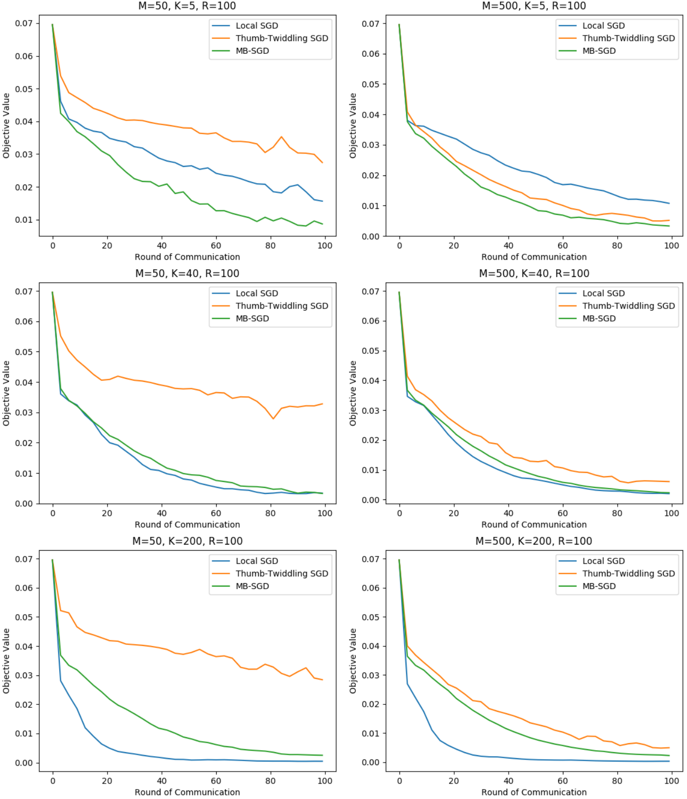
Refer to caption
Figure 6: We constructed a dataset of 50000 points in ℝ25\mathbb{R}^{25} with the iith coordinate of each point distributed independently according to a Gaussian distribution 𝒩⁡(0,10i2)\mathcal{N}(0,\frac{10}{i^{2}}). The labels are generated via ℙ⁡[y=1|x]=σ⁡(min⁡{⟨w1∗,x⟩+b1∗,⟨w2∗,x⟩+b2∗})\mathbb{P}[y=1\,|\,x]=\sigma(\min\{\left\langle w_{1}^{*},\,x\right\rangle+b_{1}^{*},\left\langle w_{2}^{*},\,x\right\rangle+b_{2}^{*}\}) for w1∗,w2∗∼𝒩⁡(0,I25×25)w_{1}^{*},w_{2}^{*}\sim\mathcal{N}(0,I_{25\times 25}) and b1∗,b2∗∼𝒩⁡(0,1)b_{1}^{*},b_{2}^{*}\sim\mathcal{N}(0,1), where σ⁡(a)=1/(1+exp⁡(−a))\sigma(a)=1/(1+\exp(-a)) is the sigmoid function, i.e. the labels correspond to an intersection of two halfspaces with label noise which increases as one approaches the decision boundary. We used each algorithm to train a linear model with a bias term to minimize the logistic loss over the 50000 points, i.e. ff is the logistic loss on one sample and 𝒟\mathcal{D} is the empirical distribution over the 50000 samples. For each MM, KK, and algorithm, we tuned the constant stepsize to minimize the loss after rr rounds of communication individually for each 1≤r≤R1\leq r\leq R. Let x𝖠,r,ηx_{\mathsf{A},r,\eta} denote algorithm 𝖠\mathsf{A}’s iterate after the rrth round of communication when using constant stepsize η\eta. The plotted lines are an approximation of g𝖠​(r)=minη⁡F⁡(x𝖠,r,η)−F⁡(x∗)g_{\mathsf{A}}(r)=\min_{\eta}F(x_{\mathsf{A},r,\eta})-F(x^{*}) for each 𝖠\mathsf{A} where the minimum is calculated using grid search on a log scale.

We will now show that in a certain regime, Local SGD really is inferior (in the worst-case) to Minibatch SGD, and even to Thumb-Twiddling SGD. We show this by constructing a simple, smooth piecewise-quadratic objective in three dimensions on which Local SGD performs poorly. We define this hard instance as F⁡(x)=𝔼z​f​(x,z)F(x)=\mathbb{E}_{z}f(x;z) where

f⁡(x,z)=λ2​(x1−B3)2+H2​(x2−B3)2+H8​((x3−B3)2+(x3−B3)+2)+z​x3f(x;z)=\frac{\lambda}{2}\left(x_{1}-\frac{B}{\sqrt{3}}\right)^{2}+\frac{H}{2}\left(x_{2}-\frac{B}{\sqrt{3}}\right)^{2}+\frac{H}{8}\left(\left(x_{3}-\frac{B}{\sqrt{3}}\right)^{2}+\left(x_{3}-\frac{B}{\sqrt{3}}\right)_{+}^{2}\right)+zx_{3} (99)

and where ℙ[z=σ]=ℙ[z=−σ]=12\P\left[z=\sigma\right]=\P\left[z=-\sigma\right]=\frac{1}{2} and (y)+:=max⁡{y,0}\left(y\right)_{+}:=\max\{y,0\}.

Theorem 7.

For any K≥2K\geq 2, M,R≥1M,R\geq 1, and dimension at least 3, there exists F0∈ℱ0​(H,B)F_{0}\in\mathcal{F}_{0}(H,B) such that the final averaged iterate of Local SGD initialized at 00 with any fixed stepsize will have suboptimality at least

𝔼​F0​(x^)−F0∗≥c⋅(min⁡{(H​σ2​B4)1/3K2/3​R2/3,H​B2}+min⁡{σ​BM​K​R,H​B2})\mathbb{E}F_{0}(\hat{x})-F_{0}^{*}\geq c\cdot\left(\min\left\{\frac{\left(H\sigma^{2}B^{4}\right)^{1/3}}{K^{2/3}R^{2/3}},\,HB^{2}\right\}+\min\left\{\frac{\sigma B}{\sqrt{MKR}},\,HB^{2}\right\}\right)

Similarly, for any λ≤H16\lambda\leq\frac{H}{16}, there exists Fλ∈ℱλ​(H,Δ)F_{\lambda}\in\mathcal{F}_{\lambda}(H,\Delta) such that the final averaged iterate of Local SGD initialized at 00 with any fixed stepsize will have suboptimality at least

𝔼​Fλ​(x^)−Fλ∗≥c⋅(min⁡{H​σ2λ2​K2​R2,Δ}+min⁡{σ2λ​M​K​R,Δ})\mathbb{E}F_{\lambda}(\hat{x})-F_{\lambda}^{*}\geq c\cdot\left(\min\left\{\frac{H\sigma^{2}}{\lambda^{2}K^{2}R^{2}},\,\Delta\right\}+\min\left\{\frac{\sigma^{2}}{\lambda MKR},\Delta\right\}\right)

We defer a detailed proof of Theorem 7 to Appendix B.3. Intuitively, it relies on the fact that for non-quadratic functions, the SGD updates are no longer linear as in Section 4.2.2, and the Local SGD dynamics introduce an additional bias term which does not improve with MM, and scales poorly with K,RK,R. This phenomenon does not seem to be unique to our construction, and should be expected to exist for any “sufficiently non-quadratic” function.

The proof shows specifically that the suboptimality is large unless x3≈B3x_{3}\approx\frac{B}{\sqrt{3}}, but Local SGD introduces a bias which causes x3x_{3} to drift in the negative direction by an amount proportional to the stepsize. On the other hand, optimizing the first term of the objective requires the stepsize to be relatively large. Combining these yields the first term of the lower bound. The second term is classical and holds even for first-order algorithms that compute M​K​RMKR stochastic gradients sequentially (Nemirovsky and Yudin 1983).

In order to compare this lower bound with Theorem 6 and with Minibatch SGD, we again consider the general convex setting with H=B=σ2=1H=B=\sigma^{2}=1. Then, the upper bound reduces to K−13​R−23+(M​K​R)−12K^{-\frac{1}{3}}R^{-\frac{2}{3}}+(MKR)^{-\frac{1}{2}}. Comparing this to Theorem 7, we see that our upper bound is tight up to a factor of K−13K^{-\frac{1}{3}} in the optimization term. Furthermore, comparing the lower bound to the worst-case error of Minibatch SGD (97), we see that Local SGD is indeed worse than Minibatch SGD in the worst case when K≲RK\lesssim\sqrt{R}. Our lower bound is unable to identify the exact cross-over point, but it is some K∗∈[R,R]K^{*}\in[\sqrt{R},R]. For K≤K∗K\leq K^{*}, Minibatch SGD is better than Local SGD in the worst case, for K≥K∗K\geq K^{*}, Local SGD is better. Since the optimization terms of Minibatch SGD and Thumb-Twiddling SGD are identical, this further indicates that Local SGD can even be outperformed by Thumb-Twiddling SGD in the small KK and large MM regime.

For Theorem 7, we constructed a hard instance that is convenient for analysis but is maybe somewhat “artificial.” We also conducted an experiment showing that the same qualitative picture holds also for a more “natural” logistic regression task. In Figure 6, we plot the suboptimality of Local, Minibatch, and Thumb-Twiddling SGD iterates with optimally tuned stepsizes and, as is predicted by Theorem 7, we see Local SGD performing worse than Minibatch in the small K=5K=5 regime, but improving relative to the other algorithms as KK increases to 4040 and then 200200, when Local SGD is far superior to Minibatch. For each fixed KK, increasing MM causes Thumb-Twiddling SGD to improve relative to Minibatch SGD, but does not have a significant effect on Local SGD, which is consistent with the method introducing a bias that depends on KK but not on MM. This highlights that the “problematic regime” for Local SGD is one where there are few iterations per round.

4.3 Local SGD in the Heterogeneous Setting

We now move on to optimization in the intermittent communication setting with heterogeneous data, where the objective has the form F⁡(x)=1M​∑m=1MFm​(x)F(x)=\frac{1}{M}\sum_{m=1}^{M}F_{m}(x) and each of the MM machines has access to a stochastic gradient oracle for its corresponding objective FmF_{m}. Here, we focus on the problem of finding a single consensus solution for FF, which achieves a low value on all of the local objectives F1,…,FMF_{1},\dots,F_{M} on average (Bertsekas and Tsitsiklis 1989; Boyd et al. 2011). Because each machine only has access to a single component of the objective, the heterogeneous is substantially harder than the previously considered homogeneous case.

Like in the homogeneous setting, a number of recent papers have analyzed the convergence properties of Local SGD in the heterogeneous data setting (Wang and Joshi 2018; Karimireddy et al. 2019; Khaled et al. 2020; Koloskova et al. 2020). Also as in the homogeneous setting, we will show that none of these Local SGD guarantees show improvement over the baseline of Minibatch SGD, even without acceleration, and in many regimes their guarantees are much worse. This again raises the question of whether this a weakness of the analysis or the Local SGD method itself. Can the bounds be improved to show that Local SGD is actually better than Minibatch SGD in certain regimes, or is Local SGD always worse?

Recall that in the homogeneous setting, prior analysis had not been able to show that Local SGD improves over Minibatch SGD yet the combination of Theorem 6 and Theorem 7 showed that Local SGD is better than Minibatch SGD in some regimes and worse in others. Specifically, when communication was relatively infrequent Local SGD improves over Minibatch SGD.

How does this situation play out in the more challenging, and perhaps more interesting, heterogeneous setting? In several discussions following the publication of Woodworth et al. 2020b, people had suggested that the more difficult heterogeneous setting is where we should expect Local SGD to really shine, and that Minibatch SGD is too naïve. So, how does heterogeneity affect Local SGD, Minibatch SGD, and the comparison between them? Is Local SGD better than Minibatch SGD when communication is rare as in the homogeneous case? Does the difficulty introduced by heterogeneity perhaps necessitate the more sophisticated Local SGD approach, as some have suggested?

In recent work, Karimireddy et al. 2019 showed heterogeneity can be problematic for Local SGD, proving a lower bound that indicates some degradation as degree of heterogeneity increases. As we will discuss, this lower bound implies that Local SGD is strictly worse than Minibatch SGD when the level of heterogeneity is very large, but it is not clear whether or not Local SGD can improve over Minibatch SGD for slightly or moderately heterogeneous objectives.

Boundedly Heterogeneous Objectives

In addition to the usual assumptions of smoothness and convexity/strong convexity, we will introduce a new parameter that captures the extent to which the local objectives disagree about the minimizer. In particular, we will say that a heterogeneous objective F⁡(x)=1M​∑m=1MFm​(x)F(x)=\frac{1}{M}\sum_{m=1}^{M}F_{m}(x) is ζ∗2\zeta_{*}^{2}-heterogeneous if, for some x∗∈arg​minx⁡F​(x)x^{*}\in\argmin_{x}F(x)

1M​∑m=1M‖∇Fm​(x∗)‖2≤ζ∗2\frac{1}{M}\sum_{m=1}^{M}\left\|\nabla F_{m}(x^{*})\right\|^{2}\leq\zeta_{*}^{2} (100)

Since ∇F​(x∗)=0\nabla F(x^{*})=0, this can be thought of as measuring the variance of the gradient at x∗x^{*} when selecting a random component. If the objective is 00-heterogeneous, then all of the objectives share a minimizer, but we note that it does not imply that all the local objectives are the same, since (100) is only a statement about the gradients at x∗x^{*}. This assumption of ζ∗2\zeta_{*}^{2}-heterogeneity is common in the Local SGD literature (Karimireddy et al. 2019; Khaled et al. 2020; Koloskova et al. 2020) and it is used to prove most of the convergence guarantees for Local SGD that we are aware of. Nevertheless, in the consensus optimization literature, it is common to analyze distributed algorithms with no such bound on the heterogeneity, and it is certainly still possible to minimize FF without this assumption (Boyd et al. 2011; Nedic and Ozdaglar 2009; Nedic et al. 2010; Ram et al. 2010).

We define the function class ℱ0​(H,B,M,ζ∗2)\mathcal{F}_{0}(H,B,M,\zeta_{*}^{2}) as the class of ζ∗2\zeta_{*}^{2}-heterogeneous objectives of the form F⁡(x)=1M​∑m=1MFm​(x)F(x)=\frac{1}{M}\sum_{m=1}^{M}F_{m}(x) where FmF_{m} is HH-smooth for all mm, and F∈ℱ0​(H,B)F\in\mathcal{F}_{0}(H,B). Similarly, we define ℱλ​(H,Δ,M,ζ∗2)\mathcal{F}_{\lambda}(H,\Delta,M,\zeta_{*}^{2}) as the class of ζ∗2\zeta_{*}^{2}-heterogeneous objectives of the form F⁡(x)=1M​∑m=1MFm​(x)F(x)=\frac{1}{M}\sum_{m=1}^{M}F_{m}(x) where FmF_{m} is HH-smooth for all mm, and F∈ℱλ​(H,Δ)F\in\mathcal{F}_{\lambda}(H,\Delta).

4.3.1 Minibatch SGD in the Heterogeneous Setting

To begin, we analyze the worst-case error of our baseline Minibatch SGD and Minibatch AC-SA (Lan 2012; Ghadimi and Lan 2013a) (see Algorithm 1) in the heterogeneous setting. A simple but important observation is that the minibatch gradients used by these algorithms are unbiased estimates of ∇F\nabla F despite the heterogeneity of the objective:

𝔼⁡[1M​K​∑m=1M∑k=1Kg⁡(xr,zr,km)]=1M​∑m=1M∇Fm​(xr)=∇F​(xr)\mathbb{E}\left[\frac{1}{MK}\sum_{m=1}^{M}\sum_{k=1}^{K}g(x_{r};z_{r,k}^{m})\right]=\frac{1}{M}\sum_{m=1}^{M}\nabla F_{m}(x_{r})=\nabla F(x_{r}) (101)

Since the minibatch stochastic gradients are unbiased estimates of ∇F\nabla F, we can simply appeal to the standard analysis for (accelerated) SGD. To do so, we calculate the variance of these estimates:

𝔼​‖1M​K​∑m=1M∑k=1Kg⁡(xr,zr,km)−∇F​(xr)‖2\displaystyle\mathbb{E}\left\|\frac{1}{MK}\sum_{m=1}^{M}\sum_{k=1}^{K}g(x_{r};z_{r,k}^{m})-\nabla F(x_{r})\right\|^{2} =1M2​K2​∑m=1M∑k=1K𝔼​‖g⁡(xr,zr,km)−∇Fm​(xr)‖2≤σ2M​K\displaystyle=\frac{1}{M^{2}K^{2}}\sum_{m=1}^{M}\sum_{k=1}^{K}\mathbb{E}\left\|g(x_{r};z_{r,k}^{m})-\nabla F_{m}(x_{r})\right\|^{2}\leq\frac{\sigma^{2}}{MK} (102)

So, the variance is always reduced by M​KMK and, importantly, it is not affected by the level of heterogeneity ζ∗\zeta_{*}. Plugging this calculation into the analysis of SGD and Accelerated SGD (Nemirovsky and Yudin 1983; Lan 2012) yields:

Theorem 8.

For any F0∈ℱ0​(H,B,M,ζ∗2)F_{0}\in\mathcal{F}_{0}(H,B,M,\zeta_{*}^{2}) and any Fλ∈ℱλ​(H,Δ,M,ζ∗2)F_{\lambda}\in\mathcal{F}_{\lambda}(H,\Delta,M,\zeta_{*}^{2}), the output of Minibatch SGD guarantees

𝔼​F0​(x^)−F0∗\displaystyle\mathbb{E}F_{0}(\hat{x})-F_{0}^{*} ≤c⋅(H​B2R+σ​BM​K​R)\displaystyle\leq c\cdot\left(\frac{HB^{2}}{R}+\frac{\sigma B}{\sqrt{MKR}}\right)
𝔼​Fλ​(x^)−Fλ∗\displaystyle\mathbb{E}F_{\lambda}(\hat{x})-F_{\lambda}^{*} ≤c⋅(H​Δλ​exp⁡(−λ​R2​H)+σ2λ​M​K​R)\displaystyle\leq c\cdot\left(\frac{H\Delta}{\lambda}\exp\left(-\frac{\lambda R}{2H}\right)+\frac{\sigma^{2}}{\lambda MKR}\right)

and Minibatch AC-SA guarantees

𝔼​F0​(x^)−F0∗\displaystyle\mathbb{E}F_{0}(\hat{x})-F_{0}^{*} ≤c⋅(H​B2R2+σ​BM​K​R)\displaystyle\leq c\cdot\left(\frac{HB^{2}}{R^{2}}+\frac{\sigma B}{\sqrt{MKR}}\right)
𝔼​Fλ​(x^)−Fλ∗\displaystyle\mathbb{E}F_{\lambda}(\hat{x})-F_{\lambda}^{*} ≤c⋅(Δ​exp⁡(−λ​Rc3​H)+σ2λ​M​K​R)\displaystyle\leq c\cdot\left(\Delta\exp\left(-\frac{\sqrt{\lambda}R}{c_{3}\sqrt{H}}\right)+\frac{\sigma^{2}}{\lambda MKR}\right)

The theorem follows immediately from the observation about the unbiaseness and variance of the stochastic gradients above, and previously established convergence rates for SGD (Nemirovsky and Yudin 1983; Stich 2019) and AC-SA (Lan 2012; Ghadimi and Lan 2013a). The most important feature of these guarantees is that they are completely independent of ζ∗2\zeta_{*}^{2} because of the use of minibatch stochastic gradients. In the following sections, we will see how Local SGD compares.

4.3.2 Prior Analysis of Local SGD in the Heterogeneous Setting

Algorithm Suboptimality Bound
Minibatch SGD: Theorem 8 H​B2R+σ​BM​K​R\frac{HB^{2}}{R}+\frac{\sigma B}{\sqrt{MKR}}
Local SGD: Koloskova et al. 2020 H​B2R+σ​BM​K​R+(H​ζ∗2​B4)1/3R2/3+(H​σ2​B4)1/3K1/3​R2/3\frac{HB^{2}}{R}+\frac{\sigma B}{\sqrt{MKR}}+\frac{(H\zeta_{*}^{2}B^{4})^{1/3}}{R^{2/3}}+\frac{(H\sigma^{2}B^{4})^{1/3}}{K^{1/3}R^{2/3}}
Local SGD: Khaled et al. 2020 H​B2R+B​σ2+ζ∗2M​K​R+(H⁡(σ2+ζ∗2)​B4)1/3R2/3\frac{HB^{2}}{R}+\frac{B\sqrt{\sigma^{2}+\zeta_{*}^{2}}}{\sqrt{MKR}}+\frac{(H(\sigma^{2}+\zeta_{*}^{2})B^{4})^{1/3}}{R^{2/3}}
SCAFFOLD: Karimireddy et al. 2019 H​B2R+σ​BM​K​R+σ2H​K​R\frac{HB^{2}}{R}+\frac{\sigma B}{\sqrt{MKR}}+\frac{\sigma^{2}}{HKR}
Local SGD: Theorem 10 H​B2K​R+σ​BM​K​R+(H​ζ¯2​B4)1/3R2/3+(H​σ2​B4)1/3K1/3​R2/3\frac{HB^{2}}{KR}+\frac{\sigma B}{\sqrt{MKR}}+\frac{(H\bar{\zeta}^{2}B^{4})^{1/3}}{R^{2/3}}+\frac{(H\sigma^{2}B^{4})^{1/3}}{K^{1/3}R^{2/3}}
Local SGD Lower Bound: Theorem 9 min⁡{H​B2R,(H​ζ∗2​B4)1/3R2/3}+σ​BM​K​R+(H​σ2​B4)1/3K2/3​R2/3\min\left\{\frac{HB^{2}}{R},\,\frac{(H\zeta_{*}^{2}B^{4})^{1/3}}{R^{2/3}}\right\}+\frac{\sigma B}{\sqrt{MKR}}+\frac{(H\sigma^{2}B^{4})^{1/3}}{K^{2/3}R^{2/3}}
Table 2: Guarantees for objectives in ℱ0​(H,B,M,ζ∗2)\mathcal{F}_{0}(H,B,M,\zeta_{*}^{2}). See the discussion around Theorem 10 for the definition of ζ¯\bar{\zeta}.
Algorithm Suboptimality Bound
Minibatch SGD: Theorem 8 H​Δλ​exp⁡(−λ​RH)+σ∗2λ​M​K​R\frac{H\Delta}{\lambda}\exp\left(\frac{-\lambda R}{H}\right)+\frac{\sigma_{*}^{2}}{\lambda MKR}
Local SGD: Koloskova et al. 2020 Δ​exp⁡(−λ​RH)+σ∗2λ​M​K​R+H​ζ∗2λ2​R2+H​σ∗2λ2​K​R2\Delta\exp\left(\frac{-\lambda R}{H}\right)+\frac{\sigma_{*}^{2}}{\lambda MKR}+\frac{H\zeta_{*}^{2}}{\lambda^{2}R^{2}}+\frac{H\sigma_{*}^{2}}{\lambda^{2}KR^{2}}
SCAFFOLD: Karimireddy et al. 2019 (Δ+λ​σ2H2​K)​exp⁡(−λ​RH)+σ2λ​M​K​R\left(\Delta+\frac{\lambda\sigma^{2}}{H^{2}K}\right)\exp\left(\frac{-\lambda R}{H}\right)+\frac{\sigma^{2}}{\lambda MKR}
Local SGD: Theorem 10 H​Δλ​exp⁡(−c′​λ​K​RH)+σ2λ​M​K​R+H​ζ¯2λ2​R2+H​σ2λ2​K​R2\frac{H\Delta}{\lambda}\exp\left(-\frac{c^{\prime}\lambda KR}{H}\right)+\frac{\sigma^{2}}{\lambda MKR}+\frac{H\bar{\zeta}^{2}}{\lambda^{2}R^{2}}+\frac{H\sigma^{2}}{\lambda^{2}KR^{2}}
Local SGD Lower Bound: Theorem 9 min⁡{Δ​exp⁡(−λ​RH),H​ζ∗2λ2​R2}+σ2λ​M​K​R+min⁡{Δ,H​σ2λ2​K2​R2}\min\left\{\Delta\exp\left(\frac{-\lambda R}{H}\right),\,\frac{H\zeta_{*}^{2}}{\lambda^{2}R^{2}}\right\}+\frac{\sigma^{2}}{\lambda MKR}+\min\left\{\Delta,\,\frac{H\sigma^{2}}{\lambda^{2}K^{2}R^{2}}\right\}
Table 3: Guarantees for objectives in ℱλ​(H,Δ,M,ζ∗2)\mathcal{F}_{\lambda}(H,\Delta,M,\zeta_{*}^{2}), with some log factors omitted. See the discussion around Theorem 10 for the definition of ζ¯\bar{\zeta}.

Recently, Khaled et al. 2020 and Koloskova et al. 2020 analyzed Local SGD in the heterogeneous and convex setting, and Koloskova et al. 2020 did also in the strongly convex setting. Their guarantees are summarized in Table 2 and Table 3. Also included are guarantees for SCAFFOLD77 7 Karimireddy et al. 2019 analyze SCAFFOLD in the Federated Learning setting where only a random subset of S≤MS\leq M of the machines are available in each round. Here, we present the analysis as it applies to our setting where S=MS=M., a related method for heterogeneous distributed optimization (Karimireddy et al. 2019).

Upon inspection, Koloskova et al. 2020’s guarantee is slightly better than Khaled et al. 2020, but even this guarantee is (up to logarithmic terms) the sum of the Minibatch SGD bound plus additional terms, and is thus always worse in every regime. The question is whether this just reflects a weakness of their analysis, or a true weakness of the Local SGD algorithm?

Indeed, Theorem 6 shows that a tighter upper bound for Local SGD is possible in the homogeneous case, and this rate is better than Koloskova et al. 2020’s when ζ∗2=0\zeta_{*}^{2}=088 8 Although, we remind the reader that ζ∗2=0\zeta_{*}^{2}=0 does not imply that the problem is homogeneous.. Can we generalize Theorem 6 to the heterogeneous case and show improvement over Minibatch SGD?

Optimistically, we might hope that Koloskova et al. 2020’s (ζ∗/R)2/3(\zeta_{*}/R)^{2/3} term, in particular, could be improved. Unfortunately, it is already known that some dependence on ζ∗\zeta_{*} is necessary, as Karimireddy et al. 2019 shows a lower bound of ζ∗2/(λ​R2)\zeta_{*}^{2}/(\lambda R^{2}) in the strongly convex case, which suggests a lower bound of ζ∗​B/R\zeta_{*}B/R in the convex case. But perhaps the Koloskova et al. 2020 analysis can be improved to match this bound?

If the ζ∗​B/R\zeta_{*}B/R dependence suggested by Karimireddy et al. 2019’s lower bound were possible, it would be lower-order than H​B2/RHB^{2}/R for ζ∗<H​B\zeta_{*}<HB, and we would see no slow down until the level of heterogeneity is fairly large. In particular, since the components FmF_{m} are HH-smooth, adding the assumption that the local objectives FmF_{m} each have a minimizer of norm at most O⁡(B)O(B) would be enough to bound ζ∗≤O⁡(H​B)\zeta_{*}\leq O(HB). In this case, the dependence on the level of heterogeneity would be fairly mild, and could be ignored under reasonable circumstances. On the other hand, if the (ζ∗/R)2/3(\zeta_{*}/R)^{2/3} term from Koloskova et al. 2020 cannot be improved, then we see a slowdown as soon as ζ∗=Ω⁡(H​B/R)\zeta_{*}=\Omega(HB/R), which corresponds to a quite low level of heterogeneity! So, what is the correct rate?

4.3.3 Upper and Lower Bounds for Local SGD in the Heterogeneous Setting

We now show that the poor dependence on ζ∗\zeta_{*} from Koloskova et al. 2020’s analysis cannot be improved. Consequently, for sufficiently heterogeneous data, Local SGD is strictly worse than Minibatch SGD, regardless of the frequency of communication, unless the level of heterogeneity is very small.

Theorem 9.

For K≥2K\geq 2 and any dimension at least 4, there exists an objective F0∈ℱ0​(H,B,M,ζ∗2)F_{0}\in\mathcal{F}_{0}(H,B,M,\zeta_{*}^{2}) and for any λ≤H16\lambda\leq\frac{H}{16}, there exists Fλ∈ℱλ​(H,Δ,M,ζ∗2)F_{\lambda}\in\mathcal{F}_{\lambda}(H,\Delta,M,\zeta_{*}^{2}) such that the final averaged iterate of Local SGD initialized at zero and using any fixed stepsize η\eta will have suboptimality at least

𝔼​F0​(x^)−F0∗\displaystyle\mathbb{E}F_{0}(\hat{x})-F_{0}^{*} ≥c⋅(min⁡{H​B2R,(H​ζ∗2​B4)1/3R2/3}+(H​σ2​B4)1/3K2/3​R2/3+σ​BM​K​R)\displaystyle\geq c\cdot\left(\min\left\{\frac{HB^{2}}{R},\,\frac{\left(H\zeta_{*}^{2}B^{4}\right)^{1/3}}{R^{2/3}}\right\}+\frac{\left(H\sigma^{2}B^{4}\right)^{1/3}}{K^{2/3}R^{2/3}}+\frac{\sigma B}{\sqrt{MKR}}\right)
𝔼​Fλ​(x^)−Fλ∗\displaystyle\mathbb{E}F_{\lambda}(\hat{x})-F_{\lambda}^{*} ≥c⋅(min⁡{Δ​exp⁡(−c′​λ​RH),H​ζ∗2λ2​R2}+min⁡{Δ,H​σ2λ2​K2​R2}+σ2λ​M​K​R)\displaystyle\geq c\cdot\left(\min\left\{\Delta\exp\left(-\frac{c^{\prime}\lambda R}{H}\right),\,\frac{H\zeta_{*}^{2}}{\lambda^{2}R^{2}}\right\}+\min\left\{\Delta,\,\frac{H\sigma^{2}}{\lambda^{2}K^{2}R^{2}}\right\}+\frac{\sigma^{2}}{\lambda MKR}\right)

This is proven in Appendix B.4 using a similar approach as Theorem 7, and it is conceptually similar to the lower bounds for heterogeneous objectives of Karimireddy et al. 2019. Koloskova et al. 2020 also prove a lower bound, but specifically for 1-strongly convex objectives, which obscures the important role of the strong convexity parameter.

In the convex case, this lower bound closely resembles the upper bound of Koloskova et al. 2020. Focusing on the case H=B=σ2=1H=B=\sigma^{2}=1 to emphasize the role of ζ∗2\zeta_{*}^{2}, the only gaps are between (i) a term 1/(K1/3​R2/3)1/(K^{1/3}R^{2/3}) vs 1/(K2/3​R2/3)1/(K^{2/3}R^{2/3})—a gap which also exists in the homogeneous case (see Theorem 6 and Theorem 7)—and (ii) another term 1/R+(ζ∗/R)2/31/R+(\zeta_{*}/R)^{2/3} vs min⁡{1/R,(ζ∗/R)2/3}\min\{1/R,\ (\zeta_{*}/R)^{2/3}\}.

For ζ∗2≥1/R⇒(ζ∗/R)2/3≥1/R\zeta_{*}^{2}\geq 1/R\Rightarrow(\zeta_{*}/R)^{2/3}\geq 1/R, the lower bound shows that Local SGD has error at least 1/R+1/M​K​R1/R+1/\sqrt{MKR} and thus performs strictly worse than Minibatch, regardless of KK. This is quite surprising—Local SGD is often suggested as an improvement over Minibatch SGD for the heterogeneous setting, yet we see that even a small degree of heterogeneity can make it much worse. Furthermore, increasing the duration of each round, KK, is often thought of as more beneficial for Local SGD than Minibatch SGD, but the lower bound indicates it does little to help Local SGD in the heterogeneous setting.

Similarly, in the strongly convex case, the lower bound from Theorem 9 nearly matches the upper bound of Koloskova et al. 2020. Focusing on the case H=B=σ=1H=B=\sigma=1 in order to emphasize the role of ζ∗\zeta_{*}, the only differences are between (i) a term 1/(K​R2)1/(KR^{2}) versus 1/(K2​R2)1/(K^{2}R^{2})—a gap which also exists in the homogeneous case (see Theorem 6 and Theorem 7)—and (ii) between exp⁡(−λ​R)+ζ∗2/(λ2​R2)\exp(-\lambda R)+\zeta_{*}^{2}/(\lambda^{2}R^{2}) and min⁡{exp⁡(−λ​R),ζ∗2/(λ2​R2)}\min\left\{\exp(-\lambda R),\,\zeta_{*}^{2}/(\lambda^{2}R^{2})\right\}. The latter gap is more substantial than the convex case, but nevertheless indicates that the ζ∗2/(λ2​R2)\zeta_{*}^{2}/(\lambda^{2}R^{2}) rate cannot be improved until the number of rounds of communication is at least the condition number or ζ∗2\zeta_{*}^{2} is very small.

Thus, Theorem 9 indicates that it is not possible to radically improve over the Koloskova et al. 2020 analysis, and thus over Minibatch SGD for even moderate heterogeneity, without stronger assumptions. In order to obtain an improvement over Minibatch SGD in a heterogeneous setting, at least with very low heterogeneity, we introduce a stronger version of the heterogeneity measure ζ∗\zeta_{*} which bounds the difference between the local objectives’ gradients everywhere, not just at x∗x^{*}:

supx1M​∑m=1M‖∇Fm​(x)−∇F​(x)‖2≤ζ¯2\sup_{x}\frac{1}{M}\sum_{m=1}^{M}\left\|\nabla F_{m}(x)-\nabla F(x)\right\|^{2}\leq\bar{\zeta}^{2} (103)

This quantity precisely captures homogeneity since ζ¯2=0\bar{\zeta}^{2}=0 if and only if Fm=FF_{m}=F (up to an irrelevant additive constant). In terms of ζ¯2\bar{\zeta}^{2}, we are able to analyze Local SGD and see a smooth transition from the heterogeneous (ζ¯2\bar{\zeta}^{2} large) to homogeneous (ζ¯2=0\bar{\zeta}^{2}=0) setting.

Theorem 10.

For any F0∈ℱ0​(H,B,M,ζ∗2)F_{0}\in\mathcal{F}_{0}(H,B,M,\zeta_{*}^{2}) and any Fλ∈ℱλ​(H,Δ,M,ζ∗2)F_{\lambda}\in\mathcal{F}_{\lambda}(H,\Delta,M,\zeta_{*}^{2}) with the additional property that supx1M​∑m=1M‖∇Fm​(x)−∇F​(x)‖2≤ζ¯2\sup_{x}\frac{1}{M}\sum_{m=1}^{M}\left\|\nabla F_{m}(x)-\nabla F(x)\right\|^{2}\leq\bar{\zeta}^{2}, Local SGD guarantees

𝔼​F0​(x^)−F0∗\displaystyle\mathbb{E}F_{0}(\hat{x})-F_{0}^{*} ≤c⋅(H​B2K​R+(H​ζ¯2​B4)1/3R2/3+(H​σ2​B4)1/3K1/3​R2/3+σ​BM​K​R),\displaystyle\leq c\cdot\left(\frac{HB^{2}}{KR}+\frac{\left(H\bar{\zeta}^{2}B^{4}\right)^{1/3}}{R^{2/3}}+\frac{\left(H\sigma^{2}B^{4}\right)^{1/3}}{K^{1/3}R^{2/3}}+\frac{\sigma B}{\sqrt{MKR}}\right),
𝔼​Fλ​(x^)−Fλ∗\displaystyle\mathbb{E}F_{\lambda}(\hat{x})-F_{\lambda}^{*} ≤c⋅(H​Δλ​exp⁡(−c′​λ​K​RH)+(H​ζ¯2λ2​R2+H​σ2λ2​K​R2)​log⁡(e+λ​K​RH)+σ2λ​M​K​R).\displaystyle\leq c\cdot\left(\frac{H\Delta}{\lambda}\exp\left(-\frac{c^{\prime}\lambda KR}{H}\right)+\left(\frac{H\bar{\zeta}^{2}}{\lambda^{2}R^{2}}+\frac{H\sigma^{2}}{\lambda^{2}KR^{2}}\right)\log\left(e+\frac{\lambda KR}{H}\right)+\frac{\sigma^{2}}{\lambda MKR}\right).

We prove this in Appendix B.5. This is the first analysis of Local SGD, or any other method for heterogeneous distributed optimization, which shows any improvement over Minibatch SGD in any heterogeneous regime. When ζ¯=0\bar{\zeta}=0, Theorem 10 reduces to the homogeneous analysis of Local SGD given by Theorem 6, which already showed that in that case, we see improvement when K≳RK\gtrsim R. Theorem 10 degrades smoothly when ζ¯\bar{\zeta} increases, and shows improvement for Local SGD over Minibatch SGD also when ζ¯2≲1/R\bar{\zeta}^{2}\lesssim 1/R in the convex case, i.e. with low, yet positive, heterogeneity. It is yet unclear whether this rate of convergence can be ensured in terms of ζ∗2\zeta_{*}^{2} rather than ζ¯2\bar{\zeta}^{2}.

Experimental evidence

Finally, while Theorem 9 proves that Local SGD is worse than Minibatch SGD unless ζ∗\zeta_{*} is very small in the worst case, one might hope that for “normal” heterogeneous problems, Local SGD might perform better than its worst case error suggests. However, a simple binary logistic regression experiment on MNIST indicates that this behavior likely extends significantly beyond the worst case. The results, depicted in Figure 7, show that Local SGD performs worse than Minibatch SGD unless both ζ∗\zeta_{*} is very small and KK is large. Finally, we also observe that Minibatch SGD’s performance is essentially unaffected by ζ∗\zeta_{*} empirically as predicted by theory.

Refer to caption
Refer to caption
Figure 7: Binary logistic regression between even vs odd digits of MNIST. Twenty-five “tasks” were constructed, one for each combination of ii vs jj for even ii and odd jj. For p∈{0,20,40,60,80,100}p\in\{0,20,40,60,80,100\}, we assigned to each of M=25M=25 machines p%p\% data from task mm, and (100−p)%(100-p)\% data from a mixture of all tasks. For several choices of RR and KK, we plot the error (averaged over four runs) versus the value of ζ∗2\zeta_{*}^{2} resulting from each choice of pp. For both algorithms, we used the best fixed stepsize for each choice of KK, RR, and ζ∗\zeta_{*} individually. Complete details are provided in Appendix B.6.

4.4 Conclusion

In the homogeneous setting we showed that: (1) Local SGD attains very low error for quadratic objectives, and strictly dominates the baselines of Single-Machine SGD and Minibatch SGD; (2) for general objectives, Local SGD is always at least as good as Single-Machine SGD, and it is strictly better than Minibatch SGD when communication is relatively infrequent (K≳RK\gtrsim R); and (3) Local SGD is strictly worse than Minibatch SGD when communication is relatively frequent (K≲RK\lesssim\sqrt{R}), and it can even be worse than Thumb-Twiddling SGD.

In the heterogeneous setting, Local SGD compares relatively less favorably against Minibatch SGD. For ζ∗2\zeta_{*}^{2}-heterogeneous functions, no existing analysis shows any improvement over Minibatch SGD in any regime, and our lower bound shows that no such improvement is possible as soon as ζ∗2≳1/R\zeta_{*}^{2}\gtrsim 1/R. On the other hand, when the heterogeneity is bounded everywhere by ζ¯2\bar{\zeta}^{2}, then we show that Local SGD can improve over Minibatch SGD, at least when ζ¯2≲1/R\bar{\zeta}^{2}\lesssim 1/R.

To better understand the relationship between Minibatch SGD and Local SGD, and for thinking about how to improve over them, it is useful to consider a unified algorithm that interpolates between them. This involves taking SGD steps locally with one stepsize, and then when the machines communicate, they take a step in the resulting direction with a second, different stepsize. Such a dual-stepsize approach was already presented and analyzed as FedAvg by Karimireddy et al. 2019. We will refer to these two stepsizes as “inner” and “outer” stepsizes, respectively, and consider

xr,km\displaystyle x_{r,k}^{m} =xr,k−1m−ηinner​g​(xr,k−1m,zr,k−1m)\displaystyle=x_{r,k-1}^{m}-\eta_{\textrm{inner}}g(x_{r,k-1}^{m};z_{r,k-1}^{m}) ∀m∈[M],k∈[K]\displaystyle\quad\forall_{m\in[M],k\in[K]} (104)
xr+1,0m\displaystyle x_{r+1,0}^{m} =xr,0m−ηouter​1M​∑n=1M∑k=1Kg⁡(xr,k−1m,zr,k−1m)\displaystyle=x_{r,0}^{m}-\eta_{\textrm{outer}}\frac{1}{M}\sum_{n=1}^{M}\sum_{k=1}^{K}g(x_{r,k-1}^{m};z_{r,k-1}^{m}) ∀m∈[M],r∈[R]\displaystyle\quad\forall_{m\in[M],r\in[R]}

Choosing ηinner=0\eta_{\textrm{inner}}=0, this is equivalent to Minibatch SGD with stepsize ηouter\eta_{\textrm{outer}}, and choosing ηinner=ηouter\eta_{\textrm{inner}}=\eta_{\textrm{outer}} recovers Local SGD. Therefore, when the stepsizes are chosen optimally, this algorithm is always at least as good as both Minibatch and Local SGD. Therefore, using the inner-outer algorithm (104) with optimal stepsizes guarantees for F0∈ℱ0​(H,B,M,ζ∗2)F_{0}\in\mathcal{F}_{0}(H,B,M,\zeta_{*}^{2})

𝔼​F0​(x^)−F0∗≤c⋅min⁡{H​B2R+σ​BM​K​R,H​B2K​R+(H​ζ¯2​B4)1/3R2/3+(H​σ2​B4)1/3K1/3​R2/3+σ∗​BM​K​R}\mathbb{E}F_{0}(\hat{x})-F_{0}^{*}\leq c\cdot\min\bigg\{\frac{HB^{2}}{R}+\frac{\sigma B}{\sqrt{MKR}},\frac{HB^{2}}{KR}+\frac{\left(H\bar{\zeta}^{2}B^{4}\right)^{1/3}}{R^{2/3}}+\frac{\left(H\sigma^{2}B^{4}\right)^{1/3}}{K^{1/3}R^{2/3}}+\frac{\sigma_{*}B}{\sqrt{MKR}}\;\bigg\} (105)

where the first option in the min\min is obtained by choosing ηinner=0\eta_{\textrm{inner}}=0 and the second by choosing ηinner=ηouter\eta_{\textrm{inner}}=\eta_{\textrm{outer}}. We can also get a similar minimum of the Minibatch SGD and Local SGD rates in the strongly convex case and also in the homogeneous setting.

5 The Intermittent Communication Setting

In the intermittent communication setting, MM parallel workers are used to optimize a single objective over the course of RR rounds. During each round, each machine sequentially and locally computes KK independent unbiased stochastic gradients of the global objective, and then all the machines communicate with each other. This captures, for example, the natural setting where multiple parallel workers are available, and computation on each worker is much faster than communication between workers. It includes applications ranging from optimization using multiple cores or GPUs, to using a cluster of servers, to Federated Learning where workers are edge devices.

As a concrete example, Goyal et al. 2017 were able to train a large ResNet-50 neural network on Imagenet in under an hour using SGD with very large minibatches, which was implemented in exactly the intermittent communication setting. Specifically, they used M=256M=256 GPUs in parallel, computed KK stochastic gradients per communication between the GPUs, and performed roughly R=10000R=10000 updates/communications. This is, of course, just one example, but it is indicative of many practical uses of distributed optimization for training large machine learning models.

The theoretical properties of optimization algorithms in the intermittent communication setting have been widely studied for over a decade, with many approaches proposed and analyzed (Zinkevich et al. 2010; Cotter et al. 2011; Dekel et al. 2012; Zhang et al. 2013a; Zhang et al. 2013c; Shamir and Srebro 2014), and obtaining new methods and improved analysis is still a very active area of research (Wang et al. 2017; Stich 2018; Wang and Joshi 2018; Khaled et al. 2019; Haddadpour et al. 2019a; Woodworth et al. 2020b). However, despite these efforts, we do not yet know which methods are optimal, what the minimax complexity is, and what methodological or analytical improvements might allow us to make further progress.

A key issue in the existing literature is that known lower bounds for the intermittent communication setting depend only on the product K​RKR (i.e. the total number of gradients computed on each machine over the course of optimization), and not on the number of rounds, RR, and the number of gradients per round, KK, separately. Thus, existing results cannot rule out the possibility that the optimal rate for fixed T=K​RT=KR can be achieved using only a single round of communication (R=1R=1), since they do not distinguish between methods that communicate very frequently (R=TR=T, K=1K=1) and methods that communicate just once (R=1R=1, K=TK=T). The possibility that the optimal rate is achievable with R=1R=1 was suggested by Zhang et al. 2013c, and indeed we showed in Section 4.2 that in the special case of quadratic objectives, Local SGD and Local AC-SA perform just as well with a single communication as they do with many rounds of communication. While it seems unlikely that a single round of communication suffices in the general case, none of our existing lower bounds are able to answer this extremely basic question.

In Section 5.1, we resolve (up to a logarithmic factor) the minimax complexity of smooth, convex stochastic optimization in the homogeneous intermittent communication setting and we show that, generally speaking, a single round of communication does not suffice to achieve the min-max optimal rate. In Section 5.1.1, we prove lower bounds on the optimal rate of convergence with matching upper bounds for convex and strongly convex objectives, and in Section 5.1.3, we prove matching upper and lower bounds on the optimal rate for finding approximate stationary points of non-convex objectives.

Interestingly, in all of these cases we show that the combination of two extremely simple and naïve methods are optimal. In the convex setting, the methods are based on an accelerated SGD variant AC-SA (Lan 2012). Specifically, we show that the better of the following methods is optimal: Minibatch AC-SA which executes RR steps of AC-SA using minibatch gradients of size M​KMK, and Single-Machine AC-SA which executes K​RKR steps of AC-SA on just one of the machines, completely ignoring the other M−1M-1. Similarly, in the non-convex setting, the better of Minibatch SGD and Single-Machine SGD are optimal.

These methods might appear suboptimal: the Minibatch methods only perform one update per round of communication, and the Single-Machine methods only use one of the available workers! This perceived inefficiency has prompted many attempts at developing improved methods which take multiple steps on each machine locally in parallel including, in particular, numerous analyses of Local SGD (Zinkevich et al. 2010; Dekel et al. 2012; Stich 2018; Haddadpour et al. 2019a; Khaled et al. 2019; Woodworth et al. 2020b; Woodworth et al. 2020a), which we already discussed in Section 4. Nevertheless, we establish that one or the other is optimal in every regime, so more sophisticated methods cannot yield improved guarantees for arbitrary smooth objectives. Our results therefore highlight an apparent dichotomy between exploiting the available parallelism but not the local computation (Minibatch) and exploiting the local computation but not the parallelism (Single-Machine).

In addition to the homogeneous setting, in Section 5.2, we also study the heterogeneous setting. Here, we also prove matching upper and lower bounds for convex and strongly convex objectives which establishes that Minibatch AC-SA is minimax optimal.

Our lower bounds apply quite broadly, including to the settings covered by the bulk of the existing work on stochastic first-order optimization in the intermittent communication setting. However, like many lower bounds, we should not interpret them to mean that progress is impossible, and that we are stuck with naïve algorithms like Minibatch SGD. Instead, these results indicate that we need to modify our assumptions in order to develop better methods. In Section 6 we explore several additional assumptions that allow—or might plausibly allow—for circumventing the lower bounds in various ways. These include when the third derivative of the objective is bounded (as in recent work by Yuan and Ma 2020), when the objective has a certain statistical learning-like structure, or when the algorithm has access to a more powerful oracle.

Setting Function Class Minimax Error
Homogeneous ℱ0​(H,B)\mathcal{F}_{0}(H,B) H​B2K2​R2+σ​BM​K​R+min⁡{H​B2R2,σ​BK​R}\frac{HB^{2}}{K^{2}R^{2}}+\frac{\sigma B}{\sqrt{MKR}}+\min\left\{\frac{HB^{2}}{R^{2}},\,\frac{\sigma B}{\sqrt{KR}}\right\}
ℱλ​(H,Δ)\mathcal{F}_{\lambda}(H,\Delta) Δ​exp⁡(−c′​λ​K​RH)+σ2λ​M​K​R+min⁡{Δ​exp⁡(−c′​λ​RH),σ2λ​K​R}\Delta\exp\left(-\frac{c^{\prime}\sqrt{\lambda}KR}{\sqrt{H}}\right)+\frac{\sigma^{2}}{\lambda MKR}+\min\left\{\Delta\exp\left(-\frac{c^{\prime}\sqrt{\lambda}R}{\sqrt{H}}\right),\,\frac{\sigma^{2}}{\lambda KR}\right\}
ℱ−H​(H,Δ)\mathcal{F}_{-H}(H,\Delta) min⁡{H​ΔK​R+σ​(H​Δ)1/4(K​R)1/4,H​ΔR+σ​(H​Δ)1/4(M​K​R)1/4}\min\left\{\frac{\sqrt{H\Delta}}{\sqrt{KR}}+\frac{\sqrt{\sigma}(H\Delta)^{1/4}}{(KR)^{1/4}},\ \frac{\sqrt{H\Delta}}{\sqrt{R}}+\frac{\sqrt{\sigma}(H\Delta)^{1/4}}{(MKR)^{1/4}}\right\}
Heterogeneous ℱ0​(H,B)\mathcal{F}_{0}(H,B) H​B2R2+σ​BM​K​R\frac{HB^{2}}{R^{2}}+\frac{\sigma B}{\sqrt{MKR}}
ℱλ​(H,Δ)\mathcal{F}_{\lambda}(H,\Delta) Δ​exp⁡(−c′​λ​RH)+σ2λ​M​K​R\Delta\exp\left(-\frac{c^{\prime}\sqrt{\lambda}R}{\sqrt{H}}\right)+\frac{\sigma^{2}}{\lambda MKR}
Table 4: A summary of the results in Section 5, with constant and logarithmic factors omitted.

5.1 The Homogeneous Setting

We begin with the homogeneous setting, where all of the algorithm’s queries are to the same stochastic gradient oracle which gives an unbiased estimate of ∇F\nabla F. More precisely, each vertex of the intermittent communication graph corresponds to an oracle 𝒪v=𝒪gσ\mathcal{O}_{v}=\mathcal{O}_{g}^{\sigma}, which is an “independent-noise” oracle (see Section 2.2) which just gives an unbiased estimate of ∇F\nabla F with variance bounded by σ2\sigma^{2} that is independent of all other oracle queries. In Section 6, we will discuss other types of first-order oracles that have additional structure.

The proofs of our lower bounds generally follow the approach outlined in Section 3.1. As was discussed there, part of the argument hinges on the norm of the algorithm’s queries being bounded so that the algorithm cannot “cheat” and get a large inner product with the unknown columns of UU by simply guessing a random vector with huge norm. In the proof of Theorem 1, we were able to avoid this issue by constructing a function for which querying the gradient oracle at a point with norm larger than 5​‖x∗‖5\|x^{*}\| gives essentially no information. However, for the constructions used in this section this is more difficult, and we will instead rely on an explicit bound on the norm of the algorithm’s queries. Specifically, we define 𝒜γ​(𝒢I.C.,𝒪gσ)\mathcal{A}^{\gamma}(\mathcal{G}_{\textrm{I.C.}},\mathcal{O}_{g}^{\sigma}) to be the class of optimization algorithms in the intermittent communication setting with stochastic gradient oracles 𝒪gσ\mathcal{O}_{g}^{\sigma} for which all queries are bounded in norm by ‖xk,rm‖≤γ\|x^{m}_{k,r}\|\leq\gamma. The bound γ\gamma is arbitrary in the sense that our lower bounds apply for any γ\gamma in a sufficiently large dimension of at least Ω⁡(γ2)\Omega(\gamma^{2}). However, our lower bounds do not apply to algorithms which query the oracle at unboundedly large points, or which query the oracle at points with norm that depend on the dimension. The restriction that the norm of the algorithm’s queries is bounded can also be removed if the algorithm is deterministic or span-restricted/zero-respecting.

5.1.1 Convex Objectives

We begin with our lower bound in the convex, smooth, and homogeneous intermittent communication setting:

Theorem 11.

For any H,B,σ2,γH,B,\sigma^{2},\gamma, there exists a function F0∈ℱ0​(H,B)F_{0}\in\mathcal{F}_{0}(H,B) in any dimension

D≥c⋅(K​R+(γ2​K​RB2+H2​γ2​K​R​(σ​K​RH​B+M​K​R)σ2)​log⁡(M​K2​R2))D\geq c\cdot\left(KR+\left(\frac{\gamma^{2}KR}{B^{2}}+\frac{H^{2}\gamma^{2}KR\left(\frac{\sqrt{\sigma}KR}{\sqrt{HB}}+MKR\right)}{\sigma^{2}}\right)\log(MK^{2}R^{2})\right)

such that the output of any algorithm in 𝒜γ​(𝒢I.C.,𝒪gσ)\mathcal{A}^{\gamma}(\mathcal{G}_{\textrm{I.C.}},\mathcal{O}_{g}^{\sigma}) will have suboptimality at least

𝔼​F0​(x^)−F0∗≥c⋅(H​B2K2​R2+min⁡{σ​BM​K​R,H​B2}+min⁡{σ​BK​R,H​B2R2​(1+log⁡M)2})\mathbb{E}F_{0}(\hat{x})-F_{0}^{*}\geq c\cdot\left(\frac{HB^{2}}{K^{2}R^{2}}+\min\left\{\frac{\sigma B}{\sqrt{MKR}},\ HB^{2}\right\}+\min\left\{\frac{\sigma B}{\sqrt{KR}},\ \frac{HB^{2}}{R^{2}(1+\log M)^{2}}\right\}\right)

Proof Sketch The first two terms of this lower bound follow directly from Theorem 1 and Lemma 2; the H​B2K2​R2\frac{HB^{2}}{K^{2}R^{2}} term corresponds to the error when optimizing a function using a deterministic gradient oracle, and the σ​BM​K​R\frac{\sigma B}{\sqrt{MKR}} term is a very well-known statistical limit (Nemirovsky and Yudin 1983). The distinguishing feature of our lower bound is the third term, which depends differently on KK than on RR. For quadratics, Local AC-SA attains the rate given by just the first two terms, and actually does depend only on the product K​RKR, as shown in Corollary 1. Consequently, proving our lower bound necessitates going beyond quadratics. In contrast, all or at least most of the lower bounds for sequential smooth convex optimization apply even for quadratic objectives.

We start by describing the proof of the theorem for zero-respecting algorithms, and we will discuss how it is extended to arbitrary algorithms at the end. The proof uses the following non-quadratic hard instance:

F⁡(x)=ψ′​(−ζ)​x1+ψ⁡(xN)+∑i=1N−1ψ⁡(xi+1−xi)F(x)=\psi^{\prime}(-\zeta)x_{1}+\psi(x_{N})+\sum_{i=1}^{N-1}\psi(x_{i+1}-x_{i}) (106)

where ψ:ℝ→ℝ\psi:\mathbb{R}\to\mathbb{R} is defined as

ψ⁡(x):=H​x2​β​arctan⁡(H​β​x2)−12​β2​log⁡(1+H​β2​x24)\psi(x):=\frac{\sqrt{H}x}{2\beta}\arctan\left(\frac{\sqrt{H}\beta x}{2}\right)-\frac{1}{2\beta^{2}}\log\left(1+\frac{H\beta^{2}x^{2}}{4}\right) (107)

The function ψ⁡(x)\psi(x)

and where β\beta, ζ\zeta, and NN are hyperparameters that are chosen depending on H,B,σ,M,K,RH,B,\sigma,M,K,R so that FF satisfies the necessary conditions. This construction closely resembles the classic lower bound for deterministic first-order optimization of Nesterov 2004, which essentially uses ψ⁡(x)=x2\psi(x)=x^{2}. To describe our stochastic gradient oracle, we will use π0​(x):=max⁡{j:xj≠0}\pi_{0}(x):=\max\left\{j\,:\,x_{j}\neq 0\right\}, which denotes the highest index of a non-zero coordinate of xx. We also define F−F^{-} to be equal to the objective with the π0​(x)th\pi_{0}(x)^{\textrm{th}} term removed:

F−​(x)=ψ′​(−ζ)​x1+ψ⁡(xN)+∑i=1π0​(x)−1ψ⁡(xi+1−xi)+∑i=π0​(x)+1N−1ψ⁡(xi+1−xi)F^{-}(x)=\psi^{\prime}(-\zeta)x_{1}+\psi(x_{N})+\sum_{i=1}^{\pi_{0}(x)-1}\psi(x_{i+1}-x_{i})+\sum_{i=\pi_{0}(x)+1}^{N-1}\psi(x_{i+1}-x_{i}) (108)

The stochastic gradient oracle for FF is then given by

g⁡(x)={∇F−​(x)with probability ​1−p∇F​(x)+1−pp​(∇F​(x)−∇F−​(x))with probability ​pg(x)=\begin{cases}\nabla F^{-}(x)&\textrm{with probability }1-p\\ \nabla F(x)+\frac{1-p}{p}\left(\nabla F(x)-\nabla F^{-}(x)\right)&\textrm{with probability }p\end{cases} (109)

This stochastic gradient oracle resembles the one used by Arjevani et al. 2019 to prove lower bounds for non-convex optimization, and its key property is that ℙ[π0(g(x))≤π0(x)]=1−p\P\left[\pi_{0}(g(x))\leq\pi_{0}(x)\right]=1-p. Therefore, for zero-respecting algorithms, each oracle access only allows the algorithm to increase its progress with probability pp. The rest of the proof revolves around bounding the total progress of the algorithm and showing that if π0​(x)≤N2\pi_{0}(x)\leq\frac{N}{2}, then xx has high suboptimality.

Since each machine makes K​RKR sequential queries and only makes progress with probability pp, the total progress scales like K​R​pKRp. By taking pp smaller, we decrease the amount of progress made by the algorithm, and therefore increase the lower bound. Indeed, when p≈1/Kp\approx 1/K, the algorithm only increases its progress by about log⁡M\log M per round, which gives rise to the key (H​B2)/(R2​log2​M)(HB^{2})/(R^{2}\log^{2}M) term in the lower bound. However, we are constrained in how small we can take pp since our stochastic gradient oracle has variance

supx𝔼​‖g⁡(x)−∇F​(x)‖2=2​(1−p)p​supxψ′​(x)2\sup_{x}\mathbb{E}\left\|g(x)-\nabla F(x)\right\|^{2}=\frac{2(1-p)}{p}\sup_{x}\psi^{\prime}(x)^{2} (110)

This is where our choice of ψ\psi comes in. Specifically, we chose the function ψ\psi to be convex and smooth so that FF is, but it is also Lipschitz:

ψ′​(x)=H2​β​arctan⁡(H​β​x2)∈[−π​H4​β,π​H4​β]\psi^{\prime}(x)=\frac{\sqrt{H}}{2\beta}\arctan\left(\frac{\sqrt{H}\beta x}{2}\right)\in\left[-\frac{\pi\sqrt{H}}{4\beta},\,\frac{\pi\sqrt{H}}{4\beta}\right] (111)

Notably, this Lipschitz bound on ψ\psi, which implies a bound on ‖∇F​(x)‖∞\|\nabla F(x)\|_{\infty}, is the key non-quadratic property that allows for our lower bound. Since ψ′\psi^{\prime} is bounded, we are able to able to choose p≈σ−2​β−2p\approx\sigma^{-2}\beta^{-2} without violating the variance constraint on the stochastic gradient oracle. Carefully balancing β\beta completes the argument.

To extend this argument to randomized algorithms that may not be zero-respecting, we follow the approach described in Section 3.1 by introducing a random rotation UU and “flattening out” the ψ\psi functions around the origin. We defer the remaining details to Appendix C.1.

To complement the lower bound Theorem 11 and to establish the minimax error for the convex, smooth, and homogeneous intermittent communication setting, we prove a nearly matching upper bound. This upper bound is attained by either Minibatch AC-SA or Single-Machine AC-SA. We recall from Section 3.2.1 that AC-SA (see Algorithm 1) is an accelerated variant of SGD (Lan 2012).

The Minibatch AC-SA algorithm corresponds to taking RR steps of AC-SA using minibatch stochastic gradients of size M​KMK. This can be implemented in the intermittent communication setting by having all MM machines calculate KK stochastic gradients at the same point during each round of communication. When the machine do communicate, they can combine all M​KMK of these gradients into one large minibatch and compute a single AC-SA update.

The Single-Machine AC-SA algorithm corresponds to simply taking K​RKR steps of AC-SA using minibatch stochastic gradients of size 11. This can be implemented in the intermittent communication setting by simply implementing the algorithm on a single machine, and ignoring the remaining M−1M-1 workers altogether.

While these approaches may seem simple, the following theorem shows that the better of the two is optimal:

Theorem 12.

For any H,B,σ2H,B,\sigma^{2}, either Minibatch AC-SA or Single-Machine AC-SA guarantees that for any F0∈ℱ0​(H,B)F_{0}\in\mathcal{F}_{0}(H,B)

𝔼​F0​(x^)−F0∗≤c⋅min⁡{H​B2(K​R)2+σ​BK​R,H​B2R2+σ​BM​K​R,H​B2}\mathbb{E}F_{0}(\hat{x})-F_{0}^{*}\leq c\cdot\min\left\{\frac{HB^{2}}{(KR)^{2}}+\frac{\sigma B}{\sqrt{KR}},\ \frac{HB^{2}}{R^{2}}+\frac{\sigma B}{\sqrt{MKR}},\ HB^{2}\right\}

A simple proof is given in Appendix C.2, and requires simply plugging the number of updates and bound on the variance of the minibatch stochastic gradients into the existing guarantee for AC-SA.

5.1.2 Strongly Convex Objectives

We also show nearly matching upper and lower bounds in the strongly convex setting:

Theorem 13.

For any H,B,σ2,γH,B,\sigma^{2},\gamma, and dimension

D≥c⋅(K​R+(γ2​K​RB2+H2​γ2​K​R​(σ​K​RH​B+M​K​R)σ2)​log⁡(M​K2​R2))D\geq c\cdot\left(KR+\left(\frac{\gamma^{2}KR}{B^{2}}+\frac{H^{2}\gamma^{2}KR\left(\frac{\sqrt{\sigma}KR}{\sqrt{HB}}+MKR\right)}{\sigma^{2}}\right)\log(MK^{2}R^{2})\right)

there exist λ\lambda and Δ\Delta, and an objective Fλ∈ℱλ​(H,Δ)F_{\lambda}\in\mathcal{F}_{\lambda}(H,\Delta) in dimension DD such that the output of any algorithm in 𝒜γ​(𝒢I.C.,𝒪gσ)\mathcal{A}^{\gamma}(\mathcal{G}_{\textrm{I.C.}},\mathcal{O}_{g}^{\sigma}) will have suboptimality at least

𝔼​Fλ​(x^)−Fλ∗≥c⋅(Δ​exp⁡(−c′​λ​K​RH)+min⁡{σ2λ​M​K​R,Δ}+min⁡{σ2λ​K​R,Δ​exp⁡(−c′​λ​R​log⁡MH)})\mathbb{E}F_{\lambda}(\hat{x})-F_{\lambda}^{*}\geq c\cdot\left(\Delta\exp\left(-\frac{c^{\prime}\sqrt{\lambda}KR}{\sqrt{H}}\right)+\min\left\{\frac{\sigma^{2}}{\lambda MKR},\,\Delta\right\}+\min\left\{\frac{\sigma^{2}}{\lambda KR},\,\Delta\exp\left(-\frac{c^{\prime}\sqrt{\lambda}R\log M}{\sqrt{H}}\right)\right\}\right)

This is proven in Appendix C.3 using the reduction between convex and strongly-convex objectives described in Section 3.3.5, which explains the weaker statement. Nevertheless, as in the convex case, this lower bound is matched by the better of Minibatch and Single-Machine AC-SA99 9 The AC-SA algorithm requires a slight modification in order to achieve the optimal rate for strongly convex objectives, see Section 3.3.2..

Theorem 14.

For any H,Δ,σ2H,\Delta,\sigma^{2}, either Minibatch AC-SA or Single-Machine AC-SA guarantees that for any Fλ∈ℱλ​(H,Δ)F_{\lambda}\in\mathcal{F}_{\lambda}(H,\Delta)

𝔼​Fλ​(x^)−Fλ∗≤c⋅(Δ​exp⁡(−c′​λ​K​RH)+min⁡{σ2λ​M​K​R,Δ}+min⁡{σ2λ​K​R,Δ​exp⁡(−c′​λ​RH)})\mathbb{E}F_{\lambda}(\hat{x})-F_{\lambda}^{*}\leq c\cdot\left(\Delta\exp\left(-\frac{c^{\prime}\sqrt{\lambda}KR}{\sqrt{H}}\right)+\min\left\{\frac{\sigma^{2}}{\lambda MKR},\,\Delta\right\}+\min\left\{\frac{\sigma^{2}}{\lambda KR},\,\Delta\exp\left(-\frac{c^{\prime}\sqrt{\lambda}R}{\sqrt{H}}\right)\right\}\right)

This is proven in Appendix C.4 by simply plugging the number of steps of AC-SA and the variance of the minibatch stochastic gradients into the existing guarantees for AC-SA.

5.1.3 Non-Convex Objectives

We now consider the non-convex setting. Without assuming convexity, it is generally intractable to ensure convergence to a global minimizer of the objective (Nemirovsky and Yudin 1983). For this reason, it is common to analyze algorithms in terms of their ability to find approximate stationary points of the objective (Vavasis 1993; Nocedal and Wright 2006; Nesterov and Polyak 2006; Ghadimi and Lan 2013b; Carmon et al. 2017b; Lei et al. 2017; Fang et al. 2018; Zhou et al. 2018; Fang et al. 2019), i.e. a point x^\hat{x} such that

𝔼​‖∇F​(x^)‖≤ϵ\mathbb{E}\|\nabla F(\hat{x})\|\leq\epsilon (112)

It is important to understand optimal algorithms for non-convex since most modern machine learning applications, like training neural networks, involve solving non-convex optimization. Furthermore, given the large scale of these non-convex problems, it is often critical to leverage parallelism in order to speed training.

In the homogeneous intermittent communication setting, we can pose the same questions of minimax optimality for non-convex optimization as we did for the convex case, with this new success criterion of finding approximate stationary points replacing approximate minimization. In order to state our results, we define ℱ−H​(H,Δ)\mathcal{F}_{-H}(H,\Delta) to be the class of all HH-smooth, possibly non-convex objectives such that F⁡(0)−minx⁡F⁡(x)≤ΔF(0)-\min_{x}F(x)\leq\Delta. The following theorem proves a lower bound on the optimal rate of convergence to an approximate stationary point for any intermittent communication algorithm:

Theorem 15.

For any H,Δ,σ2H,\Delta,\sigma^{2}, there exists a function F∈ℱ−H​(H,Δ)F\in\mathcal{F}_{-H}(H,\Delta) in a sufficiently large dimension D≥c⋅K​R​log⁡(M​K​R)D\geq c\cdot KR\log(MKR) such that for any algorithm in 𝒜∞​(𝒢I.C,𝒪gσ)\mathcal{A}^{\infty}(\mathcal{G}_{\textrm{I.C}},\mathcal{O}_{g}^{\sigma})

𝔼​‖∇F​(x^)‖≥c⋅min⁡{H​ΔK​R+σ​(H​Δ)1/4(K​R)1/4,H​ΔR⁡(1+log⁡M)+σ​(H​Δ)1/4(M​K​R)1/4,H​Δ}\mathbb{E}\|\nabla F(\hat{x})\|\geq c\cdot\min\left\{\frac{\sqrt{H\Delta}}{\sqrt{KR}}+\frac{\sqrt{\sigma}(H\Delta)^{1/4}}{(KR)^{1/4}},\ \frac{\sqrt{H\Delta}}{\sqrt{R(1+\log M)}}+\frac{\sqrt{\sigma}(H\Delta)^{1/4}}{(MKR)^{1/4}},\ \sqrt{H\Delta}\right\}

The construction is based on one used by Carmon et al. 2017a to show a lower bound of H​Δ/TH\Delta/\sqrt{T} for sequential non-convex optimization using an exact gradient oracle. Beyond extending the argument to the intermittent communication setting, we also augment the construction with a stochastic gradient oracle like was used for the proof of Theorem 11. The stochastic gradient oracle “zeros out” the next relevant component of the gradient with probability 1−p1-p, which reduces the amount of progress made by the algorithm by a factor of pp. Setting pp as small as possible without violating the gradient variance constraint completes the arguement. We defer additional details of the proof to Appendix C.5.

In this case, we can also identify a pair of algorithms whose combined guarantee matches the lower bound. Indeed, the same pattern holds in the non-convex case and, again, the better of Minibatch SGD and Single-Machine SGD is optimal. While it is perhaps unsurprising that the convex and strongly convex settings have the same punchline, it was less clear that these observations would apply in the non-convex setting, yet the only difference is that for non-convex objectives, there is no need for acceleration, and regular SGD is able to attain the optimal rate.

Theorem 16.

For any H,Δ,σ2H,\Delta,\sigma^{2}, either Minibatch SGD or Single-Machine SGD guarantees that for any objective F∈ℱ−H​(H,Δ)F\in\mathcal{F}_{-H}(H,\Delta),

𝔼​‖∇F​(x^)‖≤c⋅min⁡{H​ΔK​R+σ​(H​Δ)1/4(K​R)1/4,H​ΔR+σ​(H​Δ)1/4(M​K​R)1/4,H​Δ}\mathbb{E}\|\nabla F(\hat{x})\|\leq c\cdot\min\left\{\frac{\sqrt{H\Delta}}{\sqrt{KR}}+\frac{\sqrt{\sigma}(H\Delta)^{1/4}}{(KR)^{1/4}},\ \frac{\sqrt{H\Delta}}{\sqrt{R}}+\frac{\sqrt{\sigma}(H\Delta)^{1/4}}{(MKR)^{1/4}},\ \sqrt{H\Delta}\right\}

This is proven in Appendix C.6 by appealing to existing analysis for SGD for smooth non-convex objectives Ghadimi and Lan 2013b.

5.1.4 Conclusions

In this section, we identified the minimax error and optimal algorithms in the homogeneous intermittent communication setting with convex, strongly convex, and non-convex objectives up to logarithmic factors. In doing so, we have highlighted several interesting characteristics of the intermittent communication setting:

A Tradeoff Between Parallelism and Local Computation

In light of Theorem 12 and the third term in the lower bound Theorem 11 (and the analogous terms in the other settings), we see that algorithms are offered the following dilemma: they may either attain the optimal statistical rate σ​B/M​K​R\sigma B/\sqrt{MKR} for the convex setting but suffer an optimization rate H​B2/(R2​log2​M)HB^{2}/(R^{2}\log^{2}M) that does not improve with KK, or they may attain the optimal optimization rate of H​B2/(K2​R2)HB^{2}/(K^{2}R^{2}) but suffer a statistical term σ​B/K​R\sigma B/\sqrt{KR} that does not improve with MM. In this way, there is a very real dichotomy between exploiting the availability of parallel computation (e.g. using Minibatch AC-SA) an exploiting the availability of sequential local computation (e.g. using Single-Machine AC-SA). Importantly, under the conditions we study, it is impossible to exploit both simultaneously, and one of the extremes of this spectrum is always optimal. This is quite surprising, and for a long time we thought that it should be possible to design an algorithm which gets the best of both worlds.

Mixed Statistical and Optimization Terms

The structure of the optimal error in the convex and strongly convex settings have a notably different structure than in many other stochastic optimization settings. Typically in convex optimization, the minimax error for stochastic first-order optimization is the sum of two terms, an “optimization term”—which is equal to the minimax error when using an exact first-order oracle—and a “statistical term”—which is equal is the optimal error of any method using that number of samples, e.g. of the empirical risk minimizing solution. This holds, for example, in the sequential graph, the layer graph, and the delay graph (see Section 3.2.1, Section 3.2.2, and Section 3.2.3). For instance, the minimax error for smooth, convex stochastic first-order optimization in the sequential settings is

ϵ⁡(ℱ0​(H,B),𝒜⁡(𝒢seq,𝒪gσ))=c⋅(H​B2T2+σ​BT)\epsilon(\mathcal{F}_{0}(H,B),\mathcal{A}(\mathcal{G}_{\textrm{seq}},\mathcal{O}_{g}^{\sigma}))=c\cdot\left(\frac{HB^{2}}{T^{2}}+\frac{\sigma B}{\sqrt{T}}\right) (113)

which is the sum of the deterministic first-order minimax error plus the error of (regularized) ERM. In contrast, the optimal error in the intermittent communication setting is different. In the convex case, it is (ignoring log factors)

ϵ⁡(ℱ0​(H,B),𝒜⁡(𝒢I.C.,𝒪gσ))=c⋅(H​B2K2​R2+σ​BM​K​R+min⁡{σ​BK​R,H​B2R2})\epsilon(\mathcal{F}_{0}(H,B),\mathcal{A}(\mathcal{G}_{\textrm{I.C.}},\mathcal{O}_{g}^{\sigma}))=c\cdot\left(\frac{HB^{2}}{K^{2}R^{2}}+\frac{\sigma B}{\sqrt{MKR}}+\min\left\{\frac{\sigma B}{\sqrt{KR}},\ \frac{HB^{2}}{R^{2}}\right\}\right) (114)

The first term is the deterministic first-order minimax error (see Theorem 1) and the second term is the statistical limit (see Lemma 2), but the third term is something different. In particular, it mixes optimization and statistical terms in a different and interesting manner.

This suggests that we should think about optimization in the sequential setting as qualitatively different from optimization in the intermittent communication setting. In the former case, optimal deterministic first-order algorithms (e.g. accelerated gradient descent) are often, perhaps with slight modifications, also optimal stochastic first-order algorithms (e.g. AC-SA). Furthermore, algorithms can be understood via a bias-variance decomposition—the bias is basically the algorithm’s performance if the gradients were exact, and the variance is how much the algorithm’s output is affected by the noisy gradients. In contrast, in the intermittent communication setting, the interplay between optimization and statistics appears to be more complex. This shows up also in the proof of our lower bound, where the “progress” of the algorithm—which is relevant only to the optimization term in the sequential setting—is hindered by the noise in the stochastic gradient oracle.

Computational Efficiency

The optimal algorithms in each setting—the better of Minibatch or Single-Machine AC-SA/SGD—are computationally efficient and require no significant overhead. Each machine only needs to store a constant number of vectors, performs only a constant number of vector additions for each stochastic gradient oracle access, and communicates just one vector per round. Therefore, the total storage complexity is just O⁡(d)O(d) per machine, the sequential runtime complexity (excluding the oracle computation) is O⁡(K​R⋅d)O(KR\cdot d), and the total communication complexity is at most O⁡(M​R⋅d)O(MR\cdot d). In fact, the communication complexity is exactly 00 for the Single-Machine methods. Therefore, we should not expect a substantially better algorithm from the standpoint of computational efficiency either.

Aesthetics

The optimal algorithms are somewhat “ugly” because of the hard switch between the Minibatch and Single-Machine approach. It would be nice, if only aesthetically, to have an algorithm that more naturally transitions between the Minibatch to the Single-Machine rate. Accelerated Local SGD (Yuan and Ma 2020) or something similar is a contender for such an algorithm, although it is unclear whether or not this method can match the optimal rate in all regimes. Local SGD methods can also be augmented by using two stepsizes—a smaller, conservative stepsize for the local updates between communications, and a larger, aggressive stepsize when the local updates are aggregated—this two-stepsize approach allows for interpolation between Minibatch-like and Single-Machine-like behavior, and could be used to design a more “natural” optimal algorithm (see Section 4.4).

5.2 The Heterogeneous Setting

We now consider the complexity of optimization in the heterogeneous intermittent communication setting. The objective is the average of MM components, one for each machine,

F⁡(x)=1M​∑m=1MFm​(x)F(x)=\frac{1}{M}\sum_{m=1}^{M}F_{m}(x) (115)

We focus on the goal of finding a single consensus solution that achieves low value on all of the machines on average Bertsekas and Tsitsiklis 1989; Boyd et al. 2011. There are, of course, many other sensible formulations, including “personalized” approaches where separate minimizers are computed for each objective while still leveraging relevant information from the others (Hanzely et al. 2021). For this section, we consider the class ℱ0​(H,B,M)\mathcal{F}_{0}(H,B,M) consisting of all objectives (115) where F∈ℱ0​(H,B)F\in\mathcal{F}_{0}(H,B) and ℱλ​(H,Δ,M)\mathcal{F}_{\lambda}(H,\Delta,M) where F∈ℱλ​(H,Δ)F\in\mathcal{F}_{\lambda}(H,\Delta). Notably, we make no assumptions about the individual components F1,…,FMF_{1},\dots,F_{M}, and we only require that their average is smooth, convex, etc.

In the heterogeneous intermittent communication setting, each machine only has access to information about its corresponding objective. So, the mthm^{\textrm{th}} machine has access to a stochatic gradient oracle 𝒪g,mσ\mathcal{O}_{g,m}^{\sigma} to each machine, which provides an unbiased estimate of the mthm^{\textrm{th}} component 𝔼​𝒪g,mσ​(x)=∇Fm​(x)\mathbb{E}\mathcal{O}_{g,m}^{\sigma}(x)=\nabla F_{m}(x), with variance bounded by σ2\sigma^{2}. In the language of the graph oracle model, we consider algorithms in 𝒜γ​(𝒢I.C.,{𝒪g,mσ})\mathcal{A}^{\gamma}(\mathcal{G}_{\textrm{I.C.}},\left\{\mathcal{O}_{g,m}^{\sigma}\right\}) where each vertex v=vk,rmv=v^{m}_{k,r} is associated with the oracle 𝒪vk,rm=𝒪g,mσ\mathcal{O}_{v^{m}_{k,r}}=\mathcal{O}_{g,m}^{\sigma}. As in the homogeneous setting, for technical reasons we also restrict our attention to algorithms whose queries are bounded in norm by γ\gamma, although this restriction can be eliminated by instead considering deterministic or span-restricted/zero-respecting algorithms.

5.2.1 Convex Objectives

We begin with our lower bound for convex objectives:

Theorem 17.

For any M≥2M\geq 2 and H,B,σ2,γH,B,\sigma^{2},\gamma, there exists a quadratic objective F∈ℱ0​(H,B,M)F\in\mathcal{F}_{0}(H,B,M) in any dimension

D≥c⋅γ2​(R3B2+H2​M​K​R2σ2)​log⁡(M​K​R)D\geq c\cdot\gamma^{2}\left(\frac{R^{3}}{B^{2}}+\frac{H^{2}MKR^{2}}{\sigma^{2}}\right)\log(MKR)

such that the output of any algorithm in 𝒜γ​(𝒢I.C.,{𝒪g,mσ})\mathcal{A}^{\gamma}(\mathcal{G}_{\textrm{I.C.}},\left\{\mathcal{O}_{g,m}^{\sigma}\right\}) will have suboptimality at least

𝔼​F​(x^)−F∗≥c⋅(H​B2R2+min⁡{σ​BM​K​R,H​B2})\mathbb{E}F(\hat{x})-F^{*}\geq c\cdot\left(\frac{HB^{2}}{R^{2}}+\min\left\{\frac{\sigma B}{\sqrt{MKR}},\ HB^{2}\right\}\right)

Proof Sketch To describe the idea of the proof, we will first focus our attention on the class of span-restricted/zero-respecting algorithms. The proof is based on the following two quadratic functions:

F~1​(x)\displaystyle\tilde{F}_{1}(x) =−ζ​x1+C​xd2+∑i=1d/2−1(x2​i+1−x2​i)2\displaystyle=-\zeta x_{1}+Cx_{d}^{2}+\sum_{i=1}^{d/2-1}\left(x_{2i+1}-x_{2i}\right)^{2} (116)
F~2​(x)\displaystyle\tilde{F}_{2}(x) =∑i=1d/2(x2​i−x2​i−1)2\displaystyle=\sum_{i=1}^{d/2}\left(x_{2i}-x_{2i-1}\right)^{2}

These functions are identical to a construction from Arjevani and Shamir 2015, who show similar lower bounds for a different formulation of distributed optimization with an exact gradient oracle. These objectives essentially partition the classic lower bound construction of Nesterov 2004 across two functions. Importantly, if xi=0x_{i}=0 for all i>ji>j, and jj is even, then

∀i>j+1[∇F~1​(x)]i=0and∀i>j[∇F~2​(x)]i=0\forall_{i>j+1}\ \ [\nabla\tilde{F}_{1}(x)]_{i}=0\quad\textrm{and}\quad\forall_{i>j}\ \ [\nabla\tilde{F}_{2}(x)]_{i}=0 (117)

and the vice versa when jj is odd. In other words, querying the gradient of F~1\tilde{F}_{1} only reveals an additional coordinate when the current progress is even, and the gradient of F~2\tilde{F}_{2} only gives a new coordinate when the current progress is odd. This means that making progress requires alternately querying F~1\tilde{F}_{1} and F~2\tilde{F}_{2}, which can only be done once per round of communication. This argument paired with assigning F~1\tilde{F}_{1} to the first M/2M/2 machines and F~2\tilde{F}_{2} to the remaining M/2M/2 machines essentially completes the proof for the span-restricted/zero-respecting case. We note that this part of the argument applies even when the algorithm has access to exact gradients of the objective, as in the setting of Arjevani and Shamir 2015.

To extend the argument to the case of general randomized algorithms, we again introduce a random rotation matrix UU and consider the functions F~1​(U⊤​x)\tilde{F}_{1}(U^{\top}x) and F~2​(U⊤​x)\tilde{F}_{2}(U^{\top}x). If we followed the ideas in Section 3.1, we would, in addition, “flatten out” the objective so that small inner products with the columns of UU do not reveal any information about those columns in the gradient. However, in this case we do something different in order to preserve the quadratic nature of the objective. Specifically, we do this “flattening out” only using the stochatic gradient oracle. Specifically, we construct stochastic gradient oracles for F~1\tilde{F}_{1} and F~2\tilde{F}_{2} such that the property (117) is maintained even when xix_{i} is slightly non-zero for i>ji>j. We show that it is possible to construct such stochastic gradient oracles without introducing too much variance, and this allows us to prove the result even for quadratic objectives. The remaining details of the proof can be found in Appendix D.2.

In the homogeneous intermittent communication setting, all of our lower bounds were matched by the better of two algorithms: Minibatch AC-SA and Single-Machine AC-SA. Notably, in the heterogeneous setting, Single-Machine AC-SA is not a sensible algorithm because it will only succeed in optimizing a single component of the objective, which does not imply anything about optimizing FF. Of course, other approaches like averaging the outputs of Single-Machine AC-SA run on each machine individually, or an accelerated variant of Local SGD (Yuan and Ma 2020) are perfectly reasonable methods which could plausibly outperform Minibatch AC-SA in certain regimes. However, we now show that actually Minibatch AC-SA is minimax optimal in the heterogeneous case and no other algorithm can improve over it in any regime

Theorem 18.

For any H,B,σ2H,B,\sigma^{2} and any F∈ℱ0​(H,B,M)F\in\mathcal{F}_{0}(H,B,M) the output of Minibatch AC-SA will have suboptimality at most

𝔼​F​(x^)−F∗≤c⋅(H​B2R2+min⁡{σ​BM​K​R,H​B2})\mathbb{E}F(\hat{x})-F^{*}\leq c\cdot\left(\frac{HB^{2}}{R^{2}}+\min\left\{\frac{\sigma B}{\sqrt{MKR}},\ HB^{2}\right\}\right)
Proof.

The result follows from the observation that was made in Section 4.3.1: that the minibatch stochastic gradients used by Minibatch AC-SA are actually unbiased estimates of ∇F\nabla F despite the heterogeneity of the problem, and their variance is also reduced by a factor of M​KMK. The result then follows immediately from the guarantee for RR steps of AC-SA with stochastic gradients of variance σ2/M​K\sigma^{2}/MK (Lan 2012). ∎

5.2.2 Strongly Convex Objectives

Unsurprisingly, the picture is qualitatively very similar in the strongly convex setting. We have an analogous lower bound

Theorem 19.

For any M≥2M\geq 2 and H≥9​λ,Δ,σ2H\geq 9\lambda,\Delta,\sigma^{2}, there exists an objective F∈ℱλ​(H,Δ,M)F\in\mathcal{F}_{\lambda}(H,\Delta,M) in any dimension

D≥c⋅γ2​(H​λΔ​(1−λH)−2​R+H2​M​K​R2σ2)​log⁡(M​K​R)D\geq c\cdot\gamma^{2}\left(\frac{\sqrt{H\lambda}}{\Delta}\left(1-\sqrt{\frac{\lambda}{H}}\right)^{-2R}+\frac{H^{2}MKR^{2}}{\sigma^{2}}\right)\log(MKR)

such that the output of any algorithm in 𝒜γ​(𝒢I.C.,{𝒪g,mσ})\mathcal{A}^{\gamma}(\mathcal{G}_{\textrm{I.C.}},\left\{\mathcal{O}_{g,m}^{\sigma}\right\}) will have suboptimality at least

𝔼​F​(x^)−F∗≥c⋅(Δ​exp⁡(−c′​λ​RH)+min⁡{σ2λ​M​K​R,Δ})\mathbb{E}F(\hat{x})-F^{*}\geq c\cdot\left(\Delta\exp\left(\frac{-c^{\prime}\sqrt{\lambda}R}{\sqrt{H}}\right)+\min\left\{\frac{\sigma^{2}}{\lambda MKR},\ \Delta\right\}\right)

This algorithm is proven in Appendix D.2 with essentially the same argument as was used for Theorem 17. The only difference is that λ2​‖x‖2\frac{\lambda}{2}\|x\|^{2} was added to the hard instance to make the function strongly convex. Similarly, we have a matching upper bound from the guarantee of Minibatch AC-SA:

Theorem 20.

For any H≥9​λ,Δ,σ2H\geq 9\lambda,\Delta,\sigma^{2}, and any F∈ℱλ​(H,Δ,M)F\in\mathcal{F}_{\lambda}(H,\Delta,M), the output of Minibatch will have suboptimality at most

𝔼​F​(x^)−F∗≤c⋅(Δ​exp⁡(−c′​λ​RH)+min⁡{σ2λ​M​K​R,Δ})\mathbb{E}F(\hat{x})-F^{*}\leq c\cdot\left(\Delta\exp\left(\frac{-c^{\prime}\sqrt{\lambda}R}{\sqrt{H}}\right)+\min\left\{\frac{\sigma^{2}}{\lambda MKR},\ \Delta\right\}\right)

As for Theorem 18, we observe that the minibatch stochastic gradients are unbiased estimates of ∇F\nabla F with variance σ2/M​K\sigma^{2}/MK and plug this into the AC-SA guarantee (see Section 3.3.2).

5.2.3 Conclusions

These results tightly bound the minimax error for optimization in the heterogeneous intermittent communication setting with convex and strongly convex objectives, and establish that Minibatch AC-SA is an optimal algorithm. By analogy, we speculate that Minibatch SGD would be minimax optimal in the non-convex setting too. These results are particularly interesting in comparison with the homogeneous intermittent communication setting:

Sequential Local Computation Does Not Help

In the homogeneous setting, the optimal algorithm was the better of Minibatch AC-SA and Single-Machine AC-SA. This demonstrated a tradeoff between exploiting the parallelism (using Minibatch AC-SA) and exploiting the available sequential local computation (Single-Machine AC-SA). In contrast, in the heterogeneous regime, where the optimal algorithm is just Minibatch AC-SA, we see that there is no such tradeoff. In particular, it is actually impossible to exploit the availability of sequential local computation at all! To see this, we note that if each machine could only query its stochastic gradient oracle once, but with variance σ2/K\sigma^{2}/K, the Minibatch AC-SA guarantee would be unchanged. In this way, the sequential nature of the KK local stochastic gradient queries is useless beyond its ability to reduce the variance.

Quadratic Structure Does Not Help

In a similar vein, in the homogeneous convex setting, the optimal rate could be substantially different when the objective is quadratic versus when it is an arbitrary convex function. Indeed, our lower bounds Theorem 11 and Theorem 13 were based on decidedly non-quadratic constructions, and their proofs relied critically on their non-quadratic nature. In contrast, the lower bounds Theorem 17 and Theorem 19 apply even for quadratic objectives, so this additional structure does not help the algorithm at all.

6 Better than Optimal: Breaking The Lower Bounds

Many of the results so far presented have been lower bounds on the minimax error in various optimization settings. In a certain sense, these are positive results since they are used to identify optimal algorithms, but, they also have a negative interpretation, as they show fundamental limits on optimization algorithms for these settings. For the intermittent communication setting in particular, the optimal algorithms—a combination of Minibatch AC-SA and Single-Machine AC-SA—are disappointingly naïve, and their guarantees unable to simultaneously exploit the availability of local computation and parallelism.

However, one of the most important uses of optimization lower bounds is to identify how to break them. Rather than viewing them as impossibility results that show when we should throw up our hands because we can do no better than what we have, we should view them as a hint about which of our assumptions should be modified or strengthened. One way to break a lower bound—by designing an algorithm that achieves a better guarantee—is to impose additional structure on the problem that an algorithm might exploit. Lower bounds identify particular hard objectives and show us why those objectives, specifically, are hard to optimize, which in turn motivates new assumptions that (1) obviate the need to deal with those particular hard functions and (2) allow for more effective algorithms more broadly.

Of course, it is trivial to introduce new assumptions that make optimization easy—for instance, we could assume that the function has a minimizer x∗=0x^{*}=0, which would make optimization very easy indeed!—but these assumptions are too strong. Therefore, it is important to identify new assumptions that allow for the circumvention of the lower bounds by making the problem “easier” while simultaneously applying to the objectives that we are actually interested in optimizing. We should therefore think of this moreso as modelling rather than assuming—we want to distill the relevant properties of the objectives we are interested in down to a short list that are amenable for analyzing algorithms. In most of the results so far, we have relied on a very short list of properties: smoothness, convexity, a bound on the gradient variance, and a bound on ‖x∗‖\|x^{*}\|. In this section, we will explore some possible additions to this list that will allow us to break the lower bounds.

6.1 Intermittent Communication and Near-Quadratic Objectives

In the homogeneous intermittent communication setting, Theorem 11 and Theorem 13 show that the better of Minibatch and Single-Machine AC-SA is optimal. However, we had already seen from Corollary 1 that Local AC-SA could achieve substantially lower error when the objective is quadratic. Naturally, this suggests that if the objective were “nearly” quadratic in some way, then Local AC-SA or some other similar method should be able to defeat the lower bounds Theorem 11 and Theorem 13. Indeed, the constructions used to prove those lower bounds were not quadratic, and their proofs relied crucially on this fact.

One means of quantifying “near quadratic” is to impose a bound on the third derivative of the objective—a quadratic objective has a constant Hessian, and therefore its third derivative is uniformly zero. We therefore introduce the class of β\beta-second order smooth convex objectives ℱ0​(H,B,β)\mathcal{F}_{0}(H,B,\beta) and strongly convex objectives ℱλ​(H,Δ,β)\mathcal{F}_{\lambda}(H,\Delta,\beta), which contain all twice-differentiable F0∈ℱ0​(H,B)F_{0}\in\mathcal{F}_{0}(H,B) and Fλ∈ℱλ​(H,Δ)F_{\lambda}\in\mathcal{F}_{\lambda}(H,\Delta) for which the Hessian is β\beta-Lipschitz. The assumption of a bounded third derivative is often reasonable and, for example, it holds for training generalized linear models with sufficiently smooth link functions, such as logistic regression.

In recent work, Yuan and Ma 2020 proposed an accelerated Local SGD variant FedAc and analyzed its error for objectives in ℱ0​(H,B,β)\mathcal{F}_{0}(H,B,\beta) and ℱλ​(H,Δ,β)\mathcal{F}_{\lambda}(H,\Delta,\beta). They showed that

Theorem 21 (c.f. Theorems C.1 and E.3 (Yuan and Ma 2020)).

For any H,B,Δ,σ,βH,B,\Delta,\sigma,\beta, and any F0∈ℱ0​(H,B,β)F_{0}\in\mathcal{F}_{0}(H,B,\beta) and Fλ∈ℱλ​(H,Δ,β)F_{\lambda}\in\mathcal{F}_{\lambda}(H,\Delta,\beta), FedAc, using a stochastic gradient oracle with bounded 4th4^{\textrm{th}} moment 𝔼​‖𝒪g​(x)−∇F​(x)‖4≤σ4\mathbb{E}\|\mathcal{O}_{g}(x)-\nabla F(x)\|^{4}\leq\sigma^{4} guarantees (omitting logarithmic factors)

𝔼​F0​(x^)−F0∗\displaystyle\mathbb{E}F_{0}(\hat{x})-F_{0}^{*} ≤c⋅(H​B2K​R2+σ​BM​K​R+(H​σ2​B4)1/3M1/3​K1/3​R+(β​σ2​B5)1/3K1/3​R4/3)\displaystyle\leq c\cdot\left(\frac{HB^{2}}{KR^{2}}+\frac{\sigma B}{\sqrt{MKR}}+\frac{\left(H\sigma^{2}B^{4}\right)^{1/3}}{M^{1/3}K^{1/3}R}+\frac{\left(\beta\sigma^{2}B^{5}\right)^{1/3}}{K^{1/3}R^{4/3}}\right)
𝔼​Fλ​(x^)−F∗\displaystyle\mathbb{E}F_{\lambda}(\hat{x})-F^{*} ≤c⋅(Δ​exp⁡(−c′​λ​K​RH−c′​λ​K​RH)+σ2λ​M​K​R+H​σ2λ2​M​K​R3+β2​σ4λ5​K2​R8)\displaystyle\leq c\cdot\left(\Delta\exp\left(-\frac{c^{\prime}\lambda KR}{H}-\frac{c^{\prime}\sqrt{\lambda K}R}{\sqrt{H}}\right)+\frac{\sigma^{2}}{\lambda MKR}+\frac{H\sigma^{2}}{\lambda^{2}MKR^{3}}+\frac{\beta^{2}\sigma^{4}}{\lambda^{5}K^{2}R^{8}}\right)

The first two terms of both guarantees come close to matching the guarantee of Local AC-SA for quadratic objectives, except with the optimization terms scaling with K−1K^{-1} and exp⁡(−K)\exp(-\sqrt{K}) rather than K−2K^{-2} and exp⁡(−K)\exp(-K) as for Local AC-SA. The third term in each rate is reminiscent of the (unaccelerated) Local SGD rates (see Theorem 6), but with a better dependence on MM and RR. The final terms of these rates are where β\beta comes in, and they vanish as β→0\beta\to 0.

It is perhaps not immediately obvious, but these guarantees can be better than the lower bounds in certain parameter regimes. For example, in the convex case, when H=B=σ=1H=B=\sigma=1 and 1≪K≤R3≪M​K1\ll K\leq R^{3}\ll MK, the lower bound reduces to (ignoring logarithmic factors)

𝔼​F​(x^)−F∗≥Ω⁡(1K2​R2+1M​K​R+min⁡{1R2,1K​R})=Ω⁡(1R2)\mathbb{E}F(\hat{x})-F^{*}\geq\Omega\left(\frac{1}{K^{2}R^{2}}+\frac{1}{\sqrt{MKR}}+\min\left\{\frac{1}{R^{2}},\frac{1}{\sqrt{KR}}\right\}\right)=\Omega\left(\frac{1}{R^{2}}\right) (118)

On the other hand, the FedAc guarantee is

𝔼​F0​(x^)−F0∗≤O⁡(1K​R2+1M​K​R+1M1/3​K1/3​R+β1/3K1/3​R4/3)=o⁡(1R2)+O⁡(β1/3K1/3​R4/3)\mathbb{E}F_{0}(\hat{x})-F_{0}^{*}\leq O\left(\frac{1}{KR^{2}}+\frac{1}{\sqrt{MKR}}+\frac{1}{M^{1/3}K^{1/3}R}+\frac{\beta^{1/3}}{K^{1/3}R^{4/3}}\right)=o\left(\frac{1}{R^{2}}\right)+O\left(\frac{\beta^{1/3}}{K^{1/3}R^{4/3}}\right) (119)

Therefore, whenever β≪KR2\beta\ll\frac{K}{R^{2}}, the FedAc guarantee is strictly better than the lower bound. This is just one example, but it illustrates that improvement over the lower bounds is possible when the second-order smoothness parameter is sufficiently small.

A relevent question is how tight Yuan and Ma 2020’s guarantee is, and whether their algorithm might be optimal. It is actually clear that their method is not optimal in all cases, because the guarantee does not match Local AC-SA’s (Corollary 1) for β=0\beta=0, i.e. when the objective is quadratic, but in other regimes is it less clear. In order to understand to what extent a bounded third derivative might help, we provide the following lower bound:

Theorem 22.

For any H,B,σ,β,γH,B,\sigma,\beta,\gamma, there is an objective F0∈ℱ0​(H,B,β)F_{0}\in\mathcal{F}_{0}(H,B,\beta) in any dimension

D≥c⋅γ2​(K​RB2+H2​M​K2​R2σ2+H2​K​Rσ2​min⁡{σ​(K​R)3/4H​B,σ2​β2H4})​log⁡(M​K​R)D\geq c\cdot\gamma^{2}\left(\frac{KR}{B^{2}}+\frac{H^{2}MK^{2}R^{2}}{\sigma^{2}}+\frac{H^{2}KR}{\sigma^{2}}\min\left\{\frac{\sqrt{\sigma}(KR)^{3/4}}{\sqrt{HB}},\,\frac{\sigma^{2}\beta^{2}}{H^{4}}\right\}\right)\log(MKR)

such that the output of any algorithm in 𝒜γ​(𝒢I.C.,𝒪gσ)\mathcal{A}^{\gamma}(\mathcal{G}_{\textrm{I.C.}},\mathcal{O}_{g}^{\sigma}) will have suboptimality at least

𝔼​F0​(x^)−F0∗≥c⋅(H​B2K2​R2+min⁡{σ​BM​K​R,H​B2}+min⁡{σ​BK​R,H​B2R2​(1+log⁡M)2,σ​β​B2K1/4​R2​(1+log⁡M)7/4})\mathbb{E}F_{0}(\hat{x})-F_{0}^{*}\geq c\cdot\left(\frac{HB^{2}}{K^{2}R^{2}}+\min\left\{\frac{\sigma B}{\sqrt{MKR}},HB^{2}\right\}+\min\left\{\frac{\sigma B}{\sqrt{KR}},\ \frac{HB^{2}}{R^{2}(1+\log M)^{2}},\ \frac{\sqrt{\sigma\beta}B^{2}}{K^{1/4}R^{2}(1+\log M)^{7/4}}\right\}\right)

This lower bound is identical to Theorem 11 plus the addition of the final term in the min\min, and indeed we prove this using the same proof as for Theorem 11. In fact, Theorem 11 is proven as a corollary to this by taking β\beta sufficiently large that the corresponding term is irrelevant. The details of the proof can be found in Appendix D.1. There is a significant gap between the lower bound and existing upper bounds like FedAc, so this lower bound is not the final word, and there is additional work to be done.

6.2 Boundedly-Heterogeneous Objectives

In the heterogeneous intermittent communication setting, we proved that Minibatch AC-SA is an optimal algorithm. We also showed that it is essentially impossible to leverage the KK sequential stochastic gradients that each machine is allowed to compute in each round beyond simply computing (non-adaptively) a minibatch stochastic gradient with lower variance. However, we already saw in Section 4.3 that when the heterogeneous objective is not arbitrarily heterogeneous, then can be opportunities for improvement.

To that end, we will now consider heterogeneous intermittent communication optimization under a bounded-heterogeneity assumption. In particular, we will say that a heterogeneous objective F⁡(x)=1M​∑m=1MFm​(x)F(x)=\frac{1}{M}\sum_{m=1}^{M}F_{m}(x) is ζ∗2\zeta_{*}^{2}-heterogeneous if for some x∗∈arg​minx⁡F​(x)x^{*}\in\argmin_{x}F(x)

1M​∑m=1M‖∇Fm​(x∗)‖2≤ζ∗2\frac{1}{M}\sum_{m=1}^{M}\|\nabla F_{m}(x^{*})\|^{2}\leq\zeta_{*}^{2} (120)

and we will say that it is ζ¯2\bar{\zeta}^{2}-uniformly heterogeneous if

supx1M​∑m=1M‖∇Fm​(x)‖2≤ζ¯2\sup_{x}\frac{1}{M}\sum_{m=1}^{M}\|\nabla F_{m}(x)\|^{2}\leq\bar{\zeta}^{2} (121)

We then define the function classes ℱ0​(H,B,M,ζ∗2)\mathcal{F}_{0}(H,B,M,\zeta_{*}^{2}) and ℱ0​(H,B,M,ζ¯2)\mathcal{F}_{0}(H,B,M,\bar{\zeta}^{2}) as the class of ζ∗2\zeta_{*}^{2}-heterogeneous and ζ¯2\bar{\zeta}^{2}-uniformly heterogeneous objectives, respectively, where FmF_{m} is HH-smooth for all mm, and F∈ℱ0​(H,B)F\in\mathcal{F}_{0}(H,B).

We already saw in Theorem 10 that Local SGD guarantees for any F∈ℱ0​(H,B,M,ζ¯2)F\in\mathcal{F}_{0}(H,B,M,\bar{\zeta}^{2}) that

𝔼​F​(x^)−F∗≤c⋅(H​B2K​R+σ​BM​K​R+(H​σ2​B4)1/3K1/3​R2/3+(H​ζ¯2​B4)1/3R2/3)\mathbb{E}F(\hat{x})-F^{*}\leq c\cdot\left(\frac{HB^{2}}{KR}+\frac{\sigma B}{\sqrt{MKR}}+\frac{\left(H\sigma^{2}B^{4}\right)^{1/3}}{K^{1/3}R^{2/3}}+\frac{\left(H\bar{\zeta}^{2}B^{4}\right)^{1/3}}{R^{2/3}}\right) (122)

This algorithm is not accelerated and it is definitely not going to be optimal. However, even this algorithm’s guarantee can improve over the lower bound Theorem 17 in certain regimes. For example, if H=B=σ=1H=B=\sigma=1, and K≫R4K\gg R^{4}, then the lower bound reduces to

𝔼​F​(x^)−F∗≥Ω⁡(1R2+σM​K​R)=Ω⁡(1R2)\mathbb{E}F(\hat{x})-F^{*}\geq\Omega\left(\frac{1}{R^{2}}+\frac{\sigma}{\sqrt{MKR}}\right)=\Omega\left(\frac{1}{R^{2}}\right) (123)

and Local SGD’s guarantee to

𝔼​F​(x^)−F∗≤O⁡(1K​R+σM​K​R+1K1/3​R2/3+ζ¯2/3R2/3)=o⁡(1R2)+O⁡(ζ¯2/3R2/3)\mathbb{E}F(\hat{x})-F^{*}\leq O\left(\frac{1}{KR}+\frac{\sigma}{\sqrt{MKR}}+\frac{1}{K^{1/3}R^{2/3}}+\frac{\bar{\zeta}^{2/3}}{R^{2/3}}\right)=o\left(\frac{1}{R^{2}}\right)+O\left(\frac{\bar{\zeta}^{2/3}}{R^{2/3}}\right) (124)

Therefore, when ζ¯2≪1R4\bar{\zeta}^{2}\ll\frac{1}{R^{4}}, then the upper bound breaks the lower bound. Of course, this constraint on ζ¯2\bar{\zeta}^{2} is very tight and it requires the problem be very nearly homogeneous. Nevertheless, it indicates that improvement is possible when the problem is not arbitrarily heterogeneous. Indeed, this raises the possibility that the assumption of ζ¯2\bar{\zeta}^{2}-uniform heterogeneity or the weaker constraint of ζ∗2\zeta_{*}^{2}-heterogeneity might be sufficient to develop better algorithms that circumvent the pessimistic lower bound Theorem 17.

To test the limits of how far this could take us, we prove the following lower bound for optimizing ζ∗2\zeta_{*}^{2}-heterogeneous objectives:

Theorem 23.

For any H,B,σ,ζ∗,γH,B,\sigma,\zeta_{*},\gamma, there exists an objective F0∈ℱ0​(H,B,M,ζ∗2)F_{0}\in\mathcal{F}_{0}(H,B,M,\zeta_{*}^{2}) in any dimension

D≥R+c⋅γ2​max⁡{R3B2,H2​Rζ∗,H2​M​K​R2σ2}​log⁡(M​K​R)D\geq R+c\cdot\gamma^{2}\max\left\{\frac{R^{3}}{B^{2}},\,\frac{H^{2}R}{\zeta_{*}},\,\frac{H^{2}MKR^{2}}{\sigma^{2}}\right\}\log(MKR)

and an objective Fλ∈ℱλ​(H,B,M,ζ∗2)F_{\lambda}\in\mathcal{F}_{\lambda}(H,B,M,\zeta_{*}^{2}) in any dimension

D≥R+c⋅γ2​max​{max⁡{H​λΔ,H​H​λζ∗2}​(1−λH)−2​R,H2​M​K​R2σ2}​log⁡(M​K​R)D\geq R+c\cdot\gamma^{2}\max\left\{\max\left\{\frac{\sqrt{H\lambda}}{\Delta},\,\frac{H\sqrt{H\lambda}}{\zeta_{*}^{2}}\right\}\left(1-\sqrt{\frac{\lambda}{H}}\right)^{-2R},\,\frac{H^{2}MKR^{2}}{\sigma^{2}}\right\}\log(MKR)

such that the output of any algorithm in 𝒜⁡(𝒢I.C.,𝒪g,mσ)\mathcal{A}(\mathcal{G}_{I.C.},\mathcal{O}_{g,m}^{\sigma}) will have suboptimality at least

𝔼​F0​(x^)−F0∗\displaystyle\mathbb{E}F_{0}(\hat{x})-F_{0}^{*} ≥c⋅(min⁡{H​B2R2,ζ∗​BR}+min⁡{σ​BM​K​R,H​B2})\displaystyle\geq c\cdot\left(\min\left\{\frac{HB^{2}}{R^{2}},\ \frac{\zeta_{*}B}{R}\right\}+\min\left\{\frac{\sigma B}{\sqrt{MKR}},\ HB^{2}\right\}\right)
𝔼​Fλ​(x^)−Fλ∗\displaystyle\mathbb{E}F_{\lambda}(\hat{x})-F_{\lambda}^{*} ≥c⋅(min⁡{Δ,H​ζ∗2}​exp⁡(−18​R​λH)+min⁡{σ2λ​M​K​R,Δ})\displaystyle\geq c\cdot\left(\min\left\{\Delta,\ H\zeta_{*}^{2}\right\}\exp\left(\frac{-18R\sqrt{\lambda}}{\sqrt{H}}\right)+\min\left\{\frac{\sigma^{2}}{\lambda MKR},\ \Delta\right\}\right)

This is proven in Appendix D.2 using the same approach as for Theorem 17 and Theorem 19. In fact, those theorems are proven as a corollary to this one by taking ζ∗\zeta_{*} large enough that the ζ∗\zeta_{*}-dependent terms drop out.

We see from the lower bounds that once ζ∗\zeta_{*} becomes sufficiently small—smaller than H​BR\frac{HB}{R} in the convex case and smaller than Δ/H\sqrt{\Delta/H} in the strongly convex case—there is potential for improvement over the lower bounds Theorem 17 and Theorem 19. Of course, the lower bounds Theorem 11 and Theorem 13 also apply here since homogeneous objectives are a special case of heterogeneous ones, so the possibility of improvement has limits.

This result raises the question of how large or small we should expect ζ∗2\zeta_{*}^{2} to be “typically.” The answer to this depends significantly on how the heterogeneity arises. We will focus on three cases in the context of machine learning training: different data sources, underdetermined problems, and randomly partitioned data.

Different Data Sources

The first and probably most obvious way that heterogeneity can arise is when each parallel worker is computing stochastic gradients using data drawn from genuinely different sources. For instance, when an English language model is being trained in parallel on servers in various Anglophone countries. In this case, while the data sources are presumably somewhat related (or else why try to minimize the average of the local objectives?), there is no reason to think that it would be particularly small. Nevertheless in the convex case, if we make the assumption that the local objectives have minimizers xm∗x^{*}_{m} with norm ‖xm∗‖≈‖x∗‖\|x^{*}_{m}\|\approx\|x^{*}\| then by the HH-Lipschitzness of ∇Fm\nabla F_{m}, we can bound

‖∇Fm​(x∗)‖=‖∇Fm​(x∗)−∇Fm​(xm∗)‖≤H​‖xm∗−x∗‖≲H​B\|\nabla F_{m}(x^{*})\|=\|\nabla F_{m}(x^{*})-\nabla F_{m}(x^{*}_{m})\|\leq H\|x^{*}_{m}-x^{*}\|\lesssim HB (125)

Therefore, it is reasonable to expect ζ∗2≲H2​B2\zeta_{*}^{2}\lesssim H^{2}B^{2} in the convex case, which is substantially larger than would allow for improvement over the original lower bound Theorem 17 by Theorem 23.

Underdetermined Problems

If we consider just the task of minimizing the training loss over N​MNM samples, NN per machine, then the local objectives will naturally be heterogeneous since they are based on different data. However, even if each machine’s data comes from a completely different source, when the problem is underdetermined—meaning that there are many solutions which minimize the training loss—then ζ∗2=0\zeta_{*}^{2}=0 because there will be at least one minimizer that is shared amongst all of the local objectives. However, when training machine learning models in this underdetermined regime, it is typically necessary to introduce a regularizer, often an L2 regularizer of the form λ​‖x‖2\lambda\|x\|^{2}, to allow for better generalization performance, and the optimal regularization parameter typically scales with λ≈H/N​M\lambda\approx H/\sqrt{NM}. In this case, since x∗x^{*} minimizes the unregularized local objectives, we would have

‖∇Fm​(x∗)‖=‖HN​M​x∗‖=H​BN​M\|\nabla F_{m}(x^{*})\|=\left\|\frac{H}{\sqrt{NM}}x^{*}\right\|=\frac{HB}{\sqrt{NM}} (126)

Therefore, we can expect ζ∗2≲H2​B2N​M\zeta_{*}^{2}\lesssim\frac{H^{2}B^{2}}{NM} in this regime, which would generally be small enough to hope for some improvement over the original lower bound Theorem 17.

Randomly Partitioned Data

The final example of how heterogeneity might arise is when a large training set, all from the same source, is randomly partitioned across the MM machines, with NN samples per machine. Even when the problem is not underdetermined as in the previous example, we can again expect the level of heterogeneity to be small. In particular, for each individual sample, the expectation of the gradient of the loss of that sample at x∗x^{*} is zero, and ∇Fm​(x∗)\nabla F_{m}(x^{*}) is the average of NN independent samples’ gradients. Therefore, when the sample gradients have bounded variance σ2\sigma^{2}, we would have

𝔼​‖∇Fm​(x∗)‖2=𝔼​‖1N​∑n=1N∇f​(x∗,znm)‖2≤σ2N\mathbb{E}\left\|\nabla F_{m}(x^{*})\right\|^{2}=\mathbb{E}\left\|\frac{1}{N}\sum_{n=1}^{N}\nabla f(x^{*};z^{m}_{n})\right\|^{2}\leq\frac{\sigma^{2}}{N} (127)

where the expectation is over the draw of the NN i.i.d. samples. Therefore, the level of heterogeneity would be bounded by ζ∗2≲σ2N\zeta_{*}^{2}\lesssim\frac{\sigma^{2}}{N}. Whether or not this is small enough for improvement over the original lower bound, of course, depends on σ\sigma and the number of samples per machine, but it would certainly not require an unreasonably large number of samples.

6.3 The Statistical Learning Setting: Assumptions on Components

Stochastic optimization commonly arises in the context of statistical learning, where the goal is to minimize the expected loss with respect to a model’s parameters. In this case, the objective can be written F⁡(x)=𝔼z∼𝒟​f​(x,z)F(x)=\mathbb{E}_{z\sim\mathcal{D}}f(x;z), where z∼𝒟z\sim\mathcal{D} represents data drawn i.i.d. from an unknown distribution, and the “components” f⁡(x,z)f(x;z) represent the loss of the model parametrized by xx on the example zz.

For most of the results that have been presented so far, we only placed restrictions on the objective FF itself, and on the first and second moments of gg. However, in the statistical learning setting, it is often natural to assume that the loss function f⁡(⋅,z)f(\cdot;z) itself satisfies particular properties for each zz individually. For instance, for many machine learning problems, the loss ff is convex and smooth and furthermore, the most natural implementation of a gradient oracle is to compute ∇f​(x,z)\nabla f(x;z) for an i.i.d. z∼𝒟z\sim\mathcal{D}. This is a non-trivial restriction on the stochastic gradient oracle, and it is conceivable that this property could be leveraged to design and analyze methods that converges faster than lower bounds like, for example, Theorem 11 would allow.

The specific stochastic gradient oracle (108) used to prove Theorem 11, which zeroed out particular coordinates of the gradient depending on the query point, cannot be written as the gradient of a random smooth function. Similarly, the gradient oracles used for several of the other lower bounds are also not expressible as the gradient of a smooth function. In this sense, these lower bound constructions are somewhat “unnatural.” However, we are not aware of any analysis that meaningfully exploits the fact that the gradient is given by ∇f​(⋅,z)\nabla f(\cdot;z) for a smooth ff. There are numerous papers that make this exact assumption: that F⁡(x)=𝔼z∼𝒟​f​(x,z)F(x)=\mathbb{E}_{z\sim\mathcal{D}}f(x;z) and that the stochastic gradients are given by g=∇f​(⋅,z)g=\nabla f(\cdot;z) for some smooth, convex ff (Bottou et al. 2018; Nguyen et al. 2019; Koloskova et al. 2020; Woodworth et al. 2020a, e.g.). However, the purpose of this assumption is just to bound quantities like 𝔼​‖g⁡(x)‖2\mathbb{E}\|g(x)\|^{2} or 𝔼​‖g⁡(x)−∇F​(x)‖2\mathbb{E}\|g(x)-\nabla F(x)\|^{2} in terms of σ∗2=𝔼​‖g⁡(x∗)‖2\sigma_{*}^{2}=\mathbb{E}\|g(x^{*})\|^{2}, i.e. the variance of the gradients at the optimum. It is, of course, useful to provide guarantees in terms just of σ∗\sigma_{*}, but we point out that the components do not necessarily have to be smooth to attain such bounds. For example, the stochatic gradients satisfying 𝔼​‖g⁡(x)‖2≤σ∗2+c⋅‖x−x∗‖2\mathbb{E}\|g(x)\|^{2}\leq\sigma_{*}^{2}+c\cdot\|x-x^{*}\|^{2} is enough to obtain guarantees in terms just of the variance at the minimizer, and this is only a condition on the second moment of the gradient, not the components per se. Furthermore, in all of our lower bound constructions, the variance of the stochastic gradient oracles is bounded uniformly by σ2\sigma^{2}, so σ\sigma can always be replaced by σ∗\sigma_{*} in our theorems.

A very interesting question is what sorts of assumptions about the components can be leveraged to obtain better rates in the various settings we have considered, and under what conditions. Alternatively, it would also be interesting to find situations where properties like smooth components do not allow for any improvement. For example, perhaps it is possible to prove the same result as Theorem 11 using a smooth gradient oracle?

6.4 The Statistical Learning Setting: Repeated Access to Components

In the statistical learning setting, it is also natural to consider algorithms that can evaluate the gradient at multiple points for the same datum zz. Specifically, allowing the algorithm access to a pool of samples z1,…,zNz_{1},\dots,z_{N} drawn i.i.d. from 𝒟\mathcal{D} and to compute ∇f​(x,z)\nabla f(x;z) for any chosen xx and znz_{n} opens up additional possibilities. Indeed, Arjevani et al. 2019 showed that multiple—even just two—accesses to each component enables substantially faster convergence (T−1/3T^{-1/3} vs. T−1/4T^{-1/4}) in sequential stochastic non-convex optimization. Similar results have been shown for zeroth-order and bandit convex optimization (Agarwal et al. 2010; Duchi et al. 2015; Shamir 2017; Nesterov and Spokoiny 2017), where accessing each component twice allows for a quadratic improvement in the dimension-dependence.

In sequential smooth convex optimization, if FF has “finite-sum” structure (i.e. 𝒟\mathcal{D} is the uniform distribution on {1,…,N}\{1,\dots,N\}), then allowing the algorithm to pick a component and access it multiple times opens the door to variance-reduction techniques like SVRG (Johnson and Zhang 2013). These methods have updates of the form:

xt+1=xt−ηt​(∇f​(xt,zt)−∇f​(x~,zt)+∇F​(x~))x_{t+1}=x_{t}-\eta_{t}\left(\nabla f(x_{t};z_{t})-\nabla f(\tilde{x};z_{t})+\nabla F(\tilde{x})\right) (128)

Computing this update therefore requires evaluating the gradient of f⁡(⋅,zt)f(\cdot;z_{t}) at two different points, which necessitates multiple accesses to a chosen component. For finite sums, this stronger oracle access allows faster rates compared with a single-access oracle (Arjevani et al. 2020a, see discussion in, e.g.,).

Most relevantly, in the intermittent communication setting, distributed variants of SVRG are able to improve over the lower bound in Theorem 11 (Wang et al. 2017; Lee et al. 2017; Shamir 2016; Woodworth et al. 2018). Specifically, when the components are HH-smooth and LL-Lipschitz, and when the algorithm can make multiple stochastic gradient queries the same zz, Woodworth et al. 2018 show that using distributed SVRG to optimize an empirical objective composed of suitably many samples is able to achieve convergence at the rate

𝔼​F​(x^)−F∗≤c⋅((H​B2R​K+L​BM​K​R)​log⁡M​K​RL​B)\mathbb{E}F(\hat{x})-F^{*}\leq c\cdot\left(\left(\frac{HB^{2}}{RK}+\frac{LB}{\sqrt{MKR}}\right)\log\frac{MKR}{LB}\right) (129)

While this guarantee (necessarily!) holds in a different setting than Theorem 11, the Lipschitz bound LL is generally analogous to the standard deviation of the stochastic gradient variance, σ\sigma (indeed, LL is an upper bound on σ\sigma). With this in mind, this distributed SVRG algorithm can beat the lower bound in Theorem 11 when σ\sigma, LL, and KK are sufficiently large.

6.5 Non-Convex Optimization with Mean Squared Smoothness

We will now revisit the homogeneous intermittent communication setting with non-convex objectives. We recall that Theorem 15 proved a lower bound on how small any intermittent communication algorithm can make the gradient of

𝔼​‖∇F​(x^)‖≥c⋅min⁡{H​ΔK​R+σ​(H​Δ)1/4(K​R)1/4,H​ΔR⁡(1+log⁡M)+σ​(H​Δ)1/4(M​K​R)1/4,H​Δ}\mathbb{E}\|\nabla F(\hat{x})\|\geq c\cdot\min\left\{\frac{\sqrt{H\Delta}}{\sqrt{KR}}+\frac{\sqrt{\sigma}(H\Delta)^{1/4}}{(KR)^{1/4}},\ \frac{\sqrt{H\Delta}}{\sqrt{R(1+\log M)}}+\frac{\sqrt{\sigma}(H\Delta)^{1/4}}{(MKR)^{1/4}},\ \sqrt{H\Delta}\right\} (130)

Our proof, which followed the general scheme described in Section 3.1, involved constructing an objective whose argument is rotated by some unknown matrix UU, and showing that any algorithm that finds a point where the gradient is small must essentially be able to identify all of the columns of UU. To make this more difficult, a stochastic gradient oracle was constructed such that the influence of the “yet-unknown” columns of UU is erased from the gradient with probability 1−p1-p, slowing progress by a factor of pp.

However, the responses of this stochastic gradient oracle are very sensitive to their input, because the columns of UU that were determined to be “unknown” based on a query xx—specifically, those columns for which |⟨Ui,x⟩|≤α\lvert\left\langle U_{i},\,x\right\rangle\rvert\leq\alpha—can change sharply with xx. Consequently, the stochastic gradient oracle used in the proof of Theorem 15 was highly non-smooth—discontinuous actually—as a function of xx. Of course, this is allowed the context of “independent noise” oracles (see Section 2.2), and a reasonable algorithm (Minibatch/Single-Machine SGD) was able to match the lower bound, so there is nothing wrong with this setting.

Nevertheless, in the statistical learning setting, we can identify a setting in which it is possible to improve over the lower bound (130) by using an algorithm which exploits a certain smoothness property of the stochastic gradients in addition to multiple queries for the same zz. Specifically, we will consider the complexity of non-convex optimization in the homogeneous intermittent communication setting under the condition that the stochastic gradient oracle available to the algorithm is smooth. To quantify this, we use the notion of “mean squared smoothness” which has been previously considered in the non-convex optimization literature (Fang et al. 2018; Lei et al. 2017).

Definition 4.

For F⁡(x)=𝔼z∼𝒟​f​(x,z)F(x)=\mathbb{E}_{z\sim\mathcal{D}}f(x;z) equipped with a statistical learning first-order oracle which returns ∇f​(x,z)\nabla f(x;z) for an i.i.d. z∼𝒟z\sim\mathcal{D}, we say that the oracle 𝒪∇fσ\mathcal{O}_{\nabla f}^{\sigma} is L2L^{2}-mean squared smooth (MSS) if for all x,yx,y

𝔼z∼𝒟​‖∇f​(x,z)−∇f​(y,z)‖2≤L2​‖x−y‖2\mathbb{E}_{z\sim\mathcal{D}}\left\|\nabla f(x;z)-\nabla f(y;z)\right\|^{2}\leq L^{2}\|x-y\|^{2}

We will use 𝒪∇fσ,L\mathcal{O}_{\nabla f}^{\sigma,L} to denote an arbitrary L2L^{2}-MSS statistical learning first-order oracle for FF with variance bounded by σ2\sigma^{2}, and we define ℱ−L​(L,Δ)\mathcal{F}_{-L}(L,\Delta) to be the class of all LL-smooth, possibly non-convex objectives with F⁡(0)−minx⁡F⁡(x)≤ΔF(0)-\min_{x}F(x)\leq\Delta. We note that L2L^{2}-MSS is implied by f⁡(⋅,z)f(\cdot;z) being LL-smooth, but can apply more broadly. We also note that by Jensen’s inequality, L2L^{2}-MSS implies that FF is LL-smooth.

We also consider algorithms that may access the stochastic gradient oracle for the same zz multiple times. Specifically, algorithm has access to an oracle 𝒪∇f​(⋅,z)σ,L\mathcal{O}_{\nabla f(\cdot;z)}^{\sigma,L} which, when queried with a vector xx returns ∇f​(x,z)\nabla f(x;z) for an i.i.d. z∼𝒟z\sim\mathcal{D}, and when queried with (x,z)(x,z) for any previously seen zz returns ∇f​(x,z)\nabla f(x;z) for the chosen zz.

In prior work, Fang et al. 2018 analyzed an algorithm, Spider, which uses TT sequential queries to an oracle 𝒪∇f​(⋅,z)σ,L\mathcal{O}_{\nabla f(\cdot;z)}^{\sigma,L} to find an approximate stationary point for any F∈ℱ−L​(L,Δ)F\in\mathcal{F}_{-L}(L,\Delta) of norm

𝔼⁡‖∇F​(x^)‖≤c⋅min⁡{L​Δ,L​Δ+σT+(L​σ​ΔT)1/3}\mathbb{E}\left\|\nabla F(\hat{x})\right\|\leq c\cdot\min\left\{\sqrt{L\Delta},\,\frac{\sqrt{L\Delta}+\sigma}{\sqrt{T}}+\left(\frac{L\sigma\Delta}{T}\right)^{1/3}\right\} (131)

In the sequential seting, Arjevani et al. 2019 show that this rate is essentially optimal and cannot be improved.

In the intermittent communication setting, as before, we consider two variants of this algorithm: Minibatch Spider and Single-Machine Spider. Minibatch Spider corresponds to RR steps of Spider using minibatches of size M​KMK, and Single-Machine Spider corresponds to K​RKR steps of Spider using minibatches of size just 11. Plugging the number of steps and the variance reduction implied by minibatching, we can guarantee using the better of these methods that

𝔼⁡‖∇F​(x^)‖≤c⋅min⁡{L​Δ+σK​R+(L​σ​ΔK​R)1/3,L​ΔR+σM​K​R+(L​σ​ΔR​M​K)1/3,L​Δ}\mathbb{E}\left\|\nabla F(\hat{x})\right\|\leq c\cdot\min\left\{\frac{\sqrt{L\Delta}+\sigma}{\sqrt{KR}}+\left(\frac{L\sigma\Delta}{KR}\right)^{1/3},\,\frac{\sqrt{L\Delta}}{\sqrt{R}}+\frac{\sigma}{\sqrt{MKR}}+\left(\frac{L\sigma\Delta}{R\sqrt{MK}}\right)^{1/3},\,\sqrt{L\Delta}\right\} (132)

The first term corresponds in the min\min to Single-Machine Spider; the second term corresponds to Minibatch Spider; and the last term corresponds to simply returning 00 which, by the LL-smoothness of FF, has gradient norm at most L​Δ\sqrt{L\Delta}.

Comparing this to (130), we can see that these methods, which leverage the mean squared smoothness of the stochastic gradient oracle, are sometimes able to break the lower bound. Specifically, the upper bound (132) avoids dependence on any terms that scale with (KR)−1/4(KR)^{-1/4} and replace them with potentially better (KR)−1/3(KR)^{-1/3} or (RM​K)−1/3(R\sqrt{MK})^{-1/3} terms instead.

It is interesting to ask whether the combination of Minibatch and Single-Machine Spider might be optimal in the mean squared smooth intermittent communication setting, as Spider is in the sequential setting. To try to answer this question, we prove the following lower bound

Theorem 24.

For any L,Δ,σ2L,\Delta,\sigma^{2}, there exists a function F∈ℱ−L​(L,Δ)F\in\mathcal{F}_{-L}(L,\Delta) in a sufficiently large dimension D≥c⋅K​R​log⁡(M​K​R)D\geq c\cdot KR\log(MKR) such that for any algorithm in 𝒜∞​(𝒢I.C,𝒪∇fσ,L)\mathcal{A}^{\infty}(\mathcal{G}_{\textrm{I.C}},\mathcal{O}_{\nabla f}^{\sigma,L})

𝔼⁡‖∇F^T,U​(x^)‖≥c⋅min⁡{L​ΔK​R+(L​σ​ΔK​R)1/3,L​ΔK1/4​R​(1+log⁡M)1/4}+c⋅min⁡{(L​σ​Δ)1/3(M​K​R)1/3,L​Δ(M​K​R)1/4}\mathbb{E}\left\|\nabla\hat{F}_{T,U}(\hat{x})\right\|\geq c\cdot\min\left\{\frac{\sqrt{L\Delta}}{\sqrt{KR}}+\left(\frac{L\sigma\Delta}{KR}\right)^{1/3},\,\frac{\sqrt{L\Delta}}{K^{1/4}\sqrt{R}(1+\log M)^{1/4}}\right\}+c\cdot\min\left\{\frac{\left(L\sigma\Delta\right)^{1/3}}{\left(MKR\right)^{1/3}},\,\frac{\sqrt{L\Delta}}{(MKR)^{1/4}}\right\}

The proof of this lower bound is similar to the proof of Theorem 15, and is also very similar to the proof we used in the sequential setting to show the optimality of Spider (Arjevani et al. 2019). In the proof of Theorem 15 we used the stochastic gradient oracle to zero out the next relevant direction that the gradient might reveal using something like a non-smooth, discontinuous indicator function, which led to that oracle being highly non-mean squared smooth. This time, we instead use a smoothed out indicator function, which makes the oracle mean squared smooth but, of course, it makes the lower bound lower. Details of the proof can be found in Appendix D.3. While a very similar argument sufficed to prove a lower bound that precisely matched the Spider guarantee in the sequential setting, there are some gaps between the upper bound (132) and the lower bound Theorem 24.

7 Conclusion

This thesis addresses a number of theoretical questions in distributed stochastic optimization, with particular emphasis on understanding the minimax oracle complexity of distributed optimization. Answers to these theoretical questions are quite useful—they can be used to identify optimal algorithms; to identify gaps in our understanding which can prompt further study; and even when optimal algorithms are known, to shed light on additional problem structure that can be introduced and exploited to develop better, more specialized methods.

Nevertheless, there are limits to how much we can learn from pure theory and from the concept of minimax oracle complexity in particular. In fact, there are frequently mismatches between theoretical prescriptions and practical observations. As an example, accelerated variants of common optimization algorithms like Accelerated Gradient Descent, Accelerated Stochastic Gradient Descent, Accelerated SVRG, etc. require very carefully chosen momentum parameters in order for their convergence guarantees to hold. However, any practitioner will tell you that you should just set the momentum to some cross-validated constant value.

Another example that is perhaps more consequential is the case of Local SGD in the intermittent communication setting. As discussed in Section 4, the theoretical guarantees for Local SGD are not particularly impressive. In certain cases, Local SGD can fail to improve over very simple and naive baselines, and in Section 5 we show that accelerated variants of these baselines will always dominate Local SGD or any of its accelerated variants. However, all sorts of people use Local SGD to solve all sorts of optimization problems all the time, and it often works very well and better than the available alternatives (Lin et al. 2018; Zhang et al. 2016; Zhou and Cong 2018b). This suggests that there is more to Local SGD than just its worst case convergence guarantees under the particular set of assumptions that we consider.

Moving forward, there are a number of interesting questions about the relationship between theoretical and practical properties of optimization algorithms. It is apparent that optimization algorithms are very often deployed outside of the worst-case, how should we think about studying and understanding their performance in the “average case”? Proving theorems about optimization algorithms often requires choosing stepsizes/momentum parameters/etc. very carefully, but how important is this, really? Does the algorithm not work with simpler parameter choices? When and why? Also, as we alluded to in Section 6, the particular details of the assumptions about the objective and oracle can have a substantial impact on the minimax oracle complexity, and on which algorithms are or are not optimal. This raises questions about which assumptions we should make and empirical questions about which choices best correspond with “typical” applications.

References

  • Agarwal et al. [2010] Alekh Agarwal, Ofer Dekel, and Lin Xiao. Optimal algorithms for online convex optimization with multi-point bandit feedback. In COLT, pages 28–40. Citeseer, 2010.
  • Allen-Zhu and Hazan [2016] Zeyuan Allen-Zhu and Elad Hazan. Optimal black-box reductions between optimization objectives. In D. Lee, M. Sugiyama, U. Luxburg, I. Guyon, and R. Garnett, editors, Advances in Neural Information Processing Systems, volume 29. Curran Associates, Inc., 2016. URL https://proceedings.neurips.cc/paper/2016/file/1f50893f80d6830d62765ffad7721742-Paper.pdf.
  • Arjevani and Shamir [2015] Yossi Arjevani and Ohad Shamir. Communication complexity of distributed convex learning and optimization. In Advances in neural information processing systems, pages 1756–1764, 2015.
  • Arjevani et al. [2019] Yossi Arjevani, Yair Carmon, John C Duchi, Dylan J Foster, Nathan Srebro, and Blake Woodworth. Lower bounds for non-convex stochastic optimization. arXiv preprint arXiv:1912.02365, 2019.
  • Arjevani et al. [2020a] Yossi Arjevani, Amit Daniely, Stefanie Jegelka, and Hongzhou Lin. On the complexity of minimizing convex finite sums without using the indices of the individual functions. arXiv preprint arXiv:2002.03273, 2020a.
  • Arjevani et al. [2020b] Yossi Arjevani, Ohad Shamir, and Nathan Srebro. A tight convergence analysis for stochastic gradient descent with delayed updates. In Algorithmic Learning Theory, pages 111–132. PMLR, 2020b.
  • Ball et al. [1997] Keith Ball et al. An elementary introduction to modern convex geometry. Flavors of geometry, 31:1–58, 1997.
  • Bauschke et al. [2011] Heinz H Bauschke, Patrick L Combettes, et al. Convex analysis and monotone operator theory in Hilbert spaces, volume 408. Springer, 2011.
  • Bertsekas and Tsitsiklis [1989] Dimitri P Bertsekas and John N Tsitsiklis. Parallel and distributed computation: numerical methods, volume 23. Prentice hall Englewood Cliffs, NJ, 1989.
  • Bottou et al. [2018] Léon Bottou, Frank E Curtis, and Jorge Nocedal. Optimization methods for large-scale machine learning. Siam Review, 60(2):223–311, 2018.
  • Boyd et al. [2011] Stephen Boyd, Neal Parikh, Eric Chu, Borja Peleato, and Jonathan Eckstein. Distributed optimization and statistical learning via the alternating direction method of multipliers. Foundations and Trends® in Machine learning, 3(1):1–122, 2011.
  • Braverman et al. [2016] Mark Braverman, Ankit Garg, Tengyu Ma, Huy L Nguyen, and David P Woodruff. Communication lower bounds for statistical estimation problems via a distributed data processing inequality. In Proceedings of the forty-eighth annual ACM symposium on Theory of Computing, pages 1011–1020, 2016.
  • Carmon [2020] Yair Carmon. The Complexity of Optimization Beyond Convexity. Stanford University, 2020.
  • Carmon et al. [2017a] Yair Carmon, John C Duchi, Oliver Hinder, and Aaron Sidford. Lower bounds for finding stationary points i. arXiv preprint arXiv:1710.11606, 2017a. URL https://arxiv.org/abs/1710.11606.
  • Carmon et al. [2017b] Yair Carmon, Oliver Hinder, John C Duchi, and Aaron Sidford. ”convex until proven guilty”: Dimension-free acceleration of gradient descent on non-convex functions. arXiv preprint arXiv:1705.02766, 2017b. URL https://arxiv.org/abs/1705.02766.
  • Cotter et al. [2011] Andrew Cotter, Ohad Shamir, Nati Srebro, and Karthik Sridharan. Better mini-batch algorithms via accelerated gradient methods. In J. Shawe-Taylor, R. S. Zemel, P. L. Bartlett, F. Pereira, and K. Q. Weinberger, editors, Advances in Neural Information Processing Systems 24, pages 1647–1655. Curran Associates, Inc., 2011. URL http://papers.nips.cc/paper/4432-better-mini-batch-algorithms-via-accelerated-gradient-methods.pdf.
  • Defazio et al. [2014] Aaron Defazio, Francis Bach, and Simon Lacoste-Julien. Saga: A fast incremental gradient method with support for non-strongly convex composite objectives. arXiv preprint arXiv:1407.0202, 2014.
  • Dekel et al. [2012] Ofer Dekel, Ran Gilad-Bachrach, Ohad Shamir, and Lin Xiao. Optimal distributed online prediction using mini-batches. Journal of Machine Learning Research, 13(Jan):165–202, 2012.
  • Diakonikolas and Guzmán [2019] Jelena Diakonikolas and Cristóbal Guzmán. Lower bounds for parallel and randomized convex optimization. In Conference on Learning Theory, pages 1132–1157. PMLR, 2019.
  • Dieuleveut and Patel [2019] Aymeric Dieuleveut and Kumar Kshitij Patel. Communication trade-offs for local-sgd with large step size. In Advances in Neural Information Processing Systems, pages 13579–13590, 2019.
  • Duchi et al. [2011] John Duchi, Elad Hazan, and Yoram Singer. Adaptive subgradient methods for online learning and stochastic optimization. Journal of Machine Learning Research, 12(Jul):2121–2159, 2011.
  • Duchi et al. [2015] John C Duchi, Michael I Jordan, Martin J Wainwright, and Andre Wibisono. Optimal rates for zero-order convex optimization: The power of two function evaluations. IEEE Transactions on Information Theory, 61(5):2788–2806, 2015.
  • Fang et al. [2018] Cong Fang, Chris Junchi Li, Zhouchen Lin, and Tong Zhang. Spider: Near-optimal non-convex optimization via stochastic path-integrated differential estimator. In Advances in Neural Information Processing Systems, pages 689–699, 2018.
  • Fang et al. [2019] Cong Fang, Zhouchen Lin, and Tong Zhang. Sharp analysis for nonconvex SGD escaping from saddle points. In Alina Beygelzimer and Daniel Hsu, editors, Proceedings of the Thirty-Second Conference on Learning Theory, volume 99, pages 1192–1234. PMLR, 2019.
  • Feyzmahdavian et al. [2016] Hamid Reza Feyzmahdavian, Arda Aytekin, and Mikael Johansson. An asynchronous mini-batch algorithm for regularized stochastic optimization. IEEE Transactions on Automatic Control, 61(12):3740–3754, 2016. URL https://arxiv.org/abs/1505.04824.
  • Garg et al. [2014] Ankit Garg, Tengyu Ma, and Huy Nguyen. On communication cost of distributed statistical estimation and dimensionality. In Advances in Neural Information Processing Systems, pages 2726–2734, 2014.
  • Ghadimi and Lan [2013a] Saeed Ghadimi and Guanghui Lan. Optimal stochastic approximation algorithms for strongly convex stochastic composite optimization, ii: shrinking procedures and optimal algorithms. SIAM Journal on Optimization, 23(4):2061–2089, 2013a.
  • Ghadimi and Lan [2013b] Saeed Ghadimi and Guanghui Lan. Stochastic first-and zeroth-order methods for nonconvex stochastic programming. SIAM Journal on Optimization, 23(4):2341–2368, 2013b. URL https://arxiv.org/abs/1309.5549.
  • Godichon-Baggioni and Saadane [2017] Antoine Godichon-Baggioni and Sofiane Saadane. On the rates of convergence of parallelized averaged stochastic gradient algorithms. arXiv preprint arXiv:1710.07926, 2017.
  • Goyal et al. [2017] Priya Goyal, Piotr Dollár, Ross Girshick, Pieter Noordhuis, Lukasz Wesolowski, Aapo Kyrola, Andrew Tulloch, Yangqing Jia, and Kaiming He. Accurate, large minibatch sgd: Training imagenet in 1 hour. arXiv preprint arXiv:1706.02677, 2017.
  • Haddadpour et al. [2019a] Farzin Haddadpour, Mohammad Mahdi Kamani, Mehrdad Mahdavi, and Viveck Cadambe. Local sgd with periodic averaging: Tighter analysis and adaptive synchronization. In Advances in Neural Information Processing Systems, pages 11080–11092, 2019a.
  • Haddadpour et al. [2019b] Farzin Haddadpour, Mohammad Mahdi Kamani, Mehrdad Mahdavi, and Viveck Cadambe. Trading redundancy for communication: Speeding up distributed sgd for non-convex optimization. In International Conference on Machine Learning, pages 2545–2554, 2019b.
  • Hanzely et al. [2021] Filip Hanzely, Boxin Zhao, and Mladen Kolar. Personalized federated learning: A unified framework and universal optimization techniques. arXiv preprint arXiv:2102.09743, 2021.
  • Jain et al. [2017] Prateek Jain, Praneeth Netrapalli, Sham M Kakade, Rahul Kidambi, and Aaron Sidford. Parallelizing stochastic gradient descent for least squares regression: mini-batching, averaging, and model misspecification. The Journal of Machine Learning Research, 18(1):8258–8299, 2017.
  • Johnson and Zhang [2013] Rie Johnson and Tong Zhang. Accelerating stochastic gradient descent using predictive variance reduction. In Advances in neural information processing systems, pages 315–323, 2013. URL https://papers.nips.cc/paper/4937-accelerating-stochastic-gradient-descent-using-predictive-variance-reduction.pdf.
  • Kairouz et al. [2019] Peter Kairouz, H. Brendan McMahan, Brendan Avent, Aurélien Bellet, Mehdi Bennis, Arjun Nitin Bhagoji, Keith Bonawitz, Zachary Charles, Graham Cormode, Rachel Cummings, Rafael G. L. D’Oliveira, Salim El Rouayheb, David Evans, Josh Gardner, Zachary Garrett, Adrià Gascón, Badih Ghazi, Phillip B. Gibbons, Marco Gruteser, Zaid Harchaoui, Chaoyang He, Lie He, Zhouyuan Huo, Ben Hutchinson, Justin Hsu, Martin Jaggi, Tara Javidi, Gauri Joshi, Mikhail Khodak, Jakub Konečný, Aleksandra Korolova, Farinaz Koushanfar, Sanmi Koyejo, Tancrède Lepoint, Yang Liu, Prateek Mittal, Mehryar Mohri, Richard Nock, Ayfer Özgür, Rasmus Pagh, Mariana Raykova, Hang Qi, Daniel Ramage, Ramesh Raskar, Dawn Song, Weikang Song, Sebastian U. Stich, Ziteng Sun, Ananda Theertha Suresh, Florian Tramèr, Praneeth Vepakomma, Jianyu Wang, Li Xiong, Zheng Xu, Qiang Yang, Felix X. Yu, Han Yu, and Sen Zhao. Advances and open problems in federated learning, 2019.
  • Karimireddy et al. [2019] Sai Praneeth Karimireddy, Satyen Kale, Mehryar Mohri, Sashank J Reddi, Sebastian U Stich, and Ananda Theertha Suresh. SCAFFOLD: Stochastic controlled averaging for on-device federated learning. arXiv preprint arXiv:1910.06378, 2019.
  • Khaled et al. [2019] Ahmed Khaled, Konstantin Mishchenko, and Peter Richtárik. Better communication complexity for local sgd. arXiv preprint arXiv:1909.04746, 2019.
  • Khaled et al. [2020] Ahmed Khaled, Konstantin Mishchenko, and Peter Richtárik. Tighter theory for local sgd on identical and heterogeneous data. In International Conference on Artificial Intelligence and Statistics, pages 4519–4529. PMLR, 2020.
  • Kingma and Ba [2014] Diederik P Kingma and Jimmy Ba. Adam: A method for stochastic optimization. arXiv preprint arXiv:1412.6980, 2014.
  • Kleijnen and Rubinstein [1996] Jack PC Kleijnen and Reuven Y Rubinstein. Optimization and sensitivity analysis of computer simulation models by the score function method. European Journal of Operational Research, 88(3):413–427, 1996.
  • Koloskova et al. [2020] Anastasia Koloskova, Nicolas Loizou, Sadra Boreiri, Martin Jaggi, and Sebastian Stich. A unified theory of decentralized sgd with changing topology and local updates. In International Conference on Machine Learning, pages 5381–5393. PMLR, 2020.
  • Lan [2012] Guanghui Lan. An optimal method for stochastic composite optimization. Mathematical Programming, 133(1-2):365–397, 2012. URL https://pdfs.semanticscholar.org/1621/f05894ad5fd6a8fcb8827a8c7aca36c81775.pdf.
  • Lee et al. [2017] Jason D Lee, Qihang Lin, Tengyu Ma, and Tianbao Yang. Distributed stochastic variance reduced gradient methods by sampling extra data with replacement. The Journal of Machine Learning Research, 18(1):4404–4446, 2017.
  • Lei et al. [2017] Lihua Lei, Cheng Ju, Jianbo Chen, and Michael I Jordan. Non-convex finite-sum optimization via scsg methods. In Advances in Neural Information Processing Systems, pages 2348–2358, 2017. URL https://arxiv.org/abs/1706.09156.
  • Li et al. [2014] Mu Li, Tong Zhang, Yuqiang Chen, and Alexander J Smola. Efficient mini-batch training for stochastic optimization. In Proceedings of the 20th ACM SIGKDD international conference on Knowledge discovery and data mining, pages 661–670. ACM, 2014.
  • Lin et al. [2018] Tao Lin, Sebastian U Stich, Kumar Kshitij Patel, and Martin Jaggi. Don’t use large mini-batches, use local sgd. arXiv preprint arXiv:1808.07217, 2018.
  • Liu and Belkin [2018] Chaoyue Liu and Mikhail Belkin. Mass: an accelerated stochastic method for over-parametrized learning. arXiv preprint arXiv:1810.13395, 2018.
  • Mangasarian and Solodov [1994] Olvi L Mangasarian and Mikhail V Solodov. Backpropagation convergence via deterministic nonmonotone perturbed minimization. Advances in Neural Information Processing Systems, pages 383–383, 1994.
  • McMahan and Streeter [2010] H. Brendan McMahan and Matthew J. Streeter. Adaptive bound optimization for online convex optimization. In COLT 2010 - The 23rd Conference on Learning Theory, Haifa, Israel, June 27-29, 2010, pages 244–256, 2010. URL http://colt2010.haifa.il.ibm.com/papers/COLT2010proceedings.pdf#page=252.
  • Nedic and Ozdaglar [2009] Angelia Nedic and Asuman Ozdaglar. Distributed subgradient methods for multi-agent optimization. IEEE Transactions on Automatic Control, 54(1):48–61, 2009.
  • Nedic et al. [2010] Angelia Nedic, Asuman Ozdaglar, and Pablo A Parrilo. Constrained consensus and optimization in multi-agent networks. IEEE Transactions on Automatic Control, 55(4):922–938, 2010.
  • Nemirovsky and Yudin [1983] Arkadii Semenovich Nemirovsky and David Borisovich Yudin. Problem complexity and method efficiency in optimization. 1983.
  • Nesterov [2004] Yurii Nesterov. Introductory lectures on convex optimization: a basic course. 2004.
  • Nesterov and Polyak [2006] Yurii Nesterov and Boris T Polyak. Cubic regularization of newton method and its global performance. Mathematical Programming, 108(1):177–205, 2006.
  • Nesterov and Spokoiny [2017] Yurii Nesterov and Vladimir Spokoiny. Random gradient-free minimization of convex functions. Foundations of Computational Mathematics, 17(2):527–566, 2017.
  • Nesterov [1983] Yurii E Nesterov. A method for solving the convex programming problem with convergence rate o (1/kˆ 2). In Dokl. akad. nauk Sssr, volume 269, pages 543–547, 1983.
  • Nguyen et al. [2019] Lam M Nguyen, Phuong Ha Nguyen, Peter Richtárik, Katya Scheinberg, Martin Takác, and Marten van Dijk. New convergence aspects of stochastic gradient algorithms. Journal of Machine Learning Research, 20(176):1–49, 2019.
  • Nocedal and Wright [2006] Jorge Nocedal and Stephen Wright. Numerical optimization. Springer Science & Business Media, 2006.
  • Ram et al. [2010] S Sundhar Ram, Angelia Nedić, and Venugopal V Veeravalli. Distributed stochastic subgradient projection algorithms for convex optimization. Journal of optimization theory and applications, 147(3):516–545, 2010.
  • Robbins and Monro [1951] Herbert Robbins and Sutton Monro. A stochastic approximation method. The annals of mathematical statistics, pages 400–407, 1951.
  • Rosenblatt and Nadler [2016] Jonathan D Rosenblatt and Boaz Nadler. On the optimality of averaging in distributed statistical learning. Information and Inference: A Journal of the IMA, 5(4):379–404, 2016.
  • Rubinstein and Shapiro [1990] Reuven Y Rubinstein and Alexander Shapiro. Optimization of static simulation models by the score function method. Mathematics and Computers in Simulation, 32(4):373–392, 1990.
  • Schmidt et al. [2017] Mark Schmidt, Nicolas Le Roux, and Francis Bach. Minimizing finite sums with the stochastic average gradient. Mathematical Programming, 162(1-2):83–112, 2017.
  • Shamir and Srebro [2014] O. Shamir and N. Srebro. Distributed stochastic optimization and learning. In 2014 52nd Annual Allerton Conference on Communication, Control, and Computing (Allerton), pages 850–857, 2014. doi: 10.1109/ALLERTON.2014.7028543.
  • Shamir [2016] Ohad Shamir. Without-replacement sampling for stochastic gradient methods. In Proceedings of the 30th International Conference on Neural Information Processing Systems, pages 46–54, 2016.
  • Shamir [2017] Ohad Shamir. An optimal algorithm for bandit and zero-order convex optimization with two-point feedback. The Journal of Machine Learning Research, 18(1):1703–1713, 2017.
  • Shamir et al. [2014] Ohad Shamir, Nati Srebro, and Tong Zhang. Communication-efficient distributed optimization using an approximate newton-type method. In International Conference on Machine Learning, pages 1000–1008. PMLR, 2014.
  • Simchowitz [2018] Max Simchowitz. On the randomized complexity of minimizing a convex quadratic function. arXiv preprint arXiv:1807.09386, 2018.
  • Stich [2018] Sebastian U Stich. Local sgd converges fast and communicates little. arXiv preprint arXiv:1805.09767, 2018. URL https://arxiv.org/abs/1805.09767.
  • Stich [2019] Sebastian U Stich. Unified optimal analysis of the (stochastic) gradient method. arXiv preprint arXiv:1907.04232, 2019.
  • Stich and Karimireddy [2019] Sebastian U Stich and Sai Praneeth Karimireddy. The error-feedback framework: Better rates for sgd with delayed gradients and compressed communication. arXiv preprint arXiv:1909.05350, 2019.
  • Tsitsiklis and Luo [1987] John N Tsitsiklis and Zhi-Quan Luo. Communication complexity of convex optimization. Journal of Complexity, 3(3):231–243, 1987.
  • Vandenberghe [2019] Lieven Vandenberghe. Lecture notes 1 for optimization methods for large-scale systems, 2019.
  • Vavasis [1993] Stephen A Vavasis. Black-box complexity of local minimization. SIAM Journal on Optimization, 3(1):60–80, 1993.
  • Wang et al. [2017] Jialei Wang, Weiran Wang, and Nathan Srebro. Memory and communication efficient distributed stochastic optimization with minibatch-prox. arXiv preprint arXiv:1702.06269, 2017. URL https://arxiv.org/abs/1702.06269.
  • Wang and Joshi [2018] Jianyu Wang and Gauri Joshi. Cooperative sgd: A unified framework for the design and analysis of communication-efficient sgd algorithms. arXiv preprint arXiv:1808.07576, 2018.
  • Woodworth and Srebro [2017] Blake Woodworth and Nathan Srebro. Lower bound for randomized first order convex optimization. arXiv preprint arXiv:1709.03594, 2017.
  • Woodworth et al. [2018] Blake Woodworth, Jialei Wang, Brendan McMahan, and Nathan Srebro. Graph oracle models, lower bounds, and gaps for parallel stochastic optimization. arXiv preprint arXiv:1805.10222, 2018. URL https://arxiv.org/abs/1805.10222.
  • Woodworth et al. [2020a] Blake Woodworth, Kumar Kshitij Patel, and Nathan Srebro. Minibatch vs local sgd for heterogeneous distributed learning. arXiv preprint arXiv:2006.04735, 2020a.
  • Woodworth et al. [2020b] Blake Woodworth, Kumar Kshitij Patel, Sebastian Stich, Zhen Dai, Brian Bullins, Brendan Mcmahan, Ohad Shamir, and Nathan Srebro. Is local sgd better than minibatch sgd? In International Conference on Machine Learning, pages 10334–10343. PMLR, 2020b.
  • Woodworth and Srebro [2016] Blake E Woodworth and Nati Srebro. Tight complexity bounds for optimizing composite objectives. In D. D. Lee, M. Sugiyama, U. V. Luxburg, I. Guyon, and R. Garnett, editors, Advances in Neural Information Processing Systems 29, pages 3639–3647. Curran Associates, Inc., 2016. URL http://papers.nips.cc/paper/6058-tight-complexity-bounds-for-optimizing-composite-objectives.pdf.
  • Yu et al. [2019] Hao Yu, Sen Yang, and Shenghuo Zhu. Parallel restarted sgd with faster convergence and less communication: Demystifying why model averaging works for deep learning. In Proceedings of the AAAI Conference on Artificial Intelligence, volume 33, pages 5693–5700, 2019.
  • Yuan and Ma [2020] Honglin Yuan and Tengyu Ma. Federated accelerated stochastic gradient descent. In Advances in Neural Information Processing Systems, 2020.
  • Zhang et al. [2016] Jian Zhang, Christopher De Sa, Ioannis Mitliagkas, and Christopher Ré. Parallel sgd: When does averaging help? arXiv preprint arXiv:1606.07365, 2016.
  • Zhang et al. [2012] Yuchen Zhang, Martin J Wainwright, and John C Duchi. Communication-efficient algorithms for statistical optimization. In Advances in Neural Information Processing Systems, pages 1502–1510, 2012.
  • Zhang et al. [2013a] Yuchen Zhang, John Duchi, and Martin Wainwright. Divide and conquer kernel ridge regression. In Conference on learning theory, pages 592–617, 2013a.
  • Zhang et al. [2013b] Yuchen Zhang, John C Duchi, Michael I Jordan, and Martin J Wainwright. Information-theoretic lower bounds for distributed statistical estimation with communication constraints. In NIPS, pages 2328–2336. Citeseer, 2013b.
  • Zhang et al. [2013c] Yuchen Zhang, John C Duchi, and Martin J Wainwright. Communication-efficient algorithms for statistical optimization. The Journal of Machine Learning Research, 14(1):3321–3363, 2013c.
  • Zhou et al. [2018] Dongruo Zhou, Pan Xu, and Quanquan Gu. Stochastic nested variance reduction for nonconvex optimization. arXiv preprint arXiv:1806.07811, 2018. URL https://arxiv.org/abs/1806.07811.
  • Zhou and Cong [2018a] Fan Zhou and Guojing Cong. On the convergence properties of a k-step averaging stochastic gradient descent algorithm for nonconvex optimization. In Proceedings of the Twenty-Seventh International Joint Conference on Artificial Intelligence, IJCAI-18, pages 3219–3227. International Joint Conferences on Artificial Intelligence Organization, 7 2018a. doi: 10.24963/ijcai.2018/447. URL https://doi.org/10.24963/ijcai.2018/447.
  • Zhou and Cong [2018b] Fan Zhou and Guojing Cong. On the convergence properties of a k-step averaging stochastic gradient descent algorithm for nonconvex optimization. In Proceedings of the Twenty-Seventh International Joint Conference on Artificial Intelligence, IJCAI-18, pages 3219–3227. International Joint Conferences on Artificial Intelligence Organization, 7 2018b. doi: 10.24963/ijcai.2018/447. URL https://arxiv.org/abs/1708.01012.
  • Zinkevich et al. [2010] Martin Zinkevich, Markus Weimer, Lihong Li, and Alex J Smola. Parallelized stochastic gradient descent. In Advances in neural information processing systems, pages 2595–2603, 2010.

Appendix A Proofs from Section 3

A.1 Proof of Lemma 1

See 1

Proof.

Consider the function GU:ℝD→ℝG_{U}:\mathbb{R}^{D}\to\mathbb{R}

GU​(x)=max1≤i≤d⁡max⁡{ℓ⁡(⟨Ui,x⟩−α​β​(i−1)),−ℓ​Bd,H2​(‖x‖2−B2)−ℓ​Bd}G_{U}(x)=\max_{1\leq i\leq d}\max\left\{\ell\left(\left\langle U_{i},\,x\right\rangle-\alpha\beta(i-1)\right),\,-\frac{\ell B}{\sqrt{d}},\,\frac{H}{2}\left(\|x\|^{2}-B^{2}\right)-\frac{\ell B}{\sqrt{d}}\right\} (133)

where the parameters β\beta, α\alpha, and ℓ\ell satisfy

β\displaystyle\beta =3+2​ℓH​α\displaystyle=3+\frac{2\ell}{H\alpha} (134)
α\displaystyle\alpha =B12​d3/2\displaystyle=\frac{B}{12d^{3/2}} (135)
ℓ\displaystyle\ell ≤H​B8​d3/2\displaystyle\leq\frac{HB}{8d^{3/2}} (136)

We then define FU:ℝD→ℝF_{U}:\mathbb{R}^{D}\to\mathbb{R} to be the HH-Moreau envelope of GUG_{U}:

FU​(x)=infy∈ℝD[GU​(y)+H2​‖x−y‖2]F_{U}(x)=\inf_{y\in\mathbb{R}^{D}}\left[G_{U}(y)+\frac{H}{2}\|x-y\|^{2}\right] (137)

A key property of the HH-Moreau envelope is that FUF_{U} is HH-smooth [Bauschke et al. 2011]. Furthermore, GUG_{U} is the maximum of maxima of convex functions, so GUG_{U} is convex, and therefore FUF_{U} is too [Bauschke et al. 2011]. It is also easy to see that minx⁡FU​(x)=minx⁡GU​(x)≥−ℓ​Bd\min_{x}F_{U}(x)=\min_{x}G_{U}(x)\geq-\frac{\ell B}{\sqrt{d}}. Furthermore,

GU(−Bd∑i=1dUi)=max{−ℓ​Bd,−ℓ​Bd,H2(B2−B2)−ℓ​Bd}=−ℓ​BdG_{U}\left(-\frac{B}{\sqrt{d}}\sum_{i=1}^{d}U_{i}\right)=\max\left\{-\frac{\ell B}{\sqrt{d}},\,-\frac{\ell B}{\sqrt{d}},\,\frac{H}{2}\left(B^{2}-B^{2}\right)-\frac{\ell B}{\sqrt{d}}\right\}=-\frac{\ell B}{\sqrt{d}} (138)

Therefore, minx⁡FU​(x)=minx⁡GU​(x)=−ℓ​Bd\min_{x}F_{U}(x)=\min_{x}G_{U}(x)=-\frac{\ell B}{\sqrt{d}} and

x∗=−Bd∑i=1dUi∈arg​minxGU(x)⊆arg​minxFU(x)x^{*}=-\frac{B}{\sqrt{d}}\sum_{i=1}^{d}U_{i}\in\argmin_{x}G_{U}(x)\subseteq\argmin_{x}F_{U}(x) (139)

with ‖x∗‖=B\|x^{*}\|=B, so FU∈ℱ0​(H,B)F_{U}\in\mathcal{F}_{0}(H,B). Finally, if ⟨Ud,x⟩≥−α\left\langle U_{d},\,x\right\rangle\geq-\alpha then

FU​(x)≥GU​(x)≥max⁡{−ℓ​α​β​d,−ℓ​Bd,H2​(‖x‖2−B2)−ℓ​Bd}≥−ℓ​α​β​dF_{U}(x)\geq G_{U}(x)\geq\max\left\{-\ell\alpha\beta d,\,-\frac{\ell B}{\sqrt{d}},\,\frac{H}{2}\left(\|x\|^{2}-B^{2}\right)-\frac{\ell B}{\sqrt{d}}\right\}\geq-\ell\alpha\beta d (140)

so

FU​(x)−minx⁡FU​(x)≥ℓ​Bd−ℓ​α​β​d≥ℓ​B2​dF_{U}(x)-\min_{x}F_{U}(x)\geq\frac{\ell B}{\sqrt{d}}-\ell\alpha\beta d\geq\frac{\ell B}{2\sqrt{d}} (141)

We now show that the gradient mostly just depends on columns of UU for which the inner product with xx is already large. Let xx be any point such that |⟨Ui,x⟩|≤α\lvert\left\langle U_{i},\,x\right\rangle\rvert\leq\alpha for all i≥ji\geq j. The gradient ∇FU​(x)\nabla F_{U}(x) is given by [Bauschke et al. 2011]

∇FU​(x)=H⁡(x−y∗)\nabla F_{U}(x)=H\left(x-y^{*}\right) (142)

where

y∗=arg​miny⁡{GU​(y)+H2​‖x−y‖2}y^{*}=\argmin_{y}\left\{G_{U}(y)+\frac{H}{2}\|x-y\|^{2}\right\} (143)

The first order optimality condition for y∗y^{*} is

H⁡(x−y∗)∈∂GU​(y∗)H(x-y^{*})\in\partial G_{U}(y^{*}) (144)

Therefore, we observe that

∇FU​(x)∈∂GU​(y∗)⊆conv​(ℓ​U1,…,ℓ​Ud,H​x)\nabla F_{U}(x)\in\partial G_{U}(y^{*})\subseteq\textrm{conv}\left(\ell U_{1},\dots,\ell U_{d},Hx\right) (145)

Therefore, since U1,…,UdU_{1},\dots,U_{d} are orthogonal, |⟨∇FU​(x),Ui⟩|≤ℓ+H​|⟨x,Ui⟩|\lvert\left\langle\nabla F_{U}(x),\,U_{i}\right\rangle\rvert\leq\ell+H\lvert\left\langle x,\,U_{i}\right\rangle\rvert.

We now consider three cases:

Case 1:

GU​(y∗)=H2​(‖y∗‖2−B2)−ℓ​Bd⟹H​y∗∈∂GU​(y∗)⟹y∗=12​x⟹∇FU​(x)=H2​xG_{U}(y^{*})=\frac{H}{2}\left(\|y^{*}\|^{2}-B^{2}\right)-\frac{\ell B}{\sqrt{d}}\implies Hy^{*}\in\partial G_{U}(y^{*})\implies y^{*}=\frac{1}{2}x\implies\nabla F_{U}(x)=\frac{H}{2}x (146)

Case 2:

GU​(y∗)=−ℓ​Bd⟹0∈∂GU​(y∗)⟹y∗=x⟹∇FU​(x)=0G_{U}(y^{*})=-\frac{\ell B}{\sqrt{d}}\implies 0\in\partial G_{U}(y^{*})\implies y^{*}=x\implies\nabla F_{U}(x)=0 (147)

Case 3:

GU​(y∗)=max1≤i≤d⁡ℓ⁡(⟨Ui,y∗⟩−α​β​(i−1))⟹supv∈∂GU​(y∗)‖v‖≤ℓG_{U}(y^{*})=\max_{1\leq i\leq d}\ell\left(\left\langle U_{i},\,y^{*}\right\rangle-\alpha\beta(i-1)\right)\implies\sup_{v\in\partial G_{U}(y^{*})}\|v\|\leq\ell (148)

therefore, ‖x−y∗‖≤ℓH\|x-y^{*}\|\leq\frac{\ell}{H}, so |⟨Ui,y∗⟩−⟨Ui,x⟩|≤ℓH\lvert\left\langle U_{i},\,y^{*}\right\rangle-\left\langle U_{i},\,x\right\rangle\rvert\leq\frac{\ell}{H} for all ii, and thus

⟨Uj,y∗⟩−α​β​(j−1)≥⟨Ui,x⟩−ℓH−α​β​(j−1)≥−α−ℓH−α​β​(j−1)\left\langle U_{j},\,y^{*}\right\rangle-\alpha\beta(j-1)\geq\left\langle U_{i},\,x\right\rangle-\frac{\ell}{H}-\alpha\beta(j-1)\geq-\alpha-\frac{\ell}{H}-\alpha\beta(j-1) (149)

and for i>ji>j

⟨Ui,y∗⟩−α​β​(i−1)≤⟨Ui,x⟩+ℓH−α​β​(i−1)≥α+ℓH−α​β​(i−1)\left\langle U_{i},\,y^{*}\right\rangle-\alpha\beta(i-1)\leq\left\langle U_{i},\,x\right\rangle+\frac{\ell}{H}-\alpha\beta(i-1)\geq\alpha+\frac{\ell}{H}-\alpha\beta(i-1) (150)

Since β>2+2​ℓH​α\beta>2+\frac{2\ell}{H\alpha}, this implies

⟨Ui,y∗⟩−α​β​(i−1)≤α+ℓH−α​β​(j−1)−α​β<−α−ℓH−α​β​(j−1)≤⟨Uj,y∗⟩−α​β​(j−1)\left\langle U_{i},\,y^{*}\right\rangle-\alpha\beta(i-1)\leq\alpha+\frac{\ell}{H}-\alpha\beta(j-1)-\alpha\beta<-\alpha-\frac{\ell}{H}-\alpha\beta(j-1)\leq\left\langle U_{j},\,y^{*}\right\rangle-\alpha\beta(j-1) (151)

Therefore, for any i>ji>j, i∉arg​max1≤i′≤d⁡ℓ​(⟨Ui′,y∗⟩−α​β​(i′−1))i\not\in\argmax_{1\leq i^{\prime}\leq d}\ell\left(\left\langle U_{i^{\prime}},\,y^{*}\right\rangle-\alpha\beta(i^{\prime}-1)\right). It follows that

∇FU​(x)=H⁡(x−y∗)∈∂GU​(y∗)⊆Conv​(ℓ​U1,…,ℓ​Uj)\nabla F_{U}(x)=H(x-y^{*})\in\partial G_{U}(y^{*})\subseteq\textrm{Conv}\left(\ell U_{1},\dots,\ell U_{j}\right) (152)

Combining these three cases, we see that in any case, |⟨Ui,x⟩|≤α\lvert\left\langle U_{i},\,x\right\rangle\rvert\leq\alpha for all i≥ji\geq j implies that ∇FU​(x)\nabla F_{U}(x) is a function of xx and U1,…,UjU_{1},\dots,U_{j} only, and it does not depend at all on the columns Uj+1,…,UdU_{j+1},\dots,U_{d}.

Furthermore, let xx be any point with

‖x‖≥5​B≥Bd3/2+4​B≥2​(2​ℓH+B+2​ℓ​BH​d1/4)\|x\|\geq 5B\geq\frac{B}{d^{3/2}}+4B\geq 2\left(\frac{2\ell}{H}+B+\frac{\sqrt{2\ell B}}{\sqrt{H}d^{1/4}}\right) (153)

and let y=12​xy=\frac{1}{2}x. Then,

H2​(‖y‖2−B2)−ℓ​Bd\displaystyle\frac{H}{2}\left(\|y\|^{2}-B^{2}\right)-\frac{\ell B}{\sqrt{d}} −max1≤i≤d⁡max⁡{ℓ⁡(⟨Ui,y⟩−α​β​(i−1)),−ℓ​Bd}\displaystyle-\max_{1\leq i\leq d}\max\left\{\ell\left(\left\langle U_{i},\,y\right\rangle-\alpha\beta(i-1)\right),\,-\frac{\ell B}{\sqrt{d}}\right\}
≥H2​‖y‖2−ℓ​‖y‖−H2​B2−ℓ​Bd\displaystyle\geq\frac{H}{2}\|y\|^{2}-\ell\|y\|-\frac{H}{2}B^{2}-\frac{\ell B}{\sqrt{d}} (154)
=|y|(H2​‖y‖−ℓ)−H2​B2−ℓ​Bd\displaystyle=\|y\|\left(\frac{H}{2}\|y\|-\ell\right)-\frac{H}{2}B^{2}-\frac{\ell B}{\sqrt{d}} (155)
≥(2​ℓH+B+2​ℓ​BH​d1/4)​(H2​B+H​ℓ​B2​d1/4)−H2​B2−ℓ​Bd≥0\displaystyle\geq\left(\frac{2\ell}{H}+B+\frac{\sqrt{2\ell B}}{\sqrt{H}d^{1/4}}\right)\left(\frac{H}{2}B+\frac{\sqrt{H\ell B}}{\sqrt{2}d^{1/4}}\right)-\frac{H}{2}B^{2}-\frac{\ell B}{\sqrt{d}}\geq 0 (156)

Therefore, GU​(y)=H2​(‖y‖2−B2)−ℓ​BdG_{U}(y)=\frac{H}{2}\left(\|y\|^{2}-B^{2}\right)-\frac{\ell B}{\sqrt{d}} and ∂GU​(y)={H​y}\partial G_{U}(y)=\{Hy\}, and

H⁡(x−y)=H2​x=H​y∈∂GU​(y)⟹y=proxGU⁡(x)⟹∇FU​(x)=H2​xH\left(x-y\right)=\frac{H}{2}x=Hy\in\partial G_{U}(y)\implies y=\prox_{G_{U}}(x)\implies\nabla F_{U}(x)=\frac{H}{2}x (157)

Therefore, for xx with norm ‖x‖≥γ\|x\|\geq\gamma, the gradient of FUF_{U} is a function of xx only and is independent of UU. ∎

Appendix B Proofs from Section 4

B.1 Proofs of Theorem 5

See 5

Proof.

We will show that the average of the iterates at any particular time x¯t=1M​∑m=1Mxtm\bar{x}_{t}=\frac{1}{M}\sum_{m=1}^{M}x_{t}^{m} evolves according to 𝒜\mathcal{A} with a lower variance stochastic gradient, even though this average iterate is not explicitly computed by the algorithm at every step. It is easily confirmed from Definition 3 that

x¯t+1\displaystyle\bar{x}_{t+1} =1M​∑m′=1Mℒ2(t)​(x1m′,…,xtm′,g⁡(ℒ1(t)​(x1m′,…,xtm′),ztm′))\displaystyle=\frac{1}{M}\sum_{m^{\prime}=1}^{M}\mathcal{L}^{(t)}_{2}\left(x_{1}^{m^{\prime}},\dots,x_{t}^{m^{\prime}},g\left(\mathcal{L}^{(t)}_{1}\left(x_{1}^{m^{\prime}},\dots,x_{t}^{m^{\prime}}\right);z_{t}^{m^{\prime}}\right)\right) (158)
=ℒ2(t)​(x¯1,…,x¯t,1M​∑m′=1Mg⁡(ℒ1(t)​(x1m′,…,xtm′),ztm′))\displaystyle=\mathcal{L}^{(t)}_{2}\left(\bar{x}_{1},\dots,\bar{x}_{t},\frac{1}{M}\sum_{m^{\prime}=1}^{M}g\left(\mathcal{L}^{(t)}_{1}\left(x_{1}^{m^{\prime}},\dots,x_{t}^{m^{\prime}}\right);z_{t}^{m^{\prime}}\right)\right) (159)

where we used that ℒ2(t)\mathcal{L}^{(t)}_{2} is linear. We will now show that 1M​∑m′=1Mg⁡(ℒ1(t)​(x1m′,…,xtm′),ztm′)\frac{1}{M}\sum_{m^{\prime}=1}^{M}g\left(\mathcal{L}^{(t)}_{1}\left(x_{1}^{m^{\prime}},\dots,x_{t}^{m^{\prime}}\right);z_{t}^{m^{\prime}}\right) is an unbiased estimate of ∇F​(ℒ1(t)​(x¯1,…,x¯t))\nabla F\left(\mathcal{L}^{(t)}_{1}\left(\bar{x}_{1},\dots,\bar{x}_{t}\right)\right) with variance bounded by σ2M\frac{\sigma^{2}}{M}.

By the linearity of ℒ1(t)\mathcal{L}^{(t)}_{1} and ∇F\nabla F

𝔼⁡[1M​∑m′=1Mg⁡(ℒ1(t)​(x1m′,…,xtm′),ztm′)]=1M​∑m′=1M∇F​(ℒ1(t)​(x1m′,…,xtm′))=∇F​(ℒ1(t)​(x¯1,…,x¯t))\mathbb{E}\left[\frac{1}{M}\sum_{m^{\prime}=1}^{M}g\left(\mathcal{L}^{(t)}_{1}\left(x_{1}^{m^{\prime}},\dots,x_{t}^{m^{\prime}}\right);z_{t}^{m^{\prime}}\right)\right]=\frac{1}{M}\sum_{m^{\prime}=1}^{M}\nabla F\left(\mathcal{L}^{(t)}_{1}\left(x_{1}^{m^{\prime}},\dots,x_{t}^{m^{\prime}}\right)\right)=\nabla F\left(\mathcal{L}^{(t)}_{1}\left(\bar{x}_{1},\dots,\bar{x}_{t}\right)\right) (160)

Furthermore, since the stochastic gradients on each machine are independent with variance less than σ2\sigma^{2},

𝔼​‖1M​∑m′=1Mg⁡(ℒ1(t)​(x1m′,…,xtm′),ztm′)−𝔼⁡[1M​∑m′=1Mg⁡(ℒ1(t)​(x1m′,…,xtm′),ztm′)]‖2=1M2​∑m=1M𝔼​‖g⁡(ℒ1(t)​(x1m,…,xtm),ztm)−∇F​(ℒ1(t)​(x1m,…,xtm))‖2≤σ2M\mathbb{E}\left\|\frac{1}{M}\sum_{m^{\prime}=1}^{M}g\left(\mathcal{L}^{(t)}_{1}\left(x_{1}^{m^{\prime}},\dots,x_{t}^{m^{\prime}}\right);z_{t}^{m^{\prime}}\right)-\mathbb{E}\left[\frac{1}{M}\sum_{m^{\prime}=1}^{M}g\left(\mathcal{L}^{(t)}_{1}\left(x_{1}^{m^{\prime}},\dots,x_{t}^{m^{\prime}}\right);z_{t}^{m^{\prime}}\right)\right]\right\|^{2}\\ =\frac{1}{M^{2}}\sum_{m=1}^{M}\mathbb{E}\left\|g\left(\mathcal{L}^{(t)}_{1}\left(x_{1}^{m},\dots,x_{t}^{m}\right);z_{t}^{m}\right)-\nabla F\left(\mathcal{L}^{(t)}_{1}\left(x_{1}^{m},\dots,x_{t}^{m}\right)\right)\right\|^{2}\leq\frac{\sigma^{2}}{M} (161)

Therefore, x¯t+1\bar{x}_{t+1} is updated exactly according to 𝒜\mathcal{A} with a lower-variance stochastic gradient, and it therefore inherits the same guarantee. ∎

B.2 Proof of Theorem 6

To prove Theorem 6, we introduce some notation. Recall that the objective is of the form F⁡(x):=𝔼z∼𝒟​[f⁡(x,z)]F(x):=\mathbb{E}_{z\sim\mathcal{D}}\left[f(x;z)\right]. Let ηt\eta_{t} denote the stepsize used for the ttht^{\textrm{th}} overall iteration (i.e. t=k+(r−1)​Kt=k+(r-1)K). Let xtmx_{t}^{m} denote the ttht^{\textrm{th}} iterate on the mthm^{\textrm{th}} machine, and let x¯t=1M​∑m=1Mxtm\bar{x}_{t}=\frac{1}{M}\sum_{m=1}^{M}x_{t}^{m} denote the averaged ttht^{\textrm{th}} iterate. The vector x¯t\bar{x}_{t} may not actually be computed by the algorithm, but it will be central to our analysis. We will use g⁡(xtm,ztm)g(x_{t}^{m};z_{t}^{m}) to denote the stochastic gradient computed at xtmx_{t}^{m} by the mthm^{\textrm{th}} machine at iteration tt, and gt=1M​∑m=1Mg⁡(xtm,ztm)g_{t}=\frac{1}{M}\sum_{m=1}^{M}g(x_{t}^{m};z_{t}^{m}) will denote the average of the stochastic gradients computed at time tt. Finally, let g¯t=1M​∑m=1M∇F​(xtm)\bar{g}_{t}=\frac{1}{M}\sum_{m=1}^{M}\nabla F(x_{t}^{m}) denote the average of the exact gradients computed at the individual iterates.

Lemma 3 (c.f. Lemma 3.1 [Stich 2018]).

Let FF be HH-smooth and λ\lambda-strongly convex, let
supx𝔼​‖g⁡(x,z)−∇F​(x)‖2≤σ2\sup_{x}\mathbb{E}\left\|g(x;z)-\nabla F(x)\right\|^{2}\leq\sigma^{2}, and let ηt≤14​H\eta_{t}\leq\frac{1}{4H}, then the iterates of Local SGD satisfy

𝔼⁡[F⁡(x¯t)−F∗]≤(2ηt−2​λ)​𝔼​‖x¯t−x∗‖2−2ηt​𝔼​‖x¯t+1−x∗‖2+2​ηt​σ2M+4​HM​∑m=1M𝔼​‖x¯t−xtm‖2\mathbb{E}\left[F(\bar{x}_{t})-F^{*}\right]\leq\left(\frac{2}{\eta_{t}}-2\lambda\right)\mathbb{E}\left\|\bar{x}_{t}-x^{*}\right\|^{2}-\frac{2}{\eta_{t}}\mathbb{E}\left\|\bar{x}_{t+1}-x^{*}\right\|^{2}+\frac{2\eta_{t}\sigma^{2}}{M}+\frac{4H}{M}\sum_{m=1}^{M}\mathbb{E}\left\|\bar{x}_{t}-x_{t}^{m}\right\|^{2}
Proof.

This proof is nearly identical to the proof of Lemma 3.1 due to Stich 2018, but we include it in order to be self-contained. We begin by analyzing the distance of x¯t+1\bar{x}_{t+1} from the optimum. Below, expectations are taken over the all of the random variables {ztm}\left\{z_{t}^{m}\right\} which determine the iterates {xtm}\left\{x_{t}^{m}\right\}.

𝔼​‖x¯t+1−x∗‖2\displaystyle\mathbb{E}\left\|\bar{x}_{t+1}-x^{*}\right\|^{2}
=𝔼​‖x¯t−ηt​gt−x∗‖2\displaystyle=\mathbb{E}\left\|\bar{x}_{t}-\eta_{t}g_{t}-x^{*}\right\|^{2} (162)
=𝔼⁡‖x¯t−x∗‖+ηt2​𝔼​‖g¯t‖2+ηt2​𝔼​‖gt−g¯t‖2−2​ηt​𝔼​⟨x¯t−x∗,g¯t⟩\displaystyle=\mathbb{E}\left\|\bar{x}_{t}-x^{*}\right\|+\eta_{t}^{2}\mathbb{E}\left\|\bar{g}_{t}\right\|^{2}+\eta_{t}^{2}\mathbb{E}\left\|g_{t}-\bar{g}_{t}\right\|^{2}-2\eta_{t}\mathbb{E}\left\langle\bar{x}_{t}-x^{*},\,\bar{g}_{t}\right\rangle (163)
≤𝔼⁡‖x¯t−x∗‖+ηt2​𝔼​‖g¯t‖2+ηt2​σ2M−2​ηtM​∑m=1M𝔼⁡⟨x¯t−x∗,g⁡(xtm,ztm)⟩\displaystyle\leq\mathbb{E}\left\|\bar{x}_{t}-x^{*}\right\|+\eta_{t}^{2}\mathbb{E}\left\|\bar{g}_{t}\right\|^{2}+\frac{\eta_{t}^{2}\sigma^{2}}{M}-\frac{2\eta_{t}}{M}\sum_{m=1}^{M}\mathbb{E}\left\langle\bar{x}_{t}-x^{*},\,g(x_{t}^{m};z_{t}^{m})\right\rangle (164)
=𝔼⁡‖x¯t−x∗‖+ηt2​𝔼​‖g¯t‖2+ηt2​σ2M−2​ηtM​∑m=1M[𝔼⁡⟨xtm−x∗,∇F​(xtm)⟩+𝔼⁡⟨x¯t−xtm,∇F​(xtm)⟩]\displaystyle=\mathbb{E}\left\|\bar{x}_{t}-x^{*}\right\|+\eta_{t}^{2}\mathbb{E}\left\|\bar{g}_{t}\right\|^{2}+\frac{\eta_{t}^{2}\sigma^{2}}{M}-\frac{2\eta_{t}}{M}\sum_{m=1}^{M}\left[\mathbb{E}\left\langle x_{t}^{m}-x^{*},\,\nabla F(x_{t}^{m})\right\rangle+\mathbb{E}\left\langle\bar{x}_{t}-x_{t}^{m},\,\nabla F(x_{t}^{m})\right\rangle\right] (165)

For the second equality, we used that 𝔼⁡[gt−g¯t]=0\mathbb{E}\left[g_{t}-\bar{g}_{t}\right]=0; for the first inequality, we used that 𝔼​‖gt−g¯t‖2=𝔼​‖1M​∑m=1Mg⁡(xtm,ztm)−∇F​(xtm)‖2≤σ2M\mathbb{E}\left\|g_{t}-\bar{g}_{t}\right\|^{2}=\mathbb{E}\left\|\frac{1}{M}\sum_{m=1}^{M}g(x_{t}^{m};z_{t}^{m})-\nabla F(x_{t}^{m})\right\|^{2}\leq\frac{\sigma^{2}}{M} since the individual stochastic gradient estimates are independent; and for the final equality, we used that ztmz_{t}^{m} is independent of x¯t\bar{x}_{t}.

For any vectors vmv_{m}, ‖∑m=1Mvm‖2≤M​∑m=1M‖vm‖2\left\|\sum_{m=1}^{M}v_{m}\right\|^{2}\leq M\sum_{m=1}^{M}\left\|v_{m}\right\|^{2}. In addition, for any point xx and HH-smooth FF, ‖∇F​(x)‖2≤2​H​(F⁡(x)−F⁡(x∗))\left\|\nabla F(x)\right\|^{2}\leq 2H(F(x)-F(x^{*})), thus

ηt2𝔼‖g¯t‖2≤ηt2M∑m=1M‖1M∇F(xtm)‖2≤2​H​ηt2M∑m=1MF(xtm)−F(x∗)\eta_{t}^{2}\mathbb{E}\left\|\bar{g}_{t}\right\|^{2}\leq\eta_{t}^{2}M\sum_{m=1}^{M}\left\|\frac{1}{M}\nabla F(x_{t}^{m})\right\|^{2}\leq\frac{2H\eta_{t}^{2}}{M}\sum_{m=1}^{M}F(x_{t}^{m})-F(x^{*}) (166)

By the λ\lambda-strong convexity of FF, we have that

−2​ηtM∑m=1M⟨xtm−x∗,∇F(xtm)⟩≤−2​ηtM∑m=1M[F(xtm)−F(x∗)+λ2‖xtm−x∗‖2]≤−2​ηtM∑m=1M[F(xtm)−F(x∗)]−ληt‖x¯t−x∗‖2-\frac{2\eta_{t}}{M}\sum_{m=1}^{M}\left\langle x_{t}^{m}-x^{*},\,\nabla F(x_{t}^{m})\right\rangle\leq-\frac{2\eta_{t}}{M}\sum_{m=1}^{M}\left[F(x_{t}^{m})-F(x^{*})+\frac{\lambda}{2}\left\|x_{t}^{m}-x^{*}\right\|^{2}\right]\\ \leq-\frac{2\eta_{t}}{M}\sum_{m=1}^{M}\left[F(x_{t}^{m})-F(x^{*})\right]-\lambda\eta_{t}\left\|\bar{x}_{t}-x^{*}\right\|^{2} (167)

Finally, using the fact that for any vectors a,ba,b and any γ>0\gamma>0, 2​⟨a,b⟩≤γ​‖a‖2+γ−1​‖b‖22\left\langle a,\,b\right\rangle\leq\gamma\|a\|^{2}+\gamma^{-1}\|b\|^{2} we have

−2​ηt​⟨x¯t−xtm,∇F​(xtm)⟩≤ηt​γ​‖x¯t−xtm‖2+ηtγ​‖∇F​(xtm)‖2≤ηt​γ​‖x¯t−xtm‖2+2​H​ηtγ​[F⁡(xtm)−F⁡(x∗)]-2\eta_{t}\left\langle\bar{x}_{t}-x_{t}^{m},\,\nabla F(x_{t}^{m})\right\rangle\leq\eta_{t}\gamma\left\|\bar{x}_{t}-x_{t}^{m}\right\|^{2}+\frac{\eta_{t}}{\gamma}\left\|\nabla F(x_{t}^{m})\right\|^{2}\leq\eta_{t}\gamma\left\|\bar{x}_{t}-x_{t}^{m}\right\|^{2}+\frac{2H\eta_{t}}{\gamma}[F(x_{t}^{m})-F(x^{*})] (168)

Combining these with (165), we conclude that for γ=2​H\gamma=2H

𝔼​‖x¯t+1−x∗‖2\displaystyle\mathbb{E}\left\|\bar{x}_{t+1}-x^{*}\right\|^{2} ≤(1−λ​ηt)​𝔼​‖x¯t−x∗‖−2​ηt​(1−H​ηt)M​∑m=1M𝔼⁡[F⁡(xtm)−F⁡(x∗)]+ηt2​σ2M\displaystyle\leq\left(1-\lambda\eta_{t}\right)\mathbb{E}\left\|\bar{x}_{t}-x^{*}\right\|-\frac{2\eta_{t}\left(1-H\eta_{t}\right)}{M}\sum_{m=1}^{M}\mathbb{E}\left[F(x_{t}^{m})-F(x^{*})\right]+\frac{\eta_{t}^{2}\sigma^{2}}{M}
+ηtM∑m=1M[2H𝔼‖x¯t−xtm‖2+𝔼[F(xtm)−F(x∗)]]\displaystyle\qquad\qquad+\frac{\eta_{t}}{M}\sum_{m=1}^{M}\left[2H\mathbb{E}\left\|\bar{x}_{t}-x_{t}^{m}\right\|^{2}+\mathbb{E}\left[F(x_{t}^{m})-F(x^{*})\right]\right] (169)
=(1−λ​ηt)​𝔼​‖x¯t−x∗‖−ηt​(1−2​H​ηt)M​∑m=1M𝔼⁡[F⁡(xtm)−F⁡(x∗)]\displaystyle=\left(1-\lambda\eta_{t}\right)\mathbb{E}\left\|\bar{x}_{t}-x^{*}\right\|-\frac{\eta_{t}\left(1-2H\eta_{t}\right)}{M}\sum_{m=1}^{M}\mathbb{E}\left[F(x_{t}^{m})-F(x^{*})\right]
+ηt2​σ2M+2​H​ηtM​∑m=1M𝔼​‖x¯t−xtm‖2\displaystyle\qquad\qquad+\frac{\eta_{t}^{2}\sigma^{2}}{M}+\frac{2H\eta_{t}}{M}\sum_{m=1}^{M}\mathbb{E}\left\|\bar{x}_{t}-x_{t}^{m}\right\|^{2} (170)

By the convexity of FF and the fact that ηt≤14​H\eta_{t}\leq\frac{1}{4H}, this implies

𝔼​‖x¯t+1−x∗‖2\displaystyle\mathbb{E}\left\|\bar{x}_{t+1}-x^{*}\right\|^{2} ≤(1−λ​ηt)​𝔼​‖x¯t−x∗‖−ηt2​𝔼​[F⁡(x¯t)−F⁡(x∗)]+ηt2​σ2M+2​H​ηtM​∑m=1M𝔼​‖x¯t−xtm‖2\displaystyle\leq\left(1-\lambda\eta_{t}\right)\mathbb{E}\left\|\bar{x}_{t}-x^{*}\right\|-\frac{\eta_{t}}{2}\mathbb{E}\left[F(\bar{x}_{t})-F(x^{*})\right]+\frac{\eta_{t}^{2}\sigma^{2}}{M}+\frac{2H\eta_{t}}{M}\sum_{m=1}^{M}\mathbb{E}\left\|\bar{x}_{t}-x_{t}^{m}\right\|^{2} (171)

Rearranging completes the proof. ∎

We will proceed to bound the final term in Lemma 3 more tightly than was done by Stich 2018, which allows us to improve on their upper bound. To do so, we will use the following technical lemmas:

Lemma 4 (Co-Coercivity of the Gradient).

For any HH-smooth and convex FF, and any x,yx,y

‖∇F​(x)−∇F​(y)‖2\displaystyle\left\|\nabla F(x)-\nabla F(y)\right\|^{2} ≤H⁡⟨∇F​(x)−∇F​(y),x−y⟩\displaystyle\leq H\left\langle\nabla F(x)-\nabla F(y),\,x-y\right\rangle
‖∇F​(x)−∇F​(y)‖2\displaystyle\left\|\nabla F(x)-\nabla F(y)\right\|^{2} ≤2​H​(F⁡(x)−F⁡(y)−⟨∇F​(y),x−y⟩)\displaystyle\leq 2H\left(F(x)-F(y)-\left\langle\nabla F(y),\,x-y\right\rangle\right)
Proof.

This proof follows closely from Vandenberghe 2019. Define the HH-smooth, convex function

Fx​(z)=F⁡(z)−⟨∇F​(x),z⟩F_{x}(z)=F(z)-\left\langle\nabla F(x),\,z\right\rangle (172)

By setting its gradient equal to zero, it is clear that xx minimizes FxF_{x} and yy minimizes FyF_{y}. For any HH-smooth and convex FF, for any zz, ‖∇F​(z)‖2≤2​H​(F⁡(z)−minx⁡F⁡(x))\left\|\nabla F(z)\right\|^{2}\leq 2H(F(z)-\min_{x}F(x)), therefore,

F⁡(y)−F⁡(x)−⟨∇F​(x),y−x⟩=Fx​(y)−Fx​(x)≥12​H​‖∇Fx​(y)‖2=12​H​‖∇F​(y)−∇F​(x)‖2F(y)-F(x)-\left\langle\nabla F(x),\,y-x\right\rangle=F_{x}(y)-F_{x}(x)\geq\frac{1}{2H}\left\|\nabla F_{x}(y)\right\|^{2}=\frac{1}{2H}\left\|\nabla F(y)-\nabla F(x)\right\|^{2} (173)

This establishes the second claim. Reversing the roles of xx and yy, we also have

F⁡(x)−F⁡(y)−⟨∇F​(y),x−y⟩≥12​H​‖∇F​(y)−∇F​(x)‖2F(x)-F(y)-\left\langle\nabla F(y),\,x-y\right\rangle\geq\frac{1}{2H}\left\|\nabla F(y)-\nabla F(x)\right\|^{2} (174)

Adding these inequalities proves the first claim. ∎

Lemma 5 (c.f. Lemma 6 [Karimireddy et al. 2019]).

Let FF be any HH-smooth and λ\lambda-strongly convex function, and let η≤1H\eta\leq\frac{1}{H}. Then for any x,yx,y

‖x−η∇F(x)−y+η∇F(y)‖2≤(1−λη)‖x−y‖2\left\|x-\eta\nabla F(x)-y+\eta\nabla F(y)\right\|^{2}\leq\left(1-\lambda\eta\right)\left\|x-y\right\|^{2}
Proof.

This Lemma and its proof are essentially identical to [Karimireddy et al. 2019, Lemma 6], we include it here in order to keep our results self-contained, and we are more explicit about the steps used. First,

‖x−η∇F(x)−y+η∇F(y)‖2=‖x−y‖2+η2‖∇F(x)−∇F(y)‖2−2η⟨∇F(x)−∇F(y),x−y⟩≤‖x−y‖2+η2​H​⟨∇F​(x)−∇F​(y),x−y⟩−2​η​⟨∇F​(x)−∇F​(y),x−y⟩\left\|x-\eta\nabla F(x)-y+\eta\nabla F(y)\right\|^{2}=\left\|x-y\right\|^{2}+\eta^{2}\left\|\nabla F(x)-\nabla F(y)\right\|^{2}-2\eta\left\langle\nabla F(x)-\nabla F(y),\,x-y\right\rangle\\ \leq\left\|x-y\right\|^{2}+\eta^{2}H\left\langle\nabla F(x)-\nabla F(y),\,x-y\right\rangle-2\eta\left\langle\nabla F(x)-\nabla F(y),\,x-y\right\rangle (175)

where the inequality follows from Lemma 4. Since η​H≤1\eta H\leq 1, we further conclude that

‖x−η∇F(x)−y+η∇F(y)‖2≤‖x−y‖2−η⟨∇F(x)−∇F(y),x−y⟩\left\|x-\eta\nabla F(x)-y+\eta\nabla F(y)\right\|^{2}\leq\left\|x-y\right\|^{2}-\eta\left\langle\nabla F(x)-\nabla F(y),\,x-y\right\rangle (176)

Finally, by the λ\lambda-strong convexity of FF

⟨∇F​(x),x−y⟩≥F⁡(x)−F⁡(y)+λ2​‖x−y‖2\displaystyle\left\langle\nabla F(x),\,x-y\right\rangle\geq F(x)-F(y)+\frac{\lambda}{2}\left\|x-y\right\|^{2} (177)
−⟨∇F​(y),x−y⟩≥F⁡(y)−F⁡(x)+λ2​‖x−y‖2\displaystyle-\left\langle\nabla F(y),\,x-y\right\rangle\geq F(y)-F(x)+\frac{\lambda}{2}\left\|x-y\right\|^{2} (178)

Combining these, we conclude

‖x−η∇F(x)−y+η∇F(y)‖2\displaystyle\left\|x-\eta\nabla F(x)-y+\eta\nabla F(y)\right\|^{2} ≤‖x−y‖2−η⁡⟨∇F​(x)−∇F​(y),x−y⟩\displaystyle\leq\left\|x-y\right\|^{2}-\eta\left\langle\nabla F(x)-\nabla F(y),\,x-y\right\rangle (179)
≤‖x−y‖2−η​λ​‖x−y‖2\displaystyle\leq\left\|x-y\right\|^{2}-\eta\lambda\left\|x-y\right\|^{2} (180)

which completes the proof. ∎

Lemma 6.

For any tt and m≠m′m\neq m^{\prime}

𝔼​‖xtm−x¯t‖2≤M−1M​𝔼​‖xtm−xtm′‖2\mathbb{E}\left\|x_{t}^{m}-\bar{x}_{t}\right\|^{2}\leq\frac{M-1}{M}\mathbb{E}\left\|x_{t}^{m}-x_{t}^{m^{\prime}}\right\|^{2}
Proof.

First, we note that xt1,…,xtMx_{t}^{1},\dots,x_{t}^{M} are identically distributed. Therefore,

𝔼​‖xtm−x¯t‖2\displaystyle\mathbb{E}\left\|x_{t}^{m}-\bar{x}_{t}\right\|^{2} =𝔼​‖xtm−1M​∑m′=1Mxtm′‖2\displaystyle=\mathbb{E}\left\|x_{t}^{m}-\frac{1}{M}\sum_{m^{\prime}=1}^{M}x_{t}^{m^{\prime}}\right\|^{2} (181)
=1M2​𝔼​‖∑m′=1Mxtm−xtm′‖2\displaystyle=\frac{1}{M^{2}}\mathbb{E}\left\|\sum_{m^{\prime}=1}^{M}x_{t}^{m}-x_{t}^{m^{\prime}}\right\|^{2} (182)
=1M2​[∑m′=1M𝔼​‖xtm−xtm′‖2+∑m′≠m′′𝔼⁡⟨xtm−xtm′,xtm−xtm′′⟩]\displaystyle=\frac{1}{M^{2}}\left[\sum_{m^{\prime}=1}^{M}\mathbb{E}\left\|x_{t}^{m}-x_{t}^{m^{\prime}}\right\|^{2}+\sum_{m^{\prime}\neq m^{\prime\prime}}\mathbb{E}\left\langle x_{t}^{m}-x_{t}^{m^{\prime}},\,x_{t}^{m}-x_{t}^{m^{\prime\prime}}\right\rangle\right] (183)
≤1M2​[(M−1)​𝔼​‖xtm−xtm′‖2+∑m′≠m′′𝔼​‖xtm−xtm′‖2​𝔼​‖xtm−xtm′′‖2]\displaystyle\leq\frac{1}{M^{2}}\left[(M-1)\mathbb{E}\left\|x_{t}^{m}-x_{t}^{m^{\prime}}\right\|^{2}+\sum_{m^{\prime}\neq m^{\prime\prime}}\sqrt{\mathbb{E}\left\|x_{t}^{m}-x_{t}^{m^{\prime}}\right\|^{2}\mathbb{E}\left\|x_{t}^{m}-x_{t}^{m^{\prime\prime}}\right\|^{2}}\right] (184)
=1M2​[(M−1)​𝔼​‖xtm−xtm′‖2+2​(M−12)​𝔼​‖xtm−xtm′‖2]\displaystyle=\frac{1}{M^{2}}\left[(M-1)\mathbb{E}\left\|x_{t}^{m}-x_{t}^{m^{\prime}}\right\|^{2}+2\binom{M-1}{2}\mathbb{E}\left\|x_{t}^{m}-x_{t}^{m^{\prime}}\right\|^{2}\right] (185)
=(M−1)2M2​𝔼​‖xtm−xtm′‖2\displaystyle=\frac{(M-1)^{2}}{M^{2}}\mathbb{E}\left\|x_{t}^{m}-x_{t}^{m^{\prime}}\right\|^{2} (186)
≤M−1M​𝔼​‖xtm−xtm′‖2\displaystyle\leq\frac{M-1}{M}\mathbb{E}\left\|x_{t}^{m}-x_{t}^{m^{\prime}}\right\|^{2} (187)

∎

Lemma 7.

Under the conditions of Lemma 3, with the additional condition that the sequence of stepsizes η1,η2,…\eta_{1},\eta_{2},\dots is non-increasing and ηt≤1H\eta_{t}\leq\frac{1}{H} for all tt, for any tt and any mm

𝔼​‖xtm−x¯t‖2≤2​(M−1)​(K−1)​ηt−K+1∧02​σ2M\mathbb{E}\left\|x_{t}^{m}-\bar{x}_{t}\right\|^{2}\leq\frac{2(M-1)(K-1)\eta_{t-K+1\land 0}^{2}\sigma^{2}}{M}

If ηt=2λ⁡(a+t+1)\eta_{t}=\frac{2}{\lambda(a+t+1)} for a≥2​Hλa\geq\frac{2H}{\lambda}, then it further satisfies

𝔼​‖xtm−x¯t‖2≤2​(M−1)​(K−1)​ηt−12​σ2M\mathbb{E}\left\|x_{t}^{m}-\bar{x}_{t}\right\|^{2}\leq\frac{2(M-1)(K-1)\eta_{t-1}^{2}\sigma^{2}}{M}
Proof.

By Lemma 6, we can upper bound

𝔼​‖xtm−x¯t‖2≤M−1M​𝔼​‖xtm−xtm′‖2\mathbb{E}\left\|x_{t}^{m}-\bar{x}_{t}\right\|^{2}\leq\frac{M-1}{M}\mathbb{E}\left\|x_{t}^{m}-x_{t}^{m^{\prime}}\right\|^{2} (188)

for all tt and m≠m′m\neq m^{\prime}. In addition,

𝔼​‖xtm−xtm′‖2\displaystyle\mathbb{E}\left\|x_{t}^{m}-x_{t}^{m^{\prime}}\right\|^{2} =𝔼​‖xt−1m−ηt−1​g​(xt−1m,zt−1m)−xt−1m′+ηt−1​g​(xt−1m′,zt−1m′)‖2\displaystyle=\mathbb{E}\left\|x_{t-1}^{m}-\eta_{t-1}g(x_{t-1}^{m};z_{t-1}^{m})-x_{t-1}^{m^{\prime}}+\eta_{t-1}g(x_{t-1}^{m^{\prime}};z_{t-1}^{m^{\prime}})\right\|^{2} (189)
≤𝔼‖xt−1m−ηt−1∇F(xt−1m)−xt−1m′+ηt−1∇F(xt−1m′)‖2+2ηt−12σ2\displaystyle\leq\mathbb{E}\left\|x_{t-1}^{m}-\eta_{t-1}\nabla F(x_{t-1}^{m})-x_{t-1}^{m^{\prime}}+\eta_{t-1}\nabla F(x_{t-1}^{m^{\prime}})\right\|^{2}+2\eta_{t-1}^{2}\sigma^{2} (190)
≤(1−λ​ηt−1)​𝔼​‖xt−1m−xt−1m′‖2+2​ηt−12​σ2\displaystyle\leq\left(1-\lambda\eta_{t-1}\right)\mathbb{E}\left\|x_{t-1}^{m}-x_{t-1}^{m^{\prime}}\right\|^{2}+2\eta_{t-1}^{2}\sigma^{2} (191)

where for the final inequality we used Lemma 5 and the fact that the stepsizes are less than 1H\frac{1}{H}. Since the iterates are averaged every KK iterations, for each tt, there must be a t0t_{0} with 0≤t−t0≤K−10\leq t-t_{0}\leq K-1 such that xt0m=xt0m′x_{t_{0}}^{m}=x_{t_{0}}^{m^{\prime}}. Therefore, we can unroll the recurrence above to conclude that

𝔼​‖xtm−xtm′‖2≤∑i=t0t−12​ηi2​σ2​∏j=i+1t−1(1−λ​ηj)≤2​σ2​∑i=t0t−1ηi2\mathbb{E}\left\|x_{t}^{m}-x_{t}^{m^{\prime}}\right\|^{2}\leq\sum_{i=t_{0}}^{t-1}2\eta_{i}^{2}\sigma^{2}\prod_{j=i+1}^{t-1}\left(1-\lambda\eta_{j}\right)\leq 2\sigma^{2}\sum_{i=t_{0}}^{t-1}\eta_{i}^{2} (192)

where we define ∑i=abci=0\sum_{i=a}^{b}c_{i}=0 and ∏i=abci=1\prod_{i=a}^{b}c_{i}=1 for all a>ba>b and all {ci}i∈ℕ\{c_{i}\}_{i\in\mathbb{N}}. Therefore, for any non-increasing stepsizes, we conclude

𝔼​‖xtm−x¯t‖2≤2​ηt−K+1∧02​σ2​(M−1)​(K−1)M\mathbb{E}\left\|x_{t}^{m}-\bar{x}_{t}\right\|^{2}\leq\frac{2\eta_{t-K+1\land 0}^{2}\sigma^{2}(M-1)(K-1)}{M} (193)

This implies the first claim.

In the special case ηt=2λ⁡(a+t+1)\eta_{t}=\frac{2}{\lambda\left(a+t+1\right)}, we have

𝔼​‖xtm−xm′‖2\displaystyle\mathbb{E}\left\|x_{t}^{m}-x^{m^{\prime}}\right\|^{2} ≤2​σ2​∑i=t0t−1ηi2​∏j=i+1t−1(1−λ​ηj)\displaystyle\leq 2\sigma^{2}\sum_{i=t_{0}}^{t-1}\eta_{i}^{2}\prod_{j=i+1}^{t-1}\left(1-\lambda\eta_{j}\right) (194)
=2​σ2​∑i=t0t−1ηi2​∏j=i+1t−1(a+j−1a+j+1)\displaystyle=2\sigma^{2}\sum_{i=t_{0}}^{t-1}\eta_{i}^{2}\prod_{j=i+1}^{t-1}\left(\frac{a+j-1}{a+j+1}\right) (195)
=2​σ2​ηt−12+2​σ2​ηt−22​(a+t−2)a+t+2​σ2​∑i=t0t−3ηi2​(a+i)​(a+i+1)(a+t−1)​(a+t)\displaystyle=2\sigma^{2}\eta_{t-1}^{2}+\frac{2\sigma^{2}\eta_{t-2}^{2}(a+t-2)}{a+t}+2\sigma^{2}\sum_{i=t_{0}}^{t-3}\eta_{i}^{2}\frac{(a+i)(a+i+1)}{(a+t-1)(a+t)} (196)
=2​σ2​ηt−12​(1+(a+t)​(a+t−2)(a+t−1)2+∑i=t0t−3(a+i)​(a+t)(a+t−1)​(a+i+1))\displaystyle=2\sigma^{2}\eta_{t-1}^{2}\left(1+\frac{(a+t)(a+t-2)}{(a+t-1)^{2}}+\sum_{i=t_{0}}^{t-3}\frac{(a+i)(a+t)}{(a+t-1)(a+i+1)}\right) (197)
≤2​σ2​ηt−12​(t−t0)\displaystyle\leq 2\sigma^{2}\eta_{t-1}^{2}\left(t-t_{0}\right) (198)
≤2​(K−1)​σ2​ηt−12\displaystyle\leq 2(K-1)\sigma^{2}\eta_{t-1}^{2} (199)

This implies the second claim. ∎

Next, we will show that Local SGD is always at least as good as K​RKR steps of sequential SGD. To do so, we use the following result from Stich 2019:

Lemma 8 (Lemma 3 [Stich 2019]).

For any recurrence of the form

rt+1≤(1−a​γt)​rt−b​γt​st+c​γt2r_{t+1}\leq(1-a\gamma_{t})r_{t}-b\gamma_{t}s_{t}+c\gamma_{t}^{2}

with a,b>0a,b>0, there exists a sequence 0<γt≤1d0<\gamma_{t}\leq\frac{1}{d} and weights wt>0w_{t}>0 such that

bWT​∑t=0T[st​wt+a​rt+1]≤32​d​r0​exp⁡(−a​T2​d)+36​ca​T\frac{b}{W_{T}}\sum_{t=0}^{T}\left[s_{t}w_{t}+ar_{t+1}\right]\leq 32dr_{0}\exp\left(-\frac{aT}{2d}\right)+\frac{36c}{aT}

where WT:=∑t=0TwtW_{T}:=\sum_{t=0}^{T}w_{t}.

We now argue that Local SGD is never worse than K​RKR steps of sequential SGD:

Lemma 9.

Let (f,𝒟)∈ℱ⁡(H,λ,B,σ2)(f,\mathcal{D})\in\mathcal{F}(H,\lambda,B,\sigma^{2}). When λ=0\lambda=0, an appropriate average of the iterates of Local SGD with an optimally tuned constant stepsize satisfies for a universal constant cc

F⁡(x^)−F∗≤c⋅H​B2K​R+c⋅σ​BK​RF(\hat{x})-F^{*}\leq c\cdot\frac{HB^{2}}{KR}+c\cdot\frac{\sigma B}{\sqrt{KR}}

In the case λ>0\lambda>0, then an appropriate average of the iterates of Local SGD with decreasing stepsize ηt≍(λ​t)−1\eta_{t}\asymp(\lambda t)^{-1} satisfies for a universal constant cc

F⁡(x^)−F∗≤c⋅H​B2​exp⁡(−λ​K​R4​H)+c⋅σ2λ​K​RF(\hat{x})-F^{*}\leq c\cdot HB^{2}\exp\left(-\frac{\lambda KR}{4H}\right)+c\cdot\frac{\sigma^{2}}{\lambda KR}
Proof.

Define T:=K​RT:=KR and consider the (t+1)(t+1)st iterate on some machine mm, xt+1mx_{t+1}^{m}. If t+1modK≠0t+1\mod K\neq 0, then xt+1m=xtm−ηt​g​(xtm,ztm)x_{t+1}^{m}=x_{t}^{m}-\eta_{t}g(x_{t}^{m};z_{t}^{m}). In this case, for ηt≤12​H\eta_{t}\leq\frac{1}{2H}

𝔼​‖xt+1m−x∗‖2\displaystyle\mathbb{E}\left\|x_{t+1}^{m}-x^{*}\right\|^{2} =𝔼​‖xtm−ηt​g​(xtm,ztm)−x∗‖2\displaystyle=\mathbb{E}\left\|x_{t}^{m}-\eta_{t}g(x_{t}^{m};z_{t}^{m})-x^{*}\right\|^{2} (200)
=𝔼​‖xtm−x∗‖2+ηt2​𝔼​‖g⁡(xtm,ztm)‖2−2​ηt​𝔼​⟨g⁡(xtm,ztm),xtm−x∗⟩\displaystyle=\mathbb{E}\left\|x_{t}^{m}-x^{*}\right\|^{2}+\eta_{t}^{2}\mathbb{E}\left\|g(x_{t}^{m};z_{t}^{m})\right\|^{2}-2\eta_{t}\mathbb{E}\left\langle g(x_{t}^{m};z_{t}^{m}),\,x_{t}^{m}-x^{*}\right\rangle (201)
≤𝔼​‖xtm−x∗‖2+ηt2​σ2+ηt2​𝔼​‖∇F​(xtm)‖2−2​ηt​𝔼​⟨∇F​(xtm),xtm−x∗⟩\displaystyle\leq\mathbb{E}\left\|x_{t}^{m}-x^{*}\right\|^{2}+\eta_{t}^{2}\sigma^{2}+\eta_{t}^{2}\mathbb{E}\left\|\nabla F(x_{t}^{m})\right\|^{2}-2\eta_{t}\mathbb{E}\left\langle\nabla F(x_{t}^{m}),\,x_{t}^{m}-x^{*}\right\rangle (202)
≤𝔼​‖xtm−x∗‖2+ηt2​σ2+2​H​ηt2​𝔼​[F⁡(xtm)−F∗]−2​ηt​𝔼​[F⁡(xtm)−F∗+λ2​‖xtm−x∗‖2]\displaystyle\leq\mathbb{E}\left\|x_{t}^{m}-x^{*}\right\|^{2}+\eta_{t}^{2}\sigma^{2}+2H\eta_{t}^{2}\mathbb{E}\left[F(x_{t}^{m})-F^{*}\right]-2\eta_{t}\mathbb{E}\left[F(x_{t}^{m})-F^{*}+\frac{\lambda}{2}\left\|x_{t}^{m}-x^{*}\right\|^{2}\right] (203)
=(1−λ​ηt)​𝔼​‖xtm−x∗‖2+ηt2​σ2−2​ηt​(1−H​ηt)​𝔼​[F⁡(xtm)−F∗]\displaystyle=(1-\lambda\eta_{t})\mathbb{E}\left\|x_{t}^{m}-x^{*}\right\|^{2}+\eta_{t}^{2}\sigma^{2}-2\eta_{t}(1-H\eta_{t})\mathbb{E}\left[F(x_{t}^{m})-F^{*}\right] (204)

Therefore,

𝔼⁡[F⁡(xtm)−F∗]≤(1ηt−λ)​𝔼​‖xtm−x∗‖2−1ηt​𝔼​‖xt+1m−x∗‖2+ηt​σ2\mathbb{E}\left[F(x_{t}^{m})-F^{*}\right]\leq\left(\frac{1}{\eta_{t}}-\lambda\right)\mathbb{E}\left\|x_{t}^{m}-x^{*}\right\|^{2}-\frac{1}{\eta_{t}}\mathbb{E}\left\|x_{t+1}^{m}-x^{*}\right\|^{2}+\eta_{t}\sigma^{2} (205)

For the first inequality above, we used the variance bound on the stochastic gradients; for the second inequality we used the HH-smoothness and λ\lambda-strong convexity of FF; and for the final inequality we used that H​ηt≤12H\eta_{t}\leq\frac{1}{2} and rearranged.

If, on the other hand, t+1modK=0t+1\mod K=0, then xt+1m=1M​∑m′=1Mxtm′−ηt​g​(xtm′,ztm′)x_{t+1}^{m}=\frac{1}{M}\sum_{m^{\prime}=1}^{M}x_{t}^{m^{\prime}}-\eta_{t}g(x_{t}^{m^{\prime}};z_{t}^{m^{\prime}}). Since the local iterates on the different machines are identically distributed,

𝔼​‖xt+1m−x∗‖2\displaystyle\mathbb{E}\left\|x_{t+1}^{m}-x^{*}\right\|^{2} =𝔼​‖1M​∑m′=1Mxtm′−ηt​g​(xtm′,ztm′)−x∗‖2\displaystyle=\mathbb{E}\left\|\frac{1}{M}\sum_{m^{\prime}=1}^{M}x_{t}^{m^{\prime}}-\eta_{t}g(x_{t}^{m^{\prime}};z_{t}^{m^{\prime}})-x^{*}\right\|^{2} (206)
≤1M​∑m′=1M𝔼​‖xtm′−ηt​g​(xtm′,ztm′)−x∗‖2\displaystyle\leq\frac{1}{M}\sum_{m^{\prime}=1}^{M}\mathbb{E}\left\|x_{t}^{m^{\prime}}-\eta_{t}g(x_{t}^{m^{\prime}};z_{t}^{m^{\prime}})-x^{*}\right\|^{2} (207)
=𝔼​‖xtm−ηt​g​(xtm,ztm)−x∗‖2\displaystyle=\mathbb{E}\left\|x_{t}^{m}-\eta_{t}g(x_{t}^{m};z_{t}^{m})-x^{*}\right\|^{2} (208)

Where for the first inequality we used Jensen’s inequality, and for the final equality we used that the local iterates are identically distributed. From here, using the same computation as above, we conclude that in either case

𝔼⁡[F⁡(xtm)−F∗]≤(1ηt−λ)​𝔼​‖xtm−x∗‖2−1ηt​𝔼​‖xt+1m−x∗‖2+ηt​σ2\mathbb{E}\left[F(x_{t}^{m})-F^{*}\right]\leq\left(\frac{1}{\eta_{t}}-\lambda\right)\mathbb{E}\left\|x_{t}^{m}-x^{*}\right\|^{2}-\frac{1}{\eta_{t}}\mathbb{E}\left\|x_{t+1}^{m}-x^{*}\right\|^{2}+\eta_{t}\sigma^{2} (209)
Weakly Convex Case λ=0\lambda=0:

Choose a constant learning rate ηt=η=min⁡{12​H,Bσ​T}\eta_{t}=\eta=\min\left\{\frac{1}{2H},\frac{B}{\sigma\sqrt{T}}\right\} and define the averaged iterate

x^=1M​T​∑m=1M∑t=1Txtm\hat{x}=\frac{1}{MT}\sum_{m=1}^{M}\sum_{t=1}^{T}x_{t}^{m} (210)

Then, by the convexity of FF:

𝔼​F​(x^)−F∗\displaystyle\mathbb{E}F(\hat{x})-F^{*} ≤1M​T​∑m=1M∑t=1T𝔼⁡[F⁡(xtm)−F∗]\displaystyle\leq\frac{1}{MT}\sum_{m=1}^{M}\sum_{t=1}^{T}\mathbb{E}\left[F(x_{t}^{m})-F^{*}\right] (211)
≤1M​T​∑m=1M∑t=1T1η​𝔼​‖xtm−x∗‖2−1η​𝔼​‖xt+1m−x∗‖2+η​σ2\displaystyle\leq\frac{1}{MT}\sum_{m=1}^{M}\sum_{t=1}^{T}\frac{1}{\eta}\mathbb{E}\left\|x_{t}^{m}-x^{*}\right\|^{2}-\frac{1}{\eta}\mathbb{E}\left\|x_{t+1}^{m}-x^{*}\right\|^{2}+\eta\sigma^{2} (212)
=‖x0−x∗‖2T​η+η​σ2\displaystyle=\frac{\left\|x_{0}-x^{*}\right\|^{2}}{T\eta}+\eta\sigma^{2} (213)
=max⁡{2​H​‖x0−x∗‖2T,σ⁡‖x0−x∗‖T}+σ⁡‖x0−x∗‖T\displaystyle=\max\left\{\frac{2H\left\|x_{0}-x^{*}\right\|^{2}}{T},\frac{\sigma\left\|x_{0}-x^{*}\right\|}{\sqrt{T}}\right\}+\frac{\sigma\left\|x_{0}-x^{*}\right\|}{\sqrt{T}} (214)
≤2​H​‖x0−x∗‖2T+2​σ​‖x0−x∗‖T\displaystyle\leq\frac{2H\left\|x_{0}-x^{*}\right\|^{2}}{T}+\frac{2\sigma\left\|x_{0}-x^{*}\right\|}{\sqrt{T}} (215)
Strongly Convex Case λ>0\lambda>0:

Rearranging (209), we see that it has the same form as the recurrence analyzed in Lemma 8 with rt=𝔼​‖xtm−x∗‖2r_{t}=\mathbb{E}\left\|x_{t}^{m}-x^{*}\right\|^{2}, st=𝔼⁡[F⁡(xtm)−F∗]s_{t}=\mathbb{E}\left[F(x_{t}^{m})-F^{*}\right], a=λa=\lambda, c=σ2c=\sigma^{2}, and γt=ηt\gamma_{t}=\eta_{t} with the requirement that ηt≤12​H\eta_{t}\leq\frac{1}{2H}, i.e. d=2​Hd=2H. Consequently, by Lemma 8, we conclude that there is a sequence of stepsizes and weights wtw_{t} such that

𝔼⁡[F⁡(1M​∑t=0K​Rwt​∑m=1M∑t=0K​Rwt​xtm)−F∗]\displaystyle\mathbb{E}\left[F\left(\frac{1}{M\sum_{t=0}^{KR}w_{t}}\sum_{m=1}^{M}\sum_{t=0}^{KR}w_{t}x_{t}^{m}\right)-F^{*}\right] ≤1M​∑t=0K​Rwt​∑m=1M∑t=0K​R𝔼⁡[F⁡(wt​xtm)−F∗]\displaystyle\leq\frac{1}{M\sum_{t=0}^{KR}w_{t}}\sum_{m=1}^{M}\sum_{t=0}^{KR}\mathbb{E}\left[F\left(w_{t}x_{t}^{m}\right)-F^{*}\right] (216)
≤64​H​𝔼​‖x0−x∗‖2​exp⁡(−λ​K​R4​H)+36​σ2λ​K​R\displaystyle\leq 64H\mathbb{E}\left\|x_{0}-x^{*}\right\|^{2}\exp\left(-\frac{\lambda KR}{4H}\right)+\frac{36\sigma^{2}}{\lambda KR} (217)

The stepsizes and weights are chosen as follows: If K​R≤2​HλKR\leq\frac{2H}{\lambda}, then ηt=12​H\eta_{t}=\frac{1}{2H} and wt=(1−λ​η)−t−1w_{t}=(1-\lambda\eta)^{-t-1}. If K​R>2​HλKR>\frac{2H}{\lambda} and t<K​R/2t<KR/2, then ηt=12​H\eta_{t}=\frac{1}{2H} and wt=0w_{t}=0. If K​R>2​HλKR>\frac{2H}{\lambda} and t≥K​R/2t\geq KR/2, then ηt=24​H+λ⁡(t−K​R/2)\eta_{t}=\frac{2}{4H+\lambda(t-KR/2)} and wt=(4​H/λ+t−K​R/2)2w_{t}=(4H/\lambda+t-KR/2)^{2}. This completes the proof. ∎

Finally, we prove our main analysis of Local SGD. Portions of the analysis of the strongly convex case follow closely the proof of [Stich 2019, Lemma 3]. See 6

Proof.

We will prove the first terms in the min\min’s in Theorem in two parts, first for the convex case λ=0\lambda=0, then for the strongly convex case λ>0\lambda>0. Then, we conclude by invoking Lemma 9 showing that Local SGD is never worse than K​RKR steps of SGD on a single machine, which corresponds to the second terms in the min\min’s in the Theorem statement.

Convex Case λ=0\lambda=0:

By Lemma 3 and the first claim of Lemma 7, the mean iterate satisfies

𝔼⁡[F⁡(x¯t)−F∗]≤2ηt​𝔼​‖x¯t−x∗‖2−2ηt​𝔼​‖x¯t+1−x∗‖2+2​ηt​σ2M+8​H​(M−1)​(K−1)​ηt−K+2∧02​σ2M\mathbb{E}\left[F(\bar{x}_{t})-F^{*}\right]\leq\frac{2}{\eta_{t}}\mathbb{E}\left\|\bar{x}_{t}-x^{*}\right\|^{2}-\frac{2}{\eta_{t}}\mathbb{E}\left\|\bar{x}_{t+1}-x^{*}\right\|^{2}+\frac{2\eta_{t}\sigma^{2}}{M}+\frac{8H(M-1)(K-1)\eta_{t-K+2\land 0}^{2}\sigma^{2}}{M} (218)

Consider a fixed stepsize ηt=η\eta_{t}=\eta which will be chosen later, and consider the average of the iterates

x^=1K​R​∑t=1K​Rx¯t\hat{x}=\frac{1}{KR}\sum_{t=1}^{KR}\bar{x}_{t} (219)

By the convexity of FF,

𝔼⁡[F⁡(x^)−F∗]\displaystyle\mathbb{E}\left[F(\hat{x})-F^{*}\right] ≤1K​R​∑t=1K​R𝔼⁡[F⁡(x¯t)−F∗]\displaystyle\leq\frac{1}{KR}\sum_{t=1}^{KR}\mathbb{E}\left[F(\bar{x}_{t})-F^{*}\right] (220)
≤1K​R​∑t=1K​R[2η​𝔼​‖x¯t−x∗‖2−2η​𝔼​‖x¯t+1−x∗‖2+2​η​σ2M+8​H​(M−1)​(K−1)​η2​σ2M]\displaystyle\leq\frac{1}{KR}\sum_{t=1}^{KR}\left[\frac{2}{\eta}\mathbb{E}\left\|\bar{x}_{t}-x^{*}\right\|^{2}-\frac{2}{\eta}\mathbb{E}\left\|\bar{x}_{t+1}-x^{*}\right\|^{2}+\frac{2\eta\sigma^{2}}{M}+\frac{8H(M-1)(K-1)\eta^{2}\sigma^{2}}{M}\right] (221)
≤2​B2η​K​R+2​η​σ2M+8​H​(M−1)​(K−1)​η2​σ2M\displaystyle\leq\frac{2B^{2}}{\eta KR}+\frac{2\eta\sigma^{2}}{M}+\frac{8H(M-1)(K-1)\eta^{2}\sigma^{2}}{M} (222)

Choose as a stepsize

η={min⁡{14​H,B​Mσ​K​R}K=1​ or ​M=1min⁡{14​H,B​Mσ​K​R,(B2H​σ2​K2​R)13}Otherwise \eta=\begin{cases}\min\left\{\frac{1}{4H},\ \frac{B\sqrt{M}}{\sigma\sqrt{KR}}\right\}&K=1\textrm{ or }M=1\\ \min\left\{\frac{1}{4H},\ \frac{B\sqrt{M}}{\sigma\sqrt{KR}},\ \left(\frac{B^{2}}{H\sigma^{2}K^{2}R}\right)^{\frac{1}{3}}\right\}&\textrm{Otherwise }\end{cases} (223)

Then,

𝔼⁡[F⁡(x^)−F∗]\displaystyle\mathbb{E}\left[F(\hat{x})-F^{*}\right] ≤2​B2η​K​R+2​η​σ2M+8​H​(M−1)​(K−1)​η2​σ2M\displaystyle\leq\frac{2B^{2}}{\eta KR}+\frac{2\eta\sigma^{2}}{M}+\frac{8H(M-1)(K-1)\eta^{2}\sigma^{2}}{M} (224)
≤max⁡{8​H​B2K​R,2​σ​BM​K​R,2​(H​σ2​B4)13K1/3​R2/3}+2​σ​BM​K​R+8​(H​σ2​B4)13K1/3​R2/3\displaystyle\leq\max\left\{\frac{8HB^{2}}{KR},\ \frac{2\sigma B}{\sqrt{MKR}},\ \frac{2\left(H\sigma^{2}B^{4}\right)^{\frac{1}{3}}}{K^{1/3}R^{2/3}}\right\}+\frac{2\sigma B}{\sqrt{MKR}}+\frac{8\left(H\sigma^{2}B^{4}\right)^{\frac{1}{3}}}{K^{1/3}R^{2/3}} (225)
≤8​H​B2K​R+4​σ​BM​K​R+10​(H​σ2​B4)13K1/3​R2/3\displaystyle\leq\frac{8HB^{2}}{KR}+\frac{4\sigma B}{\sqrt{MKR}}+\frac{10\left(H\sigma^{2}B^{4}\right)^{\frac{1}{3}}}{K^{1/3}R^{2/3}} (226)
Strongly Convex Case λ>0\lambda>0:

For the strongly convex case, following Stich 2019’s proof of Lemma 8, we choose stepsizes according to the following set of cases: If K​R≤2​HλKR\leq\frac{2H}{\lambda}, then ηt=14​H\eta_{t}=\frac{1}{4H} and wt=(1−λ​η)−t−1w_{t}=(1-\lambda\eta)^{-t-1}. If K​R>2​HλKR>\frac{2H}{\lambda} and t≤K​R/2t\leq KR/2, then ηt=14​H\eta_{t}=\frac{1}{4H} and wt=0w_{t}=0. If K​R>2​HλKR>\frac{2H}{\lambda} and t>K​R/2t>KR/2, then ηt=28​H+λ⁡(t−K​R/2)\eta_{t}=\frac{2}{8H+\lambda(t-KR/2)} and wt=(8​H/λ+t−K​R/2)w_{t}=(8H/\lambda+t-KR/2). We note that in the second and third cases, the stepsize is either constant or equal to ηt=2λ⁡(a+t−K​R/2)\eta_{t}=\frac{2}{\lambda(a+t-KR/2)} (for a=8​Hλa=\frac{8H}{\lambda}) within each individual round of communication.

By Lemma 3 and the first claim of Lemma 7, during the rounds of communication for which the stepsize is constant, we have the recurrence:

𝔼​‖x¯t+1−x∗‖2≤(1−λ​ηt)​𝔼​‖x¯t−x∗‖2−ηt2​𝔼​[F⁡(x¯t)−F∗]+ηt2​σ2M+4​H​K​ηt3​σ2\mathbb{E}\left\|\bar{x}_{t+1}-x^{*}\right\|^{2}\leq\left(1-\lambda\eta_{t}\right)\mathbb{E}\left\|\bar{x}_{t}-x^{*}\right\|^{2}-\frac{\eta_{t}}{2}\mathbb{E}\left[F(\bar{x}_{t})-F^{*}\right]+\frac{\eta_{t}^{2}\sigma^{2}}{M}+4HK\eta_{t}^{3}\sigma^{2} (227)

On the other hand, during the rounds of communication in which the stepsize is decreasing, we have by Lemma 3 and the second claim of Lemma 7 that:

𝔼​‖x¯t+1−x∗‖2≤(1−λ​ηt)​𝔼​‖x¯t−x∗‖2−ηt2​𝔼​[F⁡(x¯t)−F∗]+ηt2​σ2M+4​H​K​ηt​ηt−12​σ2\mathbb{E}\left\|\bar{x}_{t+1}-x^{*}\right\|^{2}\leq\left(1-\lambda\eta_{t}\right)\mathbb{E}\left\|\bar{x}_{t}-x^{*}\right\|^{2}-\frac{\eta_{t}}{2}\mathbb{E}\left[F(\bar{x}_{t})-F^{*}\right]+\frac{\eta_{t}^{2}\sigma^{2}}{M}+4HK\eta_{t}\eta_{t-1}^{2}\sigma^{2} (228)

Furthermore, during the rounds (i.e. when t>K​Rt>KR) where the stepsize is decreasing,

ηt−12=ηt2​(a+t−K​R/2)2(a−1+t−K​R/2)2≤4​ηt2\eta_{t-1}^{2}=\eta_{t}^{2}\frac{\left(a+t-KR/2\right)^{2}}{\left(a-1+t-KR/2\right)^{2}}\leq 4\eta_{t}^{2} (229)

So, for every tt we conclude

𝔼​‖x¯t+1−x∗‖2≤(1−λ​ηt)​𝔼​‖x¯t−x∗‖2−ηt2​𝔼​[F⁡(x¯t)−F∗]+ηt2​σ2M+16​H​K​ηt3​σ2\mathbb{E}\left\|\bar{x}_{t+1}-x^{*}\right\|^{2}\leq\left(1-\lambda\eta_{t}\right)\mathbb{E}\left\|\bar{x}_{t}-x^{*}\right\|^{2}-\frac{\eta_{t}}{2}\mathbb{E}\left[F(\bar{x}_{t})-F^{*}\right]+\frac{\eta_{t}^{2}\sigma^{2}}{M}+16HK\eta_{t}^{3}\sigma^{2} (230)

First, suppose K​R>2​HλKR>\frac{2H}{\lambda}, and consider the steps during which ηt=14​H\eta_{t}=\frac{1}{4H}:

𝔼​‖x¯K​R/2−x∗‖2\displaystyle\mathbb{E}\left\|\bar{x}_{KR/2}-x^{*}\right\|^{2} ≤(1−λ4​H)​𝔼​‖x¯t−x∗‖2−18​H​𝔼​[F⁡(x¯t)−F∗]+σ216​H2​M+K​σ24​H2\displaystyle\leq\left(1-\frac{\lambda}{4H}\right)\mathbb{E}\left\|\bar{x}_{t}-x^{*}\right\|^{2}-\frac{1}{8H}\mathbb{E}\left[F(\bar{x}_{t})-F^{*}\right]+\frac{\sigma^{2}}{16H^{2}M}+\frac{K\sigma^{2}}{4H^{2}} (231)
≤(1−λ4​H)​𝔼​‖x¯t−x∗‖2+σ216​H2​M+K​σ24​H2\displaystyle\leq\left(1-\frac{\lambda}{4H}\right)\mathbb{E}\left\|\bar{x}_{t}-x^{*}\right\|^{2}+\frac{\sigma^{2}}{16H^{2}M}+\frac{K\sigma^{2}}{4H^{2}} (232)
≤(1−λ4​H)K​R/2​𝔼​‖x¯0−x∗‖2+(σ216​H2​M+K​σ24​H2)​∑t=0K​R/2−1(1−λ4​H)t\displaystyle\leq\left(1-\frac{\lambda}{4H}\right)^{KR/2}\mathbb{E}\left\|\bar{x}_{0}-x^{*}\right\|^{2}+\left(\frac{\sigma^{2}}{16H^{2}M}+\frac{K\sigma^{2}}{4H^{2}}\right)\sum_{t=0}^{KR/2-1}\left(1-\frac{\lambda}{4H}\right)^{t} (233)
≤(1−λ4​H)K​R/2​𝔼​‖x¯0−x∗‖2+4​Hλ​(σ216​H2​M+K​σ24​H2)\displaystyle\leq\left(1-\frac{\lambda}{4H}\right)^{KR/2}\mathbb{E}\left\|\bar{x}_{0}-x^{*}\right\|^{2}+\frac{4H}{\lambda}\left(\frac{\sigma^{2}}{16H^{2}M}+\frac{K\sigma^{2}}{4H^{2}}\right) (234)
≤𝔼​‖x¯0−x∗‖2​exp⁡(−λ​K​R8​H)+σ24​H​λ​M+K​σ2H​λ\displaystyle\leq\mathbb{E}\left\|\bar{x}_{0}-x^{*}\right\|^{2}\exp\left(-\frac{\lambda KR}{8H}\right)+\frac{\sigma^{2}}{4H\lambda M}+\frac{K\sigma^{2}}{H\lambda} (235)

Now, consider the remaining steps. Rearranging, we have

𝔼⁡[F⁡(x¯t)−F∗]\displaystyle\mathbb{E}\left[F(\bar{x}_{t})-F^{*}\right] ≤(2ηt−λ2)​𝔼​‖x¯t−x∗‖2−2ηt​𝔼​‖x¯t+1−x∗‖2+2​ηt​σ2M+32​H​K​ηt2​σ2\displaystyle\leq\left(\frac{2}{\eta_{t}}-\frac{\lambda}{2}\right)\mathbb{E}\left\|\bar{x}_{t}-x^{*}\right\|^{2}-\frac{2}{\eta_{t}}\mathbb{E}\left\|\bar{x}_{t+1}-x^{*}\right\|^{2}+\frac{2\eta_{t}\sigma^{2}}{M}+32HK\eta_{t}^{2}\sigma^{2} (236)

So, since ηt=2λ⁡(a+t)\eta_{t}=\frac{2}{\lambda(a+t)} where a=8​Hλ−K​R2a=\frac{8H}{\lambda}-\frac{KR}{2} and wt=(a+t)w_{t}=(a+t), we have

1WT​∑t=K​R/2K​Rwt​𝔼​[F⁡(x¯t)−F∗]\displaystyle\frac{1}{W_{T}}\sum_{t=KR/2}^{KR}w_{t}\mathbb{E}\left[F(\bar{x}_{t})-F^{*}\right]
≤1WT​∑t=K​R/2K​Rwt​[(2ηt−2​λ)​𝔼​‖x¯t−x∗‖2−2ηt​𝔼​‖x¯t+1−x∗‖2+2​ηt​σ2M+32​H​K​ηt2​σ2]\displaystyle\leq\frac{1}{W_{T}}\sum_{t=KR/2}^{KR}w_{t}\left[\left(\frac{2}{\eta_{t}}-2\lambda\right)\mathbb{E}\left\|\bar{x}_{t}-x^{*}\right\|^{2}-\frac{2}{\eta_{t}}\mathbb{E}\left\|\bar{x}_{t+1}-x^{*}\right\|^{2}+\frac{2\eta_{t}\sigma^{2}}{M}+32HK\eta_{t}^{2}\sigma^{2}\right] (237)
=1WT​∑t=K​R/2K​Rλ⁡(a+t)​(a+t−2)​𝔼​‖x¯t−x∗‖2−λ​(a+t)2​𝔼​‖x¯t+1−x∗‖2+2​σ2λ​M+32​H​K​ηt​σ2λ\displaystyle=\frac{1}{W_{T}}\sum_{t=KR/2}^{KR}\lambda(a+t)(a+t-2)\mathbb{E}\left\|\bar{x}_{t}-x^{*}\right\|^{2}-\lambda(a+t)^{2}\mathbb{E}\left\|\bar{x}_{t+1}-x^{*}\right\|^{2}+\frac{2\sigma^{2}}{\lambda M}+\frac{32HK\eta_{t}\sigma^{2}}{\lambda} (238)
≤1WT​∑t=K​R/2K​Rλ​(a+t−1)2​𝔼​‖x¯t−x∗‖2−λ​(a+t)2​𝔼​‖x¯t+1−x∗‖2+2​σ2λ​M+32​H​K​ηt​σ2λ\displaystyle\leq\frac{1}{W_{T}}\sum_{t=KR/2}^{KR}\lambda(a+t-1)^{2}\mathbb{E}\left\|\bar{x}_{t}-x^{*}\right\|^{2}-\lambda(a+t)^{2}\mathbb{E}\left\|\bar{x}_{t+1}-x^{*}\right\|^{2}+\frac{2\sigma^{2}}{\lambda M}+\frac{32HK\eta_{t}\sigma^{2}}{\lambda} (239)
≤λ​(a+K​R/2−1)2WT​𝔼​‖x¯K​R/2−x∗‖2+2​σ2​(K​R/2)WT​λ​M+64​H​K​σ2WT​λ2​∑t=K​R/2K​R1a+t\displaystyle\leq\frac{\lambda(a+KR/2-1)^{2}}{W_{T}}\mathbb{E}\left\|\bar{x}_{KR/2}-x^{*}\right\|^{2}+\frac{2\sigma^{2}(KR/2)}{W_{T}\lambda M}+\frac{64HK\sigma^{2}}{W_{T}\lambda^{2}}\sum_{t=KR/2}^{KR}\frac{1}{a+t} (240)
=λ​(8​Hλ−1)2WT​𝔼​‖x¯K​R/2−x∗‖2+2​σ2​(K​R/2)WT​λ​M+64​H​K​σ2WT​λ2​∑t′=1K​R/218​Hλ+t′\displaystyle=\frac{\lambda\left(\frac{8H}{\lambda}-1\right)^{2}}{W_{T}}\mathbb{E}\left\|\bar{x}_{KR/2}-x^{*}\right\|^{2}+\frac{2\sigma^{2}(KR/2)}{W_{T}\lambda M}+\frac{64HK\sigma^{2}}{W_{T}\lambda^{2}}\sum_{t^{\prime}=1}^{KR/2}\frac{1}{\frac{8H}{\lambda}+t^{\prime}} (241)
≤64​H2WT​λ​𝔼​‖x¯K​R/2−x∗‖2+2​σ2​(K​R/2)WT​λ​M+64​H​K​σ2WT​λ2​log⁡(e+λ​K​R4​H)\displaystyle\leq\frac{64H^{2}}{W_{T}\lambda}\mathbb{E}\left\|\bar{x}_{KR/2}-x^{*}\right\|^{2}+\frac{2\sigma^{2}(KR/2)}{W_{T}\lambda M}+\frac{64HK\sigma^{2}}{W_{T}\lambda^{2}}\log\left(e+\frac{\lambda KR}{4H}\right) (242)

Finally, we recall (235), K​R>2​HλKR>\frac{2H}{\lambda}, and note that WT=∑t=K​R/2K​Ra+t≥3​K2​R28+a​K​R2=K2​R28+4​H​K​Rλ≥8​H2λ2W_{T}=\sum_{t=KR/2}^{KR}a+t\geq\frac{3K^{2}R^{2}}{8}+\frac{aKR}{2}=\frac{K^{2}R^{2}}{8}+\frac{4HKR}{\lambda}\geq\frac{8H^{2}}{\lambda^{2}} thus

1WT​∑t=K​R/2K​Rwt​𝔼​[F⁡(x¯t)−F∗]\displaystyle\frac{1}{W_{T}}\sum_{t=KR/2}^{KR}w_{t}\mathbb{E}\left[F(\bar{x}_{t})-F^{*}\right]
≤64​H2WT​λ​(𝔼​‖x¯0−x∗‖2​exp⁡(−λ​K​R8​H)+σ24​H​λ​M+K​σ2H​λ)+2​σ2​(K​R/2)WT​λ​M+64​H​K​σ2WT​λ2​log⁡(e+λ​K​R4​H)\displaystyle\leq\frac{64H^{2}}{W_{T}\lambda}\left(\mathbb{E}\left\|\bar{x}_{0}-x^{*}\right\|^{2}\exp\left(-\frac{\lambda KR}{8H}\right)+\frac{\sigma^{2}}{4H\lambda M}+\frac{K\sigma^{2}}{H\lambda}\right)+\frac{2\sigma^{2}(KR/2)}{W_{T}\lambda M}+\frac{64HK\sigma^{2}}{W_{T}\lambda^{2}}\log\left(e+\frac{\lambda KR}{4H}\right) (243)
≤64​H2WT​λ​𝔼​‖x¯0−x∗‖2​exp⁡(−λ​K​R8​H)+16​H​σ2λ2​M​WT+64​H​K​σ2λ2​WT+8​σ2λ​M​K​R+512​H​σ2λ2​K​R2​log⁡(e+λ​K​R4​H)\displaystyle\leq\frac{64H^{2}}{W_{T}\lambda}\mathbb{E}\left\|\bar{x}_{0}-x^{*}\right\|^{2}\exp\left(-\frac{\lambda KR}{8H}\right)+\frac{16H\sigma^{2}}{\lambda^{2}MW_{T}}+\frac{64HK\sigma^{2}}{\lambda^{2}W_{T}}+\frac{8\sigma^{2}}{\lambda MKR}+\frac{512H\sigma^{2}}{\lambda^{2}KR^{2}}\log\left(e+\frac{\lambda KR}{4H}\right) (244)
≤8​λ​𝔼​‖x¯0−x∗‖2​exp⁡(−λ​K​R8​H)+4​σ2λ​M​K​R+512​H​σ2λ2​K​R2+8​σ2λ​M​K​R+512​H​σ2λ2​K​R2​log⁡(e+λ​K​R4​H)\displaystyle\leq 8\lambda\mathbb{E}\left\|\bar{x}_{0}-x^{*}\right\|^{2}\exp\left(-\frac{\lambda KR}{8H}\right)+\frac{4\sigma^{2}}{\lambda MKR}+\frac{512H\sigma^{2}}{\lambda^{2}KR^{2}}+\frac{8\sigma^{2}}{\lambda MKR}+\frac{512H\sigma^{2}}{\lambda^{2}KR^{2}}\log\left(e+\frac{\lambda KR}{4H}\right) (245)
≤8​λ​𝔼​‖x¯0−x∗‖2​exp⁡(−λ​K​R8​H)+12​σ2λ​M​K​R+512​H​σ2λ2​K​R2​log⁡(9+λ​K​RH)\displaystyle\leq 8\lambda\mathbb{E}\left\|\bar{x}_{0}-x^{*}\right\|^{2}\exp\left(-\frac{\lambda KR}{8H}\right)+\frac{12\sigma^{2}}{\lambda MKR}+\frac{512H\sigma^{2}}{\lambda^{2}KR^{2}}\log\left(9+\frac{\lambda KR}{H}\right) (246)

This concludes the proof for the case K​R>2​HλKR>\frac{2H}{\lambda}.

If K​R≤2​HλKR\leq\frac{2H}{\lambda}, we use the constant stepsize ηt=η\eta_{t}=\eta and weights wt=(1−λ​η)−t−1w_{t}=(1-\lambda\eta)^{-t-1}. Rearranging (227) therefore gives

𝔼⁡[F⁡(x¯t)−F∗]\displaystyle\mathbb{E}\left[F(\bar{x}_{t})-F^{*}\right] ≤2η​(1−λ​η)​𝔼​‖x¯t−x∗‖2−2η​𝔼​‖x¯t+1−x∗‖2+2​η​σ2M+8​H​K​η2​σ2\displaystyle\leq\frac{2}{\eta}\left(1-\lambda\eta\right)\mathbb{E}\left\|\bar{x}_{t}-x^{*}\right\|^{2}-\frac{2}{\eta}\mathbb{E}\left\|\bar{x}_{t+1}-x^{*}\right\|^{2}+\frac{2\eta\sigma^{2}}{M}+8HK\eta^{2}\sigma^{2} (247)

so

1WT​∑t=1K​Rwt​𝔼​[F⁡(x¯t)−F∗]\displaystyle\frac{1}{W_{T}}\sum_{t=1}^{KR}w_{t}\mathbb{E}\left[F(\bar{x}_{t})-F^{*}\right]
≤1WT​∑t=1K​Rwt​[2η​(1−λ​η)​𝔼​‖x¯t−x∗‖2−2η​𝔼​‖x¯t+1−x∗‖2+2​η​σ2M+8​H​K​η2​σ2]\displaystyle\leq\frac{1}{W_{T}}\sum_{t=1}^{KR}w_{t}\left[\frac{2}{\eta}\left(1-\lambda\eta\right)\mathbb{E}\left\|\bar{x}_{t}-x^{*}\right\|^{2}-\frac{2}{\eta}\mathbb{E}\left\|\bar{x}_{t+1}-x^{*}\right\|^{2}+\frac{2\eta\sigma^{2}}{M}+8HK\eta^{2}\sigma^{2}\right] (248)
=1WT​∑t=1K​R[2η​(1−λ​η)−t​𝔼​‖x¯t−x∗‖2−2η​(1−λ​η)−(t+1)​𝔼​‖x¯t+1−x∗‖2]+2​η​σ2M+8​H​K​η2​σ2\displaystyle=\frac{1}{W_{T}}\sum_{t=1}^{KR}\left[\frac{2}{\eta}\left(1-\lambda\eta\right)^{-t}\mathbb{E}\left\|\bar{x}_{t}-x^{*}\right\|^{2}-\frac{2}{\eta}\left(1-\lambda\eta\right)^{-(t+1)}\mathbb{E}\left\|\bar{x}_{t+1}-x^{*}\right\|^{2}\right]+\frac{2\eta\sigma^{2}}{M}+8HK\eta^{2}\sigma^{2} (249)
≤2​𝔼​‖x¯0−x∗‖2η​WT+2​η​σ2M+8​H​K​η2​σ2\displaystyle\leq\frac{2\mathbb{E}\left\|\bar{x}_{0}-x^{*}\right\|^{2}}{\eta W_{T}}+\frac{2\eta\sigma^{2}}{M}+8HK\eta^{2}\sigma^{2} (250)

Finally, we note that WT≥(1−λ​η)−K​R−1W_{T}\geq(1-\lambda\eta)^{-KR-1} so

1WT​∑t=1K​Rwt​𝔼​[F⁡(x¯t)−F∗]\displaystyle\frac{1}{W_{T}}\sum_{t=1}^{KR}w_{t}\mathbb{E}\left[F(\bar{x}_{t})-F^{*}\right] ≤2​𝔼​‖x¯0−x∗‖2η​exp⁡(−λ​η​(K​R+1))+2​η​σ2M+8​H​K​η2​σ2\displaystyle\leq\frac{2\mathbb{E}\left\|\bar{x}_{0}-x^{*}\right\|^{2}}{\eta}\exp\left(-\lambda\eta(KR+1)\right)+\frac{2\eta\sigma^{2}}{M}+8HK\eta^{2}\sigma^{2} (251)

We also observe that 2​H≥λ​K​R2H\geq\lambda KR so with η=14​H≤12​λ​K​R\eta=\frac{1}{4H}\leq\frac{1}{2\lambda KR} we have

1WT​∑t=1K​Rwt​𝔼​[F⁡(x¯t)−F∗]\displaystyle\frac{1}{W_{T}}\sum_{t=1}^{KR}w_{t}\mathbb{E}\left[F(\bar{x}_{t})-F^{*}\right] ≤8​H​𝔼​‖x¯0−x∗‖2​exp⁡(−λ​K​R4​H)+σ2λ​M​K​R+2​H​σ2λ2​K​R2\displaystyle\leq 8H\mathbb{E}\left\|\bar{x}_{0}-x^{*}\right\|^{2}\exp\left(-\frac{\lambda KR}{4H}\right)+\frac{\sigma^{2}}{\lambda MKR}+\frac{2H\sigma^{2}}{\lambda^{2}KR^{2}} (252)

This completes the proof. ∎

B.3 Proof of Theorem 7

Here, we will prove the lower bound in Theorem 7. Recall the objective and stochastic gradient estimator for the hard instance are defined by

F⁡(x)=μ2​(x1−b)2+H2​(x2−b)2+L2​((x3−c)2+(x3−c)+2)F(x)=\frac{\mu}{2}\left(x_{1}-b\right)^{2}+\frac{H}{2}\left(x_{2}-b\right)^{2}+\frac{L}{2}\left(\left(x_{3}-c\right)^{2}+\left(x_{3}-c\right)_{+}^{2}\right) (253)

and

g(x;z)=∇F(x)+[00z]whereℙ[z=σ]=ℙ[z=−σ]=12g(x;z)=\nabla F(x)+\begin{bmatrix}0\\ 0\\ z\end{bmatrix}\qquad\textrm{where}\qquad\P\left[z=\sigma\right]=\P\left[z=-\sigma\right]=\frac{1}{2} (254)

Due to the structure of the objective (253), which decomposes as a sum over three terms which each depend only on a single coordinate, the Local SGD dynamics on each coordinate of the optimization variable are independent of each other. For this reason, we are able to analyze Local SGD on each coordinate separately.

Define the 2​L2L-smooth and LL-strongly convex function

gL​(x)=L2​x2+L2​(x)+2g_{L}(x)=\frac{L}{2}x^{2}+\frac{L}{2}\left(x\right)_{+}^{2} (255)

Define a stochastic gradient estimator for gLg_{L} via

gL′​(x,z)=gL′​(x)+zg_{L}^{\prime}(x,z)=g_{L}^{\prime}(x)+z (256)

for z∼Uniform​(±σ)z\sim\textrm{Uniform}(\pm\sigma). Observe that the third coordinate of Local SGD on FF evolves exactly the same as Local SGD on the univariate function gLg_{L}. In the next three lemmas, we analyze the behavior of Local SGD on gLg_{L}:

Lemma 10.

Fix L,η,σ>0L,\eta,\sigma>0 such that L​η≤12L\eta\leq\frac{1}{2}. Let x0x_{0} denote a random initial point with 𝔼​x0≤0\mathbb{E}x_{0}\leq 0, and let x2=x0−η​gL′​(x0,z0)−η​gL′​(x0−η​gL′​(x0,z0),z1)x_{2}=x_{0}-\eta g_{L}^{\prime}(x_{0},z_{0})-\eta g_{L}^{\prime}(x_{0}-\eta g_{L}^{\prime}(x_{0},z_{0}),z_{1}) be the second iterate of stochastic gradient descent with fixed stepsize η\eta intialized at x0x_{0}, and let x3=x2−η​gL′​(x2,z2)x_{3}=x_{2}-\eta g_{L}^{\prime}(x_{2},z_{2}) be the third iterate. Then

𝔼​x2≤{−η​σ48𝔼​x0≤−η​σ48−η​σ4+(1−L​η)​(𝔼​x0+η​σ4)𝔼​x0∈(−η​σ48,0]\displaystyle\mathbb{E}x_{2}\leq\begin{cases}\frac{-\eta\sigma}{48}&\mathbb{E}x_{0}\leq\frac{-\eta\sigma}{48}\\ \frac{-\eta\sigma}{4}+\left(1-L\eta\right)\left(\mathbb{E}x_{0}+\frac{\eta\sigma}{4}\right)&\mathbb{E}x_{0}\in\left(\frac{-\eta\sigma}{48},0\right]\end{cases}
𝔼​x3≤{−η​σ48𝔼​x0≤−η​σ48−η​σ4+(1−L​η)2​(𝔼​x0+η​σ4)𝔼​x0∈(−η​σ48,0]\displaystyle\mathbb{E}x_{3}\leq\begin{cases}\frac{-\eta\sigma}{48}&\mathbb{E}x_{0}\leq\frac{-\eta\sigma}{48}\\ \frac{-\eta\sigma}{4}+\left(1-L\eta\right)^{2}\left(\mathbb{E}x_{0}+\frac{\eta\sigma}{4}\right)&\mathbb{E}x_{0}\in\left(\frac{-\eta\sigma}{48},0\right]\end{cases}
Proof.

Consider the 22nd iterate of SGD with fixed stepsize η\eta:

x2\displaystyle x_{2} =x1−η​gL′​(x1,z1)\displaystyle=x_{1}-\eta g_{L}^{\prime}(x_{1},z_{1}) (257)
=(1−L​η)​x1−L​η​(x1)+−η​z1\displaystyle=(1-L\eta)x_{1}-L\eta\left(x_{1}\right)_{+}-\eta z_{1} (258)
=(1−L​η)​(x0−η​gL′​(x0,z0))−L​η​(x0−η​gL′​(x0,z0))+−η​z1\displaystyle=(1-L\eta)\left(x_{0}-\eta g_{L}^{\prime}(x_{0},z_{0})\right)-L\eta\left(x_{0}-\eta g_{L}^{\prime}(x_{0},z_{0})\right)_{+}-\eta z_{1} (259)
=(1−L​η)2​x0−L​η​(1−L​η)​(x0)+−L​η​((1−L​η)​x0−L​η​(x0)+−η​z0)+−η⁡(1−η)​z0−η​z1\displaystyle=(1-L\eta)^{2}x_{0}-L\eta(1-L\eta)\left(x_{0}\right)_{+}-L\eta\left((1-L\eta)x_{0}-L\eta\left(x_{0}\right)_{+}-\eta z_{0}\right)_{+}-\eta(1-\eta)z_{0}-\eta z_{1} (260)

Thus,

𝔼​x2=(1−L​η)2​𝔼​x0−L​η​(1−L​η)​𝔼​(x0)+−L​η​𝔼​((1−L​η)​x0−L​η​(x0)+−η​z0)+\mathbb{E}x_{2}=(1-L\eta)^{2}\mathbb{E}x_{0}-L\eta(1-L\eta)\mathbb{E}\left(x_{0}\right)_{+}-L\eta\mathbb{E}\left((1-L\eta)x_{0}-L\eta\left(x_{0}\right)_{+}-\eta z_{0}\right)_{+} (261)

Define y:=(1−L​η)​x0−L​η​(x0)+y:=(1-L\eta)x_{0}-L\eta\left(x_{0}\right)_{+}, then

𝔼​((1−L​η)​x0−L​η​(x0)+−η​z0)+\displaystyle\mathbb{E}\left((1-L\eta)x_{0}-L\eta\left(x_{0}\right)_{+}-\eta z_{0}\right)_{+} =𝔼​(y−η​z0)+\displaystyle=\mathbb{E}\left(y-\eta z_{0}\right)_{+} (262)
=12​𝔼​(y−η​σ)++12​𝔼​(y+η​σ)+\displaystyle=\frac{1}{2}\mathbb{E}\left(y-\eta\sigma\right)_{+}+\frac{1}{2}\mathbb{E}\left(y+\eta\sigma\right)_{+} (263)
=𝔼​{yy>η​σy+η​σ2|y|≤η​σ0y<−η​σ\displaystyle=\mathbb{E}\begin{cases}y&y>\eta\sigma\\ \frac{y+\eta\sigma}{2}&\lvert y\rvert\leq\eta\sigma\\ 0&y<-\eta\sigma\end{cases} (264)

The function

z↦{zz>η​σz+η​σ2|z|≤η​σ0z<−η​σz\mapsto\begin{cases}z&z>\eta\sigma\\ \frac{z+\eta\sigma}{2}&\lvert z\rvert\leq\eta\sigma\\ 0&z<-\eta\sigma\end{cases} (265)

is convex, so by Jensen’s inequality

𝔼​x2\displaystyle\mathbb{E}x_{2} =(1−L​η)​𝔼​y−L​η​𝔼​{yy>η​σy+η​σ2|y|≤η​σ0y<−η​σ\displaystyle=(1-L\eta)\mathbb{E}y-L\eta\mathbb{E}\begin{cases}y&y>\eta\sigma\\ \frac{y+\eta\sigma}{2}&\lvert y\rvert\leq\eta\sigma\\ 0&y<-\eta\sigma\end{cases} (266)
≤(1−L​η)​𝔼​y−L​η​{𝔼​y𝔼​y>η​σ𝔼​y+η​σ2|𝔼​y|≤η​σ0𝔼​y<−η​σ\displaystyle\leq(1-L\eta)\mathbb{E}y-L\eta\begin{cases}\mathbb{E}y&\mathbb{E}y>\eta\sigma\\ \frac{\mathbb{E}y+\eta\sigma}{2}&\lvert\mathbb{E}y\rvert\leq\eta\sigma\\ 0&\mathbb{E}y<-\eta\sigma\end{cases} (267)
={(1−2​L​η)​𝔼​y𝔼​y>η​σ(1−32​L​η)​𝔼​y−L​η2​σ2|𝔼​y|≤η​σ(1−L​η)​𝔼​y𝔼​y<−η​σ\displaystyle=\begin{cases}(1-2L\eta)\mathbb{E}y&\mathbb{E}y>\eta\sigma\\ \left(1-\frac{3}{2}L\eta\right)\mathbb{E}y-\frac{L\eta^{2}\sigma}{2}&\lvert\mathbb{E}y\rvert\leq\eta\sigma\\ (1-L\eta)\mathbb{E}y&\mathbb{E}y<-\eta\sigma\end{cases} (268)
≤{(1−2​L​η)​𝔼​y𝔼​y>η​σ(1−32​L​η)​𝔼​y−L​η2​σ2|𝔼​y|≤η​σ−η​σ2𝔼​y<−η​σ\displaystyle\leq\begin{cases}(1-2L\eta)\mathbb{E}y&\mathbb{E}y>\eta\sigma\\ \left(1-\frac{3}{2}L\eta\right)\mathbb{E}y-\frac{L\eta^{2}\sigma}{2}&\lvert\mathbb{E}y\rvert\leq\eta\sigma\\ \frac{-\eta\sigma}{2}&\mathbb{E}y<-\eta\sigma\end{cases} (269)

where we used that L​η≤12L\eta\leq\frac{1}{2} for the final inequality. Suppose 𝔼​x0≤−η​σ48\mathbb{E}x_{0}\leq\frac{-\eta\sigma}{48} which implies 𝔼​y≤−(1−L​η)​η​σ48\mathbb{E}y\leq\frac{-(1-L\eta)\eta\sigma}{48}. Then we are in either the second or third case of (269). If we are in the third case then

𝔼​x2≤−η​σ2≤−η​σ48\mathbb{E}x_{2}\leq\frac{-\eta\sigma}{2}\leq\frac{-\eta\sigma}{48} (270)

If we are in the second case, then

𝔼​x2\displaystyle\mathbb{E}x_{2} ≤(1−32​L​η)​𝔼​y−L​η2​σ2\displaystyle\leq\left(1-\frac{3}{2}L\eta\right)\mathbb{E}y-\frac{L\eta^{2}\sigma}{2} (271)
≤(1−32​L​η)​−(1−L​η)​η​σ48−L​η2​σ2\displaystyle\leq\left(1-\frac{3}{2}L\eta\right)\frac{-(1-L\eta)\eta\sigma}{48}-\frac{L\eta^{2}\sigma}{2} (272)
=−η​σ48+3​(1−L​η)​L​η2​σ96+L​η2​σ48−L​η2​σ2\displaystyle=\frac{-\eta\sigma}{48}+\frac{3(1-L\eta)L\eta^{2}\sigma}{96}+\frac{L\eta^{2}\sigma}{48}-\frac{L\eta^{2}\sigma}{2} (273)
≤−η​σ48\displaystyle\leq\frac{-\eta\sigma}{48} (274)

Either way, 𝔼​x2≤−η​σ48\mathbb{E}x_{2}\leq\frac{-\eta\sigma}{48}.

Suppose instead that 𝔼​x0∈(−η​σ48,0]\mathbb{E}x_{0}\in\left(\frac{-\eta\sigma}{48},0\right]. Then,

𝔼​x2\displaystyle\mathbb{E}x_{2} ≤(1−32​L​η)​𝔼​y−L​η2​σ2\displaystyle\leq\left(1-\frac{3}{2}L\eta\right)\mathbb{E}y-\frac{L\eta^{2}\sigma}{2} (275)
≤(1−L​η)​𝔼​x0−3​L​η​(1−L​η)2​𝔼​x0−L​η2​σ2\displaystyle\leq(1-L\eta)\mathbb{E}x_{0}-\frac{3L\eta(1-L\eta)}{2}\mathbb{E}x_{0}-\frac{L\eta^{2}\sigma}{2} (276)
≤(1−L​η)​𝔼​x0+3​L​η2⋅η​σ48−L​η2​σ2\displaystyle\leq(1-L\eta)\mathbb{E}x_{0}+\frac{3L\eta}{2}\cdot\frac{\eta\sigma}{48}-\frac{L\eta^{2}\sigma}{2} (277)
≤(1−L​η)​𝔼​x0−L​η2​σ4\displaystyle\leq(1-L\eta)\mathbb{E}x_{0}-\frac{L\eta^{2}\sigma}{4} (278)
=−η​σ4+(1−L​η)​(𝔼​x0+η​σ4)\displaystyle=-\frac{\eta\sigma}{4}+\left(1-L\eta\right)\left(\mathbb{E}x_{0}+\frac{\eta\sigma}{4}\right) (279)

We conclude that

𝔼​x2≤{−η​σ48𝔼​x0≤−η​σ48−η​σ4+(1−L​η)​(𝔼​x0+η​σ4)𝔼​x0∈(−η​σ48,0]\mathbb{E}x_{2}\leq\begin{cases}\frac{-\eta\sigma}{48}&\mathbb{E}x_{0}\leq\frac{-\eta\sigma}{48}\\ \frac{-\eta\sigma}{4}+\left(1-L\eta\right)\left(\mathbb{E}x_{0}+\frac{\eta\sigma}{4}\right)&\mathbb{E}x_{0}\in\left(\frac{-\eta\sigma}{48},0\right]\end{cases} (280)

Now, consider the third iterate of SGD, x3x_{3}:

𝔼​x3\displaystyle\mathbb{E}x_{3} =𝔼​x2−η​𝔼​gL′​(x2,z2)\displaystyle=\mathbb{E}x_{2}-\eta\mathbb{E}g^{\prime}_{L}(x_{2},z_{2}) (281)
=(1−L​η)​𝔼​x2−L​η​𝔼​(x2)+\displaystyle=(1-L\eta)\mathbb{E}x_{2}-L\eta\mathbb{E}\left(x_{2}\right)_{+} (282)
=(1−L​η)​𝔼​x2−L​η​𝔼​(𝔼⁡[x2|x1]−η​z1)+\displaystyle=(1-L\eta)\mathbb{E}x_{2}-L\eta\mathbb{E}\left(\mathbb{E}[x_{2}\,|\,x_{1}]-\eta z_{1}\right)_{+} (283)
≤(1−L​η)​𝔼​x2−L​η2​𝔼​(𝔼⁡[x2|x1]+η​σ)+\displaystyle\leq(1-L\eta)\mathbb{E}x_{2}-\frac{L\eta}{2}\mathbb{E}\left(\mathbb{E}[x_{2}\,|\,x_{1}]+\eta\sigma\right)_{+} (284)

Since z↦(z)+z\mapsto\left(z\right)_{+} is convex, by Jensen’s inequality

𝔼​x3\displaystyle\mathbb{E}x_{3} ≤(1−L​η)​𝔼​x2−L​η2​(𝔼​x2+η​σ)+\displaystyle\leq(1-L\eta)\mathbb{E}x_{2}-\frac{L\eta}{2}\left(\mathbb{E}x_{2}+\eta\sigma\right)_{+} (285)
≤{(1−3​L​η2)​𝔼​x2−L​η2​σ2𝔼​x2>−η​σ(1−L​η)​𝔼​x2𝔼​x2≤−η​σ\displaystyle\leq\begin{cases}\left(1-\frac{3L\eta}{2}\right)\mathbb{E}x_{2}-\frac{L\eta^{2}\sigma}{2}&\mathbb{E}x_{2}>-\eta\sigma\\ (1-L\eta)\mathbb{E}x_{2}&\mathbb{E}x_{2}\leq-\eta\sigma\end{cases} (286)
≤{(1−3​L​η2)​𝔼​x2−L​η2​σ2𝔼​x2>−η​σ−η​σ2𝔼​x2≤−η​σ\displaystyle\leq\begin{cases}\left(1-\frac{3L\eta}{2}\right)\mathbb{E}x_{2}-\frac{L\eta^{2}\sigma}{2}&\mathbb{E}x_{2}>-\eta\sigma\\ \frac{-\eta\sigma}{2}&\mathbb{E}x_{2}\leq-\eta\sigma\end{cases} (287)

To complete the proof, we must show that

𝔼​x3≤{−η​σ48𝔼​x0≤−η​σ48−η​σ4+(1−L​η)2​(𝔼​x0+η​σ4)𝔼​x0∈(−η​σ48,0]\mathbb{E}x_{3}\leq\begin{cases}\frac{-\eta\sigma}{48}&\mathbb{E}x_{0}\leq\frac{-\eta\sigma}{48}\\ \frac{-\eta\sigma}{4}+\left(1-L\eta\right)^{2}\left(\mathbb{E}x_{0}+\frac{\eta\sigma}{4}\right)&\mathbb{E}x_{0}\in\left(\frac{-\eta\sigma}{48},0\right]\end{cases} (288)

Returning to (287), note that if 𝔼​x2≤−η​σ\mathbb{E}x_{2}\leq-\eta\sigma then 𝔼​x3≤−η​σ2\mathbb{E}x_{3}\leq\frac{-\eta\sigma}{2} implies (288). Therefore, we only need to consider the first case of (287).

Suppose first that 𝔼​x0≤−η​σ48\mathbb{E}x_{0}\leq\frac{-\eta\sigma}{48}, then by (280) we have 𝔼​x2≤−η​σ48\mathbb{E}x_{2}\leq\frac{-\eta\sigma}{48}, thus

𝔼​x3\displaystyle\mathbb{E}x_{3} ≤(1−3​L​η2)​𝔼​x2−L​η2​σ2\displaystyle\leq\left(1-\frac{3L\eta}{2}\right)\mathbb{E}x_{2}-\frac{L\eta^{2}\sigma}{2} (289)
≤(1−3​L​η2)​−η​σ48−L​η2​σ2\displaystyle\leq\left(1-\frac{3L\eta}{2}\right)\frac{-\eta\sigma}{48}-\frac{L\eta^{2}\sigma}{2} (290)
≤−η​σ48\displaystyle\leq\frac{-\eta\sigma}{48} (291)

If instead 𝔼​x0∈(−η​σ48,0]\mathbb{E}x_{0}\in\left(\frac{-\eta\sigma}{48},0\right], then by (280) we have 𝔼​x2≤−η​σ4+(1−L​η)​(𝔼​x0+η​σ4)\mathbb{E}x_{2}\leq\frac{-\eta\sigma}{4}+\left(1-L\eta\right)\left(\mathbb{E}x_{0}+\frac{\eta\sigma}{4}\right), thus

𝔼​x3\displaystyle\mathbb{E}x_{3} ≤(1−3​L​η2)​𝔼​x2−L​η2​σ2\displaystyle\leq\left(1-\frac{3L\eta}{2}\right)\mathbb{E}x_{2}-\frac{L\eta^{2}\sigma}{2} (292)
≤(1−3​L​η2)​−η​σ4+(1−3​L​η2)​(1−L​η)​(𝔼​x0+η​σ4)−L​η2​σ2\displaystyle\leq\left(1-\frac{3L\eta}{2}\right)\frac{-\eta\sigma}{4}+\left(1-\frac{3L\eta}{2}\right)\left(1-L\eta\right)\left(\mathbb{E}x_{0}+\frac{\eta\sigma}{4}\right)-\frac{L\eta^{2}\sigma}{2} (293)
≤−η​σ4+3​L​η2​σ8−L​η2​σ2+(1−L​η)2​(𝔼​x0+η​σ4)\displaystyle\leq\frac{-\eta\sigma}{4}+\frac{3L\eta^{2}\sigma}{8}-\frac{L\eta^{2}\sigma}{2}+\left(1-L\eta\right)^{2}\left(\mathbb{E}x_{0}+\frac{\eta\sigma}{4}\right) (294)
≤−η​σ4+(1−L​η)2​(𝔼​x0+η​σ4)\displaystyle\leq\frac{-\eta\sigma}{4}+\left(1-L\eta\right)^{2}\left(\mathbb{E}x_{0}+\frac{\eta\sigma}{4}\right) (295)

This completes both cases of (288). ∎

Lemma 11.

Fix L,η,σ>0L,\eta,\sigma>0 such that L​η≤12L\eta\leq\frac{1}{2} and let k≥2k\geq 2. Let x0x_{0} denote a random initial point with 𝔼​x0≤0\mathbb{E}x_{0}\leq 0 and let xkx_{k} denote the kkth iterate of stochastic gradient descent on gLg_{L} with fixed stepsize η\eta intialized at x0x_{0}. Then

𝔼​xk≤{−η​σ48𝔼​x0≤−η​σ48−η​σ4+(1−L​η)k/2​(𝔼​x0+η​σ4)𝔼​x0∈(−η​σ48,0]\displaystyle\mathbb{E}x_{k}\leq\begin{cases}\frac{-\eta\sigma}{48}&\mathbb{E}x_{0}\leq\frac{-\eta\sigma}{48}\\ \frac{-\eta\sigma}{4}+\left(1-L\eta\right)^{k/2}\left(\mathbb{E}x_{0}+\frac{\eta\sigma}{4}\right)&\mathbb{E}x_{0}\in\left(\frac{-\eta\sigma}{48},0\right]\end{cases}
Proof.

The idea of this proof is simple: kk steps of SGD initialized at some point x0x_{0} is equivalent to doing two steps of SGD initialized at x0x_{0} to get x2x_{2}, then doing two more steps initialized at x2x_{2} to get x4x_{4}, and so forth until kk steps have been completed. The only minor complication is if kk is odd, in which case we start by doing three steps initialized at x0x_{0} to get x3x_{3} and continue in steps of two.

We will consider two cases, either 𝔼​x0≤−η​σ48\mathbb{E}x_{0}\leq\frac{-\eta\sigma}{48} or 𝔼​x0∈(−η​σ48,0]\mathbb{E}x_{0}\in\left(\frac{-\eta\sigma}{48},0\right]. In the first case, 𝔼​x0≤−η​σ48\mathbb{E}x_{0}\leq\frac{-\eta\sigma}{48}, if kk is even then by Lemma 10

𝔼​x0≤−η​σ48⟹𝔼​x2≤−η​σ48⟹𝔼​x4≤−η​σ48⟹…⟹𝔼​xk≤−η​σ48\mathbb{E}x_{0}\leq\frac{-\eta\sigma}{48}\implies\mathbb{E}x_{2}\leq\frac{-\eta\sigma}{48}\implies\mathbb{E}x_{4}\leq\frac{-\eta\sigma}{48}\implies\dots\implies\mathbb{E}x_{k}\leq\frac{-\eta\sigma}{48} (296)

If kk is odd then

𝔼​x0≤−η​σ48⟹𝔼​x3≤−η​σ48⟹𝔼​x5≤−η​σ48⟹…⟹𝔼​xk≤−η​σ48\mathbb{E}x_{0}\leq\frac{-\eta\sigma}{48}\implies\mathbb{E}x_{3}\leq\frac{-\eta\sigma}{48}\implies\mathbb{E}x_{5}\leq\frac{-\eta\sigma}{48}\implies\dots\implies\mathbb{E}x_{k}\leq\frac{-\eta\sigma}{48} (297)

In the second case, 𝔼​x0∈(−η​σ48,0]\mathbb{E}x_{0}\in\left(\frac{-\eta\sigma}{48},0\right]. Then, when kk is even, by repeatedly invoking Lemma 10 we get

𝔼​x2\displaystyle\mathbb{E}x_{2} ≤−η​σ4+(1−L​η)​(𝔼​x0+η​σ4)\displaystyle\leq\frac{-\eta\sigma}{4}+\left(1-L\eta\right)\left(\mathbb{E}x_{0}+\frac{\eta\sigma}{4}\right) (298)
𝔼​x4\displaystyle\mathbb{E}x_{4} ≤−η​σ4+(1−L​η)​(𝔼​x2+η​σ4)≤−η​σ4+(1−L​η)2​(𝔼​x0+η​σ4)\displaystyle\leq\frac{-\eta\sigma}{4}+\left(1-L\eta\right)\left(\mathbb{E}x_{2}+\frac{\eta\sigma}{4}\right)\leq\frac{-\eta\sigma}{4}+\left(1-L\eta\right)^{2}\left(\mathbb{E}x_{0}+\frac{\eta\sigma}{4}\right) (299)
𝔼​x6\displaystyle\mathbb{E}x_{6} ≤−η​σ4+(1−L​η)​(𝔼​x4+η​σ4)≤−η​σ4+(1−L​η)3​(𝔼​x0+η​σ4)\displaystyle\leq\frac{-\eta\sigma}{4}+\left(1-L\eta\right)\left(\mathbb{E}x_{4}+\frac{\eta\sigma}{4}\right)\leq\frac{-\eta\sigma}{4}+\left(1-L\eta\right)^{3}\left(\mathbb{E}x_{0}+\frac{\eta\sigma}{4}\right) (300)
⋮\displaystyle\ \ \vdots (301)
𝔼​xk\displaystyle\mathbb{E}x_{k} ≤−η​σ4+(1−L​η)k/2​(𝔼​x0+η​σ4)\displaystyle\leq\frac{-\eta\sigma}{4}+\left(1-L\eta\right)^{k/2}\left(\mathbb{E}x_{0}+\frac{\eta\sigma}{4}\right) (302)

The same argument applies when kk is odd (using the bound on 𝔼​x3\mathbb{E}x_{3}) to prove

𝔼​xk≤−η​σ4+(1−L​η)(k+1)/2​(𝔼​x0+η​σ4)≤−η​σ4+(1−L​η)k/2​(𝔼​x0+η​σ4)\mathbb{E}x_{k}\leq\frac{-\eta\sigma}{4}+\left(1-L\eta\right)^{(k+1)/2}\left(\mathbb{E}x_{0}+\frac{\eta\sigma}{4}\right)\leq\frac{-\eta\sigma}{4}+\left(1-L\eta\right)^{k/2}\left(\mathbb{E}x_{0}+\frac{\eta\sigma}{4}\right) (303)

∎

Lemma 12.

Let K≥2K\geq 2 and let x^\hat{x} be the output of Local SGD on FF using a fixed stepsize η≤12​L\eta\leq\frac{1}{2L} and initialized at zero. Then

𝔼⁡[L2​((x^3−c)2+(x^3−c)+2)]≥L​η2​σ24608​𝟙η≤12​L​𝟙c≥η​σ48∨η≥2L​R​K\mathbb{E}\left[\frac{L}{2}\left(\left(\hat{x}_{3}-c\right)^{2}+\left(\hat{x}_{3}-c\right)_{+}^{2}\right)\right]\geq\frac{L\eta^{2}\sigma^{2}}{4608}\mathbbm{1}_{\eta\leq\frac{1}{2L}}\mathbbm{1}_{c\geq\frac{\eta\sigma}{48}\lor\eta\geq\frac{2}{LRK}}
Proof.

Since each coordinate evolves independently when optimizing FF using Local SGD, we can ignore the first two coordinates and focus only on the third. Observe that using Local SGD on FF with a fixed stepsize η\eta and initialized at zero to obtain x^3\hat{x}_{3} is exactly equivalent to using Local SGD on gLg_{L} with the same fixed stepsize η\eta and initialized at −c-c. The different initialization is due to the fact that the Local SGD dynamics do not change with the change of variables x−c→xx-c\rightarrow x. Let x¯r\bar{x}_{r} denote the averaged iterate of Local SGD initialized at −c-c with stepsize η\eta after the rrth round of communication and let xr,k,mx_{r,k,m} denote its kkth iterate during the rrth round of communication on the mmth machine. We will start by proving that when η≤12​L\eta\leq\frac{1}{2L} and either c≥η​σ8c\geq\frac{\eta\sigma}{8} or η≥2L​R​K\eta\geq\frac{2}{LRK} then

𝔼​x^3−c=𝔼​x¯R≤−η​σ48\mathbb{E}\hat{x}_{3}-c=\mathbb{E}\bar{x}_{R}\leq\frac{-\eta\sigma}{48} (304)

Consider first the case 𝔼​x0=−c≤−η​σ48\mathbb{E}x_{0}=-c\leq\frac{-\eta\sigma}{48}. Then by Lemma 11

𝔼​x0=−c≤−η​σ48⟹𝔼​x1,K,m≤−η​σ48∀m\mathbb{E}x_{0}=-c\leq\frac{-\eta\sigma}{48}\implies\mathbb{E}x_{1,K,m}\leq\frac{-\eta\sigma}{48}\ \ \forall m (305)

therefore

𝔼​x¯1=𝔼⁡[1M​∑m=1Mx1,K,m]≤−η​σ48\mathbb{E}\bar{x}_{1}=\mathbb{E}\left[\frac{1}{M}\sum_{m=1}^{M}x_{1,K,m}\right]\leq\frac{-\eta\sigma}{48} (306)

Repeatedly applying Lemma 11 shows that for each rr

𝔼​x¯r≤−η​σ48⟹𝔼​xr+1,K,m≤−η​σ48⟹𝔼​x¯r+1=𝔼⁡[1M​∑m=1Mxr+1,K,m]≤−η​σ48\mathbb{E}\bar{x}_{r}\leq\frac{-\eta\sigma}{48}\implies\mathbb{E}x_{r+1,K,m}\leq\frac{-\eta\sigma}{48}\implies\mathbb{E}\bar{x}_{r+1}=\mathbb{E}\left[\frac{1}{M}\sum_{m=1}^{M}x_{r+1,K,m}\right]\leq\frac{-\eta\sigma}{48} (307)

We conclude 𝔼​x¯R≤−η​σ48\mathbb{E}\bar{x}_{R}\leq\frac{-\eta\sigma}{48}.

Consider instead the case that 𝔼​x0=−c∈(−η​σ48,0]\mathbb{E}x_{0}=-c\in\left(\frac{-\eta\sigma}{48},0\right] and η≥2L​R​K\eta\geq\frac{2}{LRK}. Then, by Lemma 11

𝔼​x0=−c∈(−η​σ48,0]⟹𝔼​x1,K,m≤−η​σ4+(1−L​η)K/2​(η​σ4−c)∀m\mathbb{E}x_{0}=-c\in\left(\frac{-\eta\sigma}{48},0\right]\implies\mathbb{E}x_{1,K,m}\leq\frac{-\eta\sigma}{4}+\left(1-L\eta\right)^{K/2}\left(\frac{\eta\sigma}{4}-c\right)\ \ \forall m (308)

and so

𝔼​x¯1=𝔼⁡[1M​∑m=1Mx1,K,m]≤−η​σ4+(1−L​η)K/2​(η​σ4−c)\mathbb{E}\bar{x}_{1}=\mathbb{E}\left[\frac{1}{M}\sum_{m=1}^{M}x_{1,K,m}\right]\leq\frac{-\eta\sigma}{4}+\left(1-L\eta\right)^{K/2}\left(\frac{\eta\sigma}{4}-c\right) (309)

Again, we can repeatedly apply Lemma 11 to show

𝔼​x¯2\displaystyle\mathbb{E}\bar{x}_{2} ≤−η​σ4+(1−L​η)K/2​(𝔼​x¯1+η​σ4)≤−η​σ4+(1−L​η)2​K/2​(η​σ4−c)\displaystyle\leq\frac{-\eta\sigma}{4}+\left(1-L\eta\right)^{K/2}\left(\mathbb{E}\bar{x}_{1}+\frac{\eta\sigma}{4}\right)\leq\frac{-\eta\sigma}{4}+\left(1-L\eta\right)^{2K/2}\left(\frac{\eta\sigma}{4}-c\right) (310)
𝔼​x¯3\displaystyle\mathbb{E}\bar{x}_{3} ≤−η​σ4+(1−L​η)K/2​(𝔼​x¯2+η​σ4)≤−η​σ4+(1−L​η)3​K/2​(η​σ4−c)\displaystyle\leq\frac{-\eta\sigma}{4}+\left(1-L\eta\right)^{K/2}\left(\mathbb{E}\bar{x}_{2}+\frac{\eta\sigma}{4}\right)\leq\frac{-\eta\sigma}{4}+\left(1-L\eta\right)^{3K/2}\left(\frac{\eta\sigma}{4}-c\right) (311)
⋮\displaystyle\ \ \vdots (312)
𝔼​x¯R\displaystyle\mathbb{E}\bar{x}_{R} ≤−η​σ4+(1−L​η)R​K/2​(η​σ4−c)\displaystyle\leq\frac{-\eta\sigma}{4}+\left(1-L\eta\right)^{RK/2}\left(\frac{\eta\sigma}{4}-c\right) (313)
≤−(1−(1−L​η)R​K/2)​η​σ4\displaystyle\leq-\left(1-\left(1-L\eta\right)^{RK/2}\right)\frac{\eta\sigma}{4} (314)
≤−(1−(1−2R​K)R​K/2)​η​σ4\displaystyle\leq-\left(1-\left(1-\frac{2}{RK}\right)^{RK/2}\right)\frac{\eta\sigma}{4} (315)
≤η​σ48\displaystyle\leq\frac{\eta\sigma}{48} (316)

These inequalities hold only as long as 𝔼​x¯r>−η​σ48\mathbb{E}\bar{x}_{r}>\frac{-\eta\sigma}{48}. But, if for some rr, 𝔼​x¯r≤−η​σ48\mathbb{E}\bar{x}_{r}\leq\frac{-\eta\sigma}{48} then 𝔼​x¯R≤−η​σ48\mathbb{E}\bar{x}_{R}\leq\frac{-\eta\sigma}{48} by the same argument as above. We conclude that

𝔼​x¯R≤−η​σ48​𝟙η≤12​L​𝟙c≥η​σ48∨η≥2L​R​K\mathbb{E}\bar{x}_{R}\leq\frac{-\eta\sigma}{48}\mathbbm{1}_{\eta\leq\frac{1}{2L}}\mathbbm{1}_{c\geq\frac{\eta\sigma}{48}\lor\eta\geq\frac{2}{LRK}} (317)

Since 𝔼​x^3−c=𝔼​x¯R\mathbb{E}\hat{x}_{3}-c=\mathbb{E}\bar{x}_{R}, by Jensen’s inequality

𝔼⁡[L2​((x^3−c)2+(x^3−c)+2)]\displaystyle\mathbb{E}\left[\frac{L}{2}\left(\left(\hat{x}_{3}-c\right)^{2}+\left(\hat{x}_{3}-c\right)_{+}^{2}\right)\right] ≥L2​((𝔼​x¯R)2+(𝔼​x¯R)+2)\displaystyle\geq\frac{L}{2}\left(\left(\mathbb{E}\bar{x}_{R}\right)^{2}+\left(\mathbb{E}\bar{x}_{R}\right)_{+}^{2}\right) (318)
≥L​η2​σ24608​𝟙η≤12​L​𝟙c≥η​σ48∨η≥2L​R​K\displaystyle\geq\frac{L\eta^{2}\sigma^{2}}{4608}\mathbbm{1}_{\eta\leq\frac{1}{2L}}\mathbbm{1}_{c\geq\frac{\eta\sigma}{48}\lor\eta\geq\frac{2}{LRK}} (319)

∎

We now analyze the progress of SGD on the first two coordinates of FF in the following lemma:

Lemma 13.

Let x^\hat{x} be the output of Local SGD on FF using a fixed stepsize η\eta and initialized at zero. Then with probability 1,

μ2​(x^1−b)2≥μ​b28​𝟙η<12​μ​K​R\frac{\mu}{2}\left(\hat{x}_{1}-b\right)^{2}\geq\frac{\mu b^{2}}{8}\mathbbm{1}_{\eta<\frac{1}{2\mu KR}}

and

H2​(x^2−b)2≥H​b22​𝟙η>2H.\frac{H}{2}\left(\hat{x}_{2}-b\right)^{2}\geq\frac{Hb^{2}}{2}\mathbbm{1}_{\eta>\frac{2}{H}}.
Proof.

Since the stochastic gradient estimator has no noise along the first and second coordinates, and since the separate coordinates evolve independently, x^1\hat{x}_{1} is exactly the output of K​RKR steps of deterministic gradient descent with fixed stepsize η\eta on the univariate function x↦μ2​(x−b)2x\mapsto\frac{\mu}{2}\left(x-b\right)^{2}. Similarly, x^2\hat{x}_{2} is the output of K​RKR steps of deterministic gradient descent with fixed stepsize η\eta on x↦H2​(x−b)2x\mapsto\frac{H}{2}\left(x-b\right)^{2}. Thus,

x1(t+1)−b=x1(t)−b−η​μ​(x1(t)−b)⟹x^1=b+(1−η​μ)K​R​(x1(0)−b)=b⁡(1−(1−η​μ)K​R)x_{1}^{(t+1)}-b=x_{1}^{(t)}-b-\eta\mu\left(x_{1}^{(t)}-b\right)\implies\hat{x}_{1}=b+\left(1-\eta\mu\right)^{KR}\left(x_{1}^{(0)}-b\right)=b\left(1-\left(1-\eta\mu\right)^{KR}\right) (320)

Thus, if η<12​μ​K​R\eta<\frac{1}{2\mu KR}, then

x^1≤b​η​μ​K​R<b2⟹μ2​(x^1−b)2≥μ​b28​𝟙η<12​μ​K​R\hat{x}_{1}\leq b\eta\mu KR<\frac{b}{2}\implies\frac{\mu}{2}\left(\hat{x}_{1}-b\right)^{2}\geq\frac{\mu b^{2}}{8}\mathbbm{1}_{\eta<\frac{1}{2\mu KR}} (321)

Similarly,

x2(t+1)−b=x2(t)−b−η​H​(x2(t)−b)⟹x^2−b=(1−η​H)K​R​(x2(0)−b)=−b​(1−η​H)K​Rx_{2}^{(t+1)}-b=x_{2}^{(t)}-b-\eta H\left(x_{2}^{(t)}-b\right)\implies\hat{x}_{2}-b=\left(1-\eta H\right)^{KR}\left(x_{2}^{(0)}-b\right)=-b\left(1-\eta H\right)^{KR} (322)

Thus, if η>2H\eta>\frac{2}{H}, then

|x^2−b|≥b⟹H2​(x^2−b)2≥H​b22​𝟙η>2H\lvert\hat{x}_{2}-b\rvert\geq b\implies\frac{H}{2}\left(\hat{x}_{2}-b\right)^{2}\geq\frac{Hb^{2}}{2}\mathbbm{1}_{\eta>\frac{2}{H}} (323)

∎

Combining Lemma 12 and Lemma 13, we are ready to prove the theorem: See 7

Proof.

Consider optimizing the objective FF defined in (253) using the stochastic gradient oracle (254) initialized at zero and using a fixed stepsize η\eta. The variance of the stochastic gradient oracle is equal to σ2\sigma^{2}. This function is max⁡{μ,H,2​L}\max\left\{\mu,H,2L\right\}-smooth, and min⁡{μ,H,L}\min\left\{\mu,H,L\right\}-strongly convex. We will be choosing L=H4L=\frac{H}{4} and μ∈[λ,H16]\mu\in\left[\lambda,\frac{H}{16}\right] so that FF is HH-smooth and λ\lambda-strongly convex. Finally, the objective FF is minimized at the point x∗=[b,b,c]⊤x^{*}=[b,b,c]^{\top} and F⁡(x∗)=0F(x^{*})=0. This point has norm ‖x∗‖=2​b2+c2\left\|x^{*}\right\|=\sqrt{2b^{2}+c^{2}} we will choose b=c=B3b=c=\frac{B}{\sqrt{3}} so that ‖x∗‖=B\left\|x^{*}\right\|=B.

By Lemma 12, the output of Local SGD, x^\hat{x} satisfies

𝔼⁡[L2​((x^3−c)2+(x^3−c)+2)]≥L​η2​σ24608​𝟙η≤12​L​𝟙c≥η​σ48∨η≥2L​R​K\mathbb{E}\left[\frac{L}{2}\left(\left(\hat{x}_{3}-c\right)^{2}+\left(\hat{x}_{3}-c\right)_{+}^{2}\right)\right]\geq\frac{L\eta^{2}\sigma^{2}}{4608}\mathbbm{1}_{\eta\leq\frac{1}{2L}}\mathbbm{1}_{c\geq\frac{\eta\sigma}{48}\lor\eta\geq\frac{2}{LRK}} (324)

By Lemma 13, the output of Local SGD, x^\hat{x} satisfies

μ2​(x^1−b)2+H2​(x^2−b)2≥μ​b28​𝟙η<12​μ​K​R+H​b22​𝟙η>2H\frac{\mu}{2}\left(\hat{x}_{1}-b\right)^{2}+\frac{H}{2}\left(\hat{x}_{2}-b\right)^{2}\geq\frac{\mu b^{2}}{8}\mathbbm{1}_{\eta<\frac{1}{2\mu KR}}+\frac{Hb^{2}}{2}\mathbbm{1}_{\eta>\frac{2}{H}} (325)

Combining these, we have

𝔼​F​(x^)−minx⁡F⁡(x)≥μ​b28​𝟙η<12​μ​K​R+H​b22​𝟙η>2H+L​η2​σ24608​𝟙η≤12​L​𝟙η≤48​cσ∨η≥2L​R​K\mathbb{E}F(\hat{x})-\min_{x}F(x)\geq\frac{\mu b^{2}}{8}\mathbbm{1}_{\eta<\frac{1}{2\mu KR}}+\frac{Hb^{2}}{2}\mathbbm{1}_{\eta>\frac{2}{H}}+\frac{L\eta^{2}\sigma^{2}}{4608}\mathbbm{1}_{\eta\leq\frac{1}{2L}}\mathbbm{1}_{\eta\leq\frac{48c}{\sigma}\lor\eta\geq\frac{2}{LRK}} (326)

Consider two cases: first, suppose that η∉[12​μ​K​R,2H]\eta\not\in\left[\frac{1}{2\mu KR},\frac{2}{H}\right]. Then,

𝔼​F​(x^)−minx⁡F⁡(x)≥min⁡{μ​b28,H​b22}=μ​b28\mathbb{E}F(\hat{x})-\min_{x}F(x)\geq\min\left\{\frac{\mu b^{2}}{8},\frac{Hb^{2}}{2}\right\}=\frac{\mu b^{2}}{8} (327)

Suppose instead that η∈[12​μ​K​R,2H]\eta\in\left[\frac{1}{2\mu KR},\frac{2}{H}\right]. Since L=H4L=\frac{H}{4}, η≤2H≤12​L\eta\leq\frac{2}{H}\leq\frac{1}{2L}. Similarly, since μ≤H16=L4\mu\leq\frac{H}{16}=\frac{L}{4}, η≥12​μ​K​R≥2L​R​K\eta\geq\frac{1}{2\mu KR}\geq\frac{2}{LRK}. Therefore, η∈[12​μ​K​R,2H]\eta\in\left[\frac{1}{2\mu KR},\frac{2}{H}\right] implies

𝔼​F​(x^)−minx⁡F⁡(x)\displaystyle\mathbb{E}F(\hat{x})-\min_{x}F(x) ≥minη∈[12​μ​K​R,2H]⁡L​η2​σ24608​𝟙η≤12​L​𝟙η≤48​cσ∨η≥2L​R​K\displaystyle\geq\min_{\eta\in\left[\frac{1}{2\mu KR},\frac{2}{H}\right]}\frac{L\eta^{2}\sigma^{2}}{4608}\mathbbm{1}_{\eta\leq\frac{1}{2L}}\mathbbm{1}_{\eta\leq\frac{48c}{\sigma}\lor\eta\geq\frac{2}{LRK}} (328)
=minη∈[12​μ​K​R,2H]⁡L​η2​σ24608\displaystyle=\min_{\eta\in\left[\frac{1}{2\mu KR},\frac{2}{H}\right]}\frac{L\eta^{2}\sigma^{2}}{4608} (329)
=L​σ218432​μ2​K2​R2\displaystyle=\frac{L\sigma^{2}}{18432\mu^{2}K^{2}R^{2}} (330)

Combining (327) and (330) yields

𝔼​F​(x^)−minx⁡F⁡(x)≥min⁡{μ​B224,H​σ273728​μ2​K2​R2}\mathbb{E}F(\hat{x})-\min_{x}F(x)\geq\min\left\{\frac{\mu B^{2}}{24},\frac{H\sigma^{2}}{73728\mu^{2}K^{2}R^{2}}\right\} (331)

This statement holds for any μ∈[λ,H16]\mu\in\left[\lambda,\frac{H}{16}\right]. Consider three cases: first, suppose μ=(H​σ23072​B2​K2​R2)1/3∈[λ,H16]\mu=\left(\frac{H\sigma^{2}}{3072B^{2}K^{2}R^{2}}\right)^{1/3}\in\left[\lambda,\frac{H}{16}\right]. Then

𝔼​F​(x^)−minx⁡F⁡(x)≥H1/3​σ2/3​B4/3350​K2/3​R2/3\mathbb{E}F(\hat{x})-\min_{x}F(x)\geq\frac{H^{1/3}\sigma^{2/3}B^{4/3}}{350K^{2/3}R^{2/3}} (332)

Consider next the case that (H​σ23072​B2​K2​R2)1/3>H16\left(\frac{H\sigma^{2}}{3072B^{2}K^{2}R^{2}}\right)^{1/3}>\frac{H}{16} ⟹\implies σ2192​B2​K2​R2>H2256\frac{\sigma^{2}}{192B^{2}K^{2}R^{2}}>\frac{H^{2}}{256} and choose μ=H16\mu=\frac{H}{16}. Then

𝔼​F​(x^)−minx⁡F⁡(x)≥min⁡{H​B2384,H​σ273728​K2​R2⋅H2256}=H​B2384\mathbb{E}F(\hat{x})-\min_{x}F(x)\geq\min\left\{\frac{HB^{2}}{384},\frac{H\sigma^{2}}{73728K^{2}R^{2}\cdot\frac{H^{2}}{256}}\right\}=\frac{HB^{2}}{384} (333)

Finally, consider the case that (H​σ23072​B2​K2​R2)1/3<λ\left(\frac{H\sigma^{2}}{3072B^{2}K^{2}R^{2}}\right)^{1/3}<\lambda and choose μ=λ\mu=\lambda. Then,

𝔼​F​(x^)−minx⁡F⁡(x)≥min⁡{λ​B224,H​σ273728​λ2​K2​R2}=H​σ273728​λ2​K2​R2\mathbb{E}F(\hat{x})-\min_{x}F(x)\geq\min\left\{\frac{\lambda B^{2}}{24},\frac{H\sigma^{2}}{73728\lambda^{2}K^{2}R^{2}}\right\}=\frac{H\sigma^{2}}{73728\lambda^{2}K^{2}R^{2}} (334)

Combining these cases proves that for a universal constant cc,

𝔼​F​(x^)−minx⁡F⁡(x)≥c⋅min⁡{(H​σ2​B4)1/3K2/3​R2/3,H​σ2λ2​K2​R2,H​B2}\mathbb{E}F(\hat{x})-\min_{x}F(x)\geq c\cdot\min\left\{\frac{\left(H\sigma^{2}B^{4}\right)^{1/3}}{K^{2/3}R^{2/3}},\,\frac{H\sigma^{2}}{\lambda^{2}K^{2}R^{2}},\,HB^{2}\right\} (335)

Therefore, in the convex setting, where we are free to take λ\lambda small enough that the second term of the min\min is never the minimizing term, we have

𝔼​F​(x^)−minx⁡F⁡(x)≥c⋅min⁡{(H​σ2​B4)1/3K2/3​R2/3,H​B2}\mathbb{E}F(\hat{x})-\min_{x}F(x)\geq c\cdot\min\left\{\frac{\left(H\sigma^{2}B^{4}\right)^{1/3}}{K^{2/3}R^{2/3}},\,HB^{2}\right\} (336)

Finally, combining this with Lemma 2 we conclude that for some F0∈ℱ0​(H,B)F_{0}\in\mathcal{F}_{0}(H,B)

𝔼​F0​(x^)−F0∗≥c⋅(min⁡{(H​σ2​B4)1/3K2/3​R2/3,H​B2}+min⁡{σ​BM​K​R,H​B2})\mathbb{E}F_{0}(\hat{x})-F_{0}^{*}\geq c\cdot\left(\min\left\{\frac{\left(H\sigma^{2}B^{4}\right)^{1/3}}{K^{2/3}R^{2/3}},\,HB^{2}\right\}+\min\left\{\frac{\sigma B}{\sqrt{MKR}},\,HB^{2}\right\}\right) (337)

Returning to (335), we can also consider lower bounds in the strongly convex setting, where we require the objective to be in ℱλ​(H,Δ)\mathcal{F}_{\lambda}(H,\Delta). In this case, we can set B2=ΔHB^{2}=\frac{\Delta}{H} so that since μ,L≤H\mu,L\leq H

F⁡(0)=F⁡(0)−F∗=μ2​B23+H2​B23+μ2​B23≤H​B2=ΔF(0)=F(0)-F^{*}=\frac{\mu}{2}\frac{B^{2}}{3}+\frac{H}{2}\frac{B^{2}}{3}+\frac{\mu}{2}\frac{B^{2}}{3}\leq HB^{2}=\Delta (338)

Therefore, F∈ℱλ​(H,Δ)F\in\mathcal{F}_{\lambda}(H,\Delta) and the lower bound (335) becomes

𝔼​F​(x^)−minx⁡F⁡(x)≥c⋅min⁡{(σ2​Δ2)1/3H1/3​K2/3​R2/3,H​σ2λ2​K2​R2,Δ}\mathbb{E}F(\hat{x})-\min_{x}F(x)\geq c\cdot\min\left\{\frac{\left(\sigma^{2}\Delta^{2}\right)^{1/3}}{H^{1/3}K^{2/3}R^{2/3}},\,\frac{H\sigma^{2}}{\lambda^{2}K^{2}R^{2}},\,\Delta\right\} (339)

Furthermore,

(σ2​Δ2)1/3H1/3​K2/3​R2/3≤H​σ2λ2​K2​R2⟹Δ≤H​σ2λ2​K2​R2\frac{\left(\sigma^{2}\Delta^{2}\right)^{1/3}}{H^{1/3}K^{2/3}R^{2/3}}\leq\frac{H\sigma^{2}}{\lambda^{2}K^{2}R^{2}}\implies\Delta\leq\frac{H\sigma^{2}}{\lambda^{2}K^{2}R^{2}} (340)

so the first term of the min\min is irrelevant. Combining this with Lemma 2, we conclude that for some Fλ∈ℱλ​(H,Δ)F_{\lambda}\in\mathcal{F}_{\lambda}(H,\Delta)

𝔼​Fλ​(x^)−Fλ∗≥c⋅(min⁡{H​σ2λ2​K2​R2,Δ}+min⁡{σ2λ​M​K​R,Δ})\mathbb{E}F_{\lambda}(\hat{x})-F_{\lambda}^{*}\geq c\cdot\left(\min\left\{\frac{H\sigma^{2}}{\lambda^{2}K^{2}R^{2}},\,\Delta\right\}+\min\left\{\frac{\sigma^{2}}{\lambda MKR},\Delta\right\}\right) (341)

This completes the proof. ∎

B.4 Proof of Theorem 9

Consider the following function F:ℝ4→ℝF:\mathbb{R}^{4}\rightarrow\mathbb{R}:

F⁡(x)=12​(F1​(x)+F2​(x))=12​(𝔼z1∼𝒟1​f​(x,z1)+𝔼z2∼𝒟2​f​(x,z2))F(x)=\frac{1}{2}\left(F_{1}(x)+F_{2}(x)\right)=\frac{1}{2}\left(\mathbb{E}_{z^{1}\sim\mathcal{D}^{1}}f(x;z^{1})+\mathbb{E}_{z^{2}\sim\mathcal{D}^{2}}f(x;z^{2})\right) (342)

The distribution z1∼𝒟1z^{1}\sim\mathcal{D}^{1} is described by z1=(1,z)z^{1}=(1,z) for z∼𝒩⁡(0,σ2)z\sim\mathcal{N}(0,\sigma^{2}). Similarly, z2∼𝒟2z^{2}\sim\mathcal{D}^{2} is specified by z2=(2,z)z^{2}=(2,z) for z∼𝒩⁡(0,σ2)z\sim\mathcal{N}(0,\sigma^{2}). The lower bound construction will be based on just two functions. For M>2M>2 machines, we simply assign the first ⌊M/2⌋\lfloor M/2\rfloor machines F1F_{1} and the next ⌊M/2⌋\lfloor M/2\rfloor machines F2F_{2}. This diminishes the lower bound by at most a (M−1)/M(M-1)/M factor. Therefore, we continue with the case M=2M=2.

Similar to the proof of Theorem 7, we define the local functions F1F_{1} and F2F_{2} via the auxiliary function

g⁡(x1,x2,x3,z)=μ2​(x1−c)2+H2​(x2−μ​cH)2+H8​(x32+(x3)+2)+z⊤​x3\displaystyle g(x_{1},x_{2},x_{3},z)=\frac{\mu}{2}\left(x_{1}-c\right)^{2}+\frac{H}{2}\left(x_{2}-\frac{\sqrt{\mu}c}{\sqrt{H}}\right)^{2}+\frac{H}{8}\left(x_{3}^{2}+\left(x_{3}\right)_{+}^{2}\right)+z^{\top}x_{3} (343)
G⁡(x1,x2,x3)=𝔼z​g​(x1,x2,x3,z)\displaystyle G(x_{1},x_{2},x_{3})=\mathbb{E}_{z}g(x_{1},x_{2},x_{3},z) (344)

where c>0c>0 and μ∈[λ,H16]\mu\in\left[\lambda,\frac{H}{16}\right] are parameters to be determined later, and where (x)+:=max⁡{x,0}\left(x\right)_{+}:=\max\{x,0\}. Then, we define

f⁡(x,(1,z))=g⁡(x1,x2,x3,z)+L​x422+ζ∗​x4\displaystyle f(x;(1,z))=g(x_{1},x_{2},x_{3},z)+\frac{Lx_{4}^{2}}{2}+\zeta_{*}x_{4} (345)
f⁡(x,(2,z))=g⁡(x1,x2,x3,z)+λ​x422−ζ∗​x4\displaystyle f(x;(2,z))=g(x_{1},x_{2},x_{3},z)+\frac{\lambda x_{4}^{2}}{2}-\zeta_{*}x_{4} (346)

for a parameter L∈[λ,H]L\in[\lambda,H] to be determined later. Therefore,

F1​(x)=𝔼z1∼𝒟1​f​(x,z1)=G⁡(x1,x2,x3)+L​x422+ζ∗​x4\displaystyle F_{1}(x)=\mathbb{E}_{z^{1}\sim\mathcal{D}^{1}}f(x;z^{1})=G(x_{1},x_{2},x_{3})+\frac{Lx_{4}^{2}}{2}+\zeta_{*}x_{4} (347)
F2​(x)=𝔼z2∼𝒟2​f​(x,z2)=G⁡(x1,x2,x3)+λ​x422−ζ∗​x4\displaystyle F_{2}(x)=\mathbb{E}_{z^{2}\sim\mathcal{D}^{2}}f(x;z^{2})=G(x_{1},x_{2},x_{3})+\frac{\lambda x_{4}^{2}}{2}-\zeta_{*}x_{4} (348)

It is clear from inspection that both F1F_{1} and F2F_{2}, and consequently FF, are HH-smooth and λ\lambda-strongly convex. Furthermore, the variance of the gradients is bounded by σ2\sigma^{2} for both 𝒟1\mathcal{D}^{1} and 𝒟2\mathcal{D}^{2}.

The function GG attains its minimum of zero at [c,μ​cH,0]\left[c,\frac{\sqrt{\mu}c}{\sqrt{H}},0\right] so ∇G​(c,μ​cH,0)=0\nabla G\left(c,\frac{\sqrt{\mu}c}{\sqrt{H}},0\right)=0, and thus

∇F​(c,μ​cH,0,0)=∇G​(c,μ​cH,0)+(ζ∗2−ζ∗2)​e4=0\nabla F\left(c,\frac{\sqrt{\mu}c}{\sqrt{H}},0,0\right)=\nabla G\left(c,\frac{\sqrt{\mu}c}{\sqrt{H}},0\right)+\left(\frac{\zeta_{*}}{2}-\frac{\zeta_{*}}{2}\right)e_{4}=0 (349)

From now on, we use x∗=[c,μ​cH,0,0]x^{*}=\left[c,\frac{\sqrt{\mu}c}{\sqrt{H}},0,0\right] to denote the minimizer of FF, which has norm

‖x∗‖2=(1+μH)​c2≤2​c2\|x^{*}\|^{2}=\left(1+\frac{\mu}{H}\right)c^{2}\leq 2c^{2} (350)

We can therefore ensure ‖x∗‖2≤B2\|x^{*}\|^{2}\leq B^{2} by choosing c2≤B22c^{2}\leq\frac{B^{2}}{2}. Furthermore, the initial suboptimality

F⁡(0,0,0,0)−F∗=μ​c2\displaystyle F(0,0,0,0)-F^{*}=\mu c^{2} (351)

Therefore, we can ensure F⁡(0,0,0,0)−F∗≤ΔF(0,0,0,0)-F^{*}\leq\Delta by choosing c2≤Δμc^{2}\leq\frac{\Delta}{\mu}. We conclude by showing that for this objective, ζ∗2\zeta_{*}^{2} bounded by

12​∑m=12‖∇Fm​(x∗)‖2=‖∇F2​(x∗)‖2=‖∇F1​(x∗)‖2=ζ∗2\displaystyle\frac{1}{2}\sum_{m=1}^{2}\left\|\nabla F_{m}(x^{*})\right\|^{2}=\left\|\nabla F_{2}(x^{*})\right\|^{2}=\left\|\nabla F_{1}(x^{*})\right\|^{2}=\zeta_{*}^{2} (352)

Therefore, this objective has the desired level of heterogeneity. We have shown that the objective satisfies all of the necessary conditions for the lower bound. All that remains is to lower bound the error of Local SGD with a constant stepsize η\eta applied to this function.

Lemma 14.

For μ≤2​L\mu\leq 2L, Local SGD with any constant stepsize η≤1L\eta\leq\frac{1}{L} applied to F1F_{1} and F2F_{2} after being initialized at zero results in x^4\hat{x}_{4} such that

(L+μ)​x^424≥ζ∗2​(L+μ)16​μ2​(L−μL−(1−μ​η)K)2​𝟙η≤1L​𝟙(1−μ​η)K≤L−μL\frac{(L+\mu)\hat{x}_{4}^{2}}{4}\geq\frac{\zeta_{*}^{2}(L+\mu)}{16\mu^{2}}\left(\frac{L-\mu}{L}-\left(1-\mu\eta\right)^{K}\right)^{2}\mathbbm{1}_{\eta\leq\frac{1}{L}}\mathbbm{1}_{\left(1-\mu\eta\right)^{K}\leq\frac{L-\mu}{L}}
Proof.

Since the coordinates of F1F_{1} and F2F_{2} are completely decoupled, the behavior of the fourth coordinate of the iterates can be analyzed separately from the others.

Let xk,r(1)x_{k,r}^{(1)} denote the fourth coordinate of machine 1’s iterate at the kkth iteration of round rr, and similarly for xk,r(2)x_{k,r}^{(2)}. The local SGD dynamics give

xk+1,r(1)=xk,r(1)−η⁡(L​xk,r(1)+ζ∗)=−ζ∗L+(1−L​η)​(xk,r(1)+ζ∗L)\displaystyle x_{k+1,r}^{(1)}=x_{k,r}^{(1)}-\eta\left(Lx_{k,r}^{(1)}+\zeta_{*}\right)=-\frac{\zeta_{*}}{L}+(1-L\eta)\left(x_{k,r}^{(1)}+\frac{\zeta_{*}}{L}\right) (353)
xk,r(2)=xk,r(2)−η⁡(−ζ∗+μ​xk,r(2))=ζ∗μ+(1−μ​η)​(xk,r(2)−ζ∗μ)\displaystyle x_{k,r}^{(2)}=x_{k,r}^{(2)}-\eta\left(-\zeta_{*}+\mu x_{k,r}^{(2)}\right)=\frac{\zeta_{*}}{\mu}+\left(1-\mu\eta\right)\left(x_{k,r}^{(2)}-\frac{\zeta_{*}}{\mu}\right) (354)

and x^4=12​(xK,R(1)+xK,R(2))=x0,R+1\hat{x}_{4}=\frac{1}{2}\left(x_{K,R}^{(1)}+x_{K,R}^{(2)}\right)=x_{0,R+1}. Unravelling this recursion, we have that

x0,r+1=x0,r+1(1)=x0,r+1(2)=12​(ζ∗μ−ζ∗L+(1−μ​η)K​(x0,r−ζ∗μ)+(1−L​η)K​(x0,r+ζ∗L))x_{0,r+1}=x_{0,r+1}^{(1)}=x_{0,r+1}^{(2)}=\frac{1}{2}\left(\frac{\zeta_{*}}{\mu}-\frac{\zeta_{*}}{L}+\left(1-\mu\eta\right)^{K}\left(x_{0,r}-\frac{\zeta_{*}}{\mu}\right)+\left(1-L\eta\right)^{K}\left(x_{0,r}+\frac{\zeta_{*}}{L}\right)\right) (355)

Furthermore, if η≤1L\eta\leq\frac{1}{L} then (1−L​η)≥0(1-L\eta)\geq 0, so if x0,r≥0x_{0,r}\geq 0 then

x0,r+1≥ζ∗2​μ−ζ∗2​L+(1−μ​η)K​(x0,r2−ζ∗2​μ)≥ζ∗2​μ​(L−μL−(1−μ​η)K)x_{0,r+1}\geq\frac{\zeta_{*}}{2\mu}-\frac{\zeta_{*}}{2L}+\left(1-\mu\eta\right)^{K}\left(\frac{x_{0,r}}{2}-\frac{\zeta_{*}}{2\mu}\right)\geq\frac{\zeta_{*}}{2\mu}\left(\frac{L-\mu}{L}-\left(1-\mu\eta\right)^{K}\right) (356)

Finally, since x0,0=0≥0x_{0,0}=0\geq 0, the condition x0,r≥0x_{0,r}\geq 0 will hold throughout optimization, so

x^4≥ζ∗2​μ​(L−μL−(1−μ​η)K)\hat{x}_{4}\geq\frac{\zeta_{*}}{2\mu}\left(\frac{L-\mu}{L}-\left(1-\mu\eta\right)^{K}\right) (357)

Therefore, if η≤1L\eta\leq\frac{1}{L} and (1−μ​η)K≤L−μL\left(1-\mu\eta\right)^{K}\leq\frac{L-\mu}{L} then

(L+μ)​x^424\displaystyle\frac{(L+\mu)\hat{x}_{4}^{2}}{4} ≥ζ∗2​(L+μ)16​μ2​(L−μL−(1−μ​η)K)2\displaystyle\geq\frac{\zeta_{*}^{2}(L+\mu)}{16\mu^{2}}\left(\frac{L-\mu}{L}-\left(1-\mu\eta\right)^{K}\right)^{2} (358)

This completes the proof. ∎

See 9

Proof.

Since the four different coordinates are completely decoupled from each other, it suffices to analyze each coordinate separately.

From the proof of Theorem 7, (324) and (325) (with L=H/4L=H/4) imply that

𝔼​G​(x^1,x^2,x^3)−G⁡(c,μ​cH,0)≥μ​c2​(1−μ​η)K​R2+μ​c22​𝟙η>2H+H​η2​σ218432​𝟙η≤2H​𝟙η≥8H​K​R\mathbb{E}G(\hat{x}_{1},\hat{x}_{2},\hat{x}_{3})-G\left(c,\frac{\sqrt{\mu}c}{\sqrt{H}},0\right)\geq\frac{\mu c^{2}\left(1-\mu\eta\right)^{KR}}{2}+\frac{\mu c^{2}}{2}\mathbbm{1}_{\eta>\frac{2}{H}}+\frac{H\eta^{2}\sigma^{2}}{18432}\mathbbm{1}_{\eta\leq\frac{2}{H}}\mathbbm{1}_{\eta\geq\frac{8}{HKR}} (359)

Furthermore, by Lemma 14

(L+λ)​x^424≥ζ∗2​(L+μ)16​μ2​(L−μL−(1−μ​η)K)2​𝟙η≤1L​𝟙(1−μ​η)K≤L−μL\frac{(L+\lambda)\hat{x}_{4}^{2}}{4}\geq\frac{\zeta_{*}^{2}(L+\mu)}{16\mu^{2}}\left(\frac{L-\mu}{L}-\left(1-\mu\eta\right)^{K}\right)^{2}\mathbbm{1}_{\eta\leq\frac{1}{L}}\mathbbm{1}_{\left(1-\mu\eta\right)^{K}\leq\frac{L-\mu}{L}} (360)

Therefore, choosing L=H2L=\frac{H}{2}

𝔼​F​(x^)−F∗\displaystyle\mathbb{E}F(\hat{x})-F^{*} =𝔼​G​(x^1,x^2,x^3)−G⁡(c,μ​cH,0)+H+2​λ8​x^42\displaystyle=\mathbb{E}G(\hat{x}_{1},\hat{x}_{2},\hat{x}_{3})-G\left(c,\frac{\sqrt{\mu}c}{\sqrt{H}},0\right)+\frac{H+2\lambda}{8}\hat{x}_{4}^{2} (361)
≥μ​c2​(1−μ​η)K​R2+μ​c22​𝟙η>2H+H​η2​σ218432​𝟙η≤2H​𝟙η≥8H​K​R\displaystyle\geq\frac{\mu c^{2}\left(1-\mu\eta\right)^{KR}}{2}+\frac{\mu c^{2}}{2}\mathbbm{1}_{\eta>\frac{2}{H}}+\frac{H\eta^{2}\sigma^{2}}{18432}\mathbbm{1}_{\eta\leq\frac{2}{H}}\mathbbm{1}_{\eta\geq\frac{8}{HKR}}
+ζ∗2​(H+2​μ)32​μ2​(H−2​μH−(1−μ​η)K)2​𝟙η≤2H​𝟙(1−μ​η)K≤H−2​μH\displaystyle\qquad+\frac{\zeta_{*}^{2}(H+2\mu)}{32\mu^{2}}\left(\frac{H-2\mu}{H}-\left(1-\mu\eta\right)^{K}\right)^{2}\mathbbm{1}_{\eta\leq\frac{2}{H}}\mathbbm{1}_{\left(1-\mu\eta\right)^{K}\leq\frac{H-2\mu}{H}} (362)

Stochastic terms

First, we will show a lower bound in terms of σ2\sigma^{2} using solely the first three terms of (362). Consider three cases:

Case 1 η≥2H\eta\geq\frac{2}{H}:

In this case, from the second term of (362) we see that

𝔼​F​(x^)−F∗≥μ​c22\mathbb{E}F(\hat{x})-F^{*}\geq\frac{\mu c^{2}}{2} (363)
Case 2 12​μ​K​R≤η≤2H\frac{1}{2\mu KR}\leq\eta\leq\frac{2}{H}:

In this case, the third term of (362) shows

𝔼​F​(x^)−F∗≥H​η2​σ218432\displaystyle\mathbb{E}F(\hat{x})-F^{*}\geq\frac{H\eta^{2}\sigma^{2}}{18432} (364)

where we recalled that μ≤H16\mu\leq\frac{H}{16}, so η≥12​μ​K​R≥8H​K​R\eta\geq\frac{1}{2\mu KR}\geq\frac{8}{HKR}. This is non-decreasing in η\eta, so for any η\eta

𝔼​F​(x^)−F∗≥H​σ273728​μ2​K2​R2\displaystyle\mathbb{E}F(\hat{x})-F^{*}\geq\frac{H\sigma^{2}}{73728\mu^{2}K^{2}R^{2}} (365)
Case 3 η≤2H\eta\leq\frac{2}{H} and η≤12​μ​K​R\eta\leq\frac{1}{2\mu KR}:

In this case, from the first term of (362),

𝔼​F​(x^)−F∗≥μ​c2​(1−μ​η)K​R2≥μ​c2​(1−12​K​R)K​R2≥μ​c24\displaystyle\mathbb{E}F(\hat{x})-F^{*}\geq\frac{\mu c^{2}\left(1-\mu\eta\right)^{KR}}{2}\geq\frac{\mu c^{2}\left(1-\frac{1}{2KR}\right)^{KR}}{2}\geq\frac{\mu c^{2}}{4} (366)
Combination:

Combining these three cases, we conclude that for any η\eta

𝔼​F​(x^)−F∗≥min⁡{μ​c22,H​σ273728​μ2​K2​R2,μ​c24}=min⁡{μ​c23,H​σ273728​μ2​K2​R2}\displaystyle\mathbb{E}F(\hat{x})-F^{*}\geq\min\left\{\frac{\mu c^{2}}{2},\,\frac{H\sigma^{2}}{73728\mu^{2}K^{2}R^{2}},\,\frac{\mu c^{2}}{4}\right\}=\min\left\{\frac{\mu c^{2}}{3},\,\frac{H\sigma^{2}}{73728\mu^{2}K^{2}R^{2}}\right\} (367)

This lower bound holds for any stepsize, and any μ∈[λ,H16]\mu\in\left[\lambda,\frac{H}{16}\right] and regardless of ζ∗\zeta_{*}. In the strongly convex case, we recall that F⁡(0)−F⁡(x∗)=μ​c2F(0)-F(x^{*})=\mu c^{2}, therefore, we choose μ=λ\mu=\lambda, and c2=Δλc^{2}=\frac{\Delta}{\lambda} so the lower bound reads (for a universal constant β\beta)

𝔼​F​(x^)−F∗≥β⋅min⁡{Δ,H​σ2λ2​K2​R2}\displaystyle\mathbb{E}F(\hat{x})-F^{*}\geq\beta\cdot\min\left\{\Delta,\,\frac{H\sigma^{2}}{\lambda^{2}K^{2}R^{2}}\right\} (368)

To conclude, it is well known that any first-order method which accesses at most M​K​RMKR stochastic gradients with variance σ2\sigma^{2} for a λ\lambda-strongly convex objective will suffer error at least β​σ2λ​M​K​R\beta\frac{\sigma^{2}}{\lambda MKR} in the worst case Nemirovsky and Yudin 1983 for a universal constant β\beta. Therefore, the strongly convex lower bound is

𝔼​F​(x^)−F∗≥β⋅min⁡{Δ,H​σ2λ2​K2​R2}+β⋅σ2λ​M​K​R\displaystyle\mathbb{E}F(\hat{x})-F^{*}\geq\beta\cdot\min\left\{\Delta,\,\frac{H\sigma^{2}}{\lambda^{2}K^{2}R^{2}}\right\}+\beta\cdot\frac{\sigma^{2}}{\lambda MKR} (369)

In the convex case, we recall that ‖x∗‖2≤2​c2\left\|x^{*}\right\|^{2}\leq 2c^{2}, so we choose c2=B22c^{2}=\frac{B^{2}}{2}, and set μ=(H​σ2B2​K2​R2)1/3\mu=\left(\frac{H\sigma^{2}}{B^{2}K^{2}R^{2}}\right)^{1/3} so the lower bound reads

𝔼​F​(x^)−F∗≥β⋅(H​σ2​B4)K2/3​R2/3\displaystyle\mathbb{E}F(\hat{x})-F^{*}\geq\beta\cdot\frac{\left(H\sigma^{2}B^{4}\right)}{K^{2/3}R^{2/3}} (370)

To conclude, it is well known that any first-order method which accesses at most M​K​RMKR stochastic gradients with variance σ2\sigma^{2} for a convex objective with ‖x∗‖≤B\|x^{*}\|\leq B will suffer error at least β​σ​BM​K​R\beta\frac{\sigma B}{\sqrt{MKR}} in the worst case Nemirovsky and Yudin 1983. Therefore, the convex lower bound is

𝔼​F​(x^)−F∗≥β⋅(H​σ2​B4)K2/3​R2/3+β⋅σ​BM​K​R\displaystyle\mathbb{E}F(\hat{x})-F^{*}\geq\beta\cdot\frac{\left(H\sigma^{2}B^{4}\right)}{K^{2/3}R^{2/3}}+\beta\cdot\frac{\sigma B}{\sqrt{MKR}} (371)

Heterogeneity terms

Next, we consider solely the first, second, and fourth terms of (362) in order to show a lower bound with respect to ζ∗\zeta_{*}. Again, we consider three cases:

Case 1 η≥2H\eta\geq\frac{2}{H}:

Again, in this case, from the second term of (362) we see that

𝔼​F​(x^)−F∗≥μ​c22\mathbb{E}F(\hat{x})-F^{*}\geq\frac{\mu c^{2}}{2} (372)
Case 2 η≤2H\eta\leq\frac{2}{H} and (1−μ​η)K>H−2​μH\left(1-\mu\eta\right)^{K}>\frac{H-2\mu}{H}:

In this case, from the first term of (362), we have

𝔼​F​(x^)−F∗\displaystyle\mathbb{E}F(\hat{x})-F^{*} ≥μ​c2​(1−μ​η)K​R2\displaystyle\geq\frac{\mu c^{2}\left(1-\mu\eta\right)^{KR}}{2} (373)
≥μ​c22​(1−2​μH)R\displaystyle\geq\frac{\mu c^{2}}{2}\left(1-\frac{2\mu}{H}\right)^{R} (374)
≥μ​c22​((1−4​μH​(1−1e))H4​μ)4​μ​RH\displaystyle\geq\frac{\mu c^{2}}{2}\left(\left(1-\frac{4\mu}{H}\left(1-\frac{1}{e}\right)\right)^{\frac{H}{4\mu}}\right)^{\frac{4\mu R}{H}} (375)
≥μ​c22​exp⁡(−4​μ​RH)\displaystyle\geq\frac{\mu c^{2}}{2}\exp\left(-\frac{4\mu R}{H}\right) (376)
Case 3 η≤2H\eta\leq\frac{2}{H} and (1−μ​η)K≤H−2​μH\left(1-\mu\eta\right)^{K}\leq\frac{H-2\mu}{H}:

In this case, from the first and fourth terms of (362), we have

𝔼​F​(x^)−F∗≥μ​c22​(1−μ​η)K​R+ζ∗2​(H+2​μ)32​μ2​(H−2​μH−(1−μ​η)K)2\displaystyle\mathbb{E}F(\hat{x})-F^{*}\geq\frac{\mu c^{2}}{2}\left(1-\mu\eta\right)^{KR}+\frac{\zeta_{*}^{2}(H+2\mu)}{32\mu^{2}}\left(\frac{H-2\mu}{H}-\left(1-\mu\eta\right)^{K}\right)^{2} (377)

Suppose that (1−μ​η)K≥H−2​μH−14​R\left(1-\mu\eta\right)^{K}\geq\frac{H-2\mu}{H}-\frac{1}{4R}, then

μ​c22​(1−μ​η)K​R≥μ​c22​(1−2​μH−14​R)R\displaystyle\frac{\mu c^{2}}{2}\left(1-\mu\eta\right)^{KR}\geq\frac{\mu c^{2}}{2}\left(1-\frac{2\mu}{H}-\frac{1}{4R}\right)^{R} (378)

Then, if R≥H4​μR\geq\frac{H}{4\mu}, then

μ​c22​(1−μ​η)K​R≥μ​c22​(1−3​μH)R≥μ​c22​((1−6​μH​(1−1e))H6​μ)6​μ​RH≥μ​c22​exp⁡(−6​μ​RH)\displaystyle\frac{\mu c^{2}}{2}\left(1-\mu\eta\right)^{KR}\geq\frac{\mu c^{2}}{2}\left(1-\frac{3\mu}{H}\right)^{R}\geq\frac{\mu c^{2}}{2}\left(\left(1-\frac{6\mu}{H}\left(1-\frac{1}{e}\right)\right)^{\frac{H}{6\mu}}\right)^{\frac{6\mu R}{H}}\geq\frac{\mu c^{2}}{2}\exp\left(-\frac{6\mu R}{H}\right) (379)

Otherwise, if R≤H4​μR\leq\frac{H}{4\mu}, then

μ​c22​(1−μ​η)K​R≥μ​c22​(1−12​R)R≥μ​c24≥μ​c24​exp⁡(−6​μ​RH)\displaystyle\frac{\mu c^{2}}{2}\left(1-\mu\eta\right)^{KR}\geq\frac{\mu c^{2}}{2}\left(1-\frac{1}{2R}\right)^{R}\geq\frac{\mu c^{2}}{4}\geq\frac{\mu c^{2}}{4}\exp\left(-\frac{6\mu R}{H}\right) (380)

Therefore, when (1−μ​η)K≥H−2​μH−14​R\left(1-\mu\eta\right)^{K}\geq\frac{H-2\mu}{H}-\frac{1}{4R},

𝔼​F​(x^)−F∗≥μ​c24​exp⁡(−6​μ​RH)\mathbb{E}F(\hat{x})-F^{*}\geq\frac{\mu c^{2}}{4}\exp\left(-\frac{6\mu R}{H}\right) (381)

On the other hand, if (1−μ​η)K≤H−2​μH−14​R\left(1-\mu\eta\right)^{K}\leq\frac{H-2\mu}{H}-\frac{1}{4R}, then

𝔼​F​(x^)−F∗\displaystyle\mathbb{E}F(\hat{x})-F^{*} ≥ζ∗2​(H+2​μ)32​μ2​(H−2​μH−(1−μ​η)K)2\displaystyle\geq\frac{\zeta_{*}^{2}(H+2\mu)}{32\mu^{2}}\left(\frac{H-2\mu}{H}-\left(1-\mu\eta\right)^{K}\right)^{2} (382)
≥ζ∗2​(H+2​μ)32​μ2​(14​R)2\displaystyle\geq\frac{\zeta_{*}^{2}(H+2\mu)}{32\mu^{2}}\left(\frac{1}{4R}\right)^{2} (383)
≥H​ζ∗2512​μ2​R2\displaystyle\geq\frac{H\zeta_{*}^{2}}{512\mu^{2}R^{2}} (384)
Combination:

Combining these three cases, we conclude that

𝔼​F​(x^)−F∗\displaystyle\mathbb{E}F(\hat{x})-F^{*} ≥min⁡{μ​c24​exp⁡(−6​μ​RH),H​ζ∗2512​μ2​R2}\displaystyle\geq\min\left\{\frac{\mu c^{2}}{4}\exp\left(-\frac{6\mu R}{H}\right),\,\frac{H\zeta_{*}^{2}}{512\mu^{2}R^{2}}\right\} (385)

In the strongly convex case, we recall that F⁡(0)−F⁡(x∗)=μ​c2F(0)-F(x^{*})=\mu c^{2}, so we choose μ=λ\mu=\lambda and c2=Δλc^{2}=\frac{\Delta}{\lambda} so that the objective satisfies the strongly convex assumptions. Now, the lower bound reads (for a universal constant β\beta)

𝔼​F​(x^)−F∗\displaystyle\mathbb{E}F(\hat{x})-F^{*} ≥β⋅min⁡{Δ​exp⁡(−6​λ​RH),H​ζ∗2512​λ2​R2}\displaystyle\geq\beta\cdot\min\left\{\Delta\exp\left(-\frac{6\lambda R}{H}\right),\,\frac{H\zeta_{*}^{2}}{512\lambda^{2}R^{2}}\right\} (386)

In the convex case, we recall that ‖x∗‖2≤2​c2\|x^{*}\|^{2}\leq 2c^{2}, so we choose c2=B2c^{2}=\frac{B}{2} so that the convex assumptions are satisfied. We now have two options, if R≤H2​B2ζ∗2R\leq\frac{H^{2}B^{2}}{\zeta_{*}^{2}}, then we pick μ=(H​ζ∗2B2​R2)1/3\mu=\left(\frac{H\zeta_{*}^{2}}{B^{2}R^{2}}\right)^{1/3} so that the lower bound reads

𝔼​F​(x^)−F∗\displaystyle\mathbb{E}F(\hat{x})-F^{*} ≥β⋅(H​ζ∗2​B4)1/3R2/3​exp⁡(−6​ζ∗2/3​R1/3H2/3​B2/3)\displaystyle\geq\beta\cdot\frac{\left(H\zeta_{*}^{2}B^{4}\right)^{1/3}}{R^{2/3}}\exp\left(-\frac{6\zeta_{*}^{2/3}R^{1/3}}{H^{2/3}B^{2/3}}\right) (387)
≥β⋅(H​ζ∗2​B4)1/3R2/3​exp⁡(−6)\displaystyle\geq\beta\cdot\frac{\left(H\zeta_{*}^{2}B^{4}\right)^{1/3}}{R^{2/3}}\exp\left(-6\right) (388)
≥β′⋅(H​ζ∗2​B4)1/3R2/3\displaystyle\geq\beta^{\prime}\cdot\frac{\left(H\zeta_{*}^{2}B^{4}\right)^{1/3}}{R^{2/3}} (389)

On the other hand, if R≥H2​B2ζ∗2R\geq\frac{H^{2}B^{2}}{\zeta_{*}^{2}}, then we pick μ=H6​R\mu=\frac{H}{6R} so the lower bound reads

𝔼​F​(x^)−F∗≥β⋅min⁡{H​B2R,ζ∗2H}=β⋅H​B2R\displaystyle\mathbb{E}F(\hat{x})-F^{*}\geq\beta\cdot\min\left\{\frac{HB^{2}}{R},\,\frac{\zeta_{*}^{2}}{H}\right\}=\beta\cdot\frac{HB^{2}}{R} (390)

Consequently,

𝔼​F​(x^)−F∗≥β⋅min⁡{H​B2R,(H​ζ∗2​B4)1/3R2/3}\displaystyle\mathbb{E}F(\hat{x})-F^{*}\geq\beta\cdot\min\left\{\frac{HB^{2}}{R},\,\frac{\left(H\zeta_{*}^{2}B^{4}\right)^{1/3}}{R^{2/3}}\right\} (391)

Combining these with the stochastic terms completes the proof. ∎

B.5 Proof of Theorem 10

We prove the theorem with the help of several technical lemmas.

Lemma 15.

For any stepsize ηt≤14​H\eta_{t}\leq\frac{1}{4H}

𝔼⁡[F⁡(x¯t)−F∗]≤(1ηt−λ)​𝔼​‖x¯t−x∗‖2−1ηt​𝔼​‖x¯t+1−x∗‖2+ηt​σ2M+2​HM​∑m=1M𝔼​‖x¯t−xtm‖2\mathbb{E}\left[F(\bar{x}_{t})-F^{*}\right]\leq\left(\frac{1}{\eta_{t}}-\lambda\right)\mathbb{E}\left\|\bar{x}_{t}-x^{*}\right\|^{2}-\frac{1}{\eta_{t}}\mathbb{E}\left\|\bar{x}_{t+1}-x^{*}\right\|^{2}+\frac{\eta_{t}\sigma^{2}}{M}+\frac{2H}{M}\sum_{m=1}^{M}\mathbb{E}\left\|\bar{x}_{t}-x_{t}^{m}\right\|^{2}
Proof.

This lemma and its proof are quite similar [Koloskova et al. 2020, Lemma 8]. Let x¯t+1=1M​∑m=1Mxtm\bar{x}_{t+1}=\frac{1}{M}\sum_{m=1}^{M}x_{t}^{m} be the average of the machines’ local iterates at time tt. Then,

𝔼​‖x¯t+1−x∗‖2\displaystyle\mathbb{E}\left\|\bar{x}_{t+1}-x^{*}\right\|^{2} =𝔼​‖x¯t−ηtM​∑m=1M∇Fm​(xtm)−x∗‖2+ηt2​𝔼​‖1M​∑m=1M∇f​(xtm,ztm)−∇Fm​(xtm)‖2\displaystyle=\mathbb{E}\left\|\bar{x}_{t}-\frac{\eta_{t}}{M}\sum_{m=1}^{M}\nabla F_{m}(x_{t}^{m})-x^{*}\right\|^{2}+\eta_{t}^{2}\mathbb{E}\left\|\frac{1}{M}\sum_{m=1}^{M}\nabla f(x_{t}^{m};z_{t}^{m})-\nabla F_{m}(x_{t}^{m})\right\|^{2} (392)
≤𝔼​‖x¯t−ηtM​∑m=1M∇Fm​(xtm)−x∗‖2+ηt2​σ2M\displaystyle\leq\mathbb{E}\left\|\bar{x}_{t}-\frac{\eta_{t}}{M}\sum_{m=1}^{M}\nabla F_{m}(x_{t}^{m})-x^{*}\right\|^{2}+\frac{\eta_{t}^{2}\sigma^{2}}{M} (393)

Focusing on the first term of (392):

𝔼\displaystyle\mathbb{E} ‖x¯t−ηtM​∑m=1M∇Fm​(xtm)−x∗‖2\displaystyle\left\|\bar{x}_{t}-\frac{\eta_{t}}{M}\sum_{m=1}^{M}\nabla F_{m}(x_{t}^{m})-x^{*}\right\|^{2}
=𝔼​‖x¯t−x∗‖2+ηt2​𝔼​‖1M​∑m=1M∇Fm​(xtm)‖2−2​ηtM​∑m=1M𝔼⁡⟨x¯t−x∗,∇Fm​(xtm)⟩\displaystyle=\mathbb{E}\left\|\bar{x}_{t}-x^{*}\right\|^{2}+\eta_{t}^{2}\mathbb{E}\left\|\frac{1}{M}\sum_{m=1}^{M}\nabla F_{m}(x_{t}^{m})\right\|^{2}-\frac{2\eta_{t}}{M}\sum_{m=1}^{M}\mathbb{E}\left\langle\bar{x}_{t}-x^{*},\,\nabla F_{m}(x_{t}^{m})\right\rangle (394)

We can bound the second term of (394) with:

ηt2\displaystyle\eta_{t}^{2} 𝔼​‖1M​∑m=1M∇Fm​(xtm)‖2\displaystyle\mathbb{E}\left\|\frac{1}{M}\sum_{m=1}^{M}\nabla F_{m}(x_{t}^{m})\right\|^{2}
≤2​ηt2​𝔼​‖1M​∑m=1M∇Fm​(xtm)−∇Fm​(x¯t)‖2+2​ηt2​𝔼​‖1M​∑m=1M∇Fm​(x¯t)−∇Fm​(x∗)‖2\displaystyle\leq 2\eta_{t}^{2}\mathbb{E}\left\|\frac{1}{M}\sum_{m=1}^{M}\nabla F_{m}(x_{t}^{m})-\nabla F_{m}(\bar{x}_{t})\right\|^{2}+2\eta_{t}^{2}\mathbb{E}\left\|\frac{1}{M}\sum_{m=1}^{M}\nabla F_{m}(\bar{x}_{t})-\nabla F_{m}(x^{*})\right\|^{2} (395)
≤2​ηt2M​∑m=1M𝔼​‖∇Fm​(xtm)−∇Fm​(x¯t)‖2+2​ηt2​𝔼​‖∇F​(x¯t)−∇F​(x∗)‖2\displaystyle\leq\frac{2\eta_{t}^{2}}{M}\sum_{m=1}^{M}\mathbb{E}\left\|\nabla F_{m}(x_{t}^{m})-\nabla F_{m}(\bar{x}_{t})\right\|^{2}+2\eta_{t}^{2}\mathbb{E}\left\|\nabla F(\bar{x}_{t})-\nabla F(x^{*})\right\|^{2} (396)
≤2​H2​ηt2M​∑m=1M𝔼​‖xtm−x¯t‖2+4​H​ηt2​𝔼​[F⁡(x¯t)−F⁡(x∗)]\displaystyle\leq\frac{2H^{2}\eta_{t}^{2}}{M}\sum_{m=1}^{M}\mathbb{E}\left\|x_{t}^{m}-\bar{x}_{t}\right\|^{2}+4H\eta_{t}^{2}\mathbb{E}\left[F(\bar{x}_{t})-F(x^{*})\right] (397)

For the third term of (394):

−\displaystyle- 2​ηtM​∑m=1M𝔼⁡⟨x¯t−x∗,∇Fm​(xtm)⟩\displaystyle\frac{2\eta_{t}}{M}\sum_{m=1}^{M}\mathbb{E}\left\langle\bar{x}_{t}-x^{*},\,\nabla F_{m}(x_{t}^{m})\right\rangle
=−2​ηtM∑m=1M𝔼⟨xtm−x∗,∇Fm(xtm)⟩+2​ηtM∑m=1M𝔼⟨xtm−x¯t,∇Fm(xtm)⟩\displaystyle=-\frac{2\eta_{t}}{M}\sum_{m=1}^{M}\mathbb{E}\left\langle x_{t}^{m}-x^{*},\,\nabla F_{m}(x_{t}^{m})\right\rangle+\frac{2\eta_{t}}{M}\sum_{m=1}^{M}\mathbb{E}\left\langle x_{t}^{m}-\bar{x}_{t},\,\nabla F_{m}(x_{t}^{m})\right\rangle (398)
≤−2​ηtM∑m=1M𝔼[Fm(xtm)−Fm(x∗)+λ2‖xtm−x∗‖2]\displaystyle\leq-\frac{2\eta_{t}}{M}\sum_{m=1}^{M}\mathbb{E}\left[F_{m}(x_{t}^{m})-F_{m}(x^{*})+\frac{\lambda}{2}\left\|x_{t}^{m}-x^{*}\right\|^{2}\right]
+2​ηtM∑m=1M𝔼[Fm(xtm)−Fm(x¯t)+H2‖xtm−x¯t‖2]\displaystyle\qquad+\frac{2\eta_{t}}{M}\sum_{m=1}^{M}\mathbb{E}\left[F_{m}(x_{t}^{m})-F_{m}(\bar{x}_{t})+\frac{H}{2}\left\|x_{t}^{m}-\bar{x}_{t}\right\|^{2}\right] (399)
≤−2​ηt​𝔼​[F⁡(x¯t)−F⁡(x∗)+λ2​‖x¯t−x∗‖2]+H​ηtM​∑m=1M‖xtm−x¯t‖2\displaystyle\leq-2\eta_{t}\mathbb{E}\left[F(\bar{x}_{t})-F(x^{*})+\frac{\lambda}{2}\left\|\bar{x}_{t}-x^{*}\right\|^{2}\right]+\frac{H\eta_{t}}{M}\sum_{m=1}^{M}\left\|x_{t}^{m}-\bar{x}_{t}\right\|^{2} (400)

Combining all these results back into (392), we have

𝔼​‖x¯t+1−x∗‖2\displaystyle\mathbb{E}\left\|\bar{x}_{t+1}-x^{*}\right\|^{2} ≤(1−λ​ηt)​𝔼​‖x¯t−x∗‖2+H​ηt+2​H2​ηt2M​∑m=1M𝔼​‖xtm−x¯t‖2\displaystyle\leq\left(1-\lambda\eta_{t}\right)\mathbb{E}\left\|\bar{x}_{t}-x^{*}\right\|^{2}+\frac{H\eta_{t}+2H^{2}\eta_{t}^{2}}{M}\sum_{m=1}^{M}\mathbb{E}\left\|x_{t}^{m}-\bar{x}_{t}\right\|^{2}
+(4​H​ηt2−2​ηt)​𝔼​[F⁡(x¯t)−F⁡(x∗)]+ηt2​σ2M\displaystyle\quad+(4H\eta_{t}^{2}-2\eta_{t})\mathbb{E}\left[F(\bar{x}_{t})-F(x^{*})\right]+\frac{\eta_{t}^{2}\sigma^{2}}{M} (401)
≤(1−λ​ηt)​𝔼​‖x¯t−x∗‖2+2​H​ηtM​∑m=1M𝔼​‖xtm−x¯t‖2\displaystyle\leq\left(1-\lambda\eta_{t}\right)\mathbb{E}\left\|\bar{x}_{t}-x^{*}\right\|^{2}+\frac{2H\eta_{t}}{M}\sum_{m=1}^{M}\mathbb{E}\left\|x_{t}^{m}-\bar{x}_{t}\right\|^{2}
−ηt​𝔼​[F⁡(x¯t)−F⁡(x∗)]+ηt2​σ2M\displaystyle\quad-\eta_{t}\mathbb{E}\left[F(\bar{x}_{t})-F(x^{*})\right]+\frac{\eta_{t}^{2}\sigma^{2}}{M} (402)

where for the final line we used that ηt≤14​H\eta_{t}\leq\frac{1}{4H}. Rearranging completes the proof. ∎

Lemma 16.

If supx,m‖∇Fm​(x)−∇F​(x)‖2≤ζ¯2\sup_{x,m}\left\|\nabla F_{m}(x)-\nabla F(x)\right\|^{2}\leq\bar{\zeta}^{2}, then for any fixed stepsize η\eta

1M​∑m=1M𝔼​‖xtm−x¯t‖2≤6​K​σ2​η2+6​K2​η2​ζ¯2\frac{1}{M}\sum_{m=1}^{M}\mathbb{E}\left\|x_{t}^{m}-\bar{x}_{t}\right\|^{2}\leq 6K\sigma^{2}\eta^{2}+6K^{2}\eta^{2}\bar{\zeta}^{2}

Similarly, the decreasing stepsize ηt=2λ⁡(a+t+1)\eta_{t}=\frac{2}{\lambda(a+t+1)} for any aa

1M​∑m=1M𝔼​‖xtm−x¯t‖2≤6​K​σ2​ηt−12+6​K2​ζ¯2​ηt−12\frac{1}{M}\sum_{m=1}^{M}\mathbb{E}\left\|x_{t}^{m}-\bar{x}_{t}\right\|^{2}\leq 6K\sigma^{2}\eta_{t-1}^{2}+6K^{2}\bar{\zeta}^{2}\eta_{t-1}^{2}
Proof.

By Jensen’s inequality

𝔼​‖xtm−x¯t‖2≤1M​∑n=1M𝔼​‖xtm−xtn‖2\mathbb{E}\left\|x_{t}^{m}-\bar{x}_{t}\right\|^{2}\leq\frac{1}{M}\sum_{n=1}^{M}\mathbb{E}\left\|x_{t}^{m}-x_{t}^{n}\right\|^{2} (403)

Therefore, it suffices to bound 𝔼​‖xtm−xtn‖2\mathbb{E}\left\|x_{t}^{m}-x_{t}^{n}\right\|^{2}, which we do now:

𝔼​‖xtm−xtn‖2\displaystyle\mathbb{E}\left\|x_{t}^{m}-x_{t}^{n}\right\|^{2}
≤𝔼‖xt−1m−xt−1n−ηt−1(∇F(xt−1m)−∇F(xt−1n))\displaystyle\leq\mathbb{E}\left\|x_{t-1}^{m}-x_{t-1}^{n}-\eta_{t-1}\left(\nabla F(x_{t-1}^{m})-\nabla F(x_{t-1}^{n})\right)\right.
+ηt−1(∇F(xt−1m)−∇Fm(xt−1m)−∇F(xt−1n)+∇Fn(xt−1n))‖2+2ηt−12σ2\displaystyle+\left.\eta_{t-1}\left(\nabla F(x_{t-1}^{m})-\nabla F_{m}(x_{t-1}^{m})-\nabla F(x_{t-1}^{n})+\nabla F_{n}(x_{t-1}^{n})\right)\right\|^{2}+2\eta_{t-1}^{2}\sigma^{2} (404)
≤infγ>0(1+1γ)​𝔼​‖xt−1m−xt−1n−ηt−1​(∇F​(xt−1m)−∇F​(xt−1n))‖2\displaystyle\leq\inf_{\gamma>0}\left(1+\frac{1}{\gamma}\right)\mathbb{E}\left\|x_{t-1}^{m}-x_{t-1}^{n}-\eta_{t-1}\left(\nabla F(x_{t-1}^{m})-\nabla F(x_{t-1}^{n})\right)\right\|^{2}
+(1+γ)​ηt−12​𝔼​‖∇F​(xt−1m)−∇Fm​(xt−1m)−∇F​(xt−1n)+∇Fn​(xt−1n)‖2+2​ηt−12​σ2\displaystyle\qquad+\left(1+\gamma\right)\eta_{t-1}^{2}\mathbb{E}\left\|\nabla F(x_{t-1}^{m})-\nabla F_{m}(x_{t-1}^{m})-\nabla F(x_{t-1}^{n})+\nabla F_{n}(x_{t-1}^{n})\right\|^{2}+2\eta_{t-1}^{2}\sigma^{2} (405)
≤infγ>0(1+1γ)​(1−λ​ηt−1)​𝔼​‖xt−1m−xt−1n‖2+2​ηt−12​σ2\displaystyle\leq\inf_{\gamma>0}\left(1+\frac{1}{\gamma}\right)\left(1-\lambda\eta_{t-1}\right)\mathbb{E}\left\|x_{t-1}^{m}-x_{t-1}^{n}\right\|^{2}+2\eta_{t-1}^{2}\sigma^{2}
+(1+γ)​ηt−12​𝔼​‖∇F​(xt−1m)−∇Fm​(xt−1m)‖2\displaystyle+\left(1+\gamma\right)\eta_{t-1}^{2}\mathbb{E}\left\|\nabla F(x_{t-1}^{m})-\nabla F_{m}(x_{t-1}^{m})\right\|^{2}
+(1+γ)​ηt−12​𝔼​‖∇F​(xt−1n)−∇Fn​(xt−1n)‖2\displaystyle+\left(1+\gamma\right)\eta_{t-1}^{2}\mathbb{E}\left\|\nabla F(x_{t-1}^{n})-\nabla F_{n}(x_{t-1}^{n})\right\|^{2}
−2​(1+γ)​ηt−12​𝔼​⟨∇F​(xt−1m)−∇Fm​(xt−1m),∇F​(xt−1n)−∇Fn​(xt−1n)⟩\displaystyle-2\left(1+\gamma\right)\eta_{t-1}^{2}\mathbb{E}\left\langle\nabla F(x_{t-1}^{m})-\nabla F_{m}(x_{t-1}^{m}),\,\nabla F(x_{t-1}^{n})-\nabla F_{n}(x_{t-1}^{n})\right\rangle (406)

For the third inequality we used Lemma 4. Therefore,

1M2\displaystyle\frac{1}{M^{2}} ∑m=1M∑n=1M𝔼​‖xtm−xtn‖2\displaystyle\sum_{m=1}^{M}\sum_{n=1}^{M}\mathbb{E}\left\|x_{t}^{m}-x_{t}^{n}\right\|^{2}
≤1M2​∑m=1Minfγ>0(1+1γ)​(1−λ​ηt−1)​𝔼​‖xt−1m−xt−1n‖2+2​ηt−12​σ2+2​(1+γ)​ηt−12​ζ¯2\displaystyle\leq\frac{1}{M^{2}}\sum_{m=1}^{M}\inf_{\gamma>0}\left(1+\frac{1}{\gamma}\right)\left(1-\lambda\eta_{t-1}\right)\mathbb{E}\left\|x_{t-1}^{m}-x_{t-1}^{n}\right\|^{2}+2\eta_{t-1}^{2}\sigma^{2}+2\left(1+\gamma\right)\eta_{t-1}^{2}\bar{\zeta}^{2} (407)

We will unroll this recurrence, using that xt0m=xt0nx_{t_{0}}^{m}=x_{t_{0}}^{n} for all m,nm,n where t0t_{0} is the most recent time that the iterates were synchronized, so t−t0≤K−1t-t_{0}\leq K-1. Taking γ=K−1\gamma=K-1, we have

1M2​∑m=1M∑n=1M𝔼​‖xtm−xtn‖2\displaystyle\frac{1}{M^{2}}\sum_{m=1}^{M}\sum_{n=1}^{M}\mathbb{E}\left\|x_{t}^{m}-x_{t}^{n}\right\|^{2} =∑i=t0t−1(2​ηi2​σ2+2​(1+γ)​ηi2​ζ¯2)​∏j=i+1t−1(1+1γ)​(1−λ​ηj)\displaystyle=\sum_{i=t_{0}}^{t-1}\left(2\eta_{i}^{2}\sigma^{2}+2(1+\gamma)\eta_{i}^{2}\bar{\zeta}^{2}\right)\prod_{j=i+1}^{t-1}\left(1+\frac{1}{\gamma}\right)\left(1-\lambda\eta_{j}\right) (408)
≤∑i=t0t−12​(ηi2​σ2+K​ηi2​ζ¯2)​∏j=i+1t−1(1+1K−1)​(1−λ​ηj)\displaystyle\leq\sum_{i=t_{0}}^{t-1}2\left(\eta_{i}^{2}\sigma^{2}+K\eta_{i}^{2}\bar{\zeta}^{2}\right)\prod_{j=i+1}^{t-1}\left(1+\frac{1}{K-1}\right)\left(1-\lambda\eta_{j}\right) (409)
≤∑i=t0t−12​(ηi2​σ2+K​ηi2​ζ¯2)​(1+1K−1)K−1​∏j=i+1t−1(1−λ​ηj)\displaystyle\leq\sum_{i=t_{0}}^{t-1}2\left(\eta_{i}^{2}\sigma^{2}+K\eta_{i}^{2}\bar{\zeta}^{2}\right)\left(1+\frac{1}{K-1}\right)^{K-1}\prod_{j=i+1}^{t-1}\left(1-\lambda\eta_{j}\right) (410)
≤6​(σ2+K​ζ¯2)​∑i=t0t−1ηi2​∏j=i+1t−1(1−λ​ηj)\displaystyle\leq 6\left(\sigma^{2}+K\bar{\zeta}^{2}\right)\sum_{i=t_{0}}^{t-1}\eta_{i}^{2}\prod_{j=i+1}^{t-1}\left(1-\lambda\eta_{j}\right) (411)

For a constant stepsize η\eta,

1M2​∑m=1M∑n=1M𝔼​‖xtm−xtn‖2≤6​(σ2+K​ζ¯2)​∑i=t0t−1η2≤6​K​(σ2+K​ζ¯2)​η2\frac{1}{M^{2}}\sum_{m=1}^{M}\sum_{n=1}^{M}\mathbb{E}\left\|x_{t}^{m}-x_{t}^{n}\right\|^{2}\leq 6\left(\sigma^{2}+K\bar{\zeta}^{2}\right)\sum_{i=t_{0}}^{t-1}\eta^{2}\leq 6K\left(\sigma^{2}+K\bar{\zeta}^{2}\right)\eta^{2} (412)

For decreasing stepsize ηt=2λ⁡(a+t+1)\eta_{t}=\frac{2}{\lambda(a+t+1)}

1M2​∑m=1M∑n=1M𝔼​‖xtm−xtn‖2\displaystyle\frac{1}{M^{2}}\sum_{m=1}^{M}\sum_{n=1}^{M}\mathbb{E}\left\|x_{t}^{m}-x_{t}^{n}\right\|^{2} ≤6​(σ2+K​ζ¯2)​∑i=t0t−1ηi2​∏j=i+1t−1a+j−1a+j+1\displaystyle\leq 6\left(\sigma^{2}+K\bar{\zeta}^{2}\right)\sum_{i=t_{0}}^{t-1}\eta_{i}^{2}\prod_{j=i+1}^{t-1}\frac{a+j-1}{a+j+1} (413)
=6​(σ2+K​ζ¯2)​∑i=t0t−1ηi2​(a+i)​(a+i+1)(a+t)​(a+t+1)\displaystyle=6\left(\sigma^{2}+K\bar{\zeta}^{2}\right)\sum_{i=t_{0}}^{t-1}\eta_{i}^{2}\frac{(a+i)(a+i+1)}{(a+t)(a+t+1)} (414)
=6​(σ2+K​ζ¯2)​∑i=t0t−1ηi2​ηt−1​ηtηi−1​ηi\displaystyle=6\left(\sigma^{2}+K\bar{\zeta}^{2}\right)\sum_{i=t_{0}}^{t-1}\eta_{i}^{2}\frac{\eta_{t-1}\eta_{t}}{\eta_{i-1}\eta_{i}} (415)
≤6​(σ2+K​ζ¯2)​∑i=t0t−1ηi2​ηt−12ηi2\displaystyle\leq 6\left(\sigma^{2}+K\bar{\zeta}^{2}\right)\sum_{i=t_{0}}^{t-1}\eta_{i}^{2}\frac{\eta_{t-1}^{2}}{\eta_{i}^{2}} (416)
≤6​K​(σ2+K​ζ¯2)​ηt−12\displaystyle\leq 6K\left(\sigma^{2}+K\bar{\zeta}^{2}\right)\eta_{t-1}^{2} (417)

This completes the proof. ∎

See 10

Proof.

By Lemma 15, for any ηt≤14​H\eta_{t}\leq\frac{1}{4H}

𝔼⁡[F⁡(x¯t)−F∗]≤(1ηt−λ)​𝔼​‖x¯t−x∗‖2−1ηt​𝔼​‖x¯t+1−x∗‖2+ηt​σ2M+2​HM​∑m=1M𝔼​‖x¯t−xtm‖2\mathbb{E}\left[F(\bar{x}_{t})-F^{*}\right]\leq\left(\frac{1}{\eta_{t}}-\lambda\right)\mathbb{E}\left\|\bar{x}_{t}-x^{*}\right\|^{2}-\frac{1}{\eta_{t}}\mathbb{E}\left\|\bar{x}_{t+1}-x^{*}\right\|^{2}+\frac{\eta_{t}\sigma^{2}}{M}+\frac{2H}{M}\sum_{m=1}^{M}\mathbb{E}\left\|\bar{x}_{t}-x_{t}^{m}\right\|^{2} (418)

By Lemma 16, when ηt=η\eta_{t}=\eta is constant then

1M​∑m=1M𝔼​‖xtm−x¯t‖2≤6​K​σ2​η2+6​K2​η2​ζ¯2\frac{1}{M}\sum_{m=1}^{M}\mathbb{E}\left\|x_{t}^{m}-\bar{x}_{t}\right\|^{2}\leq 6K\sigma^{2}\eta^{2}+6K^{2}\eta^{2}\bar{\zeta}^{2} (419)

and when ηt=2λ⁡(a+t+1)\eta_{t}=\frac{2}{\lambda(a+t+1)}

1M​∑m=1M𝔼​‖xtm−x¯t‖2≤6​K​σ2​ηt−12+6​K2​ζ¯2​ηt−12\frac{1}{M}\sum_{m=1}^{M}\mathbb{E}\left\|x_{t}^{m}-\bar{x}_{t}\right\|^{2}\leq 6K\sigma^{2}\eta_{t-1}^{2}+6K^{2}\bar{\zeta}^{2}\eta_{t-1}^{2} (420)

We now consider the convex and strongly convex cases separately:

Convex Case:

In the convex case, we use a constant stepsize η\eta, so

𝔼⁡[F⁡(x¯t)−F∗]\displaystyle\mathbb{E}\left[F(\bar{x}_{t})-F^{*}\right] ≤(1ηt−λ)​𝔼​‖x¯t−x∗‖2−1ηt​𝔼​‖x¯t+1−x∗‖2+ηt​σ2M+2​HM​∑m=1M𝔼​‖x¯t−xtm‖2\displaystyle\leq\left(\frac{1}{\eta_{t}}-\lambda\right)\mathbb{E}\left\|\bar{x}_{t}-x^{*}\right\|^{2}-\frac{1}{\eta_{t}}\mathbb{E}\left\|\bar{x}_{t+1}-x^{*}\right\|^{2}+\frac{\eta_{t}\sigma^{2}}{M}+\frac{2H}{M}\sum_{m=1}^{M}\mathbb{E}\left\|\bar{x}_{t}-x_{t}^{m}\right\|^{2} (421)
≤1η​𝔼​‖x¯t−x∗‖2−1η​𝔼​‖x¯t+1−x∗‖2+η​σ2M+12​H​K​σ2​η2+12​H​K2​η2​ζ¯2\displaystyle\leq\frac{1}{\eta}\mathbb{E}\left\|\bar{x}_{t}-x^{*}\right\|^{2}-\frac{1}{\eta}\mathbb{E}\left\|\bar{x}_{t+1}-x^{*}\right\|^{2}+\frac{\eta\sigma^{2}}{M}+12HK\sigma^{2}\eta^{2}+12HK^{2}\eta^{2}\bar{\zeta}^{2} (422)

Therefore, by the convexity of FF

𝔼⁡[F⁡(1K​R​∑t=1K​Rx¯t)−F∗]\displaystyle\mathbb{E}\left[F\left(\frac{1}{KR}\sum_{t=1}^{KR}\bar{x}_{t}\right)-F^{*}\right] ≤1K​R​∑t=1K​R𝔼⁡[F⁡(x¯t)−F∗]\displaystyle\leq\frac{1}{KR}\sum_{t=1}^{KR}\mathbb{E}\left[F(\bar{x}_{t})-F^{*}\right] (423)
≤B2η​K​R+η​σ2M+12​H​K​σ2​η2+12​H​K2​η2​ζ¯2\displaystyle\leq\frac{B^{2}}{\eta KR}+\frac{\eta\sigma^{2}}{M}+12HK\sigma^{2}\eta^{2}+12HK^{2}\eta^{2}\bar{\zeta}^{2} (424)

Choosing

η=min⁡{14​H,B​Mσ​K​R,(B2H​K2​σ2)1/3,(B2H​K2​ζ¯2)1/3}\eta=\min\left\{\frac{1}{4H},\,\frac{B\sqrt{M}}{\sigma\sqrt{KR}},\,\left(\frac{B^{2}}{HK^{2}\sigma^{2}}\right)^{1/3},\,\left(\frac{B^{2}}{HK^{2}\bar{\zeta}^{2}}\right)^{1/3}\right\} (425)

then ensures

𝔼⁡[F⁡(1K​R​∑t=1K​Rx¯t)−F∗]\displaystyle\mathbb{E}\left[F\left(\frac{1}{KR}\sum_{t=1}^{KR}\bar{x}_{t}\right)-F^{*}\right] ≤c⋅(H​B2K​R+(H​ζ¯2​B4)1/3R2/3+(H​σ2​B4)1/3K1/3​R2/3+σ​BM​K​R)\displaystyle\leq c\cdot\left(\frac{HB^{2}}{KR}+\frac{\left(H\bar{\zeta}^{2}B^{4}\right)^{1/3}}{R^{2/3}}+\frac{\left(H\sigma^{2}B^{4}\right)^{1/3}}{K^{1/3}R^{2/3}}+\frac{\sigma B}{\sqrt{MKR}}\right) (426)
Strongly Convex Case:

Following the approach of Stich 2019, we consider three cases:

If K​R≤2​HλKR\leq\frac{2H}{\lambda}, then we use a constant stepsize ηt=η=14​H\eta_{t}=\eta=\frac{1}{4H} and weights wt=(1−λ​η)−t−1w_{t}=(1-\lambda\eta)^{-t-1}.

If K​R>2​HλKR>\frac{2H}{\lambda} and t≤K​R/2t\leq KR/2, then we take ηt=η=14​H\eta_{t}=\eta=\frac{1}{4H} and weights wt=0w_{t}=0.

If K​R>2​HλKR>\frac{2H}{\lambda} and t>K​R/2t>KR/2, then we take ηt=2λ⁡(a+t+1)\eta_{t}=\frac{2}{\lambda(a+t+1)} for a=8​Hλ−K​R2−1a=\frac{8H}{\lambda}-\frac{KR}{2}-1 so that ηt≤14​H\eta_{t}\leq\frac{1}{4H} and we use weights wt=a+tw_{t}=a+t.

From above, during iterations tt in which the stepsize is constant, we have the recurrence

𝔼​‖x¯t+1−x∗‖2\displaystyle\mathbb{E}\left\|\bar{x}_{t+1}-x^{*}\right\|^{2} ≤(1−η​λ)​𝔼​‖x¯t−x∗‖2−η​𝔼​[F⁡(x¯t)−F∗]+η2​σ2M+12​H​K​σ2​η3+12​H​K2​η3​ζ¯2\displaystyle\leq\left(1-\eta\lambda\right)\mathbb{E}\left\|\bar{x}_{t}-x^{*}\right\|^{2}-\eta\mathbb{E}\left[F(\bar{x}_{t})-F^{*}\right]+\frac{\eta^{2}\sigma^{2}}{M}+12HK\sigma^{2}\eta^{3}+12HK^{2}\eta^{3}\bar{\zeta}^{2} (427)
≤(1−η​λ)​𝔼​‖x¯t−x∗‖2+η2​σ2M+12​H​K​σ2​η3+12​H​K2​η3​ζ¯2\displaystyle\leq\left(1-\eta\lambda\right)\mathbb{E}\left\|\bar{x}_{t}-x^{*}\right\|^{2}+\frac{\eta^{2}\sigma^{2}}{M}+12HK\sigma^{2}\eta^{3}+12HK^{2}\eta^{3}\bar{\zeta}^{2} (428)

and for the steps when the stepsize is decreasing like ηt=2λ⁡(a+t+1)\eta_{t}=\frac{2}{\lambda(a+t+1)} we have

𝔼⁡[F⁡(x¯t)−F∗]\displaystyle\mathbb{E}\left[F(\bar{x}_{t})-F^{*}\right] ≤(1ηt−λ)​𝔼​‖x¯t−x∗‖2−1ηt​𝔼​‖x¯t+1−x∗‖2+ηt​σ2M+12​H​K​σ2​ηt−12+12​H​K2​ζ¯2​ηt−12\displaystyle\leq\left(\frac{1}{\eta_{t}}-\lambda\right)\mathbb{E}\left\|\bar{x}_{t}-x^{*}\right\|^{2}-\frac{1}{\eta_{t}}\mathbb{E}\left\|\bar{x}_{t+1}-x^{*}\right\|^{2}+\frac{\eta_{t}\sigma^{2}}{M}+12HK\sigma^{2}\eta_{t-1}^{2}+12HK^{2}\bar{\zeta}^{2}\eta_{t-1}^{2} (429)
≤(1ηt−λ)​𝔼​‖x¯t−x∗‖2−1ηt​𝔼​‖x¯t+1−x∗‖2+ηt​σ2M+24​H​K​σ2​ηt2+24​H​K2​ζ¯2​ηt2\displaystyle\leq\left(\frac{1}{\eta_{t}}-\lambda\right)\mathbb{E}\left\|\bar{x}_{t}-x^{*}\right\|^{2}-\frac{1}{\eta_{t}}\mathbb{E}\left\|\bar{x}_{t+1}-x^{*}\right\|^{2}+\frac{\eta_{t}\sigma^{2}}{M}+24HK\sigma^{2}\eta_{t}^{2}+24HK^{2}\bar{\zeta}^{2}\eta_{t}^{2} (430)

where we used that

ηt−1ηt=a+t+1a+t≤87⟹ηt−12≤2​ηt2\frac{\eta_{t-1}}{\eta_{t}}=\frac{a+t+1}{a+t}\leq\frac{8}{7}\implies\eta_{t-1}^{2}\leq 2\eta_{t}^{2} (431)

First, consider the case that K​R>2​HλKR>\frac{2H}{\lambda}, and consider the first half of the steps when ηt=η=14​H\eta_{t}=\eta=\frac{1}{4H}:

𝔼\displaystyle\mathbb{E} ‖x¯K​R/2+1−x∗‖2\displaystyle\left\|\bar{x}_{KR/2+1}-x^{*}\right\|^{2}
≤(1−λ4​H)​𝔼​‖x¯K​R/2−x∗‖2+σ216​H2​M+3​K​σ216​H2+3​K2​ζ¯216​H2\displaystyle\leq\left(1-\frac{\lambda}{4H}\right)\mathbb{E}\left\|\bar{x}_{KR/2}-x^{*}\right\|^{2}+\frac{\sigma^{2}}{16H^{2}M}+\frac{3K\sigma^{2}}{16H^{2}}+\frac{3K^{2}\bar{\zeta}^{2}}{16H^{2}} (432)
≤𝔼​‖x¯0−x∗‖2​(1−λ4​H)K​R/2+(σ216​H2​M+3​K​σ216​H2+3​K2​ζ¯216​H2)​∑t=0K​R/2(1−λ4​H)t\displaystyle\leq\mathbb{E}\left\|\bar{x}_{0}-x^{*}\right\|^{2}\left(1-\frac{\lambda}{4H}\right)^{KR/2}+\left(\frac{\sigma^{2}}{16H^{2}M}+\frac{3K\sigma^{2}}{16H^{2}}+\frac{3K^{2}\bar{\zeta}^{2}}{16H^{2}}\right)\sum_{t=0}^{KR/2}\left(1-\frac{\lambda}{4H}\right)^{t} (433)
≤𝔼​‖x¯0−x∗‖2​(1−λ4​H)K​R/2+σ24​H​λ​M+3​K​σ24​H​λ+3​K2​ζ¯24​H​λ\displaystyle\leq\mathbb{E}\left\|\bar{x}_{0}-x^{*}\right\|^{2}\left(1-\frac{\lambda}{4H}\right)^{KR/2}+\frac{\sigma^{2}}{4H\lambda M}+\frac{3K\sigma^{2}}{4H\lambda}+\frac{3K^{2}\bar{\zeta}^{2}}{4H\lambda} (434)

Now, we consider the weighted average iterate with W=∑t=0K​Rwt=∑t=K​R/2+1K​R(a+t)≥K2​R24W=\sum_{t=0}^{KR}w_{t}=\sum_{t=KR/2+1}^{KR}(a+t)\geq\frac{K^{2}R^{2}}{4}, and apply (430)

𝔼​F​(1W​∑t=0K​Rwt​x¯t)−F∗\displaystyle\mathbb{E}F\left(\frac{1}{W}\sum_{t=0}^{KR}w_{t}\bar{x}_{t}\right)-F^{*}
≤1W​∑t=0K​Rwt​𝔼​[F⁡(x¯t)−F∗]\displaystyle\leq\frac{1}{W}\sum_{t=0}^{KR}w_{t}\mathbb{E}\left[F(\bar{x}_{t})-F^{*}\right] (435)
≤1W​∑t=K​R/2+1K​Rwt​[(1ηt−λ)​𝔼​‖x¯t−x∗‖2−1ηt​𝔼​‖x¯t+1−x∗‖2+ηt​σ2M+24​H​K​σ2​ηt2+24​H​K2​ζ¯2​ηt2]\displaystyle\leq\frac{1}{W}\sum_{t=KR/2+1}^{KR}w_{t}\left[\left(\frac{1}{\eta_{t}}-\lambda\right)\mathbb{E}\left\|\bar{x}_{t}-x^{*}\right\|^{2}-\frac{1}{\eta_{t}}\mathbb{E}\left\|\bar{x}_{t+1}-x^{*}\right\|^{2}+\frac{\eta_{t}\sigma^{2}}{M}+24HK\sigma^{2}\eta_{t}^{2}+24HK^{2}\bar{\zeta}^{2}\eta_{t}^{2}\right] (436)
≤wK​R/2+1​𝔼​‖x¯K​R+1−x∗‖2ηK​R/2+1​W+1W​∑t=K​R/2+1K​R[2​σ2λ​M+96​H​K​σ2λ2​(a+t+1)+96​H​K2​ζ¯2λ2​(a+t+1)]\displaystyle\leq\frac{w_{KR/2+1}\mathbb{E}\left\|\bar{x}_{KR+1}-x^{*}\right\|^{2}}{\eta_{KR/2+1}W}+\frac{1}{W}\sum_{t=KR/2+1}^{KR}\left[\frac{2\sigma^{2}}{\lambda M}+\frac{96HK\sigma^{2}}{\lambda^{2}(a+t+1)}+\frac{96HK^{2}\bar{\zeta}^{2}}{\lambda^{2}(a+t+1)}\right]
+1W∑t=K​R/2+2K​R(wtηt−wt−1ηt−1−wtλ)𝔼‖x¯t−x∗‖2\displaystyle\qquad+\frac{1}{W}\sum_{t=KR/2+2}^{KR}\left(\frac{w_{t}}{\eta_{t}}-\frac{w_{t-1}}{\eta_{t-1}}-w_{t}\lambda\right)\mathbb{E}\left\|\bar{x}_{t}-x^{*}\right\|^{2} (437)
≤2​λ​(a+K​R2+2)2​𝔼​‖x¯K​R+1−x∗‖2K2​R2+4​σ2λ​M​K​R+(384​H​σ2λ2​K​R2+384​H​ζ¯2λ2​R2)​log⁡(e⁡(a+K​R+1)(a+K​R2+1))\displaystyle\leq\frac{2\lambda\left(a+\frac{KR}{2}+2\right)^{2}\mathbb{E}\left\|\bar{x}_{KR+1}-x^{*}\right\|^{2}}{K^{2}R^{2}}+\frac{4\sigma^{2}}{\lambda MKR}+\left(\frac{384H\sigma^{2}}{\lambda^{2}KR^{2}}+\frac{384H\bar{\zeta}^{2}}{\lambda^{2}R^{2}}\right)\log\left(\frac{e\left(a+KR+1\right)}{\left(a+\frac{KR}{2}+1\right)}\right) (438)
≤162​H2​𝔼​‖x¯K​R+1−x∗‖2λ​K2​R2+4​σ2λ​M​K​R+(384​H​σ2λ2​K​R2+384​H​ζ¯2λ2​R2)​log⁡(e+λ​K​RH)\displaystyle\leq\frac{162H^{2}\mathbb{E}\left\|\bar{x}_{KR+1}-x^{*}\right\|^{2}}{\lambda K^{2}R^{2}}+\frac{4\sigma^{2}}{\lambda MKR}+\left(\frac{384H\sigma^{2}}{\lambda^{2}KR^{2}}+\frac{384H\bar{\zeta}^{2}}{\lambda^{2}R^{2}}\right)\log\left(e+\frac{\lambda KR}{H}\right) (439)

From here, we bound the first term by substituting (434):

162​H2​𝔼​‖x¯K​R+1−x∗‖2λ​K2​R2\displaystyle\frac{162H^{2}\mathbb{E}\left\|\bar{x}_{KR+1}-x^{*}\right\|^{2}}{\lambda K^{2}R^{2}}
≤162​H2λ​K2​R2​(𝔼​‖x¯0−x∗‖2​(1−λ4​H)K​R/2+σ24​H​λ​M+3​K​σ24​H​λ+3​K2​ζ¯24​H​λ)\displaystyle\leq\frac{162H^{2}}{\lambda K^{2}R^{2}}\left(\mathbb{E}\left\|\bar{x}_{0}-x^{*}\right\|^{2}\left(1-\frac{\lambda}{4H}\right)^{KR/2}+\frac{\sigma^{2}}{4H\lambda M}+\frac{3K\sigma^{2}}{4H\lambda}+\frac{3K^{2}\bar{\zeta}^{2}}{4H\lambda}\right) (440)
≤162​H2​𝔼​‖x¯0−x∗‖2λ​K2​R2​(1−λ4​H)K​R/2+81​H​σ22​λ2​M​K2​R2+243​H​σ22​λ2​K​R2+243​H​ζ¯22​λ2​R2\displaystyle\leq\frac{162H^{2}\mathbb{E}\left\|\bar{x}_{0}-x^{*}\right\|^{2}}{\lambda K^{2}R^{2}}\left(1-\frac{\lambda}{4H}\right)^{KR/2}+\frac{81H\sigma^{2}}{2\lambda^{2}MK^{2}R^{2}}+\frac{243H\sigma^{2}}{2\lambda^{2}KR^{2}}+\frac{243H\bar{\zeta}^{2}}{2\lambda^{2}R^{2}} (441)
≤81​λ​𝔼​‖x¯0−x∗‖22​exp⁡(−λ​K​R8​H)+81​σ24​λ​M​K​R+243​H​σ22​λ2​K​R2+243​H​ζ¯22​λ2​R2\displaystyle\leq\frac{81\lambda\mathbb{E}\left\|\bar{x}_{0}-x^{*}\right\|^{2}}{2}\exp\left(-\frac{\lambda KR}{8H}\right)+\frac{81\sigma^{2}}{4\lambda MKR}+\frac{243H\sigma^{2}}{2\lambda^{2}KR^{2}}+\frac{243H\bar{\zeta}^{2}}{2\lambda^{2}R^{2}} (442)
≤81​Δ​exp⁡(−λ​K​R8​H)+81​σ24​λ​M​K​R+243​H​σ22​λ2​K​R2+243​H​ζ¯22​λ2​R2\displaystyle\leq 81\Delta\exp\left(-\frac{\lambda KR}{8H}\right)+\frac{81\sigma^{2}}{4\lambda MKR}+\frac{243H\sigma^{2}}{2\lambda^{2}KR^{2}}+\frac{243H\bar{\zeta}^{2}}{2\lambda^{2}R^{2}} (443)

Combining this with (439) completes the proof in the case that K​R>2​HλKR>\frac{2H}{\lambda}.

Consider now the case that K​R≤2​HλKR\leq\frac{2H}{\lambda}. Then, we have ηt=η=14​H\eta_{t}=\eta=\frac{1}{4H} and wt=(1−η​λ)−t−1w_{t}=(1-\eta\lambda)^{-t-1} and the recurrence

𝔼⁡[F⁡(x¯t)−F∗]\displaystyle\mathbb{E}\left[F(\bar{x}_{t})-F^{*}\right] ≤1η​(1−η​λ)​𝔼​‖x¯t−x∗‖2−1η​𝔼​‖x¯t+1−x∗‖2+η​σ2M+12​H​K​σ2​η2+12​H​K2​η2​ζ¯2\displaystyle\leq\frac{1}{\eta}\left(1-\eta\lambda\right)\mathbb{E}\left\|\bar{x}_{t}-x^{*}\right\|^{2}-\frac{1}{\eta}\mathbb{E}\left\|\bar{x}_{t+1}-x^{*}\right\|^{2}+\frac{\eta\sigma^{2}}{M}+12HK\sigma^{2}\eta^{2}+12HK^{2}\eta^{2}\bar{\zeta}^{2} (444)

So, for W=∑t=0K​RwtW=\sum_{t=0}^{KR}w_{t} we have

𝔼\displaystyle\mathbb{E} F⁡(1W​∑t=0K​Rwt​x¯t)−F∗\displaystyle F\left(\frac{1}{W}\sum_{t=0}^{KR}w_{t}\bar{x}_{t}\right)-F^{*}
≤1W​∑t=0K​Rwt​𝔼​[F⁡(x¯t)−F∗]\displaystyle\leq\frac{1}{W}\sum_{t=0}^{KR}w_{t}\mathbb{E}\left[F(\bar{x}_{t})-F^{*}\right] (445)
≤1W​∑t=0K​Rwt​[1η​(1−η​λ)​𝔼​‖x¯t−x∗‖2−1η​𝔼​‖x¯t+1−x∗‖2+η​σ2M+12​H​K​σ2​η2+12​H​K2​η2​ζ¯2]\displaystyle\leq\frac{1}{W}\sum_{t=0}^{KR}w_{t}\left[\frac{1}{\eta}\left(1-\eta\lambda\right)\mathbb{E}\left\|\bar{x}_{t}-x^{*}\right\|^{2}-\frac{1}{\eta}\mathbb{E}\left\|\bar{x}_{t+1}-x^{*}\right\|^{2}+\frac{\eta\sigma^{2}}{M}+12HK\sigma^{2}\eta^{2}+12HK^{2}\eta^{2}\bar{\zeta}^{2}\right] (446)
=1W​∑t=0K​R[1η​(1−η​λ)−t​𝔼​‖x¯t−x∗‖2−1η​(1−η​λ)−(t+1)​𝔼​‖x¯t+1−x∗‖2]\displaystyle=\frac{1}{W}\sum_{t=0}^{KR}\left[\frac{1}{\eta}\left(1-\eta\lambda\right)^{-t}\mathbb{E}\left\|\bar{x}_{t}-x^{*}\right\|^{2}-\frac{1}{\eta}\left(1-\eta\lambda\right)^{-(t+1)}\mathbb{E}\left\|\bar{x}_{t+1}-x^{*}\right\|^{2}\right]
+η​σ2M+12​H​K​σ2​η2+12​H​K2​η2​ζ¯2\displaystyle\qquad+\frac{\eta\sigma^{2}}{M}+12HK\sigma^{2}\eta^{2}+12HK^{2}\eta^{2}\bar{\zeta}^{2} (447)
≤4​H​𝔼​‖x¯0−x∗‖2W+σ24​H​M+3​K​σ24​H+3​K2​ζ¯24​H\displaystyle\leq\frac{4H\mathbb{E}\left\|\bar{x}_{0}-x^{*}\right\|^{2}}{W}+\frac{\sigma^{2}}{4HM}+\frac{3K\sigma^{2}}{4H}+\frac{3K^{2}\bar{\zeta}^{2}}{4H} (448)

From here, we recall that K​R≤2​HλKR\leq\frac{2H}{\lambda} so

𝔼​F​(1W​∑t=0K​Rwt​x¯t)−F∗≤4​H​𝔼​‖x¯0−x∗‖2W+σ22​λ​M​K​R+3​H​σ2λ2​K​R2+3​H​ζ¯2λ2​R2\mathbb{E}F\left(\frac{1}{W}\sum_{t=0}^{KR}w_{t}\bar{x}_{t}\right)-F^{*}\leq\frac{4H\mathbb{E}\left\|\bar{x}_{0}-x^{*}\right\|^{2}}{W}+\frac{\sigma^{2}}{2\lambda MKR}+\frac{3H\sigma^{2}}{\lambda^{2}KR^{2}}+\frac{3H\bar{\zeta}^{2}}{\lambda^{2}R^{2}} (449)

Finally, we have

W=∑t=0K​R(1−λ4​H)−t−1≥(1−λ4​H)−K​R−1W=\sum_{t=0}^{KR}\left(1-\frac{\lambda}{4H}\right)^{-t-1}\geq\left(1-\frac{\lambda}{4H}\right)^{-KR-1} (450)

So, we conclude that when K​R≤2​HλKR\leq\frac{2H}{\lambda}

𝔼​F​(1W​∑t=0K​Rwt​x¯t)−F∗\displaystyle\mathbb{E}F\left(\frac{1}{W}\sum_{t=0}^{KR}w_{t}\bar{x}_{t}\right)-F^{*} ≤H​𝔼​‖x¯0−x∗‖2​(1−λ4​H)K​R+1+σ22​λ​M​K​R+3​H​σ2λ2​K​R2+3​H​ζ¯2λ2​R2\displaystyle\leq H\mathbb{E}\left\|\bar{x}_{0}-x^{*}\right\|^{2}\left(1-\frac{\lambda}{4H}\right)^{KR+1}+\frac{\sigma^{2}}{2\lambda MKR}+\frac{3H\sigma^{2}}{\lambda^{2}KR^{2}}+\frac{3H\bar{\zeta}^{2}}{\lambda^{2}R^{2}} (451)
≤2​H​Δλ​exp⁡(−λ​K​R4​H)+σ22​λ​M​K​R+3​H​σ2λ2​K​R2+3​H​ζ¯2λ2​R2\displaystyle\leq\frac{2H\Delta}{\lambda}\exp\left(-\frac{\lambda KR}{4H}\right)+\frac{\sigma^{2}}{2\lambda MKR}+\frac{3H\sigma^{2}}{\lambda^{2}KR^{2}}+\frac{3H\bar{\zeta}^{2}}{\lambda^{2}R^{2}} (452)

This completes the proof. ∎

B.6 Additional Details for Figure 7

The training set of MNIST (60,000 examples) was divided by digit into ten groups of equal size n≈6,000n\approx 6,000 (which required discarding some examples from the more common digits). PCA was used to reduce the dimensionality to 100, but no other preprocessing was used.

Then, for each of the 25 combinations (ii,jj) for even ii and odd jj, a binary classification “task” was created, i.e. classifying even (+1+1) versus odd (−1-1). These tasks were arbitrarily labelled task 1,2,…,251,2,\dots,25.

For each p∈[0.0,0.2,0.4,0.6,0.8,1.0]p\in[0.0,0.2,0.4,0.6,0.8,1.0], machine mm was assigned data composed of p⋅2​np\cdot 2n random examples from task mm, and (1−p)⋅2​n(1-p)\cdot 2n random examples from a mixture of all the tasks.

Local and Minibatch SGD were then used to optimize the logistic loss for each of the six described local datasets. The constant stepsize was tuned (from a log-scale grid of 10 points ranging from e−6,…,e0e^{-6},\dots,e^{0} for Minibatch SGD, and a log-scale grid of 10 points ranging from e−8,…,e−1e^{-8},\dots,e^{-1} for Local SGD) for each value of pp, KK, and RR individually, and the average loss over four runs is reported for the best stepsize for each point in the plot. That is, each point in the plot represents the best possible performance of the algorithm for that pp, KK, and RR specifically.

Finally, we computed the value of ζ∗2\zeta_{*}^{2} as a function of pp by using Newton’s method to compute a very accurate estimate of the minimizer, and then explicitly calculating ζ∗2​(p)\zeta_{*}^{2}(p) at that point.

Appendix C Proofs from Section 5

Several of the lower bounds in Section 5 are based on the same framework which we introduce here. For a vector xx, we define its progress as

πα​(x):=max⁡{i:|xi|>α}\pi_{\alpha}(x):=\max\left\{i\,:\,\lvert x_{i}\rvert>\alpha\right\} (453)

Our lower bound approach, as explained in Section 3.1, is to show that any intermittent communication algorithm will fail to achieve a high amount of progress, even for randomized algorithms that leave the span of previous stochastic gradient queries. To formalize this, we define

Definition 5.

A stochastic gradient oracle g⁡(x,z)g(x;z) is an (α,p,δ)(\alpha,p,\delta)-robust-zero-chain if there exists 𝒵0,𝒵1\mathcal{Z}_{0},\mathcal{Z}_{1} such that

  1. 1.

    ℙ⁡(z∈𝒵0∪𝒵1)≥1−δ\P(z\in\mathcal{Z}_{0}\cup\mathcal{Z}_{1})\geq 1-\delta

  2. 2.

    ℙ⁡(z∈𝒵0|z∈𝒵0∪𝒵1)≥1−p\P(z\in\mathcal{Z}_{0}|z\in\mathcal{Z}_{0}\cup\mathcal{Z}_{1})\geq 1-p

  3. 3.

    For all z∈𝒵0z\in\mathcal{Z}_{0} and all xx, π0​(g⁡(x,z))≤πα​(x)\pi_{0}(g(x;z))\leq\pi_{\alpha}(x) and there exist functions G1,…,GdG_{1},\dots,G_{d} such that

    πα​(x)≤i⟹g⁡(x,z)=Gi​(x1,x2,…,xi,z)\pi_{\alpha}(x)\leq i\implies g(x;z)=G_{i}(x_{1},x_{2},\dots,x_{i};z)
  4. 4.

    For all z∈𝒵1z\in\mathcal{Z}_{1} and all xx, π0​(g⁡(x,z))≤πα​(x)+1\pi_{0}(g(x;z))\leq\pi_{\alpha}(x)+1 and there exist functions G1,…,GdG_{1},\dots,G_{d} such that

    πα​(x)≤i⟹g⁡(x,z)=Gi​(x1,x2,…,xi+1,z)\pi_{\alpha}(x)\leq i\implies g(x;z)=G_{i}(x_{1},x_{2},\dots,x_{i+1};z)

We now show that any algorithm that interacts with a robust zero chain will have a low amount of progress:

Lemma 17.

Let g⁡(x,z)g(x;z) be an (α,p,δ)(\alpha,p,\delta)-robust-zero-chain, let U∈ℝD×dU\in\mathbb{R}^{D\times d} be a uniformly random orthogonal matrix with U⊤​U=Id×dU^{\top}U=I_{d\times{}d} for D≥d+2​B2α2​log⁡(32​M​K​R​d)D\geq d+\frac{2B^{2}}{\alpha^{2}}\log(32MKRd), and let xk,rmx^{m}_{k,r} be the kthk^{\textrm{th}} oracle query on the mthm^{\textrm{th}} machine during the rthr^{\textrm{th}} round of communication for an intermittent communication algorithm that interacts with the stochastic gradient oracle gU​(x,z):=U​g​(U⊤​x,z)g_{U}(x;z):=Ug(U^{\top}x;z). Then if maxm,k,r⁡‖xk,rm‖≤B\max_{m,k,r}\|x^{m}_{k,r}\|\leq B, the algorithm’s output x^\hat{x} will have progress

ℙ⁡(πα​(U⊤​x^)≤min⁡{KR, 8​KRp+12​R​log⁡M+12​R})≥58−2​M​K​R​δ\P\left(\pi_{\alpha}(U^{\top}\hat{x})\leq\min\left\{KR,\ 8KRp+12R\log M+12R\right\}\right)\geq\frac{5}{8}-2MKR\delta

The main ideas leading to Lemma 17 stem from Woodworth and Srebro 2016 and Carmon et al. 2017a, who show that when a random rotation is applied to the objective and the dimension is sufficiently large, every algorithm behaves essentially as if its queries remained in the span of previously seen gradients. In the original arguments, the proof of this claim was extremely complicated and required a great deal of care due to subtleties with conditioning on the stochastic gradient oracle queries. Since then, the argument has gradually be refined and simplified, culminating in Carmon 2020 who presents the simplest argument to date. The proof of Lemma 17 therefore resembles the proof of [Carmon 2020, Proposition 2.4], however, the arguments must be extended to accomodate the intermittent communication setting.

To facilitate our proofs, we introduce some notation. Recalling 𝒵0\mathcal{Z}_{0} and 𝒵1\mathcal{Z}_{1} from Definition 5, we define

Sk,rm=min⁡{d,∑k′=1k−1𝟙zk′,rm∈𝒵1+∑r′=1r−1max⁡∑k′=1K1≤m′≤M⁡𝟙zk′,r′m′∈𝒵1}S^{m}_{k,r}=\min\left\{d,\ \sum_{k^{\prime}=1}^{k-1}\mathbbm{1}_{z^{m}_{k^{\prime},r}\in\mathcal{Z}_{1}}+\sum_{r^{\prime}=1}^{r-1}\max_{1\leq m^{\prime}\leq M}\sum_{k^{\prime}=1}^{K}\mathbbm{1}_{z^{m^{\prime}}_{k^{\prime},r^{\prime}}\in\mathcal{Z}_{1}}\right\} (454)

We also define the following “good events” where the progress of the algorithm’s oracle queries remains small

𝒢k,rm\displaystyle\mathcal{G}^{m}_{k,r} ={πα(U⊤xk,rm)≤Sk,rm}\displaystyle=\left\{\pi_{\alpha}(U^{\top}x^{m}_{k,r})\leq S^{m}_{k,r}\right\} (455)
𝒢¯k,rm\displaystyle\bar{\mathcal{G}}^{m}_{k,r} =⋂k′<k𝒢k′,rm∩⋂r′<r⋂m′,k′𝒢k′,r′m′\displaystyle=\bigcap_{k^{\prime}<k}\mathcal{G}^{m}_{k^{\prime},r}\cap\bigcap_{r^{\prime}<r}\bigcap_{m^{\prime},k^{\prime}}\mathcal{G}^{m^{\prime}}_{k^{\prime},r^{\prime}} (456)

We also define the event

Z={∀m,k,rzk,rm∈𝒵0∪𝒵1}Z=\left\{\forall_{m,k,r}\ z^{m}_{k,r}\in\mathcal{Z}_{0}\cup\mathcal{Z}_{1}\right\} (457)

Finally, we use

U≤i=[U1,U2,…,Ui,0,…,0]U_{\leq i}=\left[U_{1},U_{2},\dots,U_{i},0,\dots,0\right] (458)

to denote the matrix UU with the (i+1)th(i+1)^{\textrm{th}} through dthd^{\textrm{th}} columns replaced by zeros.

We begin by showing that when the good events 𝒢¯k,rm\bar{\mathcal{G}}^{m}_{k,r} happen, the algorithm’s queries are determined by only a subset of the columns of UU.

Lemma 18.

Let g⁡(x,z)g(x;z) be an (α,p,δ)(\alpha,p,\delta)-robust-zero-chain, let U∈ℝD×dU\in\mathbb{R}^{D\times d} be a uniformly random orthogonal matrix with U⊤​U=Id×dU^{\top}U=I_{d\times d}, and let xk,rmx^{m}_{k,r} be the kthk^{\textrm{th}} oracle query on the mthm^{\textrm{th}} machine during the rthr^{\textrm{th}} round of communication for an intermittent communication algorithm that interacts with the stochastic gradient oracle gU​(x,z):=U​g​(U⊤​x,z)g_{U}(x;z):=Ug(U^{\top}x;z). Then conditioned on 𝒮\mathcal{S}, the σ\sigma-algebra generated by the sequence {Sk,rm}m,k,r\{S^{m}_{k,r}\}_{m,k,r}; the event G¯k,rm\bar{G}^{m}_{k,r}; and the event ZZ, the query xk,rmx^{m}_{k,r} is a measurable function of ξ\xi and U≤Sk,rmU_{\leq S^{m}_{k,r}}. Similarly, conditioned on 𝒮\mathcal{S}, ZZ, and ⋂m=1MG¯K,Rm\bigcap_{m=1}^{M}\bar{G}^{m}_{K,R}, the output of the algorithm, x^\hat{x} is a measurable function of ξ\xi and U≤maxm⁡SK,RmU_{\leq\max_{m}S^{m}_{K,R}}.

Proof.

By the definition of an intermittent communication algorithm, the oracle queries are generated according to query rules as

xk,rm=𝒬k,rm({xk′,rm,gU(xk′,rm,zk′,rm):k′<k}∪{xk′,r′m′,gU(xk′,r′m′,zk′,r′m′):r′<r},ξ)x^{m}_{k,r}=\mathcal{Q}^{m}_{k,r}\left(\left\{x^{m}_{k^{\prime},r},g_{U}(x^{m}_{k^{\prime},r},z^{m}_{k^{\prime},r}):k^{\prime}<k\right\}\cup\left\{x^{m^{\prime}}_{k^{\prime},r^{\prime}},g_{U}(x^{m^{\prime}}_{k^{\prime},r^{\prime}},z^{m^{\prime}}_{k^{\prime},r^{\prime}}):r^{\prime}<r\right\},\xi\right) (459)

The question is: upon which columns of UU does the righthand side of this equation depend when we condition on 𝒮\mathcal{S} and 𝒢¯k,rm\bar{\mathcal{G}}^{m}_{k,r}? To answer this, we note that by Definition 5, if z∈𝒵0z\in\mathcal{Z}_{0} then for any xx

πα​(U⊤​x)≤i⟹{π0​(g⁡(U⊤​x,z))≤i⟹U​g​(U⊤​x,z)=U≤i​g​(U⊤​x,z)g⁡(U⊤​x,z)=g⁡(U≤i⊤​x,z)}⟹gU​(x,z)=gU≤i​(x,z)\pi_{\alpha}(U^{\top}x)\leq i\implies\left\{\begin{gathered}\pi_{0}(g(U^{\top}x;z))\leq i\implies Ug(U^{\top}x;z)=U_{\leq i}g(U^{\top}x;z)\\ g(U^{\top}x;z)=g(U_{\leq i}^{\top}x;z)\end{gathered}\right\}\implies g_{U}(x;z)=g_{U_{\leq i}}(x;z) (460)

By a similar argument, even for z∈𝒵1z\in\mathcal{Z}_{1}

πα​(U⊤​x)≤i⟹gU​(x,z)=gU≤i+1​(x,z)\pi_{\alpha}(U^{\top}x)\leq i\implies g_{U}(x;z)=g_{U_{\leq i+1}}(x;z) (461)

Therefore, conditioned on the events ZZ and 𝒢¯k,rm\bar{\mathcal{G}}^{m}_{k,r}, for each m′,k′,r′m^{\prime},k^{\prime},r^{\prime} such that m′=m,r′=r,k′<km^{\prime}=m,r^{\prime}=r,k^{\prime}<k or r′<rr^{\prime}<r, let ik′,r′m′=min⁡{d,Sk′,r′m′+𝟙zk′,r′m′∈𝒵1}≤Sk,rmi^{m^{\prime}}_{k^{\prime},r^{\prime}}=\min\left\{d,\ S^{m^{\prime}}_{k^{\prime},r^{\prime}}+\mathbbm{1}_{z^{m^{\prime}}_{k^{\prime},r^{\prime}}\in\mathcal{Z}_{1}}\right\}\leq S^{m}_{k,r} then

gU​(xk′,r′m′,zk′,r′m′)=gU≤ik′,r′m′​(xk′,r′m′,zk′,r′m′)=gU≤Sk,rm​(xk′,r′m′,zk′,r′m′)g_{U}(x^{m^{\prime}}_{k^{\prime},r^{\prime}};z^{m^{\prime}}_{k^{\prime},r^{\prime}})=g_{U_{\leq i^{m^{\prime}}_{k^{\prime},r^{\prime}}}}(x^{m^{\prime}}_{k^{\prime},r^{\prime}};z^{m^{\prime}}_{k^{\prime},r^{\prime}})=g_{U_{\leq S^{m}_{k,r}}}(x^{m^{\prime}}_{k^{\prime},r^{\prime}};z^{m^{\prime}}_{k^{\prime},r^{\prime}}) (462)

We conclude that

xk,rm\displaystyle x^{m}_{k,r} =𝒬k,rm({xk′,rm,gU(xk′,rm,zk′,rm):k′<k}∪{xk′,r′m′,gU(xk′,r′m′,zk′,r′m′):r′<r},ξ)\displaystyle=\mathcal{Q}^{m}_{k,r}\left(\left\{x^{m}_{k^{\prime},r},g_{U}(x^{m}_{k^{\prime},r},z^{m}_{k^{\prime},r}):k^{\prime}<k\right\}\cup\left\{x^{m^{\prime}}_{k^{\prime},r^{\prime}},g_{U}(x^{m^{\prime}}_{k^{\prime},r^{\prime}},z^{m^{\prime}}_{k^{\prime},r^{\prime}}):r^{\prime}<r\right\},\xi\right) (463)
=𝒬k,rm({xk′,rm,gU≤Sk,rm(xk′,rm,zk′,rm):k′<k}∪{xk′,r′m′,gU≤Sk,rm(xk′,r′m′,zk′,r′m′):r′<r},ξ)\displaystyle=\mathcal{Q}^{m}_{k,r}\left(\left\{x^{m}_{k^{\prime},r},g_{U_{\leq S^{m}_{k,r}}}(x^{m}_{k^{\prime},r},z^{m}_{k^{\prime},r}):k^{\prime}<k\right\}\cup\left\{x^{m^{\prime}}_{k^{\prime},r^{\prime}},g_{U_{\leq S^{m}_{k,r}}}(x^{m^{\prime}}_{k^{\prime},r^{\prime}},z^{m^{\prime}}_{k^{\prime},r^{\prime}}):r^{\prime}<r\right\},\xi\right) (464)

so conditioned on 𝒮\mathcal{S}, ZZ, and 𝒢¯k,rm\bar{\mathcal{G}}^{m}_{k,r}, xk,rmx^{m}_{k,r} is a measurable function of U≤Sk,rmU_{\leq S^{m}_{k,r}} and ξ\xi.

We can apply the same argument to the algorithm’s output

x^=X^​({xk,rm,gU​(xk,rm,zk,rm)}m,k,r,ξ)=X^​({xk,rm,gU≤maxm⁡SK,Rm​(xk,rm,zk,rm)}m,k,r,ξ)\hat{x}=\hat{X}\left(\left\{x^{m}_{k,r},g_{U}(x^{m}_{k,r},z^{m}_{k,r})\right\}_{m,k,r},\xi\right)=\hat{X}\left(\left\{x^{m}_{k,r},g_{U_{\leq\max_{m}S^{m}_{K,R}}}(x^{m}_{k,r},z^{m}_{k,r})\right\}_{m,k,r},\xi\right) (465)

which completes the proof. ∎

Next, we upper bound the random variables Sk,rmS^{m}_{k,r}:

Lemma 19.

For any (α,p,δ)(\alpha,p,\delta)-robust-zero-chain,

ℙ⁡(maxm,k,r⁡Sk,rm≥min⁡{KR, 8​KRp+12​R​log⁡M+12​R}|Z)≤14\P\left(\max_{m,k,r}S^{m}_{k,r}\geq\min\left\{KR,\ 8KRp+12R\log M+12R\right\}\,\middle|\,Z\right)\leq\frac{1}{4}
Proof.

The claim is equivalent to

ℙ⁡(∑r=1Rmax⁡∑k=1K1≤m≤M⁡𝟙zk,rm∈𝒵1≥min⁡{KR, 8​KRp+12​R​log⁡M+12​R}|Z)≤14\P\left(\sum_{r=1}^{R}\max_{1\leq m\leq M}\sum_{k=1}^{K}\mathbbm{1}_{z^{m}_{k,r}\in\mathcal{Z}_{1}}\geq\min\left\{KR,\ 8KRp+12R\log M+12R\right\}\,\middle|\,Z\right)\leq\frac{1}{4} (466)

Since g⁡(x,z)g(x;z) is an (α,p,δ)(\alpha,p,\delta)-robust-zero-chain, the random coins of the stochastic gradient oracles are independent, so, conditioned on ZZ the indicators 𝟙zk,rm∈𝒵1\mathbbm{1}_{z^{m}_{k,r}\in\mathcal{Z}_{1}} are independent Bernoulli random variables with success probability at most pp. It follows that for each mm and rr, ∑k=1K𝟙zk,rm∈𝒵1\sum_{k=1}^{K}\mathbbm{1}_{z^{m}_{k,r}\in\mathcal{Z}_{1}} are independent Binomial​(K,p)\textrm{Binomial}(K,p) random variables.

Therefore, for each rr, by the union bound and then the Chernoff bound, for any c≥0c\geq 0

ℙ⁡(max⁡∑k=1K1≤m≤M⁡𝟙zk,rm∈𝒵1≥(1+c)​Kp|Z)≤M​exp⁡(−c2​Kp2+c)\P\left(\max_{1\leq m\leq M}\sum_{k=1}^{K}\mathbbm{1}_{z^{m}_{k,r}\in\mathcal{Z}_{1}}\geq(1+c)Kp\,\middle|\,Z\right)\leq M\exp\left(-\frac{c^{2}Kp}{2+c}\right) (467)

Furthermore, for any random variable X∈[0,K]X\in[0,K], 𝔼​X=∫0Kℙ⁡(X≥x)​dx\mathbb{E}X=\int_{0}^{K}\P\left(X\geq x\right)dx. Therefore, for any ϵ>0\epsilon>0

𝔼⁡[max⁡∑k=1K1≤m≤M⁡𝟙zk,rm∈𝒵1|Z]\displaystyle\mathbb{E}\left[\max_{1\leq m\leq M}\sum_{k=1}^{K}\mathbbm{1}_{z^{m}_{k,r}\in\mathcal{Z}_{1}}\,\middle|\,Z\right] =∫0Kℙ⁡(max⁡∑k=1K1≤m≤M⁡𝟙zk,rm∈𝒵1≥x|Z)​dx\displaystyle=\int_{0}^{K}\P\left(\max_{1\leq m\leq M}\sum_{k=1}^{K}\mathbbm{1}_{z^{m}_{k,r}\in\mathcal{Z}_{1}}\geq x\,\middle|\,Z\right)dx (468)
=K​p​∫−11−ppℙ⁡(max⁡∑k=1K1≤m≤M⁡𝟙zk,rm∈𝒵1≥(1+c)​Kp|Z)​dc\displaystyle=Kp\int_{-1}^{\frac{1-p}{p}}\P\left(\max_{1\leq m\leq M}\sum_{k=1}^{K}\mathbbm{1}_{z^{m}_{k,r}\in\mathcal{Z}_{1}}\geq(1+c)Kp\,\middle|\,Z\right)dc (469)
≤(1+ϵ)​K​p+M​K​p​∫ϵ1−ppexp⁡(−c​K​p2+c)​𝑑c\displaystyle\leq(1+\epsilon)Kp+MKp\int_{\epsilon}^{\frac{1-p}{p}}\exp\left(-\frac{cKp}{2+c}\right)dc (470)
≤(1+ϵ)​K​p+M​K​p​∫ϵ∞exp⁡(−c​ϵ​K​p2+ϵ)​𝑑c\displaystyle\leq(1+\epsilon)Kp+MKp\int_{\epsilon}^{\infty}\exp\left(-\frac{c\epsilon Kp}{2+\epsilon}\right)dc (471)
=(1+ϵ)​K​p+M⁡(2+ϵ)ϵ​exp⁡(−ϵ2​K​p2+ϵ)\displaystyle=(1+\epsilon)Kp+\frac{M(2+\epsilon)}{\epsilon}\exp\left(-\frac{\epsilon^{2}Kp}{2+\epsilon}\right) (472)

For the second line we used the change of variables x→(1+c)​K​px\to(1+c)Kp. We take ϵ=1+3K​p​log⁡M\epsilon=1+\frac{3}{Kp}\log M to conclude

𝔼⁡[max⁡∑k=1K1≤m≤M⁡𝟙zk,rm∈𝒵1|Z]≤(1+ϵ)​K​p+M⁡(2+ϵ)ϵ​exp⁡(−ϵ2​K​p2+ϵ)≤2​K​p+3​log​M+3\mathbb{E}\left[\max_{1\leq m\leq M}\sum_{k=1}^{K}\mathbbm{1}_{z^{m}_{k,r}\in\mathcal{Z}_{1}}\,\middle|\,Z\right]\leq(1+\epsilon)Kp+\frac{M(2+\epsilon)}{\epsilon}\exp\left(-\frac{\epsilon^{2}Kp}{2+\epsilon}\right)\leq 2Kp+3\log M+3 (473)

It follows that

𝔼⁡[∑r=1Rmax⁡∑k=1K1≤m≤M⁡𝟙zk,rm∈𝒵1|Z]≤2​K​R​p+3​R​log⁡M+3​R\mathbb{E}\left[\sum_{r=1}^{R}\max_{1\leq m\leq M}\sum_{k=1}^{K}\mathbbm{1}_{z^{m}_{k,r}\in\mathcal{Z}_{1}}\,\middle|\,Z\right]\leq 2KRp+3R\log M+3R (474)

Markov’s inequality along with the observation that Sk,rm≤K​RS^{m}_{k,r}\leq KR for all m,k,rm,k,r completes the proof. ∎

Using the previous lemmas, we prove the main result: See 17

Proof.

We begin by conditioning on ZZ and 𝒮\mathcal{S}, the σ\sigma-algebra generated by {Sk,rm}m,k,r\{S^{m}_{k,r}\}_{m,k,r} and bounding

ℙ\displaystyle\P (πα(U⊤x^)>maxmSK,Rm∨∃m,k,rπα(U⊤xk,rm)>Sk,rm|Z,𝒮)\displaystyle\left(\pi_{\alpha}(U^{\top}\hat{x})>\max_{m}S^{m}_{K,R}\lor\exists_{m,k,r}\ \pi_{\alpha}(U^{\top}x^{m}_{k,r})>S^{m}_{k,r}\,\middle|\,Z,\mathcal{S}\right)
=ℙ({πα(U⊤x^)>maxmSK,Rm}∪⋃m,k,r{πα(U⊤xk,rm)>Sk,rm}|Z,𝒮)\displaystyle=\P\left(\left\{\pi_{\alpha}(U^{\top}\hat{x})>\max_{m}S^{m}_{K,R}\right\}\cup\bigcup_{m,k,r}\left\{\pi_{\alpha}(U^{\top}x^{m}_{k,r})>S^{m}_{k,r}\right\}\,\middle|\,Z,\mathcal{S}\right) (475)
=ℙ({{πα(U⊤x^)>maxmSK,Rm}∩⋂m=1M𝒢¯K,Rm}∪⋃m,k,r{πα(U⊤xk,rm)>Sk,rm}∩𝒢¯k,rm|Z,𝒮)\displaystyle=\P\left(\left\{\left\{\pi_{\alpha}(U^{\top}\hat{x})>\max_{m}S^{m}_{K,R}\right\}\cap\bigcap_{m=1}^{M}\bar{\mathcal{G}}^{m}_{K,R}\right\}\cup\bigcup_{m,k,r}\left\{\pi_{\alpha}(U^{\top}x^{m}_{k,r})>S^{m}_{k,r}\right\}\cap\bar{\mathcal{G}}^{m}_{k,r}\,\middle|\,Z,\mathcal{S}\right) (476)
≤ℙ[πα(U⊤x^)>maxmSK,Rm,⋂m=1M𝒢¯K,Rm|Z,𝒮]+∑m,k,rℙ({πα(U⊤xk,rm)>Sk,rm}∩𝒢¯k,rm|Z,𝒮)\displaystyle\leq\P\left[\pi_{\alpha}(U^{\top}\hat{x})>\max_{m}S^{m}_{K,R},\ \bigcap_{m=1}^{M}\bar{\mathcal{G}}^{m}_{K,R}\,\middle|\,Z,\mathcal{S}\right]+\sum_{m,k,r}\P\left(\left\{\pi_{\alpha}(U^{\top}x^{m}_{k,r})>S^{m}_{k,r}\right\}\cap\bar{\mathcal{G}}^{m}_{k,r}\,\middle|\,Z,\mathcal{S}\right) (477)
≤∑i>maxm⁡SK,Rmℙ(|⟨Ui,x^⟩|>α,⋂m=1M𝒢¯K,Rm|Z,𝒮)+∑m,k,r∑i>Sk,rmℙ(|⟨Ui,xk,rm⟩|>α,𝒢¯k,rm|Z,𝒮)\displaystyle\leq\sum_{i>\max_{m}S^{m}_{K,R}}\P\left(\left\lvert\left\langle U_{i},\,\hat{x}\right\rangle\right\rvert>\alpha,\bigcap_{m=1}^{M}\bar{\mathcal{G}}^{m}_{K,R}\,\middle|\,Z,\mathcal{S}\right)+\sum_{m,k,r}\sum_{i>S^{m}_{k,r}}\P\left(\left\lvert\left\langle U_{i},\,x^{m}_{k,r}\right\rangle\right\rvert>\alpha,\bar{\mathcal{G}}^{m}_{k,r}\,\middle|\,Z,\mathcal{S}\right) (478)

By Lemma 18, there exist measurable functions 𝖠k,rm\mathsf{A}^{m}_{k,r} and 𝖡k,rm\mathsf{B}^{m}_{k,r} such that

xk,rm=𝖠k,rm​(U≤Sk,rm,ξ)​𝟙Z,𝒢¯k,rm+𝖡k,rm​(U,ξ)​𝟙¬Z∨¬𝒢¯k,rmx^{m}_{k,r}=\mathsf{A}^{m}_{k,r}(U_{\leq S^{m}_{k,r}},\xi)\mathbbm{1}_{Z,\bar{\mathcal{G}}^{m}_{k,r}}+\mathsf{B}^{m}_{k,r}(U,\xi)\mathbbm{1}_{\lnot Z\lor\lnot\bar{\mathcal{G}}^{m}_{k,r}} (479)

Therefore,

ℙ\displaystyle\P (πα(U⊤x^)>maxmSK,Rm∨∃m,k,rπα(U⊤xk,rm)>Sk,rm|Z,𝒮)\displaystyle\left(\pi_{\alpha}(U^{\top}\hat{x})>\max_{m}S^{m}_{K,R}\lor\exists_{m,k,r}\ \pi_{\alpha}(U^{\top}x^{m}_{k,r})>S^{m}_{k,r}\,\middle|\,Z,\mathcal{S}\right)
≤∑i>maxm⁡SK,Rmℙ(|⟨Ui,𝖠^(U≤maxm⁡SK,Rm,ξ)⟩|>α,⋂m=1M𝒢¯K,Rm|Z,𝒮)\displaystyle\leq\sum_{i>\max_{m}S^{m}_{K,R}}\P\left(\left\lvert\left\langle U_{i},\,\hat{\mathsf{A}}(U_{\leq\max_{m}S^{m}_{K,R}},\xi)\right\rangle\right\rvert>\alpha,\ \bigcap_{m=1}^{M}\bar{\mathcal{G}}^{m}_{K,R}\,\middle|\,Z,\mathcal{S}\right)
+∑m,k,r∑i>Sk,rmℙ(|⟨Ui,𝖠k,rm(U≤Sk,rm,ξ)⟩|>α,𝒢¯k,rm|Z,𝒮)\displaystyle\qquad+\sum_{m,k,r}\sum_{i>S^{m}_{k,r}}\P\left(\left\lvert\left\langle U_{i},\,\mathsf{A}^{m}_{k,r}(U_{\leq S^{m}_{k,r}},\xi)\right\rangle\right\rvert>\alpha,\bar{\mathcal{G}}^{m}_{k,r}\,\middle|\,Z,\mathcal{S}\right) (480)
≤∑i>maxm⁡SK,Rmℙ(|⟨Ui,𝖠^(U≤maxm⁡SK,Rm,ξ)⟩|>α|Z,𝒮)\displaystyle\leq\sum_{i>\max_{m}S^{m}_{K,R}}\P\left(\left\lvert\left\langle U_{i},\,\hat{\mathsf{A}}(U_{\leq\max_{m}S^{m}_{K,R}},\xi)\right\rangle\right\rvert>\alpha\,\middle|\,Z,\mathcal{S}\right)
+∑m,k,r∑i>Sk,rmℙ(|⟨Ui,𝖠k,rm(U≤Sk,rm,ξ)⟩|>α|Z,𝒮)\displaystyle\qquad+\sum_{m,k,r}\sum_{i>S^{m}_{k,r}}\P\left(\left\lvert\left\langle U_{i},\,\mathsf{A}^{m}_{k,r}(U_{\leq S^{m}_{k,r}},\xi)\right\rangle\right\rvert>\alpha\,\middle|\,Z,\mathcal{S}\right) (481)

The algorithm’s random coins, ξ\xi, and the stochastic gradient oracles’ random coins, {zk,rm}m,k,r\{z^{m}_{k,r}\}_{m,k,r} which determine ZZ and 𝒮\mathcal{S}, are independent of the random rotation UU. Furthermore, for i>Sk,rmi>S^{m}_{k,r}, UiU_{i} conditioned on U≤Sk,rmU_{\leq S^{m}_{k,r}} is a uniformly random vector on the (D−Sk,rm)(D-S^{m}_{k,r})-dimensional unit sphere orthogonal to the range of U≤Sk,rmU_{\leq S^{m}_{k,r}}. Furthermore, by assumption ‖𝖠k,rm​(U≤Sk,rm,ξ)‖≤B\|\mathsf{A}^{m}_{k,r}(U_{\leq S^{m}_{k,r}},\xi)\|\leq B. Therefore, following Carmon 2020 concentration of measure on the sphere implies [Ball et al. 1997]

ℙ(|⟨Ui,𝖠k,rm(U≤Sk,rm,ξ)⟩|>α|Z,𝒮)≤2exp(−(D−Sk,rm+1)​α22​B2)\P\left(\left\lvert\left\langle U_{i},\,\mathsf{A}^{m}_{k,r}(U_{\leq S^{m}_{k,r}},\xi)\right\rangle\right\rvert>\alpha\,\middle|\,Z,\mathcal{S}\right)\leq 2\exp\left(-\frac{(D-S^{m}_{k,r}+1)\alpha^{2}}{2B^{2}}\right) (482)

Using the fact that Sk,rm≤dS^{m}_{k,r}\leq d and D≥d+2​B2α2​log⁡(32​M​K​R​d)D\geq d+\frac{2B^{2}}{\alpha^{2}}\log(32MKRd), we conclude that

ℙ\displaystyle\P (πα(U⊤x^)>maxmSK,Rm∨∃m,k,rπα(U⊤xk,rm)>Sk,rm|Z,𝒮)\displaystyle\left(\pi_{\alpha}(U^{\top}\hat{x})>\max_{m}S^{m}_{K,R}\lor\exists_{m,k,r}\ \pi_{\alpha}(U^{\top}x^{m}_{k,r})>S^{m}_{k,r}\,\middle|\,Z,\mathcal{S}\right)
≤2​(M​K​R+1)​d​exp⁡(−(D−d+1)​α22​B2)\displaystyle\leq 2(MKR+1)d\exp\left(-\frac{(D-d+1)\alpha^{2}}{2B^{2}}\right) (483)
≤2​(M​K​R+1)​d​exp⁡(−(d+2​B2α2​log⁡(32​M​K​R​d)−d+1)​α22​B2)≤18\displaystyle\leq 2(MKR+1)d\exp\left(-\frac{(d+\frac{2B^{2}}{\alpha^{2}}\log(32MKRd)-d+1)\alpha^{2}}{2B^{2}}\right)\leq\frac{1}{8} (484)

To complete the proof of the lemma, we note that for

T=min⁡{K​R, 8​K​R​p+12​R​log⁡M+12​R}T=\min\left\{KR,\ 8KRp+12R\log M+12R\right\} (485)

we can upper bound

ℙ⁡(πα​(U⊤​x^)>T)\displaystyle\P\left(\pi_{\alpha}(U^{\top}\hat{x})>T\right)
≤ℙ(πα(U⊤x^)>maxm,k,rSk,rm∨∃m,k,rπα(U⊤xk,rm)>Sk,rm,maxm,k,rSk,rm≤T)+ℙ(maxm,k,rSk,rm>T)\displaystyle\leq\P\left(\pi_{\alpha}(U^{\top}\hat{x})>\max_{m,k,r}S^{m}_{k,r}\lor\exists_{m,k,r}\pi_{\alpha}(U^{\top}x^{m}_{k,r})>S^{m}_{k,r},\ \max_{m,k,r}S^{m}_{k,r}\leq T\right)+\P\left(\max_{m,k,r}S^{m}_{k,r}>T\right) (486)
≤ℙ⁡(πα​(U⊤​x^)>maxm,k,r⁡Sk,rm∨∃m,k,rπα​(U⊤​xk,rm)>Sk,rm)+ℙ⁡(maxm,k,r⁡Sk,rm>T)\displaystyle\leq\P\left(\pi_{\alpha}(U^{\top}\hat{x})>\max_{m,k,r}S^{m}_{k,r}\lor\exists_{m,k,r}\pi_{\alpha}(U^{\top}x^{m}_{k,r})>S^{m}_{k,r}\right)+\P\left(\max_{m,k,r}S^{m}_{k,r}>T\right) (487)
=ℙ⁡(πα​(U⊤​x^)>maxm,k,r⁡Sk,rm∨∃m,k,rπα​(U⊤​xk,rm)>Sk,rm|Z)​ℙ⁡(Z)+ℙ⁡(maxm,k,r⁡Sk,rm>T|Z)​ℙ⁡(Z)\displaystyle=\P\left(\pi_{\alpha}(U^{\top}\hat{x})>\max_{m,k,r}S^{m}_{k,r}\lor\exists_{m,k,r}\pi_{\alpha}(U^{\top}x^{m}_{k,r})>S^{m}_{k,r}\,\middle|\,Z\right)\P(Z)+\P\left(\max_{m,k,r}S^{m}_{k,r}>T\,\middle|\,Z\right)\P(Z)
+ℙ⁡(πα​(U⊤​x^)>maxm,k,r⁡Sk,rm∨∃m,k,rπα​(U⊤​xk,rm)>Sk,rm|¬Z)​ℙ⁡(¬Z)+ℙ⁡(maxm,k,r⁡Sk,rm>T|¬Z)​ℙ⁡(¬Z)\displaystyle+\P\left(\pi_{\alpha}(U^{\top}\hat{x})>\max_{m,k,r}S^{m}_{k,r}\lor\exists_{m,k,r}\pi_{\alpha}(U^{\top}x^{m}_{k,r})>S^{m}_{k,r}\,\middle|\,\lnot Z\right)\P(\lnot Z)+\P\left(\max_{m,k,r}S^{m}_{k,r}>T\,\middle|\,\lnot Z\right)\P(\lnot Z) (488)
≤ℙ⁡(πα​(U⊤​x^)>maxm,k,r⁡Sk,rm∨∃m,k,rπα​(U⊤​xk,rm)>Sk,rm|Z)+ℙ⁡(maxm,k,r⁡Sk,rm>T|Z)+2​(1−ℙ⁡(Z))\displaystyle\leq\P\left(\pi_{\alpha}(U^{\top}\hat{x})>\max_{m,k,r}S^{m}_{k,r}\lor\exists_{m,k,r}\pi_{\alpha}(U^{\top}x^{m}_{k,r})>S^{m}_{k,r}\,\middle|\,Z\right)+\P\left(\max_{m,k,r}S^{m}_{k,r}>T\,\middle|\,Z\right)+2(1-\P(Z)) (489)

By (484), the first term is bounded by 18\frac{1}{8}, by Lemma 19 the second term is at most 14\frac{1}{4}, and by the union bound,

ℙ⁡(Z)≥(1−δ)MKR≥1−MKR​δ\P(Z)\geq(1-\delta)^{MKR}\geq 1-MKR\delta (490)

This completes the proof. ∎

C.1 Proof of Theorem 11

For a scalar function ψ:ℝ→ℝ\psi:\mathbb{R}\to\mathbb{R}, ζ>0\zeta>0, and N≥2N\geq 2 to be defined later, we will construct the hard instance

F⁡(x)=−ψ′​(ζ)​x1+ψ⁡(xN)+∑i=1N−1ψ⁡(xi+1−xi)F(x)=-\psi^{\prime}(\zeta)x_{1}+\psi(x_{N})+\sum_{i=1}^{N-1}\psi(x_{i+1}-x_{i}) (491)

We also define a stochastic gradient oracle for FF

z\displaystyle z ={0with probability ​(1−p)​(1−δ)1with probability ​p​(1−δ)2with probability ​δ\displaystyle=\begin{cases}0&\textrm{with probability }(1-p)(1-\delta)\\ 1&\textrm{with probability }p(1-\delta)\\ 2&\textrm{with probability }\delta\end{cases} (492)
g⁡(x,0)\displaystyle g(x;0) =∑i=1πα​(x)eiei⊤∇F([x1,…,xπα​(x),0,…,0])\displaystyle=\sum_{i=1}^{\pi_{\alpha}(x)}e_{i}e_{i}^{\top}\nabla F(\left[x_{1},\dots,x_{\pi_{\alpha}(x)},0,\dots,0\right])
g⁡(x,1)\displaystyle g(x;1) =1p∑i=1πα​(x)+1eiei⊤∇F([x1,…,xπα​(x)+1,0,…,0])−1−ppg(x;0)\displaystyle=\frac{1}{p}\sum_{i=1}^{\pi_{\alpha}(x)+1}e_{i}e_{i}^{\top}\nabla F(\left[x_{1},\dots,x_{\pi_{\alpha}(x)+1},0,\dots,0\right])-\frac{1-p}{p}g(x;0)
g⁡(x,2)\displaystyle g(x;2) =1δ∇F(x)−1−δδ∑i=1πα​(x)+1eiei⊤∇F([x1,…,xπα​(x)+1,0,…,0])\displaystyle=\frac{1}{\delta}\nabla F(x)-\frac{1-\delta}{\delta}\sum_{i=1}^{\pi_{\alpha}(x)+1}e_{i}e_{i}^{\top}\nabla F(\left[x_{1},\dots,x_{\pi_{\alpha}(x)+1},0,\dots,0\right])

The following lemma relates the properties of ψ\psi to those of FF and gg:

Lemma 20.

Let ψ\psi be convex, twice-differentiable, and even, and let it satisfy ψ⁡(0)=ψ′​(0)=0\psi(0)=\psi^{\prime}(0)=0, and for all xx, |ψ′​(x)|≤ℓ1\lvert\psi^{\prime}(x)\rvert\leq\ell_{1}, and ψ′′​(x)≤ℓ2\psi^{\prime\prime}(x)\leq\ell_{2}. Then, for FF defined as in (491)

  1. 1.

    FF is convex and 4​ℓ24\ell_{2}-smooth

  2. 2.

    ‖x∗‖2≤ζ2​N3\|x^{*}\|^{2}\leq\zeta^{2}N^{3}

  3. 3.

    F⁡(0)−F∗≤N⁡(ζ​ψ′​(ζ)−ψ⁡(ζ))F(0)-F^{*}\leq N(\zeta\psi^{\prime}(\zeta)-\psi(\zeta))

  4. 4.

    For any xx, πα​(x)≤N2⟹F⁡(x)−F∗≥ψ′​(ζ)​[N​ζ−α−ψ∗′​(2N​ψ′​(ζ))]+N2​[ψ⁡(ψ∗′​(2N​ψ′​(ζ)))−2​ψ​(ζ)]\pi_{\alpha}(x)\leq\frac{N}{2}\implies F(x)-F^{*}\geq\psi^{\prime}(\zeta)\left[N\zeta-\alpha-{\psi^{*}}^{\prime}\left(\frac{2}{N}\psi^{\prime}(\zeta)\right)\right]+\frac{N}{2}\left[\psi\left({\psi^{*}}^{\prime}\left(\frac{2}{N}\psi^{\prime}(\zeta)\right)\right)-2\psi(\zeta)\right]

  5. 5.

    𝔼z​g​(x,z)=∇F​(x)\mathbb{E}_{z}g(x;z)=\nabla F(x)

  6. 6.

    supx𝔼z​‖g⁡(x,z)−∇F​(x)‖≤6​(1−p)​ℓ12p+(160p+32δ)​N​ℓ22​α2\sup_{x}\mathbb{E}_{z}\left\|g(x;z)-\nabla F(x)\right\|\leq\frac{6(1-p)\ell_{1}^{2}}{p}+\left(\frac{160}{p}+\frac{32}{\delta}\right)N\ell_{2}^{2}\alpha^{2}

  7. 7.

    gg is an (α,p,δ)(\alpha,p,\delta)-robust-zero-chain

Proof.

We will prove each property one by one.

1) Because ψ\psi is convex, FF is the sum of convex functions and is thus convex. In addition,

∇2F​(x)=ψ′′​(xN)​eN​eN⊤+∑i=1N−1ψ′′​(xi+1−xi)​(ei+1−ei)​(ei+1−ei)⊤\nabla^{2}F(x)=\psi^{\prime\prime}(x_{N})e_{N}e_{N}^{\top}+\sum_{i=1}^{N-1}\psi^{\prime\prime}(x_{i+1}-x_{i})(e_{i+1}-e_{i})(e_{i+1}-e_{i})^{\top} (493)

Therefore, for any unit vector uu

u⊤​∇2F​(x)​u\displaystyle u^{\top}\nabla^{2}F(x)u =ψ′′​(xN)​uN2+∑i=1N−1ψ′′​(xi+1−xi)​(ui+1−ui)2\displaystyle=\psi^{\prime\prime}(x_{N})u_{N}^{2}+\sum_{i=1}^{N-1}\psi^{\prime\prime}(x_{i+1}-x_{i})(u_{i+1}-u_{i})^{2} (494)
≤ℓ2​(uN2+∑i=1N−12​ui+12+2​ui2)≤4​ℓ2​‖u‖2=4​ℓ2\displaystyle\leq\ell_{2}\left(u_{N}^{2}+\sum_{i=1}^{N-1}2u_{i+1}^{2}+2u_{i}^{2}\right)\leq 4\ell_{2}\|u\|^{2}=4\ell_{2} (495)

Therefore, FF is 4​ℓ24\ell_{2}-smooth.

For properties 2 and 3, we will compute the minimizer of FF, which satisfies ∇F​(x∗)=0\nabla F(x^{*})=0, i.e.

0\displaystyle 0 =−ψ′​(ζ)−ψ′​(x2∗−x1∗)\displaystyle=-\psi^{\prime}(\zeta)-\psi^{\prime}(x^{*}_{2}-x^{*}_{1}) (496)
0\displaystyle 0 =−ψ′​(xi+1∗−xi∗)+ψ′​(xi∗−xi−1∗)2≤i≤N−1\displaystyle=-\psi^{\prime}(x^{*}_{i+1}-x^{*}_{i})+\psi^{\prime}(x^{*}_{i}-x^{*}_{i-1})\qquad 2\leq i\leq N-1
0\displaystyle 0 =ψ′​(xN∗−xN−1∗)+ψ′​(xN∗)\displaystyle=\psi^{\prime}(x^{*}_{N}-x^{*}_{N-1})+\psi^{\prime}(x^{*}_{N})

Therefore,

x∗=ζ​∑i=1N(N−i+1)​eix^{*}=\zeta\sum_{i=1}^{N}(N-i+1)e_{i} (497)

is a minimizer of FF.

2) The solution has squared norm

‖x∗‖2=ζ2​∑i=1N(N−i+1)2≤ζ2​N3\|x^{*}\|^{2}=\zeta^{2}\sum_{i=1}^{N}(N-i+1)^{2}\leq\zeta^{2}N^{3} (498)

3) Because ψ⁡(0)=0\psi(0)=0, the value of F⁡(0)=0F(0)=0, and the value at the optimum is

F⁡(x∗)=−N​ζ​ψ′​(ζ)+ψ⁡(ζ)+∑i=1Nψ⁡(−ζ)=N⁡(ψ⁡(ζ)−ζ​ψ′​(ζ))F(x^{*})=-N\zeta\psi^{\prime}(\zeta)+\psi(\zeta)+\sum_{i=1}^{N}\psi(-\zeta)=N(\psi(\zeta)-\zeta\psi^{\prime}(\zeta)) (499)

4) By Jensen’s inequality and the convexity of ψ\psi

∑i=1⌈N/2⌉ψ(xi+1−xi)=⌈N2⌉⋅1⌈N/2⌉∑i=1⌈N/2⌉ψ(xi+1−xi)≥N2ψ(x⌈N/2⌉+1−x1)\sum_{i=1}^{\lceil N/2\rceil}\psi(x_{i+1}-x_{i})=\left\lceil\frac{N}{2}\right\rceil\cdot\frac{1}{\lceil N/2\rceil}\sum_{i=1}^{\lceil N/2\rceil}\psi(x_{i+1}-x_{i})\geq\frac{N}{2}\psi(x_{\lceil N/2\rceil+1}-x_{1}) (500)

Therefore, for any xx with πα​(x)≤N2\pi_{\alpha}(x)\leq\frac{N}{2},

F⁡(x)\displaystyle F(x) =−ψ′​(ζ)​x1+ψ⁡(xN)+∑n=1N−1ψ⁡(xi+1−xi)\displaystyle=-\psi^{\prime}(\zeta)x_{1}+\psi(x_{N})+\sum_{n=1}^{N-1}\psi(x_{i+1}-x_{i}) (501)
≥−ψ′​(ζ)​x1+N2​ψ​(x1−x⌈N/2⌉+1)\displaystyle\geq-\psi^{\prime}(\zeta)x_{1}+\frac{N}{2}\psi(x_{1}-x_{\lceil N/2\rceil+1}) (502)
≥−ψ′​(ζ)​x1+N2​ψ​(x1−α)\displaystyle\geq-\psi^{\prime}(\zeta)x_{1}+\frac{N}{2}\psi(x_{1}-\alpha) (503)
≥infy−ψ′(ζ)y+N2ψ(y−α)\displaystyle\geq\inf_{y}-\psi^{\prime}(\zeta)y+\frac{N}{2}\psi(y-\alpha) (504)
=−ψ′​(ζ)​[α+ψ∗′​(2N​ψ′​(ζ))]+N2​ψ​(ψ∗′​(2N​ψ′​(ζ)))\displaystyle=-\psi^{\prime}(\zeta)\left[\alpha+{\psi^{*}}^{\prime}\left(\frac{2}{N}\psi^{\prime}(\zeta)\right)\right]+\frac{N}{2}\psi\left({\psi^{*}}^{\prime}\left(\frac{2}{N}\psi^{\prime}(\zeta)\right)\right) (505)

where ψ∗\psi* is the Fenchel conjugate of ψ\psi: ψ∗​(y)=supx⟨y,x⟩−ψ⁡(x)\psi^{*}(y)=\sup_{x}\left\langle y,\,x\right\rangle-\psi(x), which satisfies ψ∗′​(ψ′​(x))=x{\psi^{*}}^{\prime}(\psi^{\prime}(x))=x. Therefore,

F⁡(x)−F∗≥ψ′​(ζ)​[N​ζ−α−ψ∗′​(2N​ψ′​(ζ))]+N2​[ψ⁡(ψ∗′​(2N​ψ′​(ζ)))−2​ψ​(ζ)]F(x)-F^{*}\geq\psi^{\prime}(\zeta)\left[N\zeta-\alpha-{\psi^{*}}^{\prime}\left(\frac{2}{N}\psi^{\prime}(\zeta)\right)\right]+\frac{N}{2}\left[\psi\left({\psi^{*}}^{\prime}\left(\frac{2}{N}\psi^{\prime}(\zeta)\right)\right)-2\psi(\zeta)\right] (506)

5) Let ∇0=∑i=1πα​(x)eiei⊤∇F([x1,…,xπα​(x),0,…,0])\nabla_{0}=\sum_{i=1}^{\pi_{\alpha}(x)}e_{i}e_{i}^{\top}\nabla F(\left[x_{1},\dots,x_{\pi_{\alpha}(x)},0,\dots,0\right]) and ∇1=∑i=1πα​(x)+1eiei⊤∇F([x1,…,xπα​(x)+1,0,…,0])\nabla_{1}=\sum_{i=1}^{\pi_{\alpha}(x)+1}e_{i}e_{i}^{\top}\nabla F(\left[x_{1},\dots,x_{\pi_{\alpha}(x)+1},0,\dots,0\right]), then

𝔼z​g​(x,z)\displaystyle\mathbb{E}_{z}g(x;z) =(1−p)​(1−δ)​g​(x,0)+p⁡(1−δ)​g​(x,1)+δ​g​(x,2)\displaystyle=(1-p)(1-\delta)g(x;0)+p(1-\delta)g(x;1)+\delta g(x;2) (507)
=(1−p)(1−δ)∇0+p(1−δ)(1p∇1−1−pp∇0)+δ(1δ∇F(x)−1−δδ∇1)=∇F(x)\displaystyle=(1-p)(1-\delta)\nabla_{0}+p(1-\delta)\left(\frac{1}{p}\nabla_{1}-\frac{1-p}{p}\nabla_{0}\right)+\delta\left(\frac{1}{\delta}\nabla F(x)-\frac{1-\delta}{\delta}\nabla_{1}\right)=\nabla F(x)

6) Using the same ∇0\nabla_{0} and ∇1\nabla_{1} as above, we first expand

𝔼z​‖g⁡(x,z)−∇F​(x)‖2\displaystyle\mathbb{E}_{z}\left\|g(x;z)-\nabla F(x)\right\|^{2}
≤(1−p)‖∇0−∇F(x)‖2+1p‖∇1−(1−p)∇0−p∇F(x)‖2+(1−δ)2δ‖∇1−∇F(x)‖2\displaystyle\leq(1-p)\left\|\nabla_{0}-\nabla F(x)\right\|^{2}+\frac{1}{p}\left\|\nabla_{1}-(1-p)\nabla_{0}-p\nabla F(x)\right\|^{2}+\frac{(1-\delta)^{2}}{\delta}\left\|\nabla_{1}-\nabla F(x)\right\|^{2} (508)
≤3​(1−p)p​‖∇0−∇F​(x)‖2+(2p+1δ)​‖∇1−∇F​(x)‖2\displaystyle\leq\frac{3(1-p)}{p}\left\|\nabla_{0}-\nabla F(x)\right\|^{2}+\left(\frac{2}{p}+\frac{1}{\delta}\right)\left\|\nabla_{1}-\nabla F(x)\right\|^{2} (509)

Because ψ′′​(x)≤ℓ2\psi^{\prime\prime}(x)\leq\ell_{2}, ψ′\psi^{\prime} is ℓ2\ell_{2}-Lipschitz, and we also have |ψ′​(x)|≤ℓ1\lvert\psi^{\prime}(x)\rvert\leq\ell_{1}. Therefore, for j=πα​(x)j=\pi_{\alpha}(x),

‖∇0−∇F​(x)‖2\displaystyle\left\|\nabla_{0}-\nabla F(x)\right\|^{2}
=‖−ψ′(ζ)e1+∑i=1j−1ψ′(xi+1−xi)(ei+1−ei)+ψ′(−xj)(−ej)\displaystyle=\left\|-\psi^{\prime}(\zeta)e_{1}+\sum_{i=1}^{j-1}\psi^{\prime}(x_{i+1}-x_{i})(e_{i+1}-e_{i})+\psi^{\prime}(-x_{j})(-e_{j})\right.
+ψ′(ζ)e1−ψ′(xN)eN−∑i=1N−1ψ′(xi+1−xi)(ei+1−ei)‖2\displaystyle\qquad\qquad\qquad\left.+\psi^{\prime}(\zeta)e_{1}-\psi^{\prime}(x_{N})e_{N}-\sum_{i=1}^{N-1}\psi^{\prime}(x_{i+1}-x_{i})(e_{i+1}-e_{i})\right\|^{2} (510)
=‖−ej​ψ′​(−xj)−ψ′​(xN)​eN−∑i=jN−1ψ′​(xi+1−xi)​(ei+1−ei)‖2\displaystyle=\left\|-e_{j}\psi^{\prime}(-x_{j})-\psi^{\prime}(x_{N})e_{N}-\sum_{i=j}^{N-1}\psi^{\prime}(x_{i+1}-x_{i})(e_{i+1}-e_{i})\right\|^{2} (511)
≤2​‖−ψ′​(−xj)​ej−ψ′​(xj+1−xj)​(ej+1−ej)‖2+2​‖ψ′​(xN)​eN+∑i=j+1N−1ψ′​(xi+1−xi)​(ei+1−ei)‖2\displaystyle\leq 2\left\|-\psi^{\prime}(-x_{j})e_{j}-\psi^{\prime}(x_{j+1}-x_{j})(e_{j+1}-e_{j})\right\|^{2}+2\left\|\psi^{\prime}(x_{N})e_{N}+\sum_{i=j+1}^{N-1}\psi^{\prime}(x_{i+1}-x_{i})(e_{i+1}-e_{i})\right\|^{2} (512)
≤2​(ℓ12+ℓ22​α2)+32​(N−j−1)​ℓ22​α2\displaystyle\leq 2(\ell_{1}^{2}+\ell_{2}^{2}\alpha^{2})+32(N-j-1)\ell_{2}^{2}\alpha^{2} (513)
≤2​ℓ12+32​N​ℓ22​α2\displaystyle\leq 2\ell_{1}^{2}+32N\ell_{2}^{2}\alpha^{2} (514)

Similarly,

‖∇1−∇F​(x)‖2\displaystyle\left\|\nabla_{1}-\nabla F(x)\right\|^{2}
=‖−ψ′(ζ)e1+∑i=1jψ′(xi+1−xi)(ei+1−ei)+ψ′(−xj+1)(−ej+1)\displaystyle=\left\|-\psi^{\prime}(\zeta)e_{1}+\sum_{i=1}^{j}\psi^{\prime}(x_{i+1}-x_{i})(e_{i+1}-e_{i})+\psi^{\prime}(-x_{j+1})(-e_{j+1})\right.
+ψ′(ζ)e1−ψ′(xN)eN−∑i=1N−1ψ′(xi+1−xi)(ei+1−ei)‖2\displaystyle\qquad\qquad\qquad\left.+\psi^{\prime}(\zeta)e_{1}-\psi^{\prime}(x_{N})e_{N}-\sum_{i=1}^{N-1}\psi^{\prime}(x_{i+1}-x_{i})(e_{i+1}-e_{i})\right\|^{2} (515)
=‖−ej+1​ψ′​(−xj+1)−ψ′​(xN)​eN−∑i=j+1N−1ψ′​(xi+1−xi)​(ei+1−ei)‖2\displaystyle=\left\|-e_{j+1}\psi^{\prime}(-x_{j+1})-\psi^{\prime}(x_{N})e_{N}-\sum_{i=j+1}^{N-1}\psi^{\prime}(x_{i+1}-x_{i})(e_{i+1}-e_{i})\right\|^{2} (516)
≤2​‖−ej+1​ψ′​(−xj+1)−ψ′​(xj+2−xj+1)​(ej+2−ej+1)‖2+2​‖ψ′​(xN)​eN+∑i=j+2N−1ψ′​(xi+1−xi)​(ei+1−ei)‖2\displaystyle\leq 2\left\|-e_{j+1}\psi^{\prime}(-x_{j+1})-\psi^{\prime}(x_{j+2}-x_{j+1})(e_{j+2}-e_{j+1})\right\|^{2}+2\left\|\psi^{\prime}(x_{N})e_{N}+\sum_{i=j+2}^{N-1}\psi^{\prime}(x_{i+1}-x_{i})(e_{i+1}-e_{i})\right\|^{2} (517)
≤10​ℓ22​α2+32​(N−j−2)​ℓ22​α2\displaystyle\leq 10\ell_{2}^{2}\alpha^{2}+32(N-j-2)\ell_{2}^{2}\alpha^{2} (518)
≤32​N​ℓ22​α2\displaystyle\leq 32N\ell_{2}^{2}\alpha^{2} (519)

We conclude that

𝔼z​‖g⁡(x,z)−∇F​(x)‖2≤3​(1−p)p​(2​ℓ12+32​N​ℓ22​α2)+(2p+1δ)​32​N​ℓ22​α2≤6​(1−p)​ℓ12p+(160p+32δ)​N​ℓ22​α2\mathbb{E}_{z}\left\|g(x;z)-\nabla F(x)\right\|^{2}\leq\frac{3(1-p)}{p}\left(2\ell_{1}^{2}+32N\ell_{2}^{2}\alpha^{2}\right)+\left(\frac{2}{p}+\frac{1}{\delta}\right)32N\ell_{2}^{2}\alpha^{2}\leq\frac{6(1-p)\ell_{1}^{2}}{p}+\left(\frac{160}{p}+\frac{32}{\delta}\right)N\ell_{2}^{2}\alpha^{2} (520)

7) Comparing (492) to Definition 5, it is clear that gg is an (α,p,δ)(\alpha,p,\delta)-robust-zero-chain with 𝒵0={0}\mathcal{Z}_{0}=\{0\} and 𝒵1={1}\mathcal{Z}_{1}=\{1\}. ∎

See 11

Proof.

To prove the theorem, we instantiate FF as defined in (491) using

ψ⁡(x)={ℓ22​x2|x|≤ℓ1ℓ2ℓ1​|x|−ℓ122​ℓ2|x|>ℓ1ℓ2\psi(x)=\begin{cases}\frac{\ell_{2}}{2}x^{2}&\lvert x\rvert\leq\frac{\ell_{1}}{\ell_{2}}\\ \ell_{1}\lvert x\rvert-\frac{\ell_{1}^{2}}{2\ell_{2}}&\lvert x\rvert>\frac{\ell_{1}}{\ell_{2}}\end{cases} (521)

It is easy to confirm that this ψ\psi satisfies all of the conditions of Lemma 20. We set

ζ\displaystyle\zeta =BN3/2\displaystyle=\frac{B}{N^{3/2}} (522)
ℓ2\displaystyle\ell_{2} =H4\displaystyle=\frac{H}{4} (523)
ℓ1\displaystyle\ell_{1} =ℓ2​ζ=H​B4​N3/2\displaystyle=\ell_{2}\zeta=\frac{HB}{4N^{3/2}} (524)
p\displaystyle p ≥12​ℓ1212​ℓ12+σ2=3​H2​B23​H2​B2+4​N3​σ2\displaystyle\geq\frac{12\ell_{1}^{2}}{12\ell_{1}^{2}+\sigma^{2}}=\frac{3H^{2}B^{2}}{3H^{2}B^{2}+4N^{3}\sigma^{2}} (525)
δ\displaystyle\delta =16M​K​R\displaystyle=\frac{16}{MKR} (526)
α2\displaystyle\alpha^{2} =min⁡{σ22​N​ℓ22​(160p+32δ),B264​N}\displaystyle=\min\left\{\frac{\sigma^{2}}{2N\ell_{2}^{2}\left(\frac{160}{p}+\frac{32}{\delta}\right)},\ \frac{B^{2}}{64N}\right\} (527)

By Lemma 20, this ensures that FF is convex, HH-smooth, and ‖x∗‖≤B\|x^{*}\|\leq B. Furthermore, the stochastic gradient oracle variance is bounded by

6​(1−p)​ℓ12p+(160p+32δ)​N​ℓ22​α2≤σ22+σ22=σ2\frac{6(1-p)\ell_{1}^{2}}{p}+\left(\frac{160}{p}+\frac{32}{\delta}\right)N\ell_{2}^{2}\alpha^{2}\leq\frac{\sigma^{2}}{2}+\frac{\sigma^{2}}{2}=\sigma^{2} (528)

We also note that for y∈[−ℓ1,ℓ1]y\in[-\ell_{1},\ell_{1}],

ψ∗′​(y)=yℓ2{\psi^{*}}^{\prime}(y)=\frac{y}{\ell_{2}} (529)

Therefore, by Lemma 20 for xx such that πα​(x)≤N2\pi_{\alpha}(x)\leq\frac{N}{2}, if N>2N>2 then

F⁡(x)−F∗\displaystyle F(x)-F^{*} ≥ψ′​(ζ)​[N​ζ−α−ψ∗′​(2N​ψ′​(ζ))]+N2​[ψ⁡(ψ∗′​(2N​ψ′​(ζ)))−2​ψ​(ζ)]\displaystyle\geq\psi^{\prime}(\zeta)\left[N\zeta-\alpha-{\psi^{*}}^{\prime}\left(\frac{2}{N}\psi^{\prime}(\zeta)\right)\right]+\frac{N}{2}\left[\psi\left({\psi^{*}}^{\prime}\left(\frac{2}{N}\psi^{\prime}(\zeta)\right)\right)-2\psi(\zeta)\right] (530)
=min⁡{ℓ2​ζ,ℓ1}​[N​ζ−α−2​min⁡{ζ,ℓ1ℓ2}N]+N2​[ψ⁡(2​min⁡{ζ,ℓ1ℓ2}N)−2​ψ​(ζ)]\displaystyle=\min\left\{\ell_{2}\zeta,\ell_{1}\right\}\left[N\zeta-\alpha-\frac{2\min\left\{\zeta,\frac{\ell_{1}}{\ell_{2}}\right\}}{N}\right]+\frac{N}{2}\left[\psi\left(\frac{2\min\left\{\zeta,\frac{\ell_{1}}{\ell_{2}}\right\}}{N}\right)-2\psi(\zeta)\right] (531)
={N​ℓ2​ζ22−ℓ2​α​ζ−ℓ2​ζ2Nζ≤ℓ1ℓ2N​ℓ122​ℓ2−ℓ1​α−ℓ12ℓ2​Nζ>ℓ1ℓ2\displaystyle=\begin{cases}\frac{N\ell_{2}\zeta^{2}}{2}-\ell_{2}\alpha\zeta-\frac{\ell_{2}\zeta^{2}}{N}&\zeta\leq\frac{\ell_{1}}{\ell_{2}}\\ \frac{N\ell_{1}^{2}}{2\ell_{2}}-\ell_{1}\alpha-\frac{\ell_{1}^{2}}{\ell_{2}N}&\zeta>\frac{\ell_{1}}{\ell_{2}}\end{cases} (532)
≥{N​ℓ2​ζ24−ℓ2​α​ζζ≤ℓ1ℓ2N​ℓ126​ℓ2−ℓ1​αζ>ℓ1ℓ2\displaystyle\geq\begin{cases}\frac{N\ell_{2}\zeta^{2}}{4}-\ell_{2}\alpha\zeta&\zeta\leq\frac{\ell_{1}}{\ell_{2}}\\ \frac{N\ell_{1}^{2}}{6\ell_{2}}-\ell_{1}\alpha&\zeta>\frac{\ell_{1}}{\ell_{2}}\end{cases} (533)
≥N​ℓ2​min⁡{ζ,ℓ1ℓ2}26−ℓ1​α=H​B224​N2−H​B​α4​N3/2≥H​B296​N2\displaystyle\geq\frac{N\ell_{2}\min\left\{\zeta,\ \frac{\ell_{1}}{\ell_{2}}\right\}^{2}}{6}-\ell_{1}\alpha=\frac{HB^{2}}{24N^{2}}-\frac{HB\alpha}{4N^{3/2}}\geq\frac{HB^{2}}{96N^{2}} (534)

Because all of the algorithm’s queries to the gradient oracle have norm bounded by γ\gamma, on the way to applying Lemma 17 we introduce a uniformly random orthogonal matrix U∈ℝD×NU\in\mathbb{R}^{D\times N} for

D=N+2​γ2α2​log⁡(32​M​K​R​N)≤4​K​R+(4​γ2​K​RB2+H2​γ2​K​R​(160p+512​M​K​R)σ2)​log⁡(128​M​K2​R2)D=N+\frac{2\gamma^{2}}{\alpha^{2}}\log(32MKRN)\leq 4KR+\left(\frac{4\gamma^{2}KR}{B^{2}}+\frac{H^{2}\gamma^{2}KR\left(\frac{160}{p}+512MKR\right)}{\sigma^{2}}\right)\log(128MK^{2}R^{2}) (535)

Then, since gg is an (α,p,δ)(\alpha,p,\delta)-robust-zero-chain, by Lemma 17, any intermittent communication algorithm that interacts with U​g​(U⊤​x,z)Ug(U^{\top}x;z) will have progress at most

πα​(U⊤​x^)≤min⁡{K​R, 8​K​R​p+12​R​log⁡M+12​R}\pi_{\alpha}(U^{\top}\hat{x})\leq\min\left\{KR,\ 8KRp+12R\log M+12R\right\} (536)

with probability at least 58−2​M​K​R​δ=12\frac{5}{8}-2MKR\delta=\frac{1}{2}. We therefore take

N=2​⌈min⁡{K​R, 8​K​R​p+12​R​log⁡M+12​R}⌉N=2\lceil\min\left\{KR,\ 8KRp+12R\log M+12R\right\}\rceil (537)

which means that

πα​(U⊤​x^)≤N2\pi_{\alpha}(U^{\top}\hat{x})\leq\frac{N}{2} (538)

Therefore, by (534) we conclude

F⁡(U⊤​x^)−F∗\displaystyle F(U^{\top}\hat{x})-F^{*} ≥H​B296​(2​min⁡{K​R, 8​K​R​p+12​R​log⁡M+12​R}+1)2\displaystyle\geq\frac{HB^{2}}{96(2\min\left\{KR,\ 8KRp+12R\log M+12R\right\}+1)^{2}} (539)
≥H​B2min⁡{864​(K​R)2, 12288​(K​R)2​p2+27648​R2​(1+log⁡M)2}\displaystyle\geq\frac{HB^{2}}{\min\left\{864(KR)^{2},\ 12288(KR)^{2}p^{2}+27648R^{2}(1+\log M)^{2}\right\}} (540)
≥H​B21728​(K​R)2+min⁡{H​B249152​(K​R)2​p2,H​B2110592​R2​(1+log⁡M)2}\displaystyle\geq\frac{HB^{2}}{1728(KR)^{2}}+\min\left\{\frac{HB^{2}}{49152(KR)^{2}p^{2}},\ \frac{HB^{2}}{110592R^{2}(1+\log M)^{2}}\right\} (541)

From here, we recall that pp needs to be chosen so that

p≥3​H2​B23​H2​B2+4​N3​σ2p\geq\frac{3H^{2}B^{2}}{3H^{2}B^{2}+4N^{3}\sigma^{2}} (542)

The difficulty here is that NN is defined in terms of pp, however, we observe that

N≥2​K​R​pN\geq 2KRp (543)

therefore, choosing

p≥3​H2​B23​H2​B2+32​σ2​K3​R3​p3p\geq\frac{3H^{2}B^{2}}{3H^{2}B^{2}+32\sigma^{2}K^{3}R^{3}p^{3}} (544)

satisfies the requirement on pp. To that end, we set

p=min⁡{1,(3​H2​B232​σ2​K3​R3)1/4}p=\min\left\{1,\ \left(\frac{3H^{2}B^{2}}{32\sigma^{2}K^{3}R^{3}}\right)^{1/4}\right\} (545)

Therefore, returning to (541) we conclude

F⁡(U⊤​x^)−F∗\displaystyle F(U^{\top}\hat{x})-F^{*} ≥H​B21728​(K​R)2+min⁡{σ​B15050​K​R,H​B2110592​R2​(1+log⁡M)2}\displaystyle\geq\frac{HB^{2}}{1728(KR)^{2}}+\min\left\{\frac{\sigma B}{15050\sqrt{KR}},\ \frac{HB^{2}}{110592R^{2}(1+\log M)^{2}}\right\} (546)

In addition, by Lemma 2, the minimax error is also lower bounded by

F⁡(x^)−F∗≥c⋅min⁡{σ​BM​K​R,H​B2}F(\hat{x})-F^{*}\geq c\cdot\min\left\{\frac{\sigma B}{\sqrt{MKR}},\ HB^{2}\right\} (547)

with probability at least 14\frac{1}{4}. ∎

C.2 Proof of Theorem 12

See 12

Proof.

The Accelerated SGD variant AC-SA [Lan 2012] run for TT iterations with stochastic gradient variance bounded by σ2\sigma^{2} guarantees [Lan 2012, Corollary 1]

𝔼​F​(x^)−F∗≤c⋅H​B2T2+c⋅σ​BT\mathbb{E}F(\hat{x})-F^{*}\leq c\cdot\frac{HB^{2}}{T^{2}}+c\cdot\frac{\sigma B}{\sqrt{T}} (548)

Therefore, Single-Machine Accelerated SGD, which corresponds to K​RKR steps with stochastic gradient variance bounded by σ2\sigma^{2}, gives

𝔼​F​(x^)−F∗≤c⋅H​B2(K​R)2+c⋅σ​BK​R\mathbb{E}F(\hat{x})-F^{*}\leq c\cdot\frac{HB^{2}}{(KR)^{2}}+c\cdot\frac{\sigma B}{\sqrt{KR}} (549)

Likewise, Minibatch Accelerated SGD, which corresponds to RR steps with stochastic gradient variance bounded by σ2M​K\frac{\sigma^{2}}{MK}, gives

𝔼​F​(x^)−F∗≤c⋅H​B2R2+c⋅σ​BM​K​R\mathbb{E}F(\hat{x})-F^{*}\leq c\cdot\frac{HB^{2}}{R^{2}}+c\cdot\frac{\sigma B}{\sqrt{MKR}} (550)

Finally, by the smoothness of FF,

F⁡(0)−F∗≤H2​‖0−x∗‖2=H​B22F(0)-F^{*}\leq\frac{H}{2}\|0-x^{*}\|^{2}=\frac{HB^{2}}{2} (551)

Therefore, the rate claimed by the theorem can be achieved by using whichever of these methods has the smallest upper bound. ∎

C.3 Proof of Theorem 13

See 13

Proof.

We prove this from Theorem 11 using the reduction of Allen-Zhu and Hazan 2016 (see also Theorem 2 and the discussion in Section 3.3.5). In particular, we begin by supposing that there were an algorithm 𝒜\mathcal{A} which, for any HH-smooth and λ\lambda-strongly convex objective, guarantees finding an ϵ\epsilon-suboptimal point using at most

R≤𝖳𝗂𝗆𝖾λ​(ϵ,Δ):=c⋅(HK2​λ​log⁡c′​Δϵ+min⁡{σ2λ​K​ϵ,Hλ​log2​M​log⁡c′​Δϵ})R\leq\mathsf{Time}_{\lambda}(\epsilon,\Delta):=c\cdot\left(\sqrt{\frac{H}{K^{2}\lambda}}\log\frac{c^{\prime}\Delta}{\epsilon}+\min\left\{\frac{\sigma^{2}}{\lambda K\epsilon},\,\sqrt{\frac{H}{\lambda\log^{2}M}}\log\frac{c^{\prime}\Delta}{\epsilon}\right\}\right) (552)

rounds of communication, when given an initial point x0x_{0} with 𝔼​F​(x0)−F∗≤Δ\mathbb{E}F(x_{0})-F^{*}\leq\Delta. Here, cc and c′c^{\prime} are some universal constants. Then, Theorem 2 implies the existence of an algorithm, SC→𝖢𝗏𝗑⁡(𝒜,e)\textsf{SC}\to\mathsf{Cvx}(\mathcal{A},e), that guarantees finding a point with expected suboptimality at most ϵ\epsilon for any HH-smooth and convex objective when given x0x_{0} such that 𝔼​‖x0−x∗‖2≤B2\mathbb{E}\|x_{0}-x^{*}\|^{2}\leq B^{2} using the following number of rounds of communication:

R\displaystyle R ≤∑t=1⌈log⁡4​H​B2ϵ⌉𝖳𝗂𝗆𝖾H​e1−t​(H​B2​e−t,H​B2​e2−t)\displaystyle\leq\sum_{t=1}^{\lceil\log\frac{4HB^{2}}{\epsilon}\rceil}\mathsf{Time}_{He^{1-t}}(HB^{2}e^{-t},HB^{2}e^{2-t}) (553)
=c​∑t=1⌈log⁡4​H​B2ϵ⌉[1K2​e1−t​log⁡(c′​e2)+min⁡{σ2​e2​tH2​B2​K​e,1e1−t​log2​M​log⁡(c′​e2)}]\displaystyle=c\sum_{t=1}^{\lceil\log\frac{4HB^{2}}{\epsilon}\rceil}\left[\sqrt{\frac{1}{K^{2}e^{1-t}}}\log(c^{\prime}e^{2})+\min\left\{\frac{\sigma^{2}e^{2t}}{H^{2}B^{2}Ke},\,\sqrt{\frac{1}{e^{1-t}\log^{2}M}}\log(c^{\prime}e^{2})\right\}\right] (554)
≤c​log⁡(c′​e2)​[1K​∑t=1⌈log⁡4​H​B2ϵ⌉et2+min⁡{σ2H2​B2​K​∑t=1⌈log⁡4​H​B2ϵ⌉e2​t,1log⁡M​∑t=1⌈log⁡4​H​B2ϵ⌉et2}]\displaystyle\leq c\log(c^{\prime}e^{2})\left[\frac{1}{K}\sum_{t=1}^{\lceil\log\frac{4HB^{2}}{\epsilon}\rceil}e^{\frac{t}{2}}+\min\left\{\frac{\sigma^{2}}{H^{2}B^{2}K}\sum_{t=1}^{\lceil\log\frac{4HB^{2}}{\epsilon}\rceil}e^{2t},\,\frac{1}{\log M}\sum_{t=1}^{\lceil\log\frac{4HB^{2}}{\epsilon}\rceil}e^{\frac{t}{2}}\right\}\right] (555)
≤16​e2​e​c​log⁡(c′​e2)e−1​[H​B2K2​ϵ+min⁡{σ2​B2K​ϵ2,H​B2ϵ​log2​M}]\displaystyle\leq\frac{16e^{2}\sqrt{e}c\log(c^{\prime}e^{2})}{\sqrt{e}-1}\left[\sqrt{\frac{HB^{2}}{K^{2}\epsilon}}+\min\left\{\frac{\sigma^{2}B^{2}}{K\epsilon^{2}},\,\sqrt{\frac{HB^{2}}{\epsilon\log^{2}M}}\right\}\right] (556)

However, solving this expression for ϵ\epsilon, this implies that for some positive constant c′′​(c,c′)c^{\prime\prime}(c,c^{\prime}), the algorithm SC→𝖢𝗏𝗑⁡(𝒜,e)\textsf{SC}\to\mathsf{Cvx}(\mathcal{A},e) will converge at a rate

𝔼​F​(x^)−F∗≤c′′​(c,c′)⋅(H​B2K2​R2+min⁡{σ​BK​R,H​B2R2​log2​M})\mathbb{E}F(\hat{x})-F^{*}\leq c^{\prime\prime}(c,c^{\prime})\cdot\left(\frac{HB^{2}}{K^{2}R^{2}}+\min\left\{\frac{\sigma B}{\sqrt{KR}},\,\frac{HB^{2}}{R^{2}\log^{2}M}\right\}\right) (557)

However, when the dimension is at least

D≥c⋅(K​R+(γ2​K​RB2+H2​γ2​K​R​(σ​K​RH​B+M​K​R)σ2)​log⁡(M​K2​R2))D\geq c\cdot\left(KR+\left(\frac{\gamma^{2}KR}{B^{2}}+\frac{H^{2}\gamma^{2}KR\left(\frac{\sqrt{\sigma}KR}{\sqrt{HB}}+MKR\right)}{\sigma^{2}}\right)\log(MK^{2}R^{2})\right) (558)

this contradicts the lower bound Theorem 11 when c′′​(c,c′)c^{\prime\prime}(c,c^{\prime}) is too small. We conclude that for some universal constants cc and c′c^{\prime}, the guarantee (552) cannot hold. Solving for ϵ\epsilon, we conclude that any intermittent communication algorithm must have

𝔼​F​(x^)−F∗≥c′⋅(Δ​exp⁡(−c​λ​K​RH)+min⁡{σ2λ​K​R,Δ​exp⁡(−c​λ​R​log⁡MH)})\mathbb{E}F(\hat{x})-F^{*}\geq c^{\prime}\cdot\left(\Delta\exp\left(-\frac{c\sqrt{\lambda}KR}{\sqrt{H}}\right)+\min\left\{\frac{\sigma^{2}}{\lambda KR},\,\Delta\exp\left(-\frac{c\sqrt{\lambda}R\log M}{\sqrt{H}}\right)\right\}\right) (559)

Finally, by Lemma 2, we also have that

𝔼​F​(x^)−F∗≥c′⋅min⁡{σ2λ​M​K​R,Δ}\mathbb{E}F(\hat{x})-F^{*}\geq c^{\prime}\cdot\min\left\{\frac{\sigma^{2}}{\lambda MKR},\,\Delta\right\} (560)

in the worst case, which completes the proof of the lower bound. ∎

C.4 Proof of Theorem 14

See 14

Proof.

The Multi-stage AC-SA algorithm of Ghadimi and Lan 2013a, run for TT iterations with stochastic gradient variance bounded by σ2\sigma^{2} guarantees [Ghadimi and Lan 2013a, Proposition 7]

𝔼​F​(x^)−F∗≤c⋅(Δ​exp⁡(−c′​λ​TH)+σ2λ​T)\mathbb{E}F(\hat{x})-F^{*}\leq c\cdot\left(\Delta\exp\left(-\frac{c^{\prime}\sqrt{\lambda}T}{\sqrt{H}}\right)+\frac{\sigma^{2}}{\lambda T}\right) (561)

Therefore, Single-Machine Accelerated SGD, which corresponds to K​RKR steps with stochastic gradient variance bounded by σ2\sigma^{2}, gives

𝔼​F​(x^)−F∗≤c⋅(Δ​exp⁡(−c′​λ​K​RH)+σ2λ​K​R)\mathbb{E}F(\hat{x})-F^{*}\leq c\cdot\left(\Delta\exp\left(-\frac{c^{\prime}\sqrt{\lambda}KR}{\sqrt{H}}\right)+\frac{\sigma^{2}}{\lambda KR}\right) (562)

Likewise, Minibatch Accelerated SGD, which corresponds to RR steps with stochastic gradient variance bounded by σ2M​K\frac{\sigma^{2}}{MK}, gives

𝔼​F​(x^)−F∗≤c⋅(Δ​exp⁡(−c′​λ​RH)+σ2λ​M​K​R)\mathbb{E}F(\hat{x})-F^{*}\leq c\cdot\left(\Delta\exp\left(-\frac{c^{\prime}\sqrt{\lambda}R}{\sqrt{H}}\right)+\frac{\sigma^{2}}{\lambda MKR}\right) (563)

Finally, by assumption F⁡(0)−F∗≤ΔF(0)-F^{*}\leq\Delta. Therefore, the claimed rate can be achieved by using whichever of these methods has the smallest suboptimality upper bound. ∎

C.5 Proof of Theorem 15

Our strategy is to construct (1) a non-convex function FF such that πα​(x)≤T⟹‖∇F​(x)‖≥ϵ\pi_{\alpha}(x)\leq T\implies\|\nabla F(x)\|\geq\epsilon for an appropriate TT and ϵ\epsilon and (2) an (α,p,0)(\alpha,p,0)-robust-zero-chain stochastic gradient oracle for FF. Any intermittent communication algorithm using this oracle will therefore have small progress by Lemma 17, which implies that the gradient is large by the property (1).

Our construction originates with Carmon et al. 2017a, for each TT we define

FT​(x)=−Ψ⁡(1)​Φ​(x1)+∑i=2T[Ψ⁡(−xi−1)​Φ​(−xi)−Ψ⁡(xi−1)​Φ​(xi)]F_{T}(x)=-\Psi(1)\Phi(x_{1})+\sum_{i=2}^{T}\bigg[\Psi(-x_{i-1})\Phi(-x_{i})-\Psi(x_{i-1})\Phi(x_{i})\bigg] (564)

where

Ψ⁡(x)\displaystyle\Psi(x) ={0x≤12exp⁡(1−1(2​x−1)2)x>12\displaystyle=\begin{cases}0&x\leq\frac{1}{2}\\ \exp\left(1-\frac{1}{(2x-1)^{2}}\right)&x>\frac{1}{2}\end{cases} (565)
Φ⁡(x)\displaystyle\Phi(x) =e​∫−∞xe−12​t2​𝑑t\displaystyle=\sqrt{e}\int_{-\infty}^{x}e^{-\frac{1}{2}t^{2}}dt (566)

The following lemma summarizes the relevant properties of FTF_{T}:

Lemma 21.

The function FTF_{T} satisfies

  1. 1.

    FT​(0)−minx⁡FT​(x)≤12​TF_{T}(0)-\min_{x}F_{T}(x)\leq 12T

  2. 2.

    FTF_{T} is 152152-smooth

  3. 3.

    supx‖∇F​(x)‖∞≤23\sup_{x}\|\nabla F(x)\|_{\infty}\leq 23

  4. 4.

    For all xx, π0​(∇FT​(x))≤π12​(x)+1\pi_{0}(\nabla F_{T}(x))\leq\pi_{\frac{1}{2}}(x)+1

  5. 5.

    For all xx, π12​(x)<T⟹‖∇FT​(x)‖>|[∇FT​(x)]π12​(x)+1|>1\pi_{\frac{1}{2}}(x)<T\implies\|\nabla F_{T}(x)\|>\left\lvert\left[\nabla F_{T}(x)\right]_{\pi_{\frac{1}{2}}(x)+1}\right\rvert>1.

Proof.

Parts 1, 2, and 3 follow from the proof of [Carmon et al. 2017a, Lemma 3]. We derive the smoothness constant 152152 for part 2 by observing that the (symmetric) Hessian of FTF_{T} is tri-diagonal and therefore by the Gershgorin circle theorem, for any xx

‖∇2FT​(x)‖op\displaystyle\left\|\nabla^{2}F_{T}(x)\right\|_{\textrm{op}} =maxi⁡|λi​(∇2FT​(x))|\displaystyle=\max_{i}\left\lvert\lambda_{i}\left(\nabla^{2}F_{T}(x)\right)\right\rvert (567)
≤maxi⁡[|[∇2FT​(x)]i,i−1|+|[∇2FT​(x)]i,i|+|[∇2FT​(x)]i,i+1|]\displaystyle\leq\max_{i}\left[\left\lvert\left[\nabla^{2}F_{T}(x)\right]_{i,i-1}\right\rvert+\left\lvert\left[\nabla^{2}F_{T}(x)\right]_{i,i}\right\rvert+\left\lvert\left[\nabla^{2}F_{T}(x)\right]_{i,i+1}\right\rvert\right] (568)
≤maxz⁡|Ψ′′​(z)|​maxz​|Φ⁡(z)|+maxz⁡|Ψ⁡(z)|​maxz​|Φ′′​(z)|+2​maxz​|Ψ′​(z)|​maxz​|Φ′​(z)|\displaystyle\leq\max_{z}\lvert\Psi^{\prime\prime}(z)\rvert\max_{z}\lvert\Phi(z)\rvert+\max_{z}\lvert\Psi(z)\rvert\max_{z}\lvert\Phi^{\prime\prime}(z)\rvert+2\max_{z}\lvert\Psi^{\prime}(z)\rvert\max_{z}\lvert\Phi^{\prime}(z)\rvert (569)
≤652⋅2​π​e+e⋅1+2⋅54e⋅e≤152\displaystyle\leq\frac{65}{2}\cdot\sqrt{2\pi e}+e\cdot 1+2\cdot\sqrt{\frac{54}{e}}\cdot\sqrt{e}\leq 152 (570)

Finally, part 4 of the lemma follows from [Carmon et al. 2017a, Observation 3] and part 5 from [Carmon et al. 2017a, Lemma 2]. ∎

In addition to the function FTF_{T}, we also define a stochastic gradient oracle gT​(x,z)g_{T}(x;z)

z\displaystyle z ={0with probability ​1−p1with probability ​p\displaystyle=\begin{cases}0&\textrm{with probability }1-p\\ 1&\textrm{with probability }p\end{cases} (571)
gT​(x,0)\displaystyle g_{T}(x;0) =∑i=1π12​(x)eiei⊤∇FT([x1,x2,…,xπ12​(x),0,…,0])\displaystyle=\sum_{i=1}^{\pi_{\frac{1}{2}(x)}}e_{i}e_{i}^{\top}\nabla F_{T}\left(\left[x_{1},x_{2},\dots,x_{\pi_{\frac{1}{2}}(x)},0,\dots,0\right]\right) (572)
gT​(x,1)\displaystyle g_{T}(x;1) =1p∇FT(x)−1−ppgT(x;0)\displaystyle=\frac{1}{p}\nabla F_{T}(x)-\frac{1-p}{p}g_{T}(x;0) (573)

The following lemma confirms that gTg_{T} has the desired properties:

Lemma 22.

For any pp, the stochastic gradient oracle gTg_{T} satisfies

  1. 1.

    𝔼z​gT​(x,z)=∇FT​(x)\mathbb{E}_{z}g_{T}(x;z)=\nabla F_{T}(x)

  2. 2.

    𝔼z​‖gT​(x,z)−∇FT​(x)‖2≤1058​(1−p)p\mathbb{E}_{z}\left\|g_{T}(x;z)-\nabla F_{T}(x)\right\|^{2}\leq\frac{1058(1-p)}{p}

  3. 3.

    gTg_{T} is a (12,p,0)(\frac{1}{2},p,0)-robust-zero-chain oracle.

Proof.

A simple calculation shows that

𝔼zgT(x;z)=(1−p)gT(x;0)+p(1p∇FT(x)−1−ppgT(x;0))=∇FT(x)\mathbb{E}_{z}g_{T}(x;z)=(1-p)g_{T}(x;0)+p\left(\frac{1}{p}\nabla F_{T}(x)-\frac{1-p}{p}g_{T}(x;0)\right)=\nabla F_{T}(x) (574)

Furthermore,

𝔼z\displaystyle\mathbb{E}_{z} ‖gT​(x,z)−∇FT​(x)‖2\displaystyle\left\|g_{T}(x;z)-\nabla F_{T}(x)\right\|^{2}
=(1−p)‖gT(x;0)−∇FT(x)‖2+p‖1p∇FT(x)−1−ppgT(x;0)−∇FT(x)‖2\displaystyle=(1-p)\left\|g_{T}(x;0)-\nabla F_{T}(x)\right\|^{2}+p\left\|\frac{1}{p}\nabla F_{T}(x)-\frac{1-p}{p}g_{T}(x;0)-\nabla F_{T}(x)\right\|^{2} (575)
=1−pp​‖gT​(x,0)−∇FT​(x)‖2\displaystyle=\frac{1-p}{p}\left\|g_{T}(x;0)-\nabla F_{T}(x)\right\|^{2} (576)

Each coordinate of the gradient is given by

[∇FT​(x)]i=−Ψ⁡(−xi−1)​Φ′​(−xi)−Ψ⁡(xi−1)​Φ′​(xi)−Ψ′​(−xi)​Φ​(−xi+1)−Ψ′​(xi)​Φ​(xi+1)\left[\nabla F_{T}(x)\right]_{i}=-\Psi(-x_{i-1})\Phi^{\prime}(-x_{i})-\Psi(x_{i-1})\Phi^{\prime}(x_{i})-\Psi^{\prime}(-x_{i})\Phi(-x_{i+1})-\Psi^{\prime}(x_{i})\Phi(x_{i+1}) (577)

so the ithi^{\textrm{th}} coordinate of ∇FT\nabla F_{T} only depends on the i−1i-1, ii and i+1i+1 coordinates of xx. Furthermore, most of the coordinates of gT​(x,0)g_{T}(x;0) are equal to the corresponding coordinates of ∇FT​(x)\nabla F_{T}(x). Specifically, let

x~=[x1,x2,…,xπ12​(x),0,…,0]\tilde{x}=\left[x_{1},x_{2},\dots,x_{\pi_{\frac{1}{2}}(x)},0,\dots,0\right] (578)

Then for i<π12​(x)i<\pi_{\frac{1}{2}}(x), x~i−1=xi−1\tilde{x}_{i-1}=x_{i-1}, x~i=xi\tilde{x}_{i}=x_{i}, and x~i+1=xi+1\tilde{x}_{i+1}=x_{i+1}, so [gT​(x,0)]i=[∇FT​(x~)]i=[∇FT​(x)]i\left[g_{T}(x;0)\right]_{i}=\left[\nabla F_{T}(\tilde{x})\right]_{i}=\left[\nabla F_{T}(x)\right]_{i}. Similarly, for i>π12​(x)+1≥π12​(x~)+1i>\pi_{\frac{1}{2}}(x)+1\geq\pi_{\frac{1}{2}}(\tilde{x})+1, by part 4 of Lemma 21, [gT​(x,0)]i=[∇FT​(x~)]i=[∇FT​(x)]i=0\left[g_{T}(x;0)\right]_{i}=\left[\nabla F_{T}(\tilde{x})\right]_{i}=\left[\nabla F_{T}(x)\right]_{i}=0.

Therefore, g⁡(x,0)g(x;0) and ∇FT​(x)\nabla F_{T}(x) differ on at most two coordinates, the π12​(x)th\pi_{\frac{1}{2}}(x)^{\textrm{th}} and (π12​(x)+1)th(\pi_{\frac{1}{2}}(x)+1)^{\textrm{th}}, so part 3 of Lemma 21 implies

𝔼z​‖gT​(x,z)−∇FT​(x)‖2=1−pp​‖gT​(x,0)−∇FT​(x)‖2≤2⋅232​(1−p)p\displaystyle\mathbb{E}_{z}\left\|g_{T}(x;z)-\nabla F_{T}(x)\right\|^{2}=\frac{1-p}{p}\left\|g_{T}(x;0)-\nabla F_{T}(x)\right\|^{2}\leq\frac{2\cdot 23^{2}(1-p)}{p} (579)

Finally, for 𝒵0={0}\mathcal{Z}_{0}=\{0\}, 𝒵1={1}\mathcal{Z}_{1}=\{1\}, gTg_{T} is a (12,p,0)(\frac{1}{2},p,0)-robust zero chain because ℙ⁡(z∈𝒵0∪𝒵1)=1\P(z\in\mathcal{Z}_{0}\cup\mathcal{Z}_{1})=1 and ℙ⁡(z∈𝒵0|z∈𝒵0∪𝒵1)=1−p\P(z\in\mathcal{Z}_{0}\,|\,z\in\mathcal{Z}_{0}\cup\mathcal{Z}_{1})=1-p. Furthermore, when z=0∈𝒵0z=0\in\mathcal{Z}_{0} it is obvious that

π12​(x)≤i⟹g⁡(x,0)=g⁡([x1,…,xi,0,…,0],0)\pi_{\frac{1}{2}}(x)\leq i\implies g(x;0)=g([x_{1},\dots,x_{i},0,\dots,0],0) (580)

Finally, when z=1∈𝒵1z=1\in\mathcal{Z}_{1}, g(x;1)=1p∇FT(x)−1−ppgT(x;0)g(x;1)=\frac{1}{p}\nabla F_{T}(x)-\frac{1-p}{p}g_{T}(x;0). The second term depends only on x1,…,xπ12​(x)x_{1},\dots,x_{\pi_{\frac{1}{2}}(x)} by (580). Furthermore,

∇FT​(x)=∇FT​([x1,…,xπ12​(x)+1,0,…,0])\nabla F_{T}(x)=\nabla F_{T}([x_{1},\dots,x_{\pi_{\frac{1}{2}}(x)+1},0,\dots,0]) (581)

because the only the π12​(x)+1,…,T\pi_{\frac{1}{2}}(x)+1,\dots,T coordinates of ∇FT​(x)\nabla F_{T}(x) depend on the π12​(x)+2,…,T\pi_{\frac{1}{2}}(x)+2,\dots,T coordinates of xx. By part 4 of Lemma 21, the π12​(x)+2,…,T\pi_{\frac{1}{2}}(x)+2,\dots,T coordinates of ∇FT​(x)\nabla F_{T}(x) and ∇FT​([x1,…,xπ12​(x)+1,0,…,0])\nabla F_{T}([x_{1},\dots,x_{\pi_{\frac{1}{2}}(x)+1},0,\dots,0]) are all zero. Finally, for i=π12​(x)i=\pi_{\frac{1}{2}}(x), since Ψ⁡(z)=Ψ′​(z)=0\Psi(z)=\Psi^{\prime}(z)=0 for z≤12z\leq\frac{1}{2},

[∇FT​([x1,…,xi+1,0,…,0])]i+1\displaystyle\left[\nabla F_{T}([x_{1},\dots,x_{i+1},0,\dots,0])\right]_{i+1}
=−Ψ⁡(−xi)​Φ′​(−xi+1)−Ψ⁡(xi)​Φ′​(xi+1)−Ψ′​(−xi+1)​Φ​(0)−Ψ′​(xi+1)​Φ​(0)\displaystyle=-\Psi(-x_{i})\Phi^{\prime}(-x_{i+1})-\Psi(x_{i})\Phi^{\prime}(x_{i+1})-\Psi^{\prime}(-x_{i+1})\Phi(0)-\Psi^{\prime}(x_{i+1})\Phi(0) (582)
=−Ψ⁡(−xi)​Φ′​(−xi+1)−Ψ⁡(xi)​Φ′​(xi+1)\displaystyle=-\Psi(-x_{i})\Phi^{\prime}(-x_{i+1})-\Psi(x_{i})\Phi^{\prime}(x_{i+1}) (583)
=−Ψ⁡(−xi)​Φ′​(−xi+1)−Ψ⁡(xi)​Φ′​(xi+1)−Ψ′​(−xi+1)​Φ​(xi+2)−Ψ′​(xi+1)​Φ​(xi+2)\displaystyle=-\Psi(-x_{i})\Phi^{\prime}(-x_{i+1})-\Psi(x_{i})\Phi^{\prime}(x_{i+1})-\Psi^{\prime}(-x_{i+1})\Phi(x_{i+2})-\Psi^{\prime}(x_{i+1})\Phi(x_{i+2}) (584)
=[∇FT​(x)]i+1\displaystyle=\left[\nabla F_{T}(x)\right]_{i+1} (585)

This establishes that gTg_{T} is a (12,p,0)(\frac{1}{2},p,0)-robust-zero-chain. ∎

We will proceed to combine Lemma 21 and Lemma 22 with Lemma 17 allows us to prove the lower bound. However, one of the conditions of Lemma 17 is that the norm of the oracle queries is bounded. To enforce the we introduce an additional modification to the objective along with the random rotation. Specifically, we introduce the soft projection

ρ⁡(x)=x1+‖x‖2β2\rho(x)=\frac{x}{\sqrt{1+\frac{\|x\|^{2}}{\beta^{2}}}} (586)

where β=240​Tζ\beta=\frac{240\sqrt{T}}{\zeta} and we define

F^T,U​(x)\displaystyle\hat{F}_{T,U}(x) =γζ2​FT​(ζ​U⊤​ρ​(x))+γ10​ζ2​‖ζ​x‖2\displaystyle=\frac{\gamma}{\zeta^{2}}F_{T}(\zeta U^{\top}\rho(x))+\frac{\gamma}{10\zeta^{2}}\|\zeta x\|^{2} (587)
g^T,U​(x,z)\displaystyle\hat{g}_{T,U}(x;z) =γζ∇ρ(x)UgT(ζU⊤ρ(x);z)+γ5x\displaystyle=\frac{\gamma}{\zeta}\nabla\rho(x)Ug_{T}(\zeta U^{\top}\rho(x);z)+\frac{\gamma}{5}x (588)

We now verify that F^T,U\hat{F}_{T,U} and g^T,U​(x,z)\hat{g}_{T,U}(x;z) satisfy essentially the same properties as FTF_{T} and gTg_{T}:

Lemma 23.

For any T≥1T\geq 1, γ,ζ≥0\gamma,\zeta\geq 0, and UU with U⊤​U=Id×dU^{\top}U=I_{d\times{}d},

  1. 1.

    F^T,U​(0)−minx⁡F^T,U​(x)≤12​γ​Tζ2\hat{F}_{T,U}(0)-\min_{x}\hat{F}_{T,U}(x)\leq\frac{12\gamma T}{\zeta^{2}}

  2. 2.

    FT,UF_{T,U} is 154​γ154\gamma-smooth

  3. 3.

    𝔼z​g^T,U​(x,z)=∇F^T,U​(x)\mathbb{E}_{z}\hat{g}_{T,U}(x;z)=\nabla\hat{F}_{T,U}(x)

  4. 4.

    𝔼z​‖g^T,U​(x,z)−∇F^T,U​(x)‖2≤1058​γ2​(1−p)ζ2​p\mathbb{E}_{z}\left\|\hat{g}_{T,U}(x;z)-\nabla\hat{F}_{T,U}(x)\right\|^{2}\leq\frac{1058\gamma^{2}(1-p)}{\zeta^{2}p}

  5. 5.

    For any xx, π12​(ζ​U⊤​ρ​(x))<T⟹‖∇F^T,U​(x)‖≥γ2​ζ\pi_{\frac{1}{2}}(\zeta U^{\top}\rho(x))<T\implies\|\nabla\hat{F}_{T,U}(x)\|\geq\frac{\gamma}{2\zeta}

Proof.

For property 1, we note that F^T,U​(0)=γζ2​FT​(0)≤0\hat{F}_{T,U}(0)=\frac{\gamma}{\zeta^{2}}F_{T}(0)\leq 0 and by part 1 of Lemma 21

minxF^T,U(x)=minxγζ2FT(ζU⊤ρ(x))+γ10∥x∥2≥minx:‖x‖≤ζ​βγζ2FT(x)≥γζ2minxFT(x)≥−12​γ​Tζ2\min_{x}\hat{F}_{T,U}(x)=\min_{x}\frac{\gamma}{\zeta^{2}}F_{T}(\zeta U^{\top}\rho(x))+\frac{\gamma}{10}\|x\|^{2}\geq\min_{x:\|x\|\leq\zeta\beta}\frac{\gamma}{\zeta^{2}}F_{T}(x)\geq\frac{\gamma}{\zeta^{2}}\min_{x}F_{T}(x)\geq-\frac{12\gamma T}{\zeta^{2}} (589)

For property 2, we note that for any x,yx,y

‖∇F^T,U​(x)−∇F^T,U​(y)‖\displaystyle\left\|\nabla\hat{F}_{T,U}(x)-\nabla\hat{F}_{T,U}(y)\right\|
=‖γζ∇ρ(x)U∇FT(ζU⊤ρ(x))−γζ∇ρ(y)U∇FT(ζU⊤ρ(y))+γ5(x−y)‖\displaystyle=\left\|\frac{\gamma}{\zeta}\nabla\rho(x)U\nabla F_{T}(\zeta U^{\top}\rho(x))-\frac{\gamma}{\zeta}\nabla\rho(y)U\nabla F_{T}(\zeta U^{\top}\rho(y))+\frac{\gamma}{5}(x-y)\right\| (590)
≤γζ‖∇ρ(x)U(∇FT(ζU⊤ρ(x))−∇FT(ζU⊤ρ(y)))+(∇ρ(x)−∇ρ(y))U∇FT(ζU⊤ρ(y))‖+γ5∥x−y∥\displaystyle\leq\frac{\gamma}{\zeta}\left\|\nabla\rho(x)U\left(\nabla F_{T}(\zeta U^{\top}\rho(x))-\nabla F_{T}(\zeta U^{\top}\rho(y))\right)+\left(\nabla\rho(x)-\nabla\rho(y)\right)U\nabla F_{T}(\zeta U^{\top}\rho(y))\right\|+\frac{\gamma}{5}\|x-y\| (591)
≤γζ‖∇ρ(x)‖op‖∇FT(ζU⊤ρ(x))−∇FT(ζU⊤ρ(y))‖+γζ‖∇ρ(x)−∇ρ(y)‖op‖U∇FT(ζU⊤ρ(y))‖+γ5∥x−y∥\displaystyle\leq\frac{\gamma}{\zeta}\left\|\nabla\rho(x)\right\|_{\textrm{op}}\left\|\nabla F_{T}(\zeta U^{\top}\rho(x))-\nabla F_{T}(\zeta U^{\top}\rho(y))\right\|+\frac{\gamma}{\zeta}\left\|\nabla\rho(x)-\nabla\rho(y)\right\|_{\textrm{op}}\left\|U\nabla F_{T}(\zeta U^{\top}\rho(y))\right\|+\frac{\gamma}{5}\|x-y\| (592)

First,

‖∇ρ​(x)‖op=‖11+‖x‖2β2​I−x​x⊤β2​(1+‖x‖2β2)3/2‖op≤1\left\|\nabla\rho(x)\right\|_{\textrm{op}}=\left\|\frac{1}{\sqrt{1+\frac{\|x\|^{2}}{\beta^{2}}}}I-\frac{xx^{\top}}{\beta^{2}\left(1+\frac{\|x\|^{2}}{\beta^{2}}\right)^{3/2}}\right\|_{\textrm{op}}\leq 1 (593)

Therefore, since FTF_{T} is 152152-smooth by Lemma 21,

‖∇FT​(ζ​U⊤​ρ​(x))−∇FT​(ζ​U⊤​ρ​(y))‖≤152​ζ​‖U⊤​ρ​(x)−U⊤​ρ​(y)‖≤152​ζ​‖x−y‖\left\|\nabla F_{T}(\zeta U^{\top}\rho(x))-\nabla F_{T}(\zeta U^{\top}\rho(y))\right\|\leq 152\zeta\|U^{\top}\rho(x)-U^{\top}\rho(y)\|\leq 152\zeta\|x-y\| (594)

Next, we define h⁡(t)=11+t2h(t)=\frac{1}{\sqrt{1+t^{2}}}, which is 11-Lipschitz, and bound:

‖∇ρ​(x)−∇ρ​(y)‖op\displaystyle\left\|\nabla\rho(x)-\nabla\rho(y)\right\|_{\textrm{op}}
=‖h⁡(‖x‖β)​I−h⁡(‖x‖β)​ρ⁡(x)​ρ​(x)⊤β2−h⁡(‖y‖β)​I+h⁡(‖y‖β)​ρ⁡(y)​ρ​(y)⊤β2‖op\displaystyle=\left\|h\left(\frac{\|x\|}{\beta}\right)I-h\left(\frac{\|x\|}{\beta}\right)\frac{\rho(x)\rho(x)^{\top}}{\beta^{2}}-h\left(\frac{\|y\|}{\beta}\right)I+h\left(\frac{\|y\|}{\beta}\right)\frac{\rho(y)\rho(y)^{\top}}{\beta^{2}}\right\|_{\textrm{op}} (595)
≤h⁡(‖y‖β)​‖ρ⁡(x)​ρ​(x)⊤β2−ρ⁡(y)​ρ​(y)⊤β2‖op+|h⁡(‖x‖β)−h⁡(‖y‖β)|​‖I−ρ⁡(x)​ρ​(x)⊤β2‖op\displaystyle\leq h\left(\frac{\|y\|}{\beta}\right)\left\|\frac{\rho(x)\rho(x)^{\top}}{\beta^{2}}-\frac{\rho(y)\rho(y)^{\top}}{\beta^{2}}\right\|_{\textrm{op}}+\left\lvert h\left(\frac{\|x\|}{\beta}\right)-h\left(\frac{\|y\|}{\beta}\right)\right\rvert\left\|I-\frac{\rho(x)\rho(x)^{\top}}{\beta^{2}}\right\|_{\textrm{op}} (596)
≤‖ρ⁡(x)​ρ​(x)⊤β2−ρ⁡(y)​ρ​(y)⊤β2‖op+|‖x‖β−‖y‖β|\displaystyle\leq\left\|\frac{\rho(x)\rho(x)^{\top}}{\beta^{2}}-\frac{\rho(y)\rho(y)^{\top}}{\beta^{2}}\right\|_{\textrm{op}}+\left\lvert\frac{\|x\|}{\beta}-\frac{\|y\|}{\beta}\right\rvert (597)
≤1β∥x−y∥+supv:‖v‖≤1‖ρ⁡(x)​ρ​(x)⊤β2v−ρ⁡(y)​ρ​(y)⊤β2v‖\displaystyle\leq\frac{1}{\beta}\|x-y\|+\sup_{v:\|v\|\leq 1}\left\|\frac{\rho(x)\rho(x)^{\top}}{\beta^{2}}v-\frac{\rho(y)\rho(y)^{\top}}{\beta^{2}}v\right\| (598)
=1β∥x−y∥+supv:‖v‖≤1‖(ρ⁡(x)β−ρ⁡(y)β)⟨ρ⁡(x)β,v⟩+ρ⁡(y)β⟨ρ⁡(x)β−ρ⁡(y)β,v⟩‖\displaystyle=\frac{1}{\beta}\|x-y\|+\sup_{v:\|v\|\leq 1}\left\|\left(\frac{\rho(x)}{\beta}-\frac{\rho(y)}{\beta}\right)\left\langle\frac{\rho(x)}{\beta},\,v\right\rangle+\frac{\rho(y)}{\beta}\left\langle\frac{\rho(x)}{\beta}-\frac{\rho(y)}{\beta},\,v\right\rangle\right\| (599)
≤1β∥x−y∥+supv:‖v‖≤1‖ρ⁡(x)β−ρ⁡(y)β‖‖ρ⁡(x)β‖∥v∥+‖ρ⁡(x)β−ρ⁡(y)β‖‖ρ⁡(y)β‖‖v‖\displaystyle\leq\frac{1}{\beta}\|x-y\|+\sup_{v:\|v\|\leq 1}\left\|\frac{\rho(x)}{\beta}-\frac{\rho(y)}{\beta}\right\|\left\|\frac{\rho(x)}{\beta}\right\|\|v\|+\left\|\frac{\rho(x)}{\beta}-\frac{\rho(y)}{\beta}\right\|\left\|\frac{\rho(y)}{\beta}\right\|\left\|v\right\| (600)
≤3β​‖x−y‖\displaystyle\leq\frac{3}{\beta}\|x-y\| (601)

Finally, we use Lemma 21 to bound

‖U∇FT(ζU⊤ρ(y))‖≤T∥∇FT(ζU⊤ρ(y))∥∞≤23T\left\|U\nabla F_{T}(\zeta U^{\top}\rho(y))\right\|\leq\sqrt{T}\|\nabla F_{T}(\zeta U^{\top}\rho(y))\|_{\infty}\leq 23\sqrt{T} (602)

Therefore, returning to (592), we conclude that

‖∇F^T,U​(x)−∇F^T,U​(y)‖\displaystyle\left\|\nabla\hat{F}_{T,U}(x)-\nabla\hat{F}_{T,U}(y)\right\| ≤152​γ​‖x−y‖+69​γ​Tζ​β​‖x−y‖+γ5​‖x−y‖\displaystyle\leq 152\gamma\|x-y\|+\frac{69\gamma\sqrt{T}}{\zeta\beta}\|x-y\|+\frac{\gamma}{5}\|x-y\| (603)
≤154​γ​‖x−y‖\displaystyle\leq 154\gamma\|x-y\| (604)

where we used that β=240​Tζ>69​Tζ\beta=\frac{240\sqrt{T}}{\zeta}>\frac{69\sqrt{T}}{\zeta}. Therefore, we conclude that ∇F^T,U​(x)\nabla\hat{F}_{T,U}(x) is 154​γ154\gamma-smooth.

Property 3 follows immediately from Lemma 22, and to show property 4 we bound

supx\displaystyle\sup_{x} 𝔼z​‖g^T,U​(x,z)−∇F^T,U​(x)‖2\displaystyle\mathbb{E}_{z}\left\|\hat{g}_{T,U}(x;z)-\nabla\hat{F}_{T,U}(x)\right\|^{2}
=supx𝔼z‖γζ∇ρ(x)UgT(ζU⊤ρ(x);z)+γ5x−γζ∇ρ(x)U∇FT(ζU⊤ρ(x))−γ5x‖2\displaystyle=\sup_{x}\mathbb{E}_{z}\left\|\frac{\gamma}{\zeta}\nabla\rho(x)Ug_{T}(\zeta U^{\top}\rho(x);z)+\frac{\gamma}{5}x-\frac{\gamma}{\zeta}\nabla\rho(x)U\nabla F_{T}(\zeta U^{\top}\rho(x))-\frac{\gamma}{5}x\right\|^{2} (605)
≤γ2ζ2​supx𝔼z​‖gT​(ζ​U⊤​ρ​(x),z)−∇FT​(ζ​U⊤​ρ​(x))‖2\displaystyle\leq\frac{\gamma^{2}}{\zeta^{2}}\sup_{x}\mathbb{E}_{z}\left\|g_{T}(\zeta U^{\top}\rho(x);z)-\nabla F_{T}(\zeta U^{\top}\rho(x))\right\|^{2} (606)
≤γ2ζ2​supy𝔼z​‖gT​(y,z)−∇FT​(y)‖2\displaystyle\leq\frac{\gamma^{2}}{\zeta^{2}}\sup_{y}\mathbb{E}_{z}\left\|g_{T}(y;z)-\nabla F_{T}(y)\right\|^{2} (607)
≤1058​γ2​(1−p)ζ2​p\displaystyle\leq\frac{1058\gamma^{2}(1-p)}{\zeta^{2}p} (608)

where the last line follows from Lemma 22.

Finally, for property 5, we note that

‖∇F^T,U(x)‖=‖γζ∇ρ(x)U∇FT(ζU⊤ρ(x))+γ5x‖\left\|\nabla\hat{F}_{T,U}(x)\right\|=\left\|\frac{\gamma}{\zeta}\nabla\rho(x)U\nabla F_{T}(\zeta U^{\top}\rho(x))+\frac{\gamma}{5}x\right\| (609)

We now consider two cases. First, if ‖x‖≤β2\|x\|\leq\frac{\beta}{2} then

∇ρ​(x)=11+‖x‖2β2​I−x​x⊤β2​(1+‖x‖2β2)3/2⪰(infz∈[0,1/2]11+z2−z2(1+z2)3/2)​I⪰710​I\nabla\rho(x)=\frac{1}{\sqrt{1+\frac{\|x\|^{2}}{\beta^{2}}}}I-\frac{xx^{\top}}{\beta^{2}\left(1+\frac{\|x\|^{2}}{\beta^{2}}\right)^{3/2}}\succeq\left(\inf_{z\in[0,1/2]}\frac{1}{\sqrt{1+z^{2}}}-\frac{z^{2}}{(1+z^{2})^{3/2}}\right)I\succeq\frac{7}{10}I (610)

Let j=π12​(ζ​U⊤​ρ​(x))+1≤Tj=\pi_{\frac{1}{2}}(\zeta U^{\top}\rho(x))+1\leq T so

‖∇F^T,U​(x)‖\displaystyle\left\|\nabla\hat{F}_{T,U}(x)\right\| ≥|⟨Uj,∇F^T,U​(x)⟩|\displaystyle\geq\left\lvert\left\langle U_{j},\,\nabla\hat{F}_{T,U}(x)\right\rangle\right\rvert (611)
≥7​γ10​ζ​|[∇FT​(ζ​U⊤​ρ​(x))]j|−γ5​|⟨Uj,x⟩|\displaystyle\geq\frac{7\gamma}{10\zeta}\left\lvert\left[\nabla F_{T}(\zeta U^{\top}\rho(x))\right]_{j}\right\rvert-\frac{\gamma}{5}\left\lvert\left\langle U_{j},\,x\right\rangle\right\rvert (612)
≥7​γ10​ζ−γ5​|⟨Uj,x⟩|\displaystyle\geq\frac{7\gamma}{10\zeta}-\frac{\gamma}{5}\left\lvert\left\langle U_{j},\,x\right\rangle\right\rvert (613)

where for the final inequality we used Lemma 21. In addition, ‖x‖≤β2\|x\|\leq\frac{\beta}{2} and π12​(ζ​U⊤​ρ​(x))<j\pi_{\frac{1}{2}}(\zeta U^{\top}\rho(x))<j implies

|⟨Uj,x⟩|≤12​ζ​1+‖x‖2β2≤610​ζ\left\lvert\left\langle U_{j},\,x\right\rangle\right\rvert\leq\frac{1}{2\zeta}\sqrt{1+\frac{\|x\|^{2}}{\beta^{2}}}\leq\frac{6}{10\zeta} (614)

so if ‖x‖≤β2\|x\|\leq\frac{\beta}{2} then

‖∇F^T,U​(x)‖≥γ2​ζ\left\|\nabla\hat{F}_{T,U}(x)\right\|\geq\frac{\gamma}{2\zeta} (615)

On the other hand, if ‖x‖>β2\|x\|>\frac{\beta}{2} then by part 3 of Lemma 21 and the choice β=240​Tζ\beta=\frac{240\sqrt{T}}{\zeta},

‖∇F^T,U​(x)‖\displaystyle\left\|\nabla\hat{F}_{T,U}(x)\right\| =‖γζ∇ρ(x)U∇FT(ζU⊤ρ(x))+γ5x‖\displaystyle=\left\|\frac{\gamma}{\zeta}\nabla\rho(x)U\nabla F_{T}(\zeta U^{\top}\rho(x))+\frac{\gamma}{5}x\right\| (616)
≥γ5∥x∥−γζ‖∇ρ(x)U∇FT(ζU⊤ρ(x))‖\displaystyle\geq\frac{\gamma}{5}\|x\|-\frac{\gamma}{\zeta}\left\|\nabla\rho(x)U\nabla F_{T}(\zeta U^{\top}\rho(x))\right\| (617)
≥γ​β10−γζ​‖∇FT​(ζ​U⊤​ρ​(x))‖\displaystyle\geq\frac{\gamma\beta}{10}-\frac{\gamma}{\zeta}\left\|\nabla F_{T}(\zeta U^{\top}\rho(x))\right\| (618)
≥γ​β10−23​γ​Tζ\displaystyle\geq\frac{\gamma\beta}{10}-\frac{23\gamma\sqrt{T}}{\zeta} (619)
=24​γ​Tζ−23​γ​Tζ\displaystyle=\frac{24\gamma\sqrt{T}}{\zeta}-\frac{23\gamma\sqrt{T}}{\zeta} (620)
=γ​Tζ>γ2​ζ\displaystyle=\frac{\gamma\sqrt{T}}{\zeta}>\frac{\gamma}{2\zeta} (621)

This completes the proof. ∎

See 15

Proof.

We prove the lower bound using F^T,U\hat{F}_{T,U} and g^T,U\hat{g}_{T,U} for a uniformly random orthogonal U∈ℝD×TU\in\mathbb{R}^{D\times T} for

D=T+8​ζ2​β2​log⁡(32​M​K​R​T)D=T+8\zeta^{2}\beta^{2}\log(32MKRT) (622)

Since

g^T,U(x;z)=γζ∇ρ(x)UgT(ζU⊤ρ(x);z)+γ5​ζx\hat{g}_{T,U}(x;z)=\frac{\gamma}{\zeta}\nabla\rho(x)Ug_{T}(\zeta U^{\top}\rho(x);z)+\frac{\gamma}{5\zeta}x (623)

an intermittent communication algorithm that interacts with g^T,U​(x,z)\hat{g}_{T,U}(x;z) is equivalent to one that interacts with U​gT​(U⊤​x,z)Ug_{T}(U^{\top}x;z) using queries of norm less than ζ​β\zeta\beta since ρ⁡(x)\rho(x), ∇ρ​(x)\nabla\rho(x), and xx are invertible and “known” to the algorithm. Therefore, since gTg_{T} is a (12,p,0)(\frac{1}{2},p,0)-robust-zero-chain, Lemma 17 ensures that with probability at least 58\frac{5}{8}, the output of the intermittent communication algorithm, x^\hat{x}, will have progress at most

π12​(ζ​U⊤​ρ​(x^))≤min⁡{K​R, 8​K​R​p+12​R​log⁡M+12​R}\pi_{\frac{1}{2}}(\zeta U^{\top}\rho(\hat{x}))\leq\min\left\{KR,\ 8KRp+12R\log M+12R\right\} (624)

We therefore take

T=min⁡{K​R, 8​K​R​p+12​R​log⁡M+12​R}+1T=\min\left\{KR,\ 8KRp+12R\log M+12R\right\}+1 (625)

Therefore, by Lemma 23, with probability at least 58\frac{5}{8},

‖∇F^T,U​(x^)‖≥γ2​ζ\left\|\nabla\hat{F}_{T,U}(\hat{x})\right\|\geq\frac{\gamma}{2\zeta} (626)

In light of Lemma 23, it is easy to confirm that if we take

γ\displaystyle\gamma =H156\displaystyle=\frac{H}{156} (627)
ζ\displaystyle\zeta =12​γ​TΔ=H​T13​Δ\displaystyle=\sqrt{\frac{12\gamma T}{\Delta}}=\sqrt{\frac{HT}{13\Delta}} (628)
p\displaystyle p ≥1058​γ2ζ2σ2+1058​γ2ζ2=529​H​Δ936​T​σ2+529​H​Δ\displaystyle\geq\frac{\frac{1058\gamma^{2}}{\zeta^{2}}}{\sigma^{2}+\frac{1058\gamma^{2}}{\zeta^{2}}}=\frac{529H\Delta}{936T\sigma^{2}+529H\Delta} (629)

then F^T,U​(0)−minx⁡F^T,U​(x)≤Δ\hat{F}_{T,U}(0)-\min_{x}\hat{F}_{T,U}(x)\leq\Delta, F^T,U\hat{F}_{T,U} is HH-smooth, g^T,U\hat{g}_{T,U} is an unbiased estimate of ∇F^T,U\nabla\hat{F}_{T,U}, and 𝔼z​‖g^T,U​(x,z)−∇F^T,U​(x)‖2≤σ2\mathbb{E}_{z}\left\|\hat{g}_{T,U}(x;z)-\nabla\hat{F}_{T,U}(x)\right\|^{2}\leq\sigma^{2}, and the lower bound is

‖∇F^T,U​(x^)‖≥γ2​ζ=13​H​Δ312​T\left\|\nabla\hat{F}_{T,U}(\hat{x})\right\|\geq\frac{\gamma}{2\zeta}=\frac{\sqrt{13H\Delta}}{312\sqrt{T}} (630)

with probability at least 58\frac{5}{8}. The difficulty is that TT is defined implicitly in terms of pp since we require that

p\displaystyle p ≥529​H​Δ936​T​σ2+529​H​Δ\displaystyle\geq\frac{529H\Delta}{936T\sigma^{2}+529H\Delta} (631)
=max⁡{529​H​Δ936​(K​R+1)​σ2+529​H​Δ,529​H​Δ936​(8​K​R​p+12​R​log⁡M+12​R+1)​σ2+529​H​Δ}\displaystyle=\max\left\{\frac{529H\Delta}{936(KR+1)\sigma^{2}+529H\Delta},\ \frac{529H\Delta}{936(8KRp+12R\log M+12R+1)\sigma^{2}+529H\Delta}\right\} (632)

We define p1p_{1} to be the first term of the maximum, and p2p_{2} to be the positive solution to the equation

p2=529​H​Δ936​(8​K​R​p2+12​R​log⁡M+12​R+1)​σ2+529​H​Δp_{2}=\frac{529H\Delta}{936(8KRp_{2}+12R\log M+12R+1)\sigma^{2}+529H\Delta} (633)

We note that since the right hand side is decreasing in p2p_{2},

529​H​Δ936​(8​K​R​p1+12​R​log⁡M+12​R+1)​σ2+529​H​Δ<p1⇔p2<p1\frac{529H\Delta}{936(8KRp_{1}+12R\log M+12R+1)\sigma^{2}+529H\Delta}<p_{1}\iff p_{2}<p_{1} (634)

and

529​H​Δ936​(8​K​R​p1+12​R​log⁡M+12​R+1)​σ2+529​H​Δ≥p1⇔p2≥p1\frac{529H\Delta}{936(8KRp_{1}+12R\log M+12R+1)\sigma^{2}+529H\Delta}\geq p_{1}\iff p_{2}\geq p_{1} (635)

We therefore take p=max⁡{p1,p2}p=\max\{p_{1},p_{2}\} and consider two cases:

p1\displaystyle p_{1} >529​H​Δ936​(8​K​R​p1+12​R​log⁡M+12​R+1)​σ2+529​H​Δ\displaystyle>\frac{529H\Delta}{936(8KRp_{1}+12R\log M+12R+1)\sigma^{2}+529H\Delta} (636)
⇔K−12−12​log⁡MK\displaystyle\iff\frac{K-12-12\log M}{K} ≤4224​H​Δ936​(K​R+1)​σ2+529​H​Δ\displaystyle\leq\frac{4224H\Delta}{936(KR+1)\sigma^{2}+529H\Delta} (637)
⇔K≤12​(1+log⁡M)\displaystyle\iff K\leq 12(1+\log M)\qquad orσ2≤4224​H​Δ​K936​(K​R+1)​(K−12−12​log⁡M)−529​H​Δ936​(K​R+1)\displaystyle\textrm{or}\qquad\sigma^{2}\leq\frac{4224H\Delta K}{936(KR+1)(K-12-12\log M)}-\frac{529H\Delta}{936(KR+1)} (638)
⟹K≤24​(1+log⁡M)\displaystyle\implies K\leq 24(1+\log M)\qquad orσ2≤10​H​ΔK​R\displaystyle\textrm{or}\qquad\sigma^{2}\leq\frac{10H\Delta}{KR} (639)

In this case, since p1>p2p_{1}>p_{2} we take

p=p1=529​H​Δ936​(K​R+1)​σ2+529​H​Δp=p_{1}=\frac{529H\Delta}{936(KR+1)\sigma^{2}+529H\Delta} (640)

which means T=K​RT=KR and the lower bound is

‖∇F^T,U​(x^)‖\displaystyle\left\|\nabla\hat{F}_{T,U}(\hat{x})\right\| ≥13​H​Δ312​K​R≥{H​Δ424​R⁡(1+log⁡M)K≤24​(1+log⁡M)H​Δ174​K​R+σ​(H​Δ)1/4308​(K​R)1/4σ2≤10​H​ΔK​R\displaystyle\geq\frac{\sqrt{13H\Delta}}{312\sqrt{KR}}\geq\begin{cases}\frac{\sqrt{H\Delta}}{424\sqrt{R(1+\log M)}}&K\leq 24(1+\log M)\\ \frac{\sqrt{H\Delta}}{174\sqrt{KR}}+\frac{\sqrt{\sigma}(H\Delta)^{1/4}}{308(KR)^{1/4}}&\sigma^{2}\leq\frac{10H\Delta}{KR}\end{cases} (641)
≥H​Δ174​K​R+σ​(H​Δ)1/4308​(K​R)1/4,H​Δ424​R⁡(1+log⁡M)\displaystyle\geq\frac{\sqrt{H\Delta}}{174\sqrt{KR}}+\frac{\sqrt{\sigma}(H\Delta)^{1/4}}{308(KR)^{1/4}},\ \frac{\sqrt{H\Delta}}{424\sqrt{R(1+\log M)}} (642)

Otherwise, p1<p2p_{1}<p_{2} and we take

p\displaystyle p =p2\displaystyle=p_{2} (643)
=−936​(12​R​(1+log⁡M)+1)​σ2+529​H​Δ16⋅936​K​R​σ2\displaystyle=-\frac{936(12R(1+\log M)+1)\sigma^{2}+529H\Delta}{16\cdot 936KR\sigma^{2}}
+(936​(12​R​(1+log⁡M)+1)​σ2+529​H​Δ)2+32⋅529⋅936​H​Δ​K​R​σ216⋅936​K​R​σ2\displaystyle\qquad+\frac{\sqrt{\left(936(12R(1+\log M)+1)\sigma^{2}+529H\Delta\right)^{2}+32\cdot 529\cdot 936H\Delta KR\sigma^{2}}}{16\cdot 936KR\sigma^{2}} (644)
=−3​(1+log⁡M)4​K−116​K​R−529​H​Δ14976​K​R​σ2\displaystyle=-\frac{3(1+\log M)}{4K}-\frac{1}{16KR}-\frac{529H\Delta}{14976KR\sigma^{2}}
+(3​(1+log⁡M)4​K+116​K​R+529​H​Δ14976​K​R​σ2)2+529​H​Δ7488​K​R​σ2\displaystyle\qquad+\sqrt{\left(\frac{3(1+\log M)}{4K}+\frac{1}{16KR}+\frac{529H\Delta}{14976KR\sigma^{2}}\right)^{2}+\frac{529H\Delta}{7488KR\sigma^{2}}} (645)
≤H​Δ3​σ​K​R\displaystyle\leq\frac{\sqrt{H\Delta}}{3\sigma\sqrt{KR}} (646)

Therefore,

T\displaystyle T =8​K​R​p+12​R​log⁡M+12​R+1\displaystyle=8KRp+12R\log M+12R+1 (647)
≤3​H​Δ​K​Rσ+12​R​log⁡M+12​R+1\displaystyle\leq\frac{3\sqrt{H\Delta KR}}{\sigma}+12R\log M+12R+1 (648)
≤max⁡{6​H​Δ​K​Rσ, 26​R​(1+log⁡M)}\displaystyle\leq\max\left\{\frac{6\sqrt{H\Delta KR}}{\sigma},\ 26R(1+\log M)\right\} (649)

This gives the lower bound

‖∇F^T,U​(x^)‖\displaystyle\left\|\nabla\hat{F}_{T,U}(\hat{x})\right\| ≥13​H​Δ312​T\displaystyle\geq\frac{\sqrt{13H\Delta}}{312\sqrt{T}} (650)
≥min⁡{13​H​Δ312​6​H​Δ​K​Rσ,13​H​Δ312​26​R​(1+log⁡M)}\displaystyle\geq\min\left\{\frac{\sqrt{13H\Delta}}{312\sqrt{\frac{6\sqrt{H\Delta KR}}{\sigma}}},\ \frac{\sqrt{13H\Delta}}{312\sqrt{26R(1+\log M)}}\right\} (651)
≥min⁡{σ​(H​Δ)1/4212​(K​R)1/4,H​Δ442​R⁡(1+log⁡M)}\displaystyle\geq\min\left\{\frac{\sqrt{\sigma}(H\Delta)^{1/4}}{212(KR)^{1/4}},\ \frac{\sqrt{H\Delta}}{442\sqrt{R(1+\log M)}}\right\} (652)

Finally, by the same argument that led to (637),

p2\displaystyle p_{2} ≥p1\displaystyle\geq p_{1} (653)
⟹1\displaystyle\implies 1 ≥K−12−12​log⁡MK≥4224​H​Δ936​(K​R+1)​σ2+529​H​Δ\displaystyle\geq\frac{K-12-12\log M}{K}\geq\frac{4224H\Delta}{936(KR+1)\sigma^{2}+529H\Delta} (654)
⟹σ2\displaystyle\implies\sigma^{2} ≥3695​H​Δ936​(K​R+1)≥H​ΔK​R\displaystyle\geq\frac{3695H\Delta}{936(KR+1)}\geq\frac{H\Delta}{KR} (655)
⟹σ​(H​Δ)1/4212​(K​R)1/4\displaystyle\implies\frac{\sqrt{\sigma}(H\Delta)^{1/4}}{212(KR)^{1/4}} ≥H​Δ424​K​R+σ​(H​Δ)1/4424​(K​R)1/4\displaystyle\geq\frac{\sqrt{H\Delta}}{424\sqrt{KR}}+\frac{\sqrt{\sigma}(H\Delta)^{1/4}}{424(KR)^{1/4}} (656)

This, combined with (642) and (652) establishes a lower bound of

‖∇F^T,U​(x^)‖≥c⋅min⁡{H​ΔK​R+σ​(H​Δ)1/4(K​R)1/4,H​ΔR⁡(1+log⁡M)}\left\|\nabla\hat{F}_{T,U}(\hat{x})\right\|\geq c\cdot\min\left\{\frac{\sqrt{H\Delta}}{\sqrt{KR}}+\frac{\sqrt{\sigma}(H\Delta)^{1/4}}{(KR)^{1/4}},\ \frac{\sqrt{H\Delta}}{\sqrt{R(1+\log M)}}\right\} (657)

This holds for any intermittent communication algorithm. We will now argue that there is an additional term to the lower bound resembling

‖∇F^T,U​(x^)‖≥c⋅σ​(H​Δ)1/4(M​K​R)1/4\left\|\nabla\hat{F}_{T,U}(\hat{x})\right\|\geq c\cdot\frac{\sqrt{\sigma}(H\Delta)^{1/4}}{(MKR)^{1/4}} (658)

The argument is simple: any intermittent communication algorithm with a given MM, KK, and RR can be implemented using M​K​RMKR sequential calls to the oracle, which is equivalent to a different intermittent communication setting with M′=1M^{\prime}=1, K′=M​K​RK^{\prime}=MKR, and R′=1R^{\prime}=1. Applying our lower bound in this case gives

‖∇F^T,U​(x^)‖\displaystyle\left\|\nabla\hat{F}_{T,U}(\hat{x})\right\| ≥c⋅min⁡{H​ΔK′​R′+σ​(H​Δ)1/4(K′​R′)1/4,H​ΔR′​(1+log⁡M′)}\displaystyle\geq c\cdot\min\left\{\frac{\sqrt{H\Delta}}{\sqrt{K^{\prime}R^{\prime}}}+\frac{\sqrt{\sigma}(H\Delta)^{1/4}}{(K^{\prime}R^{\prime})^{1/4}},\ \frac{\sqrt{H\Delta}}{\sqrt{R^{\prime}(1+\log M^{\prime})}}\right\} (659)
=c⋅min⁡{H​ΔM​K​R+σ​(H​Δ)1/4(M​K​R)1/4,H​Δ1​(1+log⁡1)}\displaystyle=c\cdot\min\left\{\frac{\sqrt{H\Delta}}{\sqrt{MKR}}+\frac{\sqrt{\sigma}(H\Delta)^{1/4}}{(MKR)^{1/4}},\ \frac{\sqrt{H\Delta}}{\sqrt{1(1+\log 1)}}\right\} (660)
≥c⋅min⁡{σ​(H​Δ)1/4(M​K​R)1/4,H​Δ}\displaystyle\geq c\cdot\min\left\{\frac{\sqrt{\sigma}(H\Delta)^{1/4}}{(MKR)^{1/4}},\ \sqrt{H\Delta}\right\} (661)

Combining this with (657) completes the proof. ∎

C.6 Proof of Theorem 16

See 16

Proof.

Stochastic gradient descent using TT sequential steps when the variance is bounded by σ2\sigma^{2} guarantees [Ghadimi and Lan 2013b, Corollary 2.2]

𝔼⁡‖∇F​(x^)‖≤c⋅H​ΔT+c⋅σ​(H​Δ)1/4T1/4\mathbb{E}\left\|\nabla F(\hat{x})\right\|\leq c\cdot\frac{\sqrt{H\Delta}}{\sqrt{T}}+c\cdot\frac{\sqrt{\sigma}(H\Delta)^{1/4}}{T^{1/4}} (662)

Therefore, Single-Machine SGD, which is equivalent to K​RKR steps of SGD with variance bounded by σ2\sigma^{2}, guarantees

𝔼⁡‖∇F​(x^)‖≤c⋅H​ΔK​R+c⋅σ​(H​Δ)1/4(K​R)1/4\mathbb{E}\left\|\nabla F(\hat{x})\right\|\leq c\cdot\frac{\sqrt{H\Delta}}{\sqrt{KR}}+c\cdot\frac{\sqrt{\sigma}(H\Delta)^{1/4}}{(KR)^{1/4}} (663)

Similarly, Minibatch SGD, which is equivalent to RR steps of SGD with variance bounded by σ2M​K\frac{\sigma^{2}}{MK}, guarantees

𝔼⁡‖∇F​(x^)‖≤c⋅H​ΔR+c⋅σ​(H​Δ)1/4(M​K​R)1/4\mathbb{E}\left\|\nabla F(\hat{x})\right\|\leq c\cdot\frac{\sqrt{H\Delta}}{\sqrt{R}}+c\cdot\frac{\sqrt{\sigma}(H\Delta)^{1/4}}{(MKR)^{1/4}} (664)

Finally, by the smoothness of FF,

‖∇F​(0)‖≤2​H​(F⁡(0)−minx⁡F⁡(x))=2​H​Δ\left\|\nabla F(0)\right\|\leq\sqrt{2H(F(0)-\min_{x}F(x))}=\sqrt{2H\Delta} (665)

Therefore, the rate claimed by the theorem can be achieved by using whichever of these three methods has the smallest upper bound. ∎

Appendix D Proofs from Section 6

D.1 Proof of Theorem 22

See 22

Proof.

To prove the theorem, we instantiate FF as defined in (491) using

ψ⁡(x)={ℓ22​x2|x|≤ζℓ22​x2−ℓ36​(|x|−ζ)3|x|∈[ζ,ζ+ℓ2ℓ3](ℓ2​ζ+ℓ222​ℓ3)​|x|−ℓ2​ζ22−ℓ22​ζ2​ℓ3−ℓ236​ℓ32|x|>ζ+ℓ2ℓ3\psi(x)=\begin{cases}\frac{\ell_{2}}{2}x^{2}&\lvert x\rvert\leq\zeta\\ \frac{\ell_{2}}{2}x^{2}-\frac{\ell_{3}}{6}\left(\left\lvert x\right\rvert-\zeta\right)^{3}&\lvert x\rvert\in\left[\zeta,\ \zeta+\frac{\ell_{2}}{\ell_{3}}\right]\\ \left(\ell_{2}\zeta+\frac{\ell_{2}^{2}}{2\ell_{3}}\right)\lvert x\rvert-\frac{\ell_{2}\zeta^{2}}{2}-\frac{\ell_{2}^{2}\zeta}{2\ell_{3}}-\frac{\ell_{2}^{3}}{6\ell_{3}^{2}}&\lvert x\rvert>\zeta+\frac{\ell_{2}}{\ell_{3}}\end{cases} (666)

It is easy to confirm that this ψ\psi satisfies all of the conditions of Lemma 20, that is, ψ\psi is convex, twice-differentiable, and even, and ψ⁡(0)=ψ′​(0)=0\psi(0)=\psi^{\prime}(0)=0, |ψ′​(x)|≤ℓ1:=ℓ2​ζ+ℓ222​ℓ3\lvert\psi^{\prime}(x)\rvert\leq\ell_{1}:=\ell_{2}\zeta+\frac{\ell_{2}^{2}}{2\ell_{3}}, and ψ′′​(x)≤ℓ2\psi^{\prime\prime}(x)\leq\ell_{2}. In addition to these properties, ψ\psi has a bounded third derivative |ψ′′′​(x)|≤ℓ3\lvert\psi^{\prime\prime\prime}(x)\rvert\leq\ell_{3}. Computing the third derivative of FF, we have for any unit vector uu

|∇3F​(x)​[u,u,u]|\displaystyle\left\lvert\nabla^{3}F(x)[u,u,u]\right\rvert =|ψ′′′​(xN)​uN3+∑i=1N−1ψ′′′​(xi+1−xi)​(ui+1−ui)3|\displaystyle=\left\lvert\psi^{\prime\prime\prime}(x_{N})u_{N}^{3}+\sum_{i=1}^{N-1}\psi^{\prime\prime\prime}(x_{i+1}-x_{i})(u_{i+1}-u_{i})^{3}\right\rvert (667)
≤ℓ3​(|uN|3+∑i=1N−1|ui+1−ui|3)\displaystyle\leq\ell_{3}\left(\lvert u_{N}\rvert^{3}+\sum_{i=1}^{N-1}\left\lvert u_{i+1}-u_{i}\right\rvert^{3}\right) (668)
≤ℓ3​(|uN|3+8​∑i=1N−1|ui+1|3−|ui|3)\displaystyle\leq\ell_{3}\left(\lvert u_{N}\rvert^{3}+8\sum_{i=1}^{N-1}\left\lvert u_{i+1}\right\rvert^{3}-\left\lvert u_{i}\right\rvert^{3}\right) (669)
≤16​ℓ3​‖u‖3=16​ℓ3\displaystyle\leq 16\ell_{3}\|u\|^{3}=16\ell_{3} (670)

We then set

ζ\displaystyle\zeta =BN3/2\displaystyle=\frac{B}{N^{3/2}} (671)
ℓ2\displaystyle\ell_{2} =H4\displaystyle=\frac{H}{4} (672)
ℓ3\displaystyle\ell_{3} =β16\displaystyle=\frac{\beta}{16} (673)
p\displaystyle p ≥12​ℓ1212​ℓ12+σ2\displaystyle\geq\frac{12\ell_{1}^{2}}{12\ell_{1}^{2}+\sigma^{2}} (674)
δ\displaystyle\delta =116​M​K​R\displaystyle=\frac{1}{16MKR} (675)
α2\displaystyle\alpha^{2} =min⁡{σ22​N​ℓ22​(160p+32δ),ζ2N2}\displaystyle=\min\left\{\frac{\sigma^{2}}{2N\ell_{2}^{2}\left(\frac{160}{p}+\frac{32}{\delta}\right)},\ \frac{\zeta^{2}}{N^{2}}\right\} (676)

By Lemma 20 and (670), this ensures that FF is convex, HH-smooth, ‖∇3F​(x)‖≤β\|\nabla^{3}F(x)\|\leq\beta, and ‖x∗‖≤B\|x^{*}\|\leq B. Furthermore, the stochastic gradient oracle variance is bounded by

6​(1−p)​ℓ12p+(160p+32δ)​N​ℓ22​α2≤σ22+σ22=σ2\frac{6(1-p)\ell_{1}^{2}}{p}+\left(\frac{160}{p}+\frac{32}{\delta}\right)N\ell_{2}^{2}\alpha^{2}\leq\frac{\sigma^{2}}{2}+\frac{\sigma^{2}}{2}=\sigma^{2} (677)

We also note that for y∈[−ζ,ζ]y\in[-\zeta,\zeta],

ψ∗′​(y)=yℓ2{\psi^{*}}^{\prime}(y)=\frac{y}{\ell_{2}} (678)

Therefore, by Lemma 20 for xx such that πα​(x)≤N2\pi_{\alpha}(x)\leq\frac{N}{2}, then

F⁡(x)−F∗\displaystyle F(x)-F^{*} ≥ψ′​(ζ)​[N​ζ−α−ψ∗′​(2N​ψ′​(ζ))]+N2​[ψ⁡(ψ∗′​(2N​ψ′​(ζ)))−2​ψ​(ζ)]\displaystyle\geq\psi^{\prime}(\zeta)\left[N\zeta-\alpha-{\psi^{*}}^{\prime}\left(\frac{2}{N}\psi^{\prime}(\zeta)\right)\right]+\frac{N}{2}\left[\psi\left({\psi^{*}}^{\prime}\left(\frac{2}{N}\psi^{\prime}(\zeta)\right)\right)-2\psi(\zeta)\right] (679)
=ℓ2​ζ​[N​ζ−α−2​ζN]+N2​[2​ℓ2​ζ2N2−ℓ2​ζ2]\displaystyle=\ell_{2}\zeta\left[N\zeta-\alpha-\frac{2\zeta}{N}\right]+\frac{N}{2}\left[\frac{2\ell_{2}\zeta^{2}}{N^{2}}-\ell_{2}\zeta^{2}\right] (680)
≥ℓ2​N​ζ26=H​B224​N2\displaystyle\geq\frac{\ell_{2}N\zeta^{2}}{6}=\frac{HB^{2}}{24N^{2}} (681)

The last inequality uses that N>2N>2, α≤ζN\alpha\leq\frac{\zeta}{N}, and ζ=BN3/2\zeta=\frac{B}{N^{3/2}}.

Finally, because all of the algorithm’s queries to the gradient oracle have norm bounded by γ\gamma so on the way to applying Lemma 17 we introduce a uniformly random orthogonal matrix U∈ℝD×NU\in\mathbb{R}^{D\times N} for

D=N+2​γ2α2​log⁡(32​M​K​R​N)D=N+\frac{2\gamma^{2}}{\alpha^{2}}\log(32MKRN) (682)

Then, since gg is an (α,p,δ)(\alpha,p,\delta)-robust-zero-chain, by Lemma 17, any intermittent communication algorithm that interacts with U​g​(U⊤​x,z)Ug(U^{\top}x;z) will have progress at most

πα​(U⊤​x^)≤min⁡{K​R, 8​K​R​p+12​R​log⁡M+12​R}\pi_{\alpha}(U^{\top}\hat{x})\leq\min\left\{KR,\ 8KRp+12R\log M+12R\right\} (683)

with probability at least 58−2​M​K​R​δ=12\frac{5}{8}-2MKR\delta=\frac{1}{2}. We therefore take

N=2​⌈min⁡{K​R, 8​K​R​p+12​R​log⁡M+12​R}⌉N=2\lceil\min\left\{KR,\ 8KRp+12R\log M+12R\right\}\rceil (684)

which means that

πα​(U⊤​x^)≤N2\pi_{\alpha}(U^{\top}\hat{x})\leq\frac{N}{2} (685)

Therefore, by (681) we conclude

F⁡(U⊤​x^)−F∗\displaystyle F(U^{\top}\hat{x})-F^{*} ≥H​B224​(2​min⁡{K​R, 8​K​R​p+12​R​log⁡M+12​R}+1)2\displaystyle\geq\frac{HB^{2}}{24(2\min\left\{KR,\ 8KRp+12R\log M+12R\right\}+1)^{2}} (686)
≥H​B2min⁡{216​(K​R)2, 1944​(K​R)2​p2+4056​R2​(1+log⁡M)2}\displaystyle\geq\frac{HB^{2}}{\min\left\{216(KR)^{2},\ 1944(KR)^{2}p^{2}+4056R^{2}(1+\log M)^{2}\right\}} (687)
≥H​B2432​(K​R)2+min⁡{H​B27776​(K​R)2​p2,H​B216224​R2​(1+log⁡M)2}\displaystyle\geq\frac{HB^{2}}{432(KR)^{2}}+\min\left\{\frac{HB^{2}}{7776(KR)^{2}p^{2}},\ \frac{HB^{2}}{16224R^{2}(1+\log M)^{2}}\right\} (688)

From here, we recall that pp needs to be chosen so that

p≥12​ℓ1212​ℓ12+σ2=12​(ℓ2​ζ+ℓ222​ℓ3)212​(ℓ2​ζ+ℓ222​ℓ3)2+σ2=3​(H​BN3/2+2​H2β)23​(H​BN3/2+2​H2β)2+4​σ2p\geq\frac{12\ell_{1}^{2}}{12\ell_{1}^{2}+\sigma^{2}}=\frac{12\left(\ell_{2}\zeta+\frac{\ell_{2}^{2}}{2\ell_{3}}\right)^{2}}{12\left(\ell_{2}\zeta+\frac{\ell_{2}^{2}}{2\ell_{3}}\right)^{2}+\sigma^{2}}=\frac{3\left(\frac{HB}{N^{3/2}}+\frac{2H^{2}}{\beta}\right)^{2}}{3\left(\frac{HB}{N^{3/2}}+\frac{2H^{2}}{\beta}\right)^{2}+4\sigma^{2}} (689)

The difficulty here is that NN is defined in terms of pp, however, we observe that

N≥K​R​pN\geq KRp (690)

therefore, choosing

p≥3​(H​B(K​R​p)3/2+2​H2β)23​(H​B(K​R​p)3/2+2​H2β)2+4​σ2p\geq\frac{3\left(\frac{HB}{(KRp)^{3/2}}+\frac{2H^{2}}{\beta}\right)^{2}}{3\left(\frac{HB}{(KRp)^{3/2}}+\frac{2H^{2}}{\beta}\right)^{2}+4\sigma^{2}} (691)

satisfies the requirement on pp. Therefore, we observe that since x↦xx+4​σ2x\mapsto\frac{x}{x+4\sigma^{2}} is increasing in xx,

3​(H​B(K​R​p)3/2+2​H2β)23​(H​B(K​R​p)3/2+2​H2β)2+4​σ2≤max⁡{3​H2​B23​H2​B2+4​σ2​K3​R3​p3,48​H448​H4+4​σ2​β2}\frac{3\left(\frac{HB}{(KRp)^{3/2}}+\frac{2H^{2}}{\beta}\right)^{2}}{3\left(\frac{HB}{(KRp)^{3/2}}+\frac{2H^{2}}{\beta}\right)^{2}+4\sigma^{2}}\leq\max\left\{\frac{3H^{2}B^{2}}{3H^{2}B^{2}+4\sigma^{2}K^{3}R^{3}p^{3}},\ \frac{48H^{4}}{48H^{4}+4\sigma^{2}\beta^{2}}\right\} (692)

Therefore, we set

p=min⁡{1,max⁡{(3​H2​B24​σ2​K3​R3)1/4,12​H4σ2​β2}}p=\min\left\{1,\ \max\left\{\left(\frac{3H^{2}B^{2}}{4\sigma^{2}K^{3}R^{3}}\right)^{1/4},\ \frac{12H^{4}}{\sigma^{2}\beta^{2}}\right\}\right\} (693)

Therefore, returning to (688) we conclude

F\displaystyle F (U⊤​x^)−F∗\displaystyle(U^{\top}\hat{x})-F^{*}
≥H​B2432​(K​R)2+min⁡{H​B27776​(K​R)2​3​H​B2​σ​K3/2​R3/2,H​B27776​(K​R)2​144​H8σ4​β4,H​B216224​R2​(1+log⁡M)2}\displaystyle\geq\frac{HB^{2}}{432(KR)^{2}}+\min\left\{\frac{HB^{2}}{7776(KR)^{2}\frac{\sqrt{3}HB}{2\sigma K^{3/2}R^{3/2}}},\ \frac{HB^{2}}{7776(KR)^{2}\frac{144H^{8}}{\sigma^{4}\beta^{4}}},\ \frac{HB^{2}}{16224R^{2}(1+\log M)^{2}}\right\} (694)
≥H​B2432​(K​R)2+min⁡{σ​B6735​K​R,σ4​β4​B21119744​(K​R)2​H7,H​B216224​R2​(1+log⁡M)2}\displaystyle\geq\frac{HB^{2}}{432(KR)^{2}}+\min\left\{\frac{\sigma B}{6735\sqrt{KR}},\ \frac{\sigma^{4}\beta^{4}B^{2}}{1119744(KR)^{2}H^{7}},\ \frac{HB^{2}}{16224R^{2}(1+\log M)^{2}}\right\} (695)

From here, we note that this lower bound could also be instantiated for some H′≤HH^{\prime}\leq H, which would still ensure that FF is HH-smooth. Therefore, taking

H′=min⁡{H,(σ4​β4​(1+log⁡M)2K2)1/8}H^{\prime}=\min\left\{H,\left(\frac{\sigma^{4}\beta^{4}(1+\log M)^{2}}{K^{2}}\right)^{1/8}\right\} (696)

we conclude

F\displaystyle F (U⊤​x^)−F∗\displaystyle(U^{\top}\hat{x})-F^{*}
≥H​B2432​(K​R)2+min⁡{σ​B6735​K​R,σ​β​B21119744​K1/4​R2​(1+log⁡M)7/4,H​B216224​R2​(1+log⁡M)2}\displaystyle\geq\frac{HB^{2}}{432(KR)^{2}}+\min\left\{\frac{\sigma B}{6735\sqrt{KR}},\ \frac{\sqrt{\sigma\beta}B^{2}}{1119744K^{1/4}R^{2}(1+\log M)^{7/4}},\ \frac{HB^{2}}{16224R^{2}(1+\log M)^{2}}\right\} (697)

Finally, by Lemma 2, the min-max error is also lower bounded by

F⁡(x^)−F∗≥c⋅min⁡{σ​BM​K​R,H​B2}F(\hat{x})-F^{*}\geq c\cdot\min\left\{\frac{\sigma B}{\sqrt{MKR}},\ HB^{2}\right\} (698)

with probability at least 14\frac{1}{4}, which completes the proof. ∎

D.2 Proof of Theorem 17, Theorem 19, and Theorem 23

In this section, we prove Theorem 17, Theorem 19, and Theorem 23 using essentially the same argument. Our lower bound construction includes a term λ2​‖x‖2\frac{\lambda}{2}\|x\|^{2}, so the lower bound applies to strongly convex functions, and we also bound the heterogeneity in order to prove Theorem 23. In fact, we begin by proving Theorem 23, and then prove Theorem 17 and Theorem 19 as simple corollaries by taking ζ∗2\zeta_{*}^{2} sufficiently large.

For this lower bound, we will construct just two local functions F1F_{1} and F2F_{2}. For the case M>2M>2, F1F_{1} will be assigned to the first ⌊M/2⌋\lfloor M/2\rfloor machines, and F2F_{2} to the next ⌊M/2⌋\lfloor M/2\rfloor machines. If there is an odd number of machines, we simply assign the last machine F3​(x)=λ2​‖x‖2F_{3}(x)=\frac{\lambda}{2}\|x\|^{2}, which will reduce the lower bound by a factor of at most M−1M\frac{M-1}{M}. Therefore, we proceed by focusing on the case M=2M=2.

The construction is quite similar to other lower bounds, notably those of Arjevani and Shamir 2015, Nesterov 2004. For a function ψ:ℝ→ℝ\psi:\mathbb{R}\to\mathbb{R} and constant C∈[0,1]C\in[0,1] to be defined later, let

F~​(x)\displaystyle\tilde{F}(x) =12​(F~1​(x)+F~2​(x))\displaystyle=\frac{1}{2}\left(\tilde{F}_{1}(x)+\tilde{F}_{2}(x)\right) (699)
F~1​(x)\displaystyle\tilde{F}_{1}(x) =−ψ′​(ζ)​x1+C​ψ​(xd)+∑i=1d/2−1ψ⁡(x2​i+1−x2​i)\displaystyle=-\psi^{\prime}(\zeta)x_{1}+C\psi(x_{d})+\sum_{i=1}^{d/2-1}\psi\left(x_{2i+1}-x_{2i}\right) (700)
F~2​(x)\displaystyle\tilde{F}_{2}(x) =∑i=1d/2ψ⁡(x2​i−x2​i−1)\displaystyle=\sum_{i=1}^{d/2}\psi\left(x_{2i}-x_{2i-1}\right) (701)

The key property of these functions is that:

xeven∈span⁡{e1,e2,…,e2​i}\displaystyle x_{\textrm{even}}\in\spn\left\{e_{1},e_{2},\dots,e_{2i}\right\} ⟹{∇F~1​(xeven)∈span⁡{e1,e2,…,e2​i+1}∇F~2​(xeven)∈span⁡{e1,e2,…,e2​i}\displaystyle\implies\left\{\begin{aligned} \nabla\tilde{F}_{1}(x_{\textrm{even}})&\in\spn\left\{e_{1},e_{2},\dots,e_{2i+1}\right\}\\ \nabla\tilde{F}_{2}(x_{\textrm{even}})&\in\spn\left\{e_{1},e_{2},\dots,e_{2i}\right\}\end{aligned}\right. (702)
xodd∈span⁡{e1,e2,…,e2​i−1}\displaystyle x_{\textrm{odd}}\in\spn\left\{e_{1},e_{2},\dots,e_{2i-1}\right\} ⟹{∇F~1​(xodd)∈span⁡{e1,e2,…,e2​i−1}∇F~2​(xodd)∈span⁡{e1,e2,…,e2​i}\displaystyle\implies\left\{\begin{aligned} \nabla\tilde{F}_{1}(x_{\textrm{odd}})&\in\spn\left\{e_{1},e_{2},\dots,e_{2i-1}\right\}\\ \nabla\tilde{F}_{2}(x_{\textrm{odd}})&\in\spn\left\{e_{1},e_{2},\dots,e_{2i}\right\}\end{aligned}\right.

Therefore, roughly speaking, gradient queries to F~1\tilde{F}_{1} only allow for making progress when the progress of the query is even, and queries to F~2\tilde{F}_{2} only when the progress is odd. Of course, there is some chance that an arbitrary randomized algorithm might “guess” its way to additional progress, but we will shortly argue that this happens only with a very small probability for a suitably chosen stochastic gradient oracle.

We define stochastic gradient oracles for F1F_{1} and F2F_{2} as

z\displaystyle z ={0with probability ​1−δ1with probability ​δ\displaystyle=\begin{cases}0&\textrm{with probability }1-\delta\\ 1&\textrm{with probability }\delta\end{cases} (703)
g~1​(x,0)\displaystyle\tilde{g}_{1}(x;0) =∑i=12​⌊πα​(x)/2⌋+1ei​ei⊤​[∇F~1​([x1,…,x2​⌊πα​(x)/2⌋+1,0,…,0])]\displaystyle=\sum_{i=1}^{2\lfloor\pi_{\alpha}(x)/2\rfloor+1}e_{i}e_{i}^{\top}\left[\nabla\tilde{F}_{1}\left([x_{1},\dots,x_{2\lfloor\pi_{\alpha}(x)/2\rfloor+1},0,\dots,0]\right)\right] (704)
g~1​(x,1)\displaystyle\tilde{g}_{1}(x;1) =1δ∇F~1(x)−1−δδg~1(x;0)\displaystyle=\frac{1}{\delta}\nabla\tilde{F}_{1}(x)-\frac{1-\delta}{\delta}\tilde{g}_{1}(x;0) (705)
g~2​(x,0)\displaystyle\tilde{g}_{2}(x;0) =∑i=12​⌈πα​(x)/2⌉ei​ei⊤​[∇F~2​([x1,…,x2​⌈πα​(x)/2⌉,0,…,0])]\displaystyle=\sum_{i=1}^{2\lceil\pi_{\alpha}(x)/2\rceil}e_{i}e_{i}^{\top}\left[\nabla\tilde{F}_{2}\left([x_{1},\dots,x_{2\lceil\pi_{\alpha}(x)/2\rceil},0,\dots,0]\right)\right] (706)
g~2​(x,1)\displaystyle\tilde{g}_{2}(x;1) =1δ∇F~2(x)−1−δδg~2(x;0)\displaystyle=\frac{1}{\delta}\nabla\tilde{F}_{2}(x)-\frac{1-\delta}{\delta}\tilde{g}_{2}(x;0) (707)

These oracles are very similar to the one used in the proof of Theorem 11. Furthermore, as in the proof of Theorem 11, our argument will rely on applying a random rotation to the argument of FF:

Let U∈ℝD×dU\in\mathbb{R}^{D\times d} be a uniformly random matrix with U⊤​U=Id×dU^{\top}U=I_{d\times d} and define

FU​(x)\displaystyle F^{U}(x) =F~​(U⊤​x)+λ2​‖x‖2\displaystyle=\tilde{F}(U^{\top}x)+\frac{\lambda}{2}\|x\|^{2} (708)
F1U​(x)\displaystyle F_{1}^{U}(x) =F~1​(U⊤​x)+λ2​‖x‖2\displaystyle=\tilde{F}_{1}(U^{\top}x)+\frac{\lambda}{2}\|x\|^{2}
F2U​(x)\displaystyle F_{2}^{U}(x) =F~2​(U⊤​x)+λ2​‖x‖2\displaystyle=\tilde{F}_{2}(U^{\top}x)+\frac{\lambda}{2}\|x\|^{2}
g1U​(x,z)\displaystyle g_{1}^{U}(x;z) =U​g~1​(U⊤​x,z)+λ​x\displaystyle=U\tilde{g}_{1}(U^{\top}x;z)+\lambda x
g2U​(x,z)\displaystyle g_{2}^{U}(x;z) =U​g~2​(U⊤​x,z)+λ​x\displaystyle=U\tilde{g}_{2}(U^{\top}x;z)+\lambda x

We will drop the superscript UU when it is clear from context. The following lemma is an analogue of Lemma 17 for the heterogeneous setting. It shows that if z=0z=0 for every stochastic gradient oracle query made by the algorithm, then with high probability the algorithm will only gain one coordinate of progress per round of communication because of the property (702).

Lemma 24.

Let x^\hat{x} be the output of any intermittent communication algorithm whose oracle queries all have norm bounded by γ\gamma and where all machines interact with either g1Ug^{U}_{1} or g2Ug^{U}_{2}, and let D≥R+2​γ2α2​log⁡(d/δ)D\geq R+\frac{2\gamma^{2}}{\alpha^{2}}\log(d/\delta). Then

ℙ⁡(πα​(U⊤​x^)≤R)≥1−4​M​K​R​δ\P\left(\pi_{\alpha}(U^{\top}\hat{x})\leq R\right)\geq 1-4MKR\delta

over the randomness in the draw of UU and the stochastic gradient oracles.

Proof.

First, let ZZ denote the event that z=0z=0 for every stochastic oracle query made by the algorithm. By the union bound, ℙ⁡(Z)≥1−MKR​δ\P(Z)\geq 1-MKR\delta, and we will condition on this event for the rest of the proof.

Let xk,rmx^{m}_{k,r} denote the kthk^{\textrm{th}} query during the rthr^{\textrm{th}} round of communication on the mthm^{\textrm{th}} machine. Furthermore, let j⁡(m)∈{1,2}j(m)\in\{1,2\} denote the index of the objective (F1F_{1} or F2F_{2}) with which the mthm^{\textrm{th}} machine interacts. In the context of the intermittent communication graph, we will use 𝒳k,rm\mathcal{X}^{m}_{k,r} to denote the queries made ancestors of the node vk,rmv^{m}_{k,r} and 𝒢k,rm\mathcal{G}^{m}_{k,r} to denote the stochastic gradient oracle responses.

𝒳k,rm\displaystyle\mathcal{X}^{m}_{k,r} ={xk′,rm:k′<k}∪{xk′,r′m′:r′<r,k′∈[K],m′∈[M]}\displaystyle=\left\{x^{m}_{k^{\prime},r}\,:\,k^{\prime}<k\right\}\cup\left\{x^{m^{\prime}}_{k^{\prime},r^{\prime}}\,:\,r^{\prime}<r,k^{\prime}\in[K],m^{\prime}\in[M]\right\} (709)
𝒢k,rm\displaystyle\mathcal{G}^{m}_{k,r} ={gj⁡(m)U(xk′,rm;0):k′<k}∪{gj⁡(m′)U(xk′,r′m′;0):r′<r,k′∈[K],m′∈[M]}\displaystyle=\left\{g^{U}_{j(m)}\left(x^{m}_{k^{\prime},r};0\right)\,:\,k^{\prime}<k\right\}\cup\left\{g^{U}_{j(m^{\prime})}\left(x^{m^{\prime}}_{k^{\prime},r^{\prime}};0\right)\,:\,r^{\prime}<r,k^{\prime}\in[K],m^{\prime}\in[M]\right\} (710)

We will also abuse notation and write for 𝒳⊆ℝd\mathcal{X}\subseteq\mathbb{R}^{d}

παU​(𝒳)=max⁡{πα​(U⊤​x):x∈𝒳}\pi_{\alpha}^{U}(\mathcal{X})=\max\left\{\pi_{\alpha}(U^{\top}x)\,:\,x\in\mathcal{X}\right\} (711)

We then define the following family of events

Br=⋃m=1M{παU(𝒳K,rm)>{2​⌊r/2⌋+1j⁡(m)=12​⌈r/2⌉j⁡(m)=2}B_{r}=\bigcup_{m=1}^{M}\left\{\pi_{\alpha}^{U}\left(\mathcal{X}^{m}_{K,r}\right)>\begin{cases}2\lfloor r/2\rfloor+1&j(m)=1\\ 2\lceil r/2\rceil&j(m)=2\end{cases}\right\} (712)

We will now argue that ℙ⁡(⋃r=1RBr|Z)\P\left(\bigcup_{r=1}^{R}B_{r}\,\middle|\,Z\right) is small, which essentially proves the lemma. To prove this, we rewrite it with a disjoint union and apply the union bound:

ℙ⁡(⋃r=1RBr|Z)\displaystyle\P\left(\bigcup_{r=1}^{R}B_{r}\,\middle|\,Z\right) =ℙ⁡(⋃r=1R{Br∩[⋃r′=1r−1Br′]c}|Z)\displaystyle=\P\left(\bigcup_{r=1}^{R}\left\{B_{r}\cap\left[\bigcup_{r^{\prime}=1}^{r-1}B_{r^{\prime}}\right]^{c}\right\}\,\middle|\,Z\right) (713)
=∑r=1Rℙ⁡(Br∩[⋃r′=1r−1Br′]c|Z)\displaystyle=\sum_{r=1}^{R}\P\left(B_{r}\cap\left[\bigcup_{r^{\prime}=1}^{r-1}B_{r^{\prime}}\right]^{c}\,\middle|\,Z\right) (714)
≤∑r=1R∑m=1Mℙ(παU(𝒳K,rm)>{2​⌊r/2⌋+1j⁡(m)=12​⌈r/2⌉j⁡(m)=2,[⋃r′=1r−1Br′]c|Z)\displaystyle\leq\sum_{r=1}^{R}\sum_{m=1}^{M}\P\left(\pi_{\alpha}^{U}\left(\mathcal{X}^{m}_{K,r}\right)>\begin{cases}2\lfloor r/2\rfloor+1&j(m)=1\\ 2\lceil r/2\rceil&j(m)=2\end{cases},\ \left[\bigcup_{r^{\prime}=1}^{r-1}B_{r^{\prime}}\right]^{c}\,\middle|\,Z\right) (715)

We will show that each term in the final sum is small.

Fix mm and rr. Conditioned on the event ZZ, each of gradient oracle responses corresponds to z=0z=0. Let x∈𝒳1,rmx\in\mathcal{X}^{m}_{1,r} be an oracle query made on some machine m′m^{\prime}, then under the event [⋃r′=1r−1Br′]c\left[\bigcup_{r^{\prime}=1}^{r-1}B_{r^{\prime}}\right]^{c},

παU​(x)≤{2​⌊(r−1)/2⌋+1j⁡(m′)=12​⌈(r−1)/2⌉j⁡(m′)=2\pi_{\alpha}^{U}(x)\leq\begin{cases}2\lfloor(r-1)/2\rfloor+1&j(m^{\prime})=1\\ 2\lceil(r-1)/2\rceil&j(m^{\prime})=2\end{cases} (716)

Consequently, using U1:t=[U1,…,Ut,0,…,0]U_{1:t}=\left[U_{1},\dots,U_{t},0,\dots,0\right] to denote the matrix UU with the (t+1)th(t+1)^{\textrm{th}} through DthD^{\textrm{th}} columns replaces by zeros, if j⁡(m′)=1j(m^{\prime})=1, we have

g1U​(x,0)\displaystyle g^{U}_{1}(x;0) =λ​x+U​∑i=12​⌊παU​(x)/2⌋+1ei​ei⊤​[∇F~1​([U1⊤​x,…,U2​⌊παU​(x)/2⌋+1⊤​x,0,…,0])]\displaystyle=\lambda x+U\sum_{i=1}^{2\lfloor\pi_{\alpha}^{U}(x)/2\rfloor+1}e_{i}e_{i}^{\top}\left[\nabla\tilde{F}_{1}\left([U_{1}^{\top}x,\dots,U_{2\lfloor\pi_{\alpha}^{U}(x)/2\rfloor+1}^{\top}x,0,\dots,0]\right)\right] (717)
=λx+U1:2​⌊παU​(x)/2⌋+1∑i=12​⌊παU​(x)/2⌋+1eiei⊤[∇F~1(U1:2​⌊παU​(x)/2⌋+1⊤x)]\displaystyle=\lambda x+U_{1:2\lfloor\pi_{\alpha}^{U}(x)/2\rfloor+1}\sum_{i=1}^{2\lfloor\pi_{\alpha}^{U}(x)/2\rfloor+1}e_{i}e_{i}^{\top}\left[\nabla\tilde{F}_{1}\left(U_{1:2\lfloor\pi_{\alpha}^{U}(x)/2\rfloor+1}^{\top}x\right)\right]

It is easy to see that is a measurable function of xx and U1:2​⌊παU​(x)/2⌋+1U_{1:2\lfloor\pi_{\alpha}^{U}(x)/2\rfloor+1} and therefore also of U1:2​⌊(r−1)/2⌋+1U_{1:2\lfloor(r-1)/2\rfloor+1}. Similarly, it is straightforward to confirm that if j⁡(m′)=2j(m^{\prime})=2, then g2U​(x,0)g^{U}_{2}(x;0) is a measurable function of U1:2​⌈(r−1)/2⌉U_{1:2\lceil(r-1)/2\rceil}.

By the definition of an intermittent communication algorithm, there exists a query functions 𝒬k′,r′m′\mathcal{Q}^{m^{\prime}}_{k^{\prime},r^{\prime}} such that for each m′,k′,r′m^{\prime},k^{\prime},r^{\prime}

xk′,r′m′=𝒬k′,r′m′​(𝒳k′,r′m′,𝒢k′,r′m′,ξ)x^{m^{\prime}}_{k^{\prime},r^{\prime}}=\mathcal{Q}^{m^{\prime}}_{k^{\prime},r^{\prime}}\left(\mathcal{X}^{m^{\prime}}_{k^{\prime},r^{\prime}},\mathcal{G}^{m^{\prime}}_{k^{\prime},r^{\prime}},\xi\right) (718)

where ξ\xi are the random coins of the algorithm. It follows that conditional on ZZ and [⋃r′=1r−1Br′]c\left[\bigcup_{r^{\prime}=1}^{r-1}B_{r^{\prime}}\right]^{c}, the queries 𝒳1,rm\mathcal{X}^{m}_{1,r} and gradients 𝒢1,rm\mathcal{G}^{m}_{1,r} are measurable functions of ξ\xi, U1:2​⌊(r−1)/2⌋+1U_{1:2\lfloor(r-1)/2\rfloor+1}, and U1:2​⌈(r−1)/2⌉U_{1:2\lceil(r-1)/2\rceil}, and therefore of ξ\xi and U1:rU_{1:r}.

Suppose j⁡(m)=1j(m)=1. Then

ℙ\displaystyle\P (παU(𝒳K,rm)>2⌊r/2⌋+1,[⋃r′=1r−1Br′]c|Z)\displaystyle\left(\pi_{\alpha}^{U}\left(\mathcal{X}^{m}_{K,r}\right)>2\lfloor r/2\rfloor+1,\ \left[\bigcup_{r^{\prime}=1}^{r-1}B_{r^{\prime}}\right]^{c}\,\middle|\,Z\right)
=ℙ(⋃k=1K[{πα(U⊤xk,rm)>2⌊r/2⌋+1}∩⋂k′=1k−1{πα(U⊤xk′,rm)≤2⌊r/2⌋+1}],[⋃r′=1r−1Br′]c|Z)\displaystyle=\P\left(\bigcup_{k=1}^{K}\left[\left\{\pi_{\alpha}(U^{\top}x^{m}_{k,r})>2\lfloor r/2\rfloor+1\right\}\cap\bigcap_{k^{\prime}=1}^{k-1}\left\{\pi_{\alpha}\left(U^{\top}x^{m}_{k^{\prime},r}\right)\leq 2\lfloor r/2\rfloor+1\right\}\right],\ \left[\bigcup_{r^{\prime}=1}^{r-1}B_{r^{\prime}}\right]^{c}\,\middle|\,Z\right) (719)
≤∑k=1Kℙ(πα(U⊤xk,rm)>2⌊r/2⌋+1,⋂k′=1k−1{πα(U⊤xk′,rm)≤2⌊r/2⌋+1},[⋃r′=1r−1Br′]c|Z)\displaystyle\leq\sum_{k=1}^{K}\P\left(\pi_{\alpha}(U^{\top}x^{m}_{k,r})>2\lfloor r/2\rfloor+1,\ \bigcap_{k^{\prime}=1}^{k-1}\left\{\pi_{\alpha}\left(U^{\top}x^{m}_{k^{\prime},r}\right)\leq 2\lfloor r/2\rfloor+1\right\},\ \left[\bigcup_{r^{\prime}=1}^{r-1}B_{r^{\prime}}\right]^{c}\,\middle|\,Z\right) (720)

First, we note that 𝒳k,rm=𝒳1,rm∪{x1,rm,…,xk−1,rm}\mathcal{X}^{m}_{k,r}=\mathcal{X}^{m}_{1,r}\cup\left\{x^{m}_{1,r},\dots,x^{m}_{k-1,r}\right\} and 𝒢k,rm=𝒢1,rm∪{g1U​(x1,rm,0),…,g1U​(xk−1,rm,0)}\mathcal{G}^{m}_{k,r}=\mathcal{G}^{m}_{1,r}\cup\left\{g^{U}_{1}(x^{m}_{1,r};0),\dots,g^{U}_{1}(x^{m}_{k-1,r};0)\right\}. Furthermore, by the same argument as in (717) above, 𝒳k,rm\mathcal{X}^{m}_{k,r} and 𝒢k,rm\mathcal{G}^{m}_{k,r} are measurable functions of ξ\xi and U1:2​⌊r/2⌋+1U_{1:2\lfloor r/2\rfloor+1} conditional on ZZ, ⋂k′=1k−1{πα(U⊤xk′,rm)≤2⌊r/2⌋+1}\bigcap_{k^{\prime}=1}^{k-1}\left\{\pi_{\alpha}\left(U^{\top}x^{m}_{k^{\prime},r}\right)\leq 2\lfloor r/2\rfloor+1\right\} and [⋃r′=1r−1Br′]c\left[\bigcup_{r^{\prime}=1}^{r-1}B_{r^{\prime}}\right]^{c}. Therefore, there exists a measurable function 𝒜k,rm\mathcal{A}^{m}_{k,r} such that

ℙ(πα(U⊤xk,rm)>2⌊r/2⌋+1,⋂k′=1k−1{πα(U⊤xk′,rm)≤2⌊r/2⌋+1},[⋃r′=1r−1Br′]c|Z)\displaystyle\P\left(\pi_{\alpha}(U^{\top}x^{m}_{k,r})>2\lfloor r/2\rfloor+1,\ \bigcap_{k^{\prime}=1}^{k-1}\left\{\pi_{\alpha}\left(U^{\top}x^{m}_{k^{\prime},r}\right)\leq 2\lfloor r/2\rfloor+1\right\},\ \left[\bigcup_{r^{\prime}=1}^{r-1}B_{r^{\prime}}\right]^{c}\,\middle|\,Z\right)
=ℙ(πα(U⊤𝒜k,rm(ξ,U1:2​⌊r/2⌋+1))>2⌊r/2⌋+1,⋂k′=1k−1{πα(U⊤xk′,rm)≤2⌊r/2⌋+1},[⋃r′=1r−1Br′]c|Z)\displaystyle=\P\left(\pi_{\alpha}(U^{\top}\mathcal{A}^{m}_{k,r}(\xi,U_{1:2\lfloor r/2\rfloor+1}))>2\lfloor r/2\rfloor+1,\ \bigcap_{k^{\prime}=1}^{k-1}\left\{\pi_{\alpha}\left(U^{\top}x^{m}_{k^{\prime},r}\right)\leq 2\lfloor r/2\rfloor+1\right\},\ \left[\bigcup_{r^{\prime}=1}^{r-1}B_{r^{\prime}}\right]^{c}\,\middle|\,Z\right) (721)
≤ℙ(∃i>2​⌊r/2⌋+1|⟨Ui,𝒜k,rm(ξ,U1:2​⌊r/2⌋+1)⟩|>α|Z)\displaystyle\leq\P\left(\exists_{i>2\lfloor r/2\rfloor+1}\left\lvert\left\langle U_{i},\,\mathcal{A}^{m}_{k,r}(\xi,U_{1:2\lfloor r/2\rfloor+1})\right\rangle\right\rvert>\alpha\,\middle|\,Z\right) (722)
≤∑i=2​⌊r/2⌋+2dℙ(|⟨Ui,𝒜k,rm(ξ,U1:2​⌊r/2⌋+1)⟩|>α|Z)\displaystyle\leq\sum_{i=2\lfloor r/2\rfloor+2}^{d}\P\left(\left\lvert\left\langle U_{i},\,\mathcal{A}^{m}_{k,r}(\xi,U_{1:2\lfloor r/2\rfloor+1})\right\rangle\right\rvert>\alpha\,\middle|\,Z\right) (723)

From here, we observe that UiU_{i} is independent of the algorithm’s coins ξ\xi and the event ZZ, and conditional on U1:2​⌊r/2⌋+1U_{1:2\lfloor r/2\rfloor+1}, UiU_{i} is uniformly distributed on the unit sphere in the (D−2​⌊r/2⌋−1)(D-2\lfloor r/2\rfloor-1)-dimensional subspace that is orthogonal to the range of U1:2​⌊r/2⌋+1U_{1:2\lfloor r/2\rfloor+1}. Therefore, for γ​max⁡{‖x‖:x∈𝒳k,rm}\gamma\max\left\{\|x\|\,:\,x\in\mathcal{X}^{m}_{k,r}\right\}, using standard concentration results on the sphere [Ball et al. 1997],

ℙ(|⟨Ui,𝒜k,rm(ξ,U1:2​⌊r/2⌋+1)⟩|>α|Z)≤2exp(−(D−2​⌊r/2⌋)​α22​γ2)\P\left(\left\lvert\left\langle U_{i},\,\mathcal{A}^{m}_{k,r}(\xi,U_{1:2\lfloor r/2\rfloor+1})\right\rangle\right\rvert>\alpha\,\middle|\,Z\right)\leq 2\exp\left(-\frac{(D-2\lfloor r/2\rfloor)\alpha^{2}}{2\gamma^{2}}\right) (724)

We conclude that

ℙ(πα(U⊤xmk,r)>2⌊r/2⌋+1,⋂k′=1k−1{πα(U⊤xmk′,r)≤2⌊r/2⌋+1},[⋃r′=1r−1Br′]c|Z)≤2​d​exp⁡(−(D−2​⌊r/2⌋)​α22​γ2)\P\left(\pi_{\alpha}(U^{\top}x^{m}_{k,r})>2\lfloor r/2\rfloor+1,\ \bigcap_{k^{\prime}=1}^{k-1}\left\{\pi_{\alpha}\left(U^{\top}x^{m}_{k^{\prime},r}\right)\leq 2\lfloor r/2\rfloor+1\right\},\ \left[\bigcup_{r^{\prime}=1}^{r-1}B_{r^{\prime}}\right]^{c}\,\middle|\,Z\right)\\ \leq 2d\exp\left(-\frac{(D-2\lfloor r/2\rfloor)\alpha^{2}}{2\gamma^{2}}\right) (725)

and therefore,

ℙ(παU(𝒳K,rm)>2⌊r/2⌋+1,[⋃r′=1r−1Br′]c|Z)≤2Kdexp(−(D−2​⌊r/2⌋)​α22​γ2)\P\left(\pi_{\alpha}^{U}\left(\mathcal{X}^{m}_{K,r}\right)>2\lfloor r/2\rfloor+1,\ \left[\bigcup_{r^{\prime}=1}^{r-1}B_{r^{\prime}}\right]^{c}\,\middle|\,Z\right)\leq 2Kd\exp\left(-\frac{(D-2\lfloor r/2\rfloor)\alpha^{2}}{2\gamma^{2}}\right) (726)

A nearly identical argument shows that when j⁡(m)=2j(m)=2,

ℙ(παU(𝒳K,rm)>2⌈r/2⌉,[⋃r′=1r−1Br′]c|Z)≤2Kdexp(−(D−2​⌈r/2⌉+1)​α22​γ2)\P\left(\pi_{\alpha}^{U}\left(\mathcal{X}^{m}_{K,r}\right)>2\lceil r/2\rceil,\ \left[\bigcup_{r^{\prime}=1}^{r-1}B_{r^{\prime}}\right]^{c}\,\middle|\,Z\right)\leq 2Kd\exp\left(-\frac{(D-2\lceil r/2\rceil+1)\alpha^{2}}{2\gamma^{2}}\right) (727)

Therefore, we conclude

ℙ⁡(⋃r=1RBr|Z)≤2​M​K​R​d​exp⁡(−(D−R)​α22​γ2)\P\left(\bigcup_{r=1}^{R}B_{r}\,\middle|\,Z\right)\leq 2MKRd\exp\left(-\frac{(D-R)\alpha^{2}}{2\gamma^{2}}\right) (728)

Finally, using the same arguements as above, conditional on the events [⋃r=1RBr]c\left[\bigcup_{r=1}^{R}B_{r}\right]^{c} and ZZ, the algorithm’s output

x^=X^​(⋃m=1M𝒳K,Rm,⋃m=1M𝒢K,Rm,ξ)\hat{x}=\hat{X}\left(\bigcup_{m=1}^{M}\mathcal{X}^{m}_{K,R},\bigcup_{m=1}^{M}\mathcal{G}^{m}_{K,R},\xi\right) (729)

is a measurable function of ξ\xi and U1:RU_{1:R} and therefore,

ℙ(πα(U⊤x^)>R|[⋃r=1RBr]c,Z)≤2dexp(−(D−R+1)​α22​γ2)\P\left(\pi_{\alpha}(U^{\top}\hat{x})>R\,\middle|\,\left[\bigcup_{r=1}^{R}B_{r}\right]^{c},Z\right)\leq 2d\exp\left(-\frac{(D-R+1)\alpha^{2}}{2\gamma^{2}}\right) (730)

Therefore,

ℙ⁡(πα​(U⊤​x^)>R)\displaystyle\P\left(\pi_{\alpha}(U^{\top}\hat{x})>R\right) ≤ℙ(πα(U⊤x^)>R|[⋃r=1RBr]c,Z)+ℙ(⋃r=1RBr|Z)+(1−ℙ(Z))\displaystyle\leq\P\left(\pi_{\alpha}(U^{\top}\hat{x})>R\,\middle|\,\left[\bigcup_{r=1}^{R}B_{r}\right]^{c},Z\right)+\P\left(\bigcup_{r=1}^{R}B_{r}\,\middle|\,Z\right)+(1-\P(Z)) (731)
≤3​M​K​R​d​exp⁡(−(D−R)​α22​γ2)+M​K​R​δ\displaystyle\leq 3MKRd\exp\left(-\frac{(D-R)\alpha^{2}}{2\gamma^{2}}\right)+MKR\delta (732)

Noting that D≥R+2​γ2α2​log⁡(d/δ)D\geq R+\frac{2\gamma^{2}}{\alpha^{2}}\log(d/\delta) completes the proof. ∎

We will use the fact that the algorithm’s output will have progress less than RR in order to prove the lower bound. Before doing so, we will show that FF and the stochastic gradient oracles satisfy the necessary regularity properies:

Lemma 25.

Let ψ⁡(x)=ℓ22​x2\psi(x)=\frac{\ell_{2}}{2}x^{2} for ℓ2≤H−λ4\ell_{2}\leq\frac{H-\lambda}{4}. In addition, let β=1+2​ℓ2λ\beta=\sqrt{1+\frac{2\ell_{2}}{\lambda}}, q=β−1β+1q=\frac{\beta-1}{\beta+1}, and C=1−qC=1-q. Finally, let α2≤min⁡{ζ2​q2​d4​(1−q)2,σ2​δ8​d​ℓ22​(1−δ)}\alpha^{2}\leq\min\left\{\frac{\zeta^{2}q^{2d}}{4(1-q)^{2}},\ \frac{\sigma^{2}\delta}{8d\ell_{2}^{2}(1-\delta)}\right\} and d≥R+log⁡22​log⁡(1/q)d\geq R+\frac{\log 2}{2\log(1/q)}. Then for all UU

  1. 1.

    FF, F1F_{1}, and F2F_{2} are λ\lambda-strongly convex and HH-smooth

  2. 2.

    ‖x∗‖2=ζ2​q2​(1−q2​d)(1−q)2​(1−q2)\|x^{*}\|^{2}=\frac{\zeta^{2}q^{2}(1-q^{2d})}{(1-q)^{2}(1-q^{2})}

  3. 3.

    F⁡(0)−F∗≤q​ℓ2​ζ24​(1−q)F(0)-F^{*}\leq\frac{q\ell_{2}\zeta^{2}}{4(1-q)}

  4. 4.

    πα​(x)≤R⟹F⁡(x)−F∗≥ζ2​λ​q216​(1−q)2​(1−q2)​q2​R\pi_{\alpha}(x)\leq R\implies F(x)-F^{*}\geq\frac{\zeta^{2}\lambda q^{2}}{16(1-q)^{2}(1-q^{2})}q^{2R}

  5. 5.

    𝔼z​g1​(x,z)=∇F1​(x)\mathbb{E}_{z}g_{1}(x;z)=\nabla F_{1}(x) and 𝔼z​g2​(x,z)=∇F2​(x)\mathbb{E}_{z}g_{2}(x;z)=\nabla F_{2}(x)

  6. 6.

    𝔼z​‖g1​(x,z)−∇F1​(x)‖2≤σ2\mathbb{E}_{z}\left\|g_{1}(x;z)-\nabla F_{1}(x)\right\|^{2}\leq\sigma^{2} and 𝔼z​‖g2​(x,z)−∇F2​(x)‖2≤σ2\mathbb{E}_{z}\left\|g_{2}(x;z)-\nabla F_{2}(x)\right\|^{2}\leq\sigma^{2}

  7. 7.

    12​(‖∇F1​(x∗)‖2+‖∇F2​(x∗)‖2)≤ζ2​ℓ22​(1+q)4​(1−q)\frac{1}{2}\left(\left\|\nabla F_{1}(x^{*})\right\|^{2}+\left\|\nabla F_{2}(x^{*})\right\|^{2}\right)\leq\frac{\zeta^{2}\ell_{2}^{2}(1+q)}{4(1-q)}

Proof.

We will prove each point individually.

1) For a unit vector vv, let vi=⟨Ui,v⟩v_{i}=\left\langle U_{i},\,v\right\rangle and xi=⟨Ui,x⟩x_{i}=\left\langle U_{i},\,x\right\rangle for each i∈[d]i\in[d]. Then,

v⊤∇F1(x)v=ℓ2vd2+ℓ2∑i=1d/2−1(v2​i+1−v2​i)2+λ∥v∥2∈[λ,2ℓ2+λ]v^{\top}\nabla F_{1}(x)v=\ell_{2}v_{d}^{2}+\ell_{2}\sum_{i=1}^{d/2-1}\left(v_{2i+1}-v_{2i}\right)^{2}+\lambda\|v\|^{2}\in[\lambda,2\ell_{2}+\lambda] (733)

Therefore, F1UF^{U}_{1} is λ\lambda-strongly convex and (4​ℓ2+λ)≤H(4\ell_{2}+\lambda)\leq H-smooth. It is also easy to confirm that F2UF^{U}_{2} is λ\lambda-strongly convex and HH-smooth with the same argument. Finally, since FF is the mean of F1F_{1} and F2F_{2}, it is also λ\lambda-strongly convex and HH-smooth.

For the next points, we compute x∗=arg​minx⁡F​(x)x^{*}=\argmin_{x}F(x), which satisfies ∇F​(U⊤​x∗)=0\nabla F(U^{\top}x^{*})=0. Letting xi∗=⟨Ui,x∗⟩x^{*}_{i}=\left\langle U_{i},\,x^{*}\right\rangle, this is equivalent to

0\displaystyle 0 =−12​ψ′​(ζ)+λ​x1∗−12​ψ′​(x2∗−x1∗)=−ℓ2​ζ2+(ℓ22+λ)​x1∗+ℓ22​x2∗\displaystyle=-\frac{1}{2}\psi^{\prime}(\zeta)+\lambda x^{*}_{1}-\frac{1}{2}\psi^{\prime}(x^{*}_{2}-x^{*}_{1})=-\frac{\ell_{2}\zeta}{2}+\left(\frac{\ell_{2}}{2}+\lambda\right)x^{*}_{1}+\frac{\ell_{2}}{2}x^{*}_{2} (734)
0\displaystyle 0 =λ​xi∗+12​ψ′​(xi∗−xi−1∗)−12​ψ′​(xi+1∗−xi∗)=−ℓ22​xi−1∗+(ℓ2+λ)​xi∗−ℓ22​xi+1∗2≤i≤d−1\displaystyle=\lambda x^{*}_{i}+\frac{1}{2}\psi^{\prime}(x^{*}_{i}-x^{*}_{i-1})-\frac{1}{2}\psi^{\prime}(x^{*}_{i+1}-x^{*}_{i})=-\frac{\ell_{2}}{2}x^{*}_{i-1}+\left(\ell_{2}+\lambda\right)x^{*}_{i}-\frac{\ell_{2}}{2}x^{*}_{i+1}\qquad 2\leq i\leq d-1
0\displaystyle 0 =λ​xd∗+C2​ψ′​(xd∗)+12​ψ′​(xd∗−xd−1∗)=−ℓ22​xd−1∗+((1+C)​ℓ22+λ)​xd∗\displaystyle=\lambda x^{*}_{d}+\frac{C}{2}\psi^{\prime}(x^{*}_{d})+\frac{1}{2}\psi^{\prime}(x^{*}_{d}-x^{*}_{d-1})=-\frac{\ell_{2}}{2}x^{*}_{d-1}+\left(\frac{(1+C)\ell_{2}}{2}+\lambda\right)x^{*}_{d}

Let qq be the smaller root of the quadratic equation

−ℓ22+(ℓ2+λ)​q−ℓ22​q2=0-\frac{\ell_{2}}{2}+\left(\ell_{2}+\lambda\right)q-\frac{\ell_{2}}{2}q^{2}=0 (735)

so for β=1+2​ℓ2λ\beta=\sqrt{1+\frac{2\ell_{2}}{\lambda}},

q=1+λℓ2−(1+λℓ2)2−1=β−1β+1q=1+\frac{\lambda}{\ell_{2}}-\sqrt{\left(1+\frac{\lambda}{\ell_{2}}\right)^{2}-1}=\frac{\beta-1}{\beta+1} (736)

Returning to (734), it is straightforward to confirm that

x∗=ζ1−q​∑i=1dqi​Uix^{*}=\frac{\zeta}{1-q}\sum_{i=1}^{d}q^{i}U_{i} (737)

satisfies ∇F​(x∗)=0\nabla F(x^{*})=0, and therefore it is the minimizer of FF.

2) The minimizer has norm

‖x∗‖2=ζ2(1−q)2​∑i=1dq2​i=ζ2​q2​(1−q2​d)(1−q)2​(1−q2)\|x^{*}\|^{2}=\frac{\zeta^{2}}{(1-q)^{2}}\sum_{i=1}^{d}q^{2i}=\frac{\zeta^{2}q^{2}(1-q^{2d})}{(1-q)^{2}(1-q^{2})} (738)

3) The minimum value of FF is

F∗\displaystyle F^{*} =−ℓ2​ζ2​q2​(1−q)+(1−q)​ℓ2​ζ2​q2​d4​(1−q)2+ℓ2​ζ24​(1−q)2​∑i=1d−1(qi+1−qi)2+λ2​‖x∗‖2\displaystyle=-\frac{\ell_{2}\zeta^{2}q}{2(1-q)}+\frac{(1-q)\ell_{2}\zeta^{2}q^{2d}}{4(1-q)^{2}}+\frac{\ell_{2}\zeta^{2}}{4(1-q)^{2}}\sum_{i=1}^{d-1}\left(q^{i+1}-q^{i}\right)^{2}+\frac{\lambda}{2}\|x^{*}\|^{2} (739)
=ℓ2​ζ24​(1−q)2​(−2​q​(1−q)+(1−q)​q2​d+(1−q)2​∑i=1d−1q2​i+2​λγ​∑i=1dq2​i)\displaystyle=\frac{\ell_{2}\zeta^{2}}{4(1-q)^{2}}\left(-2q(1-q)+(1-q)q^{2d}+(1-q)^{2}\sum_{i=1}^{d-1}q^{2i}+\frac{2\lambda}{\gamma}\sum_{i=1}^{d}q^{2i}\right) (740)
=ℓ2​ζ24​(1−q)2​(−2​q​(1−q)+(1−q)​q2​d−(1−q)2​q2​d+((1−q)2+2​λγ)​∑i=1dq2​i)\displaystyle=\frac{\ell_{2}\zeta^{2}}{4(1-q)^{2}}\left(-2q(1-q)+(1-q)q^{2d}-(1-q)^{2}q^{2d}+\left((1-q)^{2}+\frac{2\lambda}{\gamma}\right)\sum_{i=1}^{d}q^{2i}\right) (741)
=ℓ2​ζ24​(1−q)2​(−2​q​(1−q)+(q−q2)​q2​d+(1−q)2​(1+q)q⋅q2​(1−q2​d)1−q2)\displaystyle=\frac{\ell_{2}\zeta^{2}}{4(1-q)^{2}}\left(-2q(1-q)+(q-q^{2})q^{2d}+\frac{(1-q)^{2}(1+q)}{q}\cdot\frac{q^{2}(1-q^{2d})}{1-q^{2}}\right) (742)
=ℓ2​ζ24​(1−q)2​(−2​q​(1−q)+(q−q2)​q2​d+(q−q2)​(1−q2​d))\displaystyle=\frac{\ell_{2}\zeta^{2}}{4(1-q)^{2}}\left(-2q(1-q)+(q-q^{2})q^{2d}+(q-q^{2})(1-q^{2d})\right) (743)
=−q​ℓ2​ζ24​(1−q)\displaystyle=\frac{-q\ell_{2}\zeta^{2}}{4(1-q)} (744)

for the fourth equality, we used that (735) implies 2​λℓ2=(1−q)2q\frac{2\lambda}{\ell_{2}}=\frac{(1-q)^{2}}{q}. Observing that F⁡(0)=0F(0)=0 proves claim 3.

4) Let xx be a vector such that πα​(x)≤R\pi_{\alpha}(x)\leq R and let xi=⟨Ui,x⟩x_{i}=\left\langle U_{i},\,x\right\rangle for each i≤di\leq d. Then by the λ\lambda-strong convexity of FF,

F⁡(x)−F∗\displaystyle F(x)-F^{*} ≥λ2​‖x−x∗‖2\displaystyle\geq\frac{\lambda}{2}\|x-x^{*}\|^{2} (745)
≥λ2​∑i=R+1d(xi−xi∗)2\displaystyle\geq\frac{\lambda}{2}\sum_{i=R+1}^{d}(x_{i}-x^{*}_{i})^{2} (746)
≥ζ2​λ8​(1−q)2​∑i=R+1dq2​i\displaystyle\geq\frac{\zeta^{2}\lambda}{8(1-q)^{2}}\sum_{i=R+1}^{d}q^{2i} (747)
=ζ2​λ8​(1−q)2⋅q2​(q2​R−q2​d)1−q2\displaystyle=\frac{\zeta^{2}\lambda}{8(1-q)^{2}}\cdot\frac{q^{2}(q^{2R}-q^{2d})}{1-q^{2}} (748)
≥ζ2​λ​q216​(1−q)2​(1−q2)​q2​R\displaystyle\geq\frac{\zeta^{2}\lambda q^{2}}{16(1-q)^{2}(1-q^{2})}q^{2R} (749)

For the third inequality, we used that α≤ζ​qd2​(1−q)≤xd∗\alpha\leq\frac{\zeta q^{d}}{2(1-q)}\leq x^{*}_{d}. For the fourth inequality, we used that d≥R+log⁡22​log⁡(1/q)d\geq R+\frac{\log 2}{2\log(1/q)} which implies q2​R≥2​q2​dq^{2R}\geq 2q^{2d}

5) This is a straightforward computation

𝔼zg1U(x;z)=(1−δ)g1U(x;0)+δg1U(x;1)=(1−δ)g1U(x;0)+δ[1δ∇F1U(x)−1−δδg1U(x;0)]=∇F1U(x)\mathbb{E}_{z}g^{U}_{1}(x;z)=(1-\delta)g^{U}_{1}(x;0)+\delta g^{U}_{1}(x;1)=(1-\delta)g^{U}_{1}(x;0)+\delta\left[\frac{1}{\delta}\nabla F^{U}_{1}(x)-\frac{1-\delta}{\delta}g^{U}_{1}(x;0)\right]=\nabla F^{U}_{1}(x) (750)

and

𝔼zg2U(x;z)=(1−δ)g2U(x;0)+δg2U(x;1)=(1−δ)g2U(x;0)+δ[1δ∇F2U(x)−1−δδg2U(x;0)]=∇F2U(x)\mathbb{E}_{z}g^{U}_{2}(x;z)=(1-\delta)g^{U}_{2}(x;0)+\delta g^{U}_{2}(x;1)=(1-\delta)g^{U}_{2}(x;0)+\delta\left[\frac{1}{\delta}\nabla F^{U}_{2}(x)-\frac{1-\delta}{\delta}g^{U}_{2}(x;0)\right]=\nabla F^{U}_{2}(x) (751)

6) For any xx,

𝔼z​‖g1U​(x,z)−∇F1U​(x)‖2\displaystyle\mathbb{E}_{z}\left\|g^{U}_{1}(x;z)-\nabla F^{U}_{1}(x)\right\|^{2} =(1−δ)​‖g~1​(U⊤​x,0)−∇F~1​(U⊤​x)‖2+δ​‖g~1​(U⊤​x,1)−∇F~1​(U⊤​x)‖2\displaystyle=(1-\delta)\left\|\tilde{g}_{1}(U^{\top}x;0)-\nabla\tilde{F}_{1}(U^{\top}x)\right\|^{2}+\delta\left\|\tilde{g}_{1}(U^{\top}x;1)-\nabla\tilde{F}_{1}(U^{\top}x)\right\|^{2} (752)
=1−δδ​‖g~1​(U⊤​x,0)−∇F~1​(U⊤​x)‖2\displaystyle=\frac{1-\delta}{\delta}\left\|\tilde{g}_{1}(U^{\top}x;0)-\nabla\tilde{F}_{1}(U^{\top}x)\right\|^{2} (753)

Similarly,

𝔼z​‖g2U​(x,z)−∇F2U​(x)‖2\displaystyle\mathbb{E}_{z}\left\|g^{U}_{2}(x;z)-\nabla F^{U}_{2}(x)\right\|^{2} =(1−δ)​‖g~2​(U⊤​x,0)−∇F~2​(U⊤​x)‖2+δ​‖g~2​(U⊤​x,1)−∇F~2​(U⊤​x)‖2\displaystyle=(1-\delta)\left\|\tilde{g}_{2}(U^{\top}x;0)-\nabla\tilde{F}_{2}(U^{\top}x)\right\|^{2}+\delta\left\|\tilde{g}_{2}(U^{\top}x;1)-\nabla\tilde{F}_{2}(U^{\top}x)\right\|^{2} (754)
=1−δδ​‖g~2​(U⊤​x,0)−∇F~2​(U⊤​x)‖2\displaystyle=\frac{1-\delta}{\delta}\left\|\tilde{g}_{2}(U^{\top}x;0)-\nabla\tilde{F}_{2}(U^{\top}x)\right\|^{2} (755)

Let xx be such that πα​(U⊤​x)=j\pi_{\alpha}(U^{\top}x)=j, and let xi=⟨Ui,x⟩x_{i}=\left\langle U_{i},\,x\right\rangle for each ii. Then

g~1​(U⊤​x,0)−∇F~1​(U⊤​x)\displaystyle\tilde{g}_{1}(U^{\top}x;0)-\nabla\tilde{F}_{1}(U^{\top}x)
=∑i=12​⌊j/2⌋+1ei​ei⊤​[∇F~1​([x1,…,x2​⌊j/2⌋+1,0,…,0])]−F~1​(U⊤​x)\displaystyle=\sum_{i=1}^{2\lfloor j/2\rfloor+1}e_{i}e_{i}^{\top}\left[\nabla\tilde{F}_{1}\left([x_{1},\dots,x_{2\lfloor j/2\rfloor+1},0,\dots,0]\right)\right]-\tilde{F}_{1}(U^{\top}x) (756)
=−∑i=2​⌊j/2⌋+2deiei⊤F~1(U⊤x)\displaystyle=-\sum_{i=2\lfloor j/2\rfloor+2}^{d}e_{i}e_{i}^{\top}\tilde{F}_{1}(U^{\top}x) (757)
=−ℓ2∑i=⌊j/2⌋+1d(x2​i+1−x2​i)(e2​i+1−e2​i)\displaystyle=-\ell_{2}\sum_{i=\lfloor j/2\rfloor+1}^{d}\left(x_{2i+1}-x_{2i}\right)(e_{2i+1}-e_{2i}) (758)

Since πα​(U⊤​x)=j\pi_{\alpha}(U^{\top}x)=j, |x2​i+1|≤α\lvert x_{2i+1}\rvert\leq\alpha and |x2​i|≤α\lvert x_{2i}\rvert\leq\alpha for i≥⌊j/2⌋+1i\geq\lfloor j/2\rfloor+1. Therefore, (following a nearly identical argument for g2g_{2})

𝔼z​‖g1U​(x,z)−∇F1U​(x)‖2\displaystyle\mathbb{E}_{z}\left\|g^{U}_{1}(x;z)-\nabla F^{U}_{1}(x)\right\|^{2} ≤8​d​ℓ22​α2​(1−δ)δ≤σ2\displaystyle\leq\frac{8d\ell_{2}^{2}\alpha^{2}(1-\delta)}{\delta}\leq\sigma^{2} (759)
𝔼z​‖g2U​(x,z)−∇F2U​(x)‖2\displaystyle\mathbb{E}_{z}\left\|g^{U}_{2}(x;z)-\nabla F^{U}_{2}(x)\right\|^{2} ≤8​d​ℓ22​α2​(1−δ)δ≤σ2\displaystyle\leq\frac{8d\ell_{2}^{2}\alpha^{2}(1-\delta)}{\delta}\leq\sigma^{2} (760)

Here, we used α2≤σ2​δ8​d​ℓ22​(1−δ)\alpha^{2}\leq\frac{\sigma^{2}\delta}{8d\ell_{2}^{2}(1-\delta)}.

7) First, we compute

‖∇F2U​(x∗)‖2\displaystyle\left\|\nabla F^{U}_{2}(x^{*})\right\|^{2}
=‖∇F~2​(U⊤​x∗)+λ​x∗‖2\displaystyle=\left\|\nabla\tilde{F}_{2}(U^{\top}x^{*})+\lambda x^{*}\right\|^{2} (761)
=ζ2​ℓ22(1−q)2​‖(q−1)​∑i=1d/2q2​i−1​(e2​i−e2​i−1)+λℓ2​∑i=1dqi​ei‖2\displaystyle=\frac{\zeta^{2}\ell_{2}^{2}}{(1-q)^{2}}\left\|(q-1)\sum_{i=1}^{d/2}q^{2i-1}(e_{2i}-e_{2i-1})+\frac{\lambda}{\ell_{2}}\sum_{i=1}^{d}q^{i}e_{i}\right\|^{2} (762)
=ζ2​ℓ22(1−q)2​‖∑i=1d/2(λℓ2​q+q−1)​q2​i−1​e2​i+∑i=1d/2(λℓ2+1−q)​q2​i−1​e2​i−1‖2\displaystyle=\frac{\zeta^{2}\ell_{2}^{2}}{(1-q)^{2}}\left\|\sum_{i=1}^{d/2}\left(\frac{\lambda}{\ell_{2}}q+q-1\right)q^{2i-1}e_{2i}+\sum_{i=1}^{d/2}\left(\frac{\lambda}{\ell_{2}}+1-q\right)q^{2i-1}e_{2i-1}\right\|^{2} (763)
=ζ2​ℓ22(1−q)2​((λℓ2​q+q−1)2+(λℓ2+1−q)2)​∑i=1d/2q4​i−2\displaystyle=\frac{\zeta^{2}\ell_{2}^{2}}{(1-q)^{2}}\left(\left(\frac{\lambda}{\ell_{2}}q+q-1\right)^{2}+\left(\frac{\lambda}{\ell_{2}}+1-q\right)^{2}\right)\sum_{i=1}^{d/2}q^{4i-2} (764)
=ζ2​ℓ22(1−q)2​(1+q2)​(λℓ2+1−q)2​q2​(1−q2​d)1−q4\displaystyle=\frac{\zeta^{2}\ell_{2}^{2}}{(1-q)^{2}}(1+q^{2})\left(\frac{\lambda}{\ell_{2}}+1-q\right)^{2}\frac{q^{2}(1-q^{2d})}{1-q^{4}} (765)
=ζ2​ℓ22(1−q)2​((1−q)22​q+1−q)2​q2​(1−q2​d)1−q2\displaystyle=\frac{\zeta^{2}\ell_{2}^{2}}{(1-q)^{2}}\left(\frac{(1-q)^{2}}{2q}+1-q\right)^{2}\frac{q^{2}(1-q^{2d})}{1-q^{2}} (766)
=ζ2​ℓ224​(1+q)2​(1−q2​d)1−q2\displaystyle=\frac{\zeta^{2}\ell_{2}^{2}}{4}\left(1+q\right)^{2}\frac{(1-q^{2d})}{1-q^{2}} (767)
≤ζ2​ℓ22​(1+q)4​(1−q)\displaystyle\leq\frac{\zeta^{2}\ell_{2}^{2}(1+q)}{4(1-q)} (768)

We used that (735) implies λℓ2​q+q−1=−q⁡(λℓ2+1−q)\frac{\lambda}{\ell_{2}}q+q-1=-q\left(\frac{\lambda}{\ell_{2}}+1-q\right) and λℓ2=(1−q)22​q\frac{\lambda}{\ell_{2}}=\frac{(1-q)^{2}}{2q}. Also,

12∇F1U(x∗)+12∇F2U(x∗)=∇FU(x∗)=0⟹‖∇F1U(x∗)‖2=‖∇F2U(x∗)‖2\frac{1}{2}\nabla F^{U}_{1}(x^{*})+\frac{1}{2}\nabla F^{U}_{2}(x^{*})=\nabla F^{U}(x^{*})=0\implies\left\|\nabla F^{U}_{1}(x^{*})\right\|^{2}=\left\|\nabla F^{U}_{2}(x^{*})\right\|^{2} (769)

This completes the proof. ∎

We are now prepared to prove the theorem: See 23

Proof.

Since the algorithm’s queries have norm bounded by γ\gamma, we can take the dimension D≥R+2​γ2α2​log⁡(d/δ)D\geq R+\frac{2\gamma^{2}}{\alpha^{2}}\log(d/\delta) and conclude by Lemma 24 that with probability at least 1−4​M​K​R​δ1-4MKR\delta,

πα​(U⊤​x^)≤R\pi_{\alpha}(U^{\top}\hat{x})\leq R (770)

We set some of the parameters of our construction as

δ\displaystyle\delta =18​M​K​R\displaystyle=\frac{1}{8MKR} (771)
β\displaystyle\beta =1+2​ℓ2λ\displaystyle=\sqrt{1+\frac{2\ell_{2}}{\lambda}} (772)
q\displaystyle q =β−1β+1\displaystyle=\frac{\beta-1}{\beta+1} (773)
d\displaystyle d =R+β>R+log⁡22​log⁡(β+1β−1)=R+log⁡22​log⁡(1/q)\displaystyle=R+\beta>R+\frac{\log 2}{2\log\left(\frac{\beta+1}{\beta-1}\right)}=R+\frac{\log 2}{2\log\left(1/q\right)} (774)
α2\displaystyle\alpha^{2} =min⁡{ζ2​q2​d4​(1−q)2,σ2​δ8​d​ℓ22​(1−δ)}\displaystyle=\min\left\{\frac{\zeta^{2}q^{2d}}{4(1-q)^{2}},\ \frac{\sigma^{2}\delta}{8d\ell_{2}^{2}(1-\delta)}\right\} (775)
ℓ2\displaystyle\ell_{2} ≤H−λ4\displaystyle\leq\frac{H-\lambda}{4} (776)

Therefore, by Lemma 25, FF, F1F_{1}, and F2F_{2} are λ\lambda-strongly convex, HH-smooth, and their associated stochastic gradient oracles are unbiased estimates of their gradients with variance at most σ2\sigma^{2}. We now consider the convex and strongly convex cases separately, and establish lower bounds in each case by selecting the remaining parameters ζ\zeta, ℓ2\ell_{2}, and in the convex case λ\lambda.

The convex case:

By Lemma 25, in the event that πα​(U⊤​x^)≤R\pi_{\alpha}(U^{\top}\hat{x})\leq R,

F⁡(x^)−F∗\displaystyle F(\hat{x})-F^{*} ≥λ​ζ2​q216​(1−q)2​(1−q2)​q2​R\displaystyle\geq\frac{\lambda\zeta^{2}q^{2}}{16(1-q)^{2}(1-q^{2})}q^{2R} (777)
‖x∗‖2\displaystyle\|x^{*}\|^{2} ≤ζ2​q2(1−q)2​(1−q2)\displaystyle\leq\frac{\zeta^{2}q^{2}}{(1-q)^{2}(1-q^{2})} (778)
12​(‖∇F1​(x∗)‖2+‖∇F2​(x∗)‖2)\displaystyle\frac{1}{2}\left(\left\|\nabla F_{1}(x^{*})\right\|^{2}+\left\|\nabla F_{2}(x^{*})\right\|^{2}\right) ≤ζ2​ℓ222​(1−q)\displaystyle\leq\frac{\zeta^{2}\ell_{2}^{2}}{2(1-q)} (779)

To establish the lower bound, we first note that when

ζ2=min⁡{(1−q)2​(1−q2)​B2q2,2​(1−q)​ζ∗2ℓ22}\zeta^{2}=\min\left\{\frac{(1-q)^{2}(1-q^{2})B^{2}}{q^{2}},\ \frac{2(1-q)\zeta_{*}^{2}}{\ell_{2}^{2}}\right\} (780)

then ‖x∗‖≤B\|x^{*}\|\leq B and 12​(‖∇F1​(x∗)‖2+‖∇F2​(x∗)‖2)≤ζ∗2\frac{1}{2}\left(\left\|\nabla F_{1}(x^{*})\right\|^{2}+\left\|\nabla F_{2}(x^{*})\right\|^{2}\right)\leq\zeta_{*}^{2} so that the objective satisfies all of the necessary regularity conditions. Furthermore with this choice, we have

F⁡(x^)−F∗\displaystyle F(\hat{x})-F^{*} ≥λ​ζ2​q216​(1−q)2​(1−q2)​q2​R\displaystyle\geq\frac{\lambda\zeta^{2}q^{2}}{16(1-q)^{2}(1-q^{2})}q^{2R} (781)
=min⁡{λ​B216,λ​ζ∗2​q28​ℓ22​(1−q)​(1−q2)}​q2​R\displaystyle=\min\left\{\frac{\lambda B^{2}}{16},\ \frac{\lambda\zeta_{*}^{2}q^{2}}{8\ell_{2}^{2}(1-q)(1-q^{2})}\right\}q^{2R} (782)
=min⁡{λ​B216,λ​ζ∗2​(β+1)​(β−1)216​ℓ22​((β+1)2−(β−1)2)}​exp⁡(−2​R​log⁡(β+1β−1))\displaystyle=\min\left\{\frac{\lambda B^{2}}{16},\ \frac{\lambda\zeta_{*}^{2}(\beta+1)(\beta-1)^{2}}{16\ell_{2}^{2}((\beta+1)^{2}-(\beta-1)^{2})}\right\}\exp\left(-2R\log\left(\frac{\beta+1}{\beta-1}\right)\right) (783)
≥min⁡{λ​B216,λ​ζ∗2​(β−1)264​ℓ22}​exp⁡(−4​Rβ−1)\displaystyle\geq\min\left\{\frac{\lambda B^{2}}{16},\ \frac{\lambda\zeta_{*}^{2}(\beta-1)^{2}}{64\ell_{2}^{2}}\right\}\exp\left(-\frac{4R}{\beta-1}\right) (784)

From here, we will choose λ=ℓ264​R2\lambda=\frac{\ell_{2}}{64R^{2}} which ensures β≥2\beta\geq 2 and allows us to lower bound

F⁡(x^)−F∗\displaystyle F(\hat{x})-F^{*} ≥min⁡{ℓ2​B21024​R2,λ​ζ∗2​β2256​ℓ22}​exp⁡(−8​Rβ)\displaystyle\geq\min\left\{\frac{\ell_{2}B^{2}}{1024R^{2}},\ \frac{\lambda\zeta_{*}^{2}\beta^{2}}{256\ell_{2}^{2}}\right\}\exp\left(-\frac{8R}{\beta}\right) (785)
≥min⁡{ℓ2​B21024​R2,ζ∗2128​ℓ2}​exp⁡(−8​R​λℓ2)\displaystyle\geq\min\left\{\frac{\ell_{2}B^{2}}{1024R^{2}},\ \frac{\zeta_{*}^{2}}{128\ell_{2}}\right\}\exp\left(-\frac{8R\sqrt{\lambda}}{\sqrt{\ell_{2}}}\right) (786)
≥min⁡{ℓ2​B21024​e​R2,ζ∗2128​e​ℓ2}\displaystyle\geq\min\left\{\frac{\ell_{2}B^{2}}{1024eR^{2}},\ \frac{\zeta_{*}^{2}}{128e\ell_{2}}\right\} (787)

Finally, we set

ℓ2=min⁡{H5​ζ∗​RB}\ell_{2}=\min\left\{\frac{H}{5}\ \frac{\zeta_{*}R}{B}\right\} (788)

which ensures that ℓ2≤H−λ4\ell_{2}\leq\frac{H-\lambda}{4} and that

F⁡(x^)−F∗≥min⁡{H​B25120​e​R2,ζ∗​B1024​e​R}F(\hat{x})-F^{*}\geq\min\left\{\frac{HB^{2}}{5120eR^{2}},\ \frac{\zeta_{*}B}{1024eR}\right\} (789)

We also note that by Lemma 2, even when the objective is homogeneous, with probability at least 14\frac{1}{4} any algorithm’s output will have

F⁡(x^)−F∗≥c⋅min⁡{σ​BM​K​R,H​B2}F(\hat{x})-F^{*}\geq c\cdot\min\left\{\frac{\sigma B}{\sqrt{MKR}},\ HB^{2}\right\} (790)

Finally, after plugging in all of the parameters, we have a lower bound on the necessary dimension of

D≥R+c⋅γ2​max⁡{R3B2,H2​Rζ∗,H2​M​K​R2σ2}​log⁡(M​K​R)D\geq R+c\cdot\gamma^{2}\max\left\{\frac{R^{3}}{B^{2}},\,\frac{H^{2}R}{\zeta_{*}},\,\frac{H^{2}MKR^{2}}{\sigma^{2}}\right\}\log(MKR) (791)

Combining these lower bounds completes our proof in the convex case.

The strongly convex case:

By Lemma 25, in the event that πα​(x^)≤R\pi_{\alpha}(\hat{x})\leq R,

F⁡(x^)−F∗\displaystyle F(\hat{x})-F^{*} ≥λ​ζ2​q216​(1−q)2​(1−q2)​q2​R\displaystyle\geq\frac{\lambda\zeta^{2}q^{2}}{16(1-q)^{2}(1-q^{2})}q^{2R} (792)
F⁡(0)−F∗\displaystyle F(0)-F^{*} ≤ζ2​q​ℓ24​(1−q)\displaystyle\leq\frac{\zeta^{2}q\ell_{2}}{4(1-q)} (793)
12​(‖∇F1​(x∗)‖2+‖∇F2​(x∗)‖2)\displaystyle\frac{1}{2}\left(\left\|\nabla F_{1}(x^{*})\right\|^{2}+\left\|\nabla F_{2}(x^{*})\right\|^{2}\right) ≤ζ2​ℓ222​(1−q)\displaystyle\leq\frac{\zeta^{2}\ell_{2}^{2}}{2(1-q)} (794)

Therefore, we set

ζ2=min⁡{4​(1−q)​Δq​ℓ2,2​(1−q)​ζ∗2ℓ22}\zeta^{2}=\min\left\{\frac{4(1-q)\Delta}{q\ell_{2}},\ \frac{2(1-q)\zeta_{*}^{2}}{\ell_{2}^{2}}\right\} (795)

which ensures F⁡(0)−F∗≤ΔF(0)-F^{*}\leq\Delta, 12​(‖∇F1​(x∗)‖2+‖∇F2​(x∗)‖2)≤ζ∗2\frac{1}{2}\left(\left\|\nabla F_{1}(x^{*})\right\|^{2}+\left\|\nabla F_{2}(x^{*})\right\|^{2}\right)\leq\zeta_{*}^{2}, and

F⁡(x^)−F∗\displaystyle F(\hat{x})-F^{*} ≥λ​ζ2​q216​(1−q)2​(1−q2)​q2​R\displaystyle\geq\frac{\lambda\zeta^{2}q^{2}}{16(1-q)^{2}(1-q^{2})}q^{2R} (796)
=min⁡{λ​Δ​q4​ℓ2​(1−q)​(1−q2),λ​q2​ζ∗28​ℓ22​(1−q)​(1−q2)}​exp⁡(−2​R​log⁡(β+1β−1))\displaystyle=\min\left\{\frac{\lambda\Delta q}{4\ell_{2}(1-q)(1-q^{2})},\ \frac{\lambda q^{2}\zeta_{*}^{2}}{8\ell_{2}^{2}(1-q)(1-q^{2})}\right\}\exp\left(-2R\log\left(\frac{\beta+1}{\beta-1}\right)\right) (797)
=min⁡{Δ2​(1+q),q​ℓ2​ζ∗24​(1+q)}​exp⁡(−2​R​log⁡(β+1β−1))\displaystyle=\min\left\{\frac{\Delta}{2(1+q)},\ \frac{q\ell_{2}\zeta_{*}^{2}}{4(1+q)}\right\}\exp\left(-2R\log\left(\frac{\beta+1}{\beta-1}\right)\right) (798)
≥min⁡{Δ4,(β−1)​ℓ2​ζ∗28​β}​exp⁡(−4​Rβ−1)\displaystyle\geq\min\left\{\frac{\Delta}{4},\ \frac{(\beta-1)\ell_{2}\zeta_{*}^{2}}{8\beta}\right\}\exp\left(-\frac{4R}{\beta-1}\right) (799)

Using the fact that 9​λ≤H9\lambda\leq H, it is possible to choose ℓ2\ell_{2} such that 2​λ≤ℓ2≤H−λ42\lambda\leq\ell_{2}\leq\frac{H-\lambda}{4}, which ensures that β≥2\beta\geq 2 and

F⁡(x^)−F∗\displaystyle F(\hat{x})-F^{*} ≥min⁡{Δ4,ℓ2​ζ∗216}​exp⁡(−8​R​λℓ2)\displaystyle\geq\min\left\{\frac{\Delta}{4},\ \frac{\ell_{2}\zeta_{*}^{2}}{16}\right\}\exp\left(-\frac{8R\sqrt{\lambda}}{\sqrt{\ell_{2}}}\right) (800)

Finally, we take ℓ2=H−λ4≥H5\ell_{2}=\frac{H-\lambda}{4}\geq\frac{H}{5} from which we conclude that

F⁡(x^)−F∗≥min⁡{Δ4,H​ζ∗280}​exp⁡(−18​R​λH)F(\hat{x})-F^{*}\geq\min\left\{\frac{\Delta}{4},\ \frac{H\zeta_{*}^{2}}{80}\right\}\exp\left(-\frac{18R\sqrt{\lambda}}{\sqrt{H}}\right) (801)

Finally, by Lemma 2, even when the objectives are homogeneous, with probability at least 1/41/4, any algorithm’s output will have

F⁡(x^)−F∗≥c⋅min⁡{σ2λ​M​K​R,Δ}F(\hat{x})-F^{*}\geq c\cdot\min\left\{\frac{\sigma^{2}}{\lambda MKR},\ \Delta\right\} (802)

Plugging in the various parameters gives a lower bound on the necessary dimension of

D≥R+c⋅γ2​max⁡{H​λΔ​(1−λH)2​R,H​H​λζ∗2​(1−λH)2​R,H2​M​K​R2σ2}​log⁡(M​K​R)D\geq R+c\cdot\gamma^{2}\max\left\{\frac{\sqrt{H\lambda}}{\Delta\left(1-\sqrt{\frac{\lambda}{H}}\right)^{2R}},\,\frac{H\sqrt{H\lambda}}{\zeta_{*}^{2}\left(1-\sqrt{\frac{\lambda}{H}}\right)^{2R}},\,\frac{H^{2}MKR^{2}}{\sigma^{2}}\right\}\log(MKR) (803)

This completes the proof. ∎

In light of Theorem 23, Theorem 17 and Theorem 19 follow immediately by taking ζ∗2\zeta_{*}^{2} sufficiently large that the corresponding terms in the min\min’s in Theorem 23 are never active.

D.3 Proof of Theorem 24

The proof of Theorem 24 uses the same construction as for Theorem 15, just with a different stochastic gradient oracle that satisfies LL-mean square smoothness. We recall the construction of Carmon et al. 2017a, for each TT we define

FT​(x)=−Ψ⁡(1)​Φ​(x1)+∑i=2T[Ψ⁡(−xi−1)​Φ​(−xi)−Ψ⁡(xi−1)​Φ​(xi)]F_{T}(x)=-\Psi(1)\Phi(x_{1})+\sum_{i=2}^{T}\bigg[\Psi(-x_{i-1})\Phi(-x_{i})-\Psi(x_{i-1})\Phi(x_{i})\bigg] (804)

where

Ψ⁡(x)\displaystyle\Psi(x) ={0x≤12exp⁡(1−1(2​x−1)2)x>12\displaystyle=\begin{cases}0&x\leq\frac{1}{2}\\ \exp\left(1-\frac{1}{(2x-1)^{2}}\right)&x>\frac{1}{2}\end{cases} (805)
Φ⁡(x)\displaystyle\Phi(x) =e​∫−∞xe−12​t2​𝑑t\displaystyle=\sqrt{e}\int_{-\infty}^{x}e^{-\frac{1}{2}t^{2}}dt (806)

We also recall Lemma 21 which summarizes the relevant properties of FTF_{T}: See 21

In addition to the function FTF_{T}, we also define a stochastic gradient oracle gT​(x,z)g_{T}(x;z) which satisfies LL-mean square smoothness. To do so, we first introduce the smoothed indicator function Θi​(x)\Theta_{i}(x):

Λ⁡(t)\displaystyle\Lambda(t) ={0t∉(14,12)exp⁡(−1100​(t−14)​(12−t))t∈(14,12)\displaystyle=\begin{cases}0&t\not\in\left(\frac{1}{4},\frac{1}{2}\right)\\ \exp\left(-\frac{1}{100\left(t-\frac{1}{4}\right)\left(\frac{1}{2}-t\right)}\right)&t\in\left(\frac{1}{4},\frac{1}{2}\right)\end{cases} (807)
Γ⁡(t)\displaystyle\Gamma(t) =∫1/4tΛ⁡(τ)​𝑑τ∫1/41/2Λ⁡(τ)​𝑑τ\displaystyle=\frac{\int_{1/4}^{t}\Lambda(\tau)d\tau}{\int_{1/4}^{1/2}\Lambda(\tau)d\tau} (808)
Θi​(x)\displaystyle\Theta_{i}(x) =Γ⁡(1−(∑j=iTΓ​(|xj|)2)12)\displaystyle=\Gamma\left(1-\left(\sum_{j=i}^{T}\Gamma(\lvert x_{j}\rvert)^{2}\right)^{\frac{1}{2}}\right) (809)

The important properties of Θi\Theta_{i} are summarized as follows:

Lemma 26.

For any ii and xx, Θi​(x)\Theta_{i}(x) satisfies

  1. 1.

    Θi​(x)∈[0,1]\Theta_{i}(x)\in[0,1]

  2. 2.

    Θi​(x)\Theta_{i}(x) is 3636-Lipschitz

  3. 3.

    𝟙i>π14​(x)≤Θi​(x)≤𝟙i>π12​(x)\mathbbm{1}_{i>\pi_{\frac{1}{4}}(x)}\leq\Theta_{i}(x)\leq\mathbbm{1}_{i>\pi_{\frac{1}{2}}(x)}

Proof.

The fact that Λ⁡(t)≥0\Lambda(t)\geq 0 implies that Γ⁡(t)≥0\Gamma(t)\geq 0 and that ∫1/4tΛ⁡(τ)​𝑑τ≤∫1/41/2Λ⁡(τ)​𝑑τ\int_{1/4}^{t}\Lambda(\tau)d\tau\leq\int_{1/4}^{1/2}\Lambda(\tau)d\tau so that Γ⁡(t)≤1\Gamma(t)\leq 1. Finally, Θi​(x)\Theta_{i}(x) is Γ\Gamma applied to some function of xx, so Θi​(x)∈[0,1]\Theta_{i}(x)\in[0,1] too.

First, we note that if t∉(14,12)t\not\in\left(\frac{1}{4},\frac{1}{2}\right), then

dd​t​Γ​(t)=Λ⁡(t)∫1/41/2Λ⁡(τ)​𝑑τ=0\frac{d}{dt}\Gamma(t)=\frac{\Lambda(t)}{\int_{1/4}^{1/2}\Lambda(\tau)d\tau}=0 (810)

Evaluating the integral, we have that

∫1/41/2exp⁡(−1100​(τ−14)​(12−τ))​𝑑τ≥0.088615\int_{1/4}^{1/2}\exp\left(-\frac{1}{100\left(\tau-\frac{1}{4}\right)\left(\frac{1}{2}-\tau\right)}\right)d\tau\geq 0.088615 (811)

Therefore, if t∈(14,12)t\in\left(\frac{1}{4},\frac{1}{2}\right), then

dd​t​Γ​(t)\displaystyle\frac{d}{dt}\Gamma(t) =Λ⁡(t)∫1/41/2Λ⁡(τ)​𝑑τ\displaystyle=\frac{\Lambda(t)}{\int_{1/4}^{1/2}\Lambda(\tau)d\tau} (812)
≤10.088615​exp⁡(−1100​(38−14)​(12−38))\displaystyle\leq\frac{1}{0.088615}\exp\left(-\frac{1}{100\left(\frac{3}{8}-\frac{1}{4}\right)\left(\frac{1}{2}-\frac{3}{8}\right)}\right) (813)
=10.088615​exp⁡(−64100)≤6\displaystyle=\frac{1}{0.088615}\exp\left(-\frac{64}{100}\right)\leq 6 (814)

Therefore, Γ\Gamma is 66-Lipschitz, so for any x,yx,y

|Θi​(x)−Θi​(y)|\displaystyle\lvert\Theta_{i}(x)-\Theta_{i}(y)\rvert =|Γ⁡(1−(∑j=iTΓ​(|xj|)2)12)−Γ⁡(1−(∑j=iTΓ​(|yj|)2)12)|\displaystyle=\left\lvert\Gamma\left(1-\left(\sum_{j=i}^{T}\Gamma(\lvert x_{j}\rvert)^{2}\right)^{\frac{1}{2}}\right)-\Gamma\left(1-\left(\sum_{j=i}^{T}\Gamma(\lvert y_{j}\rvert)^{2}\right)^{\frac{1}{2}}\right)\right\rvert (815)
≤6​|(∑j=iTΓ​(|xj|)2)12−(∑j=iTΓ​(|yj|)2)12|\displaystyle\leq 6\left\lvert\left(\sum_{j=i}^{T}\Gamma(\lvert x_{j}\rvert)^{2}\right)^{\frac{1}{2}}-\left(\sum_{j=i}^{T}\Gamma(\lvert y_{j}\rvert)^{2}\right)^{\frac{1}{2}}\right\rvert (816)
≤6​(∑j=iT(Γ⁡(|xj|)−Γ⁡(|yj|))2)12\displaystyle\leq 6\left(\sum_{j=i}^{T}\left(\Gamma(\lvert x_{j}\rvert)-\Gamma(\lvert y_{j}\rvert)\right)^{2}\right)^{\frac{1}{2}} (817)
≤36​(∑j=iT(|xj|−|yj|)2)12\displaystyle\leq 36\left(\sum_{j=i}^{T}\left(\lvert x_{j}\rvert-\lvert y_{j}\rvert\right)^{2}\right)^{\frac{1}{2}} (818)
≤36​(∑j=iT(xj−yj)2)12\displaystyle\leq 36\left(\sum_{j=i}^{T}\left(x_{j}-y_{j}\right)^{2}\right)^{\frac{1}{2}} (819)
≤36​‖x−y‖\displaystyle\leq 36\|x-y\| (820)

For the second inequality, we applied the reverse triangle inequality for the L2 norm. This shows that Θi\Theta_{i} is 3636-Lipschitz.

Finally, Θi​(x)≥0\Theta_{i}(x)\geq 0 and

π14​(x)<i⟹∀j≥iΓ⁡(|xj|)=0⟹∑j=iTΓ​(|xj|)2=0⟹Θi​(x)=Γ⁡(1)=1\pi_{\frac{1}{4}}(x)<i\implies\forall_{j\geq i}\ \Gamma(\lvert x_{j}\rvert)=0\implies\sum_{j=i}^{T}\Gamma(\lvert x_{j}\rvert)^{2}=0\implies\Theta_{i}(x)=\Gamma(1)=1 (821)

so Θi​(x)≥𝟙i>π14​(x)\Theta_{i}(x)\geq\mathbbm{1}_{i>\pi_{\frac{1}{4}}(x)}. Similarly, Θi​(x)≤1\Theta_{i}(x)\leq 1 and

π12​(x)≥i⟹∑j=iTΓ​(|xj|)2≥Γ​(|xi|)2≥1⟹Θi​(x)=Γ⁡(0)=0\pi_{\frac{1}{2}}(x)\geq i\implies\sum_{j=i}^{T}\Gamma(\lvert x_{j}\rvert)^{2}\geq\Gamma(\lvert x_{i}\rvert)^{2}\geq 1\implies\Theta_{i}(x)=\Gamma(0)=0 (822)

so Θi​(x)≤𝟙i>π12​(x)\Theta_{i}(x)\leq\mathbbm{1}_{i>\pi_{\frac{1}{2}}(x)}. ∎

Using the smoothed indicator functions Θi\Theta_{i}, we are ready to define the stochastic gradient oracle:

z\displaystyle z ={0with probability ​1−p1with probability ​p\displaystyle=\begin{cases}0&\textrm{with probability }1-p\\ 1&\textrm{with probability }p\end{cases} (823)
gT​(x,0)\displaystyle g_{T}(x;0) =∑i=1T(1−Θi(x))eiei⊤∇FT([(1−Θ1(x))x1,…,(1−Θi(x))xi,…,(1−Θd(x))xd])\displaystyle=\sum_{i=1}^{T}(1-\Theta_{i}(x))e_{i}e_{i}^{\top}\nabla F_{T}\left(\left[(1-\Theta_{1}(x))x_{1},\dots,(1-\Theta_{i}(x))x_{i},\dots,(1-\Theta_{d}(x))x_{d}\right]\right) (824)
gT​(x,1)\displaystyle g_{T}(x;1) =1p∇FT(x)−1−ppgT(x;0)\displaystyle=\frac{1}{p}\nabla F_{T}(x)-\frac{1-p}{p}g_{T}(x;0) (825)

The following lemma confirms that gTg_{T} has the desired properties:

Lemma 27.

For any pp, the stochastic gradient oracle gTg_{T} satisfies

  1. 1.

    𝔼z​gT​(x,z)=∇FT​(x)\mathbb{E}_{z}g_{T}(x;z)=\nabla F_{T}(x)

  2. 2.

    𝔼z​‖gT​(x,z)−∇FT​(x)‖2≤4232​(1−p)p\mathbb{E}_{z}\left\|g_{T}(x;z)-\nabla F_{T}(x)\right\|^{2}\leq\frac{4232(1-p)}{p}

  3. 3.

    gTg_{T} is a (14,p,0)(\frac{1}{4},p,0)-robust-zero-chain oracle

  4. 4.

    gTg_{T} is (1522+1457187328​(1−p)p)\left(152^{2}+\frac{1457187328(1-p)}{p}\right)-mean square smooth

Proof.

A simple calculation shows that

𝔼zgT(x;z)=(1−p)gT(x;0)+p(1p∇FT(x)−1−ppgT(x;0))=∇FT(x)\mathbb{E}_{z}g_{T}(x;z)=(1-p)g_{T}(x;0)+p\left(\frac{1}{p}\nabla F_{T}(x)-\frac{1-p}{p}g_{T}(x;0)\right)=\nabla F_{T}(x) (826)

Furthermore,

𝔼z\displaystyle\mathbb{E}_{z} ‖gT​(x,z)−∇FT​(x)‖2\displaystyle\left\|g_{T}(x;z)-\nabla F_{T}(x)\right\|^{2}
=(1−p)‖gT(x;0)−∇FT(x)‖2+p‖1p∇FT(x)−1−ppgT(x;0)−∇FT(x)‖2\displaystyle=(1-p)\left\|g_{T}(x;0)-\nabla F_{T}(x)\right\|^{2}+p\left\|\frac{1}{p}\nabla F_{T}(x)-\frac{1-p}{p}g_{T}(x;0)-\nabla F_{T}(x)\right\|^{2} (827)
=1−pp​‖gT​(x,0)−∇FT​(x)‖2\displaystyle=\frac{1-p}{p}\left\|g_{T}(x;0)-\nabla F_{T}(x)\right\|^{2} (828)

Each coordinate of the gradient is given by

[∇FT​(x)]i=−Ψ⁡(−xi−1)​Φ′​(−xi)−Ψ⁡(xi−1)​Φ′​(xi)−Ψ′​(−xi)​Φ​(−xi+1)−Ψ′​(xi)​Φ​(xi+1)\left[\nabla F_{T}(x)\right]_{i}=-\Psi(-x_{i-1})\Phi^{\prime}(-x_{i})-\Psi(x_{i-1})\Phi^{\prime}(x_{i})-\Psi^{\prime}(-x_{i})\Phi(-x_{i+1})-\Psi^{\prime}(x_{i})\Phi(x_{i+1}) (829)

so the ithi^{\textrm{th}} coordinate of ∇FT\nabla F_{T} only depends on the i−1i-1, ii and i+1i+1 coordinates of xx. Furthermore, most of the coordinates of gT​(x,0)g_{T}(x;0) are equal to the corresponding coordinates of ∇FT​(x)\nabla F_{T}(x). Specifically, let

x~=[(1−Θ1​(x))​x1,…,(1−Θi​(x))​xi,…,(1−Θd​(x))​xd]\tilde{x}=\left[(1-\Theta_{1}(x))x_{1},\dots,(1-\Theta_{i}(x))x_{i},\dots,(1-\Theta_{d}(x))x_{d}\right] (830)

By Lemma 26, for i≤π12​(x)i\leq\pi_{\frac{1}{2}}(x), 1−Θi​(x)≥1−𝟙i>π12​(x)=11-\Theta_{i}(x)\geq 1-\mathbbm{1}_{i>\pi_{\frac{1}{2}}(x)}=1, so x~i=xi\tilde{x}_{i}=x_{i}. Therefore, for i<π12​(x)i<\pi_{\frac{1}{2}}(x),

gT​(x,0)i\displaystyle g_{T}(x;0)_{i} =(1−Θi​(x))​[∇FT​(x~)]i\displaystyle=(1-\Theta_{i}(x))\left[\nabla F_{T}(\tilde{x})\right]_{i} (831)
=−Ψ⁡(−x~i−1)​Φ′​(−x~i)−Ψ⁡(x~i−1)​Φ′​(x~i)−Ψ′​(−x~i)​Φ​(−x~i+1)−Ψ′​(x~i)​Φ​(x~i+1)\displaystyle=-\Psi(-\tilde{x}_{i-1})\Phi^{\prime}(-\tilde{x}_{i})-\Psi(\tilde{x}_{i-1})\Phi^{\prime}(\tilde{x}_{i})-\Psi^{\prime}(-\tilde{x}_{i})\Phi(-\tilde{x}_{i+1})-\Psi^{\prime}(\tilde{x}_{i})\Phi(\tilde{x}_{i+1}) (832)
=−Ψ⁡(−xi−1)​Φ′​(−xi)−Ψ⁡(xi−1)​Φ′​(xi)−Ψ′​(−xi)​Φ​(−xi+1)−Ψ′​(xi)​Φ​(xi+1)\displaystyle=-\Psi(-x_{i-1})\Phi^{\prime}(-x_{i})-\Psi(x_{i-1})\Phi^{\prime}(x_{i})-\Psi^{\prime}(-x_{i})\Phi(-x_{i+1})-\Psi^{\prime}(x_{i})\Phi(x_{i+1}) (833)
=[∇FT​(x)]i\displaystyle=\left[\nabla F_{T}(x)\right]_{i} (834)

Furthermore, for i>π12​(x)+1i>\pi_{\frac{1}{2}}(x)+1, Ψ⁡(−xi−1)=Ψ⁡(xi−1)=Ψ′​(−xi−1)=Ψ′​(xi−1)=0\Psi(-x_{i-1})=\Psi(x_{i-1})=\Psi^{\prime}(-x_{i-1})=\Psi^{\prime}(x_{i-1})=0, and since π12​(x~)≤π12​(x)\pi_{\frac{1}{2}}(\tilde{x})\leq\pi_{\frac{1}{2}}(x), we conclude [∇FT​(x)]i=[∇FT​(x~)]i=0\left[\nabla F_{T}(x)\right]_{i}=\left[\nabla F_{T}(\tilde{x})\right]_{i}=0.

Therefore, [g⁡(x,0)]i=[∇FT​(x~)]i[g(x;0)]_{i}=\left[\nabla F_{T}(\tilde{x})\right]_{i} for all ii except possibly i∈{π12​(x),π12​(x)+1}i\in\left\{\pi_{\frac{1}{2}}(x),\pi_{\frac{1}{2}}(x)+1\right\}. Recalling that supx‖∇FT​(x)‖∞≤23\sup_{x}\|\nabla F_{T}(x)\|_{\infty}\leq 23 by Lemma 21, we have for i=π12​(x)i=\pi_{\frac{1}{2}}(x)

‖gT​(x,0)−∇FT​(x)‖2\displaystyle\left\|g_{T}(x;0)-\nabla F_{T}(x)\right\|^{2}
=((1−Θi​(x))​[∇FT​(x~)]i−[∇FT​(x)]i)2+((1−Θi+1​(x))​[∇FT​(x~)]i+1−[∇FT​(x)]i+1)2≤2⋅(2⋅23)2\displaystyle=\left((1-\Theta_{i}(x))\left[\nabla F_{T}(\tilde{x})\right]_{i}-\left[\nabla F_{T}(x)\right]_{i}\right)^{2}+\left((1-\Theta_{i+1}(x))\left[\nabla F_{T}(\tilde{x})\right]_{i+1}-\left[\nabla F_{T}(x)\right]_{i+1}\right)^{2}\leq 2\cdot(2\cdot 23)^{2} (835)

We conclude that

𝔼z​‖gT​(x,z)−∇FT​(x)‖2≤4232​(1−p)p\mathbb{E}_{z}\left\|g_{T}(x;z)-\nabla F_{T}(x)\right\|^{2}\leq\frac{4232(1-p)}{p} (836)

We will now show that gTg_{T} is a (14,p,0)(\frac{1}{4},p,0)-robust zero chain. For 𝒵0={0}\mathcal{Z}_{0}=\{0\}, 𝒵1={1}\mathcal{Z}_{1}=\{1\}, it is clear that ℙ⁡(z∈𝒵0∪𝒵1)=1\P(z\in\mathcal{Z}_{0}\cup\mathcal{Z}_{1})=1 and ℙ⁡(z∈𝒵0|z∈𝒵0∪𝒵1)=1−p\P(z\in\mathcal{Z}_{0}\,|\,z\in\mathcal{Z}_{0}\cup\mathcal{Z}_{1})=1-p. Furthermore, by Lemma 26, 1−Θi​(x)≤1−𝟙i>π14​(x)1-\Theta_{i}(x)\leq 1-\mathbbm{1}_{i>\pi_{\frac{1}{4}}(x)}, so

g⁡(x,0)\displaystyle g(x;0) =∑i=1T(1−Θi(x))eiei⊤∇FT([(1−Θ1(x))x1,…,(1−Θi(x))xi,…,(1−Θd(x))xd])\displaystyle=\sum_{i=1}^{T}(1-\Theta_{i}(x))e_{i}e_{i}^{\top}\nabla F_{T}\left(\left[(1-\Theta_{1}(x))x_{1},\dots,(1-\Theta_{i}(x))x_{i},\dots,(1-\Theta_{d}(x))x_{d}\right]\right) (837)
=∑i=1π14​(x)(1−Θi(x))eiei⊤∇FT([(1−Θ1(x))x1,…,(1−Θπ14​(x)(x))xπ14​(x),0,…,0])\displaystyle=\sum_{i=1}^{\pi_{\frac{1}{4}}(x)}(1-\Theta_{i}(x))e_{i}e_{i}^{\top}\nabla F_{T}\left(\left[(1-\Theta_{1}(x))x_{1},\dots,(1-\Theta_{\pi_{\frac{1}{4}}(x)}(x))x_{\pi_{\frac{1}{4}}(x)},0,\dots,0\right]\right) (838)

Furthermore, since Γ⁡(t)=0\Gamma(t)=0 for t≤14t\leq\frac{1}{4},

Θi​(x)=Γ⁡(1−(∑j=iTΓ​(|xj|)2)1/2)=Γ⁡(1−(∑j=iπ14​(x)Γ​(|xj|)2)1/2)=Θi​([x1,…,xπ14​(x),0,…,0])\Theta_{i}(x)=\Gamma\left(1-\left(\sum_{j=i}^{T}\Gamma(\lvert x_{j}\rvert)^{2}\right)^{1/2}\right)=\Gamma\left(1-\left(\sum_{j=i}^{\pi_{\frac{1}{4}}(x)}\Gamma(\lvert x_{j}\rvert)^{2}\right)^{1/2}\right)=\Theta_{i}\left(\left[x_{1},\dots,x_{\pi_{\frac{1}{4}}(x)},0,\dots,0\right]\right) (839)

So, when z=0∈𝒵0z=0\in\mathcal{Z}_{0}, π0​(g⁡(x,z))≤π14​(x)\pi_{0}(g(x;z))\leq\pi_{\frac{1}{4}}(x) and g⁡(x,0)g(x;0) depends only on x1,…,xπ14​(x)x_{1},\dots,x_{\pi_{\frac{1}{4}}(x)}. Alternatively, when z=1∈𝒵1z=1\in\mathcal{Z}_{1}, g(x;1)=1p∇FT(x)−1−ppgT(x;0)g(x;1)=\frac{1}{p}\nabla F_{T}(x)-\frac{1-p}{p}g_{T}(x;0). The second term depends only on x1,…,xπ14​(x)x_{1},\dots,x_{\pi_{\frac{1}{4}}(x)} by (839). Furthermore, it was shown in the proof of Lemma 22 that π0​(∇FT​(x))≤π12​(x)+1\pi_{0}(\nabla F_{T}(x))\leq\pi_{\frac{1}{2}}(x)+1 and

∇FT​(x)=∇FT​([x1,…,xπ12​(x)+1,0,…,0])\nabla F_{T}(x)=\nabla F_{T}([x_{1},\dots,x_{\pi_{\frac{1}{2}}(x)+1},0,\dots,0]) (840)

Since π12​(x)≤π14​(x)≤π0​(x)\pi_{\frac{1}{2}}(x)\leq\pi_{\frac{1}{4}}(x)\leq\pi_{0}(x), this implies that π14​(g⁡(x,1))≤π14​(x)+1\pi_{\frac{1}{4}}(g(x;1))\leq\pi_{\frac{1}{4}}(x)+1 and g⁡(x,1)g(x;1) depends only on x1,…,xπ14+1x_{1},\dots,x_{\pi_{\frac{1}{4}}+1}. We conclude that gTg_{T} is a (14,p,0)\left(\frac{1}{4},p,0\right)-robust zero chain.

Finally, we show that gTg_{T} is mean square smooth. For arbitrary x,yx,y,

𝔼z​‖gT​(x,z)−gT​(y,z)‖2\displaystyle\mathbb{E}_{z}\left\|g_{T}(x;z)-g_{T}(y;z)\right\|^{2} =𝔼z​‖gT​(x,z)−∇FT​(x)−gT​(y,z)+∇FT​(y)‖2+‖∇FT​(x)−∇FT​(y)‖2\displaystyle=\mathbb{E}_{z}\left\|g_{T}(x;z)-\nabla F_{T}(x)-g_{T}(y;z)+\nabla F_{T}(y)\right\|^{2}+\left\|\nabla F_{T}(x)-\nabla F_{T}(y)\right\|^{2} (841)
≤𝔼z​‖gT​(x,z)−∇FT​(x)−gT​(y,z)+∇FT​(y)‖2+1522​‖x−y‖2\displaystyle\leq\mathbb{E}_{z}\left\|g_{T}(x;z)-\nabla F_{T}(x)-g_{T}(y;z)+\nabla F_{T}(y)\right\|^{2}+152^{2}\|x-y\|^{2} (842)

For the final inequality, we used that FTF_{T} is 152152-smooth by Lemma 21. We recall from earlier in this proof that for any i<π12​(x)i<\pi_{\frac{1}{2}}(x) or i>π12​(x)+1i>\pi_{\frac{1}{2}}(x)+1, [gT​(x,0)]i=[∇FT​(x)]i[g_{T}(x;0)]_{i}=[\nabla F_{T}(x)]_{i}, and therefore

[gT​(x,1)]i=1p​[∇FT​(x)]i−1−pp​[gT​(x,0)]i=1p​[∇FT​(x)]i−1−pp​[∇FT​(x)]i=[∇FT​(x)]i[g_{T}(x;1)]_{i}=\frac{1}{p}[\nabla F_{T}(x)]_{i}-\frac{1-p}{p}[g_{T}(x;0)]_{i}=\frac{1}{p}[\nabla F_{T}(x)]_{i}-\frac{1-p}{p}[\nabla F_{T}(x)]_{i}=[\nabla F_{T}(x)]_{i} (843)

Let

x~\displaystyle\tilde{x} =[(1−Θ1​(x))​x1,…,(1−Θi​(x))​xi,…,(1−Θd​(x))​xd]\displaystyle=\left[(1-\Theta_{1}(x))x_{1},\dots,(1-\Theta_{i}(x))x_{i},\dots,(1-\Theta_{d}(x))x_{d}\right] (844)
y~\displaystyle\tilde{y} =[(1−Θ1​(y))​y1,…,(1−Θi​(y))​yi,…,(1−Θd​(y))​yd]\displaystyle=\left[(1-\Theta_{1}(y))y_{1},\dots,(1-\Theta_{i}(y))y_{i},\dots,(1-\Theta_{d}(y))y_{d}\right] (845)

and ix=π12​(x)i_{x}=\pi_{\frac{1}{2}}(x) and iy=π12​(y)i_{y}=\pi_{\frac{1}{2}}(y). Then for each i∈{ix,ix+1,iy,iy+1}i\in\left\{i_{x},i_{x}+1,i_{y},i_{y}+1\right\}

𝔼z\displaystyle\mathbb{E}_{z} ([gT​(x,z)]i−[∇FT​(x)]i−[gT​(y,z)]i+[∇FT​(y)]i)2\displaystyle\left([g_{T}(x;z)]_{i}-[\nabla F_{T}(x)]_{i}-[g_{T}(y;z)]_{i}+[\nabla F_{T}(y)]_{i}\right)^{2}
=(1−p)​([g⁡(x,0)]i−[∇FT​(x)]i−[g⁡(y,0)]i+[∇FT​(y)]i)2\displaystyle=(1-p)\left([g(x;0)]_{i}-[\nabla F_{T}(x)]_{i}-[g(y;0)]_{i}+[\nabla F_{T}(y)]_{i}\right)^{2}
+(1−p)2p​([g⁡(x,0)]i−[∇FT​(x)]i−[g⁡(y,0)]i+[∇FT​(y)]i)2\displaystyle+\frac{(1-p)^{2}}{p}\left([g(x;0)]_{i}-[\nabla F_{T}(x)]_{i}-[g(y;0)]_{i}+[\nabla F_{T}(y)]_{i}\right)^{2} (846)
=1−pp​([g⁡(x,0)]i−[∇FT​(x)]i−[g⁡(y,0)]i+[∇FT​(y)]i)2\displaystyle=\frac{1-p}{p}\left([g(x;0)]_{i}-[\nabla F_{T}(x)]_{i}-[g(y;0)]_{i}+[\nabla F_{T}(y)]_{i}\right)^{2} (847)
=1−pp​((1−Θi​(x))​[∇FT​(x~)]i−[∇FT​(x)]i−(1−Θi​(y))​[∇FT​(y~)]i+[∇FT​(y)]i)2\displaystyle=\frac{1-p}{p}\left((1-\Theta_{i}(x))[\nabla F_{T}(\tilde{x})]_{i}-[\nabla F_{T}(x)]_{i}-(1-\Theta_{i}(y))[\nabla F_{T}(\tilde{y})]_{i}+[\nabla F_{T}(y)]_{i}\right)^{2} (848)
≤2​(1−p)p​(((1−Θi​(x))​[∇FT​(x~)]i−(1−Θi​(y))​[∇FT​(y~)]i)2+([∇FT​(x)]i−[∇FT​(y)]i)2)\displaystyle\leq\frac{2(1-p)}{p}\left(\left((1-\Theta_{i}(x))[\nabla F_{T}(\tilde{x})]_{i}-(1-\Theta_{i}(y))[\nabla F_{T}(\tilde{y})]_{i}\right)^{2}+\left([\nabla F_{T}(x)]_{i}-[\nabla F_{T}(y)]_{i}\right)^{2}\right) (849)

We now bound the first term

((1−Θi​(x))​[∇FT​(x~)]i−(1−Θi​(y))​[∇FT​(y~)]i)2\displaystyle\left((1-\Theta_{i}(x))[\nabla F_{T}(\tilde{x})]_{i}-(1-\Theta_{i}(y))[\nabla F_{T}(\tilde{y})]_{i}\right)^{2}
=((Θi​(y)−Θi​(x))​[∇FT​(x~)]i+(1−Θi​(y))​([∇FT​(x~)]i−[∇FT​(y~)]i))2\displaystyle=\left((\Theta_{i}(y)-\Theta_{i}(x))[\nabla F_{T}(\tilde{x})]_{i}+(1-\Theta_{i}(y))\left([\nabla F_{T}(\tilde{x})]_{i}-[\nabla F_{T}(\tilde{y})]_{i}\right)\right)^{2} (850)
≤2​([∇FT​(x~)]i)2​(Θi​(y)−Θi​(x))2+2​(1−Θi​(y))2​([∇FT​(x~)]i−[∇FT​(y~)]i)2\displaystyle\leq 2\left([\nabla F_{T}(\tilde{x})]_{i}\right)^{2}(\Theta_{i}(y)-\Theta_{i}(x))^{2}+2(1-\Theta_{i}(y))^{2}\left([\nabla F_{T}(\tilde{x})]_{i}-[\nabla F_{T}(\tilde{y})]_{i}\right)^{2} (851)
≤2⋅232⋅362⋅‖x−y‖2+2​([∇FT​(x~)]i−[∇FT​(y~)]i)2\displaystyle\leq 2\cdot 23^{2}\cdot 36^{2}\cdot\|x-y\|^{2}+2\left([\nabla F_{T}(\tilde{x})]_{i}-[\nabla F_{T}(\tilde{y})]_{i}\right)^{2} (852)

Here, we used that ‖∇FT​(x)‖∞≤23\|\nabla F_{T}(x)\|_{\infty}\leq 23 by Lemma 21 and that Θi​(y)∈[0,1]\Theta_{i}(y)\in[0,1] and Θi\Theta_{i} is 3636-Lipschitz by Lemma 26. To summarize so far, we have shown that

𝔼z​‖gT​(x,z)−gT​(y,z)‖2\displaystyle\mathbb{E}_{z}\left\|g_{T}(x;z)-g_{T}(y;z)\right\|^{2}
≤1522​‖x−y‖2+∑i∈{ix,ix+1,iy,iy+1}2​(1−p)p​(2⋅232⋅362⋅‖x−y‖2CLOSE\displaystyle\leq 152^{2}\|x-y\|^{2}+\sum_{i\in\left\{i_{x},i_{x}+1,i_{y},i_{y}+1\right\}}\frac{2(1-p)}{p}\bigg(2\cdot 23^{2}\cdot 36^{2}\cdot\|x-y\|^{2}
OPEN+2​([∇FT​(x~)]i−[∇FT​(y~)]i)2+([∇FT​(x)]i−[∇FT​(y)]i)2)\displaystyle\qquad+2\left([\nabla F_{T}(\tilde{x})]_{i}-[\nabla F_{T}(\tilde{y})]_{i}\right)^{2}+\left([\nabla F_{T}(x)]_{i}-[\nabla F_{T}(y)]_{i}\right)^{2}\bigg) (853)
≤(1522+16⋅232⋅362​(1−p)p)​‖x−y‖2+2​(1−p)p​‖∇FT​(x)−∇FT​(y)‖2\displaystyle\leq\left(152^{2}+\frac{16\cdot 23^{2}\cdot 36^{2}(1-p)}{p}\right)\|x-y\|^{2}+\frac{2(1-p)}{p}\left\|\nabla F_{T}(x)-\nabla F_{T}(y)\right\|^{2}
+∑i∈{ix,ix+1,iy,iy+1}4​(1−p)p([∇FT(x~)]i−[∇FT(y~)]i)2\displaystyle\quad+\sum_{i\in\left\{i_{x},i_{x}+1,i_{y},i_{y}+1\right\}}\frac{4(1-p)}{p}\left([\nabla F_{T}(\tilde{x})]_{i}-[\nabla F_{T}(\tilde{y})]_{i}\right)^{2} (854)
≤(1522+(16⋅232⋅362+4⋅1522)​(1−p)p)​‖x−y‖2+∑i∈{ix,ix+1,iy,iy+1}4​(1−p)p​([∇FT​(x~)]i−[∇FT​(y~)]i)2\displaystyle\leq\left(152^{2}+\frac{(16\cdot 23^{2}\cdot 36^{2}+4\cdot 152^{2})(1-p)}{p}\right)\|x-y\|^{2}+\sum_{i\in\left\{i_{x},i_{x}+1,i_{y},i_{y}+1\right\}}\frac{4(1-p)}{p}\left([\nabla F_{T}(\tilde{x})]_{i}-[\nabla F_{T}(\tilde{y})]_{i}\right)^{2} (855)

We recall from (829) that the ithi^{\textrm{th}} coordinate of ∇FT​(x~)\nabla F_{T}(\tilde{x}) depends only on x~i−1\tilde{x}_{i-1}, x~i\tilde{x}_{i}, and x~i+1\tilde{x}_{i+1} and similarly for ∇FT​(x~)\nabla F_{T}(\tilde{x}). This, coupled with the fact that ∇FT\nabla F_{T} is 152152-smooth by Lemma 21, implies that for each ii

([∇FT​(x~)]i−[∇FT​(y~)]i)2\displaystyle\left([\nabla F_{T}(\tilde{x})]_{i}-[\nabla F_{T}(\tilde{y})]_{i}\right)^{2} ≤1522​∑j=i−1i+1(x~j−y~j)2\displaystyle\leq 152^{2}\sum_{j=i-1}^{i+1}\left(\tilde{x}_{j}-\tilde{y}_{j}\right)^{2} (856)
=1522​∑j=i−1i+1((1−Θj​(x))​xj−(1−Θj​(y))​yj)2\displaystyle=152^{2}\sum_{j=i-1}^{i+1}\left((1-\Theta_{j}(x))x_{j}-(1-\Theta_{j}(y))y_{j}\right)^{2} (857)

We now consider the quantity ((1−Θj​(x))​xj−(1−Θj​(y))​yj)2\left((1-\Theta_{j}(x))x_{j}-(1-\Theta_{j}(y))y_{j}\right)^{2} in three cases:

Case 1: If Θj​(x)=Θj​(y)\Theta_{j}(x)=\Theta_{j}(y), then

((1−Θj​(x))​xj−(1−Θj​(y))​yj)2=(1−Θj​(x))2​(xj−yj)2≤(xj−yj)2\left((1-\Theta_{j}(x))x_{j}-(1-\Theta_{j}(y))y_{j}\right)^{2}=(1-\Theta_{j}(x))^{2}\left(x_{j}-y_{j}\right)^{2}\leq\left(x_{j}-y_{j}\right)^{2} (858)

Case 2: If Θj​(y)=1\Theta_{j}(y)=1 and Θj​(x)<1\Theta_{j}(x)<1, then

((1−Θj​(x))​xj−(1−Θj​(y))​yj)2\displaystyle\left((1-\Theta_{j}(x))x_{j}-(1-\Theta_{j}(y))y_{j}\right)^{2} =(1−Θj​(x))2​(xj)2\displaystyle=(1-\Theta_{j}(x))^{2}\left(x_{j}\right)^{2} (859)
≤14​(1−Θj​(x))2\displaystyle\leq\frac{1}{4}(1-\Theta_{j}(x))^{2} (860)
≤14​(0+36​‖x−y‖)2\displaystyle\leq\frac{1}{4}(0+36\|x-y\|)^{2} (861)
=324​‖x−y‖2\displaystyle=324\|x-y\|^{2} (862)

For the first inequality, we used that Θj​(x)<1⟹|xj|<12\Theta_{j}(x)<1\implies\lvert x_{j}\rvert<\frac{1}{2}. For the second inequality, we used that Θj\Theta_{j} is 3636-Lipschitz by Lemma 26. If Θj​(y)<1\Theta_{j}(y)<1 and Θj​(x)=1\Theta_{j}(x)=1 the same arguement with xx and yy switched shows the same upper bound.

Case 3: If Θj​(y)=0\Theta_{j}(y)=0 and 1>Θj​(x)>01>\Theta_{j}(x)>0, then

((1−Θj​(x))​xj−(1−Θj​(y))​yj)2\displaystyle\left((1-\Theta_{j}(x))x_{j}-(1-\Theta_{j}(y))y_{j}\right)^{2} =((1−Θj​(x))​xj−yj)2\displaystyle=\left((1-\Theta_{j}(x))x_{j}-y_{j}\right)^{2} (863)
≤2​(xj−yj)2+14​Θj​(x)2\displaystyle\leq 2(x_{j}-y_{j})^{2}+\frac{1}{4}\Theta_{j}(x)^{2} (864)
≤2​(xj−yj)2+14​(0+36​‖x−y‖)2\displaystyle\leq 2(x_{j}-y_{j})^{2}+\frac{1}{4}\left(0+36\|x-y\|\right)^{2} (865)
≤2​(xj−yj)2+324​‖x−y‖2\displaystyle\leq 2(x_{j}-y_{j})^{2}+324\|x-y\|^{2} (866)

For the first inequality, we used that Θj​(x)<1⟹|xj|<12\Theta_{j}(x)<1\implies\lvert x_{j}\rvert<\frac{1}{2}. For the second inequality, we used that Θj\Theta_{j} is 3636-Lipschitz by Lemma 26. Again, the same argument applies when xx and yy are reversed.

We conclude that in any case,

([∇FT​(x~)]i−[∇FT​(y~)]i)2\displaystyle\left([\nabla F_{T}(\tilde{x})]_{i}-[\nabla F_{T}(\tilde{y})]_{i}\right)^{2} ≤1522​∑j=i−1i+1326​‖x−y‖2\displaystyle\leq 152^{2}\sum_{j=i-1}^{i+1}326\|x-y\|^{2} (867)
≤1522⋅326⋅12​‖x−y‖2\displaystyle\leq 152^{2}\cdot 326\cdot 12\|x-y\|^{2} (868)

Plugging this back into (855), we conclude that

𝔼z​‖gT​(x,z)−gT​(y,z)‖2\displaystyle\mathbb{E}_{z}\left\|g_{T}(x;z)-g_{T}(y;z)\right\|^{2}
≤(1522+(16⋅232⋅362+4⋅1522+16⋅1522⋅326⋅12)​(1−p)p)​‖x−y‖2\displaystyle\leq\left(152^{2}+\frac{(16\cdot 23^{2}\cdot 36^{2}+4\cdot 152^{2}+16\cdot 152^{2}\cdot 326\cdot 12)(1-p)}{p}\right)\|x-y\|^{2} (869)
=(1522+1457187328​(1−p)p)​‖x−y‖2\displaystyle=\left(152^{2}+\frac{1457187328(1-p)}{p}\right)\|x-y\|^{2} (870)

This completes the proof. ∎

We will proceed to combine Lemma 21 and Lemma 27 with Lemma 17 allows us to prove the lower bound. However, one of the conditions of Lemma 17 is that the norm of the oracle queries is bounded. To enforce the we introduce an additional modification to the objective along with the random rotation. Specifically, we introduce the soft projection

ρ⁡(x)=x1+‖x‖2β2\rho(x)=\frac{x}{\sqrt{1+\frac{\|x\|^{2}}{\beta^{2}}}} (871)

where β=240​Tζ\beta=\frac{240\sqrt{T}}{\zeta} and we define

F^T,U​(x)\displaystyle\hat{F}_{T,U}(x) =γζ2​FT​(ζ​U⊤​ρ​(x))+γ10​ζ2​‖ζ​x‖2\displaystyle=\frac{\gamma}{\zeta^{2}}F_{T}(\zeta U^{\top}\rho(x))+\frac{\gamma}{10\zeta^{2}}\|\zeta x\|^{2} (872)
g^T,U​(x,z)\displaystyle\hat{g}_{T,U}(x;z) =γζ∇ρ(x)UgT(ζU⊤ρ(x);z)+γ5x\displaystyle=\frac{\gamma}{\zeta}\nabla\rho(x)Ug_{T}(\zeta U^{\top}\rho(x);z)+\frac{\gamma}{5}x (873)

We now verify that F^T,U\hat{F}_{T,U} and g^T,U​(x,z)\hat{g}_{T,U}(x;z) satisfy essentially the same properties as FTF_{T} and gTg_{T}:

Lemma 28.

For any T≥1T\geq 1, γ,ζ≥0\gamma,\zeta\geq 0, and UU with U⊤​U=Id×dU^{\top}U=I_{d\times{}d},

  1. 1.

    F^T,U​(0)−minx⁡F^T,U​(x)≤12​γ​Tζ2\hat{F}_{T,U}(0)-\min_{x}\hat{F}_{T,U}(x)\leq\frac{12\gamma T}{\zeta^{2}}

  2. 2.

    FT,UF_{T,U} is 154​γ154\gamma-smooth

  3. 3.

    𝔼z​g^T,U​(x,z)=∇F^T,U​(x)\mathbb{E}_{z}\hat{g}_{T,U}(x;z)=\nabla\hat{F}_{T,U}(x)

  4. 4.

    𝔼z​‖g^T,U​(x,z)−∇F^T,U​(x)‖2≤4232​γ2​(1−p)ζ2​p\mathbb{E}_{z}\left\|\hat{g}_{T,U}(x;z)-\nabla\hat{F}_{T,U}(x)\right\|^{2}\leq\frac{4232\gamma^{2}(1-p)}{\zeta^{2}p}

  5. 5.

    g^T,U\hat{g}_{T,U} is 2​γ2​(1522+1457187329​(1−p)p)2\gamma^{2}\left(152^{2}+\frac{1457187329(1-p)}{p}\right)-mean square smooth

  6. 6.

    For any xx, π12​(ζ​U⊤​ρ​(x))<T⟹‖∇F^T,U​(x)‖≥γ2​ζ\pi_{\frac{1}{2}}(\zeta U^{\top}\rho(x))<T\implies\|\nabla\hat{F}_{T,U}(x)\|\geq\frac{\gamma}{2\zeta}

Proof.

Points 1, 2, and 6 follow immediately from Lemma 23. Point 3 follows from Lemma 27 and the chain rule. For property 4, we bound

supx\displaystyle\sup_{x} 𝔼z​‖g^T,U​(x,z)−∇F^T,U​(x)‖2\displaystyle\mathbb{E}_{z}\left\|\hat{g}_{T,U}(x;z)-\nabla\hat{F}_{T,U}(x)\right\|^{2}
=supx𝔼z‖γζ∇ρ(x)UgT(ζU⊤ρ(x);z)+γ5x−γζ∇ρ(x)U∇FT(ζU⊤ρ(x))−γ5x‖2\displaystyle=\sup_{x}\mathbb{E}_{z}\left\|\frac{\gamma}{\zeta}\nabla\rho(x)Ug_{T}(\zeta U^{\top}\rho(x);z)+\frac{\gamma}{5}x-\frac{\gamma}{\zeta}\nabla\rho(x)U\nabla F_{T}(\zeta U^{\top}\rho(x))-\frac{\gamma}{5}x\right\|^{2} (874)
≤γ2ζ2​supx𝔼z​‖gT​(ζ​U⊤​ρ​(x),z)−∇FT​(ζ​U⊤​ρ​(x))‖2\displaystyle\leq\frac{\gamma^{2}}{\zeta^{2}}\sup_{x}\mathbb{E}_{z}\left\|g_{T}(\zeta U^{\top}\rho(x);z)-\nabla F_{T}(\zeta U^{\top}\rho(x))\right\|^{2} (875)
≤γ2ζ2​supy𝔼z​‖gT​(y,z)−∇FT​(y)‖2\displaystyle\leq\frac{\gamma^{2}}{\zeta^{2}}\sup_{y}\mathbb{E}_{z}\left\|g_{T}(y;z)-\nabla F_{T}(y)\right\|^{2} (876)
≤4232​γ2​(1−p)ζ2​p\displaystyle\leq\frac{4232\gamma^{2}(1-p)}{\zeta^{2}p} (877)

where the last line follows from Lemma 27.

For property 5, we note that for any xx

‖∇ρ​(x)‖op=‖11+‖x‖2β2​I−x​x⊤β2​(1+‖x‖2β2)3/2‖op≤1\left\|\nabla\rho(x)\right\|_{\textrm{op}}=\left\|\frac{1}{\sqrt{1+\frac{\|x\|^{2}}{\beta^{2}}}}I-\frac{xx^{\top}}{\beta^{2}\left(1+\frac{\|x\|^{2}}{\beta^{2}}\right)^{3/2}}\right\|_{\textrm{op}}\leq 1 (878)

Likewise, we define h⁡(t)=11+t2h(t)=\frac{1}{\sqrt{1+t^{2}}}, which is 11-Lipschitz, and bound:

‖∇ρ​(x)−∇ρ​(y)‖op\displaystyle\left\|\nabla\rho(x)-\nabla\rho(y)\right\|_{\textrm{op}}
=‖h⁡(‖x‖β)​I−h⁡(‖x‖β)​ρ⁡(x)​ρ​(x)⊤β2−h⁡(‖y‖β)​I+h⁡(‖y‖β)​ρ⁡(y)​ρ​(y)⊤β2‖op\displaystyle=\left\|h\left(\frac{\|x\|}{\beta}\right)I-h\left(\frac{\|x\|}{\beta}\right)\frac{\rho(x)\rho(x)^{\top}}{\beta^{2}}-h\left(\frac{\|y\|}{\beta}\right)I+h\left(\frac{\|y\|}{\beta}\right)\frac{\rho(y)\rho(y)^{\top}}{\beta^{2}}\right\|_{\textrm{op}} (879)
≤h⁡(‖y‖β)​‖ρ⁡(x)​ρ​(x)⊤β2−ρ⁡(y)​ρ​(y)⊤β2‖op+|h⁡(‖x‖β)−h⁡(‖y‖β)|​‖I−ρ⁡(x)​ρ​(x)⊤β2‖op\displaystyle\leq h\left(\frac{\|y\|}{\beta}\right)\left\|\frac{\rho(x)\rho(x)^{\top}}{\beta^{2}}-\frac{\rho(y)\rho(y)^{\top}}{\beta^{2}}\right\|_{\textrm{op}}+\left\lvert h\left(\frac{\|x\|}{\beta}\right)-h\left(\frac{\|y\|}{\beta}\right)\right\rvert\left\|I-\frac{\rho(x)\rho(x)^{\top}}{\beta^{2}}\right\|_{\textrm{op}} (880)
≤‖ρ⁡(x)​ρ​(x)⊤β2−ρ⁡(y)​ρ​(y)⊤β2‖op+|‖x‖β−‖y‖β|\displaystyle\leq\left\|\frac{\rho(x)\rho(x)^{\top}}{\beta^{2}}-\frac{\rho(y)\rho(y)^{\top}}{\beta^{2}}\right\|_{\textrm{op}}+\left\lvert\frac{\|x\|}{\beta}-\frac{\|y\|}{\beta}\right\rvert (881)
≤1β∥x−y∥+supv:‖v‖≤1‖ρ⁡(x)​ρ​(x)⊤β2v−ρ⁡(y)​ρ​(y)⊤β2v‖\displaystyle\leq\frac{1}{\beta}\|x-y\|+\sup_{v:\|v\|\leq 1}\left\|\frac{\rho(x)\rho(x)^{\top}}{\beta^{2}}v-\frac{\rho(y)\rho(y)^{\top}}{\beta^{2}}v\right\| (882)
=1β∥x−y∥+supv:‖v‖≤1‖(ρ⁡(x)β−ρ⁡(y)β)⟨ρ⁡(x)β,v⟩+ρ⁡(y)β⟨ρ⁡(x)β−ρ⁡(y)β,v⟩‖\displaystyle=\frac{1}{\beta}\|x-y\|+\sup_{v:\|v\|\leq 1}\left\|\left(\frac{\rho(x)}{\beta}-\frac{\rho(y)}{\beta}\right)\left\langle\frac{\rho(x)}{\beta},\,v\right\rangle+\frac{\rho(y)}{\beta}\left\langle\frac{\rho(x)}{\beta}-\frac{\rho(y)}{\beta},\,v\right\rangle\right\| (883)
≤1β∥x−y∥+supv:‖v‖≤1‖ρ⁡(x)β−ρ⁡(y)β‖‖ρ⁡(x)β‖∥v∥+‖ρ⁡(x)β−ρ⁡(y)β‖‖ρ⁡(y)β‖‖v‖\displaystyle\leq\frac{1}{\beta}\|x-y\|+\sup_{v:\|v\|\leq 1}\left\|\frac{\rho(x)}{\beta}-\frac{\rho(y)}{\beta}\right\|\left\|\frac{\rho(x)}{\beta}\right\|\|v\|+\left\|\frac{\rho(x)}{\beta}-\frac{\rho(y)}{\beta}\right\|\left\|\frac{\rho(y)}{\beta}\right\|\left\|v\right\| (884)
≤3β​‖x−y‖\displaystyle\leq\frac{3}{\beta}\|x-y\| (885)

Therefore,

𝔼z​‖g^T,U​(x,z)−g^T,U​(y,z)‖2\displaystyle\mathbb{E}_{z}\left\|\hat{g}_{T,U}(x;z)-\hat{g}_{T,U}(y;z)\right\|^{2}
=𝔼z‖γζ∇ρ(x)gT(ζU⊤ρ(x);z)−γζ∇ρ(y)gT(ζU⊤ρ(y);z)‖2\displaystyle=\mathbb{E}_{z}\left\|\frac{\gamma}{\zeta}\nabla\rho(x)g_{T}(\zeta U^{\top}\rho(x);z)-\frac{\gamma}{\zeta}\nabla\rho(y)g_{T}(\zeta U^{\top}\rho(y);z)\right\|^{2} (886)
≤2​γ2ζ2​(𝔼z​‖(∇ρ​(x)−∇ρ​(y))​gT​(ζ​U⊤​ρ​(x),z)‖2+𝔼z​‖∇ρ​(y)​(gT​(ζ​U⊤​ρ​(x),z)−gT​(ζ​U⊤​ρ​(y),z))‖2)\displaystyle\leq\frac{2\gamma^{2}}{\zeta^{2}}\left(\mathbb{E}_{z}\left\|\left(\nabla\rho(x)-\nabla\rho(y)\right)g_{T}(\zeta U^{\top}\rho(x);z)\right\|^{2}+\mathbb{E}_{z}\left\|\nabla\rho(y)\left(g_{T}(\zeta U^{\top}\rho(x);z)-g_{T}(\zeta U^{\top}\rho(y);z)\right)\right\|^{2}\right) (887)
≤2​γ2ζ2​(9​‖x−y‖2β2​𝔼z​‖gT​(ζ​U⊤​ρ​(x),z)‖2+𝔼z​‖gT​(ζ​U⊤​ρ​(x),z)−gT​(ζ​U⊤​ρ​(y),z)‖2)\displaystyle\leq\frac{2\gamma^{2}}{\zeta^{2}}\left(\frac{9\|x-y\|^{2}}{\beta^{2}}\mathbb{E}_{z}\left\|g_{T}(\zeta U^{\top}\rho(x);z)\right\|^{2}+\mathbb{E}_{z}\left\|g_{T}(\zeta U^{\top}\rho(x);z)-g_{T}(\zeta U^{\top}\rho(y);z)\right\|^{2}\right) (888)
≤2​γ2ζ2​(9​‖x−y‖2β2​𝔼z​‖gT​(ζ​U⊤​ρ​(x),z)‖2+(1522+1457187328​(1−p)p)​‖ζ​U⊤​ρ​(x)−ζ​U⊤​ρ​(y)‖2)\displaystyle\leq\frac{2\gamma^{2}}{\zeta^{2}}\left(\frac{9\|x-y\|^{2}}{\beta^{2}}\mathbb{E}_{z}\left\|g_{T}(\zeta U^{\top}\rho(x);z)\right\|^{2}+\left(152^{2}+\frac{1457187328(1-p)}{p}\right)\left\|\zeta U^{\top}\rho(x)-\zeta U^{\top}\rho(y)\right\|^{2}\right) (889)
≤2​γ2ζ2​(9​‖x−y‖2β2​𝔼z​‖gT​(ζ​U⊤​ρ​(x),z)‖2+(1522​ζ2+1457187328​(1−p)​ζ2p)​‖x−y‖2)\displaystyle\leq\frac{2\gamma^{2}}{\zeta^{2}}\left(\frac{9\|x-y\|^{2}}{\beta^{2}}\mathbb{E}_{z}\left\|g_{T}(\zeta U^{\top}\rho(x);z)\right\|^{2}+\left(152^{2}\zeta^{2}+\frac{1457187328(1-p)\zeta^{2}}{p}\right)\left\|x-y\right\|^{2}\right) (890)

For the final inequality, we used Lemma 27. Finally, we have

𝔼z​‖gT​(ζ​U⊤​ρ​(x),z)‖2\displaystyle\mathbb{E}_{z}\left\|g_{T}(\zeta U^{\top}\rho(x);z)\right\|^{2} ≤supx𝔼z​‖gT​(x,z)‖2\displaystyle\leq\sup_{x}\mathbb{E}_{z}\left\|g_{T}(x;z)\right\|^{2} (891)
=supx[(1−p)‖g(x;0)‖2+p‖1p∇FT(x)−1−ppg(x;0)‖2]\displaystyle=\sup_{x}\left[(1-p)\left\|g(x;0)\right\|^{2}+p\left\|\frac{1}{p}\nabla F_{T}(x)-\frac{1-p}{p}g(x;0)\right\|^{2}\right] (892)
≤supx[3​(1−p)p​‖g⁡(x,0)‖2+1p​‖∇FT​(x)‖2]\displaystyle\leq\sup_{x}\left[\frac{3(1-p)}{p}\left\|g(x;0)\right\|^{2}+\frac{1}{p}\left\|\nabla F_{T}(x)\right\|^{2}\right] (893)
≤supx3​(1−p)p​‖∇FT​(x)‖2+1p​supx‖∇FT​(x)‖2\displaystyle\leq\sup_{x}\frac{3(1-p)}{p}\left\|\nabla F_{T}(x)\right\|^{2}+\frac{1}{p}\sup_{x}\left\|\nabla F_{T}(x)\right\|^{2} (894)
≤4​(1−p)p⋅232​T\displaystyle\leq\frac{4(1-p)}{p}\cdot 23^{2}T (895)

Therefore, using that β=240​Tζ\beta=\frac{240\sqrt{T}}{\zeta}, we have

𝔼z​‖g^T,U​(x,z)−g^T,U​(y,z)‖2\displaystyle\mathbb{E}_{z}\left\|\hat{g}_{T,U}(x;z)-\hat{g}_{T,U}(y;z)\right\|^{2}
≤2​γ2ζ2​(19044​γ2​T​(1−p)ζ2​β2​p+1522​ζ2+1457187328​(1−p)​ζ2p)​‖x−y‖2\displaystyle\leq\frac{2\gamma^{2}}{\zeta^{2}}\left(\frac{19044\gamma^{2}T(1-p)}{\zeta^{2}\beta^{2}p}+152^{2}\zeta^{2}+\frac{1457187328(1-p)\zeta^{2}}{p}\right)\|x-y\|^{2} (896)
≤2​γ2​(1522+1457187329​(1−p)p)​‖x−y‖2\displaystyle\leq 2\gamma^{2}\left(152^{2}+\frac{1457187329(1-p)}{p}\right)\|x-y\|^{2} (897)

This completes the proof. ∎

See 24

Proof.

We prove the lower bound using F^T,U\hat{F}_{T,U} and g^T,U\hat{g}_{T,U} for a uniformly random orthogonal U∈ℝD×TU\in\mathbb{R}^{D\times T} for

D=T+32​ζ2​β2​log⁡(32​M​K​R​T)D=T+32\zeta^{2}\beta^{2}\log(32MKRT) (898)

For the oracle

g^T,U(x;z)=γζ∇ρ(x)UgT(ζU⊤ρ(x);z)+γ5x\hat{g}_{T,U}(x;z)=\frac{\gamma}{\zeta}\nabla\rho(x)Ug_{T}(\zeta U^{\top}\rho(x);z)+\frac{\gamma}{5}x (899)

an intermittent communication algorithm that interacts with g^T,U​(x,z)\hat{g}_{T,U}(x;z) is precisely equivalent to one that interacts with U​gT​(U⊤​x,z)Ug_{T}(U^{\top}x;z) using queries of norm less than ζ​β\zeta\beta since ρ⁡(x)\rho(x), ∇ρ​(x)\nabla\rho(x), and xx are invertible and “known” to the algorithm. Therefore, since gTg_{T} is a (14,p,0)(\frac{1}{4},p,0)-robust-zero-chain by Lemma 27, Lemma 17 ensures that with probability at least 58\frac{5}{8}, the output of the intermittent communication algorithm, x^\hat{x}, will have progress at most

π12​(ζ​U⊤​ρ​(x^))≤π14​(ζ​U⊤​ρ​(x^))≤min⁡{K​R, 8​K​R​p+12​R​log⁡M+12​R}\pi_{\frac{1}{2}}(\zeta U^{\top}\rho(\hat{x}))\leq\pi_{\frac{1}{4}}(\zeta U^{\top}\rho(\hat{x}))\leq\min\left\{KR,\ 8KRp+12R\log M+12R\right\} (900)

We therefore take

T=min⁡{K​R, 8​K​R​p+12​R​log⁡M+12​R}+1T=\min\left\{KR,\ 8KRp+12R\log M+12R\right\}+1 (901)

Therefore, by Lemma 28, with probability at least 58\frac{5}{8},

‖∇F^T,U​(x^)‖≥γ2​ζ\left\|\nabla\hat{F}_{T,U}(\hat{x})\right\|\geq\frac{\gamma}{2\zeta} (902)

In light of Lemma 28, it is easy to confirm that if we take

γ\displaystyle\gamma =L​p53986\displaystyle=\frac{L\sqrt{p}}{53986} (903)
ζ2\displaystyle\zeta^{2} =12​γ​TΔ\displaystyle=\frac{12\gamma T}{\Delta} (904)
p\displaystyle p ≥L​Δ​p149​σ2​T+L​Δ​p\displaystyle\geq\frac{L\Delta\sqrt{p}}{149\sigma^{2}T+L\Delta\sqrt{p}} (905)

then F^T,U​(0)−minx⁡F^T,U​(x)≤Δ\hat{F}_{T,U}(0)-\min_{x}\hat{F}_{T,U}(x)\leq\Delta, F^T,U\hat{F}_{T,U} is LL-smooth, g^T,U\hat{g}_{T,U} is an unbiased estimate of ∇F^T,U\nabla\hat{F}_{T,U}, the variance of g^T,U\hat{g}_{T,U} is bounded by σ2\sigma^{2}, and g^T,U\hat{g}_{T,U} is L2L^{2}-mean square smooth. With these parameters, the lower bound is

𝔼⁡‖∇F^T,U​(x^)‖≥5​γ16​ζ≥γ​Δ12​T≥p1/4​L​Δ2789​T\mathbb{E}\left\|\nabla\hat{F}_{T,U}(\hat{x})\right\|\geq\frac{5\gamma}{16\zeta}\geq\frac{\sqrt{\gamma\Delta}}{12\sqrt{T}}\geq\frac{p^{1/4}\sqrt{L\Delta}}{2789\sqrt{T}} (906)

We now consider several cases:

Case 1: If K≤24​(1+log⁡M)K\leq 24(1+\log M), then we take p=1p=1 which satisfies the constraint (905). In this case, we upper bound T≤K​R+1T\leq KR+1 and conclude that for some constant cc (which may change from line to line)

𝔼⁡‖∇F^T,U​(x^)‖≥c​L​ΔK​R≥c​L​Δ24​R​(1+log⁡M)+1≥c​L​ΔR⁡(1+log⁡M)\mathbb{E}\left\|\nabla\hat{F}_{T,U}(\hat{x})\right\|\geq c\frac{\sqrt{L\Delta}}{\sqrt{KR}}\geq c\frac{\sqrt{L\Delta}}{\sqrt{24R(1+\log M)+1}}\geq c\frac{\sqrt{L\Delta}}{\sqrt{R(1+\log M)}} (907)

Case 2: If K>24​(1+log⁡M)K>24(1+\log M) and σ2≤L​Δ74​(K​R+1)\sigma^{2}\leq\frac{L\Delta}{74(KR+1)}, then we again take p=1p=1 and lower bound for some constant cc (which may change from line to line)

𝔼​‖∇F^T,U​(x^)‖\displaystyle\mathbb{E}\left\|\nabla\hat{F}_{T,U}(\hat{x})\right\| ≥c​L​ΔK​R+1\displaystyle\geq c\frac{\sqrt{L\Delta}}{\sqrt{KR+1}} (908)
≥c​L​ΔK​R+c​(L​Δ74​(K​R+1))1/6​(L​ΔK​R+1)1/3\displaystyle\geq c\frac{\sqrt{L\Delta}}{\sqrt{KR}}+c\left(\frac{L\Delta}{74(KR+1)}\right)^{1/6}\left(\frac{L\Delta}{KR+1}\right)^{1/3} (909)
≥c​L​ΔK​R+c​(L​σ​ΔK​R)1/3\displaystyle\geq c\frac{\sqrt{L\Delta}}{\sqrt{KR}}+c\left(\frac{L\sigma\Delta}{KR}\right)^{1/3} (910)

Case 3: If K>24​(1+log⁡M)K>24(1+\log M) and σ2>L​Δ74​(K​R+1)\sigma^{2}>\frac{L\Delta}{74(KR+1)}, then we note that

K>24​(1+log⁡M)⟹12​K​R​p+12​R​(1+log⁡M)+1≤TK>24(1+\log M)\implies\frac{1}{2}KRp+12R(1+\log M)+1\leq T (911)

Therefore, pp satisfies (905) if

L​Δ​p149​σ2​(12​K​R​p+12​R​(1+log⁡M)+1)+L​Δ​p\displaystyle\frac{L\Delta\sqrt{p}}{149\sigma^{2}\left(\frac{1}{2}KRp+12R(1+\log M)+1\right)+L\Delta\sqrt{p}} ≤p\displaystyle\leq p (912)
⇔p​(12​K​R​p+12​R​(1+log⁡M)+1)\displaystyle\iff\sqrt{p}\left(\frac{1}{2}KRp+12R(1+\log M)+1\right) ≥L​Δ149​σ2​(1−p)\displaystyle\geq\frac{L\Delta}{149\sigma^{2}}(1-p) (913)

We take p=p⁡(μ)=μ4​(L​Δ74​σ2​K​R)2/3p=p(\mu)=\mu^{4}\left(\frac{L\Delta}{74\sigma^{2}KR}\right)^{2/3} for a parameter μ≥1\mu\geq 1. We note that p⁡(1)≤1p(1)\leq 1 because σ2>L​Δ74​(K​R+1)\sigma^{2}>\frac{L\Delta}{74(KR+1)}. This satisfies this inequality for any μ≥1\mu\geq 1 and gives the lower bound for constant cc (which may change from line to line)

𝔼​‖∇F^T,U​(x^)‖\displaystyle\mathbb{E}\left\|\nabla\hat{F}_{T,U}(\hat{x})\right\| ≥c​p1/4​L​Δ8​K​R​p+12​R​(1+log⁡M)+1\displaystyle\geq c\frac{p^{1/4}\sqrt{L\Delta}}{\sqrt{8KRp+12R(1+\log M)+1}} (914)
=c⋅μ​(L​Δσ2​K​R)1/6​L​ΔK​R​μ4​(L​Δσ2​K​R)2/3+R⁡(1+log⁡M)\displaystyle=c\cdot\mu\left(\frac{L\Delta}{\sigma^{2}KR}\right)^{1/6}\frac{\sqrt{L\Delta}}{\sqrt{KR\mu^{4}\left(\frac{L\Delta}{\sigma^{2}KR}\right)^{2/3}+R(1+\log M)}} (915)
≥c⋅μ​(L​Δσ2​K​R)1/6​min⁡{L​Δμ2​K​R​(L​Δσ2​K​R)1/3,L​ΔR⁡(1+log⁡M)}\displaystyle\geq c\cdot\mu\left(\frac{L\Delta}{\sigma^{2}KR}\right)^{1/6}\min\left\{\frac{\sqrt{L\Delta}}{\mu^{2}\sqrt{KR}\left(\frac{L\Delta}{\sigma^{2}KR}\right)^{1/3}},\,\frac{\sqrt{L\Delta}}{\sqrt{R(1+\log M)}}\right\} (916)
=c⋅min⁡{(L​σ​Δ)1/3μ​(K​R)1/3,μ​(L​Δ)2/3σ1/3​K1/6​R2/3​1+log⁡M}\displaystyle=c\cdot\min\left\{\frac{\left(L\sigma\Delta\right)^{1/3}}{\mu\left(KR\right)^{1/3}},\,\frac{\mu\left(L\Delta\right)^{2/3}}{\sigma^{1/3}K^{1/6}R^{2/3}\sqrt{1+\log M}}\right\} (917)

Taking

μ=min⁡{1,(L​σ​ΔK​R)1/6⋅σ1/6​K1/12​R1/3​(1+log⁡M)1/4(L​Δ)1/3}\mu=\min\left\{1,\,\left(\frac{L\sigma\Delta}{KR}\right)^{1/6}\cdot\frac{\sigma^{1/6}K^{1/12}R^{1/3}(1+\log M)^{1/4}}{(L\Delta)^{1/3}}\right\} (918)

allows us to further lower bound this as

𝔼​‖∇F^T,U​(x^)‖\displaystyle\mathbb{E}\left\|\nabla\hat{F}_{T,U}(\hat{x})\right\| ≥c⋅min⁡{(L​σ​Δ)1/3(K​R)1/3,L​ΔK1/4​R​(1+log⁡M)1/4}\displaystyle\geq c\cdot\min\left\{\frac{\left(L\sigma\Delta\right)^{1/3}}{\left(KR\right)^{1/3}},\,\frac{\sqrt{L\Delta}}{K^{1/4}\sqrt{R}(1+\log M)^{1/4}}\right\} (919)
≥c⋅min⁡{L​ΔK​R+(L​σ​Δ)1/3(K​R)1/3,L​ΔK1/4​R​(1+log⁡M)1/4}\displaystyle\geq c\cdot\min\left\{\frac{\sqrt{L\Delta}}{\sqrt{KR}}+\frac{\left(L\sigma\Delta\right)^{1/3}}{\left(KR\right)^{1/3}},\,\frac{\sqrt{L\Delta}}{K^{1/4}\sqrt{R}(1+\log M)^{1/4}}\right\} (920)

For the second inequality, we used that σ2>L​Δ74​(K​R+1)\sigma^{2}>\frac{L\Delta}{74(KR+1)}.

Together, cases 1-3 imply a lower bound of

𝔼⁡‖∇F^T,U​(x^)‖≥c⋅min⁡{L​ΔR⁡(1+log⁡M),L​ΔK​R+(L​σ​Δ)1/3(K​R)1/3,L​ΔK1/4​R​(1+log⁡M)1/4}\mathbb{E}\left\|\nabla\hat{F}_{T,U}(\hat{x})\right\|\geq c\cdot\min\left\{\frac{\sqrt{L\Delta}}{\sqrt{R(1+\log M)}},\,\frac{\sqrt{L\Delta}}{\sqrt{KR}}+\frac{\left(L\sigma\Delta\right)^{1/3}}{\left(KR\right)^{1/3}},\,\frac{\sqrt{L\Delta}}{K^{1/4}\sqrt{R}(1+\log M)^{1/4}}\right\} (921)

This holds for any intermittent communication algorithm. We will now argue for one additional term in the lower bound. The argument is simple: any intermittent communication algorithm with a given MM, KK, and RR can be implemented using M​K​RMKR sequential calls to the oracle, which is equivalent to a different intermittent communication setting with M′=1M^{\prime}=1, K′=M​K​RK^{\prime}=MKR, and R′=1R^{\prime}=1. Querying the oracle M​K​RMKR times sequentially is clearly more powerful, so lower bounds in this setting apply also in ours. Our lower bound for M′=1M^{\prime}=1, K′=M​K​RK^{\prime}=MKR, and R′=1R^{\prime}=1 gives

‖∇F^T,U​(x^)‖\displaystyle\left\|\nabla\hat{F}_{T,U}(\hat{x})\right\| ≥c⋅min⁡{L​Δ,L​ΔM​K​R+(L​σ​Δ)1/3(M​K​R)1/3,L​Δ(M​K​R)1/4}\displaystyle\geq c\cdot\min\left\{\sqrt{L\Delta},\,\frac{\sqrt{L\Delta}}{\sqrt{MKR}}+\frac{\left(L\sigma\Delta\right)^{1/3}}{\left(MKR\right)^{1/3}},\,\frac{\sqrt{L\Delta}}{(MKR)^{1/4}}\right\} (922)
≥c⋅min⁡{(L​σ​Δ)1/3(M​K​R)1/3,L​Δ(M​K​R)1/4}\displaystyle\geq c\cdot\min\left\{\frac{\left(L\sigma\Delta\right)^{1/3}}{\left(MKR\right)^{1/3}},\,\frac{\sqrt{L\Delta}}{(MKR)^{1/4}}\right\} (923)

Combining this with (921) completes the proof. ∎