Linear Fractional Transformation modeling of multibody dynamics around parameter-dependent equilibrium

In this paper, the motion is described in the reference frame $\mathcal{R}$. This equilibrium condition can represent a gravity field or an acceleration during a thrust phase for a space system.

Noting $\mathbf{a}_{\mathrm{6}}=\begin{bmatrix}\bm{\mathbf{a}}\\ \mathbf{0}_{3\times 1}\end{bmatrix}$, the linear and angular accelerations of body $\mathcal{B}$ at point $P$ with respect to $\mathcal{R}_{i}$ are:

Let us consider a body $\mathcal{B}$ of mass $m^{\mathcal{B}}$ and matrix of inertia $\mathbf{J}^{\mathcal{B}}_{B}$ at center of gravity $B$. Newton-Euler equations read at $B$:

where $\mathbf{W}^{\mathcal{B}}_{B}=\begin{bmatrix}\mathbf{F}^{\mathcal{B}}\\ \mathbf{T}^{\mathcal{B}}_{B}\end{bmatrix}$ is the $6\times 1$ wrench vector (force $\mathbf{F}^{\mathcal{B}}$ and torque $\mathbf{T}^{\mathcal{B}}_{B}$) applied to the body $\mathcal{B}$ at point $B$. Definition II.3 and property II.4 were introduced in [7] to transport equation (2) to any other point $P$ of the body $\mathcal{B}$.

Using property II.4 to transport the vectors from point $B$ to another point $P$ of body $\mathcal{B}$, and since $\bm{\tau}_{BP}\mathbf{a}_{\mathrm{6}}=\mathbf{a}_{\mathrm{6}}$, equation (2) is transported to $P$:

where $\mathrm{NL}(P,\bm{\omega}^{\mathcal{B}})$ regroups the nonlinear terms, and $\mathbf{D}^{\mathcal{B}}_{P}$ is defined as the direct dynamics model of body $\mathcal{B}$ at point $P$.

In order to describe each body independently from the others, equation (3) is projected in the reference frame $\mathcal{R}_{b}$ attached to $\mathcal{B}$:

The kinematic and direct dynamic models are conveniently written in the body’s frame. The inertial uniform acceleration vector $\mathbf{a}$ is defined in the inertial frame $\mathcal{R}_{i}$ , or equivalently, in frame $\mathcal{R}$: $[\mathbf{a}]_{\mathcal{R}_{i}}=[\mathbf{a}]_{\mathcal{R}}$. With the notations of definition II.5, its projection in $\mathcal{R}_{b}$ reads:

Since the equations describing the motion of $\mathcal{B}$ (respectively $\mathcal{A}$) are projected in the reference frame $\mathcal{R}_{b}$ (respectively $\mathcal{R}_{a}$), the change of frame operation is necessary to write the interconnection of $\mathcal{A}$ and $\mathcal{B}$.

Let $\theta$, $\dot{\theta}$, $\ddot{\theta}$ be the angular configuration, rate and acceleration inside the revolute joint between bodies $\mathcal{B}$ and $\mathcal{A}$ at the connection point $P$, $\mathbf{r}$ the vector of unit norm aligned with the joint’s axis, and $T_{r}$ the driving torque along $\mathbf{r}$. The revolute joint $\mathcal{J}$ is modeled as a body with two ports (it is connected to $\mathcal{A}$ and $\mathcal{B}$), to which are added an input $\ddot{\theta}$ and an output $T_{r}$. It is assumed that $\mathcal{J}$ is a mass-less body attached to the body $\mathcal{A}$, with a matrix of inertia $\mathbf{J}^{\mathcal{J}}_{P}=J^{\mathcal{J}}\mathbf{r}\mathbf{r}^{T}$. From equation (2), the dynamic model of $\mathcal{J}$ reads:

The driving torque $T_{r}$ is the projection of the torque $\mathbf{T}_{B/\mathcal{J},P}$ applied by $\mathcal{B}$ on $\mathcal{J}$ at $P$ along $\mathbf{r}$:

where $\mathbf{r}_{\mathrm{6}}=\begin{bmatrix}\mathbf{0}_{3\times 1}\\ \mathbf{r}\end{bmatrix}$. In most applications, it is preferred to invert the channel from $(\theta,\dot{\theta},\ddot{\theta})$ to $T_{r}$ to take into account a driving mechanism actuating the revolute joint:

The motion vector, projected in each body’s frame, is transformed through the revolute joint as follows.

The system is said to be at equilibrium when it has no motion in the reference frame $\mathcal{R}$. For a body $\mathcal{B}$ and a point $P$, it corresponds to: $\left\{\bm{\mathbf{x}}^{\mathcal{B}}_{P}=\overline{\bm{\mathbf{x}}}^{\mathcal{B}}_{P}\;,\;\bm{\mathbf{x}^{\prime}}^{\mathcal{B}}_{P}=\mathbf{0}\;,\;\bm{\mathbf{x}^{\prime\prime}}^{\mathcal{B}}_{P}=\mathbf{0}\right\}$. For a revolute joint $\mathcal{J}$, it corresponds to $\left\{\theta=\bar{\theta}\;,\;\dot{\theta}=0\;,\;\ddot{\theta}=0\right\}$. The Euler angles at equilibrium are noted $\mkern 1.5mu\overline{\mkern-1.5mu\bm{\theta}\mkern-1.5mu}\mkern 1.5mu^{\mathcal{B}}$. Around the equilibrium, the vectors defined in Section II-A, projected in $\mathcal{R}_{b}$, verify to the first-order:

and the linearized motion vector projected in $\mathcal{R}_{b}$ is:

Equation (4) is evaluated at equilibrium:

with

Equation (12) shows that the wrench applied to $\mathcal{B}$ at equilibrium depends on the DCM $\mathbf{P}_{b/i}(\mkern 1.5mu\overline{\mkern-1.5mu\bm{\theta}\mkern-1.5mu}\mkern 1.5mu^{\mathcal{B}})$ and on the direct dynamics model $[\textbf{D}_{P}^{\mathcal{B}}]_{\mathcal{R}_{b}}$ of body $\mathcal{B}$, which can be an LFT of the following parameters: mass, matrix of inertia, position of the center of gravity $B$ relatively to point $P$. This observation induces that the internal wrenches of the multibody system may be LFTs of these parameters, which will be of importance when linearizing the model of revolute joint in Section IV-C.

Equation (4) is linearized around the equilibrium:

Remark: including the acceleration vector $\mathbf{a}$ in the motion vector $\mathbf{m}^{\mathcal{B}}_{P}$ allows equation (14) to be linear in the linearized motion vector $\delta[\mathbf{m}^{\mathcal{B}}_{P}]_{\mathcal{R}_{b}}$, and thus to be compliant with LFT formalism. This is possible because $\delta[\mathbf{a}]_{\mathcal{R}_{b}}$ can be propagated through the revolute joints (see the linearization of property III.2, in Section IV-C). If it was not the case, we should instead write $\delta[\mathbf{a}]_{\mathcal{R}_{b}}$ as:

but the matrix $\left.\frac{\mathrm{d}[\mathbf{a}]_{\mathcal{R}_{b}}}{\mathrm{d}\bm{\theta}^{\mathcal{B}}}\right|_{\mathrm{eq}}$ cannot generally be obtained as an LFT because it depends on Euler angles (see Appendix).

The transport of the motion vector (following property II.4) can be linearized around the equilibrium:

Finally, consider a body $\mathcal{B}$ where the motion is imposed at parent port $P$, and external wrenches $\mathbf{W}_{./\mathcal{B},C_{i}}$ are applied at N child ports $C_{i}$. From equations (14) and (16), the linearized inverse dynamics LFT model is represented by the block-diagram in Fig. 1a. Using additionally equation (10), the linearized 12th-order forward dynamics LFT model is represented by the block-diagram in Fig. 1b for a body with N ports $C_{i}$ where only external wrenches are applied (no imposed motion). The green and blue blocks represent the nominal models and the $\bm{\Delta}$ operators respectively.

Remark: a multibody system has a base which is either the ground (imposed motion) or a body with forward dynamics (no imposed motion, the equilibrium is determined by the wrenches). In the latter case, the orientation of the base at equilibrium is explicitely defined. Then, the matrix $\left.\frac{\mathrm{d}[\mathbf{a}]_{\mathcal{R}_{b}}}{\mathrm{d}\bm{\theta}^{\mathcal{B}}}\right|_{\mathrm{eq}}$ can be obtained as an LFT of the Euler angles. However, for the inverse dynamics, the Euler angles are propagated from the base to the body through the joints, and since this transformation is not compliant with the LFT (see the discussion in Appendix), it is necessary to use the acceleration propagated with the motion vector.

The linearization of the revolute joint must take into account the dependency of the DCM $\mathbf{P}_{a/b}$ on the variable $\theta$: if $\mathbf{X}$ is a vector such that $[\mathbf{X}]_{\mathcal{R}_{a}}=\mathbf{P}_{b/a}(\theta)[\mathbf{X}]_{\mathcal{R}_{b}}$:

Remark: the DCM $\mathbf{P}_{b/a}(\bar{\theta})$ can be expressed as an LFT of the parameter $t=\tan(\bar{\theta}/2)$ (respectively $t=\tan(\bar{\theta}/4)$) with 2 (respectively 4) occurrences (cf. [15, p. 191 to 195]).

The projections of equation (7) in the frame $\mathcal{R}_{b}$ and of equation (9) along $\mathbf{r}$ read:

It can be noted that $[\mathbf{r}]_{\mathcal{R}_{b}}$ and $[\mathbf{J}^{\mathcal{J}}_{P}]_{\mathcal{R}_{b}}$ are independent from $\theta$. Indeed, noting $\mathbf{R}(\theta)$ the rotation matrix around $\mathbf{r}$, the DCM reads $\mathbf{P}_{b/a}(\theta)=\mathbf{R}(\theta)\mathbf{P}_{b/a}(0)$. Then:

and

Equation (18) is evaluated at equilibrium:

and linearized around the equilibrium:

Equation (22) shows that the wrench applied to the joint at equilibrium, represented by the vector $[\overline{\mathbf{W}}_{\mathcal{A/J},P}]_{\mathcal{R}_{a}}$, introduces a stiffness in the motion of the revolute joint (factor multiplying $\delta\theta$). In addition to some possible wrenches applied to the system and defining the equilibrium (such as a buoyant force compensating for the gravity acceleration in the case of a stratospheric balloon, or a thrust providing the acceleration in the case of a launcher), the wrench $[\overline{\mathbf{W}}_{\mathcal{A/J},P}]_{\mathcal{R}_{a}}$ results from the wrenches applied by rigid bodies given by equation (12), and it must be evaluated at equilibrium before the linearization. Therefore, following the discussion on equation (12), $[\overline{\mathbf{W}}_{\mathcal{A/J},P}]_{\mathcal{R}_{a}}$ may depend on some parameters of interest (masses, lengths, etc). A numerical evaluation of the trim point, as it is done with current available software, is not adequate to capture it as an LFT (it will only evaluate a single, nominal configuration); on the contrary, evaluating $[\overline{\mathbf{W}}_{\mathcal{A/J},P}]_{\mathcal{R}_{a}}$ while preserving its LFT structure allows to correctly re-inject it in the linearized model of the revolute joint. This observation justifies the need for the analytical derivation of the trim conditions and analytical linearization presented in this section, as well as for the dedicated procedure presented in Section 2.

Example 1: Pendulum – Consider a pendulum around its stable equilibrium, composed of a revolute joint, a mass-less link, and an point mass, and assume that the mass is uncertain and represented by an LFT. The stiffness is proportional to the mass, and must be computed as an LFT to be re-injected in the linearized model of the revolute joint. It is worth emphasizing that a system as simple as the pendulum has a parameter-dependent equilibrium in the sense of this paper, even though the equilibrium angle is fixed, and must be treated with the proposed approach to derive a multibody LFT model.

Example 2: Robotic arm – Consider a robotic arm with several bodies and revolute joints. It is sought to derive a LPV model where the scheduling parameters, whose variations are isolated with the LFT formalism, are the equilibrium angle of each joint. In addition to the rigid bodies parameters (masses, etc), the internal wrenches also depend on the equilibrium angles of the bodies. Therefore, it is first necessary to derive the DCM $\mathbf{P}_{b/i}(\mkern 1.5mu\overline{\mkern-1.5mu\bm{\theta}\mkern-1.5mu}\mkern 1.5mu^{\mathcal{B}})$ of each body as the product of the individual DCMs of the revolute joints, which are LFT-LPV rotation matrices. Then, the wrenches are evaluated as LFTs of the equilibrium angles and rigid bodies parameters, and finally re-injected in the linearized models of the revolute joints.

The transformation of the motion vector (property III.2) is also linearized:

Once again, the position vector at equilibrium $[\mkern 1.5mu\overline{\mkern-1.5muOP\mkern-1.5mu}\mkern 1.5mu]_{\mathcal{R}_{b}}$ must be computed analytically because it may have LFT dependency on the lengths or angles at equilibrium.

From equations (22) and (23), the linearized model of the revolute joint takes $\delta[\mathbf{W}_{\mathcal{A}/\mathcal{J},P}]_{\mathcal{R}_{a}}$, $\delta[\mathbf{m}^{\mathcal{B}}_{P}]_{\mathcal{R}_{b}}$ and $\delta T_{r}$ as inputs, and returns $\delta[\mathbf{m}^{\mathcal{A}}_{P}]_{\mathcal{R}_{a}}$, $\delta[\mathbf{W}_{\mathcal{J}/\mathcal{B},P}]_{\mathcal{R}_{b}}$ and $(\delta\ddot{\theta},\delta\dot{\theta},\delta\theta)$ as outputs. With the proposed evaluation of the vectors $[\overline{\mathbf{W}}_{\mathcal{A/J},P}]_{\mathcal{R}_{a}}$ and $[\mkern 1.5mu\overline{\mkern-1.5muOP\mkern-1.5mu}\mkern 1.5mu]_{\mathcal{R}_{b}}$ as LFT models, the linearized revolute joint is also an LFT model except for the gains $\left.\frac{\partial\Theta^{\mathcal{J}}_{a/b}}{\partial\theta}\right|_{\mathrm{eq}}$ and $\left.\frac{\partial\Theta^{\mathcal{J}}_{a/b}}{\partial\bm{\theta}^{\mathcal{B}}}\right|_{\mathrm{eq}}$ which are used to propagate Euler angles (see the discussion in Appendix).

The two-link robotic arm presented in Fig. 3 is subject to the gravity represented by the vector $\mathbf{g}$, which is equivalent to an acceleration $\mathbf{a}=-\mathbf{g}$ in the proposed approach. The reference frame in acceleration is noted $\mathcal{R}=(O,\mathbf{x},\mathbf{y},\mathbf{z})$. The arm is composed of 3 bodies $\mathcal{B}_{1}$, $\mathcal{B}_{2}$, and $\mathcal{B}_{3}$. The revolute joints $\mathcal{J}_{1}$ and $\mathcal{J}_{2}$, which allow the rotation around $\mathbf{x}$, are actuated with torques $T_{1}$ and $T_{2}$. $\mathcal{B}_{3}$ is a point mass representing the end-effector carrying a load, and is rigidly connected to $\mathcal{B}_{2}$ (no degree of freedom). The characteristics of the rigid bodies are indicated in Table I. The position of the center of gravity (CoG) is the distance of the CoG from the body’s left tip (in Fig. 3), normalized by the length of the body. Uncertainties of $\pm 20\%$ have been set on some parameters. The scheduling parameters $t_{1}=\tan(\bar{\theta}_{1}/2)$ and $t_{2}=\tan(\bar{\theta}_{2}/2)$ are defined as uncertain parameters in the revolute joints blocks.

The proposed approach is implemented on Matlab with the robust control toolbox. The uncertain and scheduling parameters are declared with the routine ureal. The trim conditions (DCMs, position vectors, wrenches) are evaluated with the routine ulinearize as static input/output transfers in separated Simulink files, where the individual static LFT models of each body at equilibrium are assembled (steps 1 and 2). Once the trim conditions are obtained as LFT models, they are re-injected in the linearized models which are assembled as in Fig. 4 (step 3). For readability, it is indicated whether the connections represent a motion vector $\delta\mathbf{m}$ or a wrench $\delta\mathbf{W}$, but the full nomenclature adopted in previous sections is omitted. The LFT dependencies of the trim conditions are carried by the blocks $\bm{\Delta}$ of the revolute joints. A damping $K_{d}$ = $0.1\text{\,}\mathrm{N}\text{\,}\mathrm{s}\text{\,}{\mathrm{rad}}^{-1}$ and a stiffness $K_{p}$ = $0.1\text{\,}\mathrm{N}\text{\,}{\mathrm{rad}}^{-1}$ are added to the linear models of the revolute joints. The procedure took 20 seconds on a Intel Core i7 processor.

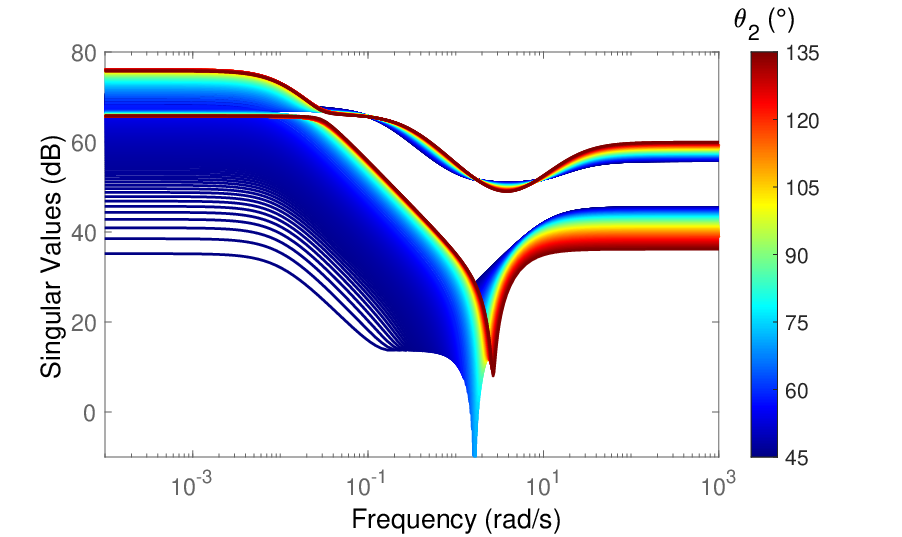
To validate the proposed approach, the model of the same robotic arm is built with Simscape Multibody and linearized around the equilibrium. The proposed LFT model matches Simscape’s model in the nominal configuration of the uncertain parameters and across all angular configurations, as shown in Fig. 5, where the relative error between the two models stays small even in the worst-case configurations around $\bar{\theta}_{1}=\pm$90\text{\,}\mathrm{\SIUnitSymbolDegree}$$. Non nominal configurations were also tested and matched the corresponding Simscape’s model. Moreover, Fig. 6 presents the singular values of the transfer $[\delta T_{1}\,,\,\delta T_{2}]^{T}\rightarrow[\delta\theta_{1}\,,\,\delta\theta_{2}]^{T}$ for both models in one angular configuration. Let us emphasize that the proposed LFT model contains all configurations of the scheduling parameters $t_{1}$ and $t_{2}$ as well as the parametric uncertainties in one single model, while the Simscape model needs to be reevaluated, trimmed and linearized for every geometric or parametric configuration.

To conclude, a robust LPV controller is proposed to illustrate the compatibility of the proposed approach with classical robust control tools and to show the advantages of the LFT model. The angles are limited to the following operating ranges: $\theta_{1}\in\left[$45\text{\,}\mathrm{\SIUnitSymbolDegree}$,$90\text{\,}\mathrm{\SIUnitSymbolDegree}$\right]$ and $\theta_{2}\in\left[$45\text{\,}\mathrm{\SIUnitSymbolDegree}$,$135\text{\,}\mathrm{\SIUnitSymbolDegree}$\right]$, and the set of scheduling parameters is noted $\bm{\tau}=\left\{t_{1},t_{2}\right\}$.

Noting $\delta\bm{\theta}_{\mathrm{ref}}=[\delta\theta_{1}^{\mathrm{ref}}\,,\,\delta\theta_{2}^{\mathrm{ref}}]^{T}$ the vector of reference angles, $\delta\mathbf{e}=\delta\bm{\theta}_{\mathrm{ref}}-[\delta\theta_{1}\,,\,\delta\theta_{2}]^{T}$, and $\delta\mathbf{T}=[\delta T_{1}\,,\,\delta T_{2}]^{T}$, the LPV controller $\mathbf{K}(\mathrm{s},\bm{\tau})$ is such that:

Let the real matrices of appropriate dimensions $\mathbf{A}(\bm{\tau})$, $\mathbf{B}(\bm{\tau})$, $\mathbf{C}(\bm{\tau})$, $\mathbf{D}(\bm{\tau})$ define the state-space representation of $\mathbf{K}(\mathrm{s},\bm{\tau})$. The scheduling surface $\mathbf{S}(\bm{\tau})$ is defined as:

where the matrices $\mathbf{M}_{0}$, $\mathbf{M}_{1}$, $\mathbf{M}_{2}$ are to be tuned, and the LPV controller $\mathbf{K}(\mathrm{s},\bm{\tau})$ reads:

where $\mathcal{F}_{u}$ refers to the upper LFT, $n_{s}$ is the number of states of the controller, and the block $\Delta^{K}_{\bm{\tau}}$ isolates the occurrences of $t_{1}$ and $t_{2}$.

The value $n_{s}=3$ was chosen, and after defining the weighting functions $\mathbf{W}_{T}=1/1500\,\mathbf{I}_{2}$ (to limit the actuator’s efforts) and $\mathbf{W}_{e}(\mathrm{s})=\frac{\mathrm{s}+1}{2\mathrm{s}+0.02}\,\mathbf{I}_{2}$ (to penalize low-frequency tracking error), the robust, structured $\mathcal{H}_{\infty}$ problem:

was solved with Matlab routine systune, based on the algorithm presented in [17]. A performance ($\gamma_{1}=0.97$, $\gamma_{2}=0.69$) was obtained (corresponding to the worst-case $\mathcal{H}_{\infty}$ norms of the transfers), and Fig.7 represents the LPV controller. Since the proposed modeling approach provided all parametric configurations of both the uncertain and scheduling parameters in one single LFT model, the robustness and the LPV controller synthesis were addressed together in one single control design iteration, and the resulting performance is guaranteed across all parametric configurations.

References

- [1] B. Rong, X. Rui, L. Tao, and G. Wang, “Theoretical modeling and numerical solution methods for flexible multibody system dynamics,” Nonlinear Dynamics, vol. 98, no. 2, pp. 1519–1553, 2019.
- [2] K. Zhou, J. C. Doyle, and K. Glover, Robust and Optimal Control. Prentice hall, 1996.
- [3] A. Marcos, D. G. Bates, and I. Postlethwaite, “Exact nonlinear modelling using symbolic linear fractional transformations,” IFAC Proceedings Volumes (IFAC-PapersOnline), vol. 16, pp. 190–195, 2005.
- [4] Z. Szabó, A. Marcos, D. Mostaza Prieto, M. L. Kerr, G. Rödönyi, J. Bokor, and S. Bennani, “Development of an integrated LPV/LFT framework: Modeling and data-based validation tool,” IEEE Transactions on Control Systems Technology, vol. 19, no. 1, pp. 104–117, 2011.
- [5] H. Pfifer and S. Hecker, “Generation of optimal linear parametric models for LFT-based robust stability analysis and control design,” IEEE Transactions on Control Systems Technology, vol. 19, no. 1, 2011.
- [6] C. Roos, G. Hardier, and J. M. Biannic, “Polynomial and rational approximation with the APRICOT Library of the SMAC toolbox,” 2014 IEEE Conference on Control Applications, CCA 2014, 2014.
- [7] D. Alazard, C. Cumer, and K. Tantawi, “Linear dynamic modeling of spacecraft with various flexible appendages and on-board angular momentums,” 7th International ESA Conference on Guidance, Navigation and Control Systems, vol. 41, no. 2, pp. 11 148–11 153, 2008.
- [8] D. Alazard and F. Sanfedino, “Satellite Dynamics Toolbox for Preliminary Design Phase,” 43rd Annual AAS Guidance and Control Conference, vol. 172, pp. 1461–147, 2020.
- [9] D. Alazard, J. A. Perez, T. Loquen, and C. Cumer, “Two-input two-output port model for mechanical systems,” in AIAA Guidance, Navigation, and Control Conference, 2013. Reston, Virginia: American Institute of Aeronautics and Astronautics, jan 2015.
- [10] F. Sanfedino, D. Alazard, V. Pommier-Budinger, A. Falcoz, and F. Boquet, “Finite element based N-Port model for preliminary design of multibody systems,” Journal of Sound and Vibration, vol. 415, 2018.
- [11] F. Sanfedino, V. Preda, V. Pommier-Budinger, D. Alazard, F. Boquet, and S. Bennani, “Robust Active Mirror Control Based on Hybrid Sensing for Spacecraft Line-of-Sight Stabilization,” IEEE Transactions on Control Systems Technology, vol. 29, no. 1, 2021.
- [12] J. A. Perez, C. Pittet, D. Alazard, and T. Loquen, “Integrated Control/Structure Design of a Large Space Structure using Structured Hinfinity Control,” IFAC-PapersOnLine, vol. 49, no. 17, 2016.
- [13] E. Kassarian, F. Sanfedino, D. Alazard, H. Evain, and J. Montel, “Modeling and stability of balloon-borne gondolas with coupled pendulum-torsion dynamics,” Aerospace Science and Technology, vol. 112, 2021.
- [14] P. Zipfel, Modeling and Simulation of Aerospace Vehicle Dynamics. American Institute of Aeronautics and Astronautics, 2014.
- [15] V. Dubanchet, “Modeling and Control of a Flexible Space Robot to Capture a Tumbling Debris,” Ph.D. dissertation, Ecole Polytechnique de Montréal, 2016.
- [16] A. Varga and G. Looye, “Symbolic and numerical software tools for LFT-based low order uncertainty modeling,” Proceedings of the IEEE International Symposium on Computer-Aided Control System Design, no. 1, pp. 1–6, 1999.
- [17] P. Apkarian and D. Noll, “Nonsmooth H infinity synthesis,” IEEE Transactions on Automatic Control, vol. 51, no. 1, pp. 71–86, 2006.