No umbrella needed: Confronting the hypothesis of iron rain on WASP-76b with post-processed general circulation modelsJournal: The Astrophysical Journalastropy (Price-Whelan et al. 2018), batman (Kreidberg 2015), Corner (Foreman-Mackey 2016), emcee (Foreman-Mackey et al. 2013), exoplanet (Foreman-Mackey et al. 2021), FastChem (Stock et al. 2018), IPython (Pérez & Granger 2007), Matplotlib (Hunter 2007), NumPy (Harris et al. 2020), Numba (Lam et al. 2015), pandas (McKinney 2010), SciPy (Virtanen et al. 2020), tqdm (da Costa-Luis 2019)
Abstract
High-resolution spectra are unique indicators of three-dimensional processes in exoplanetary atmospheres. For instance, in 2020, Ehrenreich et al. reported transmission spectra from the ESPRESSO spectrograph yielding an anomalously large Doppler blueshift from the ultra-hot Jupiter WASP-76b. Interpretations of these observations invoke toy model depictions of gas-phase iron condensation in lower-temperature regions of the planet’s atmosphere. In this work, we forward model the atmosphere of WASP-76b with double-gray general circulation models (GCMs) and ray-striking radiative transfer to diagnose the planet’s high-resolution transmission spectrum. We confirm that a physical mechanism driving strong east-west asymmetries across the terminator must exist to reproduce large Doppler blueshifts in WASP-76b’s transmission spectrum. We identify low atmospheric drag and a deep radiative-convective boundary as necessary components of our GCM to produce this asymmetry (the latter is consistent with existing Spitzer phase curves). However, we cannot reproduce either the magnitude or the time-dependence of the WASP-76b Doppler signature with gas-phase iron condensation alone. Instead, we find that high-altitude, optically thick clouds composed of , Fe, or provide reasonable fits to the Ehrenreich et al. observations — with marginal contributions from condensation. This fit is further improved by allowing a small orbital eccentricity (), consistent with prior WASP-76b orbital constraints. We additionally validate our forward-modeled spectra by reproducing lines of nearly all species detected in WASP-76b by Tabernero et al. 2021. Our procedure’s success in diagnosing phase-resolved Doppler shifts demonstrates the benefits of physical, self-consistent, three-dimensional simulations in modeling high-resolution spectra of exoplanet atmospheres.
Keywords:
Exoplanet atmospheric composition (2021) — Radiative transfer simulations (1967) — High resolution spectroscopy (2096) — Hot Jupiters (753)I Introduction
Decades after the discovery of the first exoplanet (Mayor & Queloz 1995), a harbinger of the population of “hot Jupiters,” observational, theoretical, and laboratory efforts have elucidated some of the key processes and features relevant to these planets (Showman & Guillot 2002; Cooper & Showman 2006; Knutson et al. 2007; Fortney et al. 2008; Crossfield et al. 2010; Rauscher & Menou 2012; Dobbs-Dixon & Agol 2013; Demory et al. 2013; Kataria et al. 2015; Mendonça et al. 2016; Fleury et al. 2019; Winter et al. 2020, e.g.,). In the past five years, however, an even more extreme class of planet — the “ultra-hot Jupiter” (Bell & Cowan 2018; Arcangeli et al. 2018; Parmentier et al. 2018) — has emerged, once again requiring the construction of new theoretical frameworks. Featuring persistent dayside temperatures in excess of 2200 K, ultra-hot Jupiter atmospheres are thought to include thermal dissociation of molecules and thermal ionization of metals. The presence of gas-phase metals at low pressures within these atmospheres also renders ultra-hot Jupiters notably susceptible to temperature inversions by virtue of strong optical absorption of host star light (Lothringer & Barman 2019, e.g.,). In short, observations of ultra-hot Jupiters have revealed them to be sites for extreme physics, consequently requiring significant model updates to understand them in detail.

One particularly intriguing aspect of ultra-hot Jupiter atmospheres is their three-dimensional (3-D) structure. Such highly irradiated objects are predicted to have very strong day-night temperature gradients, and perhaps chemical gradients, too (Showman et al. 2009; Rauscher & Menou 2012; Kataria et al. 2016, e.g.,); these atmospheres’ short chemical timescales relative to dynamical timescales should drive them to chemical equilibrium (Baeyens et al. 2021). These features make it challenging to justify treating such planets as 1-D objects, and the departures from 1-D behavior are especially apparent in certain current and future (Feng et al. 2020; Taylor et al. 2020; Pluriel et al. 2020; MacDonald et al. 2020) observations, including those at high spectral resolution, which are the subject of this paper.
To account for the unique 3-D properties of ultra-hot Jupiters, various updates to “traditional” hot Jupiter general circulation models (GCMs) have been required. For instance, recent models have incorporated the cooling and heating effects of hydrogen dissociation and recombination (Tan & Komacek 2019; Mansfield et al. 2020). Moreover, the Lorentz forces and Ohmic dissipation related to free electrons in weakly ionized atmospheres have been captured to varying degrees of sophistication in GCM frameworks, often as a Rayleigh drag force (Perna et al. 2010; Rauscher & Menou 2013; Komacek & Showman 2016, e.g.,) or by coupling to the magnetic induction equation (Batygin et al. 2013; Rogers & Showman 2014; Hindle et al. 2019; Hindle et al. 2021). Finally, the net thermal flux at the lower boundary can substantially impact the GCM-predicted thermal structure and circulation higher in the atmosphere (Rauscher & Menou 2012; Showman et al. 2015, e.g.,), making this parameter a useful tuning knob to explore the effect of differing interior entropies on global dynamics.
In terms of observing the unique characteristics of ultra-hot Jupiters, ground-based high-resolution spectroscopy offers a wealth of information related to their thermal, chemical, aerosol, and dynamical (i.e., wind) structures and properties (Snellen et al. 2013; Kempton et al. 2014; Brogi et al. 2016; Hood et al. 2020, e.g.,). Like traditional transmission spectroscopy, observations at high spectral resolution make use of the fact that host star light filtered through an exoplanet’s atmosphere will be preferentially absorbed by certain chemical species at certain wavelengths. Instead of necessarily dividing in-transit by out-of-transit spectra, high-resolution spectra can be extracted by noting that the stellar lines (and telluric lines from the Earth’s atmosphere) will be essentially stationary during the planet’s transit, modulo the host star’s planet-induced acceleration relative to the Earth. In contrast, lines associated with the planet can be individually resolved and will Doppler shift over the course of the planet’s transit because of the planet’s orbital motion, winds, and rotation (Snellen et al. 2010). Ultra-hot Jupiters are therefore favorable targets for high-resolution spectroscopy; in addition to being likely to transit (Seagroves et al. 2003, e.g.,), their short orbital periods ensure that their lines undergo appreciable Doppler shifts over the course of their transit, making the planetary spectrum easier to disentangle. Moreover, ultra-hot Jupiters have large atmospheric scale heights due to their low mean molecular weight and high temperatures, which increase their signal strengths in transmission.
Although hot Jupiter spectra derived from 1-D and 3-D modeling tend to generally agree in their interpretation of current low-resolution data (Fortney et al. 2010), significant departures — containing information about wind fields, thermal profiles, and planetary rotation — begin to crop up at higher resolution (Kempton & Rauscher 2012; Showman et al. 2013; Kempton et al. 2014; Flowers et al. 2019; Beltz et al. 2020). Together, then, GCMs and high-resolution radiative transfer modeling can work synergistically to generate spectra that consider the full 3-D nature of the underlying atmosphere.
A prime example of the unique benefits of the intersection of the 3-D nature of (ultra-)hot exoplanet atmospheres and high-resolution spectroscopy lies in the ultra-hot Jupiter WASP-76b, a gas giant orbiting an F7 star (West et al. 2016) that is well-studied at lower resolution (Fu et al. 2017; Tsiaras et al. 2018; Fisher & Heng 2018; Edwards et al. 2020; von Essen et al. 2020; Fu et al. 2021). Using the high-resolution (R 138,000) ESPRESSO spectrograph on the VLT (Pepe et al. 2010; Pepe et al. 2013), the Ehrenreich et al. 2020 team was able to produce novel, high-SNR, phase-resolved transmission spectra of this target across two separate transits. Curiously, an anomalous Doppler signature in the planet’s transmission spectrum was detected: between 0 and km s-1 at ingress, but roughly km s-1 by egress. These speeds far exceed the few km s-1 planet-frame velocities detected on other planets (Snellen et al. 2010; Brogi et al. 2016). The detection team attributes this variable and strong blueshift to an asymmetric distribution of atomic iron in the planet’s atmosphere, with a considerable amount of iron existing in the gas phase east of the substellar point but cooling and condensing out as it makes its way to the much colder nightside. This asymmetry would cause a progressively blueshifted signal as the gas-phase iron region rotates into view over the course of the planet’s transit. Ehrenreich et al. 2020 posit that their signal is composed of two independent Doppler components: solid-body rotation of 5.3 km s-1, the tidally locked equatorial velocity of the planet, and a uniform day-night wind contributing an additional km s-1 across both limbs, with gas phase iron only present on the evening limb of the planet (Figure 1). Hence, the approaching limb would exhibit a blueshift from both rotation and winds totaling –10.6 km s-1, and the receding limb would produce no Doppler signal, as it would contain no gas-phase iron to absorb starlight.
The Ehrenreich et al. 2020 “toy model,” as they put it, is supported by a separate, archival analysis of HARPS data (Kesseli & Snellen 2021), which similarly finds increasing blueshift over the course of WASP-76b’s transit. Additionally, the magnitude of the blueshift and speed of the day-night flow are confirmed by Tabernero et al. 2021 and Seidel et al. 2021, who perform in-depth secondary analyses of the Ehrenreich et al. 2020 dataset. These works also produce rich datasets in their own right, with the Tabernero et al. 2021 study reporting the detection of multiple chemical species (Li I, Na I, Mg I, Ca II, Mn I, K I), their atmospheric heights, and their corresponding blueshifts.
The aforementioned iron chemistry gradient interpretation would be the first of its kind among exoplanet atmospheres. However, the necessity of a chemical gradient to explain the extant observations has been questioned by the forward models of Wardenier et al. 2021, who self-consistently calculate transmission spectra from a 3-D model of this planet and find that either iron condensation or a significant temperature asymmetry could match the Ehrenreich et al. 2020 data. Furthermore, Fe clouds are not necessarily favored in hot Jupiter atmospheres; microphysics models indicate that the nucleation rate of Fe is low, causing Fe clouds to be sequestered deep in the atmosphere (Gao et al. 2020; Gao & Powell 2021).
In this paper, in addition to seeking to examine the iron rain hypothesis, we also aim to understand the physical, chemical, and dynamic processes at play in the atmosphere of WASP-76b. We do so with a suite of GCM simulations, applying a spectroscopic post-processing scheme to evaluate the likelihood of several plausible physical scenarios in the face of the constraints provided by the Ehrenreich et al. 2020, Tabernero et al. 2021, and Kesseli & Snellen 2021 data. Our companion paper, \hyper@natlinkstartmaykomacek2021spitzerMay & Komacek et al.\hyper@natlinkend (May et al. 2021), examines the dynamics of this planet with the aid of Spitzer phase curves; this paper focuses on the detected blueshift signature and chemical species by post-processing GCM simulations to produce high-resolution transmission spectra. Together, these works aim to compare the results of photometric phase curves and high-resolution transmission spectroscopy to paint a coherent picture of WASP-76b’s 3-D atmosphere.


This paper is organized as follows. Section II describes the setup of our GCM and radiative transfer models, as well as the various physical scenarios we explore. Section III then lays out the analysis that we perform on the resultant spectra, which allows us to make direct comparisons to the Ehrenreich et al. 2020 and Tabernero et al. 2021 observational work. We present these comparisons in Section IV, along with physical motivation for the individual effects included in our modeling results. Next, Section V briefly explores further alternative explanations for the anomalous blueshift and places our results in the context of other work. Finally, we summarize our conclusions in Section VI.
| Parameter | Value(s) | Unit |
| 1.30 | m | |
| 6.4 | ||
| 1.22 | m | |
| 1.81 | days | |
| , 33 3 Limb-darkening coefficients assume a quadratic law. | 0.393, 0.219 | N/A |
| 6329 | K | |
| 3, 4, 5, 6, 7 | s | |
| RCB | Shallow, deep | N/A |
| Cloud composition44 4 All clouds are modeled as fully optically thick. | Fe, , | N/A |
| Max. cloud extent | 1, 5, 10 | scale heights |
| Condensation55 5 Gas-phase iron condensation is treated independently from cloud formation. | on, off | N/A |
| Orbital phase, | (, 15.4) | degrees |
| Orbital eccentricity, | (0.0, 0.05) | N/A |
| Lon. of periastron, | (0, 360) | degrees |
II Model description
II.1 GCM
As described above, we aim to produce physically motivated, self-consistent comparisons to the Ehrenreich et al. 2020 data by spectrally post-processing the outputs of a GCM. We use the same GCM model introduced and described in detail in our companion paper, which also includes the full GCM parameter assumptions and values (\hyper@natlinkstartmaykomacek2021spitzerMay & Komacek et al.\hyper@natlinkend May et al. 2021, Table 3). Broadly, we use the MITgcm (Adcroft et al. 2004) to solve the primitive equations of meteorology on a cubed-sphere grid with a horizontal resolution of C48 and 70 vertical layers, extending evenly in log-pressure from 100 bars to 10 microbars. To connect the modeled atmospheric circulation to heating and cooling within the atmosphere, the GCM is coupled with a two-stream, double-gray radiative transfer scheme with the TWOSTR (Kylling et al. 1995) package of DISORT (Stamnes et al. 1988). A crucial update warranted for this project is the inclusion of local cooling where hydrogen dissociates, relevant to the intense dayside stellar irradiation of ultra-hot Jupiters, and local heating at locations where atomic hydrogen recombines, relevant to the much cooler limbs and nightsides of ultra-hot Jupiters (Tan & Komacek 2019; Mansfield et al. 2020).
As described in our companion paper (\hyper@natlinkstartmaykomacek2021spitzerMay & Komacek et al.\hyper@natlinkend May et al. 2021), our GCMs (Figure 2) incorporate a spatially constant Rayleigh drag force proportional to , for horizontal wind velocity and drag timescale . Our grid of GCMs encompasses a parameter sweep of drag timescales and two endmembers of radiative-convective boundary (RCB) depth, with the aim of exploring a wide range of possible dynamical states and interior states of WASP-76b. Our models are computed over a parameter sweep of drag timescales ( [s, s], with five values sampled evenly in log space), motivated by the unknown strength of turbulence and magnetic forces associated with the ionized dayside. The longest drag timescales correspond to atmospheres that have similar temperature structures and wind speeds to those with no applied frictional drag. We model upward heat fluxes from the deep planetary interior by including a “surface” beneath our model domain that does not interact with the atmospheric flow aside from heating it. The upward fluxes for our limiting cases of RCB depth are (= 500 K) and (= 5300 K) for the deep and shallow RCB cases, respectively.
II.2 Radiative transfer model
II.2.1 Overview
For our study, we make use of a line-of-sight ray-striking radiative transfer model that includes Doppler effects, inherited from Kempton & Rauscher 2012, Kempton et al. 2014, Rauscher & Kempton 2014, and Flowers et al. 2019. We begin with the GCM output, which we interpolate from a grid evenly spaced in pressure onto a grid evenly spaced in altitude — thus ensuring that our simulated rays propagate in straight lines. We further only consider the GCM output at pressures generally greater than 1 bar (the cut is made in altitude, not pressure, so the bottom-most pressure value is weakly latitude/longitude dependent), as the atmosphere is fully optically thick in transmission geometry at pressures greater than this value (Figure 3). We convert between pressure and altitude assuming hydrostatic equilibrium, accounting for the non-uniform mean molecular weight between GCM grid cells due to the thermal dissociation of H2 in hotter regions of the atmosphere. Our calculation assumes a nominal atmosphere in cooler regions that is 83.6% H2, 16% He, and 0.4% metal-bearing molecules (the latter having an average mean molecular weight ) by number.
Accounting for the 3-D geometry of our GCM structures, we calculate the slant optical depth,
| (1) |
along a given trajectory after determining the opacity in each grid cell as a local function of temperature and pressure (see Section II.2.2 for a discussion of our opacity sources), where is the line-of-sight path length through an individual grid cell. The wavelength at which is evaluated is adjusted depending on the line-of-sight velocity of the grid cell , as per
| (2) |
for rest wavelength , east-west velocity , north-south velocity , latitude , longitude , altitude , speed of light , and planetary angular rotation speed . These Doppler shifts assume that the orbital velocity of the planet has already been entirely accounted for; we address potential consequences of this assumption with respect to WASP-76b in Section V.2.1. As described in Kempton & Rauscher 2012, higher-order line-shifting effects such as gravitational redshifting and microturbulent broadening are expected to be negligible.

After calculating the above , we can calculate the intensity along each line of sight, assuming absorption-only radiative transfer:
| (3) |
for stellar intensity incident upon a grid cell, . We assume that the stellar spectrum follows a blackbody distribution for K, the effective temperature of WASP-76 (Ehrenreich et al. 2020). The total flux transmitted through the atmosphere is arrived at by integrating over the sky-projected solid angle of each respective grid cell through which a beam emerges. The wavelength-dependent transit depth is then given by
| (4) |
where is the out-of transit flux (i.e. the stellar flux) and is the in-transit flux, accounting for both the blockage of stellar light by the optically thick core of the planet and the transmitted flux through the atmosphere.
Our spectral simulations are computed over the 379 – 789 nm range to coincide with the ESPRESSO data from Ehrenreich et al. 2020, with a total of 298,766 individual wavelength points corresponding to a resolution of . After computation, our spectra are convolved to the native ESPRESSO resolution in the singleHR mode (Pepe et al. 2013, ;). Because of very large file sizes and RAM requirements associated with the substantial number of wavelength points, we generate the spectra in discrete wavelength “chunks” on a high-performance computing cluster and then stitch the entire spectrum together once the full calculation is complete.
II.2.2 Opacity sources
Because WASP-76b is an ultra-hot Jupiter observed at optical wavelengths, we compile a set of opacities that is appropriate for these conditions. The atomic species that we utilize are Fe I, Fe II, Mg I, Mn I, Na I, Ca II, Ti, Li I, and K I; and our molecular species are TiO, VO, OH, and . Rayleigh scattering from H2, H, and He, as well as bound-free and free-free absorption are included as continuum opacity sources. Finally, collision-induced opacity from collisional pairs of -, -H, -He, and H-He is considered. This list of opacity sources includes all of the species with reported detections in WASP-76b optical spectra from Ehrenreich et al. 2020, Tabernero et al. 2021, and Fu et al. 2021. We do not include ZrO, which was searched for in WASP-76b by Tabernero et al. 2021 but resulted in a non-detection. In modeling WASP-76b, we generate two sets of transmission spectra, one with Fe (I and II) and continuum opacity sources only, and another with the full set of molecular, atomic, and continuum absorbers (see Figure 4 and Section IV.1.1).
All opacities are generated on a temperature-pressure grid spanning from 500 – 5000 K and 1 – 1 bar, covering the range of the WASP-76b GCM output. We initially calculate opacities on an evenly spaced wavenumber grid, from a wavenumber of 0 to 30,000 with a spacing of 0.01 . These results are then downsampled with the k-table feature of HELIOS (Malik et al. 2017).
We use the newest available open-source line lists in constructing our molecular opacities: VO (McKemmish et al. 2016, VOMYT;), TiO (McKemmish et al. 2019, TOTO;), OH (Tennyson et al. 2016, MoLLIST;), (Polyansky et al. 2018, POKAZATEL;). Atomic opacities are drawn from the Kurucz database (Kurucz 1995). In selecting our opacities, we make use of the most abundant isotopologue for each species. Our atomic sources do not include pressure broadening --- only Doppler (thermal) and natural broadening.66 6 The Doppler effects from planetary rotation and winds dominate over the broadening introduced by pressure, thermal, and quantum effects here, because the signal for high-resolution spectra originates from high-altitude, low-pressure regions of planetary atmospheres. Furthermore, our science case is primarily concerned with the location of line centers, not the exact nature of line wings. Therefore, we anticipate that the exclusion of pressure broadening here does not significantly impact our final spectra. From these line lists, we calculate the relevant opacities with the GPU-enabled HELIOS-K code (Grimm & Heng 2015).
Opacities from individual species are combined by a weighting of their respective mixing ratios, under the assumption that the atmosphere of WASP-76b resides in a state of chemical equilibrium. To determine the chemical equilibrium mixing ratios, we employ the FastChem model (Stock et al. 2018), which accounts for gas-phase chemistry only. In Section II.2.4, we describe how we treat condensation for the purposes of our modeling.
II.2.3 Phase-dependent transmission spectra
As in Flowers et al. 2019, to compare our model transmission spectra directly against the Ehrenreich et al. 2020 results, we must calculate transmission spectra as a function of orbital phase throughout the duration of transit. To account for orbital phase dependencies, we apply the following procedure:
- 1.
Account for phase-dependent back-lighting of the planet (i.e. stellar limb-darkening effects). At different points of its transit, the planet will occult regions of its host star of varying brightness. Furthermore, at a fixed orbital phase, different regions of the planet’s limb will be back-lit by varying intensities of stellar light. Similarly to Flowers et al. 2019, we calculate the normalized stellar intensity at the center of each cell of the 2-D projected planetary grid produced by our GCM at each modeled orbital phase of the planet. We use the quadratic limb-darkening coefficients reported by Ehrenreich et al. 2020 to establish the stellar center-to-limb intensity profile, and we take into account the 89.623∘ orbital inclination of WASP-76b (Ehrenreich et al. 2020) to determine where the planet resides on the stellar disk as a function of its orbital phase. We make the assumption of constant impact parameter over the course of transit.77 7 In reality, a planet on an inclined orbit will not have a constant over the entire duration of transit; rather, the planet’s distance from the stellar equator will be decreased at ingress and egress, reaching its maximum at center of transit. Our tests reveal that the relative error induced by the constant assumption is on the order of 4% in distance, which results in a change on the order of 1 m/s at the blueshift level (see Section III.1). Hence, our treatment is justified. This procedure allows us to calculate a back-lighting factor , which ranges from 0 to 1, effectively replacing the constant from Equation 3 with a variable , for a given orbital phase and 2-D projected polar angle .
- 2.
Account for the decreasing of the continuum by interpolating a light curve produced by the batman code (Kreidberg 2015). Step 1 ensures that less light is transmitted through the planet’s atmosphere than a uniform stellar disk would emit. Step 2 further enforces that the inner, optically thick core of the planet is simulated crossing a limb-darkened star, as opposed to a star of uniform brightness.
- 3.
Account for the planet’s rotation over the course of transit. Because the planet is continually rotating as it travels across the face of its host star, we must transform the GCM coordinate system so that the correct observer-facing hemisphere is modeled at each instance during transit. For simplicity, we assume zero obliquity, which allows us to calculate the coordinate transform simply by assigning a linear offset to each planetary longitude; i.e., .
In choosing phases at which to evaluate our models, we more densely sample ingress and egress because the transmission signal quickly varies in strength and velocity during these times. The sampling that we employ is:
| (5) |
where represents the phase at which the planet’s trailing limb no longer occults the stellar disk. This procedure results in 50 total orbital phases being explicitly modeled with our radiative transfer post-processing code.
II.2.4 Condensation and clouds
The large blueshifts observed by Ehrenreich et al. 2020 have been attributed to iron condensation on the nightside and cooler “morning” limb of WASP-76b. To confront this hypothesis within the framework of our transmission spectrum modeling, we account for clouds and condensation in the following ways.
To incorporate the effects of condensation out of the gas phase, we utilize the iron condensation curve for a solar composition mixture computed in Mbarek & Kempton 2016. At each cell in our GCM-produced atmosphere, we interpolate the condensation curve at the cell’s pressure; if the temperature in the cell is lower than the interpolated condensation temperature, then we remove iron from the total opacity calculation at that location by setting its opacity contribution to zero. This approach maximizes the effect of Fe condensation, as in reality homogeneous nucleation of Fe is inefficient (Gao & Powell 2021). This step effectively treats the physics considered in the Ehrenreich et al. 2020 toy model, which only accounted for gas phase removal as the process responsible for the large net blueshifts in WASP-76b’s transmission spectrum.
In our full-species modeling of WASP-76b’s transmission spectrum, we allow other species to condense out of the atmosphere following a similar procedure. We condense Ca (I and II) following the condensation curve, Ti and TiO following , K following , Na following , Mn following MnS, and Cr following . Our prescription of complete removal implies full rainout from the gas phase once the species-limiting condensate forms.
Condensation not only causes gas-phase depletion but can also result in the formation of an optically thick cloud made up of liquid droplets or solid particles. Such a cloud layer would block transmission of stellar light through the atmosphere in the location where the cloud forms and could therefore also be the main driver of the “missing” iron absorption in the receding limb of WASP-76b’s atmosphere — a scenario that has not yet been explored in the literature for this planet. To account for such cloud layers, our models further contain a post-processing implementation of gray, optically thick clouds. These clouds, which are self-consistent with our radiative transfer (but not with our GCMs), are placed such that they span up to several () scale heights above the condensation curve of iron, forsterite (), or aluminum oxide ().
Fe is selected because it is the species that is putatively condensing in WASP-76b’s atmosphere; is modeled because per the microphysics model of Gao et al. 2020, silicate clouds are chemically favored over iron ones and appear to be a defining feature in the transmission spectra of giant planets with comparable irradiation to WASP-76b; and is considered because it is the highest-temperature condensate predicted in hot Jupiter atmospheres (Mbarek & Kempton 2016).
Notably, our implemented clouds never fully reach the limiting-case thickness of 10 scale heights. Because our temperature-pressure profiles tend to cross condensation curves twice (Figure 2), clouds cannot exist in the uppermost regions of the atmosphere — the upper boundary of the cloud is (indirectly) set by the pressure at which the atmospheric inversion or isothermal region occurs. This effect can be seen in the bottom row of Figure 5, in which the “10 scale height” clouds do not extend much past the “1 scale height” clouds. Hence, while our clouds can exist up to 10 scale heights in thickness (provided they fulfill their criterion with respect to a given condensation curve), in practice they are limited by the temperature/pressure structure of the atmosphere.

Similarly to our condensation treatment, our cloud effect is modeled post-hoc, in that the radiative effects of cloud formation and the resultant changes to opacities are not accounted for natively in the GCM (see Section V.3 for a discussion of this limitation). Furthermore, our simple cloud model does not account for the wavelength-dependent scattering and/or absorption from cloud particles — a simplification that is justified because cloud opacities are typically smoothly varying with wavelength, in contrast with the sharply wavelength-dependent atomic and molecular features that are primarily responsible for the high-resolution transmission spectrum signal in cross-correlation. Additionally, cloud particle sizes are represented by broad distributions, and no clouds in a planetary atmosphere are characterized by a single particle size (Pont et al. 2013, e.g.,).
II.3 Suite of models
The suite of post-processed spectral models explored in this work is laid out in Table 2. We use the following terminology to refer to our various model implementations. By “condensation on,” we mean that we are applying the rainout prescription described in Section II.2.4. “Fe-only” models refer to those in which the only non-continuum opacity source is gas-phase iron. Our “full-species” models include the full set of opacities listed in Section II.2.2.
Furthermore, when referring to cloud inclusion, “Fe clouds on” implies the placement of an optically thick cloud above the Fe condensation curve with a thickness equivalent to a specified number of scale heights. Similarly, “” or “ clouds on” refer to the same, albeit above the or condensation curves, respectively. The inclusion of clouds in our models is decoupled from our condensation procedure, allowing us to model these effects together or separately.
The majority of our work holds WASP-76b on a circular orbit (i.e., = 0). We investigate the effect of eccentric orbits in Section V.2.1.
III Analysis
III.1 Cross-correlation
With our model spectra in hand, our next step is to determine the information that can be recovered from these spectra. For high spectral resolution observations of exoplanet atmospheres, signal recovery has typically been accomplished via a cross-correlation analysis (Snellen et al. 2010; Birkby et al. 2013; Brogi et al. 2016, e.g.,). This procedure has an advantage over the fitting of individual spectral lines (Section III.2) in that it leverages a key aspect of high-resolution data — a forest of weak lines that together can produce a high-SNR detection of a chemical species. To mimic the data analysis process undertaken by Ehrenreich et al. 2020, thereby allowing us to compare our models directly to their results, we implement a cross-correlation procedure into our modeling routine.
Our cross-correlation function (CCF) is computed by combining our data, , with a mask or template, , at a given velocity, , as follows (Baranne et al. 1996; Pepe et al. 2002; Allart et al. 2017; Hoeijmakers et al. 2019, e.g.,):
| (6) |
where the mask or template is Doppler-shifted by velocity and interpolated onto the wavelength grid of for summing. This calculation produces a map of cross-correlation against velocity (Figure 6); the location of the peak of this distribution is reported as the net Doppler shift of . We Doppler-shift between km s-1 and 250 km s-1 in steps of 1 km s-1.
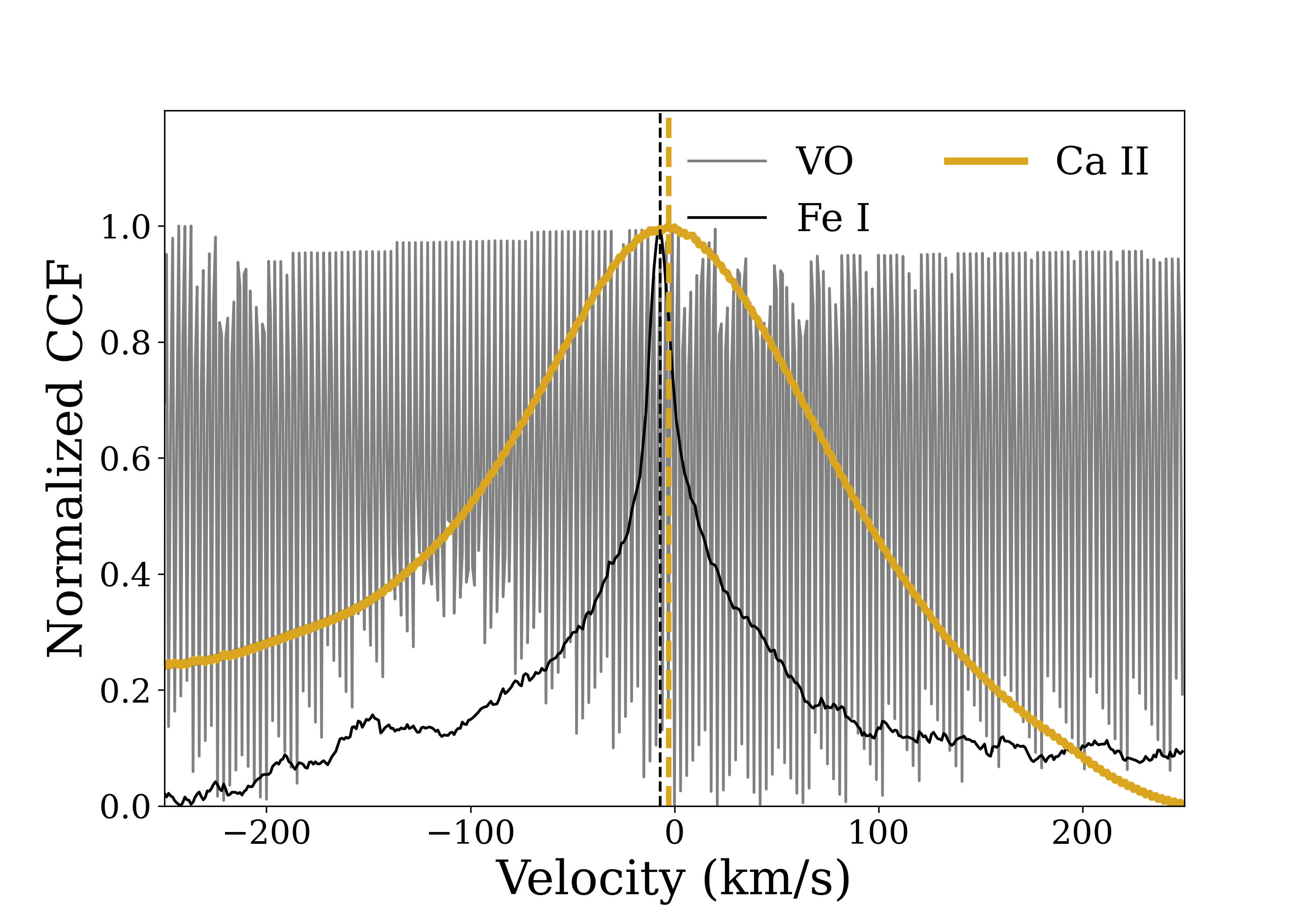
We first employ a model-on-model cross-correlation. To do so, we construct as our template a simplified, “Doppler-off” spectrum, which is a model otherwise equivalent to the simulated data but with no Doppler shifts applied in the radiative transfer calculation. This template is then convolved down to the resolution of ESPRESSO using a Gaussian kernel of appropriate width. We then perform the previously described cross-correlation procedure.
Once we perform our cross-correlation, we fit a Gaussian to our CCF with the SciPy curve_fit routine. The peak value of the fitted Gaussian is then reported as the velocity shift of a given spectrum.
For CCFs with well-characterized peaks, we perform a second, narrower Gaussian fit in a window 6 km s-1 wide centered on the peak identified by the previous step. Doing so ensures that asymmetries in the CCF far from the peak do not influence the final determination of the peak value. Our fitting process allows us to report CCF peak values to precision higher than the 1 km s-1 sampling of our CCFs; limited testing of sampling CCFs at higher velocity resolution yielded results consistent with our chosen sampling. CCFs that are not well-characterized (e.g., VO; Figure 6) are not considered in further analysis.
III.2 Individual line-fitting
For certain strong lines, we perform individual fitting to determine Doppler shifts of those lines. This process is an important complement to the cross-correlation procedure described above, and it allows us to compare our forward models directly to the observational results of Tabernero et al. 2021, who focused on specific strong lines of a range of chemical species. Individual-line Doppler shifts are also scientifically interesting because lines of different strengths probe different altitudes of the planet’s atmosphere, and hence different portions of the planet’s wind field and temperature structure (Kempton & Rauscher 2012, e.g.,).
To fit individual lines, we fit a Gaussian profile to a narrow spectral window centered on the line in our center-of-transit spectrum. The corresponding Doppler shift () is calculated by comparing the wavelength at the maximum of the fit Gaussian () to the rest wavelength ():
| (7) |
For ease of comparison to the Tabernero et al. 2021 data, we fit the same lines examined by that study. Furthermore, we adopt their method for fitting weak lines: As an intermediate approach between cross-correlation of many lines and fitting a single line, Tabernero et al. 2021 combine multiple (maximum 5) weak lines in velocity space and fit them jointly to produce a stronger signal. As with that work, we apply this approach for Fe, Mn, and a subset of Mg lines.
This line-fitting method allows us to probe both the Doppler shifts of individual lines and their depths — which in turn establish the altitude at which these lines become optically thick.
IV Results
IV.1 Cross-correlation
IV.1.1 Fe-only
For our first set of results, we perform our analysis on our iron-only transmission spectra.


We find that controlling the drag timescale over our explored parameter range has the strongest first-order effect on Doppler shift over all phases (Figure 7), with the weak drag models providing a much better match to the Ehrenreich et al. 2020 data than the strong drag models. Decreasing the drag timescale in an atmosphere is equivalent to making drag processes more efficient. In the Helmholtz decomposition framework of Hammond & Lewis 2021, about half the day-night heat redistribution in a fiducial hot Jupiter atmosphere is driven by substellar-antistellar flow; shorter drag timescales would serve to slow the speed of this flow, reducing heat transport. The remainder of the day-night heat redistribution, per Hammond & Lewis 2021, is due to rotational flow — e.g., the superrotating equatorial jet. The speed of this jet would similarly suffer directly from a shorter drag timescale. Additionally, per Showman et al. 2013, stronger drag also reduces the pumping of eddy angular momentum onto the dayside equator because drag damps the propagation of planet-scale wave patterns, further decreasing the jet strength. In sum, increased drag reduces longitudinal asymmetries and slows wind speeds, both of which reduce net Doppler shifts in transmission spectra.
As a result of the aforementioned effects, our high-drag models have more homogenized limbs, whereas low-drag models have limbs that are more heterogeneous, with a visible equatorial jet structure (Figures 3, 5, & 8). These features can be seen in our simulated Doppler shifts (Figure 7). The strong drag case has Doppler shifts that are roughly symmetric about the center of transit, with only a slight ( km s-1) blueshift at mid-transit. Moreover, the maximum and minimum of the Doppler shift are both near 4–5 km s-1, which is close to the equatorial rotational velocity of WASP-76b ( 5.3 km s-1). These features are expected for a solely rotationally broadened profile — which would be predicted for the high-drag models, which have weaker winds. Additionally, a clear prediction from Figure 8 is that the strong drag case is redshifted at ingress and blueshifted at egress — as seen in Figure 7.
Similarly, the Fe abundance map (Figure 5) combined with the wind map (Figure 8) explains the behavior of the weak drag case in Figure 7. Namely, the Fe abundance is asymmetrically distributed, preferentially on the eastern limb, where the strongest blueshifts for this model are. Therefore, the model produces Doppler shifts that are not evenly distributed around 0 km s-1 across phase and are more strongly blueshifted, which is more consistent with the Ehrenreich et al. 2020 observations.
Including iron condensation removes the gas-phase iron in the cooler regions of the atmosphere (Figure 5). As can be inferred from our temperature-pressure structure (Figure 2), condensation is primarily confined to the nightside in all our GCMs. Especially in our weak drag models, condensation is less prominent at the equator, whereas it is more prominent at the mid-latitudes and poles. The effect of condensation tends to be marginal, dependent on cloud placement, and not necessarily linear, reflective of the complexities in the 3-D thermal structure of the atmosphere.
We further find that our deep RCB models are a better fit to the data, generating stronger net blueshifts. A shallow RCB is expected to create a more homogeneous atmosphere, because convective motions quickly mix entropy across large spatial scales, reducing day-night temperature contrasts on deep isobars relative to the deep RCB case. Atmospheric circulation in (ultra-)hot Jupiters is driven and supported by day-night pressure gradients (Showman & Guillot 2002, e.g.,), so the smaller day-night contrasts in the shallow RCB case cause winds to be slower. These slower winds in turn decrease east-west limb asymmetries as well as the strength of the blueshift signal (as shown in Figures 7 & 9).
We find that the presence of optically thick clouds, as opposed to gas-phase iron condensation, also strongly and consistently increases the measured blueshift (Figure 7). This is because clouds will preferentially form on the cooler, receding (eastern) limb, hence blocking its contribution to the transmission spectrum; these clouds would lessen the redshift contribution of the receding limb, thereby boosting the measured blueshift.

As seen in Figure 2, condenses out at hotter temperatures than Fe. Hence, placement of clouds above the condensation curve as opposed to the Fe condensation curve results in a cloud deck situated in warmer regions of the atmosphere. The effect of this change at the blueshift level is highly nonlinear, as it depends somewhat strongly on the exact placement (and thickness) of the cloud. Notably, though, the optically thick clouds produce a “jump” in blueshift near a phase of ° that the other models cannot (Figure 7) — a distinct feature of the Ehrenreich et al. 2020 data. While this jump does not extend to the exact observed magnitude, it appears that an cloud deck (or a similarly positioned cloud of arbitrary composition) provides the type of spatial inhomogeneity required to reproduce the Ehrenreich et al. 2020 data in broad strokes.
Interestingly, although the deep RCB / strong drag GCM would have much more condensation in its atmosphere (Figure 2), the deep RCB / weak drag GCM has much stronger blueshifts (Figure 9). It thus appears that the importance of the drag timescale and faster winds leading to more east-west asymmetry “wins out” over the existence of condensation alone.
Our net center-of-transit Doppler shifts are summarized in Figure 9 for all of the model permutations explored. In total, we find that the following effects produce increased blueshifts in WASP-76b’s atmosphere when iron is considered alone: weak drag, deep RCBs, and optically thick clouds composed of Al2O3, Mg2SiO4, or Fe. Gas-phase iron condensation increases net blueshifts in some cases, but (contrary to the Ehrenreich et al. 2020 interpretation) actually decreases net blueshifts in others.
By toggling our back-lighting effect, we determine that accurate treatment of limb-darkening (see Section II.2.3) has a median effect over the course of transit on the order of 0.1 km s-1. Considering the mean errorbar size on the Ehrenreich et al. 2020 blueshift data (Figure 7), it appears that although including this effect improves physical consistency, it does not have strong (or even currently detectable) effects at the Doppler shift level.
IV.1.2 Full species
For our next set of model runs, we include all of the opacity sources described in Section II.2.2 and cross-correlate these “full species” models against Doppler-off templates that include one chemical species at a time. We are able to identify peaks in the CCFs at most in-transit phases for Fe, Ti, Mn‘11, Ca II, and Cr, indicating that these species are present at an observable level in our modeled spectra.
Similarly to the Fe-only models, we find that spectrally post-processed, unaltered GCMs cannot reproduce the Ehrenreich et al. 2020 piecewise blueshift trend without added modifications such as condensation or cloud formation (Figure 10, panels (a) and (b)). Most of the detected species tend to follow the trend of Fe, especially in the weak drag case. The clear exception is Ca II. It exhibits much weaker blueshifts than the other species in the weak drag case, and is mostly redshifted over the course of transit in the strong drag case. Interestingly, its Doppler shift remains mostly constant out to egress in the weak drag case, whereas it experiences a sharper blueshift in egress in the strong drag case. This trend implies that in the weak drag case, the Ca II signature is proportionally stronger in the approaching limb, so as the receding limb exits the stellar disk in egress, the Doppler signal remains largely unchanged until the approaching limb exits as well. In contrast, in the strong drag case, it appears that the Ca II signal is more evenly distributed on both limbs, so when the receding limb begins to exit the stellar disk, the total contribution of Ca II signal shifts to the approaching limb, rapidly increasing the measured blueshift over egress due to the rotational component.
These characteristics can be physically motivated by considering the temperature structure of the atmosphere. The abundance of Ca II in equilibrium chemistry is strongly dependent on thermal ionization, and hence temperature. Any temperature asymmetries, then, will be reflected in asymmetries in the abundance profile of Ca II. Per Figure 3, our weak drag case is much hotter on the approaching limb, because the lack of strong drag is conducive to the formation of a superrotating equatorial jet that advects heat from the planet’s hotspot, causing a thermal offset in the direction of the approaching limb. Therefore, in the weak drag case, the approaching limb will be more abundant in Ca II than the receding limb. In the strong drag case, however, the lack of a jet and hotspot offset imposes limb homogeneity, giving each limb relatively equal weight in the Ca II signal. See Section V.2.2 for a further discussion of Ca II and its potential non-hydrostatic behavior in observations.
Adding clouds to our models (Figure 10, panel (c)) has the same effect identified in the Fe-only models: stronger blueshifts and a trend that better matches the Ehrenreich et al. 2020 data for clouds with higher condensation temperatures.
Notably, the cloud thickness seems to strongly control the jump in blueshift prior to center of transit — the greater the maximum thickness of the cloud, the earlier in phase the jump occurs. The best-fitting model in this grid includes clouds up to 10 scale heights above the condensation curve (corresponding to a 0.7 mbar cloud top on the western limb and a 1.1 mbar cloud top on the eastern limb). A cloud top up to 10 scale heights above the condensation curve performs nearly, but not quite as well. Even in the cloud case, though, the fit to the data is not perfect; namely, the magnitude of our Doppler shift is a few km s-1 short of the observed data at egress. (Figure 10, panel (c)).
Contrary to the cloudless case, including gas-phase condensation when clouds are also included increases the measured blueshift (Figures 9 & 10). This effect is often very slight; in the 10 scale height, cloud case, including condensation increases blueshift by 6 m s-1 at center of transit.
The overall best fit to the Ehrenreich et al. 2020 data from our suite of models is obtained for the case of low drag (), a deep RCB, a 10 scale height, optically thick cloud, and gas-phase iron condensation. Even this model, however, is not perfect. For instance, this model fails to match the egress blueshift magnitude of the Ehrenreich et al. 2020 data (Figure 7). We discuss these points in further detail in Section V.


IV.2 Line-fitting
Overall, we are able to detect and fit nearly all of the individual absorption lines explored by Tabernero et al. 2021. We additionally find that our line Doppler shifts are all consistent within 2 with the Tabernero et al. 2021 data (Figure 11), and nearly all our line heights are consistent within 1 for at least one of the Tabernero et al. 2021 transits (Figure 12).
As also seen in our cross-correlation analysis, the lines from our weak-drag models have stronger blueshifts than our strong drag models. Condensation has a negligible effect on the Doppler shifts of the non-condensed species and a small effect on the Doppler shifts of the condensed species. Introducing clouds has the expected impact of increasing blueshift across species (Figure 11). Yet some species (Ca II, Mn I) are more affected by the inclusion of clouds than others (Na I, Li I). This is not surprising, as different species are expected to be abundant in different temperature-pressure regimes, and they would thus be blocked by our pressure-dependent cloud treatment to differing extents.
Broadly, as with the Ehrenreich et al. 2020 data, the Tabernero et al. 2021 Doppler shift data favor the weakest drag case over the strongest, though they cannot discriminate between different condensation cases. The line height data cannot favor one model over another, given their error bars. Even so, both data sets can be used to demonstrate an overall degree of consistency of our models with the available data.
All of the strong lines in our forward models fall within the altitude range of 1.078 to 1.095 (Figure 12). For most species, this is commensurate with the Tabernero et al. 2021 line height data. Notably, however, our models significantly fail to reproduce the observed Ca II line strengths (see Section V.1.2).
V Discussion
V.1 Comparison to other work
V.1.1 Comparison to the Ehrenreich et al. 2020 “Toy Model”
As shown in Figure 8, our 3-D, physically self-consistent GCM output wind field is more complex than the substellar-antistellar and rotational wind field described by the Ehrenreich et al. 2020 toy model. For instance, blueshifts from winds are not uniform across the entire limb, and there even exists a redshifted annulus on the terminator (bottom row of Figure 8), which represents return flow from the nightside to the dayside.88 8 Specifically, we can confirm that this redshifted annulus represents the western flank of the Rossby gyres. Tsai et al. 2014 demonstrate that the shift of a planet’s hotspot east of its substellar point is not only a product of heat advection, but is also indicative of a phase shift of planet-scale standing wave (Matsuno-Gill) patterns. Our deep RCB models have stronger day-night contrasts than our shallow RCB models — hence, the former have stronger equatorial jets and larger phase shifts in their Matsuno-Gill patterns than the latter. The redshifted annulus present in the shallow RCB model (not plotted) can be reproduced in the deep RCB model by rotating the latter into negative phase, which effectively cancels out the additional phase shift. Furthermore, our GCMs are unable to reproduce the wind speeds required by the Ehrenreich et al. 2020 toy model. Our weak drag GCM has an eastern limb average line-of-sight velocity of km s-1; this is in excess of the km s-1 day-night flow in the toy model. When averaged with the western limb, though, the average line-of-sight velocity reduces to km s-1 — significantly less than the toy model wind field.
A crucial component of the Ehrenreich et al. 2020 toy model is an asymmetry in the Fe abundance distribution in the atmosphere of WASP-76b. Broadly, our iron abundance maps (Figure 5) indicate that, regardless of drag timescale, there does exist a projected asymmetry of iron on the eastern limb by the end of transit. The eastern limb is preferentially blueshifted (Figure 8), so more gas-phase iron on the eastern limb produces a larger measured blueshift. While this asymmetry is exacerbated by gas-phase condensation of Fe (top two rows vs. next two rows of Figure 5), our self-consistent, GCM-based forward models with Fe condensation alone do not readily match either the magnitude or the shape of the Ehrenreich et al. 2020 observed blueshifts, and we find that we must invoke additional physics (e.g., clouds) in order to achieve a better fit.
V.1.2 Comparison to Tabernero et al. 2021
As shown in Figures 11 and 12, our forward models generally provide good agreement with the multiple species detected across the entire ESPRESSO wavelength range by Tabernero et al. 2021. However, we bring up several noteworthy exceptions below.
Tabernero et al. 2021 report a detection of in one of their two analyzed transits. In our Doppler-off, single-species template models, though, we note that the hydrogen Balmer lines do not protrude above the continuum (comprised of collision-induced absorption, opacity, and Rayleigh scattering). However, when performing a blind search in our full-species spectrum, we find that there does exist an absorption line within the H spectral region. When compared to the H rest wavelength, this line (which we identify as a blend of TiO and VO) displays a blueshift relative to rest H that is 2 consistent with the reported H data. We propose that either H was mistakenly identified by Tabernero et al. 2021 or that NLTE, non-hydrostatic, and/or non-equilibrium chemistry effects may be boosting the strength of the H line compared to what is predicted by our GCM post-processing scheme.
Conversely, Tabernero et al. 2021 were not able to detect Cr or Ti in the WASP-76b high-resolution transmission spectrum, whereas our chemical equilibrium forward models are readily able to identify these species in cross-correlation. This mismatch may point to unaccounted-for opacity sources that wash out the Cr and Ti features, increased continuum absorption that masks the lines of these species (perhaps excess brought about by photoionization, for example), or non-solar abundances of Cr and Ti.
A notable result of the Tabernero et al. 2021 work is the height of their reported Ca II lines. The Ca II H line was detected at a height of 1.57 , and the Ca II K line was detected at a height of 1.78 — both at high significance and at much higher altitudes than in our models. The error bars on these detections are large enough such that they are still consistent with our model’s line heights at 2. However, the consistency of the observed Ca II H&K line heights with one another supports their fidelity, as their similar line strength implies that they should become optically thick at roughly the same altitude. Furthermore, the deep absorption of the Ca II triplet near 850 nm detected by two other instruments is supporting evidence for abundant high-altitude Ca II in WASP-76b (Casasayas-Barris et al. 2021; Deibert et al. 2021). Finally, high-altitude Ca II H&K lines have been detected in other ultra-hot Jupiter atmospheres and have been attributed to hydrodynamic outflows and high-altitude photoionization (Yan et al. 2019; Borsa et al. 2021). Therefore, the discrepancy with respect to our models may be linked to the hydrostatic assumption of our GCM (see Section V.2.2), which only extends up to 1.19 . Exploring the outflow hypothesis is beyond the scope of this paper, and we encourage further non-hydrostatic investigations of this and similar planets.
V.1.3 Comparison to Wardenier et al. 2021
Similarly to this work, Wardenier et al. 2021 aimed to post-process a 3-D GCM with a radiative transfer code to explore the role of Fe condensation in WASP-76b. Given that they use a different GCM (Showman et al. 2009, the nongray SPARC/MITgcm;) and different radiative transfer scheme (Monte Carlo photon-tracking) from those used in this work, comparing basic results of both works serves to validate both approaches.
Our results are generally consistent with the 3-D post-processing results of Wardenier et al. 2021. Both studies favor weak drag over strong drag models and resort to GCM modifications to reproduce the Doppler shift behavior reported by Ehrenreich et al. 2020 and Kesseli & Snellen 2021.
Other details of the modeling approach differ between our two works. For example, Wardenier et al. 2021 are able to use their non-gray GCM to explore the effect of optical opacities on the predicted thermal structure. Our work explores a much larger spectral range than Wardenier et al. 2021, enabled by our more computationally efficient ray-striking radiative transfer approach. This method allows us to avoid potential biases incurred by only modeling a small portion of the Fe I band structure. (We find this to be up to a 1.5 km s-1 effect that can further alter the Doppler shift trend over phase, due to Fe lines over a narrow wavelength range only probing a commensurately narrow range of altitudes.) We further model additional opacity sources beyond those considered by Wardenier et al. 2021.
Notably, Wardenier et al. 2021 were unable to reproduce the post-ingress jump in Doppler shift exhibited by the Ehrenreich et al. 2020 and Kesseli & Snellen 2021 data without artificially restricting the longitude range of iron condensation within their model domain or removing TiO and VO opacity from their GCM opacities (thus altering the thermal structure of the planet’s atmosphere). We are able to produce the same jump in our simulations — effectively muting portions of the gas-phase Fe Doppler shift signal — but by using a more physically motivated model involving optically thick clouds (Figure 10). At no point do we actually change the GCM output (and hence the underlying physics); rather, we use post-hoc, painted-on effects to reproduce the Doppler shift observations.
V.1.4 Consistency with May & Komacek et al. 2021
By comparing the results presented in this paper with those from our companion paper on the Spitzer phase curve of WASP-76b (\hyper@natlinkstartmaykomacek2021spitzerMay & Komacek et al.\hyper@natlinkend May et al. 2021), we can attempt to seek out a set of globally consistent models that describe the ensemble of high-resolution and broadband photometric data. We find that models with cold interiors (i.e., a deep RCB) are favored by both sets of observations, as such a model allows for the cold nightside and large phase curve amplitude observed at 4.5 m, constrained by the Spitzer study. However, the phase curve data prefer the strong drag ( s) GCMs, driven largely by the near-zero phase curve offset observed in both Spitzer wavelength channels. This result is in contrast with our own conclusions that the high-resolution data can only be explained by weak drag models, which allow for a significant east-west limb asymmetry.
The mixed success of our joint modeling efforts to consistently describe all observables — hot spot offsets, phase curve amplitudes, phase-resolved Fe blueshifts, and multi-species blueshifts — hints that our physical understanding of WASP-76b is as of yet incomplete.
V.2 Alternative explanations for the anomalous blueshift
V.2.1 A small eccentricity
We have shown that our forward models can reproduce much of the observed Doppler shift trend once optically thick clouds are included (Figure 7, Figure 10, panel (c)). The full magnitude of the observed Doppler shift, however, is not fully accounted for by this approach. The orbit of WASP-76b itself may provide the rest of the solution.
A Kozai-Lidov mechanism is often invoked in the literature to explain the migration of hot Jupiters to their current-day short-period orbit (for reviews, see Dawson & Johnson 2018 and Fortney et al. 2021). Any Kozai-like process, though, would result in vestigial eccentricity, as the mechanism presupposes a high past eccentricity that then enables tidal interactions to reduce the semi-major axis. Other formation mechanisms also have the potential to drive large eccentricities for Jupiter-mass planets as well — for instance, migration through the disk into a magnetospheric cavity could do so (Debras et al. 2021). Finally, hot Jupiters subject to other potential formation channels (Batygin et al. 2016, even such as in-situ formation; e.g., ) could have initially low eccentricities excited by secular interactions (Wu & Lithwick 2011, e.g.,) or an external perturber (Zakamska & Tremaine 2004, e.g.,).

As demonstrated by Montalto et al. 2011, the effect of even a small ( = 0.01) unaccounted-for eccentricity can produce velocity shifts for hot Jupiters on the order of km s-1. With respect to WASP-76b, West et al. 2016 placed a upper bound on eccentricity at 0.05. Fu et al. 2021 additionally constrained the planet’s eccentricity as . A nonzero — and, for our purposes, significant — eccentricity is therefore certainly within the realm of possibility given the extant data.
In the analyses of Ehrenreich et al. 2020 and Tabernero et al. 2021, the eccentricity of the planet is held to 0. The authors’ rationale appeals to a short (on the order of tens of Myr) circularization timescale, the age of the star (2 Gyr), a low stellar rotation rate (0.03 d), and observational constraints favoring small eccentricities. If we allow for even a small eccentricity in our models, however, we find that we do not need to appeal to ad hoc removal of iron at specific longitudes (Wardenier et al. 2021, the favored explanation of) to produce the observed blueshift signature. Because WASP-76b subtends more than of phase during its transit, including a small eccentricity can both increase the magnitude of our blueshift at every point in transit and produce a trend consistent with the Ehrenreich et al. 2020 results.
Using the exoplanet package (Foreman-Mackey et al. 2021) to model planet-frame RV deviations from a circular orbit within a fitting routine (see Appendix A for fitting details), we find that the data are best explained by an eccentricity of and a longitude of periastron for a cloudless atmosphere.99 9 As noted by Showman et al. 2013, the quantity , which can be derived from transit or secondary eclipse observations, is more constraining of an anomalous center-of-transit blueshift than alone.
But eccentricity alone cannot produce the data’s characteristic jump in Doppler shift post-ingress that our optically thick cloud models reproduced. Combining 10 scale height clouds and condensation with a small eccentricity produces this work’s best qualitative model fit (Figure 13, with and ). The quantitative fit also improves correspondingly: When including eccentricity, the value for the clear case decreases from 401 to 121, and the value for the cloudy case decreases from 329 to 112. The blueshift at the correct phases is increased by the eccentricity trend, thereby fully reproducing both the magnitude and time dependence of the Ehrenreich et al. 2020 data.
Both our cloudless and cloudy eccentricity-inclusive modeling results are consistent within 1 with the derived from Fu et al. 2021 (). Furthermore, both estimates are well within the 3 limit derived by West et al. 2016.
While the above eccentricity argument is perhaps satisfying, it may not accurately represent reality. Increasing blueshift as a function of phase has also been observed in the ultra-hot Jupiter WASP-121b (Bourrier et al. 2020; Borsa et al. 2021). It is perhaps more likely that there exists an underlying physical mechanism common to both WASP-121b and WASP-76b than their orbital configurations happening to be similar; the parameter estimation of WASP-121b at discovery constrains at 3 (Delrez et al. 2016), and later studies have held the planet to a circular orbit (Evans et al. 2016; Evans et al. 2017; Mikal-Evans et al. 2019; Borsa et al. 2021). Furthermore, Bourrier et al. 2020 place a tighter constraint on eccentricity () at 3 from TESS data. It is yet to be determined whether a post-processed GCM could account for the blueshift trend in WASP-121b without modifications such as added eccentricity (e.g., as in the weak drag, deep RCB case in Fig. 7). Hence, the question of whether cloudless models or the addition of optically thick clouds alone could provide a population-level explanation of phase-resolved phenomena warrants further investigation.
V.2.2 Non-hydrostatic effects
As explored in Section V.1.2, the presence of non-hydrostatic effects in WASP-76b’s atmosphere is supported by the behavior of the Ca II H&K lines observed in Tabernero et al. 2021. In turn, it is possible that a hydrodynamic outflow may be responsible for some portion of the anomalous blueshift signature.
By virtue of its close proximity to its host star, WASP-76b should experience strong UV radiation flux; such irradiation can result in mass loss in its upper layers (Erkaev et al. 2007; Des Etangs et al. 2010; Linsky et al. 2010; Ehrenreich et al. 2015, e.g.,). Indeed, Seidel et al. 2021 recently found evidence for high-altitude vertical winds in WASP-76b, which may deliver material to a hydrodynamic outflow (or serve as the base of the outflow itself) in the planet’s exosphere. As proposed for WASP-121b (Bourrier et al. 2020), an anisotropic expansion of the atmosphere could lead to variable Doppler shifts over the course of transit.
Both our ray-striking radiative transfer and our GCM presuppose that WASP-76b’s atmosphere is in local hydrostatic equilibrium. While our assumption may be valid strictly in the pressure regimes that we consider in our study — simulations of atmospheric loss generally begin in the nanobar regime (Murray-Clay et al. 2009; Bourrier et al. 2015; Bourrier et al. 2016, e.g.,), whereas the upper boundary of our atmosphere is at a pressure of 11 bar — enforcing the hydrostatic assumption prevents us from exploring this hypothesis. Fully non-hydrostatic models that include winds driven by UV radiation would be required to determine whether a physically plausible outflow could become optically thick enough at the correct phases to meaningfully contribute to the WASP-76b Doppler shift trend.
V.3 Limitations of our model
As with any modeling study, it is challenging to incorporate all of the relevant physical and chemical processes in a self-consistent manner. It is worth briefly noting here several of the limitations of our modeling effort that may impact our ability to fully capture the physical state of WASP-76b’s atmosphere.
Firstly, our GCM employs a double-gray radiative transfer scheme. While this scheme has benefits compared to more accurate, nongray approaches (e.g., speed, ability to diagnose underlying dynamics), the heating and cooling predicted by double-gray radiative transfer is inherently limited in spectral regions of strong wavelength dependence, given that these types of models use two opacities as opposed to precise, wavelength-dependent opacities (Showman et al. 2009; Kataria et al. 2015; Lee et al. 2021). For example, such a modeling approach is limited in its ability to generate the strong thermal inversions predicted by 1-D and 3-D modeling of ultra-hot Jupiter atmospheres (Parmentier et al. 2018; Lothringer & Barman 2019, e.g.,). Additionally, while our post-processing scheme includes treatments of condensation and cloud formation, our GCM is cloud-free. This introduces a fundamental inconsistency between the two components of our modeling effort and misses the potential for radiative feedback from clouds, which can significantly impact the thermal structures of hot Jupiter atmospheres (Lee et al. 2016; Lines et al. 2018; Lines et al. 2019; Roman & Rauscher 2019; Roman et al. 2021, e.g.).
Secondly, as noted in our companion paper (\hyper@natlinkstartmaykomacek2021spitzerMay & Komacek et al.\hyper@natlinkend May et al. 2021), one explanation for the inability of our models to fully reproduce the Ehrenreich et al. 2020 data in a self-consistent manner could be our GCM’s approximate treatment of drag. If the regions probed by high-resolution spectroscopy contain atmospheric flow that is sufficiently coupled to the magnetic field (Perna et al. 2010, i.e., there is enough ionization for plasma effects to become notable;), collisions between electron, ion, and neutral populations can produce drag effects that depart from our Rayleigh approximation. In particular, the strength of the drag should depend strongly on the local temperature (via the amount of thermal ionization), the direction of the flow relative the magnetic field (Rauscher & Menou 2013), and the geometry of the global magnetic field (Batygin & Stanley 2014), and in some cases these interactions can actually serve to accelerate the flow of neutrals (Koskinen et al. 2014; Rogers 2017; Hindle et al. 2021). Recently, Beltz et al. 2021 found that accounting for locally calculated magnetic drag in a double-gray GCM of WASP-76b significantly altered the dayside atmospheric flow, driving flow toward the poles at low pressures and strongly reducing the extent of the equatorial jet. The remaining question — whether magnetic acceleration could account for the gap between our models and the Ehrenreich et al. 2020 data — is an excellent avenue for future work, as ultra-hot Jupiters have strong atmospheric thermal ionization and hence high electrical conductivity, and if they have significant dipolar magnetic fields, they will almost certainly experience strong Lorentz forces.
Finally, the accuracy of our models at the spectrum level is bounded by our treatment of chemistry: Both the GCM and the chemical equilibrium models computed with FastChem assume solar metallicity and the absence of any disequilibrium processes. These assumptions may impact the thermal structure of our GCM; enhanced (i.e., greater than solar) metallicity in GCMs has been shown to promote greater day-night temperature contrasts (Showman et al. 2009; Kataria et al. 2015, e.g.,) — which could in turn drive day-night flow and affect our blueshift conclusions or alter chemistry (Steinrueck et al. 2019; Drummond et al. 2020). Furthermore, our condensation treatment does not account for a “cold trap” scenario (Showman et al. 2009; Spiegel et al. 2009, e.g.,). Specifically, our temperature-pressure profiles (Figure 2) intersect some condensation curves at multiple pressures; our approach to modeling condensation can in some cases remove gas-phase abundance at a deep pressure but allow it at a higher pressure. This is not physically plausible, as a cold trap would make the lower-pressure regions thermodynamically inaccessible to a gas-phase species if higher-pressure regions condense it out.
From an observational perspective, Fu et al. 2021 indicate that the emission spectrum of WASP-76b at low resolution is consistent with solar metallicity and equilibrium chemistry. This result motivates our not accounting for disequilibrium, although the upper atmosphere on WASP-76b’s dayside could experience significant photochemistry by virtue of its intense stellar insolation (Line et al. 2010; Moses et al. 2011; Lavvas et al. 2014; Molaverdikhani et al. 2019; Shulyak et al. 2020, e.g.,). Thus, while our modeling approach does not explore the entire relevant chemical parameter space, it does not run contrary to previous conclusions about the state of WASP-76b’s atmosphere.
VI Conclusion
To examine the hypothesis of iron rain on WASP-76b and delve into the planet’s 3-D thermal, chemical, and wind structures, we post-process a grid of GCMs with a ray-striking radiative transfer code at high spectral resolution. We further apply a variety of post-processing schemes to account for condensation and/or rainout of iron and other species. Our major findings are as follows:
- 1.
Reproducing the large blueshifts observed by Ehrenreich et al. 2020, Kesseli & Snellen 2021, and Tabernero et al. 2021 in the context of our GCMs almost certainly requires that WASP-76b’s atmosphere is in a weak-drag state and has a deep RCB (i.e., a low internal temperature). These two conditions are necessary to drive the strong wind speeds and significant east-west limb asymmetries that are required to produce large blueshifts ( 5 km s-1) during transit.
- 2.
With our cloud-free models, we are unable to reproduce the magnitude and time dependence of the anomalous iron blueshift signature reported in Ehrenreich et al. 2020 in a way that is consistent with the thermal and wind structure predicted by our GCM output. This conclusion is robust even when accounting for gas-phase iron condensation. We are therefore unable to reproduce the behavior of the Ehrenreich et al. 2020 toy model when applying our self-consistent GCM-based modeling approach.
- 3.
The maximum (egress) magnitude of the observed blueshift can be reproduced if we allow for a small and previously unaccounted-for eccentricity of , which is within the bounds allowed by previous observational constraints (Fu et al. 2021).
- 4.
Including an optically thick cloud up to 10 scale heights thick in our post-processing scheme allows us to reproduce the sharp jump in Doppler shift prior to mid-transit that is evident in the Ehrenreich et al. 2020 and Kesseli & Snellen 2021 data. While the cloud composition does not strongly affect the Doppler signature, (gray) clouds provide the best fit, with Fe clouds and clouds fitting marginally worse. Similarly, while including gas-phase condensation along with thick clouds provides the best fit, the fit improvement by doing so is marginal. Combining these clouds with a small eccentricity accurately reproduces both the magnitude and the time-dependent trend of the Ehrenreich et al. 2020 Doppler shift observations. Notably, the cloud does not actually reach 10 scale heights at most locations in the atmosphere, as the atmospheric temperature-pressure structure can become too hot for our modeled clouds at high altitudes.
- 5.
Our model spectra line heights and Doppler shifts are broadly consistent with the Tabernero et al. 2021 analysis of the WASP-76b ESPRESSO data for a variety of chemical species. We find that individual line Doppler shifts can differentiate between drag timescale scenarios, whereas the altitudes at which these lines form cannot. Phase-resolved, cross-correlation-derived Doppler shifts are uniquely suited for differentiating between drag timescale scenarios and condensation/cloud scenarios, as they probe many lines (and hence altitudes) over multiple geometries.
- 6.
Ca II is distinct among the studied chemical species. Its line heights as observed by Tabernero et al. 2021 are likely explained by non-hydrostatic effects (i.e., atmospheric escape). Its modeled Doppler shift is distinctly redder than all other investigated species, and its phase-resolved Doppler shift seems to be strongly dependent on the assumed planetary temperature structure.
Overall, we note broad qualitative agreement between our GCM outputs (specifically those with weak drag and deep RCBs) and the existing high-resolution data for WASP-76b, as presented by Ehrenreich et al. 2020, Kesseli & Snellen 2021, and Tabernero et al. 2021. However, quantitatively reproducing both the observed magnitude and time dependence of the Doppler shift data is more elusive. Specifically, our models call into question that the large blueshifts of iron can be simply explained by condensation of this species out of the gas phase. Our work instead indicates that WASP-76b’s anomalous blueshift during transit cannot solely be interpreted as iron condensation, insofar as the thermal and wind structures output by our GCM accurately predict the physical state of the planet. Instead, we have invoked a combination of condensation, optically thick clouds, and a small but non-zero eccentricity to best explain the Ehrenreich et al. 2020 data in particular. Other aspects of the WASP-76b high-resolution data (Tabernero et al. 2021, i.e., the results presented by) are well-explained by a larger subset of our forward models. We point out that our challenges in reproducing the observed Doppler shift signatures from Ehrenreich et al. 2020 do not call into question the fidelity of the data themselves, which have been independently verified across two instruments, three studies, and six nights of observation.
WASP-76b remains a well-studied and interesting ultra-hot Jupiter, and we have shown in this work that the high-resolution data are highly diagnostic of 3-D processes in the planet’s atmosphere. Ultimately, additional data for this planet and for other ultra-hot Jupiters with similar properties, along with improved 3-D and 1-D modeling approaches, will shed light on the relative importance of clouds, condensation, and atmospheric circulation in shaping the properties of this intriguing class of exoplanet.
Appendix A Eccentricity fitting
Our procedure to fit our eccentricity-inclusive model to the Ehrenreich et al. 2020 blueshift data is as follows:
- 1.
Initialize an exoplanet KeplerianOrbit object with stellar and orbital parameters from Ehrenreich et al. 2020. Additionally, compile a Theano (Theano Development Team 2016) function associated with the KeplerianOrbit object that takes eccentricity and longitude of periastron as inputs.
- 2.
Write a likelihood function for our two orbital parameters (eccentricity and longitude of periastron) and a parameter characterizing the degree of error bar underestimation (log(f)), assuming Gaussian errors on the data.
- 3.
Identify the global minimum of the negative log likelihood using the minimize routine from SciPy. We find a minimum at , , log(f) = for our cloudless model and a minimum at , , log(f) = for our optically thick cloud model.
- 4.
Initialize 32 emcee walkers in a small Gaussian ball around the global minimum identified in the previous step. Repeat this step separate runs with two different priors: a uniform prior over the relevant parameter ranges and a prior using the constraints provided by Fu et al. 2021 (see Table 2).
- 5.
Run the emcee walkers for 20,000 steps.
- 6.
Visually identify whether the walkers effectively explore the parameter space via trace plots.
- 7.
Check that the sampler’s acceptance fraction is between 10% and 90%. All of our chains have acceptance fractions near 62%.
- 8.
Discard the first few multiples of the autocorrelation time as “burn-in.” We generally discard 1,000 samples, which is more than sufficient for this criterion.
- 9.
Thin the samples by a factor of half the autocorrelation time () to generate reasonably independent samples for the posterior distribution.
- 10.
Assess convergence using the Geweke 1992 criterion.

We find that our results are relatively insensitive to our choice of prior (of the two explored; Figure 14) and pass our diagnostic tests.
As a separate note, both our cloudless and cloudy MCMC runs converge on similar median eccentricities. The eccentricities in both runs meet the metric for statistically significant nonzero eccentricity defined by Lucy & Sweeney 1971, which accounts for there being zero phase to explore at exactly zero eccentricity.
| Model | Param | Priors | Fit value | Autocorr. length | Indep. samples |
| No clouds, weak drag, deep RCB | , (0.016, 0.011, 0.018)1010 10 The scri pt (a,b,c) indicates Gaussian priors of standard deviations b (lower) and c (upper) joined at their median, a. | 46, 46 | 433, 434 | ||
| — | , (62, 82, 67) | ° | 47, 48 | 417, 409 | |
| — | log(f) | 41, 43 | 485, 459 | ||
| clouds, weak drag, deep RCB, cond. on | , (0.016, 0.011, 0.018) | 44, 46 | 450, 432 | ||
| — | , (62, 82, 67) | ° | 48, 43 | 412, 457 | |
| — | log(f) | 39, 42 | 504, 467 |
References
- Adcroft et al. (2004) Adcroft, A., Campin, J.-M., Hill, C., & Marshall, J. 2004, Monthly Weather Review, 132, 2845
- Allart et al. (2017) Allart, R., Lovis, C., Pino, L., et al. 2017, Astronomy & Astrophysics, 606, A144
- Arcangeli et al. (2018) Arcangeli, J., Désert, J.-M., Line, M. R., et al. 2018, The Astrophysical Journal Letters, 855, L30
- Astropy Collaboration et al. (2013) Astropy Collaboration, Robitaille, T. P., Tollerud, E. J., et al. 2013, A&A, 558, A33, doi: 10.1051/0004-6361/201322068
- Astropy Collaboration et al. (2018) Astropy Collaboration, Price-Whelan, A. M., Sipőcz, B. M., et al. 2018, AJ, 156, 123, doi: 10.3847/1538-3881/aabc4f
- Baeyens et al. (2021) Baeyens, R., Decin, L., Carone, L., et al. 2021, MNRAS, 505, 5603, doi: 10.1093/mnras/stab1310
- Baranne et al. (1996) Baranne, A., Queloz, D., Mayor, M., et al. 1996, Astronomy and Astrophysics Supplement Series, 119, 373
- Batygin et al. (2016) Batygin, K., Bodenheimer, P. H., & Laughlin, G. P. 2016, The Astrophysical Journal, 829, 114
- Batygin & Stanley (2014) Batygin, K., & Stanley, S. 2014, The Astrophysical Journal, 794, 10
- Batygin et al. (2013) Batygin, K., Stanley, S., & Stevenson, D. J. 2013, The Astrophysical Journal, 776, 53
- Bell & Cowan (2018) Bell, T. J., & Cowan, N. B. 2018, The Astrophysical Journal Letters, 857, L20
- Beltz et al. (2020) Beltz, H., Rauscher, E., Brogi, M., & Kempton, E. M.-R. 2020, The Astronomical Journal, 161, 1
- Beltz et al. (2021) Beltz, H., Rauscher, E., Roman, M., & Guilliat, A. 2021, arXiv preprint arXiv:2109.13371
- Birkby et al. (2013) Birkby, J., de Kok, R., Brogi, M., et al. 2013, Monthly Notices of the Royal Astronomical Society: Letters, 436, L35
- Borsa et al. (2021) Borsa, F., Allart, R., Casasayas-Barris, N., et al. 2021, Astronomy & Astrophysics, 645, A24
- Bourrier et al. (2016) Bourrier, V., Des Etangs, A. L., Ehrenreich, D., Tanaka, Y., & Vidotto, A. A. 2016, Astronomy & Astrophysics, 591, A121
- Bourrier et al. (2015) Bourrier, V., Ehrenreich, D., & des Etangs, A. L. 2015, Astronomy & Astrophysics, 582, A65
- Bourrier et al. (2020) Bourrier, V., Ehrenreich, D., Lendl, M., et al. 2020, Astronomy & Astrophysics, 635, A205
- Brogi et al. (2016) Brogi, M., De Kok, R., Albrecht, S., et al. 2016, The Astrophysical Journal, 817, 106
- Casasayas-Barris et al. (2021) Casasayas-Barris, N., Orell-Miquel, J., Stangret, M., et al. 2021, arXiv preprint arXiv:2109.00059
- Cooper & Showman (2006) Cooper, C. S., & Showman, A. P. 2006, The Astrophysical Journal, 649, 1048
- Crossfield et al. (2010) Crossfield, I. J., Hansen, B. M., Harrington, J., et al. 2010, The Astrophysical Journal, 723, 1436
- da Costa-Luis (2019) da Costa-Luis, C. 2019, Journal of Open Source Software, 4, 1277
- Dawson & Johnson (2018) Dawson, R. I., & Johnson, J. A. 2018, Annual Review of Astronomy and Astrophysics, 56, 175
- Debras et al. (2021) Debras, F., Baruteau, C., & Donati, J.-F. 2021, Monthly Notices of the Royal Astronomical Society, 500, 1621
- Deibert et al. (2021) Deibert, E. K., de Mooij, E. J., Jayawardhana, R., et al. 2021, The Astrophysical Journal Letters, 919, L15
- Delrez et al. (2016) Delrez, L., Santerne, A., Almenara, J. M., et al. 2016, MNRAS, 458, 4025, doi: 10.1093/mnras/stw522
- Demory et al. (2013) Demory, B.-O., De Wit, J., Lewis, N., et al. 2013, The Astrophysical Journal Letters, 776, L25
- Des Etangs et al. (2010) Des Etangs, A. L., Ehrenreich, D., Vidal-Madjar, A., et al. 2010, Astronomy & Astrophysics, 514, A72
- Dobbs-Dixon & Agol (2013) Dobbs-Dixon, I., & Agol, E. 2013, Monthly Notices of the Royal Astronomical Society, 435, 3159
- Drummond et al. (2020) Drummond, B., Hébrard, E., Mayne, N. J., et al. 2020, Astronomy & Astrophysics, 636, A68
- Edwards et al. (2020) Edwards, B., Changeat, Q., Baeyens, R., et al. 2020, AJ, 160, 8, doi: 10.3847/1538-3881/ab9225
- Ehrenreich et al. (2015) Ehrenreich, D., Bourrier, V., Wheatley, P. J., et al. 2015, Nature, 522, 459
- Ehrenreich et al. (2020) Ehrenreich, D., Lovis, C., Allart, R., et al. 2020, Nature, 580, 597
- Erkaev et al. (2007) Erkaev, N., Kulikov, Y. N., Lammer, H., et al. 2007, Astronomy & Astrophysics, 472, 329
- Evans et al. (2016) Evans, T. M., Sing, D. K., Wakeford, H. R., et al. 2016, The Astrophysical Journal Letters, 822, L4
- Evans et al. (2017) Evans, T. M., Sing, D. K., Kataria, T., et al. 2017, Nature, 548, 58
- Feng et al. (2020) Feng, Y. K., Line, M. R., & Fortney, J. J. 2020, The Astronomical Journal, 160, 137
- Fisher & Heng (2018) Fisher, C., & Heng, K. 2018, MNRAS, 481, 4698, doi: 10.1093/mnras/sty2550
- Fleury et al. (2019) Fleury, B., Gudipati, M. S., Henderson, B. L., & Swain, M. 2019, The Astrophysical Journal, 871, 158
- Flowers et al. (2019) Flowers, E., Brogi, M., Rauscher, E., Kempton, E. M.-R., & Chiavassa, A. 2019, The Astronomical Journal, 157, 209
- Foreman-Mackey (2016) Foreman-Mackey, D. 2016, The Journal of Open Source Software, 1, 24, doi: 10.21105/joss.00024
- Foreman-Mackey et al. (2013) Foreman-Mackey, D., Hogg, D. W., Lang, D., & Goodman, J. 2013, Publications of the Astronomical Society of the Pacific, 125, 306
- Foreman-Mackey et al. (2021) Foreman-Mackey, D., Savel, A., Luger, R., et al. 2021, exoplanet-dev/exoplanet v0.4.5, doi: 10.5281/zenodo.1998447
- Fortney et al. (2010) Fortney, J., Shabram, M., Showman, A., et al. 2010, The Astrophysical Journal, 709, 1396
- Fortney et al. (2021) Fortney, J. J., Dawson, R. I., & Komacek, T. D. 2021, Journal of Geophysical Research: Planets, 126, e2020JE006629
- Fortney et al. (2008) Fortney, J. J., Lodders, K., Marley, M. S., & Freedman, R. S. 2008, The Astrophysical Journal, 678, 1419
- Fu et al. (2017) Fu, G., Deming, D., Knutson, H., et al. 2017, The Astrophysical Journal Letters, 847, L22
- Fu et al. (2021) Fu, G., Deming, D., Lothringer, J., et al. 2021, AJ, 162, 108, doi: 10.3847/1538-3881/ac1200
- Gao & Powell (2021) Gao, P., & Powell, D. 2021, The Astrophysical Journal Letters, 918, L7
- Gao et al. (2020) Gao, P., Thorngren, D. P., Lee, G. K., et al. 2020, Nature Astronomy, 1
- Geweke (1992) Geweke, J. 1992, Bayesian statistics, 4, 641
- Grimm & Heng (2015) Grimm, S. L., & Heng, K. 2015, ApJ, 808, 182, doi: 10.1088/0004-637X/808/2/182
- Hammond & Lewis (2021) Hammond, M., & Lewis, N. T. 2021, Proceedings of the National Academy of Sciences, 118
- Harris et al. (2020) Harris, C. R., Millman, K. J., van der Walt, S. J., et al. 2020, Nature, 585, 357–362, doi: 10.1038/s41586-020-2649-2
- Hindle et al. (2019) Hindle, A., Bushby, P., & Rogers, T. 2019, The Astrophysical Journal Letters, 872, L27
- Hindle et al. (2021) —. 2021, The Astrophysical Journal Letters, 916, L8
- Hindle et al. (2021) Hindle, A. W., Bushby, P. J., & Rogers, T. M. 2021, arXiv e-prints, arXiv:2107.07515. https://arxiv.org/abs/2107.07515
- Hoeijmakers et al. (2019) Hoeijmakers, H. J., Ehrenreich, D., Kitzmann, D., et al. 2019, Astronomy & Astrophysics, 627, A165
- Hood et al. (2020) Hood, C. E., Fortney, J. J., Line, M. R., et al. 2020, The Astronomical Journal, 160, 198
- Hunter (2007) Hunter, J. D. 2007, Computing in science & engineering, 9, 90
- Kataria et al. (2015) Kataria, T., Showman, A. P., Fortney, J. J., et al. 2015, The Astrophysical Journal, 801, 86
- Kataria et al. (2016) Kataria, T., Sing, D. K., Lewis, N. K., et al. 2016, ApJ, 821, 9, doi: 10.3847/0004-637X/821/1/9
- Kempton et al. (2014) Kempton, E. M.-R., Perna, R., & Heng, K. 2014, The Astrophysical Journal, 795, 24
- Kempton & Rauscher (2012) Kempton, E. M.-R., & Rauscher, E. 2012, The Astrophysical Journal, 751, 117
- Kesseli & Snellen (2021) Kesseli, A. Y., & Snellen, I. 2021, The Astrophysical Journal Letters, 908, L17
- Knutson et al. (2007) Knutson, H. A., Charbonneau, D., Allen, L. E., et al. 2007, Nature, 447, 183
- Komacek & Showman (2016) Komacek, T. D., & Showman, A. P. 2016, The Astrophysical Journal, 821, 16
- Koskinen et al. (2014) Koskinen, T., Yelle, R., Lavvas, P., & Cho, J. Y. 2014, The Astrophysical Journal, 796, 16
- Kreidberg (2015) Kreidberg, L. 2015, Publications of the Astronomical Society of the Pacific, 127, 1161
- Kumar et al. (2019) Kumar, R., Carroll, C., Hartikainen, A., & Martin, O. A. 2019, The Journal of Open Source Software, doi: 10.21105/joss.01143
- Kurucz (1995) Kurucz, R. 1995, Atomic Line List
- Kylling et al. (1995) Kylling, A., Stamnes, K., & Tsay, S.-C. 1995, Journal of Atmospheric Chemistry, 21, 115
- Lam et al. (2015) Lam, S. K., Pitrou, A., & Seibert, S. 2015, in Proceedings of the Second Workshop on the LLVM Compiler Infrastructure in HPC, 1–6
- Lavvas et al. (2014) Lavvas, P., Koskinen, T., & Yelle, R. V. 2014, The Astrophysical Journal, 796, 15
- Lee et al. (2021) Lee, E. K., Parmentier, V., Hammond, M., et al. 2021, arXiv preprint arXiv:2106.11664
- Lee et al. (2016) Lee, G., Dobbs-Dixon, I., Helling, C., Bognar, K., & Woitke, P. 2016, Astronomy & Astrophysics, 594, A48
- Line et al. (2010) Line, M. R., Liang, M.-C., & Yung, Y. L. 2010, The Astrophysical Journal, 717, 496
- Lines et al. (2019) Lines, S., Mayne, N., Manners, J., et al. 2019, Monthly Notices of the Royal Astronomical Society, 488, 1332
- Lines et al. (2018) Lines, S., Mayne, N., Boutle, I. A., et al. 2018, Astronomy & Astrophysics, 615, A97
- Linsky et al. (2010) Linsky, J. L., Yang, H., France, K., et al. 2010, The Astrophysical Journal, 717, 1291
- Lothringer & Barman (2019) Lothringer, J. D., & Barman, T. 2019, The Astrophysical Journal, 876, 69
- Lucy & Sweeney (1971) Lucy, L., & Sweeney, M. 1971, The Astronomical Journal, 76, 544
- MacDonald et al. (2020) MacDonald, R. J., Goyal, J. M., & Lewis, N. K. 2020, ApJ, 893, L43, doi: 10.3847/2041-8213/ab8238
- Malik et al. (2017) Malik, M., Grosheintz, L., Mendonça, J. M., et al. 2017, The astronomical journal, 153, 56
- Mansfield et al. (2020) Mansfield, M., Bean, J. L., Stevenson, K. B., et al. 2020, The Astrophysical Journal Letters, 888, L15
- May et al. (2021) May, E. M., Komacek, T. D., Stevenson, K. B., et al. 2021, The Astronomical Journal, 162, 158
- Mayor & Queloz (1995) Mayor, M., & Queloz, D. 1995, Nature, 378, 355
- Mbarek & Kempton (2016) Mbarek, R., & Kempton, E. M.-R. 2016, The Astrophysical Journal, 827, 121
- McKemmish et al. (2019) McKemmish, L. K., Masseron, T., Hoeijmakers, H. J., et al. 2019, Monthly Notices of the Royal Astronomical Society, 488, 2836
- McKemmish et al. (2016) McKemmish, L. K., Yurchenko, S. N., & Tennyson, J. 2016, Monthly Notices of the Royal Astronomical Society, 463, 771
- McKinney (2010) McKinney, W. 2010, in Proceedings of the 9th Python in Science Conference, ed. Stéfan van der Walt & Jarrod Millman, 56 – 61, doi: 10.25080/Majora-92bf1922-00a
- Mendonça et al. (2016) Mendonça, J. M., Grimm, S. L., Grosheintz, L., & Heng, K. 2016, The Astrophysical Journal, 829, 115
- Mikal-Evans et al. (2019) Mikal-Evans, T., Sing, D. K., Goyal, J. M., et al. 2019, Monthly Notices of the Royal Astronomical Society, 488, 2222
- Molaverdikhani et al. (2019) Molaverdikhani, K., Henning, T., & Mollière, P. 2019, The Astrophysical Journal, 883, 194
- Montalto et al. (2011) Montalto, M., Santos, N., Boisse, I., et al. 2011, Astronomy & Astrophysics, 528, L17
- Moses et al. (2011) Moses, J. I., Visscher, C., Fortney, J. J., et al. 2011, The Astrophysical Journal, 737, 15
- Murray-Clay et al. (2009) Murray-Clay, R. A., Chiang, E. I., & Murray, N. 2009, ApJ, 693, 23, doi: 10.1088/0004-637X/693/1/23
- Parmentier et al. (2018) Parmentier, V., Line, M. R., Bean, J. L., et al. 2018, Astronomy & Astrophysics, 617, A110
- Pepe et al. (2002) Pepe, F., Mayor, M., Galland, F., et al. 2002, Astronomy & Astrophysics, 388, 632
- Pepe et al. (2013) Pepe, F., Cristiani, S., Rebolo, R., et al. 2013, The Messenger, 153, 6
- Pepe et al. (2010) Pepe, F. A., Cristiani, S., Lopez, R. R., et al. 2010, in Ground-based and Airborne Instrumentation for Astronomy III, Vol. 7735, International Society for Optics and Photonics, 77350F
- Pérez & Granger (2007) Pérez, F., & Granger, B. E. 2007, Computing in Science & Engineering, 9, 21
- Perna et al. (2010) Perna, R., Menou, K., & Rauscher, E. 2010, The Astrophysical Journal, 719, 1421
- Pluriel et al. (2020) Pluriel, W., Zingales, T., Leconte, J., & Parmentier, V. 2020, A&A, 636, A66, doi: 10.1051/0004-6361/202037678
- Polyansky et al. (2018) Polyansky, O. L., Kyuberis, A. A., Zobov, N. F., et al. 2018, Monthly Notices of the Royal Astronomical Society, 480, 2597
- Pont et al. (2013) Pont, F., Sing, D. K., Gibson, N., et al. 2013, Monthly Notices of the Royal Astronomical Society, 432, 2917
- Price-Whelan et al. (2018) Price-Whelan, A. M., Sipőcz, B. M., Günther, H. M., et al. 2018, AJ, 156, 123, doi: 10.3847/1538-3881/aabc4f
- Rauscher & Kempton (2014) Rauscher, E., & Kempton, E. M. 2014, The Astrophysical Journal, 790, 79
- Rauscher & Menou (2012) Rauscher, E., & Menou, K. 2012, The Astrophysical Journal, 750, 96
- Rauscher & Menou (2013) —. 2013, The Astrophysical Journal, 764, 103
- Rogers (2017) Rogers, T. 2017, Nature Astronomy, 1, 1
- Rogers & Showman (2014) Rogers, T., & Showman, A. 2014, The Astrophysical Journal Letters, 782, L4
- Roman & Rauscher (2019) Roman, M., & Rauscher, E. 2019, The Astrophysical Journal, 872, 1
- Roman et al. (2021) Roman, M. T., Kempton, E. M.-R., Rauscher, E., et al. 2021, The Astrophysical Journal, 908, 101
- Salvatier et al. (2016) Salvatier, J., Wiecki, T. V., & Fonnesbeck, C. 2016, PeerJ Computer Science, 2, e55
- Seagroves et al. (2003) Seagroves, S., Harker, J., Laughlin, G., Lacy, J., & Castellano, T. 2003, Publications of the Astronomical Society of the Pacific, 115, 1355
- Seidel et al. (2021) Seidel, J., Ehrenreich, D., Allart, R., et al. 2021, Astronomy & Astrophysics, 653, A73
- Showman et al. (2013) Showman, A. P., Fortney, J. J., Lewis, N. K., & Shabram, M. 2013, The Astrophysical Journal, 762, 24
- Showman et al. (2009) Showman, A. P., Fortney, J. J., Lian, Y., et al. 2009, The Astrophysical Journal, 699, 564
- Showman & Guillot (2002) Showman, A. P., & Guillot, T. 2002, Astronomy & Astrophysics, 385, 166
- Showman et al. (2015) Showman, A. P., Lewis, N. K., & Fortney, J. J. 2015, The Astrophysical Journal, 801, 95
- Shulyak et al. (2020) Shulyak, D., Lara, L. M., Rengel, M., & Nèmec, N.-E. 2020, Astronomy & Astrophysics, 639, A48
- Snellen et al. (2013) Snellen, I., de Kok, R., Le Poole, R., Brogi, M., & Birkby, J. 2013, The Astrophysical Journal, 764, 182
- Snellen et al. (2010) Snellen, I. A., De Kok, R. J., De Mooij, E. J., & Albrecht, S. 2010, Nature, 465, 1049
- Spiegel et al. (2009) Spiegel, D. S., Silverio, K., & Burrows, A. 2009, The Astrophysical Journal, 699, 1487
- Stamnes et al. (1988) Stamnes, K., Tsay, S.-C., Wiscombe, W., & Jayaweera, K. 1988, Applied optics, 27, 2502
- Steinrueck et al. (2019) Steinrueck, M. E., Parmentier, V., Showman, A. P., Lothringer, J. D., & Lupu, R. E. 2019, The Astrophysical Journal, 880, 14
- Stock et al. (2018) Stock, J. W., Kitzmann, D., Patzer, A. B. C., & Sedlmayr, E. 2018, Monthly Notices of the Royal Astronomical Society, 479, 865
- Tabernero et al. (2021) Tabernero, H., Osorio, M. Z., Allart, R., et al. 2021, Astronomy & Astrophysics, 646, A158
- Tan & Komacek (2019) Tan, X., & Komacek, T. D. 2019, The Astrophysical Journal, 886, 26
- Taylor et al. (2020) Taylor, J., Parmentier, V., Irwin, P. G., et al. 2020, Monthly Notices of the Royal Astronomical Society, 493, 4342
- Tennyson et al. (2016) Tennyson, J., Yurchenko, S. N., Al-Refaie, A. F., et al. 2016, Journal of Molecular Spectroscopy, 327, 73
- Theano Development Team (2016) Theano Development Team. 2016, arXiv e-prints, abs/1605.02688. http://arxiv.org/abs/1605.02688
- Tsai et al. (2014) Tsai, S.-M., Dobbs-Dixon, I., & Gu, P.-G. 2014, The Astrophysical Journal, 793, 141
- Tsiaras et al. (2018) Tsiaras, A., Waldmann, I., Zingales, T., et al. 2018, The Astronomical Journal, 155, 156
- Virtanen et al. (2020) Virtanen, P., Gommers, R., Oliphant, T. E., et al. 2020, Nature methods, 17, 261
- von Essen et al. (2020) von Essen, C., Mallonn, M., Hermansen, S., et al. 2020, A&A, 637, A76, doi: 10.1051/0004-6361/201937169
- Wardenier et al. (2021) Wardenier, J. P., Parmentier, V., Lee, E. K. H., Line, M. R., & Gharib-Nezhad, E. 2021, MNRAS, 506, 1258, doi: 10.1093/mnras/stab1797
- West et al. (2016) West, R., Hellier, C., Almenara, J.-M., et al. 2016, Astronomy & Astrophysics, 585, A126
- Winter et al. (2020) Winter, A. J., Kruijssen, J. D., Longmore, S. N., & Chevance, M. 2020, Nature, 586, 528
- Wu & Lithwick (2011) Wu, Y., & Lithwick, Y. 2011, The Astrophysical Journal, 735, 109
- Yan et al. (2019) Yan, F., Casasayas-Barris, N., Molaverdikhani, K., et al. 2019, Astronomy & Astrophysics, 632, A69
- Zakamska & Tremaine (2004) Zakamska, N. L., & Tremaine, S. 2004, The Astronomical Journal, 128, 869