A weight initialization based on the linear product structure for neural networks
Abstract
Weight initialization plays an important role in training neural networks and also affects tremendous deep learning applications. Various weight initialization strategies have already been developed for different activation functions with different neural networks. These initialization algorithms are based on minimizing the variance of the parameters between layers and might still fail when neural networks are deep, e.g., dying ReLU. To address this challenge, we study neural networks from a nonlinear computation point of view and propose a novel weight initialization strategy that is based on the linear product structure (LPS) of neural networks. The proposed strategy is derived from the polynomial approximation of activation functions by using theories of numerical algebraic geometry to guarantee to find all the local minima. We also provide a theoretical analysis that the LPS initialization has a lower probability of dying ReLU comparing to other existing initialization strategies. Finally, we test the LPS initialization algorithm on both fully connected neural networks and convolutional neural networks to show its feasibility, efficiency, and robustness on public datasets.
keywords
Weight initialization,linear product structure ,neural networks ,nonlinear computation1 Introduction
With the rapid growth of applications of neural networks to large datasets, the initialization of the weights of neural networks affects the training process and accuracy significantly. It is well known that zero initialization or arbitrary random initialization can slow down or even completely stall the convergence process. This is the so-called problem of exploding or vanishing gradients which in turn slows down the backpropagation and retards the overall training process [1]. Exploding gradients occur when the gradients get larger and larger, result in oscillating around the minima or even blow up in the training process; vanishing gradients are the exact opposite of exploding gradients when the gradient gets smaller and smaller due to the backpropagation, cause the slower convergence, and may even completely stop the training process. Therefore, proper initialization of the weights in training neural networks is necessary [2, 3]. The most popular initialization method is to use samples from a normal distribution, where is chosen to ensure that the variance of the outputs from the different layers is approximately the same. The first systematic analysis of this initialization was conducted in [4] which showed that, for a linear activation function, the optimal value of , where is the number of nodes feeding into that layer. Although this study makes several assumptions about the inputs to the model, it works extremely well in many cases (especially for ) and is widely used in the initialization of neural networks commonly referred to Xavier initialization. Another important follow-up work is called He initialization [5] which argues that Xavier initialization does not work well with the ReLU activation function and changes to achieve tremendous success in ReLU neural networks such as ResNet. Recently the weight initialization has become an active research area, and numerous methods [6, 7, 2, 8, 9, 10, 11, 12] have been developed to initialize the weights of different neural networks. All the aforementioned initialization works are based on minimizing the variance of parameters between the deeper layers to avoid vanishing/popping at the beginning of training but do not consider the nonlinearity of neural networks which could let the initialization help the final training performance further.
The main contribution of this paper is to study neural networks from the nonlinear computation point of view [13, 14]. We approximate the activation functions by polynomials to provide a new weight initialization approach. The proposed weight initialization algorithm is based on the linear product structure of neural networks and has a theoretical guarantee to find all the local minima based on theories of numerical algebraic geometry [15, 16, 17]. Further theoretical analysis reveals that our new initialization method has a low probability of dying ReLU for deep neural networks. Numerical experiments on both fully connected neural networks and convolutional neural networks show the feasibility and efficiency of the proposed initialization algorithm.
2 Problem setup and polynomial approximation of activation functions
By considering a -layer neural network , we represent the output, , in terms of the input, , as
| (1) |
where is the weight matrix, is the bias vector, is the width of the -th layer, , , and is the activation function. For simplicity, we denote the set of all parameters as and the number of all parameters as . The activation function, , is a nonlinear function but not a polynomial since compositions of second-order and higher-order polynomials yield unbounded derivatives and could lead to exploding gradients [18, 19]. It is well known that nonlinear activation functions play important roles in deep neural networks but the nonlinearities still remain unclear in the mathematical context. In order to quantify these nonlinearities, we apply the polynomial approximation for nonlinear activation functions. In particular, we use the Legendre polynomial approximation for activation functions and denote the orthogonal polynomial space as , where is the Legendre polynomial with degree [20]. Then the approximated polynomial of any given activation function is
| (2) |
If is the ReLU activation function, we have the following theorem.
Theorem 2.1.
If , the estimate of the Legendre polynomial approximation on is
| (3) |
where is a constant and In particular, . Moreover, the explicit formula of in (2) is
Based on the theory of numerical algebraic geometry, the polynomial system using the activation function can be solved by the following homotopy setup [16, 21]
| (4) |
where , , and are sample points ( is the number of sample points), is the homotopy parameter, and is a polynomial system with known solutions. Then solutions of can be solved by tracking from to via this homotopy. The start system is formed via closely mirroring the structure of [16] such as the total degree start system ( has the same degree as ), the multi-homogeneous start system (dividing the variables into several homogenous groups), the linear product start systems (dividing into several linear systems), and etc [22]. Homotopy continuation in this context is theoretically guaranteed to compute all solutions of due to Bertini’s theorem [22, 16]. But the number of solutions of grows exponentially and cannot be computed directly when the neural network becomes wide and deep (See illustrative examples in Appendix 6.2). Therefore, we use this theory to initialize the weights of neural networks instead of solving it directly.
3 Linear product structure and weight initialization
After approximated by a polynomial, namely, , the neural network representation in (1) becomes
| (5) |
For each component , , we decompose the polynomial expression (5) into a linear product structure [22, 16], namely,
| (6) |
where is the -th row of and represents the linear space generated by variables , , and (Similar for ). More specifically, the linear product structure means that the approximated polynomial of is a special case of the product of two linear spaces generated by and . Then the homotopy setup in (4) is revised as
where and are random numbers (referred to the generic points in [22, 16]) and are assumed to follow the normalized Gaussian distribution, namely, . When , the start system, ( in (4)), is solved by two linear systems below
| (8) |
where , , , and . Based on the Xavier initialization [1], we have the variances between the input and the output be identical, namely,
which implies that
Since , we have the variance of each component of the ()-st layer to be [5]. Therefore we obtain
Similarly, by solving the start system of the homotopy setup (3), we have
| (9) |
where . Then we have
Therefore, in general, we conclude the variance for each component of weights and bias on the -th layer becomes
| (10) |
Moreover, there are many solutions in the start system of the homotopy setup in (3) by randomly choosing and . The number of solutions is determined by the degree of the polynomial system. More specifically, on the complex plane, the degree of each variable on -th layer based on the polynomial approximation is . Thus the total degree of the polynomial system is . Based on Bézout’s theorem [22, 16], the number of solutions is which grows exponentially as is large. Since the ratio of solutions involving changes of weights and bias on the -th layer to the whole solution set is , we use this probability to re-initialize the weights on -th layer until we have the desired loss. In theory, by re-initializing times, we can guarantee to compute all the local minima including the global minima; in practice, we may only need a few re-initialization before obtaining the desired loss. Finally, the LPS initiation process is summarized in Algorithm 1.
Remark 3.1.
We use and to denote the remainder and the quotient of by dividing , respectively. In other words, we convert to a -bit binary number. We now make three comments on the LPS initialization:
- •
Bias initialization: The biases can also be initialized to zero because the gradients with respect to bias depend only on the linear activation of that layer not on the gradients of the deeper layers. Thus there is no diminishing or explosion of gradients for the bias terms.
- •
Stopping criteria: If the re-initialization does not improve the training loss, we may stop the initialization algorithm. Otherwise, we go to Step 2 for another re-initialization.
- •
Apply to other activation functions: Based on the derivation of the LPS initialization, the variance in Algorithm 1 works for the ReLU activation function only. The variance of other activation functions needs to be further derived, for instance, the distribution for the tanh activation function is .
4 Theoretical analysis of the LPS initialization on the dying ReLU
The dying ReLU occurs when the weights are negative such that the ReLU neurons become inactive and remain to be zero for any input [23]. Therefore, the gradient is zero so that large parts of the neural network do nothing. If the neural networks are deep, the dying ReLU may even occur at the initialization step and the whole training process based on existing initialization algorithms fails at the very beginning. The LPS initialization strategy resolves this issue with a theoretical guarantee by the following two theorems.
Theorem 4.1.
(One re-initialization) If a ReLU feed-forward neural network with layers, each having width , is re-initialized once by the LPS initialization, then the probability of the dying ReLU occurring is
| (11) |
where is a constant independent of and is the probability of choosing the -th layer to re-initialize. Here , .
Theorem 4.2.
(Multiple re-initialization) If a ReLU feed-forward neural network with layers is re-initialized times by the LPS initialization, then the probability of the dying ReLU occurring is
| (12) |
where .
Remark 4.1.
If there is no re-initialization, then we have . In this case, we can further simplify (11) as , by assuming , we have
which means the dying ReLU must occur for deep neural networks () without re-initialization such as existing random initialization algorithms [23]. In order to tolerate the large number of layers, we have to increase the width of each layer () to make the probability smaller. Moreover, based on Theorem 4.1, we can significantly decrease the rate of dying ReLUs in a network with only one re-initialization.
For multiple re-initialization, the LPS initialization guarantees theoretically that the ReLU networks never die with probability one when the number of re-initialization goes to infinity. However, on the other hand, when , almost all the initialized weights become positive which reduces the ReLU neural network to a linear neural network. Then the training will not benefit from this weight initialization. Therefore, due to the exponential decay in (12), only a few time re-initialization will make the initialized weights optimal for training.
5 Numerical Experiments
In this section, we apply the LPS initialization algorithm to both fully connected neural networks and convolutional neural networks with the ReLU activation function and compare it with the He initialization developed in [5]. All the experimental details and hyperparameters are reported in Appendix 6.5.
5.1 Fully Connected Neural Networks


Based on our analysis, the dying ReLU occurs frequently in deep neural networks. In the first example, we compare our initialization algorithm with He initialization on deep fully connected neural networks by approximating different functions. More specifically, we employ a 10-hidden-layer ReLU neural network with hidden width of 2 to approximate the following 1D functions:
| (13) |
and use a 20-hidden-layer ReLU neural network with hidden width of 4 (both the input and output size are 2) to approximate the following 2D function:
| (14) |
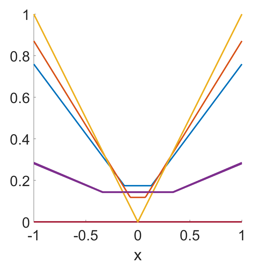
First, we use different initialization algorithms 1000 times and show the probability of born dying ReLU in Fig 1 by evaluating the networks only. It clearly shows that the LPS initialization has a much lower probability of a born dead neural network compared to He initialization. Second, we train different neural networks by these two initialization algorithms to see their effects on the training process. When the dying ReLU occurs, the training result becomes a flat line (x-axis) in 1D and a flat plane ( plane) in 2D. We call this the “collapse” case. But even for the non-collapse case, we cannot guarantee the loss goes to zero since the training algorithm may be trapped in a local minimum (See Fig. 2 for four non-collapse results which are randomly chosen from all non-collapse results of each function). Our algorithm focuses on the initialization part, not the training process. Therefore, we initialize times for each initialization algorithm (up to 8 re-initialization) and count how many times the training does not collapse which is shown in Table 1. It is obvious that the LPS initialization has a much lower chance with the dying ReLU during the training. Moreover, with only 6-7 re-initialization for and , the LPS initialization achieves the optimal performance which confirms the conclusion of Theorem 4.2.


| function | He initialization | LPS initialization | |||||||
| reinit=1 | reinit=2 | reinit=3 | reinit=4 | reinit=5 | reinit=6 | reinit=7 | reinit=8 | ||
| 4.5% | 9.5% | 18.8% | 28.1% | 37.4% | 40.2% | 37.0% | 40.4% | 38.7% | |
| 5.6% | 8.7% | 15.8% | 22.1% | 22.3% | 21.8% | 22.7% | 22.3% | 20.8% | |
| 3.2% | 12.4% | 29.2% | 43.6% | 58.0% | 74.1% | 81.9% | 88.2% | 92.1% | |
| 22.9% | 38.7% | 60.5% | 75.1% | 85.3% | 92.7% | 96.5% | 98.3% | 98.9% | |
5.2 Convolutional neural networks
We apply the LPS initialization to various benchmark models on public datasets. We use the cross-entropy as the loss function and the stochastic gradient descent (SGD) as the training algorithm.
5.2.1 LeNet networks on the MNIST dataset
First, we benchmark three different LeNet networks, LeNet-1, LeNet-4, and LeNet-5, on the MNIST dataset [24] to compare the LPS initialization with He initialization. Each initialization algorithm is used to generate 100 different initialization (up to three re-initialization for the LPS initialization). The error rates on the validation dataset for all the initialization algorithms are summarized in Table 2. The LPS initialization has lower error rates on both LeNet-4 and LeNet-5 and achieves a comparable error rate on LeNet-1 with He initialization. On LeNet-1, the LPS initialization has a larger deviation since it can compute all the local minima but some of them may have high generalization errors. In order to quantify the performances of different algorithms further, we define Good Local Minimum Percentage (GLMP) as the percentage of the validation accuracy greater than 99% in 100 initializations and show in Table 2. We find that the LPS initialization (with the optimal number of re-initialization) has a much better chance to find a good local minimum on all three models. Moreover, the LPS initialization achieves the optimal performance with only one re-initialization for LeNet-1 and LeNet-4 and with two re-initialization for LeNet-5.
| Network | He initialization | LPS initialization | ||||||
| reinit=1 | reinit=2 | reinit=3 | ||||||
| GLMP | error rate | GLMP | error rate | GLMP | error rate | GLMP | error rate | |
| LeNet-1 | 24% | 1.140.21% | 29% | 1.998.71% | 20% | 2.108.71% | 16% | 2.088.70% |
| LeNet-4 | 89% | 4.30%17.21% | 95% | 2.4512.31% | 89% | 6.8622.43% | 87% | 8.6125.16% |
| LeNet-5 | 84% | 13.9431.38% | 89% | 10.2927.54% | 93% | 6.7522.46% | 92% | 6.7622.46% |
5.2.2 VGG networks on the CIFAR-10 dataset
Secondly, we compare the LPS initialization with He initialization for different VGG networks, VGG9, VGG11, VGG13, and VGG16, on the CIFAR-10 dataset [25]. We run 10 initialization for each of them and show the comparisons in Table 3. All the error rates of the LPS initialization are comparable with He initialization but the lowest error rate (LER) of the LPS initialization is lower than He initialization. This confirms that the LPS initialization can find local minima in a larger solution landscape (with a larger deviation and lower LER) while He initialization focuses on a smaller solution landscape. The LPS initialization achieves the optimal performance of up to three re-initialization for all four VGG networks.
| Network | He initialization | LPS initialization | ||||||
| reinit=1 | reinit=2 | reinit=3 | ||||||
| LER | error rate | LER | error rate | LER | error rate | LER | error rate | |
| VGG9 | 5.95% | 6.090.10% | 5.89% | 6.020.06% | 5.82% | 6.060.13% | 5.84% | 6.110.16% |
| VGG11 | 7.34% | 7.620.17% | 7.51% | 7.89%0.21% | 7.42% | 7.820.20% | 7.17% | 7.950.36% |
| VGG13 | 5.84% | 5.960.06% | 5.73% | 6.01%0.16% | 5.84% | 22.8733.56% | 6.12% | 39.8840.92% |
| VGG16 | 6.25% | 6.39%0.10% | 6.15% | 14.7425.08% | 5.98% | 6.490.26% | 6.23% | 14.8425.05% |
5.2.3 ResNets on different datasets
Last, we validate the LPS initialization on different ResNets with public datasets. The ResNet architecture [26] does not have the vanishing gradient problem since skip connections act as gradient superhighways, allowing the gradient to flow unhindered. That’s the main reason why He initialization performs very well on the ResNets. We compare the LPS initialization with He initialization on different ResNets on CIFAR-10 and CIFAR-100 [25]. Results in Table 4 show that the LPS initialization achieves better error rates than He initialization. Fig. 3 shows that the LPS initialization has a comparable training performance to He initialization on the ImageNet dataset [27].
| Dataset | Network | He initialization | LPS initialization | ||||||
| reinit=1 | reinit=2 | reinit=3 | |||||||
| LER | error rate | LER | error rate | LER | error rate | LER | error rate | ||
| CIFAR-10 | ResNet-20 | 7.28% | 7.500.15% | 7.39% | 7.780.24% | 7.20% | 7.880.23% | 7.28% | 7.790.26% |
| ResNet-56 | 6.26% | 6.720.32% | 6.06% | 6.490.34% | 6.00% | 6.740.41% | 6.29% | 31.6638.18% | |
| ResNet-110 | 5.93% | 6.340.37% | 5.76% | 6.49%0.48% | 5.70% | 6.380.37% | 6.06% | 6.370.23% | |
| CIFAR-100 | ResNet-164 | 26.36% | 28.991.92% | 26.18% | 28.302.18% | 26.79% | 27.680.53% | 27.15% | 28.250.94% |


6 Conclusion
Weight initialization is crucial for efficiently training neural networks and therefore has become an active research area in machine learning. Current existing initialization algorithms are based on minimizing the variance of parameters between layers and lack consideration of the nonlinearity of neural networks which is the most essential part of the training. In this paper, we analyze the nonlinearity of neural networks from a nonlinear computation point of view and develop a novel initialization procedure based on the linear product structure of the neural network via approximating the ReLU activation function by polynomials. The LPS initialization can guarantee to find all the local minima based on the theory of numerical algebraic geometry and avoid the dying ReLU issue with the probability one from a theoretical perspective. Then we test this new initialization procedure on various benchmark networks and public datasets to show its feasibility and efficiency. We hope the LPS initialization complements current random initialization algorithms especially when the dying ReLU occurs. The theoretical analysis of the LPS initialization is for feedforward networks only and will be extended to the recurrent setting in the future. We will also further explore the LPS initialization to other activation functions and parameter normalization to improve efficiency.
Appendix
6.1 Proof of Theorem 2.1
Proof.
The Sobolev space is defined as
with
Then the estimate of the Legendre polynomial approximation [20] is : if , , we have
Since , we have the following approximation rate
| (15) |
Next we consider the optimal Legendre polynomial approximation for on in the norm. The Legendre’s differential equation is given by
| (16) |
for any . By multiplying and integrating from to on both sides, we have
| (17) |
Since
we simplify (17) as
| (18) |
where
| (19) |
Moreover,
| (20) |
then the coefficient of the optimal Legendre polynomial becomes
| (21) |
for any .
∎
6.2 Solving the polynomial system by homotopy continuation method
The quadratic and fourth degree approximated polynomials have the following explicit formulas
| (22) |
The comparison between the ReLU activation function and and is shown in Fig. 4.
We consider polynomial systems arising from fully connected neural networks to fit a 1D function .
One-hidden-layer neural network: We employ a one-hidden-layer ReLU network with width 2, namely,
| (23) |
where , and , and . By using the activation function, then becomes a quadratic polynomial
where
| (24) |
We consider a regression problem by using the ReLU neural network to fit and have the following polynomial system
By choosing a multi-homogenous start system [16], the homotopy method is used to obtain six solutions after tracking solution paths, namely,
| (33) |
Similarly, by solving the polynomial system with approximation, we obtain five solutions after tracking solution paths, namely,
| (34) |
Then we plug the solutions into the ReLU neural network and plot the in Fig. 4 which clear shows that we can recover by using the ReLU neural network via solving the polynomial system .

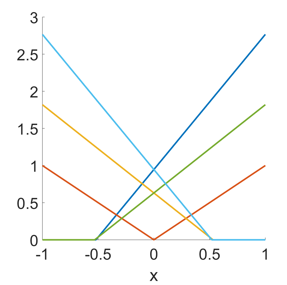
Multi-hidden-layer neural network: We employ -hidden-layer ReLU networks with width 2 to approximate with polynomial approximation. The numerical results of different multi-hidden-layer neural networks are summarized in Table 5 which clearly shows that the computational cost increase exceptionally as the layer goes deep. Therefore, the homotopy continuation method cannot be applied to solve large-scale neural networks directly.
Summary: Instead of solving the optimization problem, we solve a system of polynomial equations directly, namely, , where is the sample points on . Therefore, the homotopy continuation method can be used to solve the neural networks after approximating the activation function by polynomials and provides good initialization for the original neural network but cannot be applied to deep neural networks due to the high computational cost.
| # of hidden layers | # of solutions tracked | # of real solutions |
| 2 | 865 | 10 |
| 3 | 28,475 | 32 |
| 4 | 27,283,365 | 129 |
6.3 Proof of Theorem 4.2
Notations in the proof of Theorem 4.1
- •
Model without re-initialization: We rewrite the neural network model as
(35) with for all . are initialized randomly such as He’s initialization [5] or the LPS initialization without initializations. We denote for the element on -th row and -th column and for the -th element.
- •
Model with re-initialization: The neural network with one re-initialization (or times re-initialization as in the proof of Theorem 4.2) is denoted as
(36) with for all . Here are re-initialized with probability for these negative elements.
- •
We consider these next sets related to the initialization of neural network model:
In addition, we define the following sets:
where by Algorithm 1.
- •
The probability density function of the normal distribution, namely is
The Gauss error function: is defined as
(37)
The notations and definitions in the proof are summarized in the Appendix. Based on Lemma A.1 in [23], we have
| (38) |
Because for all , thus
| (39) |
Moreover, since for any in , we have the Bayes formula below:
| (40) |
where
Then we have
| (41) |
Therefore, our proof mainly focus on estimating , which has the following decomposition:
where the width of -th layer. Since
| (42) |
we obtain
| (43) |
For , by the definition of , there exists such that . Thus, for any , we have
| (44) | ||||
Computations of : Since , , and , we have
| (45) | ||||
where stands for the -th element of the vector . Because and are independent and identically distributed with the same normal distribution ( in Algorithm 1), thus
| (46) |
where . Then (45) becomes
| (47) | ||||
By denoting
| (48) |
we conclude that
| (49) |
Computations of : By the definition of , we have
| (50) |
Therefore,
| (51) | ||||
Due to the independence, we have the following inequality:
| (52) |
Because of the symmetry of the initialization and , we have .
Therefore
| (54) | ||||
which leads to
| (55) |
Finally, we get
| (56) | ||||
In summary, we have the final estimate by (41)
| (57) |
6.4 Proof of Theorem 4.2
Notations in the proof of Theorem 4.2 We have the following notations
- •
We denote .
- •
We define the following set
Since , we have
| (58) |
where
| (59) |
Since
| (60) |
where , with times re-samplings in times re-initializations, for any , we have
| (61) |
For , we know that occurs if and only if both the originally sampled and all the times re-sampled are negative, namely,
Moreover,
| (62) |
(61) becomes
| (63) |
6.5 Experimental details
6.5.1 Fully Connected Neural Networks
We compare the LPS initialization with He initialization on two fully connected neural networks to fit 1D and 2D functions. Fig 1 shows the probability of born dying ReLU for different initialization strategies by using the hyperparameters shown in Table 6 over 1000 initialization. The probability is computed by
By using the hyperparameters shown in Table 6, we train neural networks based on different initialization strategies to find “non-collapse" cases. More specifically, we employ the Adam optimization algorithm [28] with a learning rate of 0.001 with 4000 training steps. The training loss is based on the standard mean square error (MSE)
For different function, (), we set different collapse thresholds to distinguish “collapse" and “non-collapse" cases.
| Parameter | f1 | f2 | f3 | f4 |
| Number of sample points | 21 | 21 | 100 | 441 |
| Number of hidden layers | 10 | 10 | 10 | 20 |
| Size of hidden layers | 2 | 2 | 2 | 4 |
| Learning rate | ||||
| Collapse threshold | 0.09 | 0.2 | 0.2 | 0.2 |
| Optimizer | Adam | |||
| Dying threshold | ||||
| Training steps per run | ||||
| Number of runs | ||||
6.5.2 Convolutional neural networks
We use the hyperparameters shown in Table 7 to train LeNet networks on the MNIST dataset [24]. We compute the mean and standard deviation of error rates and Good Local Minimum Percentage (GLMP) which refers the percentage of the validation accuracy greater than 99% in 100 initialization.
| Parameter | Value |
| Number of epochs | 100 |
| Batch size | 64 |
| Initial learning rate | 0.05 |
| Learning rate schedule | Decrease by half every 30 epochs |
| Weight decay | |
| Optimizer | SGD with momentum = 0.9 |
| Bias initialization | False |
| Number of runs | 100 |
All the hyperparameters shown in Table 8 are used to train the VGG networks on the CIFAR-10 dataset [25].
| Parameter | Value |
| Data Augmentation | {RandomHorizontalFlip RandomCrop} |
| Batch normalization | True |
| Number of epochs | 250 |
| Batch size | 128 |
| Initial learning rate | 0.2 |
| Learning rate schedule | Decrease by half every 30 epochs |
| Weight decay | |
| Optimizer | SGD with momentum = 0.9 |
| Bias initialization | Both |
| Number of runs | 10 |
All the deep residual network architecture considered in our experiment are reported in [26]. We use the hyperparameters shown in Table 9 train the ResNets on CIFAR-10, CIFAR-100 [25], and ImageNet datasets [27].
| Parameter | CIFAR-10 CIFAR-100 | ImageNet |
| Data Augmentation | {RandomHorizontalFlip RandomCrop} | {RandomHorizontalFlip RandomResizedCrop} |
| Number of epochs | 250 | 90 |
| Batch size | 128 | {ResNet-50: 128, ResNet-34: 256} |
| Initial learning rate | 0.2 | 0.1 |
| Learning rate schedule | Decrease by half every 30 epochs | Decrease by every 30 epochs |
| Bias initialization | Both | False |
| Number of runs | 10 | 1 |
| Batch normalization | True | |
| Weight decay | ||
| Optimizer | SGD with momentum = 0.9 | |
References
- [1] Pascanu R, Mikolov T, Bengio Y. 2013 On the difficulty of training recurrent neural networks. In International conference on machine learning pp. 1310–1318.
- [2] Mishkin D, Matas J. 2015 All you need is a good init. arXiv preprint arXiv:1511.06422.
- [3] Nguyen D, Widrow B. 1990 Improving the learning speed of 2-layer neural networks by choosing initial values of the adaptive weights. In 1990 IJCNN International Joint Conference on Neural Networks pp. 21–26. IEEE.
- [4] Glorot X, Bengio Y. 2010 Understanding the difficulty of training deep feedforward neural networks. In Proceedings of the thirteenth international conference on artificial intelligence and statistics pp. 249–256.
- [5] He K, Zhang X, Ren S, Sun J. 2015 Delving deep into rectifiers: Surpassing human-level performance on imagenet classification. In Proceedings of the IEEE international conference on computer vision pp. 1026–1034.
- [6] Arpit D, Campos V, Bengio Y. 2019 How to initialize your network? robust initialization for weightnorm & resnets. In Advances in Neural Information Processing Systems pp. 10900–10909.
- [7] Kumar S. 2017 On weight initialization in deep neural networks. arXiv preprint arXiv:1704.08863.
- [8] Pennington J, Schoenholz S, Ganguli S. 2017 Resurrecting the sigmoid in deep learning through dynamical isometry: theory and practice. In Advances in neural information processing systems pp. 4785–4795.
- [9] Pennington J, Schoenholz S, Ganguli S. 2018 The emergence of spectral universality in deep networks. arXiv preprint arXiv:1802.09979.
- [10] Poole B, Lahiri S, Raghu M, Sohl-Dickstein J, Ganguli S. 2016 Exponential expressivity in deep neural networks through transient chaos. In Advances in neural information processing systems pp. 3360–3368.
- [11] Saxe A, McClelland J, Ganguli S. 2013 Exact solutions to the nonlinear dynamics of learning in deep linear neural networks. arXiv preprint arXiv:1312.6120.
- [12] Sussillo D, Abbott L. 2014 Random walk initialization for training very deep feedforward networks. arXiv preprint arXiv:1412.6558.
- [13] Chen Q, Hao W. 2019 A homotopy training algorithm for fully connected neural networks. Proceedings of the Royal Society A 475, 20190662.
- [14] Hao W. 2021 A gradient descent method for solving a system of nonlinear equations. Applied Mathematics Letters 112, 106739.
- [15] Hao W, Hu B, Sommese AJ. 2014 Numerical algebraic geometry and differential equations. In Future Vision and Trends on Shapes, Geometry and Algebra pp. 39–53. Springer.
- [16] Sommese A, Wampler C. 2005 The Numerical solution of systems of polynomials arising in engineering and science. World Scientific.
- [17] Mehta D, Chen T, Tang T, Hauenstein J. 2021 The loss surface of deep linear networks viewed through the algebraic geometry lens. IEEE Transactions on Pattern Analysis and Machine Intelligence.
- [18] Chon K, Cohen R. 1997 Linear and nonlinear ARMA model parameter estimation using an artificial neural network. IEEE transactions on biomedical engineering 44, 168–174.
- [19] Ma L, Khorasani K. 2005 Constructive feedforward neural networks using Hermite polynomial activation functions. IEEE Transactions on Neural Networks 16, 821–833.
- [20] Xiu D, Karniadakis G. 2002 The Wiener–Askey polynomial chaos for stochastic differential equations. SIAM journal on scientific computing 24, 619–644.
- [21] Hao W, Zheng C. 2020 An adaptive homotopy method for computing bifurcations of nonlinear parametric systems. Journal of Scientific Computing 82, 1–19.
- [22] Bates D, Hauenstein J, Sommese A, Wampler C. 2013 Numerically solving polynomial systems with Bertini vol. 25. SIAM.
- [23] Lu L, Shin Y, Su Y, Karniadakis G. 2019 Dying relu and initialization: Theory and numerical examples. arXiv preprint arXiv:1903.06733.
- [24] LeCun Y, Cortes C, Burges C THE MNIST DATABASE. http://yann.lecun.com/exdb/mnist/.
- [25] Krizhevsky A The CIFAR-10 and CIFAR-100 datasets. https://www.cs.toronto.edu/ kriz/cifar.html.
- [26] He K, Zhang X, Ren S, Sun J. 2016 Deep residual learning for image recognition. In Proceedings of the IEEE conference on computer vision and pattern recognition pp. 770–778.
- [27] Deng J, Dong W, Socher R, Li L, Li K, Li F. 2009 Imagenet: A large-scale hierarchical image database. In 2009 IEEE conference on computer vision and pattern recognition pp. 248–255. Ieee.
- [28] Kingma DP, Ba J. 2014 Adam: A method for stochastic optimization. arXiv preprint arXiv:1412.6980.