Extrapolated DIscontinuity Tracking for complex 2D shock interactions
Abstract
A new shock-tracking technique that avoids re-meshing the computational grid around the moving shock-front was recently proposed by the authors [1]. The method combines the unstructured shock-fitting [2] approach, developed in the last decade by some of the authors, with ideas coming from embedded boundary methods. In particular, second-order extrapolations based on Taylor series expansions are employed to trasfer the solution and retain high order of accuracy. This paper describes the basic idea behind the new method and further algorithmic improvements which make the extrapolated Discontinuity Tracking Technique () capable of dealing with complex shock-topologies featuring shock-shock and shock-wall interactions occuring in steady problems. This method paves the way to a new class of shock-tracking techniques truly independent on the mesh structure and flow solver. Various test-cases are included to prove the potential of the method, demonstrate the key features of the methodology, and thoroughly evaluate several technical aspects related to the extrapolation from/onto the shock, and their impact on accuracy, and conservation.
Keywords:
Shock-tracking , shock-fitting , unstructured grids , embedded boundary , shock interactions , Taylor expansions1 Introduction
The numerical models nowadays used in the simulation of compressible high-speed flows within the continuum framework can be cast into two main categories: shock-capturing (SC) and shock-fitting (SF). SC can be traced back to the 1950s paper by VonNeumann and Richtmyer [3] and lays its foundations in the mathematical theory of weak solutions [4]. The key ingredients of SC discretizations are very well known in the CFD community and need not to be recalled here. SF techniques, on the contrary, rely on a very different standpoint, which consists in identifying the shocks as lines within a two-dimensional (2D) flow-field (surfaces in 3D) and computing their motion, upstream and downstream states according to the Rankine-Hugoniot jump relations. Fitted-shocks made their first appearance in two NACA technical reports written by Emmons [5, 6] in the 1940s, but it is between the late 1960s and the end of the 1980s that the technique has been extensively developed by Gino Moretti and collaborators under the name “Shock-Fitting” and, starting in the early 1980s, by James Glimm and collaborators under the name “Front-Tracking”. Moretti’s SF techniques (both the “boundary” and “floating” variants) were designed for structured-grid solvers, the only kind of CFD codes in use at that time. The development of structured-grid SF codes turned out to be algorithmically fairly complex, especially when dealing with flows featuring shock-shock and shock-boundary interactions [7]. Algorithmic complexity contributed to make CFD practitioners “shy away from shock-fitting” [8] to embrace the myth of “one code for all flows” that has so much contributed to the popularity of SC discretizations.
Starting in the late 1980s, however, the CFD community has shown increasing interest towards unstructured meshes because of their ability to easily describe complex geometries and the possibility of locally changing the mesh size to adapt it to the local flow features. Taking advantage of the greater flexibility offered by unstructured meshes, Paciorri and Bonfiglioli [2] developed a new unstructured SF technique suitable for vertex-centered solvers operating with simplicial elements (triangles in 2D and tetrahedra in 3D). Their approach alleviated many of the algorithmic difficulties incurred by the SF techniques within the structured-grid setting. In recent years, the unstructured SF technique originally proposed in [2] has been further improved making it capable of dealing with multiple interacting discontinuities [9] and unsteady flows [10, 11] in 2D, as well as 3D flows [12], thus opening a new route for simulating compressible “shocked” flows. In particular, not only shocks and contact discontinuities are fitted, but also their interaction points, for example the triple point that arises in Mach reflections [13]. Most of the aforementioned developments have been included in an open-source platform [14] with the goal of fostering even more the interest in such methods.
Thanks to these new developments the interest in shock-fitting/tracking methods has seen a resurgence with the proposal of several implicit and explicit algorithms [15, 16, 17, 18, 19, 20, 21, 22, 23]. A limitation of this technique is that it heavily relies on the flexibility of triangular and tetrahedral grids to locally produce a fitted unstructured grid around the discontinuities.
The initial idea that motivated the present work comes from the similarity between the constraints
arising from SF, as conceived by Paciorri and Bonfiglioli in [2],
and those related to the construction of
boundary-fitted grids for simulating flows around complex geometries.
More precisely, the SF technique [2] requires that at each time-step the
computational grid is locally re-meshed to follow the moving shock-front.
This approach turns out to be best suited to vertex-centered CFD solvers,
but it can be problematic if a different type of data representation is used.
The approach, which has been described by the authors in [1]
and is further developed in this paper, allows to
overcome this limitation, because it avoids re-meshing by using ideas borrowed from
immersed and embedded boundary methods developed
to allow a flexible management of complex geometries. These two approaches rely on different philosophies, however.
Immersed methods are based on an extension of the flow equations outside the physical domain
(typically within solid bodies). This extension is formulated using some smooth
approximation of the Dirac delta function to localize the
boundary, as well as to impose the boundary condition. These methods are relatively old, and based on the original
ideas of Peskin [24]. Finite element and unstructured mesh extensions for elliptic PDEs
as well as for incompressible, and compressible flows have been discussed in [25, 26, 27].
Embedded methods, on the other hand, solve the PDEs only in the physical domain, while
replacing the exact boundary with some less accurate approximation, combined
with some weak enforcement of the boundary condition. There is a certain number of techniques
to perform this task, which go from the combination of XFEM-type methods with
penalization or Nitsche’s type approaches [28],
to several types of cut finite element methods with improved stability [29, 30], to
approximate domain methods such as the well known ghost-fluid method [31, 32],
and the more recent shifted boundary method (SBM) [33, 34].
As in the latter, we impose modified conditions on surrogate shock-manifolds, acting as boundaries
between the shock-upstream and shock-downstream regions. The values of the flow variables imposed
on these surrogate boundaries are extrapolated from the tracked shock-front, accounting for
the non-linear jump and wave propagation conditions, as done in the unstructured SF approach of [2].
As in shock-fitting and front-tracking methods [35], the shock-front is discretized
by an independent lower-dimensional mesh, and its position, as well as
the position of the two surrogate boundaries, are themselves part of the computational result.
In this paper, we focus on the new features coded in the algorithm to enable the computation of shock-shock and shock-wall interactions. In particular, when several discontinuities are mutually interacting, or interact with a solid boundary, the following issues must be addressed:
- 1.
identification of the various sub-domains obtained when the discontinuities cut through the computational domain;
- 2.
calculation of the velocity of those points where different discontinuities mutually interact (for example the triple point in a Mach reflection) or reach the boundary;
- 3.
the algorithm used to transfer the dependent variables between the shock-front and the surrogate boundaries must be applicable also when the shape of the surrogate boundaries becomes very complex, which typically occurs in the neighborhood of an interaction.
2 Generalities
We consider the numerical approximation of solutions of the steady limit of the Euler equations reading:
| (1) |
with conserved variables and fluxes given by:
| (2) |
having denoted by the mass density, by the velocity, by the pressure, and with the specific total energy, being the specific internal energy. Finally, the total specific enthalpy is , with the specific enthalpy. For simplicity in this paper we work with the classical perfect gas equation of state:
| (3) |
with the constant (for a perfect gas) ratio of specific heats. However, note that the method discussed allows in principle to handle any other type of gas, see e.g. [36].
In all applications involving high-speed flows, solutions of (1) are only piecewise continuous. In space dimensions, discontinuities are represented by manifolds governed by the well known Rankine-Hugoniot jump conditions reading:
| (4) |
having denoted by the local unit vector normal to the shock, by the corresponding jump of a quantity across the discontinuity,
and with the normal component of the shock speed.
As discussed in the introduction, the method proposed exploits ideas from two different approaches:
the unstructured shock-fitting method [2] and subsequent works [9, 12, 10]; the shifted boundary method by [33] and subsequent works [34, 37].
Although the paper focuses on triangle based nodal solvers, the method proposed is also applicable to structured and unstructured cell-centered solvers [38].
3 Extrapolated DIscontinuity Tracking ()
3.1 Generalities
To illustrate the algorithmic features of the method, let us consider a two-dimensional domain and a discontinuity front crossing the domain at a given time . As shown in Fig. 1a, the front is described using a collection of edges whose endpoints are marked by squares. Throughout the paper these two entities will be referred to as front-edges or discontinuity-edges, and front-points or discontinuity-points respectively, and together they constitute what will be referred to as front-mesh or discontinuity-mesh. The computational domain itself is discretized by means of a background mesh. As already said, we consider here solvers based on a nodal variable arrangement on triangular grids, but the extrapolation proposed readily applies to cell-centered solvers. Figure 1a clearly shows that the position of the discontinuity-points is completely independent of the location of the grid-points of the background mesh. Regardless of the method used to solve the Euler equations on the background mesh, the representation of the flow variables across the discontinuity is discontinuous. In our case, two values of the flow variables are stored in each front-point. Other arrangements (edge based for example) are of course possible. The flow solvers considered here are based on a continuous nodal approximation, which amounts to store one solution value at each grid-point of the background mesh. As already said, this is not essential for the method developed.
Assume that at time t the solution is known at all grid- and discontinuity-points. The computation of the subsequent time level t+t using the method can be split into several steps that will be described in detail in the following sub-sections.
3.2 Geometrical setting
The first step consists in flagging the triangles crossed by the front. As shown on Fig. 1b, this leads to the creation of a cavity of flagged elements enclosing the discontinuity. Here, in contrast to the unstructured technique proposed in [2], or to more classical methods such as the boundary shock fitting [39], the mesh within or in proximity of this cavity is not modified to be conformal with the discontinuity. This cavity separates two sub-domains, and allows to define two surrogate boundaries, which are the intersections between the boundaries of the sub-domains and the boundaries of the front cavity. The mesh of the sub-domains separated by the front cavities will be referred to as the computational mesh. The computational mesh is identical to the background mesh, except for the removal of the flagged elements enclosing the discontinuity. In the simplest setting of a single discontinuity, the upstream and downstream surrogate boundaries, drawn using red lines in Fig. 1b, will be called and . In the following we also refer to them as surrogate-discontinuities. The discontinuity-boundary, representing the actual front position, will be referred to as and its upstream and downstream sides as and , respectively. Contrary to and , and are superimposed and, of course, coincide with .
Compared to its original version [1], the current algorithm is capable of dealing with several discontinuity-fronts which implies that the computational domain is split into several, disjoint, sub-domains.
To apply the Rankine-Hugoniot jump relations (4) within each pair of discontinuity-points, we need to define the tangent and normal directions, and , in correspondence of each of these points. The computation of these vectors is carried out using finite-difference formulae which involve the coordinates of the front-point itself and those of the neighboring front-points that belong to its range of influence. Specifically, centred finite difference formulae will be used when the downstream state is subsonic whereas upwind formulae are employed whenever the downstream state is supersonic. Further details are given in [1, 40]. The unit vector is conventionally assumed to be directed from the high entropy (downstream) side towards the low entropy (upstream) side of the discontinuity, see Fig. 2. It is also convenient to express the components of the velocity vector in the reference frame which is locally attached to the discontinuity:
| (5) |
3.3 Definition of the sub-domains
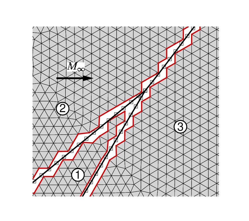
In principle the flow may evolve different fronts, which need to be handled numerically. The identification of these discontinuities is in itself a challenging problem (see e.g. [41, 42] and references therein), which is out of the scopes of this work. Here we assume to be given in advance a set of discontinuities, as well as their topology and nature (shocks and/or contact discontinuities), and the set of numbered sub-domains separated by the discontinuities. We also start from a brute set of the ensemble of all points and edges of the surrogate discontinuities, which we denote by . We process this ensemble as follows:
- 1.
associate to each point in the index of the closest discontinuity (distance measured by orthogonal projection);
- 2.
associate to each point in the Upstream/Downstream flag based on its position w.r.t. the orientation of the front normals;
- 3.
for each discontinuity assemble the corresponding arrays of upstream and downstream surrogate boundaries (edge collection) as better shown in Fig. 2;
- 4.
build a pointer providing the explicit mapping between actual and surrogate discontinuities.
The connectivity obtained allows to move easily from one surrogate discontinuity to the corresponding front-mesh, or to the other surrogate corresponding to the same discontinuity (e.g. move between the upstream and downstream surrogates and of the two shocks of Fig. 2), as well as between different surrogates bounding the same sub-domain (e.g. from to in Fig. 2).

3.4 Solution update using the CFD solver
The solution is updated to time level t+t using a shock-capturing code.
The flow computations are performed on the non-communicating sub-domains separated by the front cavity,
and including the surrogate discontinuities and as boundaries
(see Fig. 3).
As we will see in the next section, the boundary conditions imposed on the surrogate discontinuities are defined
starting from the values of the flow variables on and which, as already said, are
in general different, because is a discontinuity.
Concerning the solver used in this paper, it is based on a Residual Distribution (RD) method evolving in time
approximations of the values of the flow variables in grid-points. The method has several appealing characteristics,
including the possibility of defining genuine multidimensional upwind strategies for Euler flows, by means of a wave decoupling
exploiting appropriately preconditioned forms of the equations [43].
By combining ideas from both the stabilized finite element and finite volume methods, these schemes allow to achieve
second order of accuracy and monotonicity preservation with a compact stencil of nearest neighbors.
The interested reader can refer to [44, 45] and references therein for an in-depth review of this family of methods,
as well as to [43, 46] and references therein for some specific choices of the implementation used here.
3.5 Surrogate discontinuity conditions update
The flow solver provides updated nodal values at all grid-points of the computational mesh
at time level t+t.
When dealing with shock waves, the shock-upstream surrogate boundary, behaves like
a supersonic outflow and, therefore, no boundary conditions should
be applied. However, along the
shock-downstream surrogate
the flow is subsonic in the shock-normal direction and in principle only the
characteristic variable11
1
Hereafter, characteristic variables shall also be referred to as Riemann variables. conveyed by the slow acoustic wave has been correctly updated,
while boundary conditions for the remaining ones
(the fast acoustic, entropy and vorticity waves) should be imposed. The situation is similar on both sides of a contact discontinuity.
Updating correctly the interface conditions across the embedded discontinuity is very delicate, and it is the key of the method proposed. It involves several steps, which are detailed hereafter.
3.5.1 Computational mesh to discontinuity mesh transfer
The transfer of the flow data from the computational mesh to the front-mesh is necessary before imposing the interface conditions. In this work we use a CFD solver strongly relying on the use of Roe’s parameter vector [47, 48] as the dependent variable, so the transfer is also done in terms of . This is evidently not a necessary choice, and any other choice of state vector is acceptable. This first transfer is required to update the flow variables along and . Following [37, 1], this is achieved by first defining a map:
| (6) |
where, as shown in Fig. 4, the point belonging to the computational mesh is the projection in the direction of the front-normal of a front-point of the front-mesh. Then we use a forward Taylor series expansion to express the data along the discontinuity in terms of the values of the flow variables and of their derivatives on the computational mesh. A first-order transfer reads:
| (7) |
while a second order extrapolation is written as:
| (8) |
With the exception of few methods based on a approximation (see e.g. [49]),
in general, the gradients of the flow variables are undefined at mesh-points.
To avoid handling specific singular cases, we have
implemented (8) using interpolated reconstructed nodal gradients.
Note that, in order to achieve an overall second order of accuracy in the calculation
of , the approximation of the gradient in Eq. (8) only needs to be consistent, i.e. at least first-order-accurate.
In practice we proceed as shown in Fig. 4. When moving from the computational mesh to (see Fig. 4a) a front-point is mapped to a point . The values of the dependent variables and of their gradients in are interpolated from the neighbors and :
| (9) |
where is either or , and and are the weights,
equal to the normalized distances between and grid-points and .
The evaluation of the gradient in the grid-points of the surrogate boundaries
may be performed using different approaches, as reported in § 3.7.
Once the value of and in
point has
been computed using Eq. (9),
in is computed by means of Eq. (8),
having set and .
When moving from the computational mesh to the
procedure is identical: the front-point is updated using its mapped point (see Fig. 4b). Values of the relevant quantities are again linearly interpolated, and
is computed by means of Eq. (8), having set and .
3.5.2 Riemann variables and jump conditions enforcement
The solution updated by the flow solver and extrapolated to the discontinuity mesh does not take into account the coupling between the different sub-domains. This coupling is done here based on the Rankine-Hugoniot jump relations. On the upstream side of a shock wave all the Riemann variables are transported into the shock, so the data extrapolated from the computational mesh on this side is assumed to be correct. On the shock-downstream side, however, this holds true only for the Riemann variable associated with the slow acoustic wave that moves towards the shock (the subscript D denotes values along ):
| (10) |
We need to provide relations to compute along the values of the Riemann variables corresponding to the fast acoustic wave, as well as to the entropy and vorticity waves. These relations are supplied by the Ranking-Hugoniot jump conditions which, for a perfect gas, can be recast as:
| (11) |
with the shock speed. The algebraic non-linear system made up of
Eqs. (10) and (11) allows to compute the five unknowns given
the known upstream state
and the slow acoustic Riemann variable .
For a contact discontinuity, we use as input the following set of Riemann variables, which we assume to be correctly updated in the computational mesh:
| (12) |
Note that when dealing with a contact discontinuity the situation is essentially symmetric and the jump relations simplify somewhat, and can be shown to reduce to:
| (13) |
The algebraic non-linear system made up of Eqs. (12) and (13) allows to compute the nine unknowns
, given the six
Riemann variables
on the two sides of the discontinuity and the jump relations (13).
For both shocks and contact discontinuities, a non-linear system of algebraic equations
needs to be solved in each discontinuity-point. This is done
using the Newton-Raphson root-finding algorithm,
thus providing the correct states and at time level t+t.
Whenever two or more discontinuities interact special care is required for the front-points belonging to different discontinuities.
The numerical treatment of these points is done in a case by case manner and detailed in the sections related to the specific tests in § 5.
3.5.3 Discontinuity mesh to computational mesh transfer
Once the value of the unknowns have been corrected along the discontinuity mesh to account for the jump conditions, the corrected values need to be transferred back to the surrogate discontinuities. To do this, we proceed in a similar manner as before by writing:
| (14) |
Note that there is a substantial difference in the direction in which the Taylor expansion is performed which is now a backward expansion from the arrival point (the surrogate discontinuity) to the point where the data is available (the discontinuity mesh). As in the previous case, several choices are possible to evaluate the gradient involved in this transfer. We shall focus on this in § 3.7. In the first-order accurate case, Eq. (14) simplifies to:
| (15) |
Finally note that for shock-waves only grid-points on need to be updated.
3.6 Front displacement and nodal re-initialization
The new position of the front at time level t+t is computed by displacing all discontinuity-points using the following first-order-accurate (in time) formula:
| (16) |
where denotes the geometrical location of the shock-points, and
may represent either or .
The use of a first-order-accurate temporal integration formula has no impact as long as steady flows are of interest.
For unsteady flows, second-order-accurate time integration formulae should be used, as done for example in [10, 11].
Since the discontinuity can freely float over the background triangulation, it may happen that it crosses the surrogate boundaries. This situation has been sketched in Fig. 5, where grid-point has been overtaken by the moving front. Whenever this happens, the flow state within grid-point has to be changed accordingly.
In particular, the flow variables in these points are re-computed through an interpolation. To evaluate whether a grid-point has been overtaken or not by the discontinuity a simple approach has been implemented. Since points always upstream, the sign of the following scalar product allows us to distinguish the grid-points located upstream from those located downstream.
| (17) |
where and are, respectively, the coordinates of a grid-point and its projection over the closest front-edge and is the normal vector computed in the closest front-point to . If changes sign when the front moves, this means that grid-point has been overtaken and its state has to be updated.
3.7 Evaluation of the nodal gradients
The technique used to extrapolate the flow variables back and forth between the surrogate discontinuities and the discontinuity mesh involves
the knowledge of nodal gradients which need to be reconstructed. The solvers used in this work are based on collocated nodal methods, so we will discuss
the recovery of the nodal gradients in this specific case. The generalization to other cases is of course possible,
but left out of this work.
As for the enforcement of the jump conditions we distinguish two main cases. For a shock wave, in the upstream domain we already said that all characteristic information runs into the shock. For this situation, it seems natural to evaluate the nodal gradients along the surrogate discontinuity based on the data pre-computed by the flow solver within the upstream domain. To this end we have tested two gradient recovery strategies:
- 1.
a Green-Gauss (GG) gradient reconstruction, essentially boiling down to an area weighted average of the gradients in the cells surrounding a grid-point;
- 2.
an area-weighted version of Zienkiewicz-Zhu’s patch super-convergent method (ZZ) [50].
Explicit formulas for both methods are provided in A.
Within the region downstream of a shock, as well as for contact discontinuities, as discussed in the previous sections, the data computed by the flow solver must be corrected to account for the jump conditions. This fact has led us in the past to include the corrected data in the evaluation of the nodal gradients in these cases [1]. In the aforementioned reference, which did not account for discontinuity interactions, the gradient term of Eq. (14) is replaced with the cell-wise gradient of an auxiliary triangle (marked using a dashed line in Fig. 6) containing the surrogate grid-point to be updated (grid-point in Fig. 6), and defined by a point on the discontinuity-mesh (point in Fig. 6), and two grid-points of the computational mesh, not belonging to the surrogate discontinuity. However, when interactions are present, singular topological situations may arise in which this approach cannot be used. For example, for region in Fig. 6, a long strip of one row of elements is trapped within two discontinuities and the interaction point. For the grid-points along the boundary of this strip there are no neighboring inner grid-points to construct the auxiliary triangle. Several other gradient-reconstruction formulations have also been tested. The simplest involves using a one-sided recovered gradient not accounting for the Rankine-Hugoniot correction. The latter not only turned out to be very useful for computing interacting discontinuities, but much simpler, especially in view of possible extensions to three space dimensions. In the following, we will refer to the method of [1] as , while (GG reconstruction), and (ZZ reconstruction) will denote the extrapolated discontinuity tracking obtained using one sided reconstructions. Finally, (first order) refers to simulations run with a second-order-accurate discretization of the governing PDEs, but only first-order accurate data transfer between the surrogate and actual discontinuities, i.e. by using Eqs. (7) and (15).
4 Remarks on conservation
We make a small detour to discuss the issue of conservation. A first important remark is that the notion of conservation is essential when considering the approximation of shocks. Failing to properly account for conservation of mass, momentum, and energy would lead to a wrong approximation of these features, both in terms of position and strength. In smooth regions, as well as across contact discontinuities, the use of non-conservative approaches is less critical, and in some cases even advantageous (e.g. [51, 52, 44, 53]).
It is also important to realize that the definition of discrete conservation is associated to the identification of both a geometrical cell over which conservation is expressed, and a numerical flux expressing local conservation. The interested reader can refer to [45, 54] for a discussion. Typically, global conservation over the domain is thus expressed as
| (18) |
with the numerical flux associated to the boundary conditions.
Now note that, even for exact quadrature, the numerical flux is not equal to the physical one ,
and the difference between the two is in general of the order of the truncation error of the discretization. So conservation is still
verified within some numerical approximation.
The situation is similar for the embedded approach proposed here, for which, despite the exact imposition of the jump conditions across discontinuities, conservation can only be measured within the truncation of the extrapolation method. To be more precise, let us focus on the configuration of Fig. 7. In the figure, the domains on the right of is the upstream domain, while the domain on the left of is the downstream one. The flow is assumed to go from the right to the left. A discontinuity is placed in the middle of the domain. We have denoted by and the upstream and downstream sides of the discontinuity. The discretization of all the domains, including the upstream/downstream boundaries and the discontinuity, is shown in the figure. In particular, as already discussed, unlike in the unstructured shock-fitting method [2], for the method the shock-edges are no longer part of the computational mesh. In the region between the shock mesh and the computational mesh, the conservation law is then replaced by the extrapolation procedure, which is the main source of loss of conservation. Note however, that this loss only occurs in the smooth parts of the flow. In particular, denoting by the region enclosed between and , given a smooth exact solution of the Euler equations we can write easily the upstream consistency estimate
Where is the Roe’s parameter vector evaluated for the exact solution. Formally replacing the nodal values of the solution with those of the exact one, we obtain the consistency estimate . Using the exact same arguments, we can write the estimate for the loss of conservation in the downstream region enclosed between and .
Let us now set and . By construction of the method proposed here, the jump condition is exactly satisfied. This allows readily to write the global consistency estimate on conservation (cf. 7 for the notation)
| (19) |
reducing to
| (20) |
whenever the out/inflow on the top/bottom boundaries is zero. So the conservation error is solely controlled from the accuracy of the extrapolation formula. This means that first or second order is obtained in terms of conservation, and thus in terms of position and magnitude of the discontinuities, depending on whether the gradient correction is included or not. This will be verified in practice in the numerical results section. Note that this behaviour is better than what any fully conservative capturing method can provide, and can of course be further improved by enhancing the extrapolation accuracy.
5 Numerical Results
To illustrate the capabilities of our method, we provide here examples representative of several types of interactions which can occur in gas-dynamics. The solutions obtained with the extrapolated tracking method will be compared to i) full-fledged computations, ii) hybrid simulations in which only some of the discontinuities are explicitly tracked while the others are captured, and iii) solutions obtained with the standard shock-capturing method. To evaluate the gradient recovery strategies, a grid-convergence analysis is presented for two test-cases (transonic source flow and blunt body problem) to asses quantitative differences between the approach described in [1] and the more flexible ones proposed here to deal with interactions.
5.1 Transonic source flow
This test-case is very useful because of the availability of the analytical solution, which allows to perform grid-convergence studies [1, 55, 56]. Assuming that the analytical velocity field has a purely radial velocity component, it may be easily verified that the two-dimensional, compressible Euler equations, written in a polar coordinate system, become identical to those governing a compressible quasi-one-dimensional flow with a nozzle area variation linear w.r.t. the radial distance from the pole of the reference frame.


The computational domain consists in the annulus sketched in Fig. 8a: the ratio between the radii of the outer and inner circles () has been set equal to / = 2. A transonic (shocked) flow has been simulated by imposing a supersonic inlet flow at on the inner circle and a ratio between the outlet static and inlet total pressures such that the shock forms at / = 1.5. The Delaunay mesh shown in Fig. 8b, which contains 6,916 grid-points and 13,456 triangles, has been generated using the gmsh mesh generator [57] in such a way that no systematic alignment occurs between the edges of the triangulation and the circular iso-contour lines of the analytical solution. By doing so, the discrete problem is made truly two-dimensional. The sequence of nested triangulations that have been employed for and all computations are summarized in Tab. 1 for both the background and the computational grids.
| Background grid | Both grids | Computational grid | |||
|---|---|---|---|---|---|
| Grid level | Grid-points | Triangles | Grid-points | Triangles | |
| 0 | 1,369 | 2,548 | 0.5286E-01 | 1,369 | 2,328 |
| 1 | 5,286 | 10,192 | 0.2641E-01 | 5,286 | 9,788 |
| 2 | 20,764 | 40,768 | 0.1320E-01 | 20,764 | 39,968 |
| 3 | 82,296 | 163,072 | 0.6602E-02 | 82,296 | 161,454 |
The discretization error for a mesh of size , , is defined as the difference between the numerical solution, , and the analytical one, :
| (21) |
The availability of the exact solution allows to compute the discretization error locally using Eq. (21) or, globally, by computing the norms of the discretization error over the entire computational domain using Eq. (22):
| (22) |
Herein, the norm has been employed and computed using Gaussian quadrature rules.
Different versions of the extrapolated shock/discontinuity tracking method will be compared to
computations by doing a thorough grid-convergence analysis.
Results obtained from the aforementioned approaches
have been separately displayed in the grid-convergence plots for the shock-upstream (supersonic) and shock-downstream (subsonic)
regions, i.e. and . In all convergence plots the errors are computed in terms of the parameter vector .
Firstly, the global errors obtained on the shock-upstream side of the domain have been displayed to corroborate the fact that, for the supersonic region, the results obtained with all methods are almost identical. Indeed, Fig. 9 shows that, on the shock-upstream side, all approaches are able to retain the formal order of accuracy of the method.
Instead, when looking at the results shown in Fig. 10,
which shows the global errors within the subsonic region,
the situation is considerably different.
An almost asymptotic convergence is observed
for all second order versions of the extrapolated tracking method (, and ).
Instead, for , the convergence rate drops to one, and even less for the coarsest meshes.
and solutions are almost indistinguishable,
with global errors that favor more the first approach,
probably due to the use of flow data explicitly accounting for the jump conditions also in the extrapolation. The
is still comparable having a trend in the middle between the two.
Although the differences are not remarkable, using a more accurate reconstruction seems to have some effect on the magnitude of the error. The improvement is however so small that the
can be safely replaced by either or . This also shows that our basic idea can be coupled to different extrapolation methods, and others, possibly improved ones, could be suggested in the future.
As expected, performs as the others in the supersonic side of the domain showing a second-order trend.
However in the subsonic side, due to the first order extrapolations carried out at the shock,
its trend follows the first order slope curve, because it does not include the nodal gradients
in the extrapolation.
Figure 12 points out the flux balance computed on the two surrogate boundaries and showing that convergence
trends strictly depends on the order of the extrapolation.
It is indeed shown that first (second) order behaviour is displayed for first (second) order extrapolations, confirming the arguments of § 4.
Finally, Fig. 11, which plots the local discretization error against the radial distance , clearly reveals the huge reduction of the numerical errors that the various approaches provide w.r.t. . The green line in Fig. 11 represents the actual position where the shock occurs (). As already verified in Fig. 9, the error computed with either or any of the versions within the shock-upstream region is almost the same.


Iso-contour lines of the fourth component of computed on grid level 2 are displayed in Fig. 13: the solution is shown in Fig. 13a, whereas Fig. 13b shows the results of two different calculations. More precisely, the second-order-accurate result is displayed in the upper half of Fig. 13b and is shown in the lower half of the same frame. When mutually comparing the three different calculations, it can be seen that both the and calculations are affected by severe oscillations downstream of the shock, which completely disappear when using . Even though the solution looks slightly better than the one, Fig. 10 confirms that cannot be better than first-order accurate behind the shock.


5.2 Hypersonic flow past a blunt body
We consider now a hypersonic ( 20) flow past the forebody of a circular cylinder. Compared to the previous test-case, this flow is a comprehensive test-bed for the algorithm, because the entire shock-polar is swept whilst moving along the bow shock which forms ahead of the blunt body. Moreover, as shown in Fig. 14a, the flow-field is much more complex than that examined in § 5.1, due to the presence of a stagnation region within a subsonic pocket, as well as a smooth re-acceleration of the flow to supersonic conditions along the body.


Even though no analytical solution is available for the entire flow-field, we know that total enthalpy, , is preserved along streamlines at steady state. For a constant profile of ahead of the shock, this leads to an exact solution featuring a homogeneous total enthalpy field, thus the condition can be used to study the convergence behaviour of the various combinations of numerical schemes and shock-modeling options. Starting from a coarse mesh (shown in Fig. 14b) obtained with the delaundo frontal/Delaunay mesh generator [58, 59], we created three levels of nested refined meshes with characteristics summarized in Table 2 for both the background and computational grids.
| Background grid | Both grids | Computational grid | |||
|---|---|---|---|---|---|
| Grid level | Grid-points | Triangles | Grid-points | Triangles | |
| 0 | 351 | 610 | 0.16 | 351 | 535 |
| 1 | 1,311 | 2,440 | 0.08 | 1,311 | 2,292 |
| 2 | 5,061 | 9,760 | 0.04 | 5,061 | 9,460 |
| 3 | 19,881 | 39,040 | 0.02 | 19,881 | 38,439 |
The different extrapolated tracking methods discussed in the previous sections are expected to provide orders of convergence similar to those observed for the source flow of § 5.1, as well as smooth and clean results with very low numerical perturbations, even on the coarsest grids; this latter aspect is illustrated in Fig. 15, where the pressure iso-contour lines computed using on the level 0 (coarsest) and level 3 (finest) grids are mutually compared.
Figure 16a shows the grid-convergence analysis pointing out again that the different extrapolation techniques provide error levels relatively close, and a second order slope,
while the captured result converges with a less than first order rate, and errors of one or two orders of magnitude larger.
The patch super-convergent gradient recovery () provides a better result for this case.
Figure 16b shows the effect of a second order extrapolation, , on the flux balance within the cavity for this test-case.
As discussed in § 4 we recover the error associated to the second order extrapolation.
Similar results for other second order extrapolations are straightforward to obtain and therefore not included in Fig. 16b.
Figure 17 shows the total-enthalpy discretization error over the entire computational domain for the two solutions obtained with and and two different grid-levels: the coarsest and the finest. The maximum value of the error is also explicitly given in each of the four frames. While confirming the lower error levels on the coarse mesh, and the rapid error convergence obtained with second-order shock-tracking, the four frames of Fig. 17 allow to visually highlight the substantial difference in error generation. Indeed, in both captured solutions (Fig. 17a and 17c), the largest error is generated along the shock. Conversely, for the two calculations the numerical error is essentially connected with the wall boundary condition, and undoubtedly related to the entropy generated at the stagnation point and advected downstream. The solution is virtually identical and not discussed for brevity.
As a final note, we remark that total enthalpy is a conserved variable if and only if the time derivative in Eq. (1) vanishes. This means that the convergence to steady state plays a major role in allowing to correctly measure the decay rate of the discretization error. Convergence to steady-state is an important aspect of this type of methods, which is why we also report on Fig. 18 the iterative convergence of the algorithm when starting from a captured solution. In all our calculations we have set as a stopping criterion a threshold on the norm of the shock speed of . As Fig. 18 shows, this level is reached quite monotonically in all the computations. This despite the shock crossing some nodes during the iterations, which produces a change in topology of the surrogate discontinuities and of the computational domain which can be seen in some of the peaks appearing locally in the iterative convergence plots. Similar convergence curves are often hard to obtain with non-linear shock capturing methods.


5.3 Interaction between two shocks of the same family
The present and subsequent test-cases address the interaction among different discontinuities, a kind of flow-topology which had not been addressed in the first journal appearance [1] of the algorithm and thus represent one of the key novelties of this study.

We consider here the interaction between two oblique shocks
colliding and giving rise to a five-waves interaction. As shown in the sketch of Fig. 19,
the two incident shocks (IS1 and IS2) of the same family
interact in a quadruple point, referred to as QP in the figure, generating three reflected discontinuities: a strong reflected shock
(RS1), with jumps of magnitude larger
than the two incident ones; a contact discontinuity (CD); a weak reflected shock (RS2), with jumps so small that it could
be considered as a Mach wave.
More in general, depending on the free-stream Mach number and the flow deflection angles
caused by the incident shocks, RS2 can be either a weak expansion or compression wave.
With reference to Fig. 19, in this case the free-stream Mach number and the flow deflection
angles are: , and
which can be shown to lead to states 4 and 5 characterized by ,
, and .
For this choice of parameters, RS2 is so weak that
we decided not to track this wave since its resolution has negligible overall effect on the flow.
Simulations of the interaction have been performed using a Delaunay triangulation containing 7,921 nodes and 15,514 triangles. As before, the same mesh is used to perform the simulation and as a background grid for the computations. Results with the are virtually identical to the latter, and not discussed.


As mentioned in § 3.5.2, the interaction points need to be modelled explicitly on a case by case basis. If only some of the discontinuities meeting at the interaction point are tracked, the only possibility is to solve independent algebraic problems arising from the jump conditions for each discontinuity, and use some approximate formula for QP. For the type of interaction considered here, we have used the following relation to compute the velocity of the interaction point QP:
| (23) |
where is the vector tangential to IS1 (see Fig.19a). Equation (23) is similar, but not identical, to the formula proposed in [19] for the same purpose.
We compare in Fig. 20 three sets of results: i) a fully captured solution (top row of Fig. 20); ii) a hybrid solution in which CD is captured, and all the shocks (IS1, IS2 and RS1) are tracked (central row of Fig. 20); iii) a fully tracked result (bottom row of Fig. 20) where also CD is fitted. First of all, this result shows that it is possible to track several discontinuities and capture others, all involved in the same interaction. Compared to the fully captured solution, this hybrid simulation with captured CD provides a much cleaner entropy field, as seen comparing the top and central rows of frames in Fig. 20. However, we can also see a small anomaly due to the capturing of the CD, which is still observable in part of the flow downstream of the reflected shock RS1: see the close up of Fig 20d. These spurious disturbances are removed by adding the contact discontinuity to the set of discontinuities to be tracked by the algorithm, as visible on the bottom row of results of Fig. 20. Note that despite its apparent simplicity, the results obtained are surprisingly good as this is a difficult simulation. Indeed, on a mesh as coarse as the one used here, the elements crossed by the discontinuity generate a relatively large cavity around the interaction point. This is clearly visible for example in Fig 20f. The extrapolation strategy proposed allows to handle this delicate geometrical situation.
5.4 Shock-wall interaction: Mach reflection

An oblique shock that impinges on a straight wall gives rise to either a regular or a Mach
reflection, depending on the combination of free-stream Mach number, , and flow deflection
angle, , that the free-stream flow undergoes while passing through the oblique shock (hereafter also referred to as the incident shock).
Whenever is
larger than the maximum deflection that the supersonic stream behind the
incident shock can sustain, a Mach reflection takes place.
As sketched in Fig. 21,
a Mach reflection consists in a fairly complex three-shocks system
(the incident shock, IS, the reflected shock, RS, and the
Mach stem, MS) interacting in the triple point, TP, from which a contact discontinuity, CD, also arises.
Note that differently from the test-case addressed in § 5.3,
here not all the regions surrounding TP involve uniform flow.
Moreover, CD presents a slight angle, which makes it in general not mesh-aligned.


For the chosen setting, and , we consider four different types of simulations:
- 1.
fully captured;
- 2.
an extrapolated shock-tracking setting in which the Mach stem (MS) and the reflected shock (RS) are tracked as a single discontinuity;
- 3.
a hybrid setting in which only the shocks are tracked, but CD is captured;
- 4.
full-fledged discontinuity-tracking for all shocks plus the CD.
Note that no modelling of the triple point TP is necessary in configuration 2 which involves a unique shock-mesh. In case 3 we need to provide an explicit model for the triple-point. Not having enough equations to compute the TP, because the CD is captured, rather than being tracked, we need to resort to a heuristic approach. As in the case of § 5.3, a nonlinear algebraic problem is solved independently for each discontinuity, and for the TP velocity we use the following simplified relation:
| (24) |
where is the unit vector tangential to the IS (see Fig.21a).
Equation (24) is similar, but not identical, to
the formula used in [19] for the same purpose.
Finally, in configuration 4,
all four states surrounding the TP
and its unkown velocity, ,
can be coupled into a single non-linear system of algebraic equations,
whose solution provides updated values downstream of the RS and MS
as well as .
Full details are given in [13].


The results are arranged in four rows in Figures 22 and 23, showing on the left an overview of the Mach contours, and on the right a zoom of the TP. Compared to the SC calculation (top row in Fig. 22), tracking MS and RS (second row in Fig. 22) already provides an enormous improvement in the quality of the solution. The CD remains however poorly captured on this coarse mesh. Adding the IS to the tracking set (third row in Fig. 22) leads to a cleaner flow, which is visible in the nicer straight contour lines downstream of RS. However, CD is still poorly resolved. Finally, in full-fledged mode of Fig. 23 we are able to resolve the CD in a single row of elements. A small kink in the contour lines in the non-constant region around CD is still visible. We assume these to be due to perturbations arising in correspondence of the steps in the surrogate CD and propagating downstream. A qualitative view of the error cleaning and pseudo-time convergence of the full-fledged simulation is displayed in Fig. 24.


5.5 Supersonic channel flow


The last test-case considered consists in the supersonic, , flow in a planar channel, whose variable-area geometry is shown in Fig. 25a and reported in [18]: the two constant-area portions of the duct are joined through a double ramp. The flow pattern is as follows: two oblique, straight shocks of the same family, labeled IS1 and IS2, originate at the two convex corners of the ramp and their interaction gives rise to a wave configuration already explored in § 5.3 where IS1, IS2, a new shock RS1, a slip-stream CD and an expansion fan EF1 meet at the interaction point QP. A second, stronger expansion fan EF2 takes place at the concave corner of the lower wall and interacts with RS1, which bends before being reflected from the upper wall. The reflected shock RS2 is again reflected by the lower wall and leaves the duct as shock RS3.
The goal of the present test-case consists in assessing that the
different features that have been
implemented within the algorithm, already described in the previous sections,
work well also when combinedly used to simulate
a fairly complex shock-pattern, such as the one illustrated in Fig. 25a.
To improve simulation fidelity, we track as many discontinuities as we can, i.e. the
three shock waves IS1, IS2 and RS1, which meet at QP, and the two regular reflections
made up by RS1, RS2 and RS3 taking place on the upper and lower walls. Only the CD has been captured.
When simulating this testcase with the algorithm, two different models
have been employed:
the one already described in § 5.3 for
QP, where the interaction between shocks of the same family takes place,
and a different one for points IP1 and IP2, where a regular reflection takes place on the upper,
resp. lower wall.
As shown in Fig. 26, the velocity of points IP1 and IP2 is set
equal to the component tangential to the wall of the corresponding incident shock velocity.

Simulations have been performed using both and . The unstructured grid used in the calculation and as the background triangulation in the calculation, which is made up of 12,417 grid-points and 24,310 nearly equilateral triangles, has been generated using the frontal mesh generator of the gmsh software [57]. A detail of the mesh is shown in Fig. 25b.
The comparison between the two sets of calculations is reported in Figs. 27 and 28, were density and Mach number iso-contours are respectively displayed. It can be seen that the capture of the discontinuities, see Figs. 27a and 28a, gives rise to spurious disturbances (in particular downstream of RS2) which are not present in the calculation (Figs. 27b and 28b) pointing out a globally cleaner flow-field featuring smoother iso-contours.


The oscillations that occur downstream of RS2 are more clearly visible in Fig. 29, which shows the dimensionless pressure profiles along the upper and lower walls. It is evident that by resorting to a shock-tracking approach, not only we are able to get rid of the major oscillation introduced by and exactly represent the discontinuities as having zero-thickness, but we also get a better prediction of wall pressure peaks, which are smoothed out in the calculation.


6 Conclusion
A novel technique recently proposed in [1] to simulate flows with shock waves has been further improved to make it capable of dealing with different kinds of discontinuities (both shock waves and contact discontinuities) as well as shock-shock and shock-wall interactions, thus opening the possibility to compute complex flows. Moreover, since the algorithm can be run in hybrid mode, it is also possible to study complicated flows by tracking some of the discontinuities and leaving others to be captured. The proposed technique provides genuinely second-order-accurate results even for flows featuring very strong shocks, without the complexity of the re-meshing/adaptation phase of previous fitting approaches. For this reason, the present algorithm is substantially independent from the data structure of the gasdynamic solver and, therefore, it can be applied with small modifications to both cell-centered and vertex-centered solvers on both unstructured and structured grids. Although many improvements of the fitting/tracking technique have been made in the present paper, further developments are in progress, including its coupling with a structured-grid, finite volume solver [38].
Appendix A Nodal gradient reconstruction
As explained in § 3.1, in the present version of the algorithm, the computational domain is tesselated into triangles and bi-linear shape functions with unknowns stored at the vertices of the triangulation that provide the functional representation of the dependent variable, which is Roe’s parameter vector . Using the aforementioned setting, the gradient of is constant within each triangular cell and can be readily computed as follows:
| (25) |
where denotes the normal to the face opposite vertex , scaled by its length and pointing inside triangle and denotes the area of triangle .
As explained in § 3.5.1, however, in order to perform the data trasfer between the surrogate boundaries and the discontinuity-front, it is also necessary to compute the gradient of within every grid-point of the surrogate boundaries; this is accomplished using either the Green-Gauss (GG) or Zienkiewicz-Zhu (ZZ) approaches to be detailed hereafter.
Green-Gauss reconstruction
Zienkiewicz-Zhu reconstruction
Similarly to the GG reconstruction, all steps involved in the ZZ gradient-reconstruction have to be repeated within all grid-points of the surrogate boundaries. In order to alleviate the notation, however, we shall hereafter drop the index that refers to the grid-point and use subscript to refer to one of the four components of the parameter vector and subscript to refer the cartesian coordinates, i.e. . The starting point in the ZZ reconstruction consists in using a linear polynomial expansion of each component of the gradient, i.e.
| (28) |
where:
| (29) |
Following the Zienkiewicz-Zhu (ZZ) patch recovery procedure, the unknown parameters are computed via a least-squares fit which amounts to minimizing the following test function:
| (30) |
The summation in Eq. (30) ranges over all triangles surrounding the given grid-point, the gradient in Eq. (30) is computed element-wise according to Eq. (25) and vector is computed in the barycentric coordinates of triangle . Given that three unknowns, , must be computed for each component of and each cartesian coordinate, a stencil of at least three triangles is required. The minimization problem defined by Eq. (30) can be solved in matrix form:
| (31) |
where:
| (32) |
The reconstruction, Eq. (26), can be recovered
from the reconstruction (31) by choosing
a constant polynomial expansion: .
References
References
- [1] M. Ciallella, M. Ricchiuto, R. Paciorri, A. Bonfiglioli, Extrapolated shock tracking: bridging shock-fitting and embedded boundary methods, Journal of Computational Physics (2020) 109440doi:https://doi.org/10.1016/j.jcp.2020.109440.
- [2] R. Paciorri, A. Bonfiglioli, A shock-fitting technique for 2D unstructured grids, Computers & Fluids 38 (3) (2009) 715–726. doi:https://doi.org/10.1016/j.compfluid.2008.07.007.
- [3] J. VonNeumann, R. D. Richtmyer, A method for the numerical calculation of hydrodynamic shocks, Journal of Applied Physics 21 (3) (1950) 232–237. doi:10.1063/1.1699639.
- [4] P. D. Lax, Hyperbolic systems of conservation laws and the mathematical theory of shock waves, SIAM, 1973.
- [5]
H. W. Emmons, The
numerical solution of compressible fluid flow problems, NACA-TN 932, NASA
(1944).
URL https://apps.dtic.mil/dtic/tr/fulltext/u2/b814416.pdf - [6]
H. W. Emmons, Flow of a
compressible fluid past a symmetrical airfoil in a wind tunnel and in free
air, NACA-TN 1746 (1948).
URL https://ntrs.nasa.gov/citations/19930082372 - [7] R. Marsilio, G. Moretti, Shock-fitting method for two-dimensional inviscid, steady supersonic flows in ducts, Meccanica 24 (4) (1989) 216–222. doi:https://doi.org/10.1007/BF01556453.
- [8] G. Moretti, Thirty-six years of shock fitting, Computers & Fluids 31 (4-7) (2002) 719–723. doi:10.1016/s0045-7930(01)00072-x.
- [9] R. Paciorri, A. Bonfiglioli, Shock interaction computations on unstructured, two-dimensional grids using a shock-fitting technique, Journal of Computational Physics 230 (8) (2011) 3155–3177. doi:https://doi.org/10.1016/j.jcp.2011.01.018.
- [10] A. Bonfiglioli, R. Paciorri, L. Campoli, Unsteady shock-fitting for unstructured grids, International Journal for Numerical Methods in Fluids 81 (4) (2016) 245–261. doi:https://doi.org/10.1002/fld.4183.
- [11] L. Campoli, P. Quemar, A. Bonfiglioli, M. Ricchiuto, Shock-fitting and predictor-corrector explicit ale residual distribution, in: Shock Fitting, Springer, 2017, pp. 113–129.
- [12] A. Bonfiglioli, M. Grottadaurea, R. Paciorri, F. Sabetta, An unstructured, three-dimensional, shock-fitting solver for hypersonic flows, Computers & Fluids 73 (2013) 162–174. doi:https://doi.org/10.1016/j.compfluid.2012.12.022.
- [13] M. S. Ivanov, A. Bonfiglioli, R. Paciorri, F. Sabetta, Computation of weak steady shock reflections by means of an unstructured shock-fitting solver, Shock Waves 20 (4) (2010) 271–284. doi:https://doi.org/10.1007/s00193-010-0266-y.
- [14] L. Campoli, A. Assonitis, M. Ciallella, R. Paciorri, A. Bonfiglioli, M. Ricchiuto, Undifi-2d: an unstructured discontinuity fitting code for 2d grids, arXiv preprint arXiv:2105.14269.
- [15] D. Zou, C. Xu, H. Dong, J. Liu, A shock-fitting technique for cell-centered finite volume methods on unstructured dynamic meshes, Journal of Computational Physics 345 (2017) 866–882. doi:https://doi.org/10.1016/j.jcp.2017.05.047.
- [16] A. Corrigan, A. D. Kercher, D. A. Kessler, A moving discontinuous galerkin finite element method for flows with interfaces, International Journal for Numerical Methods in Fluids 89 (9) (2019) 362–406. doi:https://doi.org/10.1002/fld.4697.
- [17] M. J. Zahr, A. Shi, P.-O. Persson, Implicit shock tracking using an optimization-based high-order discontinuous galerkin method, Journal of Computational Physics 410 (2020) 109385. doi:https://doi.org/10.1016/j.jcp.2020.109385.
- [18] D. Zou, A. Bonfiglioli, R. Paciorri, J. Liu, An embedded shock-fitting technique on unstructured dynamic grids, Computers & Fluids 218 (2021) 104847. doi:https://doi.org/10.1016/j.compfluid.2021.104847.
- [19] S. Chang, X. Bai, D. Zou, Z. Chen, J. Liu, An adaptive discontinuity fitting technique on unstructured dynamic grids, Shock Waves (2019) 1–13doi:https://doi.org/10.1007/s00193-019-00913-3.
- [20] X. Chen, S. Fu, Convergence acceleration for high-order shock-fitting methods in hypersonic flow applications with efficient implicit time-stepping schemes, Computers & Fluids 210 (2020) 104668. doi:https://doi.org/10.1016/j.compfluid.2020.104668.
- [21] T. Huang, M. J. Zahr, A robust, high-order implicit shock tracking method for simulation of complex, high-speed flows, arXiv preprint arXiv:2105.00139.
- [22] M. Luke, B. T. Helenbrook, A. Mazaheri, A novel stabilization method for high-order shock fitting with finite element methods, Journal of Computational Physics 430 (2021) 110096. doi:https://doi.org/10.1016/j.jcp.2020.110096.
- [23] M. J. Zahr, J. M. Powers, High-order resolution of multidimensional compressible reactive flow using implicit shock tracking, AIAA Journal 59 (1) (2021) 150–164. doi:https://doi.org/10.2514/1.J059655.
- [24] C. S. Peskin, Flow patterns around heart valves: a numerical method, Journal of computational physics 10 (2) (1972) 252–271. doi:https://doi.org/10.1016/0021-9991(72)90065-4.
- [25] D. Boffi, L. Gastaldi, A finite element approach for the immersed boundary method, Computers & structures 81 (8-11) (2003) 491–501. doi:https://doi.org/10.1016/S0045-7949(02)00404-2.
- [26] R. Abgrall, H. Beaugendre, C. Dobrzynski, An immersed boundary method using unstructured anisotropic mesh adaptation combined with level-sets and penalization techniques, Journal of Computational Physics 257 (2014) 83–101. doi:https://doi.org/10.1016/j.jcp.2013.08.052.
- [27] L. Nouveau, H. Beaugendre, C. Dobrzynski, R. Abgrall, M. Ricchiuto, An adaptive, residual based, splitting approach for the penalized Navier-Stokes equations, Computer Methods in Applied Mechanics and Engineering 303 (2016) 208–230. doi:https://doi.org/10.1016/j.cma.2016.01.009.
- [28] A. Hansbo, P. Hansbo, An unfitted finite element method, based on Nitsche’s method, for elliptic interface problems, Computer methods in applied mechanics and engineering 191 (47-48) (2002) 5537–5552. doi:https://doi.org/10.1016/S0045-7825(02)00524-8.
- [29] E. Burman, Ghost penalty, Comptes Rendus Mathematique 348 (21-22) (2010) 1217–1220. doi:https://doi.org/10.1016/j.crma.2010.10.006.
- [30] E. Burman, P. Hansbo, Fictitious domain methods using cut elements: iii. a stabilized Nitsche method for Stokes’ problem, ESAIM: Mathematical Modelling and Numerical Analysis 48 (3) (2014) 859–874. doi:10.1051/m2an/2013123.
- [31] R. P. Fedkiw, T. Aslam, B. Merriman, S. Osher, A non-oscillatory eulerian approach to interfaces in multimaterial flows (the ghost fluid method), Journal of computational physics 152 (2) (1999) 457–492. doi:https://doi.org/10.1006/jcph.1999.6236.
- [32] C. Farhat, A. Rallu, S. Shankaran, A higher-order generalized ghost fluid method for the poor for the three-dimensional two-phase flow computation of underwater implosions, Journal of Computational Physics 227 (16) (2008) 7674–7700. doi:https://doi.org/10.1016/j.jcp.2008.04.032.
- [33] A. Main, G. Scovazzi, The shifted boundary method for embedded domain computations. part I: Poisson and Stokes problems, Journal of Computational Physics 372 (2018) 972–995. doi:https://doi.org/10.1016/j.jcp.2017.10.026.
- [34] A. Main, G. Scovazzi, The shifted boundary method for embedded domain computations. part II: Linear advection–diffusion and incompressible Navier–Stokes equations, Journal of Computational Physics 372 (2018) 996–1026. doi:https://doi.org/10.1016/j.jcp.2018.01.023.
- [35] D. She, R. Kaufman, H. Lim, J. Melvin, A. Hsu, J. Glimm, Front-tracking methods, in: Handbook of Numerical Analysis, Vol. 17, Elsevier, 2016, pp. 383–402. doi:https://doi.org/10.1016/bs.hna.2016.07.004.
- [36] R. Pepe, A. Bonfiglioli, A. D’Angola, G. Colonna, R. Paciorri, An unstructured shock-fitting solver for hypersonic plasma flows in chemical non-equilibrium, Computer Physics Communications 196 (2015) 179–193. doi:https://doi.org/10.1016/j.cpc.2015.06.0.
- [37] T. Song, A. Main, G. Scovazzi, M. Ricchiuto, The shifted boundary method for hyperbolic systems: Embedded domain computations of linear waves and shallow water flows, Journal of Computational Physics 369 (2018) 45–79. doi:https://doi.org/10.1016/j.jcp.2018.04.052.
- [38] A. Assonitis, R. Paciorri, M. Ciallella, M. Ricchiuto, A. Bonfiglioli, A new shock-fitting approach for 2-d structured grids, in: Submitted to the 2022 AIAA SciTech Forum.
- [39] M. D. Salas, A shock-fitting primer, CRC Press, 2009.
- [40] A. Assonitis, R. Paciorri, A. Bonfiglioli, Numerical simulation of shock/boundary-layer interaction using an unstructured shock-fitting technique, Computers & Fluids (2021) 105058doi:https://doi.org/10.1016/j.compfluid.2021.105058.
- [41] R. Paciorri, A. Bonfiglioli, Accurate detection of shock waves and shock interactions in two-dimensional shock-capturing solutionis, Journal of Computational Physics 406 (2020) 109196. doi:https://doi.org/10.1016/j.jcp.2019.109196.
- [42] A. Beck, J. Zeifang, A. Schwarz, D. Flad, A neural network based shock detection and localization approach for discontinuous galerkin method, Journal of Computational Physics 423 (2020) 109824. doi:https://doi.org/10.1016/j.jcp.2020.109824.
- [43] A. Bonfiglioli, Fluctuation splitting schemes for the compressible and incompressible Euler and Navier-Stokes equations, International Journal of Computational Fluid Dynamics 14 (1) (2000) 21–39. doi:https://doi.org/10.1080/10618560008940713.
- [44] H. Deconinck, M. Ricchiuto, Residual Distribution Schemes: Foundations and Analysis, John Wiley & Sons, Ltd, 2017, pp. 1–53.
- [45] R. Abgrall, M. Ricchiuto, High-Order Methods for CFD, John Wiley & Sons, Ltd, 2017, pp. 1–54.
- [46] A. Bonfiglioli, R. Paciorri, A mass-matrix formulation of unsteady fluctuation splitting schemes consistent with Roe’s parameter vector, International Journal of Computational Fluid Dynamics 27 (4-5) (2013) 210–227. doi:https://doi.org/10.1080/10618562.2013.813491.
- [47] P. L. Roe, Approximate riemann solvers, parameter vectors, and difference schemes, Journal of computational physics 43 (2) (1981) 357–372. doi:https://doi.org/10.1016/0021-9991(81)90128-5.
- [48] H. Deconinck, P. Roe, R. Struijs, A multidimensional generalization of Roe’s difference splitter for the Euler equations, Computers and Fluids 22 (2/3) (1993) 215–222. doi:https://doi.org/10.1016/0045-7930(93)90053-C.
- [49] G. Giorgiani, H. Guillard, B. Nkonga, E. Serre, A stabilized powell–sabin finite-element method for the 2d euler equations in supersonic regime, Computer Methods in Applied Mechanics and Engineering (2018) 216–235doi:https://doi.org/10.1016/j.cma.2018.05.032.
- [50] O. C. Zienkiewicz, J. Z. Zhu, The superconvergent patch recovery and a posteriori error estimates. part 1: The recovery technique, International Journal for Numerical Methods in Engineering 33 (7) (1992) 1331–1364. doi:https://doi.org/10.1002/nme.1620330702.
- [51]
R. Abgrall,
How
to prevent pressure oscillations in multicomponent flow calculations: A quasi
conservative approach, Journal of Computational Physics 125 (1) (1996)
150–160.
doi:https://doi.org/10.1006/jcph.1996.0085.
URL https://www.sciencedirect.com/science/article/pii/S0021999196900856 - [52] A. Csík, M. Ricchiuto, H. Deconinck, A conservative formulation of the multidimensional upwind residual distribution schemes for general nonlinear conservation laws, Journal of Computational Physics 179 (2) (2002) 286–312.
- [53]
R. Abgrall, P. Bacigaluppi, S. Tokareva,
A
high-order nonconservative approach for hyperbolic equations in fluid
dynamics, Computers & Fluids 169 (2018) 10–22, recent progress in
nonlinear numerical methods for time-dependent flow & transport problems.
doi:https://doi.org/10.1016/j.compfluid.2017.08.019.
URL https://www.sciencedirect.com/science/article/pii/S0045793017302906 - [54] R. Abgrall, M. Ricchiuto, Hyperbolic balance laws: residual distribution, local and global fluxes, in: Current Trends in Fluid Dynamics: Modelling and Simulation, Springer, 2022, to appear, [pdf].
- [55] A. Bonfiglioli, R. Paciorri, Convergence analysis of shock-capturing and shock-fitting solutions on unstructured grids, AIAA journal 52 (7) (2014) 1404–1416. doi:https://doi.org/10.2514/1.J052567.
- [56] M. S. Campobasso, M. H. Baba-Ahmadi, Ad-Hoc Boundary Conditions for CFD Analyses of Turbomachinery Problems With Strong Flow Gradients at Farfield Boundaries, Journal of Turbomachinery 133 (4) (2011) 041010–041010–9. doi:https://doi.org/10.1115/1.4002985.
- [57] C. Geuzaine, J.-F. Remacle, Gmsh: A 3-d finite element mesh generator with built-in pre-and post-processing facilities, International journal for numerical methods in engineering 79 (11) (2009) 1309–1331. doi:https://doi.org/10.1002/nme.2579.
- [58] J.-D. Müller, P. L. Roe, H. Deconinck, A frontal approach for internal node generation in delaunay triangulations, International Journal for Numerical Methods in Fluids 17 (3) (1993) 241–255. doi:https://doi.org/10.1002/fld.1650170305.
- [59]
J. Müller, Delaundo mesh generator, Available at
http://www.ae.metu.edu.tr/tuncer/ae546/prj/delaundo/.