PACE: Posthoc Architecture-Agnostic Concept Extractor for Explaining CNNs
Abstract
Deep CNNs, though have achieved the state of the art performance in image classification tasks, remain a black-box to a human using them. There is a growing interest in explaining the working of these deep models to improve their trustworthiness. In this paper, we introduce a Posthoc Architecture-agnostic Concept Extractor (PACE) that automatically extracts smaller sub-regions of the image called concepts relevant to the black-box prediction. PACE tightly integrates the faithfulness of the explanatory framework to the black-box model. To the best of our knowledge, this is the first work that extracts class-specific discriminative concepts in a posthoc manner automatically. The PACE framework is used to generate explanations for two different CNN architectures trained for classifying the AWA2 and Imagenet-Birds datasets. Extensive human subject experiments are conducted to validate the human interpretability and consistency of the explanations extracted by PACE. The results from these experiments suggest that over 72% of the concepts extracted by PACE are human interpretable.
Index Terms:
XAI, posthoc explanations, concept-based explanations, image classifier explanations.I Introduction
Deep Convolutional Neural Network Architectures like VGG [1], and ResNet [2] have achieved a state of the art performance on image classification tasks. However, there is a hesitation to adopt these models for safety-critical applications [3] due to their internal working not being interpretable to the humans using them. Also, the Right to Explanation act by the European Union [4] has made it integral to incorporate Explanations along with decisions of the model, which has lead to a surge in research on Explainable AI.
Early explainability approaches used practically infeasible perturbation strategy [5, 6] or gradients [7, 8, 9, 10] or a specialised attribution score [11, 12, 13] propagated to uncover the salient regions integral to the prediction. However, these approaches are not faithful as they produce similar explanations irrespective of the class label being queried or changes in the underlying black-box model [14, 15]. Further, a single salient region does not provide finer details on the contribution of each constituent part of an image as humans perceive the object.


Humans recognize an object through its different salient features [16, 17]. PACE aims to mimic this style of reasoning for explaining the behavior of a black-box image classification model by extracting smaller salient regions in the given image called concepts, which a black-box classifier deems relevant for the prediction. Ideally, a concept can be any human interpretable feature/image-region, say, legs of a lion, stripes of a tiger, body texture of a leopard, background information such as the presence of water, grass, etc. Few concepts extracted from some of the test images are shown in Figure 1. As can be seen, the concepts represent salient parts of the different animals such as ears of the bobcat, mane of the lion, trunk of the elephant, mouth of the horse, etc.
The proposed framework assumes that every class can be explained by the presence (or absence) of certain characteristics - the concepts. The concepts, represented as vectors in a latent space are global, in the sense, they cater to the explanation of a class as a whole. Simultaneously, every input image has different manifestations of the concept vectors - named as embedding vectors. The embedding vectors are extracted through an encoder that works on the feature maps obtained from the black-box. The similarity between the embedding and concept vectors determines the presence of a concept and the visualization. The embeddings are learned such that the output (classification probabilities) of the black-box model for each of the classes is preserved on passing the reconstructed feature map. The relevance of the embedding (and thereby the concept) is obtained by mimicking its removal and observing the drop in the classification probability. This definition of relevance incorporates the faithfulness of the explainer to the black-box by design.
To explain how a test image has been classified, PACE highlights the salient concepts and provides relevance, denoting the concepts’ contribution towards the prediction. The relevance values lie in the range . A positive relevance indicates that the concept supports the prediction and a negative denotes that the concept’s presence inhibits the prediction. The relevances are normalized, and the percentage contribution of the different concepts towards the prediction of various test images has also been shown in Figure 1. For instance, consider the elephant’s image shown in Figure 1(e). The concept face has a contribution of 67%; the trunk has a contribution of 39%. These concepts support the prediction of the image as an elephant. At the same time, the concept of trees has a negative contribution (-6%). This can be understood as trees may be present in the background of different animals. Hence, the presence of trees may not support the prediction of the animal. Due to the presence of trunk and face that strongly supports the animal being predicted as an elephant, the given test image was predicted as an elephant.
Overall, the major contributions of the proposed work are:
- •
To the best of our knowledge, this is the first work that extracts relevant and discriminative class-specific concepts to explain the behavior of any black-box CNN.
- •
The approach tightly integrates the relevant concept extraction into the explanation learning process, instead of leaving it as a post-training step.
- •
Extensive human-subject experiments are conducted to validate the consistency and interpretability of the concepts.
II Related Work
A lot of work has gone in to explain the output of the black-box networks. Broadly, these approaches can be categorized into Antehoc and Posthoc methods.
Antehoc methods, also referred to as Explainable by Design methods, incorporate explainability into the model during the training phase itself. These approaches may require changes to the architecture and retraining to explain the working of an already deployed black-box model. Class Activation Maps (CAM) [18] is one of the earliest approaches that performs architecture modification and retraining to incorporate the explainability aspect. Li et al. [19] propose an autoencoder based architecture that incorporates explanations in terms of proximity to characteristic prototypes, which is then used to perform classification. This looks like That paradigm [16] proposes using a convolutional encoder to learn class-specific prototypes, which are then linearly combined to perform classification. Hase et al.[17] leverage the work of Chen et al. [16] to perform hierarchical classification by incorporating explainability in their design to learn class-discriminate prototypes at each level of the hierarchy.
Posthoc methods do not require any architecture modification or black-box retraining. They probe the trained black-box model to understand its working. The initial work followed a perturbation based strategy [5, 6] where the image is successively edited until a significant change in the prediction probability is observed. The feature whose perturbation causes a significant change is deemed integral for the prediction. However, due to the voluminous amount of possible perturbations, it is not guaranteed that a non-brute force, heuristic based perturbation approach can figure out the features that are integral to the black-box prediction in a faithful manner.
On the other hand, saliency-based Posthoc methods investigate the internals of the network to identify the region relevant for the black-box model to make the prediction. Grad-CAM [7] is the generalization of CAM [18] that leverages gradients flowing into the final convolutional layers to localize salient region. Grad CAM++ [8] helps localize multiple occurrences of the same object but requires the computation of higher-order derivatives. Full Grad [9] utilizes both bias and input gradients to achieve pixel-level attribution. However, recent literature suggests a possible compromise in the faithfulness of the explanations when gradients are used [14, 15, 20]. Other recent approaches like Score CAM [12], Ablation CAM [13], and Eigen CAM [21] are variations of CAM that do not use gradients to localize the salient region. However, these approaches output only a heatmap where a single blob in the image is highlighted but does not reveal smaller regions’ relevances in the image.
On the other hand, a few posthoc approaches [22, 23, 24, 25, 26] aim to construct an interpretable approximation to explain the working of any black-box model, not restricted to CNNs. Ribeiro et al. [22] learn piece-wise locally linear approximations to explain the working of any complex function learned by the black-box model. Ribeiro et al. [24] proposes constructing a subset of features integral to the predictions in a bottom-up fashion called Anchors as generalizable explanations. Lundberg & Lee [23] use Game-theoretic Shapley values to quantify the relevance of each feature towards prediction. MAIRE [25] extends Anchors [24] to be applied on continuous data without the need for binning or discretization by formulating to find the optimal orthotope that explains the prediction of a given test instance. MUSE[26] also provides explanations similar to that of MAIRE [25] but requires the user to input the value ranges of features at which the explanation should be generated. The need to extract super-pixels from the images to explain the classification output is a fundamental limitation of all these approaches.
A new class of approaches aims to explain the working of the black-box through human interpretable concepts, which are vectors in the latent activation space. TCAV [27] requires the users to provide examples of concepts, while ACE [28] uses segmentation to automatically extract the concepts. The limitation of these approaches is finding the relevance of a concept using directional derivatives, which is a weaker (linear) approximation, given the network’s non-linearity. Wu et al. [29] propose to extract the contribution of each concept towards the prediction in a similar manner as TCAV [27] and ACE [28] by leveraging directional derivatives. However, the visualization of the manifestation of the concept requires Activation Maximization (AM) [30] techniques, which makes it difficult to explain to the users who have good domain knowledge but little to no deep learning expertise. Concept SHAP [31] extracts concepts in an unsupervised manner without the image segment assumption of concepts whose relevance is quantified utilizing Shapley values. However, a two-layer non-linear network is involved in Concept SHAP to learn the concept embeddings, which leads to using another black-box to explain the given black-box. ICE [32] learns integral concepts using Non-negative Matrix Factorization. While these approaches learn generic concepts for the whole dataset, the proposed work aims to learn class-specific concepts to improve the explanations’ interpretability.

III Methodology
The proposed PACE framework dissects the convolutional layer of a black-box model to uncover latent representations of class discriminative image regions. Figure 2 presents the schematic diagram of the framework, as well as illustrates the two primary components, namely, an autoencoder (AE) and the global concept representations (concepts). The encoder part of the AE transforms the convolutional feature map of an input image into a representation in the space of concepts, while the decoder part of the AE projects the vectors in the latent concept space back to the space of the convolutional feature map. The search for the presence of the concepts happens in the latent concept space.
The encoder is designed as a convolutional layer that aims to project the feature map representation onto a low dimensional () embedding concept space. The encoder’s goal is to coalesce the information pertaining to different concepts spread across different feature maps into a more compact representation. The encoder is linear and thus retains interpretability - the concept representations may be interpreted as weighted combinations of the input features. Other approaches like Concept-SHAP [31] use non-linear activations, thereby reducing the explanation framework’s interpretability. The decoder in the PACE framework is also designed to be a linear transpose convolutional layer transforming the vectors in the latent space to the feature maps.
Each class is represented by a set of concepts denoted by such that the latent representation of the same(different) concept of a class are similar(dissimilar) across different instances of that class. To explain a -way classifier, PACE leverages independent autoencoders, each dedicated for a class. The feature maps from the convolutional layer of interest are passed through each of the autoencoders. and denote the feature maps’ height and width, and denotes the number of channels. The autoencoder (parameterized by ) is trained independently to learn concepts related only to the class. The latent space for every autoencoder is different, though the dimensionality is the same.
The encoder’s output for an input image x is an embedding map (). The embedding map denotes the concepts’ manifestation at each of the locations in the feature map. Once the latent concept vectors are learned (the learning procedure will be explained later), the similarity of the -dimensional embedding vector at each of locations with respect to the concept vectors for class can be determined. This results in similarity matrices denoted by , each of dimension . We use the inverse of the Euclidean distance between the embedding vector and the concept vector as the similarity measure. A concept is present in the feature map at the spatial location if exceeds a threshold determined relative to the maximum value. The similarity matrices can be treated as masks to visualize the concepts after suitable resizing.
The decoder (parameterized by ) of the AE for class works on the embedding map to reconstruct the original feature map .The concept vector should lie in the embedding manifold. Then replacing the embedding vector in with the most similar concept vector at locations with the strong presence of the concept should not alter the decoder’s output. This idea is used to enforce alignment between the concept vectors and the embedding manifolds, thus assisting in learning the concept vectors. Specifically, the embedding vector at a spatial location is replaced with the most similar global concept vector if the concept is strongly present at that spatial location. This gives the Concept Map , which is then passed through the decoder to obtain the reconstructed feature map corresponding to the class module.
The reconstructed feature map, , is then passed through the rest of the black-box to get the prediction probabilities. Let represent the prediction probability obtained for class using , and the concatenation of the corresponding class probabilities obtained from all the reconstructed feature maps. Each autoencoder (, ) learns to detect concepts that are integral only for class , therefore is only reliable in explaining the output of the black-box model for class . According to the PACE explainer, the class label with the highest probability in is the predicted label.
As discussed before, if the embedding and concept vectors are close, then obtained via the reconstructed feature maps should be similar to the classification probabilities obtained from the original feature map . This is enforced by using a Cross-Entropy loss between and the black-box prediction defined as
| (1) |
As a result, even if the manifold of the randomly initialized concept vectors is not aligned with the embedding manifold, minimizing the above loss will eventually bring them closer.
Further, to ensure that the concept vectors are different from each other, the pairwise Euclidean distance between these vectors of a single class is maximized as given below
| (2) |
The process of extracting distinct concept vectors is reinforced by applying the triplet loss on the corresponding most similar embedding vectors. Specifically, for the instance in a batch of images, we obtain the embedding vector that is most similar to the concept . The embedding vectors most similar to the concept obtained from the other images in the batch belonging to class form the set of anchor positives . Similarly, the embedding vectors most similar to the other concept vectors from the images in the batch belonging to class form the set of anchor negatives . We use all anchor-positive pairs and select semi-hard negatives for anchor-negative pairs as suggested by [33]. The margin is set to 1 so as to encourage orthogonal embeddings. The triplet loss is thus defined as
| (3) |
The triplet loss requires a sufficient number of anchor positives to learn a good separation [33]. To ensure this, the training strategy uses a mix of pure and mixed batch instances. A batch is pure if all batch instances are predicted to be of the same class by the black-box; otherwise, it is a mixed batch. It is to be noted that pure batches’ formation is based on predicted label (output from the black-box CNN) and not the ground truth. This is because we want the explainer to learn the functioning of the black-box. A single iteration succeeds every number of training iterations involving pure batches over a mixed batch. This helps to learn the interplay of concepts across different classes.
A concept’s relevance is estimated by mimicking its removal and observing the drop in prediction probability. Specifically, the relevance for concept is obtained in the following manner. At all spatial locations where is present, is forced to be , resulting in a masked concept map . is passed through the decoder to get the reconstructed feature map (where the concept is removed) and the final classification probability for class , is obtained. Relevance is then computed as the difference in the probabilities. i.e. . A positive relevance value denotes that the concept supports in the prediction of class , while a negative relevance value denotes that the concept inhibits the prediction of class . Concepts relevant for the prediction are learned by applying the Squared Error loss between the relevance and the explainer probability defined as
| (4) |
Thus, the overall loss for training the PACE framework is the weighted combination of these four losses defined as
| (5) |
This results in an end-to-end training of the PACE framework for learning and
IV Experiments
The PACE framework is used to explain image classifiers trained on two different datasets - Animals With Attributes 2 (AWA2) [34], Imagenet-Birds [35]. A subset of 20 classes was taken from the 50-way AWA2 dataset. A subset of 10 classes was taken from the 1000-way Imagenet dataset [35] to build the Imagenet-Birds dataset.
The PACE framework was used to explain the behavior of two different CNN architectures, namely, VGG16 and VGG19. These models were pretrained on the ImageNet dataset [35] and fine-tuned on the corresponding datasets of interest with a train, validation, test split of 80%, 10%, 10% respectively. Adam optimizer [36] is used to perform optimization in all our experiments. In all the classifier fine-tuning setup, the batch size was 64; the learning rate is , and the regularization weight decay parameter is . The test accuracy on the AWA2(VGG16), Imagenet-Birds(VGG16), and Imagenet-Birds(VGG19) are 92.9%, 96.6%, and 97.1% respectively.
The PACE explainers for the three models are trained for 100 epochs with a batch size 32, learning rate of and the regularization weight decay parameter is 0.1. The values of the other hyper-parameters for PACE are , , , , , , obtained via cross validation.
| Black-box | Dataset | PACE (Ours) | Baseline |
|---|---|---|---|
| VGG16 | AWA2 | 88.2% | 51.4% |
| VGG16 | Imagenet (Birds) | 94.7% | 67.3% |
| VGG19 | Imagenet(Birds) | 94.1% | 70% |
IV-A Comparison with PCA+Clustering Baseline
A strong baseline to compare our approach would be to cluster the representations obtained after applying PCA on the feature maps. The PCA replicates the linearity of the autoencoder learned by our model, and the clustering (K-means) represents the application of the triplet loss used to learn distinct concepts by the PACE framework. However, this baseline cannot automatically learn class-wise concepts, unlike PACE. This is overcome by explicitly learning the cluster centroids for each class independently using pure batches. Specifically, given a pure batch containing the images for class , a low dimensional embedding map is obtained via PCA from the feature map . These embeddings are clustered to get clusters representing concept vectors for that class denoted by . The low dimensional embedding map (with the embedding vector replaced by the most similar cluster centroid) can be transformed to obtain the approximation to the feature map , which in turn can be used to obtain the classification probabilities.
The % of test instances where the label as predicted by the explainer () and the black-box () agree is termed the agreement accuracy. These scores for the three CNN models are presented in Table I. It can be seen that PACE significantly outperforms the baseline in all the cases. The baseline is not included for the human subject experiments due to the low agreement accuracy.
IV-B Human Subject Experiments
Human subject experiments were conducted to assess the interpretability and consistency of the class-specific concepts extracted by the PACE framework. A concept-tagging experiment involving 100 subjects was conducted using the concepts extracted by the PACE framework on the VGG16 model trained for the AWA2 dataset. Every participant was asked 20 unique questions (10 classes 2 concepts per class). In each question, pertaining to a single concept, the participant was presented with five different images from the same class having the visualization of the concept. The participants were asked if they could observe any common pattern across the five visualizations and, if so, were also asked to tag the concept. Two randomly selected questions were duplicated to validate the consistency of the responses of the individual participants.
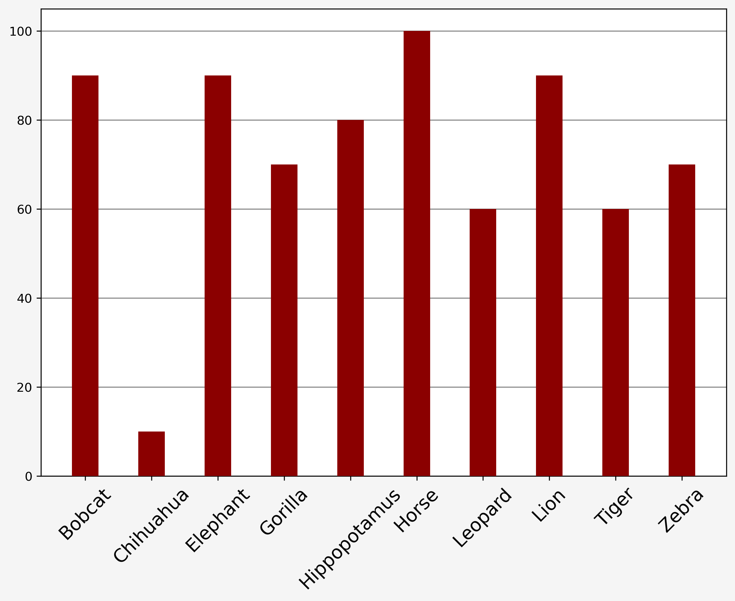
The consistency of the concepts is measured as the percentage of the participants who agreed with the presence of a common pattern across the five visualizations. The overall consistency from the experiments was observed to be 72%. Figure 3 presents the class-wise consistency of the concepts. All classes except chihuahua demonstrate high consistency. Figure 4 presents the visualizations of the concepts and the tags given by the human subjects. It can be observed that the concepts are human interpretable, as the tags are meaningful. The extracted concepts indeed are some of the features of the animals and their natural surroundings according to which humans identify these animals. The tags for the different concepts across the classes labeled by the participants are shown in Table II.


| Class | Interpretable Concept Tags |
|---|---|
| Bobcat | Legs, Ears, Body hair, Back, Ear hair, Grass, Ear tips, Beard |
| Chihuahua | Ears |
| Elephant | Head, Trees, Ground, Eyes, Ears, Face, Trunk, Grass, Water |
| Gorilla | Limbs, Forehead, Grass, Wood, Trees, Head |
| Hippopotamus | Legs, Feet, Water, Back, Background, Sand |
| Horse | Mouth, Nose, Nostrils, Mane, Ears, Grass, Hair, Neck, Back |
| Leopard | Mouth, Grass, Trees, Spots |
| Lion | Lower mane, Trees, Mouth, Back skin, Head, Upper mane, Grass, Paws |
| Tiger | Paws, Ears, Legs, Background, White skin |
| Zebra | Stripes, Grass, Feet, Ground, Ears, Mouth |
IV-C Qualitative Concept Analysis
In Figure 4, it can be seen that various concepts like ears of bobcat in Figure 4(a), face of an elephant in Figure 4(b), etc. being extracted by the PACE framework. A good visual consistency backed up by human subject votes is observed in the extracted concepts. Figure 4(h) tagged as stripes of the zebra seem to consistently highlight the stripes present in the torso region of the animal. A similar observation can be made in Figure 4(g) tagged as spot patterns, the concept highlighted consistently shows the torso of the animal. This qualitatively shows that consistent concept embeddings have been learned as expected.
A few concepts that were marked uninterpretable by the human subjects is presented in Figure 5. Figure 5(a) seems to highlight sand dirt around the legs of the lion and Figure 5(c) highlights grass around the tiger. As it can be seen that the area highlighted to depict the concept itself is very small, only participants with greater attention to details were able to tag such concepts. The majority of the participants deemed it to be uninterpretable. The detection of uninterpretable concepts from the feature maps can be associated to the residuals extracted from the feature map during matrix factorization based explanation techniques [32]. This also proves the effectiveness of PACE that a good approximation of the internals in the feature map has been extracted through interpretable (conceptually analogous to factors in matrix factorization [32]) and uninterpretable concepts (conceptually analogous to residuals in matrix factorization [32]).
Figure 6 shows the concepts extracted by PACE for the VGG19 black-box model trained on the Imagenet-Birds dataset. Salient parts of the birds like feathers of a peacock in Figure 6(e), blue neck in Figure 6(f), eyes of Great Grey Owl in Figure 6(b), its beak in Figure 6(c), toucan’s characteristic colorful bill in Figure 6(h), crest of Sulphur Crested Cockatoo in Figure 6(i), etc. seems to be detected by PACE. These parts are indeed discriminatory features that help distinguish the particular bird species from other bird species. A good visual consistency can also be found in the concepts visualized across different images.


IV-D Explaining Misclassifications
The class-discriminative concepts learned by PACE can be used to explain black-box model misclassifications. Figure 7 presents a few examples of misclassified images and their salient concepts extracted by PACE. Figure 7(a) shows an image of a german shepherd misclassified as a hippopotamus. Understandably, the model uses the concept of water specific to the hippopotamus class for this prediction. Similarly, Figure 7(b) shows a collie being misclassified as a horse due to high support from the concept corresponding to the mane of the horse and Figure 7(c) shows a hippopotamus misclassified as an elephant due to high support from the concept corresponding to the head of the elephant. The explanations show that the model is wrong for the right reasons.


V Conclusion
The PACE framework that learns to extract class-specific concepts relevant to the black-box prediction is proposed.The relevance is formulated such that the explanations are faithful to the black-box prediction by design. The explainer’s applicability on datasets like AWA2 and Imagenet-Birds as well on black-box architectures like VGG16 and VGG19 is experimented. Qualitative and quantitative analyses show that PACE extracts concepts that are consistent and relevant. Extensive human subject experiments show that the proposed framework provides interpretable concepts.
Acknowledgment
The resources provided by ‘PARAM Shivay Facility’ under the National Supercomputing Mission, Government of India at the Indian Institute of Technology, Varanasi, and under Google Tensorflow Research award are gratefully acknowledged.
References
- [1] K. Simonyan and A. Zisserman, “Very deep convolutional networks for large-scale image recognition,” International Conference on Learning Representations (ICLR), vol. 7, 2015.
- [2] K. He, X. Zhang, S. Ren, and J. Sun, “Deep residual learning for image recognition,” in Proceedings of the IEEE Conference on Computer Vision and Pattern Recognition, 2016, pp. 770–778.
- [3] Z. C. Lipton, “The doctor just won’t accept that! interpretable ml symposium,” in 31st conference on Neural Information Processing Systems (NIPS 2017), Long Beach, CA, USA., vol. 1711, 2017.
- [4] 2018 reform of eu data protection rules. European Commission. [Online]. Available: https://ec.europa.eu/commission/sites/beta-political/files/data-protection-factsheet-changes_en.pdf
- [5] R. C. Fong and A. Vedaldi, “Interpretable explanations of black boxes by meaningful perturbation,” in Proceedings of the IEEE International Conference on Computer Vision, 2017, pp. 3429–3437.
- [6] R. Fong, M. Patrick, and A. Vedaldi, “Understanding deep networks via extremal perturbations and smooth masks,” in Proceedings of the IEEE International Conference on Computer Vision, 2019, pp. 2950–2958.
- [7] R. R. Selvaraju, M. Cogswell, A. Das, R. Vedantam, D. Parikh, and D. Batra, “Grad-cam: Visual explanations from deep networks via gradient-based localization,” in Proceedings of the IEEE International Conference on Computer Vision, 2017, pp. 618–626.
- [8] A. Chattopadhyay, A. Sarkar, P. Howlader, and V. N. Balasubramanian, “Grad-cam++: Generalized gradient-based visual explanations for deep convolutional networks,” in 2018 IEEE Winter Conference on Applications of Computer Vision (WACV). IEEE, 2018, pp. 839–847.
- [9] S. Srinivas and F. Fleuret, “Full-gradient representation for neural network visualization,” in Advances in Neural Information Processing Systems, 2019, pp. 4126–4135.
- [10] K. Simonyan, A. Vedaldi, and A. Zisserman, “Deep inside convolutional networks: Visualising image classification models and saliency maps,” in Workshop at International Conference on Learning Representations (ICLR), 2014.
- [11] J. Zhang, S. A. Bargal, Z. Lin, J. Brandt, X. Shen, and S. Sclaroff, “Top-down neural attention by excitation backprop,” International Journal of Computer Vision, vol. 126, no. 10, pp. 1084–1102, 2018.
- [12] H. Wang, Z. Wang, M. Du, F. Yang, Z. Zhang, S. Ding, P. Mardziel, and X. Hu, “Score-cam: Score-weighted visual explanations for convolutional neural networks,” in Proceedings of the IEEE/CVF Conference on Computer Vision and Pattern Recognition Workshops, 2020, pp. 24–25.
- [13] S. Desai and H. G. Ramaswamy, “Ablation-cam: Visual explanations for deep convolutional network via gradient-free localization,” in The IEEE Winter Conference on Applications of Computer Vision, 2020, pp. 983–991.
- [14] J. Adebayo, J. Gilmer, M. Muelly, I. Goodfellow, M. Hardt, and B. Kim, “Sanity checks for saliency maps,” in Advances in Neural Information Processing Systems, 2018, pp. 9505–9515.
- [15] L. Sixt, M. Granz, and T. Landgraf, “When explanations lie: Why modified bp attribution fails,” 37th International Conference on Machine Learning (ICML), 2020.
- [16] C. Chen, O. Li, D. Tao, A. Barnett, C. Rudin, and J. K. Su, “This looks like that: deep learning for interpretable image recognition,” in Advances in Neural Information Processing Systems, 2019, pp. 8928–8939.
- [17] P. Hase, C. Chen, O. Li, and C. Rudin, “Interpretable image recognition with hierarchical prototypes,” in Proceedings of the AAAI Conference on Human Computation and Crowdsourcing, vol. 7, no. 1, 2019, pp. 32–40.
- [18] B. Zhou, A. Khosla, A. Lapedriza, A. Oliva, and A. Torralba, “Learning deep features for discriminative localization,” in Proceedings of the IEEE Conference on Computer Vision and Pattern Recognition, 2016, pp. 2921–2929.
- [19] O. Li, H. Liu, C. Chen, and C. Rudin, “Deep learning for case-based reasoning through prototypes: A neural network that explains its predictions,” in Thirty-Second AAAI Conference on Artificial Intelligence, 2018.
- [20] Y. Wang, H. Su, B. Zhang, and X. Hu, “Learning reliable visual saliency for model explanations,” IEEE Transactions on Multimedia, 2019.
- [21] M. B. Muhammad and M. Yeasin, “Eigen-cam: Visual explanations for deep convolutional neural networks,” SN Computer Science, vol. 2, no. 1, pp. 1–14, 2021.
- [22] M. T. Ribeiro, S. Singh, and C. Guestrin, “Why should i trust you?: Explaining the predictions of any classifier,” in Proceedings of the ACM International Conference on Knowledge Discovery and Data Mining, 2016, pp. 1135–1144.
- [23] S. M. Lundberg and S.-I. Lee, “A unified approach to interpreting model predictions,” in Advances in Neural Information Processing Systems, 2017, pp. 4765–4774.
- [24] M. T. Ribeiro, S. Singh, and C. Guestrin, “Anchors: High-precision model-agnostic explanations,” in Proceedings of the AAAI Conference on Artificial Intelligence, 2018.
- [25] R. Sharma, N. Reddy, V. Kamakshi, N. C. Krishnan, and S. Jain, “Maire–a model-agnostic interpretable rule extraction procedure for explaining classifiers,” arXiv preprint arXiv:2011.01506, 2020.
- [26] H. Lakkaraju, E. Kamar, R. Caruana, and J. Leskovec, “Faithful and customizable explanations of black box models,” in Proceedings of the 2019 AAAI/ACM Conference on AI, Ethics, and Society, 2019, pp. 131–138.
- [27] B. Kim, M. Wattenberg, J. Gilmer, C. Cai, J. Wexler, F. Viegas et al., “Interpretability beyond feature attribution: Quantitative testing with concept activation vectors (tcav),” in International Conference on Machine Learning. PMLR, 2018, pp. 2668–2677.
- [28] A. Ghorbani, J. Wexler, J. Y. Zou, and B. Kim, “Towards automatic concept-based explanations,” in Advances in Neural Information Processing Systems, 2019, pp. 9277–9286.
- [29] W. Wu, Y. Su, X. Chen, S. Zhao, I. King, M. R. Lyu, and Y.-W. Tai, “Towards global explanations of convolutional neural networks with concept attribution,” in Proceedings of the IEEE/CVF Conference on Computer Vision and Pattern Recognition, 2020, pp. 8652–8661.
- [30] A. Nguyen, A. Dosovitskiy, J. Yosinski, T. Brox, and J. Clune, “Synthesizing the preferred inputs for neurons in neural networks via deep generator networks,” in Advances in Neural Information Processing Systems, 2016, pp. 3387–3395.
- [31] C.-K. Yeh, B. Kim, S. Arik, C.-L. Li, T. Pfister, and P. Ravikumar, “On completeness-aware concept-based explanations in deep neural networks,” Advances in Neural Information Processing Systems, vol. 33, 2020.
- [32] R. Zhang, P. Madumal, T. Miller, K. Ehinger, and B. Rubinstein, “Improving interpretability of cnn models using non-negative concept activation vectors,” in Thirty-Fifth AAAI Conference on Artificial Intelligence, 2021.
- [33] F. Schroff, D. Kalenichenko, and J. Philbin, “Facenet: A unified embedding for face recognition and clustering,” in Proceedings of the IEEE Conference on Computer Vision and Pattern Recognition, 2015, pp. 815–823.
- [34] Y. Xian, C. H. Lampert, B. Schiele, and Z. Akata, “Zero-shot learning—a comprehensive evaluation of the good, the bad and the ugly,” IEEE Transactions on Pattern Analysis and Machine Intelligence, vol. 41, no. 9, pp. 2251–2265, 2018.
- [35] O. Russakovsky, J. Deng, H. Su, J. Krause, S. Satheesh, S. Ma, Z. Huang, A. Karpathy, A. Khosla, M. Bernstein et al., “Imagenet large scale visual recognition challenge,” International Journal of Computer Vision, vol. 115, no. 3, pp. 211–252, 2015.
- [36] D. P. Kingma and J. L. Ba, “Adam : A method for stochastic optimization,” International Conference on Learning Representations (ICLR), vol. 7, 2015.