Considering that the invention of the $M_{T2}$ variable started from the attempt of generalizing the transverse mass [13, 14] to deal with two identical decay chains, the algebraic singularity method has emerged from the realization that the phase space of particle momenta is the solution space of the system of kinematic constraints [15]. At collider experiments, we detect only visible particle momenta while missing invisible ones. It can be regarded as the projection of the full phase space of collider event onto the visible subspace. The algebraic singularity method proposes that one can construct singularity variables, which unveil singularities caused by the projection of phase space, by exploiting all the available kinematic constraints in a specific way. Compared to the $M_{T2}$ variable, the algebraic singularity method is a general framework applicable to any decay topology of physics processes containing invisible particles in the final state. The formal description of the algebraic singularity method and the singularity variables are given in Sec. 3.

The author of Ref. [15] mentioned that the algebraic singularity method was initiated due to his desire to understand the $M_{T2}$ variable, and he could eventually derive the $M_{T2}$ variable by using the algebraic singularity method [16]. However, in Ref. [15], the relation between the $M_{T2}$ variable and the algebraic singularity method was not elucidated, and it has never been considered in the following works by different authors [17, 18, 19, 20]. Moreover, in Ref. [21], it has even been argued that $M_{T2}$ is not associated with the singularity variables. On the other hand, in other studies, it has been realized that $M_{T2}$ is not an ad hoc variable, but it sets a boundary of the mass region consistent with the kinematic constraints, which are indeed the defining polynomials of phase space that are used in the algebraic singularity method [22, 23]. These seemingly discrepant arguments and claims have motivated us to examine the relation between the $M_{T2}$ variable and the corresponding singularity variables. If they turn out to be truly orthogonal, the algebraic singularity method will provide new kinematic variables that can be employed in the physics analyses where either or both of the $M_{T2}$ variable and the new variables are applicable. Otherwise, if they are related to each other in any manner, it may still lead to a deeper understanding of the methods. Either way, the algebraic singularity method is an interesting framework for studying various decay topologies with missing energy. We investigate the relation between the $M_{T2}$ and the singularity variable in Sec. 4. Then, the final section is devoted to conclusions.

Before embarking on a discussion of the above issues, a few comments are in order on the applicability of the algebraic singularity method to physics analyses at colliders. As mentioned above, the algebraic singularity method is, in principle, a framework for analyzing the collider events of any decay topology with missing energy rather than a collider variable designed for specific physics processes. The method is still widely unknown and largely unexplored in physics community due to its use of abstract mathematics and the lack of concrete prescriptions with practical examples. A set of worked-out examples of deriving the singularity variables using the method has appeared only very recently [19]. One way to appreciate the potential of the method would be to compare the singularity variables with the known collider variables. In a single two-body decay with an invisible particle in the final state, it has been shown that the well-known transverse mass [13, 14] can be derived by using the method [17, 18, 19, 24]. We will show the derivation of the transverse mass in Sec. 3 by using the Gröbner basis as proposed in the original literature [15] to help the reader understand the method. It has also been found that the $\Delta_{4}$ observable [25, 26], appearing as a factor in four-body phase space [27], corresponds to the singularity variable [19]. We anticipate that our attempt of comparing the $M_{T2}$ with the singularity variables in double-sided decay topology will also help the reader to gain an understanding of the method and to apply the method to find the signals of unexplored decay topologies at colliders.

Though we will not pursue here, there is room for improvement in the way of identifying the singularities of phase space. As noted above, the algebraic singularity method is to capture the kinematic singularities caused by the projection of the full phase space onto the visible subspace. In the original literature, it has been argued that the Gröbner basis of kinematic constraint equations would be particularly useful for identifying singular points on the visible subspace. Meanwhile, the other following works [17, 18, 19, 20] have obtained the singularity variables without employing Gröbner bases. As will be seen in Sec. 3, Gröbner bases have a useful property for identifying singularities. However, the expressions appear to be much more complex than the original system of kinematic constraints, and computing Gröbner bases can be challenging, depending on the form and the numbers of the polynomial equations. We may attempt a different formulation of the method by systematically transforming the system of kinematic constraints into a more refined space of polynomial equations that one can more handily extract singularities. Another possible direction worth exploring is to combine the method with machine learning techniques. The singularity variables can be used as input features for training collider data, and it is conceivable to devise an architecture encoding the algorithm for finding the singularities. We stress that there is much more to explore in further developments and finding the applications of the algebraic singularity method to collider data analyses.

For the double-sided decay topology (2.1) and the hypothesized invisible particle mass $M_{\chi}$, the $M_{T2}$ variable is defined as

	$\displaystyle M_{T2}\equiv$	$\displaystyle\min_{{\bf\it k}_{1T},\,{\bf\it k}_{2T}\in\mathbb{R}^{2}}\Big[\max\Big\{M_{1T}(p_{1T},\,k_{1T},\,M_{\chi}),\,M_{2T}(p_{2T},\,k_{2T},\,M_{\chi})\Big\}\Big]$
		$\displaystyle\text{subject to}\,\,{\bf\it k}_{1T}+{\bf\it k}_{2T}=\not{{\bf\it P}}_{T},$		(2.2)

where $M_{aT}$ are transverse masses given by

$$M_{aT}(p_{aT},\,k_{aT},\,M_{\chi})=\Big[m_{a}^{2}+M_{\chi}^{2}+2\Big(E_{aT}e_{aT}-{\bf\it p}_{aT}\cdot{\bf\it k}_{aT}\Big)\Big]^{1/2}$$

(2.3)

for the final-state particle momenta projected onto the $(1+2)$-dimensional space:

$$p_{aT}=\big(E_{aT},\,{\bf\it p}_{aT}\big),\quad k_{aT}=\big(e_{aT},\,{\bf\it k}_{aT}\big).$$

(2.4)

Here, $E_{aT}=(m_{a}^{2}+\norm{\vb*{p}_{aT}}^{2})^{1/2}$ and $e_{aT}=(M_{\chi}^{2}+\norm{\vb*{k}_{aT}}^{2})^{1/2}$ are transverse energies, and $m_{a}^{2}=p_{a}^{2}$. As will be seen shortly, ${\bf\it k}_{aT}$ in Eq. (2.3) are not the true invisible momenta, nor inputs inserted by hand, but are determined by the minimization of the objective function of $M_{T2}$ under the constraint on the missing transverse momentum,

$$\not{{\bf\it P}}_{T}=-{\bf\it p}_{1T}-{\bf\it p}_{2T}-{\bf\it u}_{T}.$$

(2.5)

Therefore, the $M_{T2}$ variable is a function of visible particle momenta $p_{a}$, missing transverse momentum $\not{{\bf\it P}}_{T}$, and the guessed value of invisible particle mass $M_{\chi}$. What makes the $M_{T2}$ variable useful for mass measurement is that if one inserts a correct value of $M_{\chi}$, its distribution has an endpoint at the parent particle mass, $M_{Y}$:

$$M_{T2}(M_{\chi}=M_{\chi}^{\text{true}})\leq M_{Y}.$$

(2.6)

Because the $M_{T2}$ variable is constructed by only kinematic quantities, it applies to any process, not only the supersymmetric ones, as long as the decay topology given in (2.1) can describe the process of interest.

The calculation of the $M_{T2}$ variable corresponds to the constrained minimization problem of the objective function,

$$f({\bf\it k}_{aT})=\max\Big\{M_{1T}(k_{1T}),\,M_{2T}(k_{2T})\Big\},$$

(2.7)

subject to the equality constraint given by

$${\bf\it c}({\bf\it k}_{a})={\bf\it k}_{1T}+{\bf\it k}_{2T}-\not{{\bf\it P}}_{T}={\bf\it 0}.$$

(2.8)

The problem can be made simpler by eliminating ${\bf\it k}_{2T}$ using the constraint (2.8), ${\bf\it k}_{2T}=\not{{\bf\it P}}_{T}-{\bf\it k}_{1T}$. Then, the objective function becomes

$$f({\bf\it k}_{1T})=\max\Big\{M_{1T}(e_{1T},\,{\bf\it k}_{1T}),\,M_{2T}(e_{2T},\,\not{{\bf\it P}}_{T}-{\bf\it k}_{1T})\Big\},$$

(2.9)

where $e_{2T}=(M_{\chi}^{2}+\norm{\slashed{\vb*{P}}_T - \vb*{k}_{1T}}^{2})^{1/2}$. The calculation of $M_{T2}$ has now become an unconstrained minimization on a function of two variables, ${\bf\it k}_{1T}=(k_{1x}$, $k_{1y})$. The value of ${\bf\it k}_{1T}$ at the minimum of the objective function $f({\bf\it k}_{1T})$ is the $M_{T2}$ solution to the invisible particle momenta,

$$\widetilde{{\bf\it k}}_{1T}=\argmin_{{\bf\it k}_{1T}\in\mathbb{R}^{2}}f({\bf\it k}_{1T}).$$

(2.10)

Here, $\argmin$ stands for the argument of minimum, i.e., the point ${\bf\it k}_{1T}$ for which $f({\bf\it k}_{1T})$ attains its minimum. It has been found that $\widetilde{{\bf\it k}}_{1T}$ can provide a good approximation to the invisible particle momenta along with on-shell mass constraints [10]. Even though we have converted to a simpler problem of unconstrained minimization over the fewer degrees of freedom, one should employ a numerical algorithm, such as the quasi-Newton method, to obtain the value of $M_{T2}$. We refer the reader to Refs. [28, 29] for a review of the $M_{T2}$ variable in terms of minimization problems and the numerical algorithms feasible for solving the problem.

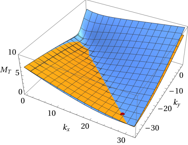
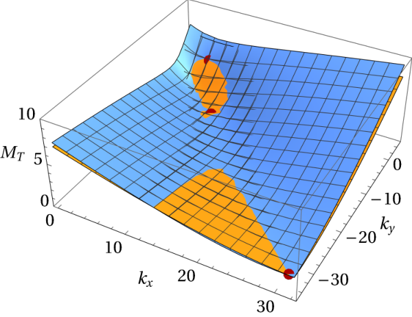
Although we use numerical algorithms in practical physics analyses, it is worth inspecting the analytic property of the $M_{T2}$ variable. Because the objective function of $M_{T2}$ is a convex function over the invisible particle momenta ${\bf\it k}_{aT}$ [29, 30], it has a unique local minimum, which is automatically a global minimum. Furthermore, as the transverse masses in Eq. (2.3) are also convex functions, the $M_{T2}$ value is determined by the configuration of the two convex functions, as depicted in Fig. 1.

The stationary points of the transverse masses can be obtained by requiring their gradients,

	$\displaystyle\frac{\partial M_{1T}^{2}}{\partial{\bf\it k}_{1T}}$	$\displaystyle=2\left[\frac{E_{1T}}{e_{1T}}{\bf\it k}_{1T}-{\bf\it p}_{1T}\right],$
	$\displaystyle\frac{\partial M_{2T}^{2}}{\partial{\bf\it k}_{1T}}$	$\displaystyle=2\left[-\frac{E_{2T}}{e_{2T}}\left(\not{{\bf\it P}}_{T}-{\bf\it k}_{1T}\right)+{\bf\it p}_{2T}\right],$		(2.11)

to be vanishing. Here, we have eliminated ${\bf\it k}_{2T}$ by using the constraint on missing transverse momentum given in Eq. (2.8). At each stationary point, we have the global minimum of corresponding transverse mass as follows:

	$\displaystyle M_{1T}$	$\displaystyle=m_{1}+M_{\chi}\quad\text{when }{\bf\it k}_{1T}=\frac{e_{1T}}{E_{1T}}{\bf\it p}_{1T},$
	$\displaystyle M_{2T}$	$\displaystyle=m_{2}+M_{\chi}\quad\text{when }{\bf\it k}_{1T}=\not{{\bf\it P}}_{T}-\frac{e_{2T}}{E_{2T}}{\bf\it p}_{2T}.$		(2.12)

The configuration of the transverse masses are determined by the visible particle momenta and missing transverse momentum. In the configuration depicted in the left panel of Fig. 1, the $M_{T2}$ value is given by

$$M_{T2}=M_{1T}=M_{2T}$$

(2.13)

if both conditions below are satisfied:

	$\displaystyle M_{2T}$	$\displaystyle\geq m_{1}+M_{\chi}\quad\text{when }{\bf\it k}_{1T}=\frac{e_{1T}}{E_{1T}}{\bf\it p}_{1T},$
	$\displaystyle M_{1T}$	$\displaystyle\geq m_{2}+M_{\chi}\quad\text{when }{\bf\it k}_{1T}=\not{{\bf\it P}}_{T}-\frac{e_{2T}}{E_{2T}}{\bf\it p}_{2T}.$		(2.14)

This is called the balanced configuration. Otherwise, if any of the conditions is violated, the $M_{T2}$ value is given by the larger of the two global minima of the transverse masses,

$$M_{T2}=\max\Big[m_{1}+M_{\chi},\,m_{2}+M_{\chi}\Big].$$

(2.15)

See the right panel of Fig. 1. In this case, Eq. (2.13) does not hold, and it is termed the unbalanced configuration. The balanced and the unbalanced configurations span all possible cases of the $M_{T2}$ solution: an event can be in either a balanced or an unbalanced configuration.

The general analytic expression of $M_{T2}$ in balanced configurations is hitherto unknown except for some special cases [31, 32, 33, 34, 35], whereas the expression of the $M_{T2}$ variable in the case of the unbalanced configuration is given by Eq. (2.15).¹¹ 1 On the other hand, the analytic expressions for the endpoint of the $M_{T2}$ distribution are known [36, 37, 32, 38, 39, 40]. When the upstream momentum in the decay topology (2.1) is vanishing, the expression of $M_{T2}$ in balanced configurations has been identified, and it is given as follows [31, 32]:

$$M_{T2}^{2}=M_{\chi}^{2}+A_{T}+\sqrt{\left(1+\frac{4M_{\chi}^{2}}{2A_{T}-m_{1}^{2}-m_{2}^{2}}\right)\left(A_{T}^{2}-m_{1}^{2}m_{2}^{2}\right)},$$

(2.16)

where

$$A_{T}=E_{1T}E_{2T}+{\bf\it p}_{1T}\cdot{\bf\it p}_{2T}.$$

(2.17)

Likewise, the analytic expression of the $M_{T2}$ solution, $\widetilde{{\bf\it k}}_{1T}$, applicable in all respects, remains to be identified. In the case of vanishing upstream momentum, the derivation of the $M_{T2}$ solution is capable but quite involved [41]. Nonetheless, in the plain case where the visible particles are massless, $m_{1}=m_{2}=0$, we can use a simple ansatz for the form of the $M_{T2}$ solution in the balanced configuration, given as follows:

$$\widetilde{{\bf\it k}}_{1T}=\frac{1}{2}\Big[\left(\alpha_{T}-1\right){\bf\it p}_{1T}-\left(\alpha_{T}+1\right){\bf\it p}_{2T}\Big],$$

(2.18)

where $\alpha_{T}$ is a function of the visible particle momenta and the invisible particle mass $M_{\chi}$. By substituting the above expression into

$$M_{T2}^{2}=\frac{M_{1T}^{2}+M_{2T}^{2}}{2}$$

(2.19)

and using the expression of $M_{T2}$ in Eq. (2.16) with $m_{1}=m_{2}=0$, we get

$$\alpha_{T}=\sqrt{1+\frac{2M_{\chi}^{2}}{A_{T}}}.$$

(2.20)

Here, $A_{T}=\norm{\vb*{p}_{1T}}\norm{\vb*{p}_{2T}}+{\bf\it p}_{1T}\cdot{\bf\it p}_{2T}$. If the invisible particle is massless as well, $M_{\chi}=0$, the expression (2.18) further simplifies as

$$\widetilde{{\bf\it k}}_{1T}=-{\bf\it p}_{2T}.$$

(2.21)

Because we here assume that the upstream momentum is vanishing, the missing transverse momentum is given by the negative vector sum of the visible particle momenta from the decays of $Y$ and $\bar{Y}$, $\not{{\bf\it P}}_{T}=-{\bf\it p}_{1T}-{\bf\it p}_{2T}$. Therefore, the invisible transverse momentum of the second decay chain is given by

$$\widetilde{{\bf\it k}}_{2T}=-{\bf\it p}_{1T}.$$

(2.22)

This expression matches that identified in the study of $M_{T2}$ for the $h\to WW\to\ell^{+}\nu\ell^{-}\bar{\nu}$ process, where the visible and invisible particles in the final state are all massless [42, 43]. We will revisit the fully massless case in the last section before conclusions.

In missing energy events, not only in the double-sided decay topology, the phase space can be decomposed into $\{(k_{a}$, $p_{b})\}$. By measuring the visible particle momenta $p_{b}$ while missing the invisible particle momenta $k_{a}$, the phase space is projected onto the visible subspace $\{p_{b}\}$. The projection leads to singularities in the visible subspace, where the full phase space $\{(k_{a}$, $p_{b})\}$ is folded. The event number density changes abruptly at the singularities, and they can appear in several different forms such as wall or cusp.

The salient point of the algebraic singularity method is that the singularities can be identified by constructing the Jacobian matrix of the constraint polynomials $g_{i}$,

$$J_{ij}=\frac{\partial g_{i}}{\partial k_{j}}.$$

(3.2)

Here, the index $j$ runs over the energy-momentum components of the invisible particles, $k_{a}=(e_{a}$, $k_{ax}$, $k_{ay}$, $k_{az})$. The algebraic singularity method is based on the observation that the Jacobian matrix (3.2) has reduced rank at singularities. In other words, one or more row vectors of the Jacobian matrix are linearly dependent at singularities. Note that the Jacobian matrix defines a linear mapping, which best approximates $g_{i}$ at the point $k_{a}$. If the Jacobian matrix has reduced rank, its image of the linear mapping is smaller, and the approximation by the mapping is no more valid. Consequently, having reduced rank indicates a singular behavior of $g_{i}$ near the point $k_{a}$. In the subsequent works by different authors [17, 18, 19, 20], the reduced rank condition has been referred to as “singularity condition.” The Jacobian matrix is a square matrix if the number of polynomials in Eq. (3.1) equals to that of unknowns. In this case, the reduced rank condition is equivalent to the vanishing determinant of the Jacobian matrix, as studied in Refs. [19, 20].

In general, the defining polynomials of phase space form a system of nonlinear coupled equations, and consequently, finding the reduced rank condition of the Jacobian matrix is a nontrivial task. Affine varieties are defined by ideals, which are the sets of all polynomials having the same solution space. The ideal generated by a finite set of polynomials is analogous to the span of a finite number of vectors in linear algebra. Indeed, the finite set of polynomials is termed a basis of the ideal. A given ideal may have many different bases. In Ref. [15], it is emphasized that Gröbner bases, also known as the standard bases, can be particularly useful for examining the reduced rank condition of the Jacobian matrix because it can make the matrix a row echelon form. It is analogous to Gaussian elimination for linear systems. Then, to identify the singularities, we set some of the diagonal components of the Jacobian matrix in the Gröbner basis to be vanishing and check whether the row vectors of the Jacobian matrix with vanishing diagonal component are linearly dependent. Unfortunately, the analytic calculation of Gröbner bases can be challenging if the number of polynomials is large, and thus one typically employs dedicated algorithms such as Buchberger’s algorithm [44]. In the case of the double-sided decay topology in (2.1), we can manage to obtain the corresponding Gröbner basis analytically, as done in Ref. [15]. We will see the expressions of the Gröbner basis in the following subsection.

Having identified the singularities by imposing the reduced rank condition, we can construct an optimized kinematic variable, named singularity coordinate. It is required to be zero at singularities and is perpendicular to the singularity hypersurface in the visible phase space. Collider events near the singularities are projected onto the coordinate. It is also normalized so that the events with the same distance to the singularities give the same value. It is called a coordinate as it determines the positions of collider events on the singularity hypersurface. Singularity coordinate is an implicit variable because it depends on the masses of the unknown particles such as $Y$ and $\chi$ in the decay topology (2.1). If trial mass values have correctly been chosen, the singularity coordinate maximizes singular features. Consequently, we can deduce the mass spectrum of unknown particles by comparing several competing hypotheses using the singularity coordinate.

Although the formal definition of singularity coordinates is given in Ref. [15], it lacks a practical recipe for constructing them. It has later been supplemented by the studies of applying the algebraic singularity method to several physics processes of various decay topologies: single $W$ production $W\to\ell\nu$ [17], the dileptonic Higgs channel $h\to WW\to\ell^{+}\nu\ell^{-}\bar{\nu}$ [18], heavy Higgs boson decaying to a top-quark pair $H/A\to t\bar{t}\to bW\bar{b}W\to b\ell^{+}\nu\,\bar{b}\ell^{-}\bar{\nu}$ [20], and various single- and double-sided decay topologies [19]. In the studies, singularity coordinates are called interchangeably with singularity variables. The latter are also functions of visible particle momenta and unknown particle masses, but it has mass dimension one. The singularity variables enable us directly to measure the unknown particle masses by identifying the peak or the endpoints of their distributions. By contrast, the singularity coordinates can have mass dimensions much higher than one, and one can estimate the unknown particle masses by performing template fitting of the distribution shapes. We can hardly extract the mass information directly from the distribution. Therefore, singularity variables are more straightforward and intuitive to use in physics analyses than singularity coordinates. In this article, we distinguish the singularity coordinates and the singularity variables and concentrate on the latter.

Before examining the singularity variable for the double-sided decay topology in (2.1), we take a look into the singularity variable for the simpler decay topology in order to help facilitate the understanding of the algebraic singularity method. Consider a single-sided two-body decay topology, where one of the decay products is invisible,

$$Y\longrightarrow v(p)\chi(k).$$

(3.3)

The kinematic constraints of the decay topology are given as follows:

	$\displaystyle k^{2}$	$\displaystyle=M_{\chi}^{2},$
	$\displaystyle{(p+k)}^{2}$	$\displaystyle=M_{Y}^{2},$
	$\displaystyle{\bf\it k}_{T}$	$\displaystyle=\not{{\bf\it P}}_{T},$		(3.4)

where $k=(e$, ${\bf\it k}_{T}$, $k_{z})=(e$, $k_{x}$, $k_{y}$, $k_{z})$ contains the unknowns of the system, and $p=(E$, ${\bf\it p}_{T}$, $p_{z})=(E$, $p_{x}$, $p_{y}$, $p_{z})$ is the visible particle momentum of the given collider event. Using the lexicographic ordering $k_{x}\succ k_{y}\succ k_{z}\succ e$, we find that the Gröbner basis of the system is given by

	$\displaystyle g_{1}=$	$\displaystyle~k_{x}-\not{P}_{x},$
	$\displaystyle g_{2}=$	$\displaystyle~k_{y}-\not{P}_{y},$
	$\displaystyle g_{3}=$	$\displaystyle-2p_{z}k_{z}+2Ee-\left(M_{Y}^{2}-M_{\chi}^{2}-m^{2}+2{\bf\it p}_{T}\cdot\not{{\bf\it P}}_{T}\right),$
	$\displaystyle g_{4}=$	$\displaystyle-4(E^{2}-p_{z}^{2})e^{2}+4E\left(M_{Y}^{2}-M_{\chi}^{2}-m^{2}+2{\bf\it p}_{T}\cdot\not{{\bf\it P}}_{T}\right)e$
		$\displaystyle-(M_{Y}^{2}-M_{\chi}^{2}-m^{2}+2{\bf\it p}_{T}\cdot\not{{\bf\it P}}_{T})^{2}-4p_{z}^{2}(M_{\chi}^{2}+\norm{\slashed{\vb*{P}}_T}^{2}),$		(3.5)

where $m^{2}=p^{2}$. We have four constraint equations and four unknowns. Therefore, the Jacobian is a $4\times 4$ matrix given as follows:

$$J_{ij}=\frac{\partial g_{i}}{\partial k_{j}}=\begin{pmatrix}1&&&\\ &1&&\\ &&-2p_{z}&2E\\ &&&-8(E^{2}-p_{z}^{2})e+4E\left(M_{Y}^{2}-M_{\chi}^{2}-m^{2}+2{\bf\it p}_{T}\cdot\not{{\bf\it P}}_{T}\right)\end{pmatrix}.$$

(3.6)

As mentioned earlier, taking the Gröbner basis renders the Jacobian matrix having the row echelon form. Except for the soft singularity where $p_{z}=0$, the reduced rank condition requires the fourth diagonal term of $J$ to be vanishing,

$$0=J_{44}=8p_{z}Ee\left(\frac{p_{z}}{E}-\frac{k_{z}}{e}\right).$$

(3.7)

Here, we have used the constraints in (3.4) to eliminate $M_{Y}^{2}$ and $\not{{\bf\it P}}_{T}$. Note that Eq. (3.7) is equivalent to the relation that

$$\frac{p_{z}}{E_{T}}=\frac{k_{z}}{e_{T}}$$

(3.8)

if $p_{z}$, $E$, and $e$ are all nonzero. By using the relation, we get

$\displaystyle M_{Y}^{2}=m^{2}+M_{\chi}^{2}+2\left(E_{T}e_{T}-{\bf\it p}_{T}\cdot{\bf\it k}_{T}\right),$

(3.9)

where ${\bf\it k}_{T}=\not{{\bf\it P}}_{T}$. The expression on the right-hand side is nothing but the transverse mass squared for the $v$ and $\chi$ system. It shows that the transverse mass corresponds to the singularity variable of the decay topology (3.3), as shown in Refs. [24, 17, 18, 19]. The transverse mass is the invariant mass in the $(1+2)$-dimensional space, and the algebraic singularity method tells us that it is an optimized variable. The Jacobian peak in the transverse mass distribution is indeed a feature of singularity.

Because both $M_{T2}$ and singularity variables do not have analytic expressions in general cases, the comparison of the two different types of variables is not a straightforward task. If either or both of $\partial M_{1T}/\partial{\bf\it k}_{1T}$ and $\partial M_{2T}/\partial{\bf\it k}_{1T}$ are vanishing, the condition (3.24) is trivially satisfied, but it does not always lead to the balanced configuration, $M_{1T}=M_{2T}$. In the case where visible particle systems are massless and upstream momentum is vanishing, we have seen that the $M_{T2}$ solution to the invisible particle momenta in balanced configurations is given by Eq. (2.18). Indeed, when $m_{1}=m_{2}=0$, the condition (2.14) always holds, and thus every collider event is in a balanced configuration. One can see that the analytic expression of the $M_{T2}$ solution (2.18) satisfies both conditions, Eqs. (3.22) and (3.24). Therefore, in this particular case, we have proven that the singularity variables contain the $M_{T2}$ variable.

References

- [1] C. G. Lester and D. J. Summers, “Measuring masses of semiinvisibly decaying particles pair produced at hadron colliders,” Phys. Lett. B 463 (1999) 99–103, arXiv:hep-ph/9906349.
- [2] A. Barr, C. Lester, and P. Stephens, “: The Truth behind the glamour,” J. Phys. G 29 (2003) 2343–2363, arXiv:hep-ph/0304226.
- [3] W. S. Cho, K. Choi, Y. G. Kim, and C. B. Park, “Measuring the top quark mass with at the LHC,” Phys. Rev. D 78 (2008) 034019, arXiv:0804.2185 [hep-ph].
- [4] CDF Collaboration, T. Aaltonen et al., “Measurement of the Top Quark Mass in the Dilepton Channel Using at CDF,” Phys. Rev. D 81 (2010) 031102, arXiv:0911.2956 [hep-ex].
- [5] D. Guadagnoli and C. B. Park, “-reconstructed invisible momenta as spin analizers, and an application to top polarization,” JHEP 01 (2014) 030, arXiv:1308.2226 [hep-ph].
- [6] CMS Collaboration, A. M. Sirunyan et al., “Measurement of the top quark mass in the dileptonic decay channel using the mass observables , , and in pp collisions at TeV,” Phys. Rev. D 96 no. 3, (2017) 032002, arXiv:1704.06142 [hep-ex].
- [7] A. J. Barr and C. Gwenlan, “The Race for supersymmetry: Using for discovery,” Phys. Rev. D 80 (2009) 074007, arXiv:0907.2713 [hep-ph].
- [8] ATLAS Collaboration, G. Aad et al., “Search for new phenomena in events with two opposite-charge leptons, jets and missing transverse momentum in pp collisions at = 13 TeV with the ATLAS detector,” JHEP 04 (2021) 165, arXiv:2102.01444 [hep-ex].
- [9] CMS Collaboration, A. Tumasyan et al., “Search for electroweak production of charginos and neutralinos in proton-proton collisions at 13 TeV,” arXiv:2106.14246 [hep-ex].
- [10] W. S. Cho, K. Choi, Y. G. Kim, and C. B. Park, “-assisted on-shell reconstruction of missing momenta and its application to spin measurement at the LHC,” Phys. Rev. D 79 (2009) 031701, arXiv:0810.4853 [hep-ph].
- [11] W. S. Cho, J. E. Kim, and J.-H. Kim, “Amplification of endpoint structure for new particle mass measurement at the LHC,” Phys. Rev. D 81 (2010) 095010, arXiv:0912.2354 [hep-ph].
- [12] W. S. Cho, J. S. Gainer, D. Kim, K. T. Matchev, F. Moortgat, L. Pape, and M. Park, “On-shell constrained variables with applications to mass measurements and topology disambiguation,” JHEP 08 (2014) 070, arXiv:1401.1449 [hep-ph].
- [13] V. D. Barger, A. D. Martin, and R. J. N. Phillips, “Perpendicular Mass From Decay,” Z. Phys. C 21 (1983) 99.
- [14] J. Smith, W. L. van Neerven, and J. A. M. Vermaseren, “The Transverse Mass and Width of the Boson,” Phys. Rev. Lett. 50 (1983) 1738.
- [15] I.-W. Kim, “Algebraic Singularity Method for Mass Measurement with Missing Energy,” Phys. Rev. Lett. 104 (2010) 081601, arXiv:0910.1149 [hep-ph].
- [16] I.-W. Kim and C. B. Park. Private communication.
- [17] A. Rujula and A. Galindo, “Measuring the W-Boson mass at a hadron collider: a study of phase-space singularity methods,” JHEP 08 (2011) 023, arXiv:1106.0396 [hep-ph].
- [18] A. De Rujula and A. Galindo, “Singular ways to search for the Higgs boson,” JHEP 06 (2012) 091, arXiv:1202.2552 [hep-ph].
- [19] K. T. Matchev and P. Shyamsundar, “Singularity Variables for Missing Energy Event Kinematics,” JHEP 04 (2020) 027, arXiv:1911.01913 [hep-ph].
- [20] C. B. Park, “A singular way to search for heavy resonances in missing energy events,” JHEP 07 (2020) 089, arXiv:2005.12297 [hep-ph].
- [21] D. Kim, K. Kong, K. T. Matchev, M. Park, and P. Shyamsundar, “Deep-Learned Event Variables for Collider Phenomenology,” arXiv:2105.10126 [hep-ph].
- [22] H.-C. Cheng and Z. Han, “Minimal Kinematic Constraints and ,” JHEP 12 (2008) 063, arXiv:0810.5178 [hep-ph].
- [23] A. J. Barr, B. Gripaios, and C. G. Lester, “Transverse masses and kinematic constraints: from the boundary to the crease,” JHEP 11 (2009) 096, arXiv:0908.3779 [hep-ph].
- [24] New Physics Working Group Collaboration, G. Brooijmans et al., “New Physics at the LHC. A Les Houches Report: Physics at TeV Colliders 2009 - New Physics Working Group,” in 6th Les Houches Workshop on Physics at TeV Colliders, pp. 191–380. 5, 2010. arXiv:1005.1229 [hep-ph].
- [25] P. Agrawal, C. Kilic, C. White, and J.-H. Yu, “Improved Mass Measurement Using the Boundary of Many-Body Phase Space,” Phys. Rev. D 89 no. 1, (2014) 015021, arXiv:1308.6560 [hep-ph].
- [26] D. Debnath, J. S. Gainer, C. Kilic, D. Kim, K. T. Matchev, and Y.-P. Yang, “Enhancing the discovery prospects for SUSY-like decays with a forgotten kinematic variable,” JHEP 05 (2019) 008, arXiv:1809.04517 [hep-ph].
- [27] N. Byers and C. N. Yang, “Physical Regions in Invariant Variables for n Particles and the Phase-Space Volume Element,” Rev. Mod. Phys. 36 no. 2, (1964) 595–609.
- [28] W. S. Cho, J. S. Gainer, D. Kim, S. H. Lim, K. T. Matchev, F. Moortgat, L. Pape, and M. Park, “OPTIMASS: A Package for the Minimization of Kinematic Mass Functions with Constraints,” JHEP 01 (2016) 026, arXiv:1508.00589 [hep-ph].
- [29] C. B. Park, “YAM2: Yet another library for the variables using sequential quadratic programming,” Comput. Phys. Commun. 264 (2021) 107967, arXiv:2007.15537 [hep-ph].
- [30] S. H. Lim, “Identifying the production process of new physics at colliders; symmetric or asymmetric?,” JHEP 06 (2016) 105, arXiv:1603.01981 [hep-ph].
- [31] C. Lester and A. Barr, “: Mass scale measurements in pair-production at colliders,” JHEP 12 (2007) 102, arXiv:0708.1028 [hep-ph].
- [32] W. S. Cho, K. Choi, Y. G. Kim, and C. B. Park, “Measuring superparticle masses at hadron collider using the transverse mass kink,” JHEP 02 (2008) 035, arXiv:0711.4526 [hep-ph].
- [33] W. S. Cho, K. Choi, Y. G. Kim, and C. B. Park, “Mass and Spin Measurement with and MAOS Momentum,” Nucl. Phys. B Proc. Suppl. 200-202 (2010) 103–112, arXiv:0909.4853 [hep-ph].
- [34] C. G. Lester, “The stransverse mass, , in special cases,” JHEP 05 (2011) 076, arXiv:1103.5682 [hep-ph].
- [35] C. H. Lally and C. G. Lester, “Properties of in the massless limit,” arXiv:1211.1542 [hep-ph].
- [36] W. S. Cho, K. Choi, Y. G. Kim, and C. B. Park, “Gluino Stransverse Mass,” Phys. Rev. Lett. 100 (2008) 171801, arXiv:0709.0288 [hep-ph].
- [37] A. J. Barr, B. Gripaios, and C. G. Lester, “Weighing Wimps with Kinks at Colliders: Invisible Particle Mass Measurements from Endpoints,” JHEP 02 (2008) 014, arXiv:0711.4008 [hep-ph].
- [38] M. Burns, K. Kong, K. T. Matchev, and M. Park, “Using Subsystem for Complete Mass Determinations in Decay Chains with Missing Energy at Hadron Colliders,” JHEP 03 (2009) 143, arXiv:0810.5576 [hep-ph].
- [39] P. Konar, K. Kong, K. T. Matchev, and M. Park, “Dark Matter Particle Spectroscopy at the LHC: Generalizing to Asymmetric Event Topologies,” JHEP 04 (2010) 086, arXiv:0911.4126 [hep-ph].
- [40] R. Mahbubani, K. T. Matchev, and M. Park, “Re-interpreting the Oxbridge stransverse mass variable in general cases,” JHEP 03 (2013) 134, arXiv:1212.1720 [hep-ph].
- [41] W. S. Cho, K. Choi, and C. B. Park, “The solution to the invisible particle momenta in balanced configuration,” Unpublished.
- [42] K. Choi, S. Choi, J. S. Lee, and C. B. Park, “Reconstructing the Higgs boson in dileptonic W decays at hadron collider,” Phys. Rev. D 80 (2009) 073010, arXiv:0908.0079 [hep-ph].
- [43] K. Choi, J. S. Lee, and C. B. Park, “Measuring the Higgs boson mass with transverse mass variables,” Phys. Rev. D 82 (2010) 113017, arXiv:1008.2690 [hep-ph].
- [44] B. Buchberger, “A theoretical basis for the reduction of polynomials to canonical forms,” ACM SIGSAM Bulletin 10 (1976) 19–29.
- [45] CMS Collaboration, G. L. Bayatian et al., “CMS technical design report, volume II: Physics performance,” J. Phys. G 34 no. 6, (2007) 995–1579.
- [46] M. M. Nojiri, Y. Shimizu, S. Okada, and K. Kawagoe, “Inclusive transverse mass analysis for squark and gluino mass determination,” JHEP 06 (2008) 035, arXiv:0802.2412 [hep-ph].
- [47] A. Rajaraman and F. Yu, “A New Method for Resolving Combinatorial Ambiguities at Hadron Colliders,” Phys. Lett. B 700 (2011) 126–132, arXiv:1009.2751 [hep-ph].
- [48] P. Baringer, K. Kong, M. McCaskey, and D. Noonan, “Revisiting Combinatorial Ambiguities at Hadron Colliders with ,” JHEP 10 (2011) 101, arXiv:1109.1563 [hep-ph].
- [49] K. Choi, D. Guadagnoli, and C. B. Park, “Reducing combinatorial uncertainties: A new technique based on variables,” JHEP 11 (2011) 117, arXiv:1109.2201 [hep-ph].
- [50] D. Debnath, D. Kim, J. H. Kim, K. Kong, and K. T. Matchev, “Resolving Combinatorial Ambiguities in Dilepton Event Topologies with Constrained Variables,” Phys. Rev. D 96 no. 7, (2017) 076005, arXiv:1706.04995 [hep-ph].
- [51] C. B. Park, “Reconstructing the heavy resonance at hadron colliders,” Phys. Rev. D 84 (2011) 096001, arXiv:1106.6087 [hep-ph].
- [52] C. G. Lester and B. Nachman, “Bisection-based asymmetric MT2 computation: a higher precision calculator than existing symmetric methods,” JHEP 03 (2015) 100, arXiv:1411.4312 [hep-ph].
- [53] ATLAS Collaboration, G. Aad et al., “Search for electroweak production of charginos and sleptons decaying into final states with two leptons and missing transverse momentum in TeV collisions using the ATLAS detector,” Eur. Phys. J. C 80 no. 2, (2020) 123, arXiv:1908.08215 [hep-ex].
- [54] CMS Collaboration, A. M. Sirunyan et al., “Search for supersymmetry in final states with two oppositely charged same-flavor leptons and missing transverse momentum in proton-proton collisions at 13 TeV,” JHEP 04 (2021) 123, arXiv:2012.08600 [hep-ex].
- [55] T. Sjöstrand, S. Ask, J. R. Christiansen, R. Corke, N. Desai, P. Ilten, S. Mrenna, S. Prestel, C. O. Rasmussen, and P. Z. Skands, “An introduction to PYTHIA 8.2,” Comput. Phys. Commun. 191 (2015) 159–177, arXiv:1410.3012 [hep-ph].