When Jones [6] introduced the Jones polynomial, he [6, page 360, §10] tried to define a 3-manifold invariant associated with the Jones polynomial, and succeeded in some cases. After that, Witten [24] wrote a path integral for a 3-manifold invariant. Reshetikhin and Turaev [21] defined a 3-manifold invariant via surgery and quantum groups that one can view as a mathematically rigorous definition of the path integral. Kirby and Melvin and Lickorish and Kauffman and Lins [14, 17, 18, 11] continue this work. Such 3-manifold invariants are called quantum invariants.

The above quantum invariants were defined for closed oriented 3-manifolds. In this paper we introduce topological quantum invariants, surface link quantum invariants, of compact oriented 3-manifolds with boundary where the boundary is a disjoint union of two identical surfaces. In this paper 3-manifolds with boundary mean connected compact oriented 3-manifolds with non-vacuous boundary and surfaces mean connected closed oriented surfaces. See §9. We explain how to use Kirby calculus for such manifolds, and we use the diagrammatics of virtual knots and links to define these invariants.

The surface link quantum invariants defined here are new, nontrivial, and calculable examples of quantum invariants of 3-manifolds with non-vacuous boundary.

Our new invariants, surface link quantum invariants, give new invariants of classical links in the 3-sphere in the following sense: Consider a link $L$ in $S^{3}$ of two components. The complement of a tubular neighborhood of $L$ is a manifold whose boundary consists in two copies of a torus. Our invariants apply to this case of bounded manifold and give new invariants of the given link of two components. We apply it and also obtain invariants of 1-component links. See §10. In this way, the theory of virtual links is used to construct new invariants of classical links in the 3-sphere.

It should be mentioned that the application of virtual knots to the calculation of these invariants is non-trivial and necessary. The Dye-Kauffman [3] handling for Kirby calculus and Temperley-Lieb Recoupling Theory for virtual link diagrams allows us to give specific formulas for our invariants for manifolds obtained by surgery on framed links embedded in a thickened surface. Just as the Jones polynomial can be calculated for links in thickened surfaces via virtual knot combinatorics, so can these surgery invariants be so calculated. Note that in order to apply the virtual diagrammatic Kirby calculus, we need to make our definitions so that the Roberts circumcision move $\mathcal{O}_{3}$ is not needed. This we do by choosing a special surgical normalization as described below. One result of the normalization is that one cannot take any framed virtual diagram for our purposes, but any diagram can be modified so that the normalization is in effect. In this paper we provide the definitions and frameworks. In the sequel to this paper, specific calculations and applications will be provided.

In the sections to follow we address a number of issues. We show how to specify framings for the links in a thickened surface so that one can apply surgery. We explain the results of Justin Roberts [23] for surgery on three manifolds that are relevant and that apply for our use of Kirby Calculus. It should be noted that Robert’s results use an extra move for his version of Kirby Calculus here denoted as $\mathcal{O}_{3}.$ We show that the three manifolds that we construct can be chosen to have associated four manifolds that are simply connected, and that in this category, the topological types of these three manifolds are classified by just the first two of the moves $\mathcal{O}_{1}$ and $\mathcal{O}_{2}.$ Restricting ourselves to this category of three-manifolds, the first two moves correspond to the classical Kirby Calculus and to the generalized Kirby Calculus for virtual diagrams.

Note that we work only with closed oriented 3-manifolds that bound specific simply connected compact 4-manifolds, usually with these 4-manifolds corresponding to surgery instructions on a given link. Thus we concentrate on framed links that represent given 3-manifolds with boundary and that represent simply connected 4-manifolds.

In this way, we are able to apply Robert’s results and make the connection between the topological types in a category of three manifolds and the Kirby Calculus classes of virtual link diagrams. With these connections in place, the paper ends with a description of the construction of Witten-Reshetikhin-Turaev invariants that apply, via virtual Kirby Calculus, to our category of three-manifolds.

In this paper, we give the theory of these new invariants and the proofs of their validity. Explicit calculations of examples will be done in a sequel to the present paper.

We shall define new topological quantum invariants, surface link quantum invariant, of 3-manifolds $M$ with the boundary condition $\mathcal{B}$. More precisely, our invariants are defined for elements of the following set $\mathcal{Z}$ $($respectively, $\mathcal{Y}$$).$

$\mathcal{Z}=\{\text{Connected compact oriented 3-manifolds with boundary}$

$\text{with the boundary condition $\mathcal{B}$}\}/\sim$,

$\mathcal{Y}=\{\text{Connected compact oriented 3-manifolds with boundary}$

$\text{with the boundary condition $\mathcal{B}$}\}/\sim$,

Note that there is a natural map from $\mathcal{Z}$ to $\mathcal{Y}$.

We need the condition $\mathcal{B}$ in Theorem 5.4 when we apply Theorem 4.1. See also Remark 4.2.

See Figure 3.1 for an example. We draw a framed link in the surface which is the projection of a thickened surface. The place where a circle is cut means which segments there goes over or down, as usual.

We can define linking number for two components of any 2-component link in any thickened surface. See Remark 3.3.

A framed link $L^{fr}$ in $F\times[-1,1]$ together with the symplectic basis condition $\mathcal{F}$ then represents a connected compact oriented 3-manifold with the boundary $F\amalg-F$ with the boundary condition $\mathcal{B}$ naturally.

This framed link also represents a 4-manifold with boundary.

We need the conditions $\mathcal{B}$ and $\mathcal{F}$ in Theorem 5.4 when we apply Theorem 4.1. See also Remark 4.2.

Roberts [23] generalized Kirby’s result [12] and Fenn and Rourke’s one [4], and proved Theorem 4.1 below.

Let $M$ be a compact, connected, orientable (for the moment) 3-manifold with boundary, containing (in its interior) a framed link $L$. Doing surgery on this link produces a new manifold, whose boundary is canonically identified with the original $\partial M$. In fact any compact connected orientable $N$, whose boundary is identified (via some chosen homeomorphism) with that of $M$, may be obtained by surgery on $M$ in such a way that the boundary identification obtained after doing the surgery agrees with the chosen one.

This is because $M\cup(\partial M\times I)\cup N$ (gluing $N$ on via the prescribed homeomorphism of boundaries) is a closed orientable 3-manifold, hence bounds a (smooth orientable) 4-manifold, by the Lickorish theorem [16]. Taking a handle decomposition of this 4-manifold starting from a collar $M\times I$ requires no 0-handles (by connectedness) and no 1- or 3-handles, because these may be traded (surgered 4-dimensionally) to 2-handles (see [12]). The attaching maps of the remaining 2-handles determine a framed link $L$ in $M$, surgery on which produces $N$.

The framed link representation is not at all unique, and the natural question is: given framed links $L_{0}$ and $L_{1}$ in $M$ such that the surgered manifolds $M_{0}$, $M_{1}$ are homeomorphic relative to their boundary (there is an identification between these boundaries which we must not change), how are $L_{0}$ and $L_{1}$ related? If $M$ is the 3-sphere, the answer was given by Kirby [12]: there is a finite sequence of (isotopy classes of) links, the first being $L_{0}$ and the last $L_{1}$, such that each is obtained from its predecessor by a move of type $O_{1}$, drawn in Figure 4.1, or $O_{2}$, drawn in Figure 4.2.

The move $O_{1}$ is supported in a 3-ball in M: it is simply disjoint union with a $\pm 1$-framed unknot.

The move $O_{2}$ is supported in a genus-2 handlebody in $M$: it is any embedded image of the pattern depicted in Figure 4.2, which is a modification of zero-framed links occurring inside a standard unknotted handlebody in $S^{3}$. (This is probably easier than thinking about it as a parallel-and-connect-sum operation.)

The move $O_{3}$ is supported in a solid torus in $M$: it is any embedded image of the pattern depicted in Figure 4.3, which is the standard unknotted torus in $S^{3}$.

We show examples below, which explain the necessity of $\mathcal{O}_{3}$ in Theorem 4.1, after we state two claims.

Let $A$ be a framed link in a connected oriented compact 3-manifold with boundary. Let $W$ be a 4-manifold with boundary represented by $A$. By van Kampen theorem, we have a claim.

However, we have Claim 4.4 as seen in the following examples.

See Figure 4.4. Note that Figure 4.3 and Figure 4.4 are the same figure but that they have different meaning. The left-hand side of Figure 4.4 is the solid torus with the empty framed link. The right-hand side of Figure 4.4 is the solid torus that includes the framed link drawn there. One $\mathcal{O}_{3}$ move changes the two framed links each other. Both framed links represent the same 3-manifold, the solid torus, but they are not Kirby move equivalent. Kirby moves mean the only $\mathcal{O}_{1}$ and $\mathcal{O}_{2}$ moves. Reason. It is proved by van Kampen theorem that both framed links represent different 4-manifolds with different fundamental groups. By Claim 4.3, they are not Kirby move equivalent.

We discuss thickened surfaces so we expose such an example. In the right figure of Figure 4.5, we draw the projection, which is drawn in the torus, of a framed link of the thickened torus. Recall the explanation to Figure 3.1. The left figure of Figure 4.5 represents the empty framed link. One $\mathcal{O}_{3}$ move changes the two framed links each other. Both framed links represent the same 3-manifold, the thickened torus, but they are not Kirby move equivalent. The reason is the same as in the case of Figure 4.4. Note the difference between Figures 4.4 and 4.5. In Figure 4.4, we draw the solid torus.

Another example in the thickened surface case. In Figure 4.6, two framed links in the thickened torus are drawn. The left-hand side is changed into the right-hand side by one $\mathcal{O}_{3}$, but the former is not changed into the latter by Kirby moves. The reason is the same as in the case of Figure 4.4.

Let $+\mathcal{O}_{1}$ move (respectively, $-\mathcal{O}_{1}$ move) be the operation represented by the right (respectively, left) arrow of Figure 4.1. We use $+\mathcal{O}_{1}$ and $-\mathcal{O}_{1}$ instead of just saying $\mathcal{O}_{1}$ when we need to distinguish $+\mathcal{O}_{1}$ and $-\mathcal{O}_{1}$.

Let $+\mathcal{O}_{3}$ move (respectively, $-\mathcal{O}_{3}$ move) be the operation represented by the right (respectively, left) arrow of Figure 4.3. We use $+\mathcal{O}_{3}$ and $-\mathcal{O}_{3}$ instead of just saying $\mathcal{O}_{3}$ when we need to distinguish $+\mathcal{O}_{3}$ and $-\mathcal{O}_{3}$,

We say that framed links $A$ and $B$ in $M$ are congruent if the surgered manifolds by $A$, by $B$ are homeomorphic relative to their boundary (there is a canonical identification between these boundaries which we must not change),

Assume that framed links $X$ and $Y$ in $M$ are congruent. $X$ is obtained by one operation $\mathcal{P}$ from $Y$, where $\mathcal{P}$ is one of $+\mathcal{O}_{1}$, $-\mathcal{O}_{1}$, $\mathcal{O}_{2}$, $+\mathcal{O}_{3}$, and $-\mathcal{O}_{3}$ moves, then we write

We refine Theorem 4.1 for later use.

Suppose that $\mathcal{Q}$ is $\mathcal{O}_{2}$ move. After we carry out $-\mathcal{O}_{3}$, we carry out $\mathcal{O}_{2}$. Hence neither of two circles in $N(\mathcal{O}_{2})$ is a circle in $-\mathcal{O}_{3}$. By using isotopy, we also have $N(\mathcal{Q})\cap N(\mathcal{O}_{3})=\emptyset$. Hence, in this case, Claim 4.6 also holds.

This completes the proof of Claim 4.6. ∎

It is very easy to prove the following.

Theorem 4.1, Claims 4.6 and 4.7 imply Theorem 4.5.∎

We need the condition $\mathcal{S}$ in Theorem 5.4.

By van Kampen theorem, Theorem 5.3 holds.

An example is drawn in Figure 5.2. ∎

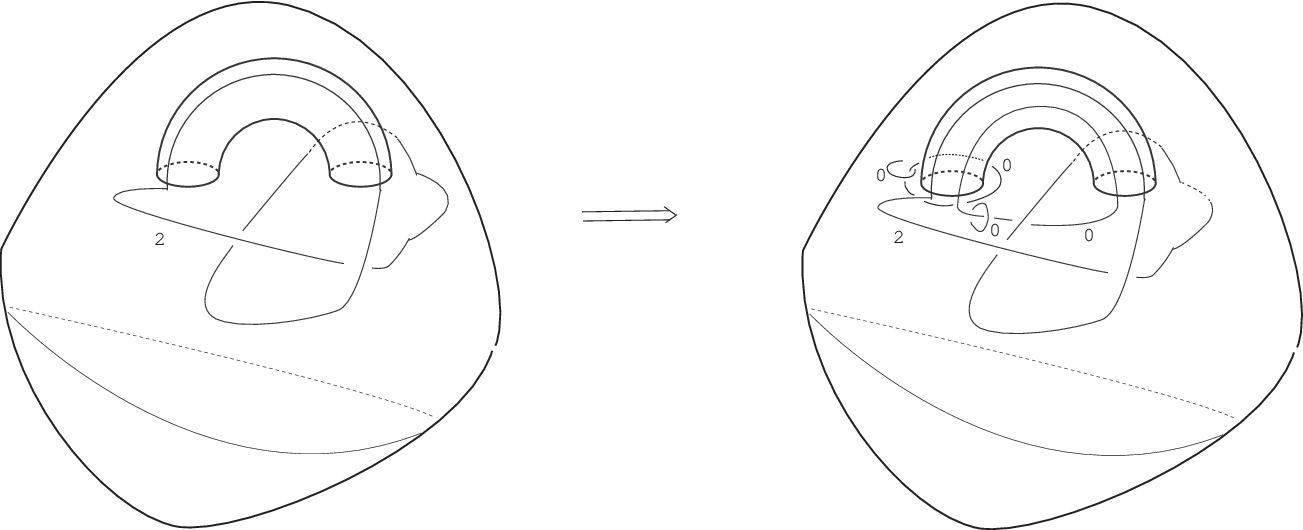
In the case of Figure 5.3, one $\mathcal{O}_{3}$ move is equivalent to a sequence of only $\mathcal{O}_{1}$ and $\mathcal{O}_{2}$ moves. Theorem 5.4 below is its generalization.

Let $F$ be a connected closed oriented surface. Let $M$ be a connected oriented compact 3-manifold with boundary $F\amalg F$ with the boundary condition $\mathcal{B}$. Let $L^{fr}$ and ${L^{fr}}^{\prime}$ be framed links in $F\times[-1,1]$ with the symplectic basis condition $\mathcal{F}$ and with the simple-connectivity condition $\mathcal{S}$, that represent $M$. By Theorem 5.3, succh framed links, $L^{fr}$ and ${L^{fr}}^{\prime}$, exist always.

Since we impose the conditions $\mathcal{B}$ and $\mathcal{F}$, we can apply Proposition 5.1 and Theorem 4.1, and claim that $L^{fr}$ is made from ${L^{fr}}^{\prime}$ by a sequence of $\mathcal{O}_{1}$, $\mathcal{O}_{2}$ and $\mathcal{O}_{3}$. Furthermore, we strengthen this fact, and obtain Theorem 5.4.

Theorem 5.4 does not follow from only Theorem 4.1. We found a new fact and proved Theorem 5.4.

By the above facts (i)-(iv) and Theorem 4.5, all $A_{i}$ satisfy the simple-connectivity condition $\mathcal{S}$. This completes the proof of Claim 5.6. ∎

The proof of Claim 5.7 is a generalization of Figure 5.3.

In Figure 5.4 we draw an example of such pair: The left hand-side and the right hand-side are examples of $X$ and $Y$, respectively. The left hand-side is changed into the right hand-side by one $+\mathcal{O}_{3}$ move. We will prove that they are changed into each other by a sequence of only $\mathcal{O}_{1}$ and $\mathcal{O}_{2}$ moves.

Take a point $P$ in $K_{L}$. Regard $P$ as the base point when we consider $\pi_{1}(F\times[-1,1])$. Take a point $P_{\ast}$ in each $X_{\ast}$. See Figure 5.5. Connect $P$ and each $P_{\ast}$ by a curved segment. This curved segment and $X_{\ast}$ make an element $\gamma_{\ast}$ of $\pi_{1}(F\times[-1,1])$ if we give an orientation.

Since $X$ satisfies the simple-connectivity condition $\mathcal{S}$, by van Kampen theorem, the elements $\gamma_{1},...,\gamma_{\xi}$ generate $\pi_{1}(F\times[-1,1])$. Hence we have the following.

Take $X$ in $F\times[-1,1]$. Take an embedded 3-ball $B$ in $F\times[-1,1]$, disjoint from $X$. By using only $\mathcal{O}_{1}$ and $\mathcal{O}_{2}$ moves, we can make a framed Hopf link $(J_{S},J_{L})$ in $B$ such that $J_{S}$ (respectively, $J_{L}$) is equipped with framing 0 (respectively, arbitrary integer).

An example of this operation: The left hand-side of Figure 5.4 is made into Figure 5.6 by using only $\mathcal{O}_{1}$ and $\mathcal{O}_{2}$ moves.

By Fact 5.8, only $\mathcal{O}_{2}$ moves (handle slices) change $J_{L}$ into a knot $J^{\prime}_{L}$ in $F\times[-1,1]$ that represents the element $[K_{L}]\in\pi_{1}(F\times[-1,1])$: If necessary, slide $J_{L}$ over $X_{\ast}$. Note that the element $[K_{L}]\in\pi_{1}(F\times[-1,1])$ was given by the assumption of Claim 5.7.

An example of this operation: Figure 5.6 is changed into Figure 5.7 by using only $\mathcal{O}_{2}$ moves.

We use only $\mathcal{O}_{2}$-moves (handle-slides): Slide $X_{\ast}$ or $J^{\prime}_{L}$ over $J_{S}$ if necessary. Thus we can move $J^{\prime}_{L}$ and let it coincide $K_{L}$ in $F\times[-1,1]$. Call $J_{S}$, $K_{S}$.

An example of this operation: Figure 5.7 is changed into the right hand-side of Figure 5.4 by using only $\mathcal{O}_{2}$ moves. Thus two framed links of Figure 5.4 are changed into each other by only $\mathcal{O}_{1}$ and $\mathcal{O}_{2}$ moves. This completes the proof of Claim 5.7. ∎

By Claims 4.7 and 5.7, we can suppose that no $\mathcal{P}_{i}$ is $+\mathcal{O}_{3}$ or $-\mathcal{O}_{3}$. This completes the proof of Theorem 5.4.∎

Kauffman [7, 9, 10] describes and develops virtual links as a diagrammatic extension of classical links, and as a representation of links embedded in thickened surfaces. The Jones polynomial of virtual links is defined in [7, 9, 10]. See related open questions in [20, §4].

We can regard any framed link in $F\times[-1,1]$ as a framed virtual link. See [3] for framed virtual links. Note that the linking number of any pair, $K_{i}$ and $K_{j}$, is defined. The value is an integer or a half integer. Note that the framing is an integer.

Quantum invariants of framed virtual links are defined there (See §8). If two framed links $L^{fr}$ and ${L^{fr}}^{\prime}$ are changed into each other by a sequence of Kirby moves ([14]) and classical and virtual Reidemeister moves, each quantum invariant of $L^{fr}$ is equivalent to that of ${L^{fr}}^{\prime}$.

We use these invariants and, will introduce quantum invariants of 3-manifolds with boundary in the following sections.

By a one-handle stabilization, we mean a surgery on the surface that is performed on a curve in the complement of the link embedding and that either increases or decreases the genus of the surface. The reader should note that knots and links in thickened surfaces can be represented by diagrams on the surface in the same sense as link diagrams drawn in the plane or on the two-sphere. From this point of view, a one handle stabilization is obtained by cutting the surface along a curve in the complement of the link diagram and capping the two new boundary curves with disks, or taking two points on the surface in the link diagram complement and cutting out two disks, and then adding a tube between them. The main point about handle stabilization is that it allows the virtual knot to be eventually placed in a least genus surface in which it can be represented. A theorem of Kuperberg [15] asserts that such minimal representations are topologically unique.

Virtual knot theory has a diagrammatic formulation. A virtual knot can be represented by a virtual knot diagram in $\mathbb{R}^{2}$ (respectively, $S^{2}$) containing a finite number of real crossings, and virtual crossings indicated by a small circle placed around the crossing point as shown in Figure 7.1. A virtual crossing is neither an over-crossing nor an under-crossing. A virtual crossing is a combinatorial structure keeping the information of the arcs of embedding going around the handles of the thickened surface in the surface representation of the virtual link.

The moves on virtual knot diagrams in $\mathbb{R}^{2}$ are generated by the usual Reidemeister moves plus the detour move. The detour move allows a segment with a consecutive sequence of virtual crossings to be excised and replaced by any other such a segment with a consecutive virtual crossings, as shown in Figure 7.2.

Virtual 1-knot diagrams $\alpha$ and $\beta$ are changed into each other by a sequence of the usual Reidemeister moves and detour moves if and only if $\alpha$ and $\beta$ are changed into each other by a sequence of all Reidemeister moves drawn in Figure 7.3.

Virtual knot and link diagrams that can be related to each other by a finite sequence of the Reidemeister and detour moves are said to be virtually equivalent or virtually isotopic.
The virtual isotopy class of a virtual knot diagram is called a virtual knot.

There is a one-to-one correspondence between the topological and the diagrammatic approach to virtual knot theory. The following theorem providing the transition between the two approaches is proved by abstract knot diagrams, see [7, 9, 10].

We can define the linking number of two components of any 2-component virtual link. See Remark 3.3 and [7, 9, 10].

[19] and its English tralslation [5] are introduction to virtual knot theory.

First, we recall the definition of the Jones-Wenzl projector (q-symmetrizer) [11]. We then define the colored Jones polynomial of a virtual link diagram. It will be clear from this definition that two equivalent virtual knot diagrams have the same colored Jones polynomial. We will use these definitions to extend the Witten-Reshetikhin-Turaev invariant to virtual link diagrams. From this construction, we conclude that two virtual link diagrams, related by a sequence of framed Reidemeister moves and virtual Reidemeister moves, have the same Witten-Reshetikhin-Turaev invariant. Finally, we will prove that the generalized Witten-Reshetikhin-Turaev invariant is unchanged by the virtual Kirby calculus. In the next section, we present two virtual knot diagrams that have fundamental group $\mathbb{Z}$ and a Witten- Reshetikhin-Turaev invariant that is not equivalent to $1$.

To form the n-cabling of a virtual knot diagram, take $n$ parallel copies of the virtual knot diagram. A single classical crossing becomes a pattern of $n^{2}$ classical crossings and a single virtual crossing becomes $n^{2}$ virtual crossings.

Let $r$ be a fixed integer such that $r\geq 2$ and let

Here is a formula used in the construction of the Jones-Wenzl projector.

Note that $\Delta_{1}=-(A^{2}+A^{-2})$, the value assigned to a simple closed curve by the bracket polynomial. There will be an an analogous interpretation of $\Delta_{n}$ which we will discuss later in this section.

We recall the definition of an n-tangle. Any two n-tangles can be multiplied by attaching the bottom n strands of one n-tangle to the upper n strands of another n-tangle. We define an n-tangle to be elementary if it contains to no classical or virtual crossings. Note that the product of any two elementary tangles is elementary. Let $I$ denote the identity n-tangle and let $U_{i}$ such that $i\in\{1,2,\dots n-1\}$ denote the n-tangles shown in figure 8.1.

By multiplying a finite set of $U_{i_{1}}U_{i_{2}}\dots U_{i_{n}}$, we can obtain any elementary n-tangle. Formal sums of the elementary tangles over $\mathbb{Z}[A,A^{-1}]$ generate the $n^{th}$ Temperly-Lieb algebra [11].

We recall that the $n^{th}$ Jones-Wenzl projector is a certain sum of all elementary $n$-tangles with coefficients in $\mathbb{C}$ [8, 11]. We denote the $n^{th}$ Jones Wenzl projector as $T_{n}$. We indicate the presence of the Jones-Wenzl projector and the n-cabling by labeling the component of the knot diagram with $n$.

We construct the Jones-Wenzl projector recursively. The $1^{st}$ Jones-Wenzl projector consists of a single strand with coefficient $1$. The is exactly one 1-tangle with no classical or virtual crossings. The $n^{th}$ Jones-Wenzl projector is constructed from the $(n-1)^{th}$ and $(n-2)^{th}$ Jones-Wenzl projectors as illustrated in figure 8.2.

We use this recursion to construct the $2^{nd}$ Jones-Wenzl projector as shown in figure 8.3.

We will refer to the Jones-Wenzl projector as the J-W projector for the remainder of this paper.

We review the properties of the J-W projector. Recall that $T_{n}$ denotes the $n^{th}$ J-W projector then

Let $K$ be a virtual link diagram with components $K_{1},K_{2}\dots K_{n}$. Fix an integer $r\geq 2$ and let $a_{1},a_{2}\dots a_{n}\in\{0,1,2,\ldots r-2\}$. Let $\bar{a}$ represent the vector $(a_{1},a_{2},\dots a_{n})$. Fix $A=e^{\frac{\pi i}{2r}}$ and $d=-A^{2}-A^{-2}$. We denote the generalized $\bar{a}$ colored Jones polynomial of $K$ as $\langle K^{\bar{a}}\rangle$. To compute $\langle K^{\bar{a}}\rangle$, we cable the component $K_{i}$ with $a_{i}$ strands and attach the $a_{i}^{th}$ J-W projector to cabled component $K_{i}$. We apply the Jones polynomial to the cabled diagram with attached J-W projectors.

The colored Jones polynomial is invariant under the framed Reidemeister moves and the virtual Reidemeister moves. This result is immediate, since the Jones polynomial is invariant under the framed Reidemeister moves and the virtual Reidemeister moves.

The generalized Witten-Reshetikhin-Turaev invariant of a virtual link diagram is a sum of colored Jones polynomials. Let $K$ be a virtual knot diagram with $n$ components. Fix an integer $r\geq 2$. We denote the unnormalized Witten-Reshetikhin Turaev invariant of $K$ as $\langle K^{\omega}\rangle$, which is shorthand for the following equation.

We define the matrix $N$ in order to construct the normalized WRT [11]. Let $N$ be the matrix defined as follows:

The normalized WRT of a virtual link diagram $K$ is denoted as $Z_{K}(r)$. Let $A=e^{\frac{\pi i}{2r}}$ and let $|k|$ denote the number of components in the virtual link diagram $K$. Then $Z_{K}(r)$ is defined by the formula

where

This normalization is chosen so that normalized WRT of the unknot with writhe zero is $1$ and the normalization is invariant under the introduction and deletion of $\pm 1$ framed unknots.

Let $\hat{U}$ be a $+1$ framed unknot. We recall that $\alpha=\mu\langle\hat{U}^{\omega}\rangle$ [11], page 146. Since $\hat{U}$ and $K$ are disjoint in $K\amalg\hat{U}$ then $\langle(K\amalg\hat{U})^{\omega}\rangle=\langle K^{\omega}\rangle\langle\hat{U}^{\omega}\rangle$. We note that $b_{+}(K\amalg\hat{U})=b_{+}(K)+1$, $b_{-}(K\amalg\hat{U})=b_{-}(K)$, and $|K\amalg\hat{U}|=|K|+1$. We compute that

As a result,

We demonstrate that the normalized, generalized WRT is invariant under the framed Reidemeister moves and the Kirby calculus. The WRT is a sum of colored Jones polynomials and it is clear that the WRT is invariant under the framed Reidemeister moves and the virtual Reidemeister moves. In particular, the normalized WRT is invariant under the first Kirby move (the introduction and deletion of $\pm 1$ framed unknots) due to the choice of normalization. We only need to show invariance under handle sliding.

By Theorem 5.4, we have the following.

Recall that the sets, $\mathcal{Y}$ and $\mathcal{Z}$, are defined below Definition 2.1.

By Main theorem 9.1 and §6, we have the following.

One can also start with a virtual diagram $K$ and associate an embedding $L$ in $F\times I$ by the reverse process. However, the resulting $L$ may not satisfy the simple connectivity condition for the associated four-manifold. One way to insure this condition is to first associate a surface to $K$ by adding a handle to the plane at each virtual crossing. Then augment $K$ at each such handle to make sure that the simple connectivity condition is satisfied. In Figure 9.1 we show how this augmentation of loops corresponds to an augmentation of a virtual diagram at a virtual crossing. Here we interpret the virtual crossing as corresponding to a handle in the surface $F.$ We illustrate the augmentation at that handle an show how it corresponds to adding virtual curves to the given virtual diagram $K$ to form a virtual diagram $K^{\prime}.$ If we start with a virtual diagram $K$ and apply this augmentation at each virtual crossing to form a virtual diagram $K^{\prime},$ then resulting diagram $K^{\prime}$ will represent a three manifold $M(K^{\prime})$ that satisfies the simple connectivity condiition. Thus the virtual Kirby class of this diagram $K^{\prime}$ will be an invariant of the manifold $M(K^{\prime}).$ In this way we can create many examples for studying the results of this paper. In Figure 9.2 we illustrate a specific example $K^{\prime}$ whose invariants can be calculated. The reader interested in seeing the details of the calculation can consult [11, 3], apply the above description of the invariants and work out the expansion of the invariants for the link $K^{\prime}$ in Figure 9.2 . We will calculate such examples in the sequel to the present paper.

Let $L$ be a 2-component 1-link in $S^{3}$. The complement has the boundary $T^{2}\amalg T^{2}$. A meridian and longitude pair is defined naturally. We can make easily a rule of how to give a handle decomposition $h^{0}\cup h^{1}_{1}\cup h^{1}_{2}\cup h^{2}$ on the boundary, $T^{2}\amalg T^{2}.$ Thus we can define surface link quantum invaraiants for the complement of the 2-component link.

Let $K$ be a 1-knot in $S^{3}$. There are many natural ways to make a 2-component 1-link from $K$:
Make a 2-component split link made from $K$ and the trivial knot.
Make a 2-component split link made from $K$ and a fixed knot.
Make a 2-component split link made from $K$ and $K$.
Make a 2-component link made of $K$ and the trivial knot $T$ so that $K$ intersects the 2-disc which bounds $T$ one time geometrically.

We can choose such a method to determine a 2-component link associated with a given knot $K$.

The complement of that 2-component link $L$ has the surface link quantum invariants described herein. By using the complement of $L$, we can define surface link quantum invariants for $K$. In this way surface link quantum invariants produce classical knot invariants. Virtual links make new quantum invariants of classical knots and links in $S^{3}$.

The surface link quantum invariants are constructed by the same surgery methods used by Reshetikhin,Turaev, Lickorish,Kauffman and Lins to produce the Witten invariant for three manifolds without boundary. We denote the invariant by $Z(M)$ just as in the original cases, but our $Z(M)$ is produced by the special surgery methods of this paper.

Note that in the case of our invariant of framed links in $F\times I,$ the value of $Z(M)$ is invariant under diffeomorphisms of $F\times I.$ This is an important property for our invariant that does not appear in the usual framework for $WRT$ invariants.

As stated in Remark 2.2, surface link quantum invariants are defined for not only closed 3-manifolds, but for 3-manifolds $M$ with boundary $F\amalg F$ with fixed handle decomposition in $\partial M=F\amalg F$. The condition on the boundary may change our invariants. It is natural from a TQFT viewpoint. In TQFT, quantum invariants of compact manifolds $M$ with boundary should not be a value, or a $1\times 1$ matrix, and should be a linear map, or a matrix, from a vector space associated with the boundary of $M$ to that. Connected with a TQFT viewpoint, we could say that the surface link quantum invaraints have the following property: Taking a different diffeormorphism map $\phi$ introduced when we define the set $\mathcal{Y}$, surface link quantum invariants could change.

The surface link quantum invariants of 3-manifolds with boundary are $SU(2)$ quantum invariants. Define $SU(n)$ quantum invariants of 3-manifolds with boundary with the boundary condition $\mathcal{B}$ for $n\geqq 3$.

References

- [1] M. Atiyah: Topological quantum field theories, Publications Mathématiques de l’IHÉS 68 (1989) 175–186.
- [2] M. Atiyah: The geometry and physics of knots, Cambridge University Press (1990).
- [3] H. A. Dye, and L. H. Kauffman: Virtual Knot Diagrams and the Witten-Reshetikhin-Turaev Invariant, arXiv:math/0407407
- [4] R. A. Fenn, and C. P. Rourke: On Kirby’s calculus of links, Topology 18 (1979), 1-15.
- [5] D. P. Ilyutko and V. O. Manturov: Virtual Knots: The State of the Art, World Scientific Publishing Co. Pte. Ltd. 2012. English translation of [19].
- [6] V. F. R. Jones: Hecke Algebra representations of braid groups and link Ann. of Math. 126 (1987) 335-388.
- [7] L. H. Kauffman: Talks at MSRI Meeting in January 1997, AMS Meeting at University of Maryland, College Park in March 1997, Isaac Newton Institute Lecture in November 1997, Knots in Hellas Meeting in Delphi, Greece in July 1998, APCTP-NANKAI Symposium on Yang-Baxter Systems, Non-Linear Models and Applications at Seoul, Korea in October 1998
- [8] L. H. Kauffman: Knots and Physics Series on Knots and Everything, Vol. 1, World Scientific 1991, 1994, 2001.
- [9] L. H. Kauffman: Virtual Knot Theory, Europ. J. Combinatorics (1999) 20, 663–691, Article No. eujc.1999.0314, Available online at http://www.idealibrary.com math/9811028 [math.GT].
- [10] L. H. Kauffman: Introduction to virtual knot theory J. Knot Theory Ramifications 21 (2012), no. 13, 1240007, 37 pp.
- [11] L. H. Kauffman and S. L. Lins: Temperly-Lieb Recoupling Theory and Invariants of 3-Manifolds Annals of Mathematics Studies, Princeton University Press (1994).
- [12] R. C. Kirby: A calculus for framed links in Invent. Math. 45 (1978), 35-56.
- [13] R. C. Kirby: The topology of 4-manifolds Lecture Notes in Math (Springer Verlag) vol. 1374, 1989
- [14] R. C. Kirby and P. Melvin: The 3-manifold invariants of Witten and Reshetikhin-Turaev for sl(2, C) Inventiones Mathematicae 105 (1991) 473–545.
- [15] G. Kuperberg: What is a virtual link? Algebr. Geom. Topol. 3 (2003) 587-591.
- [16] W. B. R. Lickorish: A representation of orientable combinatorial 3-manifolds Ann. Math. 76 (1962), 531-540.
- [17] W. B. R. Lickorish: Invariants for 3-manifolds from the combinatorics of the Jones polynomial Pacific J. Math. 149 (1991) 337-347.
- [18] W. B. R. Lickorish: Three-manifolds and the Temperley-Lieb algebra Mathematische Annalen 290 (1991) 657–670.
- [19] V. O. Manturov: Virtual Knots: The State of the Art, in Russian 2010.
- [20] E. Ogasa: An elementary introduction to Khovanov-Lipshitz-Sarkar stable homotopy type, https://www.researchgate.net/publication/352136009Anelementary introductiontoKhovanov-Lipshitz-Sarkarstablehomotopy type (The readers can find this article by typing in the title in a search engine.)
- [21] N. Reshetikhin and V. G. Turaev: Invariants of 3-manifolds via link polynomials and quantum groups, Inventiones mathematicae 103 (1991) 547–597.
- [22] N. Reshetikhin and V. G. Turaev: Ribbon Graphs and their invariants derived from quantum groups, Communications in Mathematical Physics, 127(1990) 1-26.
- [23] J. Roberts: Kirby calculus in manifolds with boundary Proceedings of 5th Gökova. Geometry-Topology Conference.21(1997)111-117, arXiv:math/9812086.
- [24] E. Witten: Quantum field theory and the Jones polynomial Comm. Math. Phys. 121 (1989) 351-399.
Louis H. Kauffman
Department of Mathematics, Statistics and Computer Science
University of Illinois at Chicago
851 South Morgan Street
Chicago, Illinois 60607-7045
USA
kauffman@uic.edu
Eiji Ogasa
Meijigakuin University, Computer Science
Yokohama, Kanagawa, 244-8539
Japan
pqr100pqr100@yahoo.co.jp
ogasa@mail1.meijigkakuin.ac.jp