Digital quantum simulation and pseudoquantum simulation of the gauge-Higgs model
Abstract
We present a quantum algorithm for digital quantum simulation of the gauge-Higgs model on a lattice, which is based on Trotter decomposition, the quantum adiabatic algorithm and its circuit realization. Then we perform a classical demonstration, dubbed a pseudoquantum simulation, on a GPU simulator. We obtain useful results on this model, which suggest the topological properties of the deconfined phase and help to clarify the phase diagram. It is suggested that the tricitical point, where the second-order critical lines of deconfinement-confinement transition and of deconfinement-Higgs transition meet, seems to be on the the first-order critical line of confinement-Higgs transition, at a point other than the end of this critical line.
I Introduction
Lattice gauge theory is a nonperturbative approach to gauge theory, especially quantum chromodynamics lgt; Kogut; Kogut2; lgtbooks; lgtbooks2. It is important not only in particle physics, but also in condensed matter physics and even in topological quantum computing S0217984914300129; toric. It is usually implemented in terms of Monte Carlo simulation, however, which lacks real-time dynamics and may suffer the well-known fermion sign problem sign; sign2; troyer; signproblem.
Recently, it has appeared that these issues may be resolved in quantum simulation reviews; reviews2; reviews3; Byrnes2006; lewenstein2; Martinez2016; Gonz_lez_Cuadra_2017; PhysRevLett.118.070501; Kasper; Kolco; lamm; Ercolessi; Gorg; Schweizer; Barbiero; Mil; Yang; Davoudi; PhysRevX.10.021041; JHEP08(2020)160; S0217979220502926; li; zhang. Moreover, as exemplified in the quantum simulation JHEP08(2020)160; S0217979220502926 of the pure gauge theory Wegner; fradkin; FradkinBook; Sachdev, for quantum simulation involving only dozens of qubits, it is very useful to make a classical demonstration on a high-performance platform, which we called a pseudoquantum simulation JHEP08(2020)160. It serves not only as a benchmark for experimental quantum simulation, which facilitates the development of quantum algorithms, but also as a new numerical method for computational problems.
We now go beyond the pure gauge theory, and consider the gauge-Higgs model PhysRevD.19.3682, where there exists coupling between matter and gauge fields, with duality between them. This model has been widely studied analytically PhysRevD.19.3682; Banks:1980gs; Gliozzi; Nussinov:2004ns; Vidal:2008uy and numerically Jongeward:1980wx; PhysRevD.21.1006; PhysRevB.82.085114; 2012.15845. Remarkably, this model is equivalent to the transverse-field toric code model PhysRevB.82.085114, which is important for topological quantum computing.
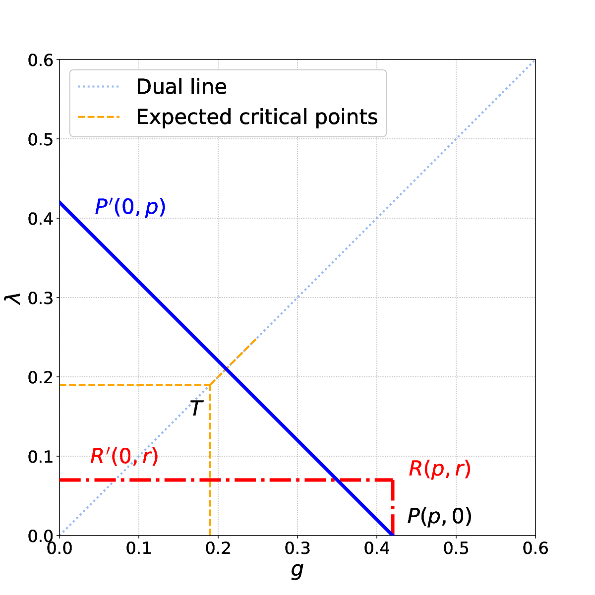
It has been known that in the gauge-Higgs model, there is a deconfined phase, separated from a confined phase on one hand, and from a so-called Higgs phase on the other (cf. Fig. 1). The phase transitions between the deconfined and the confined phases and between the deconfined and the Higgs phase are both second order, leading to a topological region surrounded by two second-order lines on the phase diagram. These two lines meet at a self-dual point. The confined and Higgs phases are separated by a finite dual line of a first-order transition, beyond which the two phases are continuously connected.
However, with strong competition between matter and gauge fields, questions such as how these critical lines are connected and where the two second-order lines meet have not been clearly answered yet, and are under debate. It has been pointed out that there are three possibilities PhysRevB.82.085114. A quantum Monte Carlo (QMC) study provides the evidence that the tricritical point, where the three critical lines meet, is scale invariant and of second order 2012.15845.
In this paper, we report a scheme of the digital quantum simulation of the gauge-Higgs model. It is digital in the sense that it is based on Trotter decomposition of the unitary evolution trotter. It uses the quantum adiabatic algorithm arXiv:quant-ph/0001106 and is implemented in terms of quantum circuits. Given that the ground state of the toric code model toric has been experimentally prepared arXiv:2104.01180, it is hopeful that our scheme can be realized in future experiments. Furthermore, we classically demonstrate our quantum simulation scheme using a GPU simulator called Quantum Exact Simulation Toolkit (QuEST) QuEST in an NVIDIA GeForce RTX 3090 GPU server. Dubbed pseudoquantum simulation, the classical demonstration of quantum simulation is also a numerical method providing useful results on this model.
We have investigated the nature of the quantum phase transitions, the adiabatic evolution along the dual line on the phase diagram, as well as the behavior near the tricritical point. Our work suggests that the tricritical point, where the two second-order lines end, lies on the line of the first-order transition, but not at the lower end of it (see Fig. 1).

The rest of the paper is arranged as follows: In Sec. II, the gauge -Higgs model is briefly introduced. In Sec. III, we elaborate on the digital quantum adiabatic algorithm and its realization in terms of quantum circuits. In Sec. IV, we describe the preparation of the initial state, as well as the topological phase. In Sec. V, we discuss the critical points according to the analysis of the density of states (DOS). The Trotter error is analyzed in Sec. VI, with some details given in the Appendix. We make a comparison between our method and exact diagonalization in Sec. VII. A summary is made in Sec. VIII.
II Model description
The Hamiltonian of the gauge-H iggs model is
| (1) |
where denotes the gauge field defined on the links, denotes the Ising matter field defined at the vertices, and
| (2) |
is the tensor product of four ’s on the sides of a plaquette . Gauss’s law requires that the ground state be invariant under the action of
| (3) |
with .
Under a mathematical mapping, the guage-Higgs model as given in Eq. (1) is equivalent to the toric code model in two transverse fields PhysRevB.82.085114, which is thus studied in this paper. We focus on the parameter subspace with . Hence the Hamiltonian reads
| (4) |
The total number of qubits is 19, with one for the ancilla and 18 for a lattice model on the torus. The size is small. Unfortunately it is very difficult to make it larger. A lattice would need 33 qubits, which is too large an increase for both the power of present classical computation and real quantum simulation in present quantum hardware, let alone even larger lattice size for the purpose of finite size scaling.
The main goal of our work is to present and classically demonstrate the scheme of the digital quantum simulation, while the calculations are a proof-of-principle demonstration shedding some light on the nature of the quantum phase transitions in this model.
III Quantum Algorithm
The purpose is to obtain the energy of the system as a function of the parameters and . Since there exists the self-duality, we only need to investigate the behavior below the self-dual line on the - parameter plane. The axis, where , represents the pure gauge theory, for which we prepare the initial ground state on a point on the axis.
Two paths of parameter variation are used for the adiabatic algorithm. As shown in Fig. 2, on a path depicted as a broken red line, the parameters vary first from to , then to . On a path depicted as a solid blue line, the parameters vary from to on the straight line.
Now, we introduce the algorithm for the digital quantum simulation, which is implemented in terms of quantum circuits and uses a quantum adiabatic algorithm to evolve the ground state along paths in the parameter space. For convenience, we write the Hamiltonian as
| (5) |
where
| (6) |
We decompose the evolution operator by using the second-order Trotter-Suzuki formula Hatano2005,
| (7) |
where
| (8) |
The decompositions in Eq. (8) do not generate errors, since the summands in commute with each other.
and can be realized simply by using the rotation gates and , respectively:
| (9) |
By introducing an ancilla , can be realized as
| (10) |
where
| (11) |
can be realized similarly, and we only need four additional Hadamard gates to switch into basis the four spins on the sides connected at —that is,
| (12) |
where
| (13) |
Note that we use the convention for the time order of the operators—that is, from right to left. We omit drawing the circuits, which is straightforward.
To ensure adiabaticity in the variation of the parameters, evolution on each path is divided into numerous tiny steps, each with the same duration of time.
IV Preparation of initial state
The initial ground state at the parameter point is the same as an intermediate state in our previous work on the pure gauge theory JHEP08(2020)160, as the mere addition of , which commutes with , does not change the state. As we have mentioned before, this has been experimentally realized arXiv:2104.01180. In our demonstration in the classical simulator, nevertheless, for convenience, we can simply use projections to prepare such a state, although it is not convenient in experiments.
The ground state is prepared from , by using
| (14) |
where P represents the projection of the ancilla to be . The idea is to first generate the equal superposition of all the computational basis states, by using a Hadamard gate on each qubit, then for each plaquette, to apply four cnot gates to transfer the information of each basis state to an ancilla JHEP08(2020)160. It leads to a superposition of all possible configurations with for every . This is a ground state at parameter point on - plane, denoted as .
Then we adiabatically evolve along the axis toward , by using the circuit-based digital quantum adiabatic algorithm in Sec. III.
If we initially prepare a ground state at by adiabatic evolution from the one at , the state prepared at should be the superposition of all configurations with for every .
The quantum circuit for preparing is
| (15) |
The ground states can be described with the aid of ’t Hooft loop operators and noncontractible Wilson loop operators , and the eigenstates of on the axis are dual to the eigenstates of on the axis FradkinBook. , , and are different eigenstates of and , with eigenvalues . As and are topological, , , , and are in different topological sectors, and a state in one topological sector cannot evolve into other topological sectors. Moreover, , , and are four degenerate ground states at .
It turns out that . Therefore, if the evolution is restricted in a topological phase, and cannot evolve to each other, because of topological protection. Hence the evolution from to should be different from the evolution from to , on the path depicted as a solid blue line in Fig. 2.
We prepare each of these two ground states on the corresponding parameter point and evolve it to the other parameter point along the solid blue path in Fig. 2. The result shows that in Fig. 3, representing the functions of the parameter , the two curves cross if the path is chosen within the deconfined phase, and they do not cross if the path is outside of the deconfined phase. The crossing here is an indication of topological phase, and it shows the irreversibility of the adiabatic evolution, which is history dependent. This feature cannot show up in exact diagonalization or QMC, which directly give results at each parameter point. Note that the crossing here is not the level crossing in a finite lattice that becomes an avoided level crossing in an infinite lattice.


V Phase diagram


We now look for the fingerprints of the critical points of quantum phase transitions as the extremal points in the second derivatives of the energy.
After numerous trials, we choose for the path depicted as the broken red line in Fig. 2, of which the value is denoted as . The result suggests that for , the critical value of is , while for , , as depicted in Fig. 4. In this way, we find that the two critical lines surrounding the deconfined phase meet at , as shown in Fig. 1.
As shown in Fig. 5, we analyze the order of the quantum phase transition by considering DOS (density of states), where the states refer to the eigenstates of , as in our previous work. When , the DOS of exhibits only one maximum in each phase. This is similar to the case of the pure gauge theory. Hence the quantum phase transition here is of second order when . This verifies that the two critical lines surrounding the deconfined phase are second order.
DOS becomes more and more disordered when , which represents the region close to the meeting point of the two second-order critical lines. Similar phenomena can also be observed on the paths in solid blue lines.


A characteristic feature of the first-order phase transition is the coexistence of different phases. As shown in Fig. 6, The conversion from single-maximal features to multimaximal features of the DOS of can be regarded as suggesting the conversion from a second-order phase transition to a first-order phase transition. However, as our system is small, although the multimaximal feature appears in DOS when in red paths, the first-order phase transition does not necessarily appear when . It is likely that it appears only after the two second-order lines cross at .
Besides, no matter what value we choose for the path of the solid blue line, we can always observe an extremal point of right on the dual line, as shown in Fig. 7. However, an extremal point does not have to be a critical point. To determine the end of the first-order phase transition line outside the deconfined phase, we need to investigate the DOS of .


Since the Higgs phase and confined phase are continuously connected when , PhysRevD.19.3682, the first-order line should vanish somewhere. Figure 6 shows the variation of the DOS on the dual line and gives two special points, and . We consider as the end of the line because the maximum at suggests that the system starts to mainly permit the excitation of the smallest loop, which is composed of four spins, while other possible configurations are generally disfavored. Consequently, the fusion of the flux and charge, which is a fermion in this model, vanishes and the system turns into confinement PhysRevB.67.245316.


Besides this, Fig. 1 suggests that there seem to be three extremal points on the paths in solid blue lines when . However, this feature can only be clearly observed when . For , we observe a single extremal point on the dual line. We regard this as a finite-size effect, which makes the extremal point on the dual line indistinguishable from the two on the second-order lines.
The extremal points on the dual line make it natural for us to study the energy right on the dual line, so we choose a new path from , through , and to . Surprisingly we find an extremal point at , which is in the deconfined phase (See Fig. 8). Moreover, the DOS is also disordered on the part of the dual line continued from the first-order line into the deconfined phase; as indicated in Fig. 5, it is likely that the first-order line extends for a range in the deconfined phase and ends at (See Fig. 1).
The phase diagram we obtain is similar to the diagram in Ref. Vidal:2008uy, which is derived by using perturbation theory. The difference lies in the extension of the first-order line in the deconfined phase. The region near the tricritical point has not been clear. Our result corresponds to one of the possibilities proposed in Ref. PhysRevB.82.085114.
VI Error analysis
As the Trotter-Suzuki decomposition is used in each step, the upper bound of the total error is a summation of the errors in each step.
We take the subpath from to as an example. As derived in the Appendix, the accumulated Trotter error is
| (16) |
where is the time for each step of varying the parameter values, and is the number of steps.
For variation of from , is the variation in each step; . We choose and , giving , which seems to be too large for us. However, this error bound is obtained by adding the absolute values of the errors in all steps, and the actual errors are not always positive and may cancel each other PRXQuantum.2.010323. We demonstrate this in the following steps.
Rewrite and , then under the parameter values above. Define
| (17) |
where is a 1-norm of the difference between two energy functions and , and represents the largest value of the difference. The results in Tabel 1 and Fig. 9 show that even when at is around 6363 times more than that at , is merely , and the maximal deviation is only . This is direct evidence that the error at each step cannot always be positive; thus, our choice of is reasonable.
| 10 | 4.58100 | 0 | 0 | ||
| 200 | 0.01145 | 0.03982 | |||
| 500 | 0.00183 | 0.04009 | |||
| 800 | 0.00072 | 0.04075 |
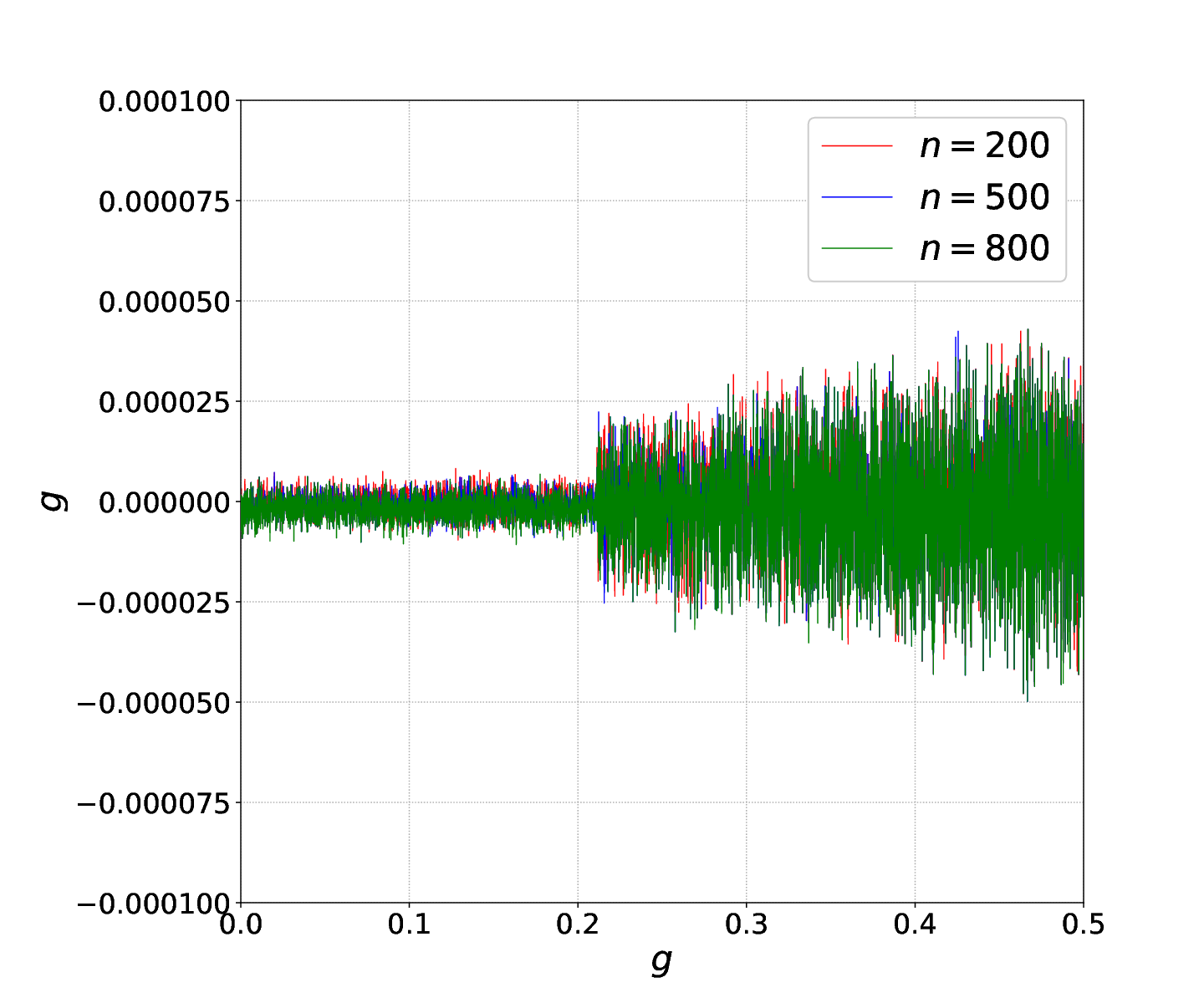
The results also demonstrate that the Trotter steps can actually be reduced in an actual quantum simulation.
VII Comparison with Exact Diagonalization
To verify the validity of our approach, we compare the results on a lattice on a torus in both exact diagonalization and our approach. We do not directly make exact diagonalization on a lattice, as it would need much more computing resources, while the scale of is close to .
For this model, exact diagonalization is more time-consuming than our approach, in which one does parallel computing with GPU. Specifically, for red paths with , the time in our approach is within 30 minutes on a single GeForce RTX 3090 for 19 qubits (complex data composed of a double data type for real components and imaginary components).
We use the same parameter values as in our model. For the evolution from to , the comparison is shown in Fig. 10. The unavoidable Trotter error and nonadiabatic error in DOS result in a difference between and , the values obtained in exact diagonalization and in our classical demonstration of digital quantum simulation, dubbed pseudoquantum simulation, respectively. However, the results on the second derivatives in the two approaches are very close to each other. As the quantum phase transition behavior is largely investigated through the second derivatives of energy, the comparison confirms the reliability of our approach.
As shown in Fig. 11, similar results can also be observed outside the deconfined phase—for example, along a blue path in blue, with .
If the evolution path passes the deconfined phase, which is topological, on a blue path with , for example, the shapes of and are quite different, as shown in Fig. 12).
For a smaller , even the shape of is clearly asymmetric, which means that the difference of on and is fairly large. The asymmetry cannot be observed in exact diagonalization or QMC.
On a lattice, as in the case of a lattice, the curves on the path from to cross that on the reverse path from to .


VIII Summary
We have designed the quantum simulation scheme of the gauge-Higgs model. The quantum simulation scheme is digital, as it is based on Trotter decomposition of the unitary evolution. It is also based on a quantum adiabatic algorithm. For each parameter value, which is varied slowly, the Trotter decomposition is used in executing the unitary transformation. Within each step in the Trotter decomposition, the unitary transformations are realized in terms of simple quantum circuits.
Moreover, as the quantum computers nowadays have not been capable of such quantum simulations, we make a thorough classical demonstration by using QuEST simulator on an NVIDIA GeForce RTX 3090 GPU server. This so-called pseudoquantum simulation not only facilitates the development of algorithms for future real quantum simulation, but is also a numerical method.
Then, we make a thorough classical demonstration by using the QuEST simulator in a NVIDIA GeForce RTX 3090 GPU server. Our demonstration is on a lattice, as limited by computational time in the pseudoquantum simulation and the number of qubits that can be realized in present quantum hardware. However, we have verified the reliability of our approach by comparing with the exact diagonalization on a lattice.
We have obtained some clear results on the topological properties of the deconfined phase, which appears useful for the solution of some open questions. In particular, our work suggests that the two lines of second-order transitions meet on the line of the first-order transition, but not on its end.
Acknowledgements.
This work was supported by the National Natural Science Foundation of China (Grant No. 12075059).APPENDIX: Calculation of the Trotter errors
It is useful to calculate and in advance where denotes the spectral norm of an operator, or the largest singular value of it. We use the estimation that , where is a Pauli operator or a tensor product of Pauli operators.

For our specific lattice model (see Fig. 13), we have
| (18) |
and
| (19) |
where the coefficient comes up due to the symmetry of the lattice. Similarly, we have and
| (20) |
Multiplying a minus sign does not change the eigenvalues of a matrix; thus, , and .
Suppose ; then, the tight error bound for the second-order decomposition is PhysRevX.11.011020
| (21) |
Our Hamiltonian is ; thus, the error bound is
| (22) |
where
| (23) |
According to Eq. (18), we have
| (24) |
and
| (25) |
The evolution in Sec. VI is from to on with increasing from to in steps. Denote ; then the total error is
| (26) |
Besides this, we have
| (27) |
References
- (1) K. G. Wilson, Phys. Rev. D 10, 2445 (1974).
- (2) J. B. Kogut, Rev. Mod. Phys. 51, 659 (1979).
- (3) J. B. Kogut, Rev. Mod. Phys. 55, 775 (1983).
- (4) M. Creutz, Quarks, Gluons, and Lattices, (Cambridge University Press, Cambridge, England, 1985).
- (5) C. Gattringer and L. Lang, Quantum Chromodynamics on the Lattice: An Introductory Presentation, Lecture Notes in Physics (Springer, Berlin, 2010).
- (6) I. Ichinose and T. Matsui, Mod. Phys. Lett. B 28, 1430012 (2014).
- (7) A. Y. Kitaev, Ann. Phys. (Amsterdam) 303, 2 (2003).
- (8) J. E. Hirsch et al., Phys. Rev. B 26, 5033 (1982).
- (9) R. Blankenbecler, D. J. Scalapino, and R. L. Sugar, Phys. . D 24, 2278 (1981).
- (10) M. Troyer and U. J. Wiese, Phys. Rev. Lett. 94, 170201 (2005).
- (11) P. Forcrand, Proc. Sci. LAT2009 (2009) 010..
- (12) U. J. Wiese, Ann. Phys. (Amsterdam) 525, 777 (2013).
- (13) E. Zohar, J. I. Cirac, and B. Reznik, Rep. Prog. Phys. 79, 014401 (2016).
- (14) M. Dalmonte and S. Montangero., Contemp. Phys. 57, 388 (2016).
- (15) T. Byrnes and Y. Yamamoto, Phys. Rev. A 73, 16 (2006).
- (16) L. Tagliacozzo, A. Celi, A. Zamoraa, and M. Lewenstein, Ann. Phys. (Amsterdam) 330, 160 (2013).
- (17) E. A. Martinez et al., Nature (London) 534, 516 (2016).
- (18) E. Zohar, D. González-Cuadra, and J. I. Cirac, New J. Phys. 19, 063038 (2017).
- (19) E. Zohar, A. Farace, B. Reznik, and J. I. Cirac, Phys. Rev. Lett. 118, 070501 (2017).
- (20) V. Kasper et al., New J. Phys. 19, 023030 (2017).
- (21) H. Lamm, S. Lawrence, and Y. Yamauchi (NuQS Collaboration), Phys. Rev. D 100, 034518 (2019).
- (22) N. Kolco, Phys. Rev. A 98, 032331 (2018).
- (23) E. Ercolessi E. et al., Phys. Rev. D 98, 074503 (2018).
- (24) F. Görg et al., Nat. Phys. 15, 1161 (2019).
- (25) C. Schweizer et al., Nat. Phys. 15, 1168 (2019).
- (26) L. Barbiero et al., Sci. Adv. 5, eaav7444 (2019).
- (27) A. Mil et al., Science 367, 1128 (2020).
- (28) B. Yang et al., Nature (London) 587, 392 (2020).
- (29) Z. Davoudi et al., Phys. Rev. Research 2, 023015 (2020).
- (30) F. M. Surace et al., Phys. Rev. X. 10, 021041 (2020).
- (31) X. Cui, Y. Shi and J. Yang, J. High Energy Phys. 08 (2020) 160..
- (32) X. Cui and Y. Shi, Int. J. Mod. Phys. B 34, 2050292 (2020).
- (33) M. Carena, H. Lamm, Y. Li, and W. Liu, Phys. Rev. D 104, 094519 (2021).
- (34) J. Zhang et al., arXiv:2108.08248.
- (35) F. J. Wegner, J. Math. Phys. 12, 2259 (1971) .
- (36) E. Fradkin and L. Susskind, Phys. Rev. D 17, 2637-2658 (1978).
- (37) E. Fradkin. Field Theories of Condensed Matter Physics, 2nd ed. (Cambridge University Press, Cambridge, England, 2013).
- (38) S. Sachdev, Rep. Prog. Phys. 82, 014001 (2019).
- (39) E. Fradkin and S. H. Shenker, Phys. Rev. D 19, 3682 (1979).
- (40) J. L. Banks and D. K. Sinclair, Phys. Rev. D 23, 2962 (1981).
- (41) F. Gliozzi and A. Rago, Phys. Rev. D 66, 074511 (2002).
- (42) Z. Nussinov, Phys. Rev. D 72 054509 (2005).
- (43) J. Vidal, S. Dusuel, and K. P. Schmidt, Phys. Rev. B 79, 033109 (2009).
- (44) G. A. Jongeward, J. D. Stack, and C. Jayaprakash, Phys. Rev. D 21, 3360 (1980).
- (45) M. Creutz, Phys. Rev. D 21, 1006 (1980).
- (46) I. S. Tupitsyn, A. Kitaev, N. V. Prokof’ev, and P. C. E. Stamp, Phys. Rev. B 82 085114 (2010).
- (47) A. M. Somoza, P. Serna, and A. Nahum, Phys. Rev. X 11, 041008 (2021).
- (48) S. Lloyd, Science, 273, 1073 (1996).
- (49) E. Farhi, J. Goldstone, S. Gutmann, and M. Sipser, arXiv:quant-ph/0001106.
- (50) K. J. Satzinger et al., Science 374, 1237 (2021).
- (51) T. Jones, A. Brown, I. Bush, and S. Benjamin, Sci. Rep. 9, 10736 (2019).
- (52) N. Hatano and M. Suzuki. Finding Exponential Product Formulas of Higher Orders, edited by A. Das and B. K. Chakrabarti (Springer, Berlin, 2005), p. 37.
- (53) M. Levin and X. Wen, Phys. Rev. B 67, 245316 (2003).
- (54) M. C. Tran, Y. Su, D. Carney, and J. M. Taylor, PRX Quantum 2, 010323 (2021).
- (55) A. M. Childs, Y. Su, M. C. Tran, N. Wiebe, and S. C. Zhu, Phys. Rev. X 11, 011020 (2021).