Road Network Evolution in the Urban and Rural United States Since 1900Preprint: APS/123-QED

Keith Burghardt Email: keithab@isi.edu Affiliation: USC Information Sciences Institute, Marina del Rey, CA 90292, USA Johannes H. Uhl Affiliation: Institute of Behavioral Science (IBS), University of Colorado Boulder, 483 UCB, Boulder, CO-80309, USA Affiliation: Cooperative Institute for Research in Environmental Sciences (CIRES), University of Colorado Boulder, 216 UCB, Boulder, CO-80309, USA Kristina Lerman Affiliation: USC Information Sciences Institute, Marina del Rey, CA 90292, USA Stefan Leyk Affiliation: Institute of Behavioral Science (IBS), University of Colorado Boulder, 483 UCB, Boulder, CO-80309, USA Affiliation: Department of Geography, University of Colorado Boulder, 260 UCB, Boulder, CO 80309, USA

August 11, 2026

Abstract

Road networks represent a key component of human settlements, such as cities, towns, and villages, that mediate pollution and congestion, as well as economic development. However, little is known about the long-term development trajectories of road networks in rural and urban settings. We leverage novel spatial data sources to reconstruct and analyze road networks in more than 850 US cities and over 2,500 US counties since 1900. Our analysis reveals significant variations in the structure of roads both within cities and across the conterminous US. Despite differences in the evolution of these networks, there are commonalities and strong geographic patterns. These results persist across the rural-urban continuum and are therefore not just a product of accelerated urban growth. These findings refine and extend existing knowledge and illuminate the need for policies for urban and rural planning including the critical assessment of new development trends.

Keywords:

Road network evolution, Urbanization, Urban systems, Network analysis, Rural-urban continuum

1 Introduction

Road networks are critical to local and (inter)national transportation and provide significant benefits to the economy, while also incurring significant construction and maintenance costs (in the hundreds of billions of US dollars) (Allen and Arkolakis 2019, Jaworski and Kitchens 2019, Fraser and Chester 2016). The costs, however, can be mitigated by well-planned and maintained road networks (Fraser and Chester 2016, Allen and Arkolakis 2019, Boeing 2019, Cervero and Kockelman 1997). The benefits of well-built road networks include greater walkability (Boeing 2019, Cervero and Kockelman 1997, Gori et al. 2014), which reduces environmental impacts, relieves public transport, increases transportation equity (Santos et al. 2008), reduces travel time (Merchán et al. 2020), and ultimately, improves city sustainability (Rao et al. 2018). It is therefore crucial to both public health and the economy to understand how the road infrastructure has evolved, so as to learn about the effectiveness of past policies based on historical data. However, historical road network data is scarce, impeding our quantitative knowledge about the past of road networks. Thus, researchers studying the longer-term evolution of road infrastructure typically rely on manually digitized road networks based on historical maps, which is labour-intensive and thus, often constrained to one or a few places (Masucci et al. 2013, Masucci et al. 2014, Kaim et al. 2020, Wang et al. 2019, Casali and Heinimann 2019). Only in recent years, larger-scale geospatial data integration efforts enabled the modeling and the analysis of historical road networks over larger spatial and temporal extents (Boeing 2020b, Barrington-Leigh and Millard-Ball 2015, Barrington-Leigh and Millard-Ball 2020). Moreover, recent work leverages large amounts of (contemporary) road network data and applies advanced statistical and network-analytic methods to study the road network characteristics of cities and other spatial entities (Boeing 2019, Boeing 2020a, Barrington-Leigh and Millard-Ball 2019, Xue et al. 2021, Badhrudeen et al. 2022). Specifically, researchers have studied how roads change over time using photography (Irwin and Bockstael 2007), integrating contemporary road network data with remote-sensing-derived data (Barrington-Leigh and Millard-Ball 2020), with historical census tract data including information on residential structures (Boeing 2020b), building construction year information (Fraser and Chester 2016), as well as cadastral parcel data containing building age information (Barrington-Leigh and Millard-Ball 2015). Such efforts are also facilitated by the availability and accessibility of detailed, and highly complete contemporary road network data for many regions of the world, such as from OpenStreetMap (Boeing 2017, Barrington-Leigh and Millard-Ball 2017). Alternatively, recent advances in computer vision and image processing enable the efficient automated extraction of historical road networks and other transportation infrastructure from historical maps, over large spatial extents (Jiao et al. 2021, Saeedimoghaddam 2020, Uhl et al. 2022, Hosseini et al. 2021). These efforts contribute to an increasing availability of data on past road networks, enabling quantitative, multi-temporal analyses of road network change over large spatial extents. In this vein, some recent work has explored the evolution of road networks in the United States (Barrington-Leigh and Millard-Ball 2015, Boeing 2020b), and at the global scale (Barrington-Leigh and Millard-Ball 2020), typically by analyzing topology-based network statistics constrained to portions of the contemporary road network attributed with a specific age estimate. These network statistics include measures of connectivity, geometric complexity, and network griddedness. While these efforts provide unprecedented insight on the long-term trends of urban road networks during the 20th century in the context of urban sprawl (Barrington-Leigh and Millard-Ball 2015) and highlight recent national-level trends (Boeing 2020b), there are a few limitations, that this study aims to address. For example, the study of (Barrington-Leigh and Millard-Ball 2015) focuses on connectivity-related aspects of road networks, and their analyses are limited to the urbanized parts of the U.S. (1990–2013), and to a subset of 10% of U.S. counties (1920–2015), respectively. The work of (Boeing 2020b) is spatially exhaustive, but has a focus on the griddedness of road networks, giving less attention to other aspects of road networks and their change over time. Thus, existing approaches on road network evolution in the U.S. are either limited in their temporal range or geographic coverage, do not account for regional variation when performing longitudinal analysis, focus on specific aspects of road networks only, and do not address scale effects, manifested in the modifiable areal unit problem (MAUP) (Openshaw and Taylor 1979, Masucci et al. 2015).

This leaves a few important gaps in our knowledge: How have U.S. road networks evolved at fine spatial scales across an extensive time window? How do these evolution patterns vary regionally, between cities, and within cities? And how do different aspects of road networks change in relation to each other? Importantly, are the trends of road network evolution stationary across the rural-urban continuum, or are these trends dependent on the degree of urbanization? The latter point addresses the general tendency for urban planning literature to focus on urban areas at the expense of understanding rural and sub-urban settlements and development (Frank and Reiss 2014). This lack of attention is unfortunate because accessibility is crucial to transportation policies, yet a focus on cities means limited knowledge of low-accessibility areas such as in periurban and rural settlements. Improving transportation equity and reducing financial hardships and pollution requires knowledge of all transportation regions including in rural settings.

We aim to address these knowledge gaps with a nearly-exhaustive exploration of road network evolution across the conterminous U.S. (CONUS) since 1900. We explore the evolution of these networks from the fine-scale intra-city level up to the inter-metropolitan level through methods such as time series clustering and feature embedding. These methods provide insights into where changes in road network characteristics occurred and how factors such as topographic constraints or heavy population increase may impact these changes. Such associations remained hidden in previous, more aggregated analysis. We find that rural and urban areas experience similar patterns, which has not been fully appreciated in earlier work, including a reduction in the gridiron structure of newer road networks, a structure associated with more walkable neighborhoods (Boeing 2019, Cervero and Kockelman 1997). These results suggest common trends, such as the popularity of the automobile, contributed to this evolution. Moreover, significant differences in evolution also arise across the U.S., possibly due to differences in topography (e.g., mountainous and flat regions) or urban planning schools of thought.

Specifically, we analyze road network data from the 2018 National Transportation Dataset (U.S. Geological Survey, National Geospatial Technical Operations Center 2018), integrated with novel, spatial data layers containing historical built-up areas and building densities since approximately 1900 (Uhl et al. 2021b, Leyk and Uhl 2018). We reconstructed historical road networks under plausible assumptions that roads were built at roughly the same time as the oldest nearby houses (see Section 2.2) (Boeing 2020b, Barrington-Leigh and Millard-Ball 2015). This integrated dataset enables us to study settlements and their changes through a road network lens at unprecedented temporal granularity and spatial resolution (Leyk et al. 2020, Uhl et al. 2021a). From these networks, containing in total over nine million nodes and over fifteen million road segments, we extract several road network statistics, such as the mean degree (the number of roads at each intersection), road density (the kilometers of road per unit area), a local griddedness metric, and the orientation entropy of road segments (Boeing 2019, Boeing 2021), among others. These statistics can be used to quantify key characteristics of development within spatial units of different granularity (e.g., metropolitan areas, counties, grid cells).

2 Data & Methods

2.1 Data

Herein, we use geospatial vector data from the United States Geological Survey (USGS) National Transportation Dataset (U.S. Geological Survey, National Geospatial Technical Operations Center 2018), representing the US road network in approximately 2018. We model retrospective extents of built-up land with the Historical Settlement Data Compilation for the U.S. (HISDAC-US; (Uhl et al. 2021b, Leyk and Uhl 2018)), which are derived from parcel-level built-year information contained in Zillow’s Transaction and Assessment Database (ZTRAX; (Zillow Inc. 2016)). More specifically, we use historical built-up areas (BUA) which are available in 5-year intervals from 1810 to 2016 as a series of binary, gridded surfaces at a resolution of 250m ((Uhl and Leyk 2020a), Figs. 1 & 2a). Likewise, we use historical estimates of the number of buildings per grid cell (built-up property locations; BUPL, Fig. 1 & 2b) (Uhl and Leyk 2020b), as well as the First built-up year (FBUY), mapping the earliest year of development per grid cell (Leyk and Uhl 2018, Uhl et al. 2021b) (See Fig. 1). While HISDAC-US data coverage is sparse in some rural areas of the US, geographic coverage and temporal information is largely complete in urban regions (Uhl et al. 2021b), which we discuss in more detail in Section 3.4. Moreover, the accuracy of the built-up extents layer increases over time (Leyk and Uhl 2018, Uhl et al. 2021b), reaching acceptable levels after 1900 (Uhl et al. 2021b). Thus, we constrain our analysis to the time period from 1900 to 2010. To measure road network characteristics for individual cities, we use the metropolitan statistical areas (MSAs) and micropolitan statistical areas ( $\mu$ SAs), defined by the US Office of Management and Budget, which allows results to be compared against previous work (Barrington-Leigh and Millard-Ball 2015, Boeing 2020b). Collectively, these are known as Core-Based Statistical Areas (CBSAs) and roughly delineate cities based on the commuting patterns in their surroundings (Census Bureau 2015). MSA and $\mu$ SA boundaries are shown in Supplementary Fig. S1. CBSAs nest within US county boundaries (Census Bureau 2021). Counties are also employed in this study to model road network trends across the rural-urban continuum, using county-level rural-urban continuum codes (RUCC) provided by the US Department of Agriculture (USDA 2021), classifying each county into one of nine levels of “rurality” (Supplementary Fig. S1).

Refer to caption — Figure 1: Input datasets and workflow of the three analytical components of this analysis at the CBSA, county, and grid-cell level.

2.2 Methods

Based on the various datasets, we develop a three-part analysis, aiming to assess long-term road network evolution at three different levels of spatial granularity including the analysis of (a) urban road networks at the city level, within CBSA boundaries, (b) road networks in urban, peri-urban and rural settings at the county-level, grouping them into strata of “rurality” by means of the county-level RUCC, and (c) intra-urban, local road network characteristics at the grid-cell level within CBSA boundaries.

2.2.1 Historical urban road network modeling

We make a reasonable assumption that road networks remain unchanged in their geometry, once they are established (Scheer 2001), and that the evolution of road networks is largely characterized by expansion over time, and, to a lesser degree, by densification, which is in line with assumptions in previous work (Boeing 2020b, Barrington-Leigh and Millard-Ball 2015, Meijer et al. 2018), due to the rarity of road network shrinkage. Changes in the geometric structure (e.g., layout, orientation) of road networks, or shrinkage are rare, and are assumed to be negligible in the case of the US during our study period. Thus, multi-temporal spatial data measuring the expansion of developed, or built-up land over time is commonly used to spatially constrain contemporary road networks to their assumed historical extents, under the assumption that the year of earliest settlement roughly corresponds to the year when nearby roads have been constructed (Boeing 2020b, Barrington-Leigh and Millard-Ball 2015, Barrington-Leigh and Millard-Ball 2020, Fraser and Chester 2016).

Based on the gridded surface series BUA and BUPL from the HISDAC-US we develop an approach to generate spatially generalized urban extents, consistent across different cities and over time. In a first step, we generate a built-up density surface for each half-decade from 1900 – 2010, within each 2010 CBSA boundary. To do so, we use circular focal windows of radius $r=1$ kilometer, containing the proportion of built-up area within the focal neighborhood, derived from the BUA surfaces (Fig. 2a). We then select all grid cells with a focal built-up density greater than 5%. This method has previously been employed to discretize the rural-urban continuum into high density (urban) and lower density (peri-urban) strata (Leyk et al. 2018) and shows high discriminative power between signals in remotely sensed spectral responses in urban settings. For each CBSA and year, we then segment the resulting contiguous groups (“patches”) of urban grid cells and compute the sums of built-up area, and number of buildings per patch (from the underlying BUPL surface, Fig. 2b). We then compute the percentile ranks of the patches within a CBSA according to the number of buildings they contain. We discard small patches containing less than 10 buildings, likely representing scattered peri-urban settlements. To do so, we only retain patches that exceed the 90th percentile in the first year when the density filtering yields at least one patch of built-up land (which may be later than 1910 for late-developing cities). This way, we ensure that urban areas are modelled based on consistent criteria across space and time, and represented by smooth, contiguous, and largely gap-free areas (Fig. 2c). We then clip the NTD road vector data to the urban delineations in each year, yielding sub-networks that can be uniquely identified by the combination of CBSA and year. We therefore model the intra-urban road networks for each CBSA and year, consisting of a total of 8 million nodes and over 10 million edges within CBSAs, as a basis to calculate a range of road network metrics (Section 2.2.4).

A detailed example of the reconstructed intra-urban road network is shown in Figs. 2 & 3a-c. Besides these binary data, we also attribute the road age estimate to each road network segment. The evolution of a subsection of the metropolitan area can be seen in Fig. 3d, with lighter colors denoting older roads, and darker colors representing newer ones.

2.2.2 CONUS-wide historical road network modeling

While the urban street networks we model in Section 2.2.1 allow us to characterize road network trends for large cities (metropolitan areas) and medium-size cities (micropolitan areas) over time, they do not cover the full urban-rural continuum, and are based on cumulative rather than incremental areal extents. To derive trends of road network characteristics over time and across the rural-urban continuum, we use the 2018 NTD road network vector data (U.S. Geological Survey, National Geospatial Technical Operations Center 2018, USDA 2021) and the first built-up year dataset (FBUY), from the HISDAC-US data repository (Leyk and Uhl 2018, Uhl et al. 2021b). We first identify grid cells developed within moving temporal windows (i.e., time periods) of 40 years, shifted in steps of 20 years, e.g., developed prior to 1900, 1880-1920, 1900-1940, 1920-1960, etc., as shown in Fig. 4. This is done to generate smooth trends avoiding abrupt changes in the extracted road network metric time series. For each county in the CONUS, we then extract the road network vector objects within the areas corresponding to each 40-year development period and assign an individual identifier to each contiguous group of developed grid cells (patches). We remove small, spatially isolated patches of under 0.31 square kilometers (corresponding to five 250 by 250 meter grid cells), as well as elongated patches of less than 500 meter width, likely representing settlements along highways and thus not relevant for characterizing road networks in cities, towns, or places (see Fig. 1 and Supplementary Fig. S2). For the remaining patches, containing over 27 million road segments, we calculate a range of road network metrics (see Section 2.2.4), aggregated per county and year. We analyze each of the network metrics in a bi-variate manner over time and across the rural-urban continuum, stratified by US census region (Census Bureau 2018), where the rural-urban continuum is based on the county-level rural-urban continuum codes (RUCC) provided by the US Department of Agriculture (USDA 2021), that classifies each county into one of nine levels of “rurality.” In total, we analyze 9.2 million nodes and 15.2 million edges across the rural-urban continuum. Both CONUS-wide and CBSA level historical road networks are extracted using ESRI ArcPy (ArcGIS 2021) and Safe Software Feature Manipulation Engine Desktop (Software 2021).

2.2.3 Gridded surfaces of road network metrics

The road networks we extract in Sections 2.2.1 and 2.2.2 allow for the derivation of multi-temporal, road network statistics aggregated to the CBSA- and county-level. While these aggregation levels are expected to facilitate the quantification of trends across regional strata, or strata of different levels of rurality, they may ignore fine-grained spatial variations of road network characteristics within urban areas. Thus, we use grid cells of $1\times 1$ kilometer as a third analytical unit for this study.

Using the FBUY gridded surface from HISDAC-US (Uhl et al. 2021b, Leyk and Uhl 2018), we calculate the average settlement age within $1\times 1$ kilometer grid cells located within the 2015 urban delineations derived from the density-based delineation method described above using GeoPandas (Jordahl et al. 2020) and SciPy (Virtanen et al. 2020)) Python modules. The aggregation to $1\times 1$ kilometer grid cells aims to avoid small sample sizes of road segments and intersections per grid cell, and thus, ensures the statistical support for the network statistics calculated per grid cell. We then identify all network nodes within a grid cell, as well as the centroids of all road segments (i.e., network edges) per grid cell. We calculate road network statistics for each grid cell based on the network statistics attributed to each node and to each edge (see Section 2.2.4). For consistency with the aggregated CBSA-level analysis, we calculate these grid-cell level statistics within the density-based generalized urban area from 2015 only (see Section 2.2.1).

Road network metric	Unit	Aggregated analytical unit	Description
Degree	Node	grid cell, county, CBSA (average)	Number of roads touching a node
Local griddedness	Node	grid cell, CBSA (average)	Number of quadrilaterals touching a node divided by its degree
Road density	Edge	Grid cell, county, CBSA	km road per km built-up area
Orientation entropy	Edge	County, CBSA	Entropy of edge orientation angles, discretized into bins of $5^{\circ}$
Azimuth variety	Edge	Grid cell	Number of unique edge orientation angles, discretized into bins of $5^{\circ}$
Dead end rate	Node	Grid cell	Percentage of nodes of degree 1
Nodes per km road	Node/edge	Grid cell	Number of nodes per km road within spatial unit
Node density	Node	Grid cell	Number of nodes within spatial unit
Percentage degree 4+	Node	CBSA	Percentage of nodes with degree 4 or higher
Road distance (total km road)	Edge	CBSA	Total km road within spatial unit
Straight road rate	Street	County	Percentage of streets (i.e., edges with the same street identifier) with a edge orientation standard deviation $<10^{\circ}$

Table 1: Road network metrics used in this study.

2.2.4 Road network metrics

For the historical road networks extracted per CBSA and year (Section 2.2.1) per county and development period (Section 2.2.2), and per $1\times 1$ km grid cell within CBSAs, we calculate a range of road network metrics (Table 1). These metrics include the mean degree (the number of roads at each intersection), road density (the kilometers of road per unit area), measures of road network orientation (orientation entropy, azimuth variety), and several aggregated statistics, such as node density, nodes per km road, total road distance, the dead end rate, as well as a novel local griddedness metric. Many of these statistics are based on topology, but because the majority of junctions are straight there is less need to focus on non-trivial paths between intersections. This should not affect most metrics except entropy (which could be affected by non-trivial interactions with degree-two intersections) or griddedness metric, as we explain below. We use 1 km square grids to capture these statistics because less than 0.01% of roads within CBSA boundaries are longer than 1 km.

Griddedness has become critical to understanding walkability and related problems for cities in the US but measuring it has been difficult until recently. Namely, grid-like road networks appear to enhance walkability and lower relative vehicular travel in a city (Boeing 2020b, Cervero and Kockelman 1997). Griddedness (and related urban sprawl) metrics have been defined and implemented on several recent occasions (Boeing 2020b, Barrington-Leigh and Millard-Ball 2019, Barrington-Leigh and Millard-Ball 2020). The methods to derive such metrics are sophisticated (Boeing 2020b) and sometimes computationally expensive (Barrington-Leigh and Millard-Ball 2019, Barrington-Leigh and Millard-Ball 2020). However, we aim for a simple, intersection-level measure to extend on previous work.

We develop the local griddedness metric, a spatial complement to the clustering coefficient often used in network analysis (Watts and Strogatz 1998, Boeing 2020a, Boeing 2021). The local clustering coefficient of a node is defined as the proportion of triangles that exist whose vertex includes that node relative to the total number of possible triangles that could exist for a node of that degree. Unlike, e.g., social networks, road networks tend to be quadrilaterals, and more uniquely still, these cycles tend to be planar, meaning they all lie on a two-dimensional plane.

These constraints offer guidance to a unique spatial clustering coefficient, local griddedness, which is the proportion of four-cycles containing that vertex relative to the total number of planar four-cycles for a node with that degree. Degree one, two, and three nodes are common and special cases for intersections, however. If a node is the end of a dead-end road, we define the local griddedness to be zero. We do not analyze nodes of degree two, because these nodes represent the continuation of a road, rather than an intersection. We show examples of this and explain our justification in more detail in the Supplementary Fig. S3. Finally, it is unlikely for a three-road intersection to have three city blocks meet there, but more likely is that it ends in a “T.” The maximum number of city blocks is therefore defined as two and is otherwise the degree. While in most cases, local griddedness is between 0 and 1, we allow for rare instances in which, for example, degree-three nodes have a value up to 3/2 (a “super gridded” node), for the T intersection to have a natural griddedness value of 1.0. This also means that roads that violate this planar assumption (e.g., those with bridges) may be greater than 1, but such instances are rare. Using this measure, any node can have its griddedness value rapidly calculated, allowing for extremely fine-grained analysis of road network spatial statistics.

Because this metric is based on the road network topology, a limitation of this technique is that some nodes can be misidentified as having a high griddedness value, although this is rare from visual inspection. Topology is useful both because it appears reasonable and is very fast, which partly motivates its use in, e.g., (Figueiredo and Amorim 2007, Caldarelli et al. 2004). Our method differs from previous work because it is node-centered, instead of edge-centered (Figueiredo and Amorim 2007), and is normalized such that values near 1.0 are irongrid-like, while some similar metrics are not as easy to interpret (Caldarelli et al. 2004).

In addition to this metric, we separately calculate azimuth variety and orientation entropy by binning the angles between road intersections into six-degree wide bins. Changing the width of the bins does not qualitatively change our findings but can change the absolute value of entropy (which can be as high as the log of the number of bins) as well as the azimuth variety.

Finally, we quantify the proportion of cul-de-sacs (i.e., the dead end rate). This metric requires that end points of the road vector lines that are introduced by the clipping are recorded and excluded from subsequent node analysis because these nodes represent artificial cul-de-sacs introduced by the data processing that would yield inflated dead end rate values. The road network metrics at CBSA and grid cell level are computed using NetworkX, and the statistics per development period and county are obtained using Safe Software Feature Manipulation Engine.

Figure 5 demonstrates how these statistics reveal interesting differences in road network structure between, as well as within, metropolitan areas. For example, azimuth variety (i.e., the variety of unique road orientation angles) is high (representing very irregularly oriented roads) in the Baltimore Washington area and low (regular roads) in the periphery of the Denver and Los Angeles metropolitan areas. Similarly, strong variations can be seen for the local griddedness metric. We observe in Fig. 5 low local griddedness (fewer square blocks) and low edge density (spaced out roads)in some areas of the metropolitan areas of Los Angeles, Washington DC, and Denver where newer roads were built.

2.2.5 Metropolitan-level historical road network statistical analysis

To construct CBSA-level analyses of the road networks, we group the patches constructed in Section 2.2.1 into CBSA regions. If a patch is on the border of a CBSA region, we cut it off at the boundary, and edges that reach the boundary are removed; this is not common but is a reasonable way of defining patches associated with only one metropolitan or micropolitan area. At ten-year intervals between 1900 and 2010, as well as for 2015, we construct the road network topology using the Python library NetworkX, and remove nodes with degree two from the analysis, which we explain in more detail in Section 2.2.3 and Supplementary Fig. S3. For each CBSA, we record the total road length, area, degree, proportion dead ends and degree greater than or equal to four, as well as orientation entropy and local griddedness. These raw statistics are used to construct combined measures, e.g., the distance per unit area to be able to quantify the road length distance within all patch areas (which are a small proportion of the total CBSA area).

2.2.6 Grid-cell-level correlation analysis and time series clustering

In total, we calculate seven grid cell-level network statistics (cf. Table 1). Due to potentially small sample sizes within grid cells, we replace the orientation entropy by the variety of unique azimuth values per grid cell, calculated after discretizing the road segment azimuth into bins of ten angular degrees. Based on the gridded surface indicating the average age per grid cell, and corresponding cell-level network statistics within each CBSA, we extract cell-by-cell pairs of settlement age and road network statistics for each city. These vectors enable us to calculate correlations between age and network characteristics, for each city, considering the local, fine-grained variability of settlement age as it is associated with the characteristics of the road network. Moreover, we generate time series of each network characteristic for each city. To characterize the relative relationship between age and network characteristics, we discretize the age surface per CBSA into deciles. Thus, the resulting time series consists of the same number of observations (i.e., ten) and are independent from the absolute age of the cities. For each of the network characteristics, we conduct time series-based cluster analysis separately for MSAs and $\mu$ SA. We use the time-series $k$ -means algorithm, TSK-means (Huang et al. 2016), in conjunction with the Dynamic Time Warping (Müller 2007) similarity metric to characterize the dissimilarity between time series, implemented in the tslearn (Tavenard et al. 2020) Python module. In order to identify the optimum number of clusters $k$ , we calculate the cluster inertia based on DTW similarity as a measure of separation between time series clusters for a range of $k$ from two to twenty and use the popular elbow method (Syakur et al. 2018) to identify the approximate number of clusters for each scenario. We normalize the cluster inertia of each clustering scenario into the range (0, 1) to compare the cluster quality across the different network statistics. Moreover, we assess the agreement of the CBSA clusters identified for different road network metrics using Normalized Mutual Information (NMI) (Forbes 1995).

3 Results

We carry out longitudinal and cross-sectional studies of the evolution of the US road networks since 1900, at spatial scales ranging from the grid cell level to the CONUS. Firstly, we present regional trends of urban road network evolution (Section 3.1), and identify types of city-level road network evolution (Section 3.2). Finally, we present the county-level trends of road network evolution across different development periods and across the rural-urban continuum (Section 3.3).

We begin our analysis on CBSA-level trends.

3.1 Regional trends of road network evolution

At the national level, Fig. 6 reveals broad trends in how road density varies across U.S. census regions ((Census Bureau 2018); henceforth referred to as regions). We find relatively low road density in the Midwest as well as the Northeast although the distribution in the Northeast shows a pronounced broad tail due in large part to the New York City MSA (Fig. 6a). The mean degree (i.e., mean number of roads per intersection) of networks, in contrast, is typically higher in the Midwest and lowest in the more mountainous regions (e.g., the Appalachian Mountains) near the East coast (Fig. 3b). In agreement with these statistics, we find that orientation entropy, a proxy of the road network’s regularity, is lowest (most regular) in the Midwest and highest (least regular) in the South and Appalachia. Complementing these observations, local griddedness and mean degree are highest in the Midwest and lowest in the South and mountainous regions in the West. Our temporal analysis, meanwhile, reveals that across 115 years some regions, such as the South and West, have seen great changes in their road networks, while the Northeast has been relatively stable due to limited additions of new roads in an already developed region (see Fig. 6c and Supplementary Fig. S4). In general, however, newer road networks tend to be less grid-like and less densely packed as they expanded into suburban areas (Fig. 3).

3.2 The evolution of road networks at the city-level

Fig. 7 illustrates the evolution of road networks within metropolitan areas based on network statistics extracted for each $1\times 1$ kilometer grid cell, since the first recorded building was constructed. For this analysis, we use several metrics including the ratio of dead end roads, the number of intersections per kilometer of road, the number of nodes, and length of road per area unit, and mean degree. We assess correlation of these metrics with the age of each grid cell, as shown in Fig. 7a (temporal correlations for all metrics are shown in Supplementary Figs. S5 & S6). Broadly speaking, density and griddedness-related metrics decrease over time, while azimuth variety shows mixed trends during the study period, and the dead end rate increases with road network age. These trends are similar for large cities (MSAs) and smaller cities ( $\mu$ SAs; see Supplementary Fig. S6). Figure 7b–c shows the spatial distributions of correlation coefficients between age and the two metrics azimuth variety and local griddedness, respectively, revealing strong spatial patterns. We try capturing this spatial variation by computing k-means clusters of temporal patterns in these statistics (Huang et al. 2016). We measure similarity between the time series of the CBSAs using the Dynamic Time Warping (DTW) distance metric (Müller 2007). This metric yields large distances for time series that differ considerably in their trend, shape, and/or timing. We find the data series can be grouped well into just 3 clusters (for MSAs), and 4 clusters (for $\mu$ SAs), as indicated by the “elbow” in the DTW-based cluster inertia in Supplementary Fig. S8. We separately analyze MSAs and $\mu$ SAs to understand how their evolution is affected by the size of the urban area, as CBSAs of similar age can evolve very differently. The agreement of these CBSA clusters based on individual road network metrics (measured by the Normalized Mutual Information (NMI) (Forbes 1995) varies between metrics, but is consistent across MSAs and $\mu$ SAs (Fig. 7d). High NMI values as observed for pairs of metrics such as mean degree and local griddedness indicate that CBSAs are separated into clusters in a similar manner, indicating that the temporal trajectories of the road network griddedness and mean degree follow similar evolution types. When mapping the computed clusters as shown in Fig. 7e–f, we find that the identified “types” of road network evolution at the city level follow strong spatial patterns. For example, we find that nearby cities in the Appalachian region or in the Northeast have similar trends in their azimuth variety. These results reveal a Simpson’s paradox (Simpson 1951) in that the trends in disaggregated data differ from the overall trends shown in Supplementary Fig. S7 and in previous work (Boeing 2020b, Barrington-Leigh and Millard-Ball 2015). Griddedness trajectories for MSAs, however, are distinct between the East and the West. The temporal patterns for these clusters are shown in Fig. 7g–h, where azimuth variety grows fast in MSAs of clusters 1,2, and 3, and decreases for cluster 4 (roughly covering Appalachia and the Northeast) where starting values were highest. In contrast, griddedness in MSAs decreases most in cluster 4 (West, Midwest) where values are highest and slower elsewhere (including the coastal regions). The clustering results for all seven grid-cell level statistics are shown in Supplementary Fig. S8.

While these univariate trends provide interesting insight, how do metrics for each city vary over time? The multivariate trajectories of CBSA-level network statistics over time are visualized in Fig. 8a, where we embed statistics for each city into two dimensions using UMAP (McInnes et al. 2018). UMAP is a more nuanced version of PCA embedding, where in this lower-dimensional space the relative position of datapoints are approximately preserved. The embeddings are based on seven statistics computed for each CBSA and smoothed over time: the proportion of dead ends, mean degree, road distance per area, log of road distance, local griddedness and entropy (Boeing 2019), and proportion of intersections with four or more roads (details on data smoothing are seen in Supplementary Figs. S9 & S10). Changes in statistics are highlighted by radar charts computed for the Chicago, Washington, DC, Boston, and Denver MSAs. In Fig. 8c, we also show how these statistics vary across the UMAP projection, thus providing insight into the trends of individual cities, in a way similar to Badhrudeen et al., (Badhrudeen et al. 2022). Our results demonstrate broad similarities but also considerable variation in city-level trends over time. Cities across but also within regions differ in their routes to their final statistics, yet again pointing to Simpson’s paradox in our data: trajectories, disaggregated to the level of a metropolitan region can differ, sometimes substantially, from any assumed overall trend, regionally or nationally. Nonetheless, we see some trends are consistent across cities, as shown in Fig. 8b, such as lower road density, fewer roads per intersection, and statistics consistent with less gridiron-like roads (although orientation entropy has recently started to decrease, possibly implying more regular angles between intersections). Results are robust to data cleaning (Supplementary Fig. S7). These plots illustrate the heterogeneity in the evolution of cities that resulted in today’s urban areas of the US.

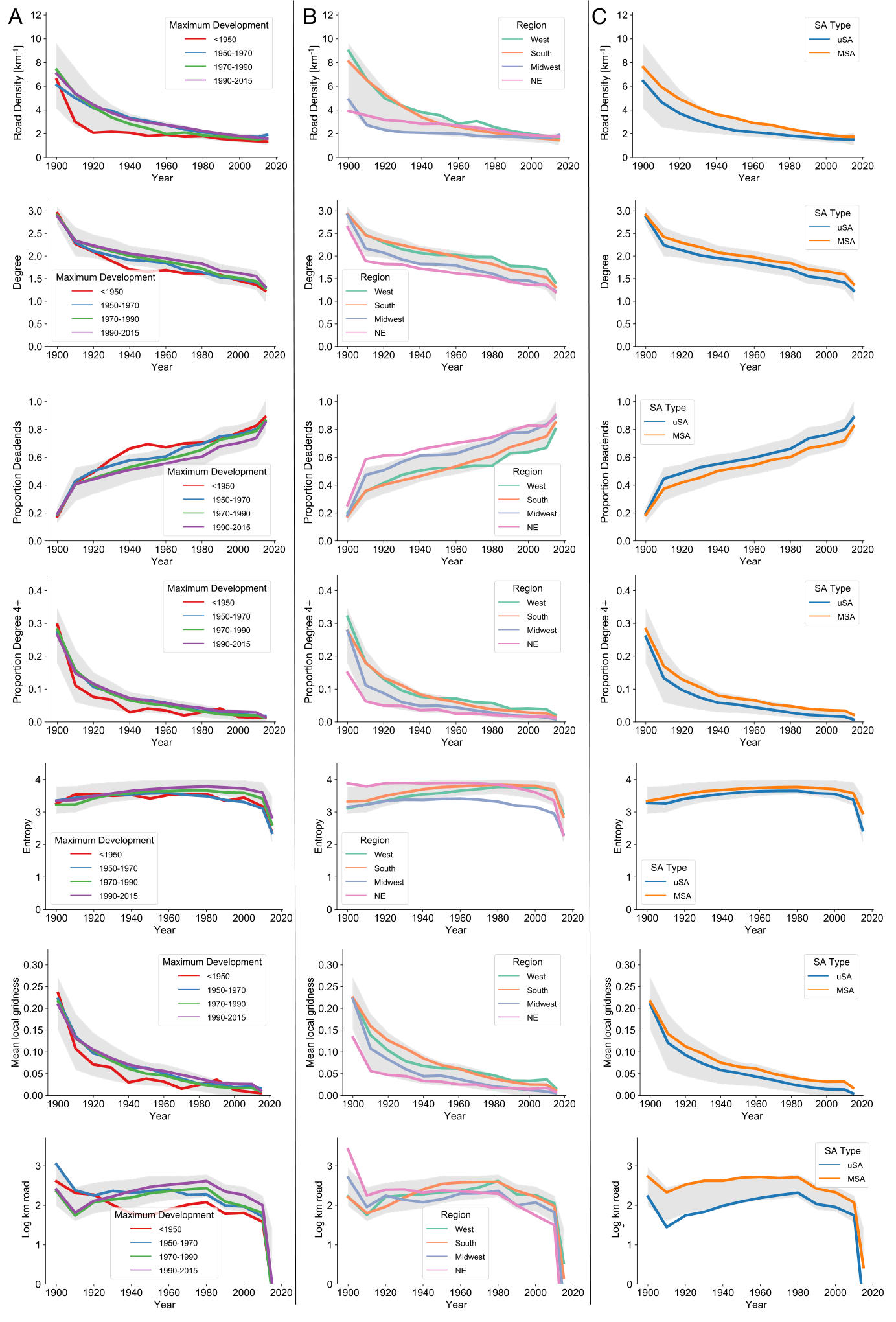
Figure 8b, meanwhile, reveals changes in road network statistics over time. There are general trends of increasing entropy and decreasing road density and griddedness across the CONUS. We observe significant variance in the computed statistics across cities in early times, especially with road density and local griddedness. However, there are also notable commonalities, such as a tendency for newer regions to have lower griddedness and higher entropy (although entropy’s trend is non-linear). The trends for mean degree and mean griddedness reveal decreasingly grid-like networks over time (statistical significance of results are shown in Supplementary Fig. S11). While scholars have argued that grid structures enable efficient traffic flows and thus, may contribute to reduce emissions, congestion, and to increase the use of alternative, environmentally friendly transportation methods (Boeing 2019, Boeing 2020b, Cervero and Kockelman 1997, Sharifi 2019, Gao et al. 2013), more recently developed road networks appear to be less effective in that regard. But why? Some trends may be due to urbanization expanding into hilly topographies, such as in the mountains north of downtown Los Angeles or the Piedmont region of western Maryland (see Fig. 2), where grid-like road networks and high road densities are not feasible. Residential development in these topographically more complex areas but also altered development patterns in periurban areas may help explain the decline in urban densities (Gao et al. 2013, Angel et al. 2017), but future work needs to analyze these hypotheses in greater detail.

3.3 Road networks across the rural-urban continuum

Finally, we analyzed and compared trends along the full rural-urban continuum (including counties outside of the CBSAs), using county-level rural-urban classes (USDA 2021), stratified by regions (rural-urban continuum values for each county are shown in Supplementary Fig. S1). While significant insight has been gleaned from analysis of urban road network growth (Barrington-Leigh and Millard-Ball 2015, Boeing 2020b), Fig. 9 reveals its complement, road network growth in periurban and rural settlements. These results demonstrate that our findings generalize to rural areas. Namely, the mean degree, road density, and straight road rate in developed areas within rural and urban settings are all decreasing from 1900 to 2015 across all regions within the CONUS. Differences in statistics across the rural-urban continuum are often, however, statistically significant (Supplementary Fig. S11 & S12). Trends vary most for orientation entropy, which tends to increase in urban settlements, but is stagnant and low in rural settlements. Comparing the road networks established in a fixed time across the rural-urban continuum, we observe high levels of persistence, indicating similar road construction trends in urban and rural places in a given time period. One notable exception are rural settlements in the Midwest, which initially have a higher road density than urban settlements, but this reverses for roads built in more recent time periods, and therefore looks more like the rest of the US.

While we focus on rural and urban trends in this section, the observed trends are also consistent when split by MSA or $\mu$ SA, region, or year of city’s maximum development (see relation between maximum development year and regions in Supplementary Fig. S13), with some minor differences, as shown in Supplementary Fig. S14.

3.4 Uncertainty, validation and sensitivity analysis

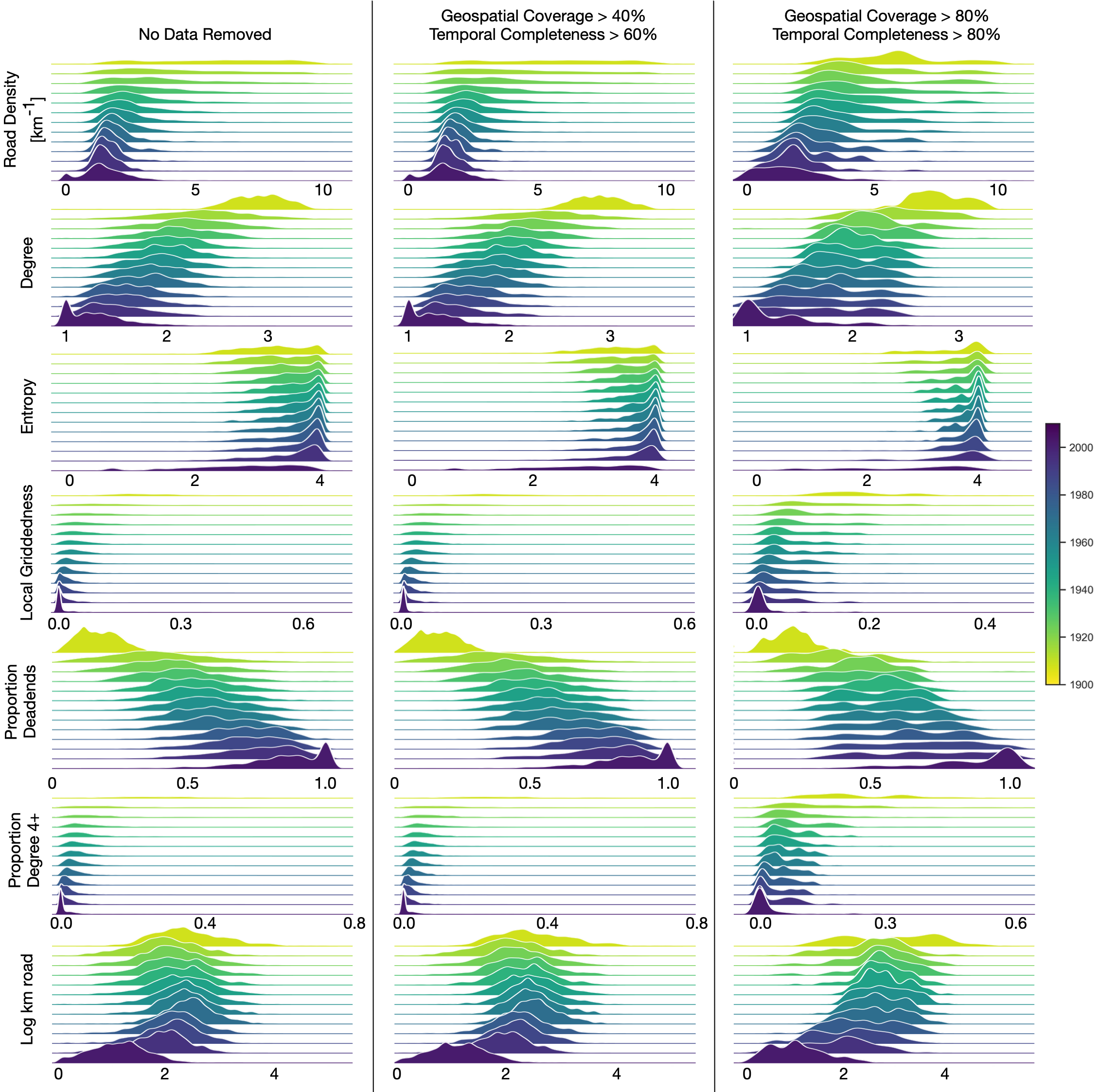
While the HISDAC-US data provides accurate building ages across the US, these data are incomplete. More specifically, many buildings are missing their build year (temporal incompleteness) and some are missing from the dataset entirely (incomplete geographic coverage). We quantified the geographic coverage by comparing the buildings found against the Microsoft Building Footprint dataset (Microsoft 2020), and the temporal completeness by quantifying the availability of YearBuilt in ZTRAX (Supplementary Figs. S15 & S16). We also assessed the sensitivity of our main results to different levels of completeness, by systematically excluding CBSAs of lower completeness levels. Our findings are robust to such variations in data quality (see Supplementary Figs. S17, & S18).

To further verify our results, we compare some of our findings to previous work (Boeing 2020b, Boeing 2020a, Barrington-Leigh and Millard-Ball 2015). We compare differences in statistics between small and large cities (Supplementary Fig. S19) and regional network statistics (Supplementary Fig. S20), as well as trends based on most statistics, such as mean degree or dead-end rate (Supplementary Figs. S21), and all statistics in the present study broadly agree with previous research. However, in contrast with recent research (Boeing 2020b, Barrington-Leigh and Millard-Ball 2015), we did not find a significant increase in mean degree or proportion of four-way intersections in the 21st century. Some of these results are likely data-dependent (Barrington-Leigh and Millard-Ball 2015) but some observed differences may also be due to the MAUP (Openshaw and Taylor 1979, Masucci et al. 2015). Our large dataset allows us to analyze historical road networks, which are reconstructed based on the age information of nearby settlements, at finer scales that do not depend on pre-defined boundaries at coarser resolution, such as a census tract.

4 Conclusions

We demonstrate how integration of large spatio-temporal datasets enables new detailed insights into long-term evolution of human settlements through the lens of road networks across the rural-urban continuum in the US. We measure road network characteristics over time within varying units of analysis and differentiate resulting trajectories across geographical regions. This data-driven approach reveals regional patterns that fill important knowledge gaps in our understanding of how road networks have evolved, possible drivers of these changes, and what kind of differences we find in these networks across cities and regions. The continuous reduction in the proportion of gridiron roads is of particular importance as this reduction is associated with reduced walkability of neighborhoods (Barrington-Leigh and Millard-Ball 2015, Boeing 2020b), which contrasts with the popular New Urbanist school of thought (Barrington-Leigh and Millard-Ball 2015) that promotes walkability of cities. Our findings notably reveal similar trends in rural regions which have been neglected in previous research. This is somewhat unexpected due to the persistently low population density in rural settings and suggests a reflection of existing policies and concepts is needed to promote greater neighborhood walkability.

The presented findings can offer a new understanding of the importance of various network characteristics over space and time and thus shed light on the various forms of development during different time periods and across regions. We specifically address under-explored differences in growth patterns across and within urban areas, which were hidden in aggregated data, and analyze the growth across the rural-urban continuum. These results are analyzed across a larger time span, from 1900 when automobiles were rare to 2015, when they were ubiquitous and changed the urban infrastructure landscape. The patterns, such as in Fig. 7 are distinct from those expected in aggregated data, a property known as Simpson’s paradox. Finally, our insights could help policymakers better understand the (un)intended impacts of infrastructure development, both now and in the past, to inform future planning efforts. For example, past work has discussed how many highways were built at the expense of minority neighborhoods (Fitzpatrick 2000, Karas 2015, Mohl 2004), but there is relatively limited work quantifying the effect this, and other infrastructure projects, had on minority communities (Houston et al. 2004). While some previous research discussed pollution in rural neighborhoods (Houston et al. 2004), understanding the potential pollution impact long into the past has been lacking. Furthermore, the relative impact of infrastructure on communities in different cities is still under-explored. The development of road infrastructure can also offer economic benefits that have yet to be fully quantified within urban areas (Jaworski and Kitchens 2019) as well as rural settings. Given the high priority of infrastructure investment planning in the US, these insights are of particular importance and need to be considered an integral part of urban and rural planning.

Our work can also help researchers uncover the mechanisms that drive road evolution (Zhao et al. 2016, Barthélemy and Flammini 2008, Masucci et al. 2014, Strano et al. 2012, Bettencourt et al. 2007, Barthelemy et al. 2013) by comparing the spatial statistics predicted in models to those seen in the data. These models predict, for example, how the mean road network degree and degree distribution varies as a function of city size, which can be tested with the cities we analyze. Our results already show how these models can be further improved, such as by accounting for the regular grid pattern of older cities, which is distinct from that expected by Barthelemy and Flamini (Barthélemy and Flammini 2008). These differences can help researchers understand where their mechanistic assumptions differ from data and improve our understanding of what drives urbanization, locally and regionally.

While our results point to significant variation as well as commonalities in road network evolution, further analysis is needed to understand the global evolution of these networks (Barrington-Leigh and Millard-Ball 2020), and their trends over extended periods of time. Moreover, the presented study focuses on local roads within developed areas. Thus, future work will also include highways that connect the local road networks. Moreover, these results only approximate the network existing at a given time, as our models focus on network growth, and ignore network shrinkage (i.e., roads disappearing over time). Future work needs to therefore explore the historical network through, for example, automated analysis of historical maps (Saeedimoghaddam 2020, Uhl et al. 2022, Jiao et al. 2021) or other records (Erath et al. 2009).

Supplementary Materials

Figure S9: Interpolated data, and raw uninterpolated data, for Los Angeles MSA. We use interpolation to smooth UMAP (McInnes et al. 2018) time series shown in main text Fig. 8. All data was centered to zero with unit variance prior to embedding. In contrast to similar visualization techniques (Uhl et al. 2021a), we smooth statistics over time before embedding to reduce jittery trends, while UMAP is used to preserve the global structure, unlike t-SNE (McInnes et al. 2018), used previously (Uhl et al. 2021a). Interpolated data shows close agreement with the original statistics but are less noisy.

Figure S19: Data from (Boeing 2021) and the present study split by city size. (a) Average degree, (b) proportion of four-way roads, (c) proportion of deadend roads, (d) orientation entropy, (e) road length per area, and (f) road length per built up area. Data from the present study, split by city size. (g) Average degree, (h) proportion of nodes with degree four or more, (i) proportion of deadend roads, (j) orientation entropy, (k) road length per area. Boxes within each figure correspond to interquartile ranges while whiskers are the full range barring outliers. The first row shows how larger and smaller cities, defined as those whose population is above or below 105 within the USA, have similar degree, proportion of four-way intersections and deadends, and orientation entropy. On the other hand, the median larger city has higher road densities than smaller cities. The second row shows that the present study exhibits similar qualitative findings. The smallest MSA population is 54,000 in 2015 (Carson City, NV metro area), and the largest

\mu

SA population is 220,000 (Lebanon, NH metro area) thus motivating our reasonable cut-off population of 105 when comparing large and small cities to Boeing’s study.

Figure S20: Data from (Boeing 2021, Boeing 2020a), and the present study, split by region. (a) Average degree, (b) mean streets per node, (c) proportion of four-way roads, and (d) proportion of deadend roads. Data from (Boeing 2020a) split by region: (e) average degree, (f) proportion of four-way intersections, (g) dead end proportion. Data from the present study: (h) degree, (i) proportion degree

\geq

4, and (j) proportion deadends. Boxes within each figure correspond to interquartile ranges while whiskers are the full range barring outliers. We find in both Boeing studies that the median Midwest city has the highest degree, 4-way intersections, and one of the lowest deadend proportions, consistent with our results in the bottom row and main text Fig. 6.

References

Allen and Arkolakis 2019 Allen, T. and Arkolakis, C. (2019). The Welfare Effects of Transportation Infrastructure Improvements.
Angel et al. 2017 Angel, S., Parent, J., Civco, D. L., and Blei, A. (2017). The Persistent Decline in Urban Densities: Global and Historical Evidence of ’Sprawl’. https://www.lincolninst.edu/publications/working-papers/persistent-decline-urban-densities. Online; Accessed 01 June 2020.
ArcGIS 2021 ArcGIS (2021). ArcGIS Pro Python reference. https://pro.arcgis.com/de/pro-app/latest/arcpy/main/arcgis-pro-arcpy-reference.htm. Online; accessed 01 June 2021.
Badhrudeen et al. 2022 Badhrudeen, M., Derrible, S., Verma, T., Kermanshah, A., and Furno, A. (2022). A geometric classification of world urban road networks. Urban Science, 6(1).
Barrington-Leigh and Millard-Ball 2015 Barrington-Leigh, C. and Millard-Ball, A. (2015). A century of sprawl in the united states. Proceedings of the National Academy of Sciences, 112(27):8244–8249.
Barrington-Leigh and Millard-Ball 2017 Barrington-Leigh, C. and Millard-Ball, A. (2017). The world’s user-generated road map is more than 80% complete. PloS one, 12(8):e0180698.
Barrington-Leigh and Millard-Ball 2019 Barrington-Leigh, C. and Millard-Ball, A. (2019). A global assessment of street-network sprawl. PLOS ONE, 14(11):1–16.
Barrington-Leigh and Millard-Ball 2020 Barrington-Leigh, C. and Millard-Ball, A. (2020). Global trends toward urban street-network sprawl. Proceedings of the National Academy of Sciences, 117(4):1941–1950.
Barthelemy et al. 2013 Barthelemy, M., Bordin, P., Berestycki, H., and Gribaudi, M. (2013). Self-organization versus top-down planning in the evolution of a city. Scientific Reports, 3(1):2153.
Barthélemy and Flammini 2008 Barthélemy, M. and Flammini, A. (2008). Modeling urban street patterns. Physical Review Letters, 100(13):138702.
Bettencourt et al. 2007 Bettencourt, L. M. A., Lobo, J., Helbing, D., Kühnert, C., and West, G. B. (2007). Growth, innovation, scaling, and the pace of life in cities. Proceedings of the National Academy of Sciences, 104(17):7301–7306.
Boeing 2017 Boeing, G. (2017). Osmnx: New methods for acquiring, constructing, analyzing, and visualizing complex street networks. Computers, Environment and Urban Systems, 65:126–139.
Boeing 2019 Boeing, G. (2019). Urban spatial order: street network orientation, configuration, and entropy. Applied Network Science, 4(1):67.
Boeing 2020a Boeing, G. (2020a). A multi-scale analysis of 27,000 urban street networks: Every us city, town, urbanized area, and zillow neighborhood. Environment and Planning B: Urban Analytics and City Science, 47(4):590–608.
Boeing 2020b Boeing, G. (2020b). Off the grid…and back again? the recent evolution of american street network planning and design. Journal of the American Planning Association, 87(1):1–15.
Boeing 2021 Boeing, G. (2021). Street network models and indicators for every urban area in the world. arXiv preprint arXiv:2009.09106.
Caldarelli et al. 2004 Caldarelli, G., Pastor-Satorras, R., and Vespignani, A. (2004). Structure of cycles and local ordering in complex networks. Eur. Phys. J. B, 38:183–186.
Casali and Heinimann 2019 Casali, Y. and Heinimann, H. R. (2019). A topological analysis of growth in the zurich road network. Computers, Environment and Urban Systems, 75:244–253.
Census Bureau 2015 Census Bureau (2015). tl_2015_us_cbsa. https://www2.census.gov/geo/tiger/TIGER2015/CBSA/. Online; accessed 01 June 2020.
Census Bureau 2018 Census Bureau (2018). cb_2018_us_region_500k. https://www2.census.gov/geo/tiger/GENZ2018/shp/cb_2018_us_region_500k.zip. Online; accessed 01 June 2020.
Census Bureau 2021 Census Bureau (2021). Core-Based Statistical Areas. https://www.census.gov/topics/housing/housing-patterns/about/core-based-statistical-areas.html. Online; accessed 01 June 2021.
Cervero and Kockelman 1997 Cervero, R. and Kockelman, K. (1997). Travel demand and the 3ds: Density, diversity, and design. Transportation Research Part D: Transport and Environment, 2(3):199–219.
Dunn 1961 Dunn, O. J. (1961). Multiple comparisons among means. Journal of the American Statistical Association, 56(293):52–64.
Erath et al. 2009 Erath, A., Löchl, M., and Axhausen, K. W. (2009). Graph-theoretical analysis of the swiss road and railway networks over time. Networks and Spatial Economics, 9(3):379–400.
Figueiredo and Amorim 2007 Figueiredo, L. and Amorim, L. (2007). Decoding the urban grid: or why cities are neither trees nor perfect grids. In Proceedings of the 6th International Space Syntax Symposium, Istanbul.
Fitzpatrick 2000 Fitzpatrick, D. (2000). The story of urban renewal. Pittsburg Post-Gazette.
Forbes 1995 Forbes, A. D. (1995). Classification-algorithm evaluation: Five performance measures based onconfusion matrices. Journal of Clinical Monitoring, 11(3):189–206.
Frank and Reiss 2014 Frank, K. I. and Reiss, S. A. (2014). The rural planning perspective at an opportune time. Journal of Planning Literature, 29(4):386–402.
Fraser and Chester 2016 Fraser, A. and Chester, M. V. (2016). Environmental and economic consequences of permanent roadway infrastructure commitment: City road network lifecycle assessment and los angeles county. Journal of Infrastructure Systems, 22(1):04015018.
Gao et al. 2013 Gao, S., Wang, Y., Gao, Y., and Liu, Y. (2013). Understanding urban traffic-flow characteristics: A rethinking of betweenness centrality. Environment and Planning B: Planning and Design, 40(1):135–153.
Gori et al. 2014 Gori, S., Nigro, M., and Petrelli, M. (2014). Walkability indicators for pedestrian-friendly design. Transportation Research Record, 2464(1):38–45.
Hosseini et al. 2021 Hosseini, K., Wilson, D., Beelen, K., and McDonough, K. (2021). Mapreader: A computer vision pipeline for the semantic exploration of maps at scale. arXiv preprint arXiv:2111.15592.
Houston et al. 2004 Houston, D., Wu, J., Ong, P., and Winer, A. (2004). Structural disparities of urban traffic in southern california: Implications for vehicle-related air pollution exposure in minority and high-poverty neighborhoods. Journal of Urban Affairs, 26(5):565–592.
Huang et al. 2016 Huang, X., Ye, Y., Xiong, L., Lau, R. Y., Jiang, N., and Wang, S. (2016). Time series k-means: A new k-means type smooth subspace clustering for time series data. Information Sciences, 367-368:1–13.
Irwin and Bockstael 2007 Irwin, E. G. and Bockstael, N. E. (2007). The evolution of urban sprawl: Evidence of spatial heterogeneity and increasing land fragmentation. Proceedings of the National Academy of Sciences, 104(52):20672–20677.
Jaworski and Kitchens 2019 Jaworski, T. and Kitchens, C. T. (2019). National policy for regional development: Historical evidence from appalachian highways. The Review of Economics and Statistics, 101(5):777–790.
Jiao et al. 2021 Jiao, C., Heitzler, M., and Hurni, L. (2021). A survey of road feature extraction methods from raster maps. Transactions in GIS, 25(6):2734–2763.
Jordahl et al. 2020 Jordahl, K., den Bossche, J. V., Fleischmann, M., Wasserman, J., McBride, J., Gerard, J., Tratner, J., Perry, M., Badaracco, A. G., Farmer, C., Hjelle, G. A., Snow, A. D., Cochran, M., Gillies, S., Culbertson, L., Bartos, M., Eubank, N., maxalbert, Bilogur, A., Rey, S., Ren, C., Arribas-Bel, D., Wasser, L., Wolf, L. J., Journois, M., Wilson, J., Greenhall, A., Holdgraf, C., Filipe, and Leblanc, F. (2020). geopandas/geopandas: v0.8.1. https://doi.org/10.5281/zenodo.3946761. Online; accessed 01 June 2020.
Kaim et al. 2020 Kaim, D., Szwagrzyk, M., and Ostafin, K. (2020). Mid-19th century road network dataset for galicia and austrian silesia, habsburg empire. Data in Brief, 28:104854.
Karas 2015 Karas, D. P. (2015). Highway to inequity: The disparate impact of the interstate highway system on poor and minority communities in american cities. New Visions for Public Affairs, 7.
Kruskal and Wallis 1952 Kruskal, W. H. and Wallis, W. A. (1952). Use of ranks in one-criterion variance analysis. Journal of the American Statistical Association, 47(260):583–621.
Leyk and Uhl 2018 Leyk, S. and Uhl, J. H. (2018). Hisdac-us, historical settlement data compilation for the conterminous united states over 200 years. Scientific data, 5:180175.
Leyk et al. 2018 Leyk, S., Uhl, J. H., Balk, D., and Jones, B. (2018). Assessing the accuracy of multi-temporal built-up land layers across rural-urban trajectories in the united states. Remote sensing of environment, 204:898–917.
Leyk et al. 2020 Leyk, S., Uhl, J. H., Connor, D. S., Braswell, A. E., Mietkiewicz, N., Balch, J. K., and Gutmann, M. (2020). Two centuries of settlement and urban development in the united states. Science Advances, 6(23).
Masucci et al. 2015 Masucci, A. P., Arcaute, E., Hatna, E., Stanilov, K., and Batty, M. (2015). On the problem of boundaries and scaling for urban street networks. Journal of The Royal Society Interface, 12(111):20150763.
Masucci et al. 2013 Masucci, A. P., Stanilov, K., and Batty, M. (2013). Limited urban growth: London’s street network dynamics since the 18th century. PLOS ONE, 8(8):1–10.
Masucci et al. 2014 Masucci, A. P., Stanilov, K., and Batty, M. (2014). Exploring the evolution of london’s street network in the information space: A dual approach. Phys. Rev. E, 89:012805.
McInnes et al. 2018 McInnes, L., Healy, J., Saul, N., and Großberger, L. (2018). UMAP: Uniform manifold approximation and projection. Journal of Open Source Software, 3(29):861.
Meijer et al. 2018 Meijer, J. R., Huijbregts, M. A. J., Schotten, K. C. G. J., and Schipper, A. M. (2018). Global patterns of current and future road infrastructure. Environmental Research Letters, 13(6):064006.
Merchán et al. 2020 Merchán, D., Winkenbach, M., and Snoeck, A. (2020). Quantifying the impact of urban road networks on the efficiency of local trips. Transportation Research Part A: Policy and Practice, 135:38–62.
Microsoft 2020 Microsoft (2020). USBuildingFootprints. https://github.com/Microsoft/USBuildingFootprints. Online; accessed 01 June 2020.
Mohl 2004 Mohl, R. A. (2004). Stop the road: Freeway revolts in american cities. Journal of Urban History, 30(5):674–706.
Müller 2007 Müller, M. (2007). Dynamic Time Warping. Springer, Berlin, Heidelberg.
Openshaw and Taylor 1979 Openshaw, S. and Taylor, P. J. (1979). A Million or so Correlation Coefficients: Three Experiments on the Modifiable Areal Unit Problem. Pion, London.
Rao et al. 2018 Rao, Y., Zhang, J., Xu, Q., and Wang, S. (2018). Sustainability assessment of road networks: A new perspective based on service ability and landscape connectivity. Sustainable Cities and Society, 40:471–483.
Saeedimoghaddam 2020 Saeedimoghaddam, M. (2020). Exploring the Effectiveness of the Urban Growth Boundaries in USA using the Multifractal Analysis of the Road Intersection Points, A Case Study of Portland, Oregon. PhD thesis, University of Cincinnati.
Santos et al. 2008 Santos, B., Antunes, A., and Miller, E. J. (2008). Integrating equity objectives in a road network design model. Transportation Research Record, 2089(1):35–42.
Scheer 2001 Scheer, B. C. (2001). The anatomy of sprawl. Places, 14(2):28–37.
Sharifi 2019 Sharifi, A. (2019). Resilient urban forms: A review of literature on streets and street networks. Building and Environment, 147:171–187.
Simpson 1951 Simpson, E. H. (1951). The interpretation of interaction in contingency tables. Journal of the Royal Statistical Society. Series B (Methodological), 13(2):238–241.
Software 2021 Software, S. (2021). FME Desktop. https://www.safe.com/fme/fme-desktop/. Online; accessed 01 January 2021.
Strano et al. 2012 Strano, E., Nicosia, V., Latora, V., Porta, S., and Barthélemy, M. (2012). Elementary processes governing the evolution of road networks. Scientific Reports, 2(1):296.
Syakur et al. 2018 Syakur, M. A., Khotimah, B. K., Rochman, E. M. S., and Satoto, B. D. (2018). Integration k-means clustering method and elbow method for identification of the best customer profile cluster. IOP Conference Series: Materials Science and Engineering, 336:012017.
Tavenard et al. 2020 Tavenard, R., Faouzi, J., Vandewiele, G., Divo, F., Androz, G., Holtz, C., Payne, M., Yurchak, R., Rußwurm, M., Kolar, K., and Woods, E. (2020). Tslearn, a machine learning toolkit for time series data. Journal of Machine Learning Research, 21(118):1–6.
Uhl et al. 2021a Uhl, J. H., Connor, D. S., Leyk, S., and Braswell, A. E. (2021a). A century of decoupling size and structure of urban spaces in the united states. Communications Earth & Environment, 2(1):20.
Uhl and Leyk 2020a Uhl, J. H. and Leyk, S. (2020a). Historical built-up areas (BUA) - gridded surfaces for the U.S. from 1810 to 2015. https://dataverse.harvard.edu/dataset.xhtml?persistentId=doi:10.7910/DVN/J6CYUJ. Online; accessed 01 June 2020.
Uhl and Leyk 2020b Uhl, J. H. and Leyk, S. (2020b). Historical built-up property locations (BUPL) - gridded surfaces for the U.S. from 1810 to 2015. https://dataverse.harvard.edu/dataset.xhtml?persistentId=doi:10.7910/DVN/SJ213V. Online; accessed 01 June 2020.
Uhl et al. 2022 Uhl, J. H., Leyk, S., Chiang, Y.-Y., and Knoblock, C. A. (2022). Towards the automated large-scale reconstruction of past road networks from historical maps. arXiv preprint: arXiv:2202.04883.
Uhl et al. 2021b Uhl, J. H., Leyk, S., McShane, C. M., Braswell, A. E., Connor, D. S., and Balk, D. (2021b). Fine-grained, spatio-temporal datasets measuring 200 years of land development in the united states. Earth System Science Data Discussions, pages 1–43.
U.S. Geological Survey, National Geospatial Technical Operations Center 2018 U.S. Geological Survey, National Geospatial Technical Operations Center (2018). USGS National Transportation Dataset (NTD). https://thor-f5.er.usgs.gov/ngtoc/metadata/waf/transportation/ntd/. Online; accessed 01 June 2020.
USDA 2021 USDA (2021). Rural-Urban Continuum Codes. https://www.ers.usda.gov/data-products/rural-urban-continuum-codes.aspx. Online; accessed 01 June 2021.
Virtanen et al. 2020 Virtanen, P., Gommers, R., Oliphant, T. E., Haberland, M., Reddy, T., Cournapeau, D., Burovski, E., Peterson, P., Weckesser, W., Bright, J., van der Walt, S. J., Brett, M., Wilson, J., Millman, K. J., Mayorov, N., Nelson, A. R. J., Jones, E., Kern, R., Larson, E., Carey, C. J., Polat, İ., Feng, Y., Moore, E. W., VanderPlas, J., Laxalde, D., Perktold, J., Cimrman, R., Henriksen, I., Quintero, E. A., Harris, C. R., Archibald, A. M., Ribeiro, A. H., Pedregosa, F., van Mulbregt, P., and SciPy 1.0 Contributors (2020). SciPy 1.0: Fundamental Algorithms for Scientific Computing in Python. Nature Methods, 17:261–272.
Wang et al. 2019 Wang, S., Yu, D., Kwan, M.-P., Zhou, H., Li, Y., and Miao, H. (2019). The evolution and growth patterns of the road network in a medium-sized developing city: A historical investigation of changchun, china, from 1912 to 2017. Sustainability, 11(19).
Watts and Strogatz 1998 Watts, D. J. and Strogatz, S. H. (1998). Collective dynamics of ‘small-world’networks. Nature, 393(6684):440–442.
Xue et al. 2021 Xue, J., Jiang, N., Liang, S., Pang, Q., Yabe, T., Ukkusuri, S. V., and Ma, J. (2021). Quantifying spatial homogeneity of urban road networks via graph neural networks. arXiv preprint arXiv:2101.00307.
Zhao et al. 2016 Zhao, F., Wu, J., Sun, H., and et al. (2016). Population-driven urban road evolution dynamic model. Netw Spat Econ, 16:997–1018.
Zillow Inc. 2016 Zillow Inc. (2016). ZTRAX: Zillow Transaction and Assessment Dataset. https://www.zillow.com/research/ztrax/. Online; accessed 01 January 2020.