Our work was motivated by IDEFICS (Identification and prevention of dietary and lifestyle-induced health effects in children and infants study), a prospective cohort study including 16 229 children from eight European countries. The children were first examined in 2007/2008, and a follow-up examination took place two years later. The cohort was later extended by the I.Family study (Ahrens et al., 2017).

Designed to identify factors relating to childhood obesity and other non-communicable health conditions, the IDEFICS study included measurements on diet, lifestyle, living environment, socio-economic background and mental and physical health. Even though these factors are known to interact in a complex manner (Lee et al., 2017; Vandenbroeck et al., 2017), analyses of the IDEFICS data often focus on individual exposures and/or individual outcomes (e.g. Börnhorst et al., 2016; Hebestreit et al., 2016; Pohlabeln et al., 2017). A causal discovery analysis would therefore be a valuable addition to the analyses conducted so far.

Like most observational datasets, the IDEFICS data contain missing values. Figure 1 visualises the missingness pattern in a subsample of the IDEFICS data containing 657 children from Germany. The choice of variables roughly follows Foraita et al., 2021, who performed causal discovery on a larger subsample of the IDEFICS and I.Family data including more children and time points. See Table 1 for details on the variables used in the present paper. The overall proportion of missing data points is 10.9 %. Only 78 data rows (11.9 %) are completely observed, hence list-wise deletion would reduce the sample size by almost 90 %. It is therefore clear that a more efficient method for dealing with the missing values is needed.

The paper is organised as follows: We start with a brief review of causal graphs and constraint-based causal discovery in Section 2. In Section 3, we contrast Rubin’s classification of missingness with the newer concept of the missingness graph. Section 4 contains the theoretical results on test-wise deletion and multiple imputation, and a comparison of their performance on data simulated using simple graphical structures. A comprehensive simulation study for benchmark settings is described in Section 5. Section 6 contains an application to the IDEFICS data. We conclude with a discussion in Section 7. All new methods are implemented in the R package micd available on GitHub (www.github.com/bips-hb/micd).

We start by defining the required graphical terminology.

Nodes, edges and cycles. A graph consists of a set of nodes $\mathbf{V}$ and a set of edges $\mathbf{E}\subseteq\mathbf{V}\times\mathbf{V}$. Here, graphs have at most one edge between a given pair of nodes, and edges are either directed ($\rightarrow$) or undirected ($-$). An edge from a node to itself is not allowed. Two nodes connected by an edge are adjacent. If $V_{i}\rightarrow V_{j}$, then $V_{i}$ is a parent of $V_{j}$ and $V_{j}$ is a child of $V_{i}$. If $V_{i}-V_{j}$, then $V_{i}$ and $V_{j}$ are neighbours. A sequence of nodes $(V_{1},\dots,V_{P})$ with $V_{1}=V_{P}$ such that for $1\leq i<P$, there is a directed edge $V_{i}\rightarrow V_{i+1}$, is called a directed cycle. A directed acyclic graph (DAG) is a graph with only directed edges and without directed cycles. The skeleton of a DAG $\mathcal{D}$ has the same nodes and adjacencies as $\mathcal{D}$, but only undirected edges.

Paths. A sequence of distinct nodes $(V_{1},\dots,V_{P})$ such that for $1\leq i<P$, $V_{i}$ and $V_{i+1}$ are adjacent, is called a path between $V_{1}$ and $V_{P}$. If in addition for $1\leq i<P$, $V_{i}\rightarrow V_{i+1}$, then the path is directed from $V_{1}$ to $V_{P}$. A node $V_{i}$ is a descendant of a node $V_{j}$ if either $V_{i}=V_{j}$ or there is a directed path from $V_{j}$ to $V_{i}$.

Colliders and d-separation. Consider a path $p=(V_{1},\dots,V_{P})$ in a DAG $\mathcal{D}$ with node set $\mathbf{V}$. For $1<i<P$, the node $V_{i}$ is a collider on $p$ if $V_{i-1}\rightarrow V_{i}\leftarrow V_{i+1}$; otherwise, $V_{i}$ is a non-collider on $p$. The path $p$ is open given a set of nodes $\mathbf{Z}\subseteq\mathbf{V}$ if (i) no non-collider on $p$ is in $\mathbf{Z}$ and (ii) every collider on $p$ has a descendant in $\mathbf{Z}$. Otherwise, $p$ is blocked given $\mathbf{Z}$. For disjoint sets of nodes $\mathbf{X},\mathbf{Y},\mathbf{Z}\subset\mathbf{V}$, $\mathbf{X}$ and $\mathbf{Y}$ are d-separated by $\mathbf{Z}$ in $\mathcal{D}$ if every path between a node $X\in\mathbf{X}$ and a node $Y\in\mathbf{Y}$ is blocked given $\mathbf{Z}$. This is denoted as $\mathbf{X}\perp_{\mathcal{D}}\mathbf{Y}\mid\mathbf{Z}$.

Consider a set of random variables $\mathbf{V}=\{V_{1},\dots,V_{K}\}$, which can be continuous or discrete or a mix thereof. We assume that the causal structure among the variables in $\mathbf{V}$ can be represented by a causal DAG $\mathcal{D}$ with node set $\mathbf{V}$. In particular, we assume that the joint density $f(\mathbf{v})=f(v_{1},\dots,v_{K})$ of $\mathbf{V}$ is Markov and faithful to $\mathcal{D}$. The Markov assumption requires that $f(\mathbf{v})$ factorises as $f(\mathbf{v})=\prod_{k=1}^{K}f(v_{k}\mid\mathrm{pa}(V_{k},\mathcal{D}))$, where $\mathrm{pa}(V_{k},\mathcal{D})$ denotes the set of parents of the node $V_{k}$ in $\mathcal{D}$. Under this assumption, every d-separation $\mathbf{X}\perp_{\mathcal{D}}\mathbf{Y}\mid\mathbf{Z}$ in the graph corresponds to a conditional independence $\mathbf{X}\mathchoice{\mathrel{\hbox to0.0pt{$\displaystyle\perp$\hss}\mkern 4.0mu{\displaystyle\perp}}}{\mathrel{\hbox to0.0pt{$\textstyle\perp$\hss}\mkern 4.0mu{\textstyle\perp}}}{\mathrel{\hbox to0.0pt{$\scriptstyle\perp$\hss}\mkern 4.0mu{\scriptstyle\perp}}}{\mathrel{\hbox to0.0pt{$\scriptscriptstyle\perp$\hss}\mkern 4.0mu{\scriptscriptstyle\perp}}}\mathbf{Y}\mid\mathbf{Z}$ in the distribution, where the latter is read as ‘$\mathbf{X}$ and $\mathbf{Y}$ are conditionally independent given $\mathbf{Z}$’. The faithfulness assumption requires the reverse to be true as well, i.e. every conditional independence in the distribution corresponds to a d-separation in the graph.

In order to give the DAG $\mathcal{D}$ a causal interpretation, we additionally assume that if we intervened in the physical system underlying the random variables and fixed the value of a variable $V_{j}$ in $\mathcal{D}$ to $v_{j}$, then the resulting distribution of the remaining variables would still factorise as $f(v_{1},\dots,v_{j-1},v_{j+1},\dots,v_{K})=\prod_{k\in\{1,\dots,K\}\setminus j}f(v_{k}\mid\mathrm{pa}(V_{k},\mathcal{D}))$. This is plausible only if there are no latent variables, i.e. variables not in the graph, representing common causes of two or more variables in the graph. Hence, we assume the absence of such variables. This assumption in particular is known as causal sufficiency.

The core idea of constraint-based causal discovery is to search for conditional independencies in the data, and use them to reconstruct the graph. However, as several DAGs can imply the same set of d-separations and hence conditional independencies, it is not possible in general to infer a single DAG from observational data alone, even if all above assumptions hold and the sample is infinitely large. The set of all DAGs implying a given set of d-separations is called a (Markov) equivalence class and can uniquely be represented by a so-called completed partially directed acyclic graph (CPDAG) with directed and undirected edges. An undirected edge in a CPDAG means that both orientations occur within the equivalence class. Without further background knowledge or parametric assumptions, constraint-based causal discovery can at best recover the true CPDAG.

In this paper, we consider the most popular constraint-based causal discovery algorithm, which is the PC-algorithm¹¹ 1 PC was named after its inventors, Peter Spirtes and Clark Glymour. (Spirtes et al., 2000). PC starts with a fully connected undirected graph and proceeds in three steps. First, a series of conditional independence tests is performed for each pair of variables $(X,Y)$. If $X$ and $Y$ are found to be conditionally independent for some conditioning set, the edge between them is deleted. In order to keep the number of performed tests small, the conditioning sets are always chosen from among the nodes adjacent to $X$ or the nodes adjacent to $Y$ in the current graph. The resulting undirected graph is the estimated skeleton. Second, PC searches for triples of variables $(X,Y,Z)$ such that (i) the estimated skeleton contains a path $X-Y-Z$, (ii) $X$ and $Z$ are not adjacent in the estimated skeleton, and (iii) $X$ and $Z$ are conditionally independent given a set (or several sets, see Colombo and Maathuis, 2014) of variables not containing $Y$. The path is then oriented as $X\rightarrow Y\leftarrow Z$. Third, additional edges are oriented according to logical rules (Meek, 1995). It can be shown that PC recovers the true CPDAG if the above assumptions of faithfulness and causal sufficiency hold and correct conditional (in)dependence information is provided (Spirtes et al., 2000). If background knowledge is available, e.g. in the form of a partial node ordering, the output of PC can be a graph with more directed edges than the CPDAG (Meek, 1995).

Conditional independence tests commonly used for the PC-algorithm are Fisher’s $z$-test for continuous data and the $G^{2}$-test for categorical data. Briefly, Fisher’s $z$-test tests for a zero conditional correlation, assuming that the variables in the test follow a multivariate Gaussian distribution. The $G^{2}$-test is a non-parametric conditional independence test for contingency tables. It can also be viewed as a likelihood-ratio test under a saturated multinomial model. If a dataset contains both continuous and categorical data, common strategies are to either discretise the continuous variables, or to treat the categorical variables as continuous. For the case that the variables in the test jointly follow a Conditional Gaussian (CG) distribution (Lauritzen and Wermuth, 1989), Andrews et al., 2018 described a likelihood-ratio test, which we call the ‘CG-test’. More details on Fisher’s $z$-test, the $G^{2}$-test and the CG-test are given in Appendix A.

The significance level $\alpha$ for the conditional independence tests performed within the PC-algorithm has the role of a tuning parameter, where a smaller value leads to a sparser graph.

Three classes of missingness mechanisms are often distinguished in the literature (Rubin, 1976): Values are said to be missing completely at random (MCAR) if $f(\mathbf{r}\mid\mathbf{v})=f(\mathbf{r})$, i.e. missingness is independent of the substantive variables. Values are said to be missing at random (MAR) if, for each individual $i$ in the dataset, $f(\mathbf{r}_{i}\mid\mathbf{v}_{i})=f(\mathbf{r}_{i}\mid\mathbf{v}^{O}_{i})$, where $\mathbf{V}^{O}_{i}$ is the set of variables that is observed for individual $i$. MAR thus expresses that for each individual, missingness may be associated with the observed variables, but is conditionally independent of the unobserved variables. If values are not MCAR or MAR, they are said to be missing not at random (MNAR). Whether values in a given dataset are MAR cannot be determined empirically. Note that the conditioning set $\mathbf{V}^{O}_{i}$ in the MAR equation may contain different variables for each individual, hence the equation corresponds to conditional independence between ‘events’, not between random variables (Seaman et al., 2013; Mealli and Rubin, 2015; Doretti et al., 2018). This can make the MAR assumption difficult to justify in practice. As an example, consider two incompletely observed variables BMI and well-being, where BMI is MAR given well-being. This implies that the missingness of BMI may depend on the value of well-being only in those individuals for whom well-being is observed, while for the other individuals, missingness of BMI and well-being must be independent.

Rubin’s categories of missingness mechanisms were derived in the context of likelihood inference. For instance, under MAR, regression parameters and their standard errors can consistently be estimated in the presence of missing data using multiple imputation as discussed below.

A recent line of work uses missingness graphs to encode assumptions about the missingness mechanism (Daniel et al., 2012; Westreich, 2012; Mohan et al., 2013; Moreno-Betancur et al., 2018; Mohan and Pearl, 2021). These graphs include both the substantive variables $\mathbf{V}$ as well as the response indicators $\mathbf{R}(\mathbf{V})$ as nodes, where it is assumed that the response indicators do not cause the substantive variables (i.e. there are no directed edges from nodes in $\mathbf{R}(\mathbf{V})$ to nodes in $\mathbf{V}$). A set-wise missingness indicator $R^{\mathbf{A}}$ as defined above is represented as a child of all nodes in $\{R_{A}:A\in\mathbf{A}\}$. The usual rules of d-separation can then be used to determine whether aspects of the full-data distribution are identified from the observed data. In this paper, we only consider missingness graphs that are DAGs and call them missingness DAGs.

Consider the missingness DAG in Figure 2 as an example. It shows three substantive variables, age (A), physical activity (P) and systolic blood pressure (S), together with their response indicators $R_{P}$ and $R_{S}$. As age is assumed to be fully observed, its response indicator is omitted. According to this graph, the missingness of physical activity depends on age and systolic blood pressure. Using the rules of do-calculation as described in Mohan et al., 2013, it can be established e.g. that the full-data joint density $f(a,p,s)$ of the substantive variables can be identified from the incompletely observed variables as $f(a,p,s)=f(p\mid a,s,R_{P}=1,R_{S}=1)f(s\mid a,R_{S}=1)f(a)$. Note that under a causal interpretation, the graph depicts the assumption that the nodes in the graph (including the response indicators) do not share common causes except where shown in the graph; for example, we assume that age is the only common cause of physical activity and systolic blood pressure.

Missingness graphs can only represent dependence relations between variables, not between events. Therefore, Rubin’s MAR assumption cannot be depicted in a missingness graph. For example, it cannot be determined from the graph in Figure 2 whether physical activity is MAR or MNAR, since its missingness could depend, in some individuals, on systolic blood pressure values that are themselves missing. Mohan et al., 2013 proposed an alternative, variable-based definition of MAR, which is, however, not immediately relevant for the present paper.

Consider $X\in\mathbf{V}$, $Y\in\mathbf{V}\setminus\{X\}$ and $\mathbf{Z}\subset\mathbf{V}\setminus\{X,Y\}$. Test-wise deletion means that the conditional independence $X\mathchoice{\mathrel{\hbox to0.0pt{$\displaystyle\perp$\hss}\mkern 4.0mu{\displaystyle\perp}}}{\mathrel{\hbox to0.0pt{$\textstyle\perp$\hss}\mkern 4.0mu{\textstyle\perp}}}{\mathrel{\hbox to0.0pt{$\scriptstyle\perp$\hss}\mkern 4.0mu{\scriptstyle\perp}}}{\mathrel{\hbox to0.0pt{$\scriptscriptstyle\perp$\hss}\mkern 4.0mu{\scriptscriptstyle\perp}}}Y\mid\mathbf{Z}$ is tested in the subsample of the data where $X$, $Y$ and $\mathbf{Z}$ are fully observed (irrespective of missing values in other variables). Formally, this implies testing $X\mathchoice{\mathrel{\hbox to0.0pt{$\displaystyle\perp$\hss}\mkern 4.0mu{\displaystyle\perp}}}{\mathrel{\hbox to0.0pt{$\textstyle\perp$\hss}\mkern 4.0mu{\textstyle\perp}}}{\mathrel{\hbox to0.0pt{$\scriptstyle\perp$\hss}\mkern 4.0mu{\scriptstyle\perp}}}{\mathrel{\hbox to0.0pt{$\scriptscriptstyle\perp$\hss}\mkern 4.0mu{\scriptscriptstyle\perp}}}Y\mid(\mathbf{Z},R^{XY\mathbf{Z}}=1)$, where we defined $R^{XY\mathbf{Z}}=R^{\{X,Y\}\cup\mathbf{Z}}$ for better readability. We say that a conditional independence in the full-data distribution is identified under test-wise deletion if

Vice versa, we say that a conditional dependence is identified under test-wise deletion if

Assume that the distribution of $\mathbf{V}\cup\mathbf{R}(\mathbf{V})$ is faithful to a missingness DAG. Tu et al., 2019 showed that in this setting, conditional dependencies (but not independencies) are identified under test-wise deletion under an additional assumption they termed faithful observability:

In words, an independence in the distribution underlying the data used in the test must also be present in the distribution underlying the (partially) unobserved data not used in the test. We further show in Appendix B that under faithful observability, a conditional independence $X\mathchoice{\mathrel{\hbox to0.0pt{$\displaystyle\perp$\hss}\mkern 4.0mu{\displaystyle\perp}}}{\mathrel{\hbox to0.0pt{$\textstyle\perp$\hss}\mkern 4.0mu{\textstyle\perp}}}{\mathrel{\hbox to0.0pt{$\scriptstyle\perp$\hss}\mkern 4.0mu{\scriptstyle\perp}}}{\mathrel{\hbox to0.0pt{$\scriptscriptstyle\perp$\hss}\mkern 4.0mu{\scriptscriptstyle\perp}}}Y\mid\mathbf{Z}$ is identified under test-wise deletion if and only if $R^{XY\mathbf{Z}}\mathchoice{\mathrel{\hbox to0.0pt{$\displaystyle\perp$\hss}\mkern 4.0mu{\displaystyle\perp}}}{\mathrel{\hbox to0.0pt{$\textstyle\perp$\hss}\mkern 4.0mu{\textstyle\perp}}}{\mathrel{\hbox to0.0pt{$\scriptstyle\perp$\hss}\mkern 4.0mu{\scriptstyle\perp}}}{\mathrel{\hbox to0.0pt{$\scriptscriptstyle\perp$\hss}\mkern 4.0mu{\scriptscriptstyle\perp}}}X\mid(Y,\mathbf{Z})$ or $R^{XY\mathbf{Z}}\mathchoice{\mathrel{\hbox to0.0pt{$\displaystyle\perp$\hss}\mkern 4.0mu{\displaystyle\perp}}}{\mathrel{\hbox to0.0pt{$\textstyle\perp$\hss}\mkern 4.0mu{\textstyle\perp}}}{\mathrel{\hbox to0.0pt{$\scriptstyle\perp$\hss}\mkern 4.0mu{\scriptstyle\perp}}}{\mathrel{\hbox to0.0pt{$\scriptscriptstyle\perp$\hss}\mkern 4.0mu{\scriptscriptstyle\perp}}}Y\mid(X,\mathbf{Z})$. Based on these results, we next formulate a necessary and sufficient condition for the validity of the PC-algorithm using as input correct information about the (in)dependencies in the distributions under test-wise deletion (‘oracle test-wise-deletion PC’). We use $\mathrm{adj}(V,\mathcal{D})$ to denote the set of nodes adjacent to node $V$ in DAG $\mathcal{D}$.

A proof of Proposition 2 is given in Appendix B. If faithful observability holds but the admissible separator condition does not hold, then the discovered CPDAG has additional edges compared to the true CPDAG, and may contain erroneous edge orientations. The admissible separator condition is not empirically verifiable and arguably difficult to assess in practice, where the true graph is not known. Consider the four missingness DAGs in Figure 3 for illustration. The missingness structure is the same in all graphs (i.e. $Y$ is missing depending on the values of $X$ and $Y$ itself), but whether the CPDAG is correctly discovered by oracle test-wise-deletion PC under the assumptions of Proposition 2, depends on the presence or absence of the edge $X-Y$. Note that the correct CPDAG is recovered for the DAGs 1) and 2) in Figure 3 even though $C$ is MNAR (as the missingness of $Y$ depends on the values of $Y$ itself). Consider also the missingness DAG in Figure 4. Here the missingness depends on fully observed variables only, which implies that the MAR assumption holds. The conditional independence $X\mathchoice{\mathrel{\hbox to0.0pt{$\displaystyle\perp$\hss}\mkern 4.0mu{\displaystyle\perp}}}{\mathrel{\hbox to0.0pt{$\textstyle\perp$\hss}\mkern 4.0mu{\textstyle\perp}}}{\mathrel{\hbox to0.0pt{$\scriptstyle\perp$\hss}\mkern 4.0mu{\scriptstyle\perp}}}{\mathrel{\hbox to0.0pt{$\scriptscriptstyle\perp$\hss}\mkern 4.0mu{\scriptscriptstyle\perp}}}Y\mid Z$ is not identified under test-wise deletion, however, as neither $R_{Z}\mathchoice{\mathrel{\hbox to0.0pt{$\displaystyle\perp$\hss}\mkern 4.0mu{\displaystyle\perp}}}{\mathrel{\hbox to0.0pt{$\textstyle\perp$\hss}\mkern 4.0mu{\textstyle\perp}}}{\mathrel{\hbox to0.0pt{$\scriptstyle\perp$\hss}\mkern 4.0mu{\scriptstyle\perp}}}{\mathrel{\hbox to0.0pt{$\scriptscriptstyle\perp$\hss}\mkern 4.0mu{\scriptscriptstyle\perp}}}X\mid(Y,Z)$ nor $R_{Z}\mathchoice{\mathrel{\hbox to0.0pt{$\displaystyle\perp$\hss}\mkern 4.0mu{\displaystyle\perp}}}{\mathrel{\hbox to0.0pt{$\textstyle\perp$\hss}\mkern 4.0mu{\textstyle\perp}}}{\mathrel{\hbox to0.0pt{$\scriptstyle\perp$\hss}\mkern 4.0mu{\scriptstyle\perp}}}{\mathrel{\hbox to0.0pt{$\scriptscriptstyle\perp$\hss}\mkern 4.0mu{\scriptscriptstyle\perp}}}Y\mid(X,Z)$.

Tu et al., 2019 (see also Tu et al., 2020) proposed two modifications of test-wise-deletion PC that can recover the correct CPDAG even if the admissible separator condition does not hold. Both aim at reconstructing relevant aspects of the full-data distribution. The first variant simulates values of all variables involved in the test based on models fitted to the observed data, the second variant re-weights the observed data. Both variants assume that no variable is a direct cause of its own missingness indicator, i.e. edges of the type $V_{i}\rightarrow R_{i}$ are not allowed, and that there are no edges between the missingness indicators.

Multiple imputation is a popular method for handling missing data especially in the context of regression analysis. It involves generating $m$ predictions for each missing value using one of two strategies: For joint model imputation, a joint distribution over all variables of interest is specified. Alternatively, separate models are specified for each incompletely observed variable given all other variables. This is called fully conditional specification or multiple imputation by chained equations (MICE) and is more flexible than joint model imputation when it comes to different measurement scales. In either case, Bayesian regression models are fitted and predictions are drawn from the posterior predictive distribution(s) of the missing data given the observed data. The resulting $m$ datasets are separately analysed using the same method that would have been used in the absence of missing values. Finally, the $m$ results are pooled according to Rubin’s rules (Rubin, 1987) or other rules depending on the parameter of interest.

Standard implementations of multiple imputation rely on the MAR assumption, although known MNAR mechanisms can be accommodated as well. In addition, it is required that the modelling assumptions made in the imputation phase do not contradict the assumptions made during the analysis. This is further discussed below.

Two approaches are conceivable for combining constraint-based causal discovery with multiple imputation. One would be to estimate and pool $m$ graphs. However, it is not clear what a good pooling method would be. The other one is to pool at the test level, as proposed by Foraita et al., 2020: First, $m$ imputed datasets are generated using standard multiple imputation techniques. Then causal discovery is applied with the following modification: For each test, the test statistic is calculated using each of the $m$ datasets in turn, and the $m$ test statistics are pooled using appropriate rules. The test decision is based on the pooled statistic before going to the next test. This way, a single estimated graph is obtained.

Rubin’s rules are valid for pooling Wald-type test statistics such as the $z$-statistic of Fisher’s $z$-test (Rubin, 1987). For likelihood ratio statistics such as those of the $G^{2}$-test and the CG-test, appropriate rules have been proposed by Meng and Rubin, 1992. See Appendix A for details on both sets of rules. Thus, for these and similar tests no new methodology is required for the pooling step. The rules guarantee that under the null hypothesis of conditional independence, the rejection rate is below the nominal $\alpha$ level. However, this assumes that an appropriate imputation model has been used. As discussed next, choosing the imputation models is more problematic in the context of causal discovery than in the regression context.

Both test-wise deletion and testing under multiple imputation yield type I error rates respecting the nominal significance level, under their respective assumptions. In addition, testing under multiple imputation has the potential to detect (conditional) associations with a higher power than test-wise deletion, as (i) no observations are deleted, and (ii) multiple imputation exploits information in the observed values about the missing values. However, there are also situations in which multiple imputation is not expected to outperform test-wise deletion, e.g. when the incomplete variable is in the conditioning set of the conditional independence test, as illustrated in Scenario B of the following simulation experiment. Moreover, when the number of variables in the imputation model(s) is large, the imputation process could be dominated by noise and become unstable, as illustrated in Scenario D.

Figure 5 shows that in Scenario A, multiple imputation successfully exploited information in $X$ and $Y$ to partially recover the missing information about $Z$, resulting in a higher power for detecting $X\not\mathchoice{\mathrel{\hbox to0.0pt{$\displaystyle\perp$\hss}\mkern 4.0mu{\displaystyle\perp}}}{\mathrel{\hbox to0.0pt{$\textstyle\perp$\hss}\mkern 4.0mu{\textstyle\perp}}}{\mathrel{\hbox to0.0pt{$\scriptstyle\perp$\hss}\mkern 4.0mu{\scriptstyle\perp}}}{\mathrel{\hbox to0.0pt{$\scriptscriptstyle\perp$\hss}\mkern 4.0mu{\scriptscriptstyle\perp}}}Y\mid Z$. In contrast, multiple imputation did not result in a higher power in Scenario B, where missing values occurred in $X$. This is a phenomenon well-known in the context of regression analysis: When the analysis model is a model for $\mathrm{E}(X\mid Y,Z)$ and missingness occurs in $X$, then multiple imputation using the imputation model $\mathrm{E}(X\mid Y,Z)$ only adds noise to the analysis, hence restricting the analysis to the complete cases is preferred (Little and Rubin, 2002, page 237; Hughes et al., 2019). Testing $X\mathchoice{\mathrel{\hbox to0.0pt{$\displaystyle\perp$\hss}\mkern 4.0mu{\displaystyle\perp}}}{\mathrel{\hbox to0.0pt{$\textstyle\perp$\hss}\mkern 4.0mu{\textstyle\perp}}}{\mathrel{\hbox to0.0pt{$\scriptstyle\perp$\hss}\mkern 4.0mu{\scriptstyle\perp}}}{\mathrel{\hbox to0.0pt{$\scriptscriptstyle\perp$\hss}\mkern 4.0mu{\scriptscriptstyle\perp}}}Y\mid Z$ using Fisher’s $z$-test is conceptually equivalent to modelling $\mathrm{E}(X\mid Y,Z)$ and testing for the coefficient of $Y$ being zero. A different situation occurs when the imputation model includes additional variables not in the analysis model, such as the variable $A$ in the simulation. In the context of regression analysis, such variables are called auxiliary to the variables in the analysis model. In Scenario C, where the imputation model for $X$ included $Y$, $Z$ and $A$, the multiple imputation procedure successfully exploited information in $A$, hence the power was (slightly) higher. In Scenario D, however, where the imputation model for $X$ additionally included 99 noise variables, the noise outweighed the auxiliary information, hence the power was even lower than under test-wise deletion.

The above has consequences for causal discovery, where each variable can have different roles (variable of interest, conditioning variable, auxiliary variable, noise variable) relative to the different tests that are performed. First, multiple imputation is expected to benefit from graphs with strong associations between the variables, as the observed values then contain more information about the missing ones. Second, multiple imputation is expected to benefit from dense graphs. This is because during the PC-algorithm, the conditional independence test $X\mathchoice{\mathrel{\hbox to0.0pt{$\displaystyle\perp$\hss}\mkern 4.0mu{\displaystyle\perp}}}{\mathrel{\hbox to0.0pt{$\textstyle\perp$\hss}\mkern 4.0mu{\textstyle\perp}}}{\mathrel{\hbox to0.0pt{$\scriptstyle\perp$\hss}\mkern 4.0mu{\scriptstyle\perp}}}{\mathrel{\hbox to0.0pt{$\scriptscriptstyle\perp$\hss}\mkern 4.0mu{\scriptscriptstyle\perp}}}Y\mid\mathbf{Z}$ is only performed if $X$ or $Y$ still have more than $|\mathbf{Z}|$ neighbours. Hence, fewer conditional tests will be performed if the graph is sparse, but as argued above, multiple imputation is especially effective when missing values occur in the conditioning variable(s). These two trends become visible in Illustration 4 below. Third, as discussed in the previous section, variable selection on the imputation models is needed when the number of variables or terms in the imputation models is large, as otherwise the models are dominated by noise.

Data were generated from benchmark causal graphs and their data-generating mechanisms according to the Bayesian Network Repository (www.bnlearn.com/bnrepository). Table 2 summarises their key features. The ECOLI graph is a subgraph of the ECOLI_large graph.

In the ECOLI, MAGIC, ASIA, SACHS, HEALTHCARE and MEHRA scenarios, missing values were generated as follows. For ‘MCAR’, 18 % of the values in the dataset were randomly chosen and deleted. Both multiple imputation and test-wise deletion are valid under this missingness mechanism. For ‘MAR’, one or two groups of three or four variables each were chosen at random. Using the ampute function from the mice package (van Buuren and Groothuis-Oudshoorn, 2011), missing values were generated such that exactly one variable per group was missing in each data row, and the probability of missingness depended on the values of the other two or three variables in the group. Values in one other randomly chosen variable were randomly deleted until an overall missingness proportion of 18 % was reached. Under this ‘MAR’ mechanism, multiple imputation is valid, while test-wise deletion is not, as the admissible separator condition is not necessarily fulfilled for all pairs of variables. For ‘MNAR’, we chose one fixed ‘key’ variable and four to nine ‘subordinate’ variables per graph. In the data rows with the $q$ % largest values of the ‘key’ variable, the values of the ‘key’ variable and all ‘subordinate’ variables were deleted, where $q$ was chosen such that the overall missingness proportion was 18 %. Under this ‘MNAR’ mechanism, the admissible separator condition is satisfied for all pairs of variables, hence test-wise deletion is valid, while multiple imputation is not.

In the ECOLI_large scenarios, missing values were generated in the same variables and using the same mechanisms as in the ECOLI scenarios, leading to an overall missingness proportion of 4.7 % (instead of 18 %) in each scenario.

The PC-stable algorithm as implemented in pcalg (Kalisch et al., 2012; Colombo and Maathuis, 2014) was applied, using the following methods for dealing with the missing values: 1) List-wise deletion, i.e. data rows with missing observations were deleted before applying PC-stable. 2) Test-wise deletion using gaussCItwd, disCItwd or mixCItwd from the micd package. 3-4) Test-wise deletion with the (3) density or (4) permutation correction method by Tu et al., 2019 as implemented in the MVPC repository (www.github.com/TURuibo/MVPC; only available for continuous or binary data). 5-9) Conditional independence testing under multiple imputation using gaussMItest, disMItest or mixMItest from the micd package, where the imputations were generated using the mice package (van Buuren and Groothuis-Oudshoorn, 2011) with different imputation models, as follows: (5) each variable was imputed based on the variables in its Markov blanket (i.e. its parents, children and nodes with which it shares a common child) using linear or logistic regression imputation including all interaction terms (‘oracle’ multiple imputation; this is not possible to do in practice as the graph is not known, but is included here as a reference); (6) linear or logistic regression imputation including all interaction terms; (7) main effects linear or logistic regression imputation; (8) random forest imputation using the rf option (Doove et al., 2014); (9) random forest imputation using the rfcont or rfcat option from CALIBERrfimpute (Shah et al., 2014). 10) Missing values were singly imputed with the column mean (continuous data) or mode (discrete data) before applying PC-stable. For multiple imputation, we choose $m=10$ imputations. Although this number is smaller than what is recommended in the literature (van Buuren, 2018; Carpenter and Kenward, 2013), we found in preliminary simulations (not shown) that the test rejection rates do not change considerably when more imputations are added. We still recommend using $m=100$ or higher in real applications. For methods (5) and (6), the highest order of interaction was set to 2 or 3 if required to reduce the runtime. For random forest imputation, we set the number of trees to 100, as we found this to improve the quality of the estimated graphs, compared to the default of 10 trees, in preliminary simulations (not shown).

In the ECOLI_large scenarios, we additionally included three versions (A, B, C) of the hybrid procedure proposed in Section 4.2.2, where in step 1, the preliminary graph skeleton was estimated using alpha=0.2. In versions B and C, the skeleton search was stopped after all marginal independence tests had been performed, as the higher-order tests are expected to be less reliable. Additionally, in version C, the neighbours of the neighbours were ignored, in order to obtain even sparser imputation models.

The performance was evaluated using the following metrics: number of edges in the estimated graph; proportion of discovered edges among the edges in the true CPDAG, ignoring edge orientation (recall); proportion of correctly discovered edges among the discovered edges, ignoring edge orientation (precision); number of edge insertion or deletions in order to transform the estimated graph into the true CPDAG, ignoring edge orientation (Hamming distance); and number of edge insertions, deletions or reversals in order to transform the estimated graph into the true CPDAG (structural Hamming distance; Tsamardinos et al., 2006).

The runtime was about three weeks on a 240-node high-performing computer cluster. Figure 7 provides a first overview of the results. It compares the performance of test-wise deletion without correction vs. multiple imputation based on linear models (Gaussian variables), logistic models including interaction terms (discrete variables) or the CALIBER random forest method (mixed variables). The horizontal position of the points in the figure is determined by the difference in the relative Hamming distance as defined in Illustration 4.

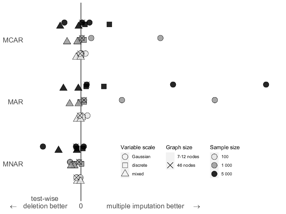
The following trends are apparent: For $n=100$, there were virtually no differences in the performance of test-wise deletion vs. multiple imputation, and the differences were most pronounced for $n=5\,000$. For Gaussian variables, multiple imputation outperformed test-wise deletion in almost all ‘MCAR’ and ‘MAR’ scenarios, but not in the ‘MNAR’ scenarios. For discrete variables, the same trend can be observed, but the advantage of multiple imputation only occurred for $n=5\,000$. For mixed variables, test-wise deletion outperformed multiple imputation in all simulation scenarios.

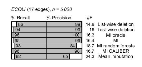
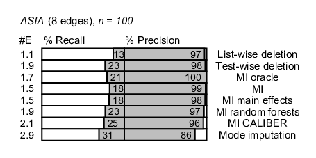
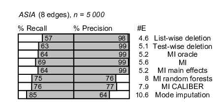
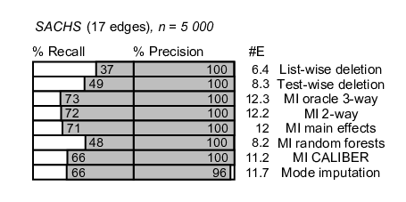
More detailed results are shown in Figures 8 and 9, and in the tables in the Online Supplement. The main observations are as follows: First, the edge recall was generally largest in the scenarios with Gaussian variables, smaller for discrete variables and very small for mixed variables. Further, while an average precision of more than 95 % was attained by a subset of the missing data methods in all Gaussian and discrete scenarios, this was not the case for the mixed scenarios. This is in line with earlier results using data without missing values (Andrews et al., 2018) and indicates that causal discovery using mixed data is a particularly challenging task.

As expected, list-wise deletion resulted in sparse graphs with large (structural) Hamming distances, due to the low power. An exception occurred in the MEHRA ‘MCAR’ scenarios with $n=100$ and $m=5\,000$, where list-wise deletion resulted in denser graphs than test-wise deletion. This seemingly paradoxical behaviour can be explained as follows. The PC-algorithm starts with marginal tests and proceeds to conditional testing only if the nodes still have enough neighbours to be included in the conditioning set. Under list-wise deletion, only few edges remain after the marginal phase, hence the number of conditional tests performed is small. Under test-wise deletion, more edges survive the marginal phase, hence more conditional tests are performed, but this leads to the deletion of most remaining edges due to the very low power of the CG-test conditioning on the categorical MEHRA variables with 6–31 categories.

Single imputation by the column mean or mode led to graphs that were ‘too large’ (many edges but low precision). In order to understand why this happened, consider the structure $X\rightarrow Y\rightarrow Z$, implying $X\mathchoice{\mathrel{\hbox to0.0pt{$\displaystyle\perp$\hss}\mkern 4.0mu{\displaystyle\perp}}}{\mathrel{\hbox to0.0pt{$\textstyle\perp$\hss}\mkern 4.0mu{\textstyle\perp}}}{\mathrel{\hbox to0.0pt{$\scriptstyle\perp$\hss}\mkern 4.0mu{\scriptstyle\perp}}}{\mathrel{\hbox to0.0pt{$\scriptscriptstyle\perp$\hss}\mkern 4.0mu{\scriptscriptstyle\perp}}}Z\mid Y$ but $X\not\mathchoice{\mathrel{\hbox to0.0pt{$\displaystyle\perp$\hss}\mkern 4.0mu{\displaystyle\perp}}}{\mathrel{\hbox to0.0pt{$\textstyle\perp$\hss}\mkern 4.0mu{\textstyle\perp}}}{\mathrel{\hbox to0.0pt{$\scriptstyle\perp$\hss}\mkern 4.0mu{\scriptstyle\perp}}}{\mathrel{\hbox to0.0pt{$\scriptscriptstyle\perp$\hss}\mkern 4.0mu{\scriptscriptstyle\perp}}}Z$. If $Y$ contains missing values and these are replaced by the column mean or mode, it is very likely that after conditioning on the imputed version of $Y$, there remains a residual association between $X$ and $Z$. However, the sample size is as large as if the data had been complete to begin with, and the fact that values were imputed is not taken into account by the testing procedure. Hence, the null hypothesis is rejected with a probability larger than the nominal test level, so that the resulting graph is more likely to contain an edge between $X$ and $Z$.

Test-wise deletion performed well overall. The results using the correction methods proposed by Tu et al., 2019 are not shown in Figures 8 and 9, as they were very similar to those using test-wise deletion without correction. This is not surprising, as the missingness mechanisms chosen for the simulation did not require these corrections. Tu et al., 2019 and Tu et al., 2020 showed that if they are required (which is usually not known in real data analyses), using the corrections improves the performance; we conclude that if they are not required, the performance is at least not substantially worsened.

Concerning multiple imputation, we observed that parametric imputation using interaction terms was computationally infeasible (producing errors) in many repetitions, especially for the datasets with mixed variables. See the Online Supplement for more information. We obtained inconclusive results for the usefulness of the two variants of random forest imputation. In the scenarios with only Gaussian or only categorical variables, the rf variant often produced graphs with a lower precision and worse Hamming distance than parametric imputation, and the CALIBER variant often ranged between parametric and rf imputation in terms of different evaluation metrics. In the scenarios with mixed variables, the performance of the two random forest methods was usually similar and also comparable to that of parametric imputation. The main difference between the two random forest options lies in how they guarantee that the multiply imputed values are sufficiently different from each other (in order to properly account for the uncertainty in the missing values). Using the rf option, a specified number of trees is fitted and one tree is chosen at random. A prediction is made using this tree and the imputed value is randomly drawn from among the observed values that are in the same leaf as the prediction. The CALIBERrfimpute functions fit the random forest model on a bootstrap sample of the observed data. The imputed value is then either the best prediction plus a normal error (continuous case) or the predicted value from just one of the trees (discrete case). Based on our simulation results, we conclude that the CALIBER version is more appropriate for conditional independence testing, and we conjecture that the difference between the two versions is less pronounced when the goal is e.g. estimation of a regression coefficient.

The ECOLI_large results in Figure 9 demonstrate the potential of the hybrid method. For $n=100$, test-wise deletion outperformed parametric multiple imputation (‘MI’ in the figure) in terms of the average precision and Hamming distance (34.9 for test-wise deletion vs. 35.8 for multiple imputation; see Online Supplement). Using the hybrid method A, the recall was as good as when using oracle multiple imputation, and the average Hamming distance was only 34.2. CALIBER random forest imputation also performed well and yielded an average Hamming distance of 34.8. We expect the differences to be larger in scenarios with even more variables.

References

- Ahrens et al., (2017) Ahrens, W., Siani, A., Adan, R., De Henauw, S., Eiben, G., Gwozdz, W., Hebestreit, A., Hunsberger, M., Kaprio, J., Krogh, V., Lissner, L., Mólnar, D., Moreno, L. A., Page, A., Pico, C., Reisch, L., Smith, R. M., Tornaritis, M., Veidebaum, T., Williams, G., Pohlabeln, H., and Pigeot, I. on behalf of the I.Family consortium (2017). Cohort profile: The transition from childhood to adolescence in European children – how I.Family extends the IDEFICS cohort. International Journal of Epidemiology, 46(5):1394–1395j.
- Alekseyenko et al., (2011) Alekseyenko, A. V., Lytkin, N. I., Ai, J., Ding, B., Padyukov, L., Aliferis, C. F., and Statnikov, A. (2011). Causal graph-based analysis of genome-wide association data in rheumatoid arthritis. Biology Direct, 6(1):25.
- Andrews et al., (2018) Andrews, B., Ramsey, J., and Cooper, G. F. (2018). Scoring Bayesian networks of mixed variables. International Journal of Data Science and Analytics, 6(1):3–18.
- Andrews et al., (2021) Andrews, R., Foraita, R., Didelez, V., and Witte, J. (2021). A practical guide to causal discovery with cohort data. Working paper.
- Bartlett et al., (2015) Bartlett, J. W., Seaman, S. R., White, I. R., Carpenter, J. R., and the Alzheimer’s Disease Neuroimaging Initiative (2015). Multiple imputation of covariates by fully conditional specification: Accommodating the substantive model. Statistical Methods in Medical Research, 24(4):462–487.
- Bessler and Yang, (2003) Bessler, D. A. and Yang, J. (2003). The structure of interdependence in international stock markets. Journal of International Money and Finance, 22(2):261–287.
- Börnhorst et al., (2016) Börnhorst, C., Siani, A., Russo, P., Kourides, Y., Sion, I., Molnár, D., Moreno, L. A., Rodríguez, G., Ben-Shlomo, Y., Howe, L., Lissner, L., Mehlig, K., Regber, S., Bammann, K., Foraita, R., Ahrens, W., and Tilling, K. (2016). Early life factors and inter-country heterogeneity in BMI growth trajectories of European children: The IDEFICS study. PLOS ONE, 11(2):1–20.
- Carpenter and Kenward, (2013) Carpenter, J. R. and Kenward, M. G. (2013). Multiple Imputation and Its Application. John Wiley & Sons, Chichester, UK.
- Colombo and Maathuis, (2014) Colombo, D. and Maathuis, M. H. (2014). Order-independent constraint-based causal structure learning. The Journal of Machine Learning Research, 15(1):3741–3782.
- Cunningham, (2021) Cunningham, S. (2021). Causal Inference: The Mixtape. Yale University Press, New Haven, Connecticut, USA.
- Daniel et al., (2012) Daniel, R. M., Kenward, M. G., Cousens, S. N., and De Stavola, B. L. (2012). Using causal diagrams to guide analysis in missing data problems. Statistical Methods in Medical Research, 21(3):243–256.
- Didelez, (2018) Didelez, V. (2018). Causal concepts and graphical models. In Maathuis, M., Drton, M., Lauritzen, S., and Wainwright, M., editors, Handbook of Graphical Models, chapter 15, pages 355–382. CRC Press.
- Didelez et al., (2010) Didelez, V., Kreiner, S., and Keiding, N. (2010). Graphical models for inference under outcome-dependent sampling. Statistical Science, 25(3):368–387.
- Doove et al., (2014) Doove, L. L., Van Buuren, S., and Dusseldorp, E. (2014). Recursive partitioning for missing data imputation in the presence of interaction effects. Computational Statistics & Data Analysis, 72:92–104.
- Doretti et al., (2018) Doretti, M., Geneletti, S., and Stanghellini, E. (2018). Missing data: a unified taxonomy guided by conditional independence. International Statistical Review, 86(2):189–204.
- Ebert-Uphoff and Deng, (2012) Ebert-Uphoff, I. and Deng, Y. (2012). Causal discovery for climate research using graphical models. Journal of Climate, 25(17):5648–5665.
- Enders, (2010) Enders, C. K. (2010). Applied Missing Data Analysis. The Guilford Press, New York, USA.
- Fisher, (1924) Fisher, R. A. (1924). The distribution of the partial correlation coefficient. Metron, 3:329–332.
- Foraita et al., (2020) Foraita, R., Friemel, J., Günther, K., Behrens, T., Bullerdiek, J., Nimzyk, R., Ahrens, W., and Didelez, V. (2020). Causal discovery of gene regulation with incomplete data. Journal of the Royal Statistical Society: Series A (Statistics in Society), 183(4):1747–1775.
- Foraita et al., (2021) Foraita, R., Witte, J., Börnhorst, C., De Henauw, S., Gwozdz, W., Krogh, V., Lissner, L., Lauria, F., Molnár, D., Moreno, L., Page, A., Reisch, L., Veidebaum, T., Tornaritis, M., Pigeot, I., and Didelez, V. (2021). A longitudinal causal graph analysis investigating modifiable risk factors and obesity in a European cohort of children and adolescents. Working paper.
- Friedman, (1997) Friedman, N. (1997). Learning belief networks in the presence of missing values and hidden variables. In Fisher, D. H., editor, Proceedings of the Fourteenth International Conference on Machine Learning (ICML ’97), pages 125–133. Morgan Kaufmann Publishers.
- Gain and Shpitser, (2018) Gain, A. and Shpitser, I. (2018). Structure learning under missing data. Proceedings of Machine Learning Research, 72:121–132.
- Greenland et al., (1999) Greenland, S., Pearl, J., and Robins, J. M. (1999). Causal diagrams for epidemiologic research. Epidemiology, 10(1):37–48.
- Hardt et al., (2012) Hardt, J., Herke, M., and Leonhart, R. (2012). Auxiliary variables in multiple imputation in regression with missing X: a warning against including too many in small sample research. BMC Medical Research Methodology, 12(1):184.
- Hebestreit et al., (2016) Hebestreit, A., Barba, G., De Henauw, S., Eiben, G., Hadjigeorgiou, C., Kovács, É., Krogh, V., Moreno, L. A., Pala, V., Veidebaum, T., Wolters, M., and Börnhorst, C. on behalf of the IDEFICS Consortium (2016). Cross-sectional and longitudinal associations between energy intake and BMI z-score in European children. International Journal of Behavioral Nutrition and Physical Activity, 13(1):1–11.
- Hughes et al., (2019) Hughes, R. A., Heron, J., Sterne, J. A., and Tilling, K. (2019). Accounting for missing data in statistical analyses: multiple imputation is not always the answer. International Journal of Epidemiology, 48(4):1294–1304.
- Hughes et al., (2014) Hughes, R. A., White, I. R., Seaman, S. R., Carpenter, J. R., Tilling, K., and Sterne, J. A. (2014). Joint modelling rationale for chained equations. BMC Medical Research Methodology, 14(1):1–10.
- Kalisch et al., (2012) Kalisch, M., Mächler, M., Colombo, D., Maathuis, M. H., and Bühlmann, P. (2012). Causal inference using graphical models with the R package pcalg. Journal of Statistical Software, 47(11):1–26.
- Lauritzen, (1990) Lauritzen, S. L. (1990). Graphical Models. Oxford University Press, Oxford, UK.
- Lauritzen and Wermuth, (1989) Lauritzen, S. L. and Wermuth, N. (1989). Graphical models for associations between variables, some of which are qualitative and some quantitative. The Annals of Statistics, 17(1):31–57.
- Lee et al., (2017) Lee, B. Y., Bartsch, S. M., Mui, Y., Haidari, L. A., Spiker, M. L., and Gittelsohn, J. (2017). A systems approach to obesity. Nutrition Reviews, 75(suppl_1):94–106.
- Little and Rubin, (2002) Little, R. J. A. and Rubin, D. B. (2002). Statistical Analysis with Missing Data. Wiley & Sons, Hoboken, New Jersey, USA, 2nd edition.
- Maathuis et al., (2009) Maathuis, M. H., Kalisch, M., and Bühlmann, P. (2009). Estimating high-dimensional intervention effects from observational data. The Annals of Statistics, 37(6A):3133–3164.
- Mealli and Rubin, (2015) Mealli, F. and Rubin, D. B. (2015). Clarifying missing at random and related definitions, and implications when coupled with exchangeability. Biometrika, 102(4):995–1000.
- Meek, (1995) Meek, C. (1995). Causal inference and causal explanation with background knowledge. In Besnard, P. and Hanks, S., editors, Proceedings of the Eleventh Conference on Uncertainty in Artificial Intelligence (UAI-95), pages 403–410. Morgan Kaufmann Publishers.
- Meng, (1994) Meng, X.-L. (1994). Multiple-imputation inferences with uncongenial sources of input. Statistical Science, 9(4):538–558.
- Meng and Rubin, (1992) Meng, X.-L. and Rubin, D. B. (1992). Performing likelihood ratio tests with multiply-imputed data sets. Biometrika, 79(1):103–111.
- Moffa et al., (2017) Moffa, G., Catone, G., Kuipers, J., Kuipers, E., Freeman, D., Marwaha, S., Lennox, B. R., Broome, M. R., and Bebbington, P. (2017). Using directed acyclic graphs in epidemiological research in psychosis: an analysis of the role of bullying in psychosis. Schizophrenia Bulletin, 43(6):1273–1279.
- Mohan and Pearl, (2021) Mohan, K. and Pearl, J. (2021). Graphical models for processing missing data. Journal of the American Statistical Association, 116(534):1023–1037.
- Mohan et al., (2013) Mohan, K., Pearl, J., and Tian, J. (2013). Graphical models for inference with missing data. In Burges, C. J. C., Bottou, M. W., Ghahramani, Z., and Weinberger, K. Q., editors, Advances in Neural Information Processing Systems 26 (NIPS-2013), pages 1277–1285.
- Moreno-Betancur et al., (2018) Moreno-Betancur, M., Lee, K. J., Leacy, F. P., White, I. R., Simpson, J. A., and Carlin, J. B. (2018). Canonical causal diagrams to guide the treatment of missing data in epidemiologic studies. American Journal of Epidemiology, 187(12):2705–2715.
- Morgan and Winship, (2014) Morgan, S. L. and Winship, C. (2014). Counterfactuals and Causal Inference. Cambridge University Press, Cambridge, UK, 2nd edition.
- Morris et al., (2014) Morris, T. P., White, I. R., and Royston, P. (2014). Tuning multiple imputation by predictive mean matching and local residual draws. BMC Medical Research Methodology, 14(1):1–13.
- Noghrehchi et al., (2021) Noghrehchi, F., Stoklosa, J., Penev, S., and Warton, D. I. (2021). Selecting the model for multiple imputation of missing data: Just use an IC! Statistics in Medicine, 40(10):2467–2497.
- Pearl, (1988) Pearl, J. (1988). Probabilistic Reasoning in Intelligent Systems: Networks of Plausible Inference. Morgan Kaufmann Publishers, San Francisco, California.
- Pigeot et al., (2015) Pigeot, I., Sobotka, F., Kreiner, S., and Foraita, R. (2015). The uncertainty of a selected graphical model. Journal of Applied Statistics, 42(11):2335–2352.
- Pohlabeln et al., (2017) Pohlabeln, H., Rach, S., De Henauw, S., Eiben, G., Gwozdz, W., Hadjigeorgiou, C., Molnár, D., Moreno, L. A., Russo, P., Veidebaum, T., and Iris Pigeot on behalf of the IDEFICS consortium (2017). Further evidence for the role of pregnancy-induced hypertension and other early life influences in the development of ADHD: results from the IDEFICS study. European Child & Adolescent Psychiatry, 26(8):957–967.
- Rau and Scheines, (2012) Rau, M. A. and Scheines, R. (2012). Searching for variables and models to investigate mediators of learning from multiple representations. In Yacef, K., Zaïane, O., Hershkovitz, A., Yudelson, M., and Stamper, J., editors, Proceedings of the 5th International Conference on Educational Data Mining, pages 110–117.
- Ray et al., (2015) Ray, S., Haney, M., Hanson, C., Biswal, B., and Hanson, S. J. (2015). Modeling causal relationship between brain regions within the drug-cue processing network in chronic cocaine smokers. Neuropsychopharmacology, 40(13):2960–2968.
- Roberts and Winters, (2013) Roberts, S. and Winters, J. (2013). Linguistic diversity and traffic accidents: Lessons from statistical studies of cultural traits. PLOS ONE, 8(8):e70902.
- Rubin, (1976) Rubin, D. B. (1976). Inference and missing data. Biometrika, 63(3):581–592.
- Rubin, (1987) Rubin, D. B. (1987). Multiple Imputation for Nonresponse in Surveys. John Wiley & Sons, New York, USA.
- Schafer, (1997) Schafer, J. L. (1997). Analysis of Incomplete Multivariate Data. CRC, Boca Raton, Florida, USA.
- Scutari, (2020) Scutari, M. (2020). Bayesian network models for incomplete and dynamic data. Statistica Neerlandica, 74(3):397–419.
- Seaman et al., (2013) Seaman, S., Galati, J., Jackson, D., and Carlin, J. (2013). What is meant by ‘missing at random’? Statistical Science, 28(2):257–268.
- Shah et al., (2014) Shah, A. D., Bartlett, J. W., Carpenter, J., Nicholas, O., and Hemingway, H. (2014). Comparison of random forest and parametric imputation models for imputing missing data using MICE: a CALIBER study. American Journal of Epidemiology, 179(6):764–774.
- Sokolova et al., (2017) Sokolova, E., von Rhein, D., Naaijen, J., Groot, P., Claassen, T., Buitelaar, J., and Heskes, T. (2017). Handling hybrid and missing data in constraint-based causal discovery to study the etiology of ADHD. International Journal of Data Science and Analytics, 3(2):105–119.
- Spirtes et al., (2000) Spirtes, P., Glymour, C. N., and Scheines, R. (2000). Causation, Prediction, and Search. MIT press, Cambridge, Massachusetts, 2nd edition.
- Steck and Jaakkola, (2003) Steck, H. and Jaakkola, T. (2003). Bias-corrected bootstrap and model uncertainty. In Thrun, S., Saul, L., and Schölkopf, B., editors, Advances in Neural Information Processing Systems 16 (NIPS 2003), pages 521–528.
- Strobl et al., (2018) Strobl, E. V., Visweswaran, S., and Spirtes, P. L. (2018). Fast causal inference with non-random missingness by test-wise deletion. International Journal of Data Science and Analytics, 6(1):47–62.
- Tennant et al., (2021) Tennant, P. W. G., Murray, E. J., Arnold, K. F., Berrie, L., Fox, M. P., Gadd, S. C., Harrison, W. J., Keeble, C., Ranker, L. R., Textor, J., Tomova, G. D., Gilthorpe, M. S., and Ellison, G. T. H. (2021). Use of directed acyclic graphs (DAGs) to identify confounders in applied health research: review and recommendations. International Journal of Epidemiology, 50(2):620–632.
- Tsamardinos et al., (2006) Tsamardinos, I., Brown, L. E., and Aliferis, C. F. (2006). The max-min hill-climbing Bayesian network structure learning algorithm. Machine Learning, 65(1):31–78.
- Tu et al., (2019) Tu, R., Zhang, C., Ackermann, P., Mohan, K., Kjellström, H., and Zhang, K. (2019). Causal discovery in the presence of missing data. In Chaudhuri, K. and Sugiyama, M., editors, Proceedings of the 22nd International Conference on Artificial Intelligence and Statistics (AISTATS 2019), pages 1762–1770. PMLR.
- Tu et al., (2020) Tu, R., Zhang, K., Ackermann, P., Bertilson, B. C., Glymour, C., Kjellström, H., and Zhang, C. (2020). Causal discovery in the presence of missing data. arXiv preprint arXiv:1807.04010.
- van Buuren, (2018) van Buuren, S. (2018). Flexible Imputation of Missing Data. CRC, Boca Raton, Florida, USA.
- van Buuren and Groothuis-Oudshoorn, (2011) van Buuren, S. and Groothuis-Oudshoorn, K. (2011). mice: Multivariate imputation by chained equations in R. Journal of Statistical Software, 45(3):1–67.
- Vandenbroeck et al., (2017) Vandenbroeck, P., Goossens, J., and Clemens, M. (2017). Foresight, tackling obesities: future choices building the obesity system map. Report by the UK Government Office for Science. www.gov.uk/government/publications/reducing-obesity-obesity-system-map.
- Westreich, (2012) Westreich, D. (2012). Berkson’s bias, selection bias, and missing data. Epidemiology, 23(1):159–164.
- Zhang, (2008) Zhang, J. (2008). On the completeness of orientation rules for causal discovery in the presence of latent confounders and selection bias. Artificial Intelligence, 172(16–17):1873–1896.