Robust Privacy-Preserving Motion Detection and Object Tracking in Encrypted Streaming Video
Abstract
Video privacy leakage is becoming an increasingly severe public problem, especially in cloud-based video surveillance systems. It leads to the new need for secure cloud-based video applications, where the video is encrypted for privacy protection. Despite some methods that have been proposed for encrypted video moving object detection and tracking, none has robust performance against complex and dynamic scenes. In this paper, we propose an efficient and robust privacy-preserving motion detection and multiple object tracking scheme for encrypted surveillance video bitstreams. By analyzing the properties of the video codec and format-compliant encryption schemes, we propose a new compressed-domain feature to capture motion information in complex surveillance scenarios. Based on this feature, we design an adaptive clustering algorithm for moving object segmentation with an accuracy of 44 pixels. We then propose a multiple object tracking scheme that uses Kalman filter estimation and adaptive measurement refinement. The proposed scheme does not require video decryption or full decompression and has a very low computation load. The experimental results demonstrate that our scheme achieves the best detection and tracking performance compared with existing works in the encrypted and compressed domain. Our scheme can be effectively used in complex surveillance scenarios with different challenges, such as camera movement/jitter, dynamic background, and shadows.
Keywords Encrypted video processing cloud computing video surveillance motion detection object tracking compressed-domain feature
1 Introduction
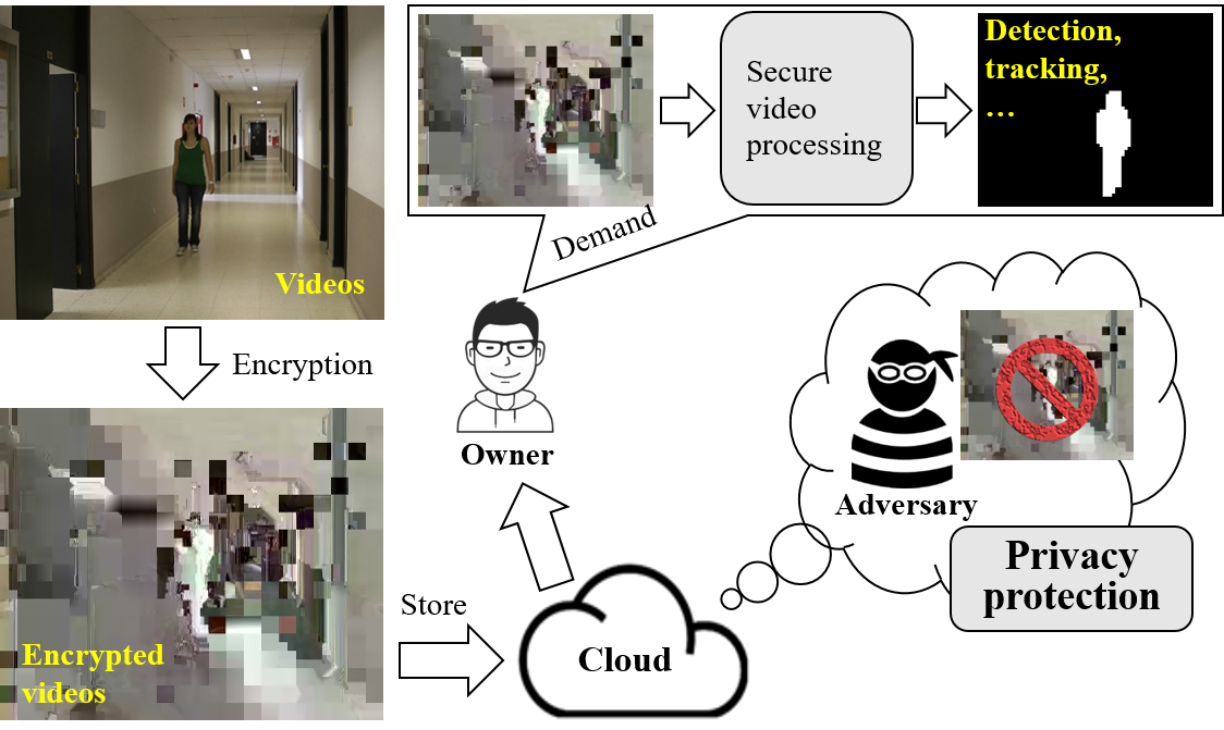
Surveillance cameras play a significant role in public security. The resulting surveillance videos are usually compressed into bitstreams for efficient transmission and storage. Due to the heavy burden of storing and processing massive video data, the video owner will prefer to outsource the expensive data storage and video signal processing tasks to the cloud, so as to enjoy conveniently personalized computing services and easy remote access from phones or PCs. However, storing unencrypted data in the cloud can threaten the privacy of the people that have been recorded. The consequences can range from family privacy infringement to the leakage of secret information. To avoid the exposure of video content, we must encrypt video bitstreams before storing them in the cloud server. However, the encryption of video bitstream data poses a dilemma for the cloud, making subsequent video processing more complicated and difficult. Therefore, it is urgently necessary to develop a secure cloud-based solution that can directly analyze and process an encrypted video stream in real time, so that applications such as anomaly alarms, abnormal object detection, and visual tracking can operate as usual in intelligent monitoring systems. We illustrate this critical problem in Fig. 1.
Signal processing in the encrypted domain (SPED) (Lagendijk et al. 2013), which enables the processing of ciphertext data without decryption, is a promising solution for privacy-preserving cloud computing. Numerous SPED-based cloud computing applications have recently been proposed by using homomorphic encryption (HE) (Paillier 1999; Brakerski et al. 2014).
To reduce ciphertext expansion, an image homomorphic encryption scheme (Zheng and Huang 2013) is proposed. In (Erkin et al. 2009), Erkin et al. presented a privacy-enhanced face recognition system based on the Paillier encryption. Troncoso-Pastoriza et al. (Troncoso-Pastoriza et al. 2013) proposed a private face verification system by employing quasi-fully HE. Hu et al. (Hu et al. 2016) proposed an outsourced feature extraction protocol on encrypted images using somewhat HE. In (Hu et al. 2016), Hu et al. presented a secure nonlocal denoising algorithm on encrypted images with the Paillier encryption. Some reversible data hiding schemes (Xiang and Luo 2018; Zhang et al. 2016; Zheng et al. 2019) are proposed on encrypted images using HE. However, this HE-based approach is inefficient and impractical for real-time video encryption due to the formidable size of the computations and the huge storage requirements. For real-time encrypted video surveillance, one essential requirement is to utilize an efficient video bitstream encryption scheme to ensure that the required processing can be directly performed on the encrypted bitstream. In the following, we will mainly focus on the format-compliant video encryption, which encrypts only certain specific syntax elements in the bitstream, thus preserving the original video format and allowing the encrypted bitstream to be correctly parsed by common video decoders.
Motion detection and tracking are the key components of intelligent surveillance systems; these processes involve locating the positions of moving objects and tracking them over time in every frame of a surveillance video. Existing video motion detection and tracking schemes in the plaintext domain can be classified into two categories based on the methods used: the first is performed in the pixel domain, and extracts features from visual data using techniques such as optical flow (Duncan and Chou 1992), background modeling/subtraction (Stauffer and Grimson 1999; Maddalena and Petrosino 2012; St-Charles et al. 2015), and convolutional neural networks (Ren et al. 2017; Redmon et al. 2016), while the second operates in the compressed domain, and relies on syntax elements extracted from the video bitstream, such as macroblock coding bits, macroblock partition, motion vectors, quantization parameters and discrete cosine transform (DCT) coefficients (Khatoonabadi and Bajic 2013; Dey and Kundu 2013; Zhao et al. 2018). The first type of approach is computationally expensive and often has bottlenecks in real-time operations due to the high complexity of these algorithms and the enormous amounts of data involved in processing. Moreover, without fully video decompression, pixel-domain approaches cannot be directly performed on cloud surveillance video data stored in compressed form. In contrast, compressed-domain approaches can run at high speeds, since they require only partial decoding of the bitstream. Therefore, compressed-domain approaches are preferable for secure real-time video surveillance in cloud computing.
There are already some privacy-preserving video surveillance schemes relying on pixel-domain motion detection techniques, where the encryption methods are applied to the decompressed video frames. Upmanyu et al. (Upmanyu et al. 2009) designed a privacy-preserving motion detection and tracking system for encrypted surveillance video by using a secret sharing scheme with the Chinese remainder theorem. In (Zeng et al. 2010), Zeng et al. proposed a secure object detection scheme based on Paillier encryption. Chu et al. (Chu et al. 2013) presented a privacy-preserving moving object detection scheme that scrambles each frame with matrix permutation and multiplication. In (Jin et al. 2016), Jin et al. proposed a video foreground extraction method based on chaotic-mapping video encryption. In (Lin et al. 2017), Lin et al. proposed a system that separated video pixels into two parts, one of which was kept unchanged and the other encrypted with pixel scrambling. Since the resultant encrypted video are encrypted frame sequences in (Chu et al. 2013; Jin et al. 2016; Lin et al. 2017), the adaptive Gaussian mixture models (GMM) (Stauffer and Grimson 1999) can be applied to obtain the motion detection results. However, frame-encryption based schemes usually result in high execution times and also have apparent drawbacks in terms of transmission and storage because they do not support video compression.
Following video compression standards and format-compliant video encryption techniques (Stutz and Uhl 2012), some recent works enable motion detection and tracking on encrypted video bitstreams. Guo et al. (Guo et al. 2017) designed a motion detection and tracking scheme for an H.264/AVC (Wiegand et al. 2003) bitstream encrypted with the format-compliant encryption proposed in (Xu et al. 2014). They proposed a feature based on the length of motion vector difference (LMVD), and a region update algorithm for object tracking. In (Ma et al. 2018), Ma et al. used the format-compliant encryption scheme proposed in (Shahid and Puech 2014) to encrypt an H.265/HEVC (Sullivan et al. 2012) video, and then shuffle the coding tree units (CTU). To perform motion detection and tracking on encrypted H.265 bitstreams, they proposed to extract features from coding bits (CB) and partition depth (PD). These bitstream-based schemes have the advantages of low storage requirements and high computational efficiency. However, these schemes can only detect objects in 1616 block level or CTU level (between 1616 pixels and 6464 pixels). Moreover, they do not have robust detection and tracking performance in complex surveillance scenarios presenting different challenges, such as camera shaking/moving, shadow, dynamic background, etc.
In this paper, we focus on secure motion detection and tracking in the cloud-based video surveillance system, where surveillance video is compressed and encrypted with format-compliant video encryption. Without loss of generality, we use H.264/AVC as an example to illustrate our scheme, considering its popularity in video surveillance compression system. We propose a privacy-preserving motion detection and tracking scheme to be applied to encrypted video bitstream in the cloud. More specifically, we propose a novel compressed-domain feature known as the density of non-zero residual coefficient (DNRC) to extract motion information from the encrypted video bitstream. The proposed feature enables us to successfully locate smaller objects than the existing features used in (Guo et al. 2017; Ma et al. 2018). To efficiently separate motion regions from the background, we design an adaptive and non-parameterized clustering method based on the density-based spatial clustering of applications with noise (DBSCAN) (Ester et al. 1996). We then propose a reliable object tracking scheme with Kalman filter estimation and an adaptive bounding box refinement method against different challenges in real surveillance tasks. The major contributions in this paper can be summarized as follows.
- •
We propose a novel feature, DNRC, extracted from encrypted video bitstreams. The proposed feature locates objects with an accuracy of 44 pixels, which is more precise than the 1616 block-level of previous works in the encrypted and compressed domain.
- •
We design an adaptive and non-parameterized clustering algorithm based on DBSCAN, which can effectively segment moving objects from the dynamic background.
- •
We propose a reliable multi-object tracking scheme based on Kalman filtering by adaptively refining the observation data. Our method has robust performance in complex scenarios presenting different challenges, such as occlusion, camera moving/jittering, shadow.
- •
Our secure motion detection and tracking scheme allows for effective detection, robust tracking, and fast computation. The experimental results show that the proposed algorithms achieve the best performance among comparable schemes for encrypted bitstream video.
The rest of this paper is organized as follows. Section 2 presents our threat model and encryption scheme. In Section 3, we introduce the feature DNRC, the proposed clustering algorithm, and our motion tracking scheme. The experimental results conducted on different surveillance video databases are presented in Section 4, and some discussions are provided in Section 5. Finally, we draw conclusions in Section 6.
2 Problem Statement
2.1 Threat Model

In this paper, we consider a non-interactive video motion detection and tracking system that involves only two parties: the video data owner and the cloud server. The owner uses several devices simultaneously, such as surveillance cameras, computers, smartphones, tablets, etc. A sketch of our system model is shown in Fig. 2. We assume that the owner’s storage and computation resources are limited, and that in order to deal with a vast volume of video data, the owner needs to outsource data storage and computing tasks to the cloud.
Following most existing privacy-preserving multimedia outsourcing schemes (Hsu et al. 2012; Hu et al. 2016), we adopt a semi-honest setting throughout this paper. Specifically, the cloud server is considered a semi-trusted adversary in our application scenario, which honestly executes the proposed protocol but attempts to learn additional sensitive video content, such as human faces and card security codes, from the encrypted video and all the exchanged messages. To avoid the leakage of private or sensitive content to the cloud, the owner prefers to store encrypted video on the cloud storage server. In this paper, we use format-compliant selective encryption, a widespread technique in multimedia encryption, due to its advantages in maintaining a balance between privacy and convenience. More detailed discussions of privacy protection with selective video encryption can be found in (Shahid et al. 2011). By using our protocols, the cloud server can detect moving objects and obtain object trajectories. However, without the decryption keys, the cloud server cannot deduce sensitive and private information about the individuals in the video.
2.2 Video Encryption Scheme
In our video encryption scheme, we encrypt the codewords of three syntax elements, i.e., motion vector difference (MVD), residual data, and intra-prediction mode (IPM). Each syntax element is encrypted according to its specified coding method.
2.2.1 MVD Encryption
MVDs are encoded with the -order Exp-Golomb (EG) code in H.264/AVC. For example, the codeword structure of EG0 ( = 0) can be represented as
where “ zeros” indicates the length of “suffix”, and “suffix” contains -bits of the encoded information. We encrypt the last bit of the non-zero MVD codeword. The last bit encryption may change the sign of MVD and satisfies the format compliance without bit increase.
2.2.2 Residual Data Encryption
The residual data are obtained from the intra or inter predictions. After transformation and quan-tization, the data are entropy encoded using CAVLC in the baseline profile. Using CAVLC, each codeword of the residual data can be represented as
The codeword of level can be further represented as
We encrypt all bits in the codeword of sign_of_traillingones and the last bits in the codeword of level. For format compliance, level cannot be encrypted when its suffix length is equal to 0.
2.2.3 IPM Encryption
In the high profile of H.264, three types of intra coding are supported to be encrypted, which are denoted as Intra_44, Intra_88, and Intra_1616. The IPM for Intra_1616 blocks are specified in the mb_type (macroblock type), which defines other block parameters like coded block pattern (CBP). The mb_type is encoded with the Exp-Golomb code. To ensure format compliance of the encrypted bitstream, we cannot change the CBPs of mb_type when encrypting IPM. According to the mb_type table for the I frame (Telecom, ITU 2003), only the last bit of the codewords of all mb_type of Intra_1616 can be encrypted in the I frame. However, this encryption method cannot be applied to those Intra_1616 blocks in the P frame due to the different mb_type tables used in the I and P frames (Telecom, ITU 2003). To keep the length of the codeword unchanged and format-compliant, we only encrypted the last bit of those codewords of mb_types in the set of
The Intra_44 and Intra_88 blocks use the same method to code their IPMs. The H.264 codec provides every 44/88 block with a most probable intra prediction model (MP-IPM) based on the neighbor blocks. If the MP-IPM is equal to the lowest-bit-cost intra prediction model, then the codeword of IPM only consists of one flag bit “1”. Otherwise, the codeword is composed of one flag bit “0” and three bits fixed-length code indicating one of the other eight modes except MP-IPM. These three bits can be encrypted without format conflict concern. Generally, our encryption scheme encrypts all IPMs in the Intra_44 block and Intra_88 for the I and P frames. The target bits for encryption are first extracted from the video bitstream and then encrypted by a standard cipher, such as RC6 block cipher. The enciphered bits are placed back into the bitstream to replace the original bits. During video decryption, the enciphered bits in the encrypted video bitstream are decrypted to the plaintext bits. We use these plaintext bits to replace the corresponding enciphered bits in the video bitstream. Note that the proposed technique for object tracking is not designed to rely on this specific video encryption scheme. We will discuss the extension to other video coding standards and video bitstream encryption schemes in Section 5.4.

3 Proposed Privacy-Preserving Motion Detection and Tracking Scheme
We summarize our scheme’s steps in Fig. 3, which includes feature extraction, clustering for initial motion detection, and object tracking and refinement. We extract the proposed feature in the encrypted bitstream without fully video decoding and design a temporal filter for smoothing (Section III-A). The motion detection and tracking procedure is implemented frame by frame. Based on the extracted features, we propose a clustering algorithm to perform segmentation and obtain initial detection results (Section III-B). We then propose a refinement strategy and adopt adaptive Kalman filtering to obtain precise detection results and track moving objects (Section III-C).
3.1 Feature Extraction
In the video encoding process, the macroblocks in a motion region always contain considerable variation in pixel values and many detail textures, When performing DCT on these macroblocks, a large number of residual coefficients are generated. There are two kinds of methods modifying the residual coefficients in existing format-compliant H.264 video encryption schemes, i.e., sign inversion and value modification on residual coefficients. Both the sign inversion and value modification do not change the number of non-zero residual coefficients in a luma block. Therefore, although the codewords of residual coefficients are encrypted in format-compliant video encryption schemes, the number of non-zero residual coefficients in every frame is preserved after video encryption. Some reports (Dey and Kundu 2013; Poppe et al. 2009; Sabirin and Kim 2012) have shown that the residuals are capable of detecting moving objects in the plaintext domain. Non-zero residual coefficients are more likely to be concentrated in the motion region, meaning that a block with more non-zero residual coefficients has a higher probability of being in the moving object region.
We divide the -th frame into non-overlapping 44 blocks . We can also use the sequence to represent the 2D matrix in a raster scan order. Without causing confusion, we sometimes use and in the following. According to the H.264/AVC compression standard, such a block is either located in a whole 44 transform block or combined with three more blocks to form an 88 transform block. Based on the above analysis, we propose a new feature, i.e., DNRC, in each 44 block . The proposed feature approximately assesses the density of non-zero residual coefficients within a 44 block. We use to count the number of non-zero residual coefficients in a 44 or 88 residual coefficient block.
We firstly consider the DNRC feature extraction in P frames. When using Intra_1616 prediction mode, the DC coefficients of each 44 block in the Intra_1616 macroblock are separated from the residual coefficient block to form another block, on which a Hadamard transform is performed. The total number of non-zero residual coefficients for then should increase by one if has a non-zero DC component. Hence, we compute the influence of the DC component on the DNRC of as
| (1) |
The DNRC of a 44 block is then defined as
| (2) |

When the H.264/AVC encoder additionally uses a transform block size of 88, it will produce an 88 residual coefficient block covering four 44 s, rather than four residual coefficient blocks size of 44. In order to extract feature information from such a in this case, we set the DNRC of as the number of non-zero residual coefficients in the 88 residual coefficient block. Considering that there are only 16(=44) elements in , we constrain its maximum DNRC to be 16. Thus, for a 44 block located in an 88 transform block , its DNRC value is computed as
| (3) |
where denotes the minimum operator. We illustrate some examples of DNRC extraction in 44 and 88 transform blocks in Fig. 4.
Since the H.264/AVC coder generates the prediction residual in the I frame by referring to the neighboring macroblock in the spatial domain, the residual data in the I frame cannot represent the motion information in the temporal domain. Thus, we compute the DNRC value in the I frame from the DNRC values in the neighboring P frames using the inverse distance weighted interpolation method (Tugrul and Polat 2014). Suppose that is the DNRC of the block in the -th frame. We initialize s in the I- frames as zeros, and then update in the I-frame as
| (4) |
where denotes the window size of the interpolation.
Although our DNRC feature can reflect the motion information, other pixel changes in the video content, including the foreground and background pixel changes, will also influence the DNRC feature. These DNRC values will create false-positive motion regions. For the DNRC values indicating real moving objects, we consider these false-positive values as “noises” in the feature sequence . These noise values are likely to be caused by dynamic background noise or compression quantizing noise, such as valley noise (a zero DNRC surrounded by consecutive non-zero DNRCs in the form of a valley) or spike noise (a short-term, non-zero DNRC sequence that appears abruptly in a zero sequence). For valley noise in the -th frame, we use the smallest DNRC in the (-1)-th and (+1)-th frames to replace the zero DNRC in the valley noise, while spike noise can be diminished by applying a lowpass filter along the temporal direction. Due to the sensitivity of DNRC between zero and non-zero, we also want to set zero the noisy DNRC values that need to be filtered out, and keep the normal DNRC values unchanged. Assume that the distribution of noise spikes is sparse, i.e., there is one noise spike approximately every frames. We use to denote a sub-set of frame indexes, i.e.,
| (5) |
The filtered DNRC value can then be obtained as
where is a function deciding whether the input is zero or not, i.e., . We denote all the filtered DNRC values in the -th frame by the sequence . As shown in Fig. 4, we can reshape into a 2D matrix , called the feature image, according to the positions of in . An example of the feature image can be seen in Fig. 5(c). Without causing confusion, we will use and in the following.
3.2 Clustering
Based on the feature image , we propose a clustering method to segment initial motion regions from the background. A large value of will make a great contribution to gathering other non-zero elements in into a cluster. In general, noise regions such as the shadows of moving objects usually have small DNRC values, and disperse into several small areas that are difficult to form into a complete cluster. In view of these characteristics, we propose an efficient and adaptive clustering algorithm based on DBSCAN, in which the number of clusters in a feature image need not be specified.
Let us denote the feature image consisting of all non-zero elements in by . Given a point and a radius , we define the -neighborhood as
| (8) |
where is a pre-defined distance between and .
If the point number of is greater than a threshold minPts, DBSCAN will consider a core point of a new cluster. Traditionally, minPts is usually set to one more than the cluster’s dimension, e.g., minPts = 3 in our application scenario. All the points in will form a temporary cluster of . If a point in this temporary cluster is a core point, all the points in will be included to form a new temporary cluster. This process is repeated until no more new points are added to the temporary cluster, and the final cluster of is obtained. After that, all the clusters are generated. The points that do not belong to any cluster are regarded as noise points.


The definition of the -neighborhood plays a central role in the clustering algorithm. To adapt to our application scenario, a point with a significant value should have a large radius . We must ensure that , since is the minimum Euclidean radius of an 8-adjacent connection. Thus, we set the radius of in our method as
| (9) |
where is a factor representing the clustering ability of DNRC that needs to be defined in the following.
We use to represent the mean of all s in . A higher value of indicates that the number of non-zero residual coefficients generally is larger on every pixel block. It mainly results from fast-moving objects in the frame or suddenly shaking background caused by camera movement/jitter. For a fast-moving object, clustering different parts into different small clusters with a small radius, respectively, can avoid involving too many false-positive regions. As for camera movement/jitter, small clusters can separate the suddenly changed background from real motion regions. Therefore, when the value of is higher, using a smaller radius can improve the detection accuracy and decrease the false positive rate. Conversely, a smaller indicates that the objects are moving slowly and the background is stable. We can use a large radius to generate large-size clusters to avoid missing the false-negatives points without worrying about covering the background regions. Thus, it is reasonable that is in inverse proportion to .
Specifically, we define as
| (10) |
where denotes the maximum operator. We use to evaluate the influence of the point on the core point , i.e.,
| (11) |
Consequently, we define the -neighborhood of in the proposed method as
| (12) |
where denotes the Euclidean distance between and . By combining the inequality with Eq. (9) and Eq. (11), we get
| (13) |
We denote the terms on the left-hand of the above inequality by , and rewrite Eq. (12) as
| (14) |
By comparing Eq. (8) and Eq. (14), we can see that we set and use to adapt the DBSCAN algorithm to our application scenario. Unlike the typical DBSCAN algorithm, we do not need to preset the radius . Thus, our clustering algorithm is adaptive and non-parameterized. We show an example of the clustering results in Fig.5(d).
The proposed clustering method mainly relies on spatial information, and may not perform satisfactorily when moving objects have less detailed texture areas. For example, as shown in 5(d), the blocks in the central area of the man on the right have less detailed areas, because he is wearing entirely black clothing. As a result, his body is separated into three clusters with the clustering method. To solve this problem, we employ additional temporal information to improve the clustering results. Suppose that is the final bounding box of the -th moving object in the (-1)-th frame outputted by our object tracking algorithm in Section. 3.3, which uses temporal information over the feature image sequence for target tracking. In the -th frame, if more than one cluster appears in any , we will merge these clusters into a single cluster by filling in the blanks to produce a convex shape, an example of which is given in Fig. 6. For every cluster, we generate an initial bounding box to exactly contain its region, i.e., for the -th cluster in the -th frame.

3.3 Object Tracking
Due to the encryption performed on the video bitstream, the video frames of the decompressed video are inherently distorted. The pixel values in the decompressed encrypted video frame are different from those of the original video. For example, we cannot observe human beings in the encrypted frames in Fig. 5(b). The proposed DNRC feature is extracted in the encrypted and compressed domain. Thus, it may not have enough information to reflect the exact object movements accurately. The clustering algorithm mainly relies on the isolated frame features, resulting in that the initial motion boxes are imprecise. There are some “noise” regions that may be false positively treated as moving objects. To overcome this limitation, we propose a Kalman-filter based scheme over the feature time sequence to refine the detection results and perform object tracking. Conventional tracking algorithms on unencrypted videos can easily access the exact pixel values and trust the input bounding boxes. For example, the related scheme (Weng et al. 2006) takes bounding boxes observed in unencrypted video as input and then design a Kalman-filter method to track moving objects. In their method, they treat the bounding boxes as correct input without any refinements. When applying this tracking method to the imprecise bounding boxes obtained from encrypted videos, the tracking algorithm is not capable for refining the bounding boxes and cannot have satisfactory tracking results. Different from the existing track methods, the novelty of our tracking algorithm can be listed as follows. we propose to adaptively update the measured bounding boxes in the Kalman filtering model to adapt to our application scenario. We also propose a specified refinement method to update the measured bounding boxes.
As shown in Fig. 7, the proposed scheme is implemented frame by frame. In the proposed Kalman filter model, we consider the initial bounding boxes as the rough observation data. Before using them to update the Kalman filter parameters, we modify to obtain refined bounding boxes according to different cases. In the -th frame, by synthesizing the feature information in the previous frames, the Kalman filter model outputs the final bounding boxes , which will be used to improve the initial motion segmentation in the (-1)-th frame. We sometimes omit the superscript in the notions , , and for convenience. Further details of the motion model, object matching metric, and box refinement process are given below.
3.3.1 Motion Estimation Model
In Kalman filtering, the -th state vector and the measurement vector can be computed as
| (15) | ||||
| (16) |
where and denote the transition and the measurement matrices, respectively, and and are the noise vectors that are drawn from zero-mean multivariate normal distributions with covariances and , respectively. The actual state of is the internal and hidden variable, which is recursively estimated via the prediction and the update phases in the Kalman filter. The prediction phase can be expressed as
| (17) | ||||
| (18) |
where and are the -th priori estimates of and the covariance matrix, respectively, and and are the (-1)-th posteriori estimates of and the covariance matrix, respectively. The update phase is formulated as
| (19) | ||||
| (20) | ||||
| (21) |
where denotes the optimal Kalman gain. For a more detailed explanation of the above notations, please refer to (Welch et al. 1995).
We use to denote the operator that maps a rectangular box to a 4D vector consists of the centroid coordinates and , the width , and the height , i.e.,
| (22) |
Conversely, given a 4D vector , we can uniquely identify a bounding box of which the centroid is determined by the first two elements of , and the width and height are determined by the last two elements of , i.e.,
| (23) |
In our Kalman filter model, the -th measurement vector is the 4D vector of a bounding box from observation, i.e.,
| (24) |
Thus, the correctness of depends on the accuracy of . In Section. 3.3.3, we provide box refinement method to improve further the precision of the initial bounding box . Similar with the method in (Li et al. 2010), We use an 8D vector as the -th state vector, i.e.,
| (25) |
where and are the horizontal and vertical velocities of the centroid of , respectively, and and are rates of variation of and , respectively.
Since the time interval between adjacent frames is very small, we assume that the moving object’s velocity is uniform over a frame interval. Thus, we have
where denotes the time interval between adjacent frames, and and are the unit and null matrices, respectively.
3.3.2 Object Matching
Since the video is encrypted in our application scenario, the bounding box may be severely deformed. The centroid of the bounding box may not reflect the centroid of the moving object. Therefore we cannot adopt the conventional Euclidean distance as the matching function. Since the area of overlap between two regions is a more general metric for representing their relationship, we utilize the region overlap rate in our method. We use to denote the operator computing overlap rate between two boxes. More specifically, the overlap rate of two bounding boxes and is given as
| (29) |
where and are the region union and intersection operations, respectively, and denotes the element number of the region.
Based on the priori estimate state , we can obtain the corresponding priori estimated bounding box determined by , i.e.,
| (30) |
For every , we can find the that has the largest overlap rate among all the initial bounding boxes. For convenience, we denote by . If , we say that this is matched with . There are two cases when .
- (i)
When a new initial bounding box is not matched with any existing priori estimated bounding boxes, we create a new tracker for it, and check whether it persists over several frames to avoid tracking noise clusters.
- (ii)
When no initial bounding box is assigned to the existing object, the only possible events for the object are disappearance and stasis. Therefore, we remove the tracker of any object that has been lost for too long.
3.3.3 Refinement
To further improve the detection and tracking accuracy, we adaptively refine the measurement in the updating process of the Kalman filter model, based on the overlap rate and the correspondence between and . Specifically, for one object with , we say that its matching is precise if , where is a pre-set threshold. When is precise, we will let and convert it to the measurement vector as , and set the final detected bounding box .
For an object with an imprecise , i.e., , we cannot input it to the Kalman function before box refinement. The small value of means that there is insufficient overlap between the two boxes. We then employ two finer metrics
| (31) | ||||
| (32) |
to evaluate the extent to which the overlapping region fits the measured or estimated boxes. Based on the condition of , if we limit one of the metrics to be greater than a threshold , then the other will be correspondingly smaller than a threshold , where
| (33) |
By combining Eq. (29) and Eq. (31), we can have that and . For two boxes and with and , we define the operations of and as
| (34) | ||||
| (35) |
Suppose that is the average velocity of s of one object over the past frames, is their average size, and is the centroid of the bounding box in the latest frame. The mean size box regarding is defined as
| (36) |
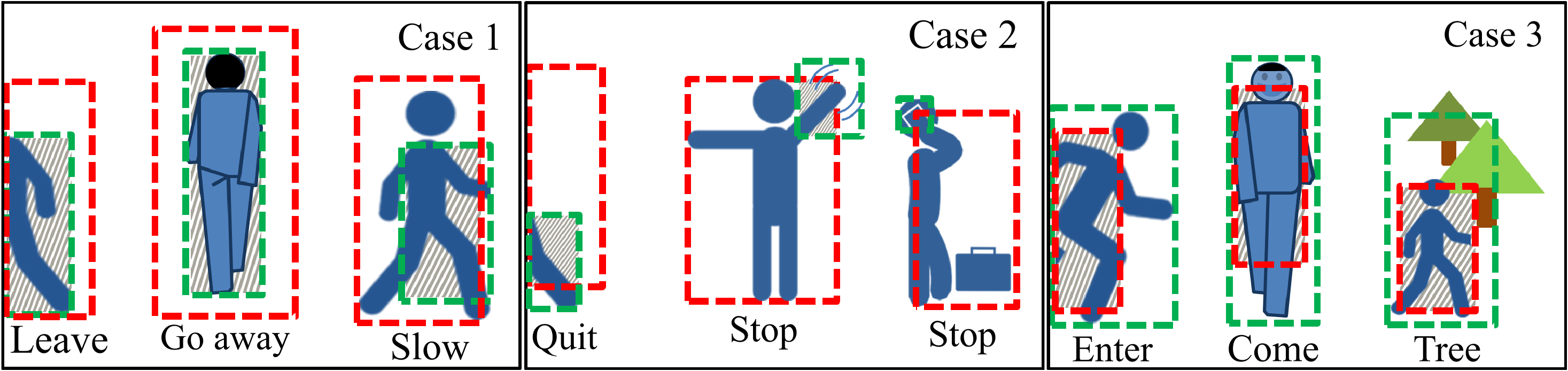
We denote the overlap box between and by . A binary variable is used to determine the final detection bounding box when is not precise. We illustrate the three possible cases of situation in Fig. 8, where Case 1 denotes that the area of measurement gets smaller, Case 2 denotes that the area gets too smaller, and Case 3 denotes that the area is growing. We summarize the refinement process in Fig. 9 and provide the details in the following.

- •
Case 1: and
If the moving object leaves the screen or is undergoing motion along the z-axis, we consider to be precise and let . Otherwise, we can adopt the refined bounding box as and set .
- •
Case 2: and
When the detected object moves out of the screen, we consider to be precise and adopt ; otherwise, the object remains in stasis. We refine the bounding box as and set .
- •
Case 3: and
If the object undergoes motion along the z-axis towards the camera or enters the field of view, we consider is precise and set . Otherwise, the initial detected bounding box may be merged with background noise, such as noise from trees. We employ the refined bounding box as and set .
- •
Otherwise:
If and are too small, the estimation and the observation are too mismatched that we have to discard them both. We refine the bounding box as
(37) If , we set ; otherwise, we set .
The refined measurement vector is computed as . At each iteration, is passed as feedback to Eq. (20) in the update process, and the subsequent Kalman filtering process is continued. If is precise, the final detected bounding box can be formulated as
| (38) |
where denotes the bounding box determined by the posteriori estimate , i.e., . Otherwise, the detected bounding box is obtained as
| (39) |
3.3.4 Occlusion Problem
The occlusion here means multiple objects are obscured, resulting in their clusters connected in the feature image. It is difficult to split them in the encrypted and compressed domain. Because the time interval of two adjacent frames is very short, it is reasonable to assume that the velocities and the sizes of the bounding boxes of the occluded objects remain unchanged during the occlusion. In the -th frame, we first compute all the mean size box s. For every object, we delete the points in the feature image that do not belong to or , and then restore the points in the to obtain a new feature image . We perform the clustering algorithm on and denote the rectangle generated from the biggest cluster as . If , we let , otherwise we let . The final detected bounding box is .
4 Experimental Results
In our experiments, we mainly considered surveillance scenarios with low crowd densities, since they are typical of real-world monitoring scenarios with privacy concerns, such as in the home or laboratory. Our experimental database consisted of 16 video sequences selected from four video data sets: LASIESTA (Cuevas et al. 2016), CWD-2014 (Goyette et al. 2012), OTCBVS (Davis and Sharma 2007), and CAVIAR (Fisher et al. 2004). These videos contain critical challenges in detection, and we list them in Table 1. Since OTCBVS and CAVIAR contain only bounding box ground truths, we used them in the experiments on motion tracking.
| Dataset | Frames |
|
Resolution | Challenges | ||||
|---|---|---|---|---|---|---|---|---|
| LASIESTA | 3931 | 10 | 352*288 |
| ||||
| CDW-2014 | 800 | 1 | 360*240 |
| ||||
| OTCBVS | 3068 | 2 | 320*240 |
| ||||
| CAVIAR | 2842 | 3 | 384*288 |
|
| Method | Pr | Re | F1 |
|---|---|---|---|
| LMVD (Guo et al. 2017) | 0.3823 | 0.9154 | 0.4940 |
| CB+PD (Ma et al. 2018) | 0.4980 | 0.8354 | 0.6148 |
| DNRC (proposed) | 0.6132 | 0.8655 | 0.7083 |

Video name DNRC (proposed) LMVD (Guo et al. 2017) CB+PD (Ma et al. 2018) Pr Re F1 Pr Re F1 Pr Re F1 I_BS_01 0.7059 0.8650 0.7774 0.4419 0.9517 0.6036 0.5183 0.8804 0.6525 I_BS_02 0.5319 0.7139 0.6096 0.4425 0.7270 0.5502 0.4601 0.7207 0.5616 I_MB_02 0.7350 0.6345 0.6810 0.5929 0.8849 0.7101 0.6264 0.7014 0.6617 I_MC_02 0.5326 0.9428 0.6807 0.0677 0.9890 0.1267 0.4821 0.9587 0.6416 I_SI_02 0.7269 0.8933 0.8016 0.5116 0.9349 0.6613 0.5437 0.7957 0.6460 O_CL_02 0.6009 0.9605 0.7393 0.5063 0.9341 0.6567 0.4461 0.9242 0.6017 O_MC_01 0.5686 0.9669 0.7161 0.0400 0.9972 0.0769 0.4500 0.9602 0.6128 O_RA_02 0.5452 0.9293 0.6872 0.5616 0.9056 0.6933 0.5229 0.9397 0.6719 O_SM_04 0.5107 0.9723 0.6696 0.0455 0.9952 0.0870 0.4272 0.9222 0.5839 O_SN_02 0.7036 0.7329 0.7179 0.4967 0.8261 0.6204 0.9222 0.4582 0.4785 pedestrians 0.5834 0.9087 0.7106 0.4986 0.9232 0.6475 0.5006 0.9283 0.6505 Average 0.6132 0.8655 0.7083 0.3823 0.9154 0.4940 0.4980 0.8354 0.6148
[] Algorithm Name Detector Domain Stationary Camera Moving Camera Normal Videos Encrypted Videos Normal Videos Encrypted Videos Pr Re F1 Pr Re F1 Pr Re F1 Pr Re F1 GMM(Stauffer and Grimson 1999) pixel 0.6368 0.8393 0.7104 0.0289 0.5360 0.0508 0.3325 0.7316 0.3754 0.0217 0.5133 0.0415 SC-SOBS(Maddalena and Petrosino 2012) pixel 0.7746 0.7370 0.7329 0.0300 0.8787 0.05745 0.2455 0.8528 0.3077 0.0227 0.9082 0.0441 SuBSENCE(St-Charles et al. 2015) pixel 0.9393 0.7056 0.7925 0.0425 0.1763 0.0661 0.6316 0.84597 0.6263 0.0472 0.1917 0.0737 ST-MRF(Khatoonabadi and Bajic 2013) CVB1 0.7000 0.5029 0.5584 0.6693 0.1089 0.1820 0.5547 0.72277 0.6134 0.1720 0.0804 0.0663 Bhaskar(Dey and Kundu 2013) CVB 0.6644 0.2998 0.3991 0.0377 0.3683 0.0653 0.5978 0.3878 0.3909 0.0432 0.3636 0.0722 Zhao(Zhao et al. 2018) CVB 0.5283 0.8224 0.6394 0.1842 0.7022 0.2816 0.0685 0.9595 0.1244 0.0325 0.95393 0.0624 LMVD(Guo et al. 2017) CVB 0.5065 0.8859 0.6429 0.50651 0.88594 0.6429 0.0511 0.9938 0.0969 0.0511 0.9938 0.0969 CB+PD(Ma et al. 2018) CVB 0.5149 0.7936 0.6155 0.51485 0.79356 0.6155 0.4531 0.94703 0.6127 0.4531 0.94703 0.6127 DNRC(proposed) CVB 0.6434 0.8298 0.7167 0.64339 0.82976 0.7167 0.5405 0.9606 0.6915 0.5405 0.9606 0.6915 1 Compressed Video Bitstream
We implemented the proposed encryption scheme using the H.264/AVC reference software JM-19.0. We used the high profile with the GOP structure of IPPP. All the video sequences were encoded at 30 frames per second with an intra-period of 12 and a fixed quantization step parameter of 28. All the experiments were carried out on a 64-bit Windows 7 PC with a 3.40 GHz Intel Core i7-6700 CPU and 32 GB RAM. As discussed in (Milan et al. 2016), the overlap rate of a match is at least 0.5. Thus, we set and to obtain a more credible tracking result, and it can be inferred that . We also set frames for the experiments.
4.1 Performance of Motion Segmentation

In general, the performance of motion segmentation is evaluated based on the metrics of precision (Pr), recall (Re), and F1-score (F1) (Goyette et al. 2012). We compared the segmentation performance of our scheme with other existing schemes (Guo et al. 2017; Ma et al. 2018) on encrypted video. The scheme proposed by Ma et al. (Ma et al. 2018) was modified to use H.264/AVC. The experimental results are shown in Table 3, where it can be seen that our proposed scheme outperformed the other existing schemes on encrypted and compressed video. Our scheme achieved superior results for precision and F1-score. Although Guo’s scheme (Guo et al. 2017) had a higher score for average recall, it contained too many false detections in complex scenarios. The main reason for this is that moving cameras and dynamic backgrounds can make it challenging to distinguish noise motion vectors from the foregrounds. However, using the proposed feature, we can easily reduce the background noise. Because the motion of the camera and the presence of a dynamic background usually cause small and scattered DNRCs. All of the average values of the segmentation metrics with DNRC were better than those with CB and PD (CB+PD). Since the finest scale of our feature is 44 block level, compared to 1616 block level for Ma’s and Guo’s features, our scheme gives more precise segmentation results. A comparison of several examples of segmentation results is given in Fig. 10. Guo’s method shows apparent regions of noise in the O_MC_01 and O_SM_04 sequences. In Ma’s method, the edges of the object regions are rough, and there are many false detections around the object. In contrast, we can see that our algorithm can accurately detect moving objects without including an additional noise cluster region. Most regions are classified correctly, and only a few red and blue pixels are seen at the edges of the objects.
| Method | AUC | Pre20 | MOTA | MOTP |
|---|---|---|---|---|
| LMVD (Guo et al. 2017) | 0.3688 | 0.6658 | -0.1601 | 0.6324 |
| CB+PD (Ma et al. 2018) | 0.4307 | 0.7972 | -0.0210 | 0.6613 |
| DNRC (proposed) | 0.6633 | 0.9544 | 0.7230 | 0.7100 |


Video name Proposed Guo (Guo et al. 2017) Ma (Ma et al. 2018) AUC Pre20 MOTA MOTP AUC Pre20 MOTA MOTP AUC Pre20 MOTA MOTP I_BS_01 0.7196 0.9149 0.7957 0.7622 0.1344 0.3510 -0.6271 0.5686 0.6127 0.9338 0.6027 0.6698 I_BS_02 0.6428 0.8657 0.5865 0.7264 0.4843 0.9921 -0.0079 0.5831 0.6722 1.0000 0.7377 0.7060 I_MB_02 0.6002 0.6161 0.4554 0.6903 0.3588 0.6463 -0.7235 0.5681 0.6722 0.7243 0.8131 0.7030 I_MC_02 0.6617 0.7938 0.6495 0.7192 0.0722 0.0741 -3.7800 0.0000 0.6157 0.9575 0.6170 0.7032 I_SI_02 0.7781 0.9755 0.9406 0.7995 0.4034 0.9340 -0.3251 0.6715 0.4987 0.9754 0.0148 0.6380 O_CL_02 0.7487 0.9977 0.9400 0.7589 0.3901 0.7082 -0.0871 0.6861 0.5559 1.0000 0.2554 0.6553 O_MC_01 0.6821 0.9744 0.8564 0.7101 0.0112 0.0088 -2.8214 0.6291 0.5249 0.9893 0.2366 0.6232 O_RA_02 0.7082 0.9097 0.7208 0.7639 0.6281 0.9595 0.7432 0.6821 0.6530 0.9608 0.7124 0.7114 O_SM_04 0.5996 0.9661 0.4621 0.6973 0.0328 0.0166 -1.8031 0.5688 0.5564 0.9933 0.2953 0.6499 O_SN_02 0.6398 1.0000 0.6356 0.6791 0.4761 0.9739 -0.0970 0.5834 0.0000 0.0000 0.0000 0.0000 pedestrians 0.6916 0.9603 0.7339 0.7401 0.3556 0.5740 0.1754 0.6514 0.6215 0.9866 0.5898 0.6786 4b 0.5917 1.0000 0.5575 0.6368 0.5066 0.9953 0.0651 0.6249 0.3110 1.0000 -0.9932 0.5293 6b 0.6642 0.9882 0.8660 0.6898 0.5548 0.9885 0.4163 0.6258 0.2926 0.7708 -0.5701 0.5334 OSNE1f 0.6025 1.0000 0.5467 0.6641 0.5303 0.9719 0.2303 0.6082 0.4590 0.8554 -0.05421 0.6162 WBS1f 0.7128 0.9614 0.8491 0.7435 0.6078 0.8540 0.5752 0.6519 0.3030 0.3580 -0.2585 0.6888 OLSR1c 0.6612 0.9059 0.6849 0.7163 0.3192 0.6618 -0.7344 0.5793 0.3859 0.4927 0.0027 0.6481 Overall 0.6633 0.9544 0.7230 0.7100 0.3688 0.6658 -0.1601 0.6324 0.4307 0.7972 -0.0210 0.6613
We also compare our scheme with some previous methods (Zhao et al. 2018; Guo et al. 2017; Ma et al. 2018; Stauffer and Grimson 1999; Maddalena and Petrosino 2012; St-Charles et al. 2015; Khatoonabadi and Bajic 2013; Dey and Kundu 2013) on encrypted and unencrypted videos. As some methods are only suitable for stationary backgrounds, the videos in our dataset were divided into two categories, with stationary and moving cameras. Since the encrypted domain feature remains unchanged after encryption, algorithms based on this can obtain the same segmentation results on encrypted videos as on the original videos. We evaluated the segmentation results pixel by pixel rather than block by block, and the experimental results are given in Table 4. To our best knowledge, it is impossible to separate a moving object from the background at the pixel scale with a compressed-domain based method. That is because all of the available features extracted from bitstreams have a minimum scale of 44 pixels. Therefore, pixel-domain-based methods generally outperform compressed-domain-based methods on unencrypted video, except that our method achieved the best F1 performance for unencrypted videos with moving cameras. However, the performance of pixel-domain-based methods is sharply reduced when dealing with encrypted video. Although Guo’s scheme obtained the best recall performance for encrypted video with stationary cameras, it ultimately failed to detect objects in videos with moving cameras (). Generally, our scheme has the best F1 performance on encrypted videos among all the compared methods, whenever the camera is stationary or moving.
Our performance can catch up with that of some pixel-based methods owing to the proposed DNRC feature and the proposed refinement method. Take GMM (Stauffer and Grimson 1999) as an example of pixel-based methods. GMM needs to model the background and then find motion regions based on local pixel changes. Since any pixel change will be reflected in residual data, DNRC can also well reflect where the motion regions are. Besides, some video sequences do not leave sufficient initial frames for background modeling of GMM when the objects are moving from the first frame. It results in that GMM detects a “ghost” and thus performs poorly in these video sequences. Two examples of “ghost” are shown in Fig. 13. We can also see that GMM leaves a “ghost” when the background object of the backpack is removed. As for the proposed refinement method, it is used to adaptively update the measured bounding boxes before feeding them into the Kalman-filtering based motion model. It helps the detector to focus on the candidate motion regions to achieve better clustering results and then improve the detection performance.


4.2 Performance of Motion Detection and Tracking
Many previous studies of 2D view-based online object detection and tracking schemes have used success and precision plots to evaluate these schemes against an object tracking benchmark (Wu et al. 2013). A success plot measures the bounding box overlap, while a precision plot measures the central location error. Besides these two measures, we also evaluate the detection and tracking performance using two famous metrics in (Milan et al. 2016): multiple object tracking accuracy (MOTA) and multiple object tracking precision (MOTP). In MOTA and MOTP, the overlap rate of a match is at least 0.5.
We ran a one-pass evaluation (OPE) (Wu et al. 2013) from the first frame to the end, since no initialization was used in our moving object tracking task. Because motion detection and tracking methods based on the pixel domain do not work in our privacy-preserving application scenario, we only carried out a comparison between schemes (Guo et al. 2017; Ma et al. 2018) designed for the encrypted and compressed domain. Some videos in the databases did not contain ground truth bounding boxes (GT-boxes). We then generated the GT-boxes by drawing the minimum rectangular boxes necessary to bound the objects, strictly respecting the segmentation ground truth in each frame.
The experimental results of motion detection and tracking on encrypted videos are given in Table 6. Our scheme showed comparable performance for all videos and achieved the best average values for each metric than the other existing methods. We also plotted the tracking boxes and trajectories in the unencrypted frames to visualize the tracking results, and some examples are shown in Fig. 12. Guo’s method performed poorly for all videos with a moving camera, due to incorrect detection of background noise. The inferior trajectory results indicate that this method does not work in complex scenarios. Ma’s scheme also failed to track objects in some videos such as O_SN_02 and OLSR1r. In Ma’s method, small-sized objects are hard to detect with 1616 block-level features, and short trajectories are discarded. Additionally, the trajectories generated by Ma’s scheme contain more fluctuations, meaning that this scheme is unstable. In contrast, our method can effectively detect small-sized objects and have robust tracking performance on all encrypted videos.


Encryption Scheme Codec Format Motion Segmentation Motion tracking Precision Recall F1-score AUC PRE20 MOTA MOTP Xu (Xu et al. 2014) H.264/AVC 0.6132 0.8655 0.7083 0.6633 0.9544 0.7230 0.7100 Shahid (Shahid et al. 2011) H.264/AVC 0.6132 0.8655 0.7083 0.6633 0.9544 0.7230 0.7100 Sallam (Sallam et al. 2018) H.265/HEVC 0.6435 0.8374 0.7178 0.6733 0.8908 0.6930 0.7402 Shahid (Shahid and Puech 2014) H.265/HEVC 0.6435 0.8374 0.7178 0.6733 0.8908 0.6930 0.7402
We also illustrate our scheme’s tracking performance in terms of handling an occlusion challenge using two examples, as shown in Fig. 15. Although most regions of the occluded object are obscured by another moving object, the proposed algorithm can assign their IDs correctly and track them properly. Thus, our scheme allows for reliable tracking of the detected objects even under occlusion.
To further demonstrate the detection and tracking performance of our scheme, Fig. 14 shows success and precision plots for all videos in comparison with the other methods. These results show that the detection and tracking performance of the proposed algorithm is significantly better than the other tracking methods.
4.3 Performance on High-Definition Video
The proposed feature has the advantage of detecting more tiny objects from HD surveillance video and therefore obtains a good performance. We conducted HD video experiments to compare the performance between our 44 feature and 1616 features. To get a residual feature with a scale of 1616 pixels, we extract the number of non-zero residual coefficients in a macroblock, denoted as DNRC_MB. We also compare with LMVD (Guo et al. 2017) and CB+PD (Ma et al. 2018). Some snippets with 19201080 resolution from VIRAT (Oh et al. 2011) are used for testing. The experimental results are summarized in Table 8. We can see that our 44 feature performs better than all the compared 1616 features for HD videos.
| Feature Name | AUC | PRE20 | MOTA | MOTP |
|---|---|---|---|---|
| DNRC (proposed) | 0.6202 | 0.9802 | 0.4688 | 0.6883 |
| DNRC_MB | 0.5878 | 0.9520 | 0.3375 | 0.6691 |
| LMVD (Guo et al. 2017) | 0.4695 | 0.7799 | 0.3856 | 0.6472 |
| CB+PD (Ma et al. 2018) | 0.5636 | 0.9318 | 0.4515 | 0.6360 |
5 Discussions
5.1 Explanation of the Proposed Feature
In video encoding frameworks, prediction and compensation technologies are widely adopted to reduce spatial and temporal redundancies. In general, the pixel values in the background area are similar, since most of the background is smooth, without a complicated context. Therefore, the prediction of the background will result in small residues of blocks in the background regions. However, in a video with a moving camera, the compensation for this motion can significantly reduce the amount of residual data. In contrast, the moving object region has a more sophisticated level of detail. The pixel values in the moving object region change rapidly, reflecting the object’s motion, which cannot be predicted by the video encoder. Thus, the prediction and compensation of the moving object regions will require a more significant amount of residual data to represent the details and the unexpected motion. As a measure of the amount of residual data, the proposed DNRC feature can reflect the moving object region.
We used 10,324 labeled frames (except I frame) to analyze the raw DNRC data’s statistical characteristics and show the results in Fig. 16. The curve of DNRC distribution shows a decreasing trend, while the probability curve shows an increase. The bar at the abscissa of 16 also includes the number of blocks whose DNRCs are greater than 16. Due to a large number of background blocks, the number of blocks with a zero DNRC value account for a significant proportion (about 96%). The probability of these blocks being motion blocks is merely about 1%. Therefore, we focus only on blocks with non-zero DNRCs. Based on the tendency of the curve in Fig. 16, we can conclude that a larger DNRC block has a higher probability of being a motion block.

5.2 Running Time
Without fully decoding or any decryption, we can extract the DNRC feature directly from video bitstreams, which is very cost-effective in terms of time. The average processing speed of our scheme for all videos reaches 107.92 fps, meaning that it is highly efficient and satisfies the requirements of real-time processing. The main factor contributing to this high speed is that the DNRC feature can be efficiently extracted and processed with no complicated calculations of the pixel values, as in optical flow.
5.3 Impact of Parameter
Only one manual parameter is used in the proposed scheme, i.e., the time-domain filter parameter . We conducted experiments to investigate the sensitivity of the performance on the value of the manual parameter. We vary the value of from 3 to 9 and then compute the average F1-score of object detection for all video sequences. The results are shown in Fig. 17, from which we can see that the chosen of from common values has a small influence on our scheme’s performance.
To investigate the reality of the assumption, i.e., there is one noise spike approximately every frames. We have conducted experiments on the statistical distribution of noise spikes in the test video dataset. We show an example in Fig. 18. Every frames only contain one or two noise spikes. Our experimental results show that this assumption is reasonable in the scenario of video surveillance.
5.4 Extension to other Video Coding Standards and Video Bitstream Encryption Schemes
The proposed technique for object tracking is not specifically designed to rely on the H.264 video encryption scheme in this paper. We can adapt the proposed scheme to other advanced video encoding frameworks, such as H.265 video compression, since residual data widely exist in these video compression standards. The proposed detection and tracking scheme is also applicable to other video bitstream encryption methods. We have conducted more experiments to investigate the effectiveness of our scheme on four different H.264/H.265 video encryptions (Xu et al. 2014; Shahid et al. 2011; Sallam et al. 2018; Shahid and Puech 2014). As shown in Table 7, the experimental results demonstrate that the proposed motion detection and tracking technique also works for these tested video encryption schemes. Note that the extracted DNRC features from two different encryption schemes under the same codec are the same. Our motion and tracking scheme achieves the same performances under the same codec.
5.5 Analysis of Privacy Protection
We conducted experiments to investigate the performance of privacy protection with our video encryption under the threat models T1 and T3 (Hao et al. 2020). T1 assumes the attacker has no information of any obscuration method while T3 assumes the attacker knows the exact type of the obscuration method and its hyperparameter. We make all experimental settings to be consistent with (Hao et al. 2020). The used datasets in (Hao et al. 2020) include FaceScrub dataset (Ng and Winkler 2014) and LFW dataset (Huang et al. 2007), which are encoded into video bitstreams for our video encryption. Three types of attacks are used for examining the robustness of the employed video encryption scheme, including face identification attack, face verification attack, and face reconstruction attack. Two popular models of VGG-19 (Simonyan and Zisserman 2014) and ResNet-50 (He et al. 2016) are adopted as the model backbone. The performance of identification and verification attack are evaluated by Top 1 accuracy and AUC of ROC, respectively. Mean square error (MSE) between the clear and reconstructed image and identification accuracy of recovered images are adopted as the evaluation metrics for reconstruction attack. The experimental results are given in Table 9.
The identification accuracies of our video encryption under T1 with two backbones are less than 0.009. Under T3, the identification accuracies of the employed video encryption of two backbones are less than 0.18. Compared with other obscured methods under T3, the performance of the employed encryption scheme significantly outperforms the traditional obscuration methods and privacy-preserving image encryption methods, and is closer to that of -same based obscuration methods. For the face verification attack under T3, our video encryption with VGG-19 achieves an AUC of 0.646, which are smaller than the original -same method (Gross et al. 2006) but greater than those of -same-net (Meden et al. 2018) and UP-GAN (Hao et al. 2019). In general, the average AUC value of our video encryption are at the same level as those of the -same based methods. As for the face reconstruction attack, our video encryption achieves the highest MSE and the lowest identification accuracy. Thus, the employed encryption scheme performs better than the -same based obscuration methods in resisting reconstruction attack. According to the experimental results of the above three types of face attacks, the employed video encryption achieves a similar privacy level with the best methods in (Hao et al. 2020), i.e., the k-same based obscuration methods. Therefore, we can draw the conclusion that the employed video encryption scheme can achieve a considerable obscuration performance even under the strongest attack model T3.
For privacy protection, it is not necessary to encrypt every bit of video stream. For example, the -same obscuration methods, which were reported to be able to provide secured privacy protection for face images in (Hao et al. 2020), are also not conventional encryption schemes. According to the conventional video compression standards, e.g., H.264 and H.265, identifiable information such as human faces is relative to the intra-frame video coding. In contrast, the motion information is connected to inter-frame video coding. Thus, privacy protection and motion detection are not mutually exclusive in our application scenario of video surveillance. Specifically, from the above experimental results, we can learn that the employed video encryption has a similar face obscuration performance with the best methods in (Hao et al. 2020).
| Method | Accuracy of Identification Attack | AUC ROC of Verification Attack | Reconstruction Attack | |||||||
| VGG19 | ResNet50 | VGG19 | ResNet50 | |||||||
| T1 | T3 | T1 | T3 | T1 | T3 | T1 | T3 | MSE | Acc | |
| Clear | 0.838 | 0.886 | 0.890 | 0.884 | 0.983 | 0.983 | 0.981 | 0.981 | 0.000 | 0.849 |
| Gaussian† | 0.007 | 0.811 | 0.009 | 0.798 | 0.512 | 0.893 | 0.629 | 0.962 | 0.002 | 0.367 |
| Median† | 0.011 | 0.805 | 0.014 | 0.798 | 0.539 | 0.877 | 0.592 | 0.933 | 0.007 | 0.102 |
| Pixelation† | 0.004 | 0.373 | 0.002 | 0.323 | 0.505 | 0.630 | 0.530 | 0.792 | 0.031 | 0.006 |
| k-same‡ | 0.012 | 0.050 | 0.012 | 0.063 | 0.573 | 0.695 | 0.580 | 0.768 | 0.029 | 0.005 |
| k-same-net‡ | 0.091 | 0.095 | 0.081 | 0.092 | 0.505 | 0.497 | 0.493 | 0.492 | 0.064 | 0.018 |
| UP-GAN‡ | 0.091 | 0.093 | 0.082 | 0.088 | 0.500 | 0.494 | 0.499 | 0.497 | 0.059 | 0.003 |
| P3* | 0.001 | 0.678 | 0.002 | 0.579 | 0.503 | 0.524 | 0.502 | 0.899 | 0.013 | 0.339 |
| Scrambling* | 0.002 | 0.784 | 0.002 | 0.750 | 0.544 | 0.951 | 0.549 | 0.928 | 0.018 | 0.042 |
| Ours | 0.007 | 0.172 | 0.009 | 0.179 | 0.585 | 0.646 | 0.575 | 0.625 | 0.427 | 0.001 |


6 Conclusions
In this paper, we propose a secure and robust motion detection and object tracking scheme based on a new feature, to tackle complex and dynamic scenes in real surveillance tasks. The proposed feature DNRC is extracted from compressed video bitstream directly without decryption and full decompression. By outsourcing the detection and tracking tasks to the cloud, we can obtain responses for the moving object regions from the cloud that processes the encrypted and compressed videos. Meanwhile, the cloud can provide automatic services of effective small-sized object detection, robust and reliable detected object tracking in complex surveillance scenarios such as occlusion, camera moving, shadow, etc. Our experimental results show that the proposed scheme achieves outstanding performance in moving object detection and tracking in the encrypted domain. The proposed algorithm has good compatibility both on encryption schemes and recent codecs and can overcome the various challenges of motion detection and tracking systems in real-time.
References
- Lagendijk et al. [2013] R. L. Lagendijk, Z. Erkin, and M. Barni. Encrypted signal processing for privacy protection: Conveying the utility of homomorphic encryption and multiparty computation. IEEE Signal Process. Mag., 30(1):82–105, 2013. doi:10.1109/MSP.2012.2219653.
- Paillier [1999] Pascal Paillier. Public-key cryptosystems based on composite degree residuosity classes. In Proc. 17th Int. Conf. Theory & Appl. Cryptographic Techn., pages 223–238. Springer, 1999. ISBN 978-3-540-48910-8.
- Brakerski et al. [2014] Zvika Brakerski, Craig Gentry, and Vinod Vaikuntanathan. (Leveled) fully homomorphic encryption without bootstrapping. ACM Trans. Comput. Theory, 6(3), 2014. ISSN 1942-3454. doi:10.1145/2633600.
- Zheng and Huang [2013] Peijia Zheng and Jiwu Huang. An efficient image homomorphic encryption scheme with small ciphertext expansion. In Proc. ACM MM, pages 803–812, 2013.
- Erkin et al. [2009] Zekeriya Erkin, Martin Franz, Jorge Guajardo, Stefan Katzenbeisser, Inald Lagendijk, and Tomas Toft. Privacy-preserving face recognition. In Proc. Int. Symp. Privacy Enhancing Techn. Symp., pages 235–253. Springer, 2009. ISBN 978-3-642-03168-7.
- Troncoso-Pastoriza et al. [2013] J. R. Troncoso-Pastoriza, D. González-Jiménez, and F. Pérez-González. Fully private noninteractive face verification. IEEE Trans. Inf. Forensics Security, 8(7):1101–1114, 2013. doi:10.1109/TIFS.2013.2262273.
- Hu et al. [2016] S. Hu, Q. Wang, J. Wang, Z. Qin, and K. Ren. Securing SIFT: Privacy-preserving outsourcing computation of feature extractions over encrypted image data. IEEE Trans. Image Process., 25(7):3411–3425, 2016. doi:10.1109/TIP.2016.2568460.
- Hu et al. [2016] Xianjun Hu, Weiming Zhang, Ke Li, Honggang Hu, and Nenghai Yu. Secure nonlocal denoising in outsourced images. ACM Trans. Multimedia Comput. Commun. Appl., 12(3), March 2016. ISSN 1551-6857. doi:10.1145/2886777.
- Xiang and Luo [2018] S. Xiang and X. Luo. Reversible data hiding in homomorphic encrypted domain by mirroring ciphertext group. IEEE Trans. Circuits Syst. Video Technol., 28(11):3099–3110, 2018. doi:10.1109/TCSVT.2017.2742023.
- Zhang et al. [2016] X. Zhang, J. Long, Z. Wang, and H. Cheng. Lossless and reversible data hiding in encrypted images with public-key cryptography. IEEE Trans. Circuits Syst. Video Technol., 26(9):1622–1631, 2016. doi:10.1109/TCSVT.2015.2433194.
- Zheng et al. [2019] S. Zheng, Y. Wang, and D. Hu. Lossless data hiding based on homomorphic cryptosystem. IEEE Trans. Depend. Sec. Comput., pages 1–1, 2019. doi:10.1109/TDSC.2019.2913422.
- Duncan and Chou [1992] James H Duncan and Tsai-Chia Chou. On the detection of motion and the computation of optical flow. IEEE Trans. Pattern Anal. Mach. Intell., (3):346–352, 1992.
- Stauffer and Grimson [1999] C. Stauffer and W. E. L. Grimson. Adaptive background mixture models for real-time tracking. In Proc. CVPR, volume 2, pages 246–252 Vol. 2, 1999. doi:10.1109/CVPR.1999.784637.
- Maddalena and Petrosino [2012] L. Maddalena and A. Petrosino. The SOBS algorithm: What are the limits? In Proc. IEEE Comput. Soc. Conf. Comput. Vision & Pattern Recognit. Workshops, pages 21–26, 2012. doi:10.1109/CVPRW.2012.6238922.
- St-Charles et al. [2015] P. St-Charles, G. Bilodeau, and R. Bergevin. SuBSENSE: A universal change detection method with local adaptive sensitivity. IEEE Trans. Image Process., 24(1):359–373, 2015. doi:10.1109/TIP.2014.2378053.
- Ren et al. [2017] S. Ren, K. He, R. Girshick, and J. Sun. Faster R-CNN: Towards real-time object detection with region proposal networks. IEEE Trans. Pattern Anal. Mach. Intell., 39(6):1137–1149, 2017. doi:10.1109/TPAMI.2016.2577031.
- Redmon et al. [2016] Joseph Redmon, Santosh Divvala, Ross Girshick, and Ali Farhadi. You only look once: Unified, real-time object detection. In Proc. CVPR, June 2016.
- Khatoonabadi and Bajic [2013] S. H. Khatoonabadi and I. V. Bajic. Video object tracking in the compressed domain using spatio-temporal Markov random fields. IEEE Trans. Image Process., 22(1):300–313, 2013. doi:10.1109/TIP.2012.2214049.
- Dey and Kundu [2013] B. Dey and M. K. Kundu. Robust background subtraction for network surveillance in H.264 streaming video. IEEE Trans. Circuits Syst. Video Technol., 23(10):1695–1703, 2013. doi:10.1109/TCSVT.2013.2255416.
- Zhao et al. [2018] L. Zhao, Z. He, W. Cao, and D. Zhao. Real-time moving object segmentation and classification from HEVC compressed surveillance video. IEEE Trans. Circuits Syst. Video Technol., 28(6):1346–1357, 2018. doi:10.1109/TCSVT.2016.2645616.
- Upmanyu et al. [2009] M. Upmanyu, A. M. Namboodiri, K. Srinathan, and C. V. Jawahar. Efficient privacy preserving video surveillance. In Proc. ICCV, pages 1639–1646, 2009. doi:10.1109/ICCV.2009.5459370.
- Zeng et al. [2010] Yi-Chong Zeng, Chao-Yung Hsu, Yi-Fei Luo, Hon-Yue Chou, and Hong-Yuan Mark Liao. Object detection in encryption-based surveillance system. Proc. APSIPA Annu. Summit & Conf., pages 86–94, 2010.
- Chu et al. [2013] Kuan-Yu Chu, Yin-Hsi Kuo, and Winston H. Hsu. Real-time privacy-preserving moving object detection in the cloud. In Proc. ACM MM, page 597–600, 2013. ISBN 9781450324045. doi:10.1145/2502081.2502157.
- Jin et al. [2016] Xin Jin, Kui Guo, Chenggen Song, Xiaodong Li, Geng Zhao, Jing Luo, Yuzhen Li, Yingya Chen, Yan Liu, and Huaichao Wang. Private video foreground extraction through chaotic mapping based encryption in the cloud. In Proc. Int. Conf. Multimedia Model., pages 562–573. Springer, 2016. ISBN 978-3-319-27671-7.
- Lin et al. [2017] Chih-Yang Lin, Kahlil Muchtar, Jia-Ying Lin, Yu-Hsien Sung, and Chia-Hung Yeh. Moving object detection in the encrypted domain. Multimedia Tools & Appl., 76(7):9759–9783, 2017.
- Stutz and Uhl [2012] T. Stutz and A. Uhl. A survey of H.264 AVC/SVC encryption. IEEE Trans. Circuits Syst. Video Technol., 22(3):325–339, 2012. doi:10.1109/TCSVT.2011.2162290.
- Guo et al. [2017] Jianting Guo, Peijia Zheng, and Jiwu Huang. An efficient motion detection and tracking scheme for encrypted surveillance videos. ACM Trans. Multimedia Comput. Commun. Appl., 13(4), September 2017. ISSN 1551-6857. doi:10.1145/3131342.
- Wiegand et al. [2003] T. Wiegand, G. J. Sullivan, G. Bjontegaard, and A. Luthra. Overview of the H. 264/AVC video coding standard. IEEE Trans. Circuits Syst. Video Technol., 13(7):560–576, 2003. doi:10.1109/TCSVT.2003.815165.
- Xu et al. [2014] D. Xu, R. Wang, and Y. Q. Shi. Data hiding in encrypted H. 264/AVC video streams by codeword substitution. IEEE Trans. Inf. Forensics Security, 9(4):596–606, 2014. doi:10.1109/TIFS.2014.2302899.
- Ma et al. [2018] X. Ma, H. Peng, H. Jin, and B. Zhu. Privacy-preserving cloud-based video surveillance with adjustable granularity of privacy protection. In Proc. ICIP, pages 4133–4137, 2018. doi:10.1109/ICIP.2018.8451279.
- Shahid and Puech [2014] Z. Shahid and W. Puech. Visual protection of HEVC video by selective encryption of CABAC binstring. IEEE Multimedia, 16(1):24–36, 2014. doi:10.1109/TMM.2013.2281029.
- Sullivan et al. [2012] G. J. Sullivan, J. Ohm, W. Han, and T. Wiegand. Overview of the high efficiency video coding (HEVC) standard. IEEE Trans. Circuits Syst. Video Technol., 22(12):1649–1668, 2012. doi:10.1109/TCSVT.2012.2221191.
- Ester et al. [1996] Martin Ester, Hans-Peter Kriegel, Jörg Sander, Xiaowei Xu, et al. A density-based algorithm for discovering clusters in large spatial databases with noise. In Proc. KDD, volume 96, pages 226–231, 1996.
- Hsu et al. [2012] C. Hsu, C. Lu, and S. Pei. Image feature extraction in encrypted domain with privacy-preserving SIFT. IEEE Trans. Image Process., 21(11):4593–4607, 2012. doi:10.1109/TIP.2012.2204272.
- Shahid et al. [2011] Z. Shahid, M. Chaumont, and W. Puech. Fast protection of H.264/AVC by selective encryption of CAVLC and CABAC for I and P frames. IEEE Trans. Circuits Syst. Video Technol., 21(5):565–576, 2011. doi:10.1109/TCSVT.2011.2129090.
- Telecom, ITU [2003] Telecom, ITU. Advanced video coding for generic audiovisual services. ITU-T Recommendation H. 264, 2003.
- Poppe et al. [2009] Chris Poppe, Sarah De Bruyne, Tom Paridaens, Peter Lambert, and Rik Van de Walle. Moving object detection in the H.264/AVC compressed domain for video surveillance applications. J. Vis. Commun. & Image Representation, 20(6):428 – 437, 2009. ISSN 1047-3203. doi:https://doi.org/10.1016/j.jvcir.2009.05.001.
- Sabirin and Kim [2012] H. Sabirin and M. Kim. Moving object detection and tracking using a spatio-temporal graph in H. 264/AVC bitstreams for video surveillance. IEEE Multimedia, 14(3):657–668, 2012. doi:10.1109/TMM.2012.2187777.
- Tugrul and Polat [2014] Bulent Tugrul and Huseyin Polat. Privacy-preserving inverse distance weighted interpolation. Arabian J. for Sci. & Eng., 39(4):2773–2781, 2014. ISSN 2191-4281. doi:10.1007/s13369-013-0887-4.
- Weng et al. [2006] Shiuh-Ku Weng, Chung-Ming Kuo, and Shu-Kang Tu. Video object tracking using adaptive Kalman filter. J. Vis. Commun. & Image Representation, 17(6):1190 – 1208, 2006. ISSN 1047-3203.
- Welch et al. [1995] Greg Welch, Gary Bishop, et al. An introduction to the Kalman filter, 1995.
- Li et al. [2010] X. Li, K. Wang, W. Wang, and Y. Li. A multiple object tracking method using Kalman filter. In Proc. ICIA, pages 1862–1866, 2010. doi:10.1109/ICINFA.2010.5512258.
- Cuevas et al. [2016] Carlos Cuevas, Eva María Yáñez, and Narciso García. Labeled dataset for integral evaluation of moving object detection algorithms: LASIESTA. Comput. Vision & Image Understanding, 152:103 – 117, 2016. ISSN 1077-3142. doi:https://doi.org/10.1016/j.cviu.2016.08.005.
- Goyette et al. [2012] N. Goyette, P. Jodoin, F. Porikli, J. Konrad, and P. Ishwar. Changedetection.net: A new change detection benchmark dataset. In Proc. IEEE Comput. Soc. Conf. Comput. Vision & Pattern Recognit. Workshops, pages 1–8, 2012. doi:10.1109/CVPRW.2012.6238919.
- Davis and Sharma [2007] James W Davis and V Sharma. OTCBVS benchmark dataset collection, 2007. URL http://www.cse.ohio-state.edu/otcbvs-bench.
- Fisher et al. [2004] Robert Fisher, Jose Santos-Victor, and James Crowley. CAVIAR test case scenarios, 2004. URL http://homepages.inf.ed.ac.uk/rbf/CAVIAR.
- Milan et al. [2016] Anton Milan, Laura Leal-Taixé, Ian Reid, Stefan Roth, and Konrad Schindler. MOT16: A benchmark for multi-object tracking. arXiv:1603.00831, 2016.
- Wu et al. [2013] Yi Wu, Jongwoo Lim, and Ming-Hsuan Yang. Online object tracking: A benchmark. In Proc. CVPR, June 2013.
- Sallam et al. [2018] A. I. Sallam, O. S. Faragallah, and E. M. El-Rabaie. HEVC selective encryption using RC6 block cipher technique. IEEE Multimedia, 20(7):1636–1644, 2018. doi:10.1109/TMM.2017.2777470.
- Oh et al. [2011] S. Oh et al. A large-scale benchmark dataset for event recognition in surveillance video. In CVPR 2011, pages 3153–3160, 2011. doi:10.1109/CVPR.2011.5995586.
- Hao et al. [2020] Hanxiang Hao, David Güera, János Horváth, Amy R. Reibman, and Edward J. Delp. Robustness analysis of face obscuration. In 15th IEEE Int. Conf. Autom. Face & Gesture Recognit., pages 176–183, 2020. doi:10.1109/FG47880.2020.00021.
- Ng and Winkler [2014] H. Ng and S. Winkler. A data-driven approach to cleaning large face datasets. In Proc. ICIP, pages 343–347, 2014.
- Huang et al. [2007] G. B. Huang, M. Ramesh, T. Berg, and E. Learned-Miller. Labeled faces in the wild: A database for studying face recognition in unconstrained environments. Technical Report, 2007.
- Simonyan and Zisserman [2014] Karen Simonyan and Andrew Zisserman. Very deep convolutional networks for large-scale image recognition. arXiv preprint arXiv:1409.1556, 2014.
- He et al. [2016] Kaiming He, Xiangyu Zhang, Shaoqing Ren, and Jian Sun. Deep residual learning for image recognition. In Proc. CVPR, June 2016.
- Gross et al. [2006] Ralph Gross, Edoardo Airoldi, Bradley Malin, and Latanya Sweeney. Integrating utility into face de-identification. In Proc. Int. Workshop Privacy Enhancing Technol., pages 227–242. Springer, 2006. ISBN 978-3-540-34746-0.
- Meden et al. [2018] Blaž Meden, Žiga Emeršič, Vitomir Štruc, and Peter Peer. k-same-net: k-anonymity with generative deep neural networks for face deidentification. Entropy, 20(1), 2018. ISSN 1099-4300. doi:10.3390/e20010060.
- Hao et al. [2019] Hanxiang Hao, David Güera, Amy R Reibman, and Edward J Delp. A utility-preserving gan for face obscuration. arXiv preprint arXiv:1906.11979, 2019.