2 Trigonometric shearlets
We denote two-dimensional vectors by 𝐱 = ( x 1 , x 2 ) T \mathbf{x}=(x_{1},x_{2})^{\mathrm{T}} 𝐱 T 𝐲 : = x 1 y 1 + x 2 y 2 \mathbf{x}^{\mathrm{T}}\mathbf{y}\mathrel{\mathop{:}}=x_{1}\,y_{1}+x_{2}\,y_{2} | 𝐱 | 2 : = 𝐱 T 𝐱 \left\lvert\mathbf{x}\right\rvert_{2}\mathrel{\mathop{:}}=\sqrt{\mathbf{x}^{\mathrm{T}}\mathbf{x}} | 𝐱 | 1 : = | x 1 | + | x 2 | \left\lvert\mathbf{x}\right\rvert_{1}\mathrel{\mathop{:}}=\left\lvert x_{1}\right\rvert+\left\lvert x_{2}\right\rvert 𝐱 𝐲 : = x 1 y 1 x 2 y 2 \mathbf{x}^{\mathbf{y}}\mathrel{\mathop{:}}=x_{1}^{y_{1}}\,x_{2}^{y_{2}} 𝐱 β : = x 1 β x 2 β \mathbf{x}^{\beta}\mathrel{\mathop{:}}=x_{1}^{\beta}\,x_{2}^{\beta} β ∈ ℝ \beta\in\mathbb{R} 𝝃 ∈ ℝ 2 \boldsymbol{\xi}\in\mathbb{R}^{2} 𝝃 = ρ 𝚯 ( θ ) \boldsymbol{\xi}=\rho\,\boldsymbol{\Theta}(\theta) ρ : = | 𝝃 | 2 \rho\mathrel{\mathop{:}}=\left\lvert\boldsymbol{\xi}\right\rvert_{2} 𝚯 ( θ ) : = ( cos θ , sin θ ) T \boldsymbol{\Theta}(\theta)\mathrel{\mathop{:}}=(\cos\theta,\sin\theta)^{\mathrm{T}} 𝐤 ∈ ℕ 0 2 \mathbf{k}\in\mathbb{N}_{0}^{2} n ∈ ℕ 0 n\in\mathbb{N}_{0} | 𝐤 | 1 ≤ n \left\lvert\mathbf{k}\right\rvert_{1}\leq n 𝐤 ! : = k 1 ! k 2 ! \mathbf{k}!\mathrel{\mathop{:}}=k_{1}!\,k_{2}! ( n 𝐤 ) : = n ! 𝐤 ! ( n − | 𝐤 | 1 ) ! \binom{n}{\mathbf{k}}\mathrel{\mathop{:}}=\frac{n!}{\mathbf{k}!(n-\left\lvert\mathbf{k}\right\rvert_{1})!} C ( Ω ) C(\Omega) Ω ⊆ ℝ 2 \Omega\subseteq\mathbb{R}^{2} ‖ f ‖ C ( Ω ) : = sup 𝐱 ∈ A | f ( 𝐱 ) | \left\lVert f\right\rVert_{C(\Omega)}\mathrel{\mathop{:}}=\sup\limits_{\mathbf{x}\in A}\left\lvert f(\mathbf{x})\right\rvert 𝐫 = ( r 1 , r 2 ) T ∈ ℕ 0 2 \mathbf{r}=(r_{1},r_{2})^{\mathrm{T}}\in\mathbb{N}_{0}^{2} f f ∂ 𝐫 f : = ∂ r 1 + r 2 ∂ x 1 r 1 ∂ x 2 r 2 f \partial^{\mathbf{r}}f\mathrel{\mathop{:}}=\frac{\partial^{r_{1}+r_{2}}}{\partial x_{1}^{r_{1}}\partial x_{2}^{r_{2}}}f q q
C 0 q ( Ω ) : = { f : Ω → ℝ : ∂ 𝐫 f ∈ C ( Ω ) for all 𝐫 ∈ ℕ 0 2 with | 𝐫 | 1 ≤ q , | supp f | < ∞ } C^{q}_{0}(\Omega)\mathrel{\mathop{:}}=\left\{f:\Omega\rightarrow\mathbb{R}:\partial^{\mathbf{r}}f\in C(\Omega)\;\text{for all}\;\mathbf{r}\in\mathbb{N}_{0}^{2}\;\text{with}\;\left\lvert\mathbf{r}\right\rvert_{1}\leq q,\,\left\lvert\mathrm{supp}\,f\right\rvert<\infty\right\}
with the norm ‖ f ‖ C 0 q : = ‖ f ‖ C 0 q ( Ω ) : = sup | 𝐫 | 1 ≤ q sup 𝐱 ∈ Ω | ∂ 𝐫 f ( 𝐱 ) | \left\lVert f\right\rVert_{C_{0}^{q}}\mathrel{\mathop{:}}=\left\lVert f\right\rVert_{C_{0}^{q}(\Omega)}\mathrel{\mathop{:}}=\sup\limits_{\left\lvert\mathbf{r}\right\rvert_{1}\leq q}\,\sup\limits_{\mathbf{x}\in\Omega}\left\lvert\partial^{\mathbf{r}}f(\mathbf{x})\right\rvert
In this section, we define trigonometric shearlets which were already used in [22 ] . For convenience, we briefly recap the construction and some properties of these functions.
We call a nonnegative and even function g : ℝ → ℝ g:\mathbb{R}\rightarrow\mathbb{R} supp g = ( − 2 3 , 2 3 ) \mathrm{supp}\,g=\left(-\frac{2}{3},\frac{2}{3}\right) g g x ∈ ( 1 3 , 2 3 ) x\in\left(\frac{1}{3},\frac{2}{3}\right) ∑ z ∈ ℤ g ( x + z ) = 1 \sum\limits_{z\in\mathbb{Z}}g(x+z)=1 x ∈ ℝ x\in\mathbb{R} g g [22 ] . We introduce functions g ~ : ℝ → ℝ \widetilde{g}:\mathbb{R}\rightarrow\mathbb{R} g ~ ( x ) : = g ( x 2 ) − g ( x ) \widetilde{g}(x)\mathrel{\mathop{:}}=g\left(\frac{x}{2}\right)-g(x)
For 𝔦 ∈ { 𝔥 , 𝔳 } \mathfrak{i}\in\{\mathfrak{h},\mathfrak{v}\} Ψ ( 𝔦 ) : ℝ 2 → ℝ \Psi^{(\mathfrak{i})}:\mathbb{R}^{2}\rightarrow\mathbb{R}
Ψ ( 𝔥 ) ( 𝐱 ) : = g ~ ( x 1 ) g ( x 2 ) , Ψ ( 𝔳 ) ( 𝐱 ) : = g ( x 1 ) g ~ ( x 2 ) . \Psi^{(\mathfrak{h})}(\mathbf{x})\mathrel{\mathop{:}}=\widetilde{g}(x_{1})\,g(x_{2}),\qquad\qquad\Psi^{(\mathfrak{v})}(\mathbf{x})\mathrel{\mathop{:}}=g(x_{1})\,\widetilde{g}(x_{2}). (2)
We call them window functions and write Ψ ( 𝔦 ) ∈ 𝒲 \Psi^{(\mathfrak{i})}\in\mathcal{W} g ∈ C 0 q ( ℝ ) g\in C^{q}_{0}(\mathbb{R}) Ψ ( 𝔦 ) ∈ C 0 q ( ℝ 2 ) \Psi^{(\mathfrak{i})}\in C^{q}_{0}(\mathbb{R}^{2}) Ψ ( 𝔦 ) ∈ 𝒲 q \Psi^{(\mathfrak{i})}\in\mathcal{W}^{q} j ∈ ℕ 0 j\in\mathbb{N}_{0} ℓ ∈ ℤ \ell\in\mathbb{Z} | ℓ | ≤ 2 j / 2 \left\lvert\ell\right\rvert\leq 2^{j/2}
𝐍 j , ℓ ( 𝔥 ) : = ( 2 j ℓ 2 j / 2 0 2 j / 2 ) , 𝐍 j , ℓ ( 𝔳 ) : = ( 2 j / 2 0 ℓ 2 j / 2 2 j ) \mathbf{N}_{j,\ell}^{(\mathfrak{h})}\mathrel{\mathop{:}}=\begin{pmatrix}2^{j}&\ell\,2^{j/2}\\
0&2^{j/2}\end{pmatrix},\qquad\qquad\;\mathbf{N}_{j,\ell}^{(\mathfrak{v})}\mathrel{\mathop{:}}=\begin{pmatrix}2^{j/2}&0\\
\ell\,2^{j/2}&2^{j}\end{pmatrix}
and introduce the functions
Ψ j , ℓ ( 𝔦 ) ( 𝐱 ) : = Ψ ( 𝔦 ) ( ( 𝐍 j , ℓ ( 𝔦 ) ) − T 𝐱 ) , 𝐱 ∈ ℝ 2 . \Psi^{(\mathfrak{i})}_{j,\ell}(\mathbf{x})\mathrel{\mathop{:}}=\Psi^{(\mathfrak{i})}\left(\left(\mathbf{N}_{j,\ell}^{(\mathfrak{i})}\right)^{-\mathrm{T}}\mathbf{x}\right),\qquad\mathbf{x}\in\mathbb{R}^{2}.
For 𝔦 ∈ { 𝔦 , 𝔳 } \mathfrak{i}\in\{\mathfrak{i},\mathfrak{v}\} Ψ ( 𝔦 ) ∈ 𝒲 q \Psi^{(\mathfrak{i})}\in\mathcal{W}^{q} 𝐲 ∈ 𝒫 ( 𝐍 j , ℓ ( 𝔦 ) ) \mathbf{y}\in\mathcal{P}(\mathbf{N}_{j,\ell}^{(\mathfrak{i})})
ψ j , ℓ , 𝐲 ( 𝔦 ) ( 𝐱 ) : = 2 − 3 j / 4 ∑ 𝐤 ∈ ℤ 2 Ψ j , ℓ ( 𝔦 ) ( 𝐤 ) e i 𝐤 T ( 𝐱 − 2 π 𝐲 ) , \psi_{j,\ell,\mathbf{y}}^{(\mathfrak{i})}(\mathbf{x})\mathrel{\mathop{:}}=2^{-3j/4}\sum_{\mathbf{k}\in\mathbb{Z}^{2}}\Psi^{(\mathfrak{i})}_{j,\ell}(\mathbf{k})\,\mathrm{e}^{\mathrm{i}\mathbf{k}^{\mathrm{T}}(\mathbf{x}-2\pi\mathbf{y})}, (3)
where
𝒫 ( 𝐍 j , ℓ ( 𝔥 ) ) = { 2 − j z 1 : z 1 = − 2 j − 1 , … , 2 j − 1 − 1 } × { 2 − j / 2 z 2 : z 2 = − 2 j / 2 − 1 , … , 2 j / 2 − 1 − 1 } , \displaystyle\mathcal{P}\left(\mathbf{N}_{j,\ell}^{(\mathfrak{h})}\right)=\Bigl\{2^{-j}\,z_{1}\,:\,z_{1}=-2^{j-1},\dots,2^{j-1}-1\Bigr\}\times\Bigl\{2^{-j/2}\,z_{2}\,:\,z_{2}=-2^{j/2-1},\dots,2^{j/2-1}-1\Bigr\},
𝒫 ( 𝐍 j , ℓ ( 𝔳 ) ) = { 2 − j / 2 z 1 : z 1 = − 2 j / 2 − 1 , … , 2 j / 2 − 1 − 1 } × { 2 − j z 2 : z 2 = − 2 j − 1 , … , 2 j − 1 − 1 } . \displaystyle\mathcal{P}\left(\mathbf{N}_{j,\ell}^{(\mathfrak{v})}\right)=\Bigl\{2^{-j/2}\,z_{1}\,:\,z_{1}=-2^{j/2-1},\dots,2^{j/2-1}-1\Bigr\}\times\Bigl\{2^{-j}\,z_{2}\,:\,z_{2}=-2^{j-1},\dots,2^{j-1}-1\Bigr\}.
Let f , g : ℝ → ℝ f,g:\mathbb{R}\rightarrow\mathbb{R} n n f f g g [21 , Section 4.3]
d n d x n f ( g ( x ) ) \displaystyle\frac{\mathrm{d}^{n}}{\mathrm{d}x^{n}}f(g(x)) = ∑ 𝐤 ( n 𝐤 ) f ( | 𝐤 | 1 ) ( g ( x ) ) ∏ j = 1 n ( g ( j ) ( x ) j ! ) k j \displaystyle=\sum\limits_{\mathbf{k}}\binom{n}{\mathbf{k}}\,f^{(\left\lvert\mathbf{k}\right\rvert_{1})}(g(x))\,\prod\limits_{j=1}^{n}\left(\frac{g^{(j)}(x)}{j!}\right)^{k_{j}}
= ∑ k = 1 n f ( k ) ( g ( x ) ) B n , k ( g ′ ( x ) , g ′′ ( x ) , … , g ( n − k + 1 ) ( x ) ) , \displaystyle=\sum\limits_{k=1}^{n}f^{(k)}(g(x))\,B_{n,k}\Bigl(g^{\prime}(x),g^{\prime\prime}(x),\ldots,g^{(n-k+1)}(x)\Bigr), (4)
where the sum in the first line runs over all vectors 𝐤 = ( k 1 , … , k n ) T ∈ ℕ 0 n \mathbf{k}=(k_{1},\ldots,k_{n})^{\mathrm{T}}\in\mathbb{N}_{0}^{n} ∑ i = 1 n i ⋅ k i = n \sum\limits_{i=1}^{n}i\cdot k_{i}=n B n , k B_{n,k}
∑ k = 0 n B n , k ( 1 , 1 , … , 1 ) = ∑ k = 0 n ∑ 𝐦 ( n 𝐦 ) ∏ j = 1 n − k + 1 ( j ! ) − m j = B n , \sum_{k=0}^{n}B_{n,k}(1,1,\ldots,1)=\sum\limits_{k=0}^{n}\sum\limits_{\mathbf{m}}\binom{n}{\mathbf{m}}\prod_{j=1}^{n-k+1}(j!)^{-m_{j}}=B_{n}, (5)
where B n B_{n} n n 𝐦 = ( m 1 , … , m n − k + 1 ) T ∈ ℕ 0 n − k + 1 \mathbf{m}=(m_{1},\ldots,m_{n-k+1})^{\mathrm{T}}\in\mathbb{N}_{0}^{n-k+1} ∑ i = 1 n − k + 1 m i = k \sum\limits_{i=1}^{n-k+1}m_{i}=k ∑ i = 1 n i ⋅ m i = n \sum\limits_{i=1}^{n}i\cdot m_{i}=n
θ j , ℓ ( h ) : = arctan ( ℓ 2 − j / 2 ) , θ j , ℓ ( v ) : = arccot ( ℓ 2 − j / 2 ) . \theta_{j,\ell}^{(\mathrm{h})}\mathrel{\mathop{:}}=\arctan\left(\ell\,2^{-j/2}\right),\qquad\qquad\theta_{j,\ell}^{(\mathrm{v})}\mathrel{\mathop{:}}=\mathrm{arccot}\left(\ell\,2^{-j/2}\right). (6)
Lemma 2.1 .
For 𝔦 ∈ { 𝔥 , 𝔳 } \mathfrak{i}\in\{\mathfrak{h},\mathfrak{v}\} q ∈ ℕ 0 q\in\mathbb{N}_{0} Ψ ( 𝔦 ) ∈ 𝒲 q \Psi^{(\mathfrak{i})}\in\mathcal{W}^{q} Eq. 2 r ≤ q r\leq q
| ∂ r ∂ ρ r [ Ψ j , ℓ ( 𝔦 ) ( 2 j ρ 𝚯 ( θ ) ) ] | ≤ C 1 ( r ) , | ∂ r ∂ θ r [ Ψ j , ℓ ( 𝔦 ) ( 2 j ρ 𝚯 ( θ ) ) ] | ≤ C 2 ( r ) 2 j r / 2 . \left\lvert\frac{\partial^{r}}{\partial\rho^{r}}\left[\Psi_{j,\ell}^{(\mathfrak{i})}\left(2^{j}\rho\,\boldsymbol{\Theta}(\theta)\right)\right]\right\rvert\leq C_{1}(r),\qquad\left\lvert\frac{\partial^{r}}{\partial\theta^{r}}\left[\Psi_{j,\ell}^{(\mathfrak{i})}\left(2^{j}\rho\,\boldsymbol{\Theta}(\theta)\right)\right]\right\rvert\leq C_{2}(r)\,2^{jr/2}.
Proof.
We only show the case 𝔦 = 𝔥 \mathfrak{i}=\mathfrak{h}
Ψ j , ℓ ( 𝔥 ) ( 2 j ρ 𝚯 ( θ ) ) = g ~ α ( ρ cos θ ) g α ( ρ cos θ ( 2 j / 2 tan θ − ℓ ) ) \Psi_{j,\ell}^{(\mathfrak{h})}\left(2^{j}\rho\,\boldsymbol{\Theta}(\theta)\right)=\widetilde{g}_{\alpha}\bigl(\rho\cos\theta\bigr)\,g_{\alpha}\Bigl(\rho\cos\theta\left(2^{j/2}\tan\theta-\ell\right)\Bigr)
and use the chain rule to get
| ∂ s ∂ ρ s [ g ~ α ( ρ cos θ ) ] | = | cos θ | s | g ~ α ( s ) ( ρ cos θ ) | ≤ ‖ g ~ α ‖ C s ( ℝ ) = C 1 ( s ) \left\lvert\frac{\partial^{s}}{\partial\rho^{s}}\left[\widetilde{g}_{\alpha}\bigl(\rho\cos\theta\bigr)\right]\right\rvert=\left\lvert\cos\theta\right\rvert^{s}\,\left\lvert\widetilde{g}_{\alpha}^{(s)}\bigl(\rho\cos\theta\bigr)\right\rvert\leq\left\lVert\widetilde{g}_{\alpha}\right\rVert_{C^{s}(\mathbb{R})}=C_{1}(s) (7)
for all s ≤ r s\leq r [22 , Lemma 1] it follows that
supp Ψ j , ℓ ( 𝔥 ) ( 2 j ρ 𝚯 ( θ ) ) ⊂ { ( ρ , θ ) ∈ ℝ × [ − π 2 , π 2 ] : 1 3 < | ρ | < 2 , θ j , ℓ − 2 ( 𝔥 ) < θ < θ j , ℓ + 2 ( 𝔥 ) } , \mathrm{supp}\,\Psi_{j,\ell}^{(\mathfrak{h})}\left(2^{j}\rho\,\boldsymbol{\Theta}(\theta)\right)\subset\left\{(\rho,\theta)\in\mathbb{R}\times\left[-\frac{\pi}{2},\frac{\pi}{2}\right]:\frac{1}{3}<\left\lvert\rho\right\rvert<2,\,\theta_{j,\ell-2}^{(\mathfrak{h})}<\theta<\theta_{j,\ell+2}^{(\mathfrak{h})}\right\},
leading to the estimate
| ∂ s ∂ ρ s [ g α ( ρ cos θ ( 2 j / 2 tan θ − ℓ ) ) ] | \displaystyle\left\lvert\frac{\partial^{s}}{\partial\rho^{s}}\left[g_{\alpha}\Bigl(\rho\cos\theta\left(2^{j/2}\tan\theta-\ell\right)\Bigr)\right]\right\rvert = | cos θ | s | 2 j / 2 tan θ − ℓ | s | g α ( s ) ( ρ cos θ ( 2 j / 2 tan θ − ℓ ) ) | \displaystyle=\left\lvert\cos\theta\right\rvert^{s}\Bigl\lvert 2^{j/2}\tan\theta-\ell\Bigr\rvert^{s}\left\lvert g_{\alpha}^{(s)}\Bigl(\rho\cos\theta\left(2^{j/2}\tan\theta-\ell\right)\Bigr)\right\rvert
≤ 2 s ‖ g α ‖ C s ( ℝ ) ≤ C 2 . \displaystyle\leq 2^{s}\,\left\lVert g_{\alpha}\right\rVert_{C^{s}(\mathbb{R})}\leq C_{2}. (8)
Using Leibniz rule and triangle inequality we get with Eq. 7 Section 2
| ∂ r ∂ ρ r [ Ψ j , ℓ ( 𝔥 ) ( 2 j ρ 𝚯 ( θ ) ) ] | ≤ ∑ s = 0 r ( r s ) 2 r − s C 1 ( s ) C 2 ( r − s ) ≤ 3 r C 3 ( r ) = C 4 ( r ) . \left\lvert\frac{\partial^{r}}{\partial\rho^{r}}\left[\Psi_{j,\ell}^{(\mathfrak{h})}\left(2^{j}\rho\,\boldsymbol{\Theta}(\theta)\right)\right]\right\rvert\leq\sum\limits_{s=0}^{r}\binom{r}{s}\,2^{r-s}\,C_{1}(s)\,C_{2}(r-s)\leq 3^{r}\,C_{3}(r)=C_{4}(r).
For the variable θ \theta s ≤ r s\leq r
| ∂ s ∂ θ s [ ρ cos θ ] | ≤ | ρ | , \left\lvert\frac{\partial^{s}}{\partial\theta^{s}}\left[\rho\cos\theta\right]\right\rvert\leq\left\lvert\rho\right\rvert,
which leads with Eq. 5 Eq. 4
| ∂ s ∂ θ s [ g ~ α ( ρ cos θ ) ] | \displaystyle\left\lvert\frac{\partial^{s}}{\partial\theta^{s}}\left[\widetilde{g}_{\alpha}\bigl(\rho\cos\theta\bigr)\right]\right\rvert ≤ ∑ t = 1 s | g ~ α ( t ) ( ρ cos θ ) | B s , t ( | ∂ ∂ θ [ ρ cos θ ] | , … , | ∂ s − t + 1 ∂ θ s − t + 1 [ ρ cos θ ] | ) \displaystyle\leq\sum\limits_{t=1}^{s}\left\lvert\widetilde{g}_{\alpha}^{(t)}\bigl(\rho\cos\theta\bigr)\right\rvert\,B_{s,t}\left(\left\lvert\frac{\partial}{\partial\theta}\left[\rho\cos\theta\right]\right\rvert,\ldots,\left\lvert\frac{\partial^{s-t+1}}{\partial\theta^{s-t+1}}\left[\rho\cos\theta\right]\right\rvert\right)
≤ ‖ g ~ α ‖ C s ( ℝ ) ∑ t = 1 s ∑ 𝐦 ( s 𝐦 ) ∏ j = 1 s − t + 1 ( | ∂ j ∂ θ j [ ρ cos θ ] | j ! ) m j \displaystyle\leq\left\lVert\widetilde{g}_{\alpha}\right\rVert_{C^{s}(\mathbb{R})}\sum\limits_{t=1}^{s}\sum\limits_{\mathbf{m}}\binom{s}{\mathbf{m}}\prod_{j=1}^{s-t+1}\left(\frac{\left\lvert\frac{\partial^{j}}{\partial\theta^{j}}\left[\rho\cos\theta\right]\right\rvert}{j!}\right)^{m_{j}}
≤ C 5 ( s ) ∑ t = 1 s | ρ | t ∑ 𝐦 ( s 𝐦 ) ∏ j = 1 s − t + 1 ( j ! ) − m j ≤ C 6 ( s ) B s = C 7 ( s ) . \displaystyle\leq C_{5}(s)\sum\limits_{t=1}^{s}\left\lvert\rho\right\rvert^{t}\sum\limits_{\mathbf{m}}\binom{s}{\mathbf{m}}\,\prod\limits_{j=1}^{s-t+1}(j!)^{-m_{j}}\leq C_{6}(s)\,B_{s}=C_{7}(s). (9)
For even s ∈ ℕ s\in\mathbb{N}
| ∂ s ∂ θ s [ ρ cos θ ( 2 j / 2 tan θ − ℓ ) ] | = | ρ | | cos θ | | 2 j / 2 tan θ − ℓ | ≤ 4 \left\lvert\frac{\partial^{s}}{\partial\theta^{s}}\left[\rho\cos\theta\left(2^{j/2}\tan\theta-\ell\right)\right]\right\rvert=\left\lvert\rho\right\rvert\left\lvert\cos\theta\right\rvert\Bigl\lvert 2^{j/2}\tan\theta-\ell\Bigr\rvert\leq 4
since ρ ≤ 2 \rho\leq 2 s ∈ ℕ s\in\mathbb{N}
| ∂ s ∂ θ s [ ρ cos θ ( 2 j / 2 tan θ − ℓ ) ] | = | ρ | | cos θ | | 2 j / 2 + ℓ tan θ | ≤ C 8 | ρ | 2 j / 2 \left\lvert\frac{\partial^{s}}{\partial\theta^{s}}\left[\rho\cos\theta\left(2^{j/2}\tan\theta-\ell\right)\right]\right\rvert=\left\lvert\rho\right\rvert\left\lvert\cos\theta\right\rvert\Bigl\lvert 2^{j/2}+\ell\,\tan\theta\Bigr\rvert\leq C_{8}\,\left\lvert\rho\right\rvert\,2^{j/2}
since | ℓ | < 2 j / 2 \left\lvert\ell\right\rvert<2^{j/2} Eq. 4
| ∂ s ∂ θ s [ g α ( ρ cos θ ( 2 j / 2 tan θ − ℓ ) ) ] | \displaystyle\left\lvert\frac{\partial^{s}}{\partial\theta^{s}}\left[g_{\alpha}\Bigl(\rho\cos\theta\left(2^{j/2}\tan\theta-\ell\right)\Bigr)\right]\right\rvert
≤ ‖ g α ‖ C s ( ℝ ) ∑ t = 1 s ∑ 𝐦 ( s 𝐦 ) ∏ j = 1 s − t + 1 ( | ∂ j ∂ θ j [ ρ cos θ ( 2 k tan θ − ℓ ) ] | j ! ) m j \displaystyle\quad\leq\left\lVert g_{\alpha}\right\rVert_{C^{s}(\mathbb{R})}\sum\limits_{t=1}^{s}\sum\limits_{\mathbf{m}}\binom{s}{\mathbf{m}}\prod_{j=1}^{s-t+1}\left(\frac{\left\lvert\frac{\partial^{j}}{\partial\theta^{j}}\left[\rho\cos\theta\left(2^{k}\tan\theta-\ell\right)\right]\right\rvert}{j!}\right)^{m_{j}}
≤ C 9 ( s ) ∑ t = 1 s | ρ | t 2 j t / 2 ∑ 𝐦 ( s 𝐦 ) ∏ j = 1 s − t + 1 ( j ! ) − m j ≤ C 10 ( s ) 2 j s / 2 B s = C 11 ( s ) 2 j s / 2 . \displaystyle\quad\leq C_{9}(s)\sum\limits_{t=1}^{s}\left\lvert\rho\right\rvert^{t}\,2^{jt/2}\sum\limits_{\mathbf{m}}\binom{s}{\mathbf{m}}\,\prod\limits_{j=1}^{s-t+1}(j!)^{-m_{j}}\leq C_{10}(s)\,2^{js/2}\,B_{s}=C_{11}(s)\,2^{js/2}. (10)
With the estimates Eq. 9 Eq. 10
| ∂ r ∂ θ r [ Ψ j , ℓ ( 𝔥 ) ( 2 j ρ 𝚯 ( θ ) ) ] | \displaystyle\left\lvert\frac{\partial^{r}}{\partial\theta^{r}}\left[\Psi_{j,\ell}^{(\mathfrak{h})}\left(2^{j}\rho\,\boldsymbol{\Theta}(\theta)\right)\right]\right\rvert ≤ ∑ s = 0 r ( r s ) | ∂ s ∂ θ s [ g ~ α ( ρ cos θ ) ] | \displaystyle\leq\sum\limits_{s=0}^{r}\binom{r}{s}\,\left\lvert\frac{\partial^{s}}{\partial\theta^{s}}\left[\widetilde{g}_{\alpha}\bigl(\rho\cos\theta\bigr)\right]\right\rvert
× | ∂ r − s ∂ θ r − s [ g α ( ρ cos θ ( 2 k tan θ − ℓ ) ) ] | \displaystyle\qquad\times\left\lvert\frac{\partial^{r-s}}{\partial\theta^{r-s}}\left[g_{\alpha}\Bigl(\rho\cos\theta\left(2^{k}\tan\theta-\ell\right)\Bigr)\right]\right\rvert
≤ ∑ s = 0 r ( r s ) C 7 ( s ) B s C 11 ( r − s ) 2 j ( r − s ) / 2 B r − s \displaystyle\leq\sum\limits_{s=0}^{r}\binom{r}{s}\,C_{7}(s)\,B_{s}\,C_{11}(r-s)\,2^{j(r-s)/2}\,B_{r-s}
≤ C 12 ( r ) B r 2 2 j r / 2 = C 13 ( r ) 2 j r / 2 . \displaystyle\leq C_{12}(r)\,B_{r}^{2}\,2^{jr/2}=C_{13}(r)\,2^{jr/2}.
∎
3 Main results
For the main results of this paper, we need the class of so called cartoon-like functions [2 , 5 , 15 ] . These are functions which are smooth except for discontinuities along edges. We call a set T ⊂ ( − π , π ) 2 T\subset\left(-\pi,\pi\right)^{2} T ∈ STAR T\in\mathrm{STAR} 𝐱 0 ∈ T \mathbf{x}_{0}\in T 𝐱 ∈ T \mathbf{x}\in T
{ λ 𝐱 + ( 1 − λ ) 𝐱 0 : λ ∈ [ 0 , 1 ] } ⊂ T . \bigl\{\lambda\mathbf{x}+(1-\lambda)\mathbf{x}_{0}\,:\,\lambda\in[0,1]\bigr\}\subset T.
We follow the ideas of [5 , Section 8.2] and consider star-shaped sets with smooth boundaries ∂ T \partial T r ∈ C 2 ( [ 0 , 2 π ) ) r\in C^{2}\left([0,2\pi)\right) ‖ r ‖ C 2 ≤ τ \left\lVert r\right\rVert_{C^{2}}\leq\tau T ∈ STAR T\in\mathrm{STAR} 𝐱 0 \mathbf{x}_{0} ∂ T \partial T 𝜸 : [ 0 , 2 π ) → ∂ T \boldsymbol{\gamma}:[0,2\pi)\rightarrow\partial T
𝜸 ( x ) = 𝐱 0 + r ( x ) ( cos x , sin x ) T , x ∈ [ 0 , 2 π ) . \boldsymbol{\gamma}(x)=\mathbf{x}_{0}+r(x)\,(\cos x,\,\sin x)^{\mathrm{T}},\qquad x\in[0,2\pi). (11)
The set STAR 2 ( τ ) \mathrm{STAR}^{2}(\tau) T ∈ STAR T\in\mathrm{STAR} Eq. 11
Definition 3.1 .
For T ∈ STAR 2 ( τ ) T\in\mathrm{STAR}^{2}(\tau) u ∈ ℕ 0 u\in\mathbb{N}_{0}
ℰ u ( τ ) : = { 𝔣 = f 0 + f 1 χ T : f 0 , f 1 ∈ C 0 u ( ℝ 2 ) and supp f 0 ⊂ ( − π , π ) 2 } . \mathcal{E}^{u}(\tau)\mathrel{\mathop{:}}=\Bigl\{\mathfrak{f}=f_{0}+f_{1}\chi_{T}\,:\,f_{0},f_{1}\in C_{0}^{u}(\mathbb{R}^{2})\;\,\text{and}\;\,\mathrm{supp}\,f_{0}\subset(-\pi,\pi)^{2}\Bigr\}.
The directional derivative of a continuously differentiable function f : Ω → ℝ f:\Omega\rightarrow\mathbb{R} 𝐯 ∈ ℝ 2 \mathbf{v}\in\mathbb{R}^{2} | 𝐯 | 2 = 1 \left\lvert\mathbf{v}\right\rvert_{2}=1 𝐱 ∈ Ω \mathbf{x}\in\Omega
∂ 𝐯 f ( 𝐱 ) : = ∂ 𝐯 [ f ] ( 𝐱 ) = 𝐯 T grad f ( 𝐱 ) . \partial_{\mathbf{v}}f(\mathbf{x})\mathrel{\mathop{:}}=\partial_{\mathbf{v}}[f](\mathbf{x})=\mathbf{v}^{\mathrm{T}}\,\mathrm{grad}\,f(\mathbf{x}).
For f ∈ C q ( Ω ) f\in C^{q}(\Omega) 0 ≤ m ≤ q 0\leq m\leq q m m 𝐯 ∈ ℝ 2 \mathbf{v}\in\mathbb{R}^{2} | 𝐯 | 2 = 1 \left\lvert\mathbf{v}\right\rvert_{2}=1 ∂ 𝐯 0 f ( 𝐱 ) = f ( 𝐱 ) \partial^{0}_{\mathbf{v}}f(\mathbf{x})=f(\mathbf{x})
∂ 𝐯 m f ( 𝐱 ) : = ∂ 𝐯 m [ f ] ( 𝐱 ) = ∂ 𝐯 [ ∂ 𝐯 m − 1 f ] ( 𝐱 ) = ∑ | 𝐫 | 1 = m ( m 𝐫 ) 𝐯 𝐫 ∂ 𝐫 f ( 𝐱 ) , 1 ≤ m ≤ q , \partial^{m}_{\mathbf{v}}f(\mathbf{x})\mathrel{\mathop{:}}=\partial^{m}_{\mathbf{v}}[f](\mathbf{x})=\partial\mathbf{v}\left[\partial^{m-1}_{\mathbf{v}}f\right](\mathbf{x})=\sum_{\left\lvert\mathbf{r}\right\rvert_{1}=m}\binom{m}{\mathbf{r}}\,\mathbf{v}^{\mathbf{r}}\partial^{\mathbf{r}}f(\mathbf{x}),\qquad 1\leq m\leq q, (12)
where the last equality can be shown by induction. An important tool for the analysis of cartoon-like functions is the decomposition on dyadic squares [2 , 15 , 22 ] . For j ∈ ℕ 0 j\in\mathbb{N}_{0} 𝒬 j \mathcal{Q}_{j} Q ⊆ [ − π , π ) 2 Q\subseteq[-\pi,\pi)^{2}
Q = [ 2 π k 1 2 − j / 2 − π , 2 π ( k 1 + 1 ) 2 − j / 2 − π ) × [ 2 π k 2 2 − j / 2 − π , 2 π ( k 2 + 1 ) 2 − j / 2 − π ) Q=\left[2\pi k_{1}\,2^{-j/2}-\pi,2\pi(k_{1}+1)\,2^{-j/2}-\pi\right)\times\left[2\pi k_{2}\,2^{-j/2}-\pi,2\pi(k_{2}+1)\,2^{-j/2}-\pi\right)
for k 1 , k 2 = 0 , … , 2 j / 2 − 1 k_{1},k_{2}=0,\dots,2^{j/2}-1 ϕ ∈ C 0 ∞ ( ℝ 2 ) \phi\in C_{0}^{\infty}\left(\mathbb{R}^{2}\right) supp ϕ ⊂ ( − π , π ) 2 \mathrm{supp}\,\phi\subset(-\pi,\pi)^{2} Q ∈ 𝒬 j Q\in\mathcal{Q}_{j}
ϕ Q ( 𝐱 ) : = ϕ ( 2 j / 2 ( x 1 + π ) − π ( 2 k 1 − 1 ) , 2 j / 2 ( x 2 + π ) − π ( 2 k 2 − 1 ) ) \phi_{Q}(\mathbf{x})\mathrel{\mathop{:}}=\phi\left(2^{j/2}(x_{1}+\pi)-\pi(2k_{1}-1),2^{j/2}(x_{2}+\pi)-\pi(2k_{2}-1)\right) (13)
and assume that ϕ \phi
∑ Q ∈ 𝒬 j ϕ Q ( 𝐱 ) = 1 , 𝐱 ∈ [ − π , π ) 2 . \sum_{Q\in\mathcal{Q}_{j}}\phi_{Q}(\mathbf{x})=1,\qquad\mathbf{x}\in[-\pi,\pi)^{2}. (14)
Let T ∈ STAR 2 ( τ ) T\in\mathrm{STAR}^{2}(\tau) Q ∈ 𝒬 j 1 ⊂ 𝒬 j Q\in\mathcal{Q}_{j}^{1}\subset\mathcal{Q}_{j} ∂ T ∩ Q ≠ ∅ \partial T\cap Q\neq\emptyset 𝒬 j 0 : = 𝒬 j ∖ 𝒬 j 1 \mathcal{Q}_{j}^{0}\mathrel{\mathop{:}}=\mathcal{Q}_{j}\setminus\mathcal{Q}_{j}^{1}
For Lebesgue measurable sets A ⊆ ℝ 2 A\subseteq\mathbb{R}^{2} f : A → ℝ f:A\rightarrow\mathbb{R}
‖ f ‖ A , p : = ( ∫ A | f ( 𝐱 ) | p 𝑑 𝐱 ) 1 / p , 1 ≤ p < ∞ , \left\lVert f\right\rVert_{A,p}\mathrel{\mathop{:}}=\left(\int_{A}\left\lvert f(\mathbf{x})\right\rvert^{p}\,\mathrm{d}\mathbf{x}\right)^{1/p},\qquad 1\leq p<\infty,
and denote the collection of functions satisfying ‖ f ‖ A , p < ∞ \left\lVert f\right\rVert_{A,p}<\infty L p ( A ) L_{p}(A) 2 π 2\pi f : 𝕋 2 → ℝ f:\mathbb{T}^{2}\rightarrow\mathbb{R} 𝕋 2 : = ℝ 2 ∖ 2 π ℤ 2 \mathbb{T}^{2}\mathrel{\mathop{:}}=\mathbb{R}^{2}\setminus 2\pi\,\mathbb{Z}^{2} L 2 ( 𝕋 2 ) L_{2}(\mathbb{T}^{2})
⟨ f , g ⟩ 2 : = 1 2 π ∫ 𝕋 2 f ( 𝐱 ) g ( 𝐱 ) ¯ 𝑑 𝐱 , f , g ∈ L 2 ( 𝕋 2 ) . \langle f,g\rangle_{2}\mathrel{\mathop{:}}=\frac{1}{2\pi}\int_{\mathbb{T}^{2}}f(\mathbf{x})\overline{g(\mathbf{x})}\,\mathrm{d}\mathbf{x},\qquad\qquad f,g\in L_{2}(\mathbb{T}^{2}).
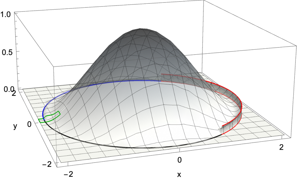
Figure 1: Left: Cartoon-like function with jump discontinuities in the zeroth (red), first (blue) and second (black) order directional derivative on a circle with radius 2 2
For all 𝐱 ∈ ∂ T \mathbf{x}\in\partial T 𝐧 ( 𝐱 ) = ( cos ( ϑ 𝐱 ) , sin ( ϑ 𝐱 ) ) T , ϑ 𝐱 ∈ [ 0 , 2 π ) , \mathbf{n}(\mathbf{x})=(\cos(\vartheta_{\mathbf{x}}),\sin(\vartheta_{\mathbf{x}}))^{\mathrm{T}},\,\vartheta_{\mathbf{x}}\in[0,2\pi), ∂ T \partial T 𝐱 \mathbf{x} 𝔣 ∈ ℰ u + 1 ( τ ) \mathfrak{f}\in\mathcal{E}^{u+1}(\tau) Definition 3.1 u > 4 u>4 2 π 2\pi 𝔣 2 π \mathfrak{f}^{2\pi} Ψ ( 𝔦 ) ∈ 𝒲 2 q \Psi^{(\mathfrak{i})}\in\mathcal{W}^{2q} 2 q ≥ u 2q\geq u 𝔦 ∈ { 𝔥 , 𝔳 } \mathfrak{i}\in\left\{\mathfrak{h},\mathfrak{v}\right\} Eq. 2 ψ j , ℓ , 𝐲 ( 𝔦 ) \psi_{j,\ell,\mathbf{y}}^{(\mathfrak{i})} Eq. 3
Theorem 3.1 .
Let j ∈ ℕ j\in\mathbb{N} ℓ ∈ ℤ \ell\in\mathbb{Z} | ℓ | < 2 j / 2 \left\lvert\ell\right\rvert<2^{j/2} 𝐲 ∈ 𝒫 ( 𝐍 j , ℓ ( 𝔦 ) ) \mathbf{y}\in\mathcal{P}(\mathbf{N}_{j,\ell}^{(\mathfrak{i})}) Q ∈ 𝒬 j 1 Q\in\mathcal{Q}_{j}^{1} 𝐱 0 : = 𝐱 0 ( Q ) ∈ ∂ T ∩ Q \mathbf{x}_{0}\mathrel{\mathop{:}}=\mathbf{x}_{0}(Q)\in\partial T\cap Q n : = n ( Q ) ∈ ℕ 0 n\mathrel{\mathop{:}}=n(Q)\in\mathbb{N}_{0} n < u n<u
∂ 𝚯 ( ϑ ) m [ f 1 ] ( 𝐱 ) = 0 and ∂ 𝚯 ( ϑ ) n [ f 1 ] ( 𝐱 ) ≠ 0 , \displaystyle\partial_{\boldsymbol{\Theta}(\vartheta)}^{m}[f_{1}](\mathbf{x})=0\quad\text{and}\quad\partial_{\boldsymbol{\Theta}(\vartheta)}^{n}[f_{1}](\mathbf{x})\neq 0, if 0 ≤ m < n , \displaystyle\quad\text{if }\,0\leq m<n,
f 1 ( 𝐱 ) ≠ 0 , \displaystyle f_{1}(\mathbf{x})\neq 0, if n = 0 , \displaystyle\quad\text{if }\,n=0,
is fulfilled for all 𝐱 ∈ ∂ T ∩ Q \mathbf{x}\in\partial T\cap Q ϑ ∈ ( θ j , ℓ − 2 ( 𝔦 ) , θ j , ℓ + 2 ( 𝔦 ) ) \vartheta\in\left(\theta_{j,\ell-2}^{(\mathfrak{i})},\theta_{j,\ell+2}^{(\mathfrak{i})}\right) C 1 > 0 C_{1}>0
| ⟨ 𝔣 2 π , ψ j , ℓ , 𝐲 ( 𝔦 ) ⟩ 2 | ≤ C 1 2 − 3 j / 4 ∑ Q ∈ 𝒬 j 1 ( 1 + 2 j / 2 | sin ( θ j , ℓ ( 𝔦 ) − ϑ 𝐱 0 ) | ) − 5 / 2 2 j n ( 1 + 2 j | 2 π 𝐲 − 𝐱 0 | 2 2 ) q , \left\lvert\left\langle\mathfrak{f}^{2\pi},\psi_{j,\ell,\mathbf{y}}^{(\mathfrak{i})}\right\rangle_{2}\right\rvert\leq C_{1}\,2^{-3j/4}\sum_{Q\in\mathcal{Q}_{j}^{1}}\frac{\left(1+2^{j/2}\left\lvert\sin(\theta_{j,\ell}^{(\mathfrak{i})}-\vartheta_{\mathbf{x}_{0}})\right\rvert\right)^{-5/2}}{2^{jn}\Bigl(1+2^{j}\left\lvert 2\pi\mathbf{y}-\mathbf{x}_{0}\right\rvert_{2}^{2}\Bigr)^{q}},
where C 1 = C 1 ( 𝔣 , Ψ ( 𝔦 ) , T ) C_{1}=C_{1}(\mathfrak{f},\Psi^{(\mathfrak{i})},T) j , ℓ j,\ell 𝐲 \mathbf{y}
For ε > 0 \varepsilon>0 T ∈ STAR 2 ( τ ) T\in\mathrm{STAR}^{2}(\tau) 𝐲 ∈ 𝒫 ( 𝐍 j , ℓ ( 𝔦 ) ) \mathbf{y}\in\mathcal{P}(\mathbf{N}_{j,\ell}^{(\mathfrak{i})})
U ε ( 𝐲 ) : = U ε , T ( 𝐲 ) : = ∂ T ∩ B ε ( 2 π 𝐲 ) . U_{\varepsilon}(\mathbf{y})\mathrel{\mathop{:}}=U_{\varepsilon,T}(\mathbf{y})\mathrel{\mathop{:}}=\partial T\cap B_{\varepsilon}(2\pi\mathbf{y}). (15)
Theorem 3.2 .
Let 0 < ε 0 ≤ 1 0<\varepsilon_{0}\leq 1 j ∈ ℕ j\in\mathbb{N} ℓ ∈ ℤ \ell\in\mathbb{Z} | ℓ | < 2 j / 2 \left\lvert\ell\right\rvert<2^{j/2} 𝐲 ∈ 𝒫 ( 𝐍 j , ℓ ( 𝔦 ) ) \mathbf{y}\in\mathcal{P}(\mathbf{N}_{j,\ell}^{(\mathfrak{i})})
i)
For ε = ε 0 2 − j / 2 \varepsilon=\varepsilon_{0}\,2^{-j/2} there exists 𝐱 0 ∈ U ε ( 𝐲 ) \mathbf{x}_{0}\in U_{\varepsilon}(\mathbf{y}) with ϑ 𝐱 0 ∈ ( θ j , ℓ − 2 ( 𝔦 ) , θ j , ℓ + 2 ( 𝔦 ) ) \vartheta_{\mathbf{x}_{0}}\in\left(\theta_{j,\ell-2}^{(\mathfrak{i})},\theta_{j,\ell+2}^{(\mathfrak{i})}\right) .
ii)
For n ∈ ℕ 0 n\in\mathbb{N}_{0} with 4 ( n + 1 ) < u 4(n+1)<u we have
∂ 𝚯 ( ϑ ) m [ f 1 ] ( 𝐱 ) = 0 and ∂ 𝚯 ( ϑ ) n [ f 1 ] ( 𝐱 ) ≠ 0 , \displaystyle\partial_{\boldsymbol{\Theta}(\vartheta)}^{m}[f_{1}](\mathbf{x})=0\quad\text{and}\quad\partial_{\boldsymbol{\Theta}(\vartheta)}^{n}[f_{1}](\mathbf{x})\neq 0, if 0 ≤ m < n , \displaystyle\quad\text{if }\,0\leq m<n, (16)
f 1 ( 𝐱 ) ≠ 0 , \displaystyle f_{1}(\mathbf{x})\neq 0, if n = 0 , \displaystyle\quad\text{if }\,n=0,
for all 𝐱 ∈ U ε ( 𝐲 ) \mathbf{x}\in U_{\varepsilon}(\mathbf{y}) and all ϑ ∈ ( θ j , ℓ − 2 ( 𝔦 ) , θ j , ℓ + 2 ( 𝔦 ) ) \vartheta\in\left(\theta_{j,\ell-2}^{(\mathfrak{i})},\theta_{j,\ell+2}^{(\mathfrak{i})}\right) .
Then there exists a constant C 2 > 0 C_{2}>0
| ⟨ 𝔣 2 π , ψ j , ℓ , 𝐲 ( 𝔦 ) ⟩ 2 | ≥ C 2 2 − j ( 3 / 4 + n ) , \left\lvert\left\langle\mathfrak{f}^{2\pi},\psi_{j,\ell,\mathbf{y}}^{(\mathfrak{i})}\right\rangle_{2}\right\rvert\geq C_{2}\,2^{-j(3/4+n)},
where C 2 = C 2 ( 𝔣 , Ψ ( 𝔦 ) , T , ε 0 ) C_{2}=C_{2}(\mathfrak{f},\Psi^{(\mathfrak{i})},T,\varepsilon_{0}) j , ℓ j,\ell 𝐲 \mathbf{y}
Figure 2: Left: Schematic visualization of the function from Fig. 1 ℒ ℓ ( 𝔦 ) , max \mathcal{L}^{(\mathfrak{i}),\mathrm{max}}_{\ell} ℒ ℓ ( 𝔦 ) , min \mathcal{L}^{(\mathfrak{i}),\mathrm{min}}_{\ell} Eq. 17 θ 10 , ℓ ( 𝔦 ) \theta_{10,\ell}^{(\mathfrak{i})}
At the end of this section, we include a small numerical example to visualize the main results. We construct a cartoon-like function 𝔣 \mathfrak{f} 2 2 Fig. 1 ( 2 cos θ , 2 sin θ ) T (2\cos\theta,\,2\sin\theta)^{\mathrm{T}} θ ∈ { π 3 , π , 5 π 3 } \theta\in\left\{\frac{\pi}{3},\pi,\frac{5\pi}{3}\right\} Fig. 2 j = 10 j=10 ε 0 = 1 2 \varepsilon_{0}=\frac{1}{2} ε = 1 2 2 − 5 = 1 64 \varepsilon=\frac{1}{2}\,2^{-5}=\frac{1}{64} 𝐌 10 = 2 10 𝐈 2 \mathbf{M}_{10}=2^{10}\,\mathbf{I}_{2} 𝐈 2 \mathbf{I}_{2} 𝐲 ∈ 𝒫 ( 𝐌 10 ) \mathbf{y}\in\mathcal{P}(\mathbf{M}_{10}) 𝐱 0 ∈ U ε ( 𝐲 ) \mathbf{x}_{0}\in U_{\varepsilon}(\mathbf{y}) ϑ 𝐱 0 ∈ ( θ 10 , ℓ − 2 ( 𝔦 ) , θ 10 , ℓ + 2 ( 𝔦 ) ) \vartheta_{\mathbf{x}_{0}}\in\left(\theta_{10,\ell-2}^{(\mathfrak{i})},\theta_{10,\ell+2}^{(\mathfrak{i})}\right) 𝒴 ℓ ( 𝔦 ) \mathcal{Y}_{\ell}^{(\mathfrak{i})} ℓ ∈ ℤ \ell\in\mathbb{Z} | ℓ | < 32 \left\lvert\ell\right\rvert<32 𝔦 ∈ { 𝔥 , 𝔳 } \mathfrak{i}\in\left\{\mathfrak{h},\mathfrak{v}\right\}
ℒ ℓ ( 𝔦 ) , max : = max 𝐲 ∈ 𝒴 ℓ ( 𝔦 ) | ⟨ 𝔣 2 π , ψ j , ℓ , 𝐲 ( 𝔦 ) ⟩ 2 | , ℒ ℓ ( 𝔦 ) , min : = min 𝐲 ∈ 𝒴 ℓ ( 𝔦 ) | ⟨ 𝔣 2 π , ψ j , ℓ , 𝐲 ( 𝔦 ) ⟩ 2 | \mathcal{L}^{(\mathfrak{i}),\mathrm{max}}_{\ell}\mathrel{\mathop{:}}=\max\limits_{\mathbf{y}\in\mathcal{Y}_{\ell}^{(\mathfrak{i})}}\left\lvert\left\langle\mathfrak{f}^{2\pi},\psi_{j,\ell,\mathbf{y}}^{(\mathfrak{i})}\right\rangle_{2}\right\rvert,\quad\mathcal{L}^{(\mathfrak{i}),\mathrm{min}}_{\ell}\mathrel{\mathop{:}}=\min\limits_{\mathbf{y}\in\mathcal{Y}_{\ell}^{(\mathfrak{i})}}\left\lvert\left\langle\mathfrak{f}^{2\pi},\psi_{j,\ell,\mathbf{y}}^{(\mathfrak{i})}\right\rangle_{2}\right\rvert (17)
and present them in the right picture of Fig. 2 θ 10 , ℓ ( 𝔦 ) \theta_{10,\ell}^{(\mathfrak{i})} | ⟨ 𝔣 2 π , ψ j , ℓ , 𝐲 ( 𝔦 ) ⟩ 2 | \left\lvert\left\langle\mathfrak{f}^{2\pi},\psi_{j,\ell,\mathbf{y}}^{(\mathfrak{i})}\right\rangle_{2}\right\rvert 𝔣 2 π \mathfrak{f}^{2\pi}
4 Proof of Theorem 3.1
The Fourier coefficients of a function f ∈ L 1 ( 𝕋 2 ) f\in L_{1}(\mathbb{T}^{2})
c 𝐤 ( f ) : = ( 2 π ) − 2 ∫ 𝕋 2 f ( 𝐱 ) e − i 𝐤 T 𝐱 𝑑 𝐱 , 𝐤 ∈ ℤ 2 c_{\mathbf{k}}(f)\mathrel{\mathop{:}}=(2\pi)^{-2}\int_{\mathbb{T}^{2}}f(\mathbf{x})\,\mathrm{e}^{-\mathrm{i}\mathbf{k}^{\mathrm{T}}\mathbf{x}}\,\mathrm{d}\mathbf{x},\qquad\mathbf{k}\in\mathbb{Z}^{2}
and the Fourier transform of f ∈ L 1 ( ℝ 2 ) f\in L_{1}(\mathbb{R}^{2})
ℱ [ f ] ( 𝐱 ) : = ℱ f ( 𝐱 ) : = ( 2 π ) − 2 ∫ ℝ 2 f ( 𝝃 ) e − i 𝝃 T 𝐱 𝑑 𝝃 , 𝐱 ∈ ℝ 2 , \mathcal{F}[f](\mathbf{x})\mathrel{\mathop{:}}=\mathcal{F}f(\mathbf{x})\mathrel{\mathop{:}}=(2\pi)^{-2}\int_{\mathbb{R}^{2}}f(\boldsymbol{\xi})\,\mathrm{e}^{-\mathrm{i}\boldsymbol{\xi}^{\mathrm{T}}\mathbf{x}}\,\mathrm{d}\boldsymbol{\xi},\qquad\mathbf{x}\in\mathbb{R}^{2},
and we have the operator
ℱ − 1 [ f ] ( 𝐱 ) : = ℱ − 1 f ( 𝐱 ) : = ∫ ℝ 2 f ( 𝝃 ) e i 𝝃 T 𝐱 𝑑 𝝃 , 𝐱 ∈ ℝ 2 . \mathcal{F}^{-1}[f](\mathbf{x})\mathrel{\mathop{:}}=\mathcal{F}^{-1}f(\mathbf{x})\mathrel{\mathop{:}}=\int_{\mathbb{R}^{2}}f(\boldsymbol{\xi})\,\mathrm{e}^{\mathrm{i}\boldsymbol{\xi}^{\mathrm{T}}\mathbf{x}}\,\mathrm{d}\boldsymbol{\xi},\qquad\mathbf{x}\in\mathbb{R}^{2}.
Let q ∈ ℕ 0 q\in\mathbb{N}_{0} 𝐫 ∈ ℕ 0 2 \mathbf{r}\in\mathbb{N}_{0}^{2} | 𝐫 | 1 ≤ q \left\lvert\mathbf{r}\right\rvert_{1}\leq q f ∈ L 1 ( ℝ 2 ) f\in L_{1}(\mathbb{R}^{2}) ( i ∘ ) q f ∈ L 1 ( ℝ 2 ) (\mathrm{i}\,\circ)^{q}\,f\in L_{1}(\mathbb{R}^{2}) ℱ f ∈ C q ( ℝ 2 ) \mathcal{F}f\in C^{q}(\mathbb{R}^{2})
∂ 𝐫 ℱ f ( 𝝃 ) = ℱ [ ( i ∘ ) 𝐫 f ( 𝐱 ) ] ( 𝝃 ) . \partial^{\mathbf{r}}\mathcal{F}f(\boldsymbol{\xi})=\mathcal{F}\left[(\mathrm{i}\,\circ)^{\mathbf{r}}\,f(\mathbf{x})\right](\boldsymbol{\xi}). (18)
For f ∈ C q ( ℝ 2 ) f\in C^{q}(\mathbb{R}^{2}) ∂ 𝐫 f ∈ L 1 ( ℝ 2 ) \partial^{\mathbf{r}}f\in L_{1}(\mathbb{R}^{2})
ℱ [ ∂ 𝐫 f ] ( 𝝃 ) = ( i 𝝃 ) 𝐫 ℱ f ( 𝝃 ) \mathcal{F}\left[\partial^{\mathbf{r}}f\right](\boldsymbol{\xi})=(\mathrm{i}\,\boldsymbol{\xi})^{\mathbf{r}}\,\mathcal{F}f(\boldsymbol{\xi}) (19)
and from Eq. 12 Eq. 19 m m 𝐯 ∈ ℝ 2 \mathbf{v}\in\mathbb{R}^{2}
ℱ [ ∂ 𝐯 m f ] ( 𝝃 ) = ∑ | 𝐫 | 1 = m ( m 𝐫 ) 𝐯 𝐫 ℱ [ ∂ 𝐫 f ] ( 𝝃 ) = i m ℱ f ( 𝝃 ) ∑ | 𝐫 | 1 = m ( m 𝐫 ) 𝐯 𝐫 𝝃 𝐫 = i m ( 𝐯 T 𝝃 ) m ℱ f ( 𝝃 ) . \mathcal{F}\left[\partial^{m}_{\mathbf{v}}f\right](\boldsymbol{\xi})=\sum_{\left\lvert\mathbf{r}\right\rvert_{1}=m}\binom{m}{\mathbf{r}}\mathbf{v}^{\mathbf{r}}\mathcal{F}\left[\partial^{\mathbf{r}}f\right](\boldsymbol{\xi})=\mathrm{i}^{m}\mathcal{F}f(\boldsymbol{\xi})\sum_{\left\lvert\mathbf{r}\right\rvert_{1}=m}\binom{m}{\mathbf{r}}\mathbf{v}^{\mathbf{r}}\boldsymbol{\xi}^{\mathbf{r}}=\mathrm{i}^{m}(\mathbf{v}^{\mathrm{T}}\boldsymbol{\xi})^{m}\mathcal{F}f(\boldsymbol{\xi}). (20)
For the remainder of this section we fix the function ϕ ∈ C 0 ∞ ( ℝ 2 ) \phi\in C_{0}^{\infty}\left(\mathbb{R}^{2}\right) supp ϕ ⊂ ( − π , π ) 2 \mathrm{supp}\,\phi\subset(-\pi,\pi)^{2} ϕ j : = ϕ ( 2 j / 2 ∘ ) \phi_{j}\mathrel{\mathop{:}}=\phi\left(2^{j/2}\circ\right) [2 , Chapter 6.1] , we assume that for sufficiently large j ≥ j 0 j\geq j_{0} ∂ T \partial T ϕ Q , Q ∈ 𝒬 j 1 , \phi_{Q},\,Q\in\mathcal{Q}_{j}^{1},\, ( x 1 , E ( x 1 ) ) T (x_{1},E(x_{1}))^{\mathrm{T}} ( E ( x 2 ) , x 2 ) T (E(x_{2}),x_{2})^{\mathrm{T}}
Definition 4.1 .
For x 2 ∈ [ − 2 − j / 2 , 2 − j / 2 ] x_{2}\in\left[-2^{-j/2},2^{-j/2}\right] ( E ( x 2 ) , x 2 ) T (E(x_{2}),x_{2})^{\mathrm{T}} ∂ T \partial T E ( 0 ) = E ′ ( 0 ) = 0 E(0)=E^{\prime}(0)=0 f ∈ C 2 ( ℝ 2 ) f\in C^{2}(\mathbb{R}^{2})
𝒦 j ( 𝐱 ) = f ( 𝐱 ) ϕ j ( 𝐱 ) χ { 𝐱 : x 1 ≥ t ( x 2 ) } ( 𝐱 ) \mathcal{K}_{j}(\mathbf{x})=f(\mathbf{x})\,\phi_{j}(\mathbf{x})\,\chi_{\{\mathbf{x}\,:\,x_{1}\geq t(x_{2})\}}(\mathbf{x})
standard edge fragment.
Let 𝒦 j , 𝐱 0 , ϑ \mathcal{K}_{j,\mathbf{x}_{0},\vartheta} 𝐱 0 ∈ ∂ T \mathbf{x}_{0}\in\partial T 𝚯 ( ϑ ) = ( cos ϑ , sin ϑ ) T \boldsymbol{\Theta}(\vartheta)=(\cos{\vartheta},\sin{\vartheta})^{\mathrm{T}} ϑ ∈ [ 0 , 2 π ) \vartheta\in[0,2\pi) 𝒦 j , 𝟎 , 0 = 𝒦 j \mathcal{K}_{j,\mathbf{0},0}=\mathcal{K}_{j} [2 , Corollary 6.7] that the corresponding Fourier transform fulfills
ℱ 𝒦 j , 𝐱 0 , ϑ ( 𝝃 ) = e − i 𝐱 0 T 𝝃 ℱ 𝒦 j ( 𝐑 ϑ T 𝝃 ) , \mathcal{F}\mathcal{K}_{j,\mathbf{x}_{0},\vartheta}(\boldsymbol{\xi})=\mathrm{e}^{-\mathrm{i}\,\mathbf{x}_{0}^{\mathrm{T}}\boldsymbol{\xi}}\,\mathcal{F}\mathcal{K}_{j}(\mathbf{R}_{\vartheta}^{\mathrm{T}}\,\boldsymbol{\xi}), (21)
where 𝐑 ϑ \mathbf{R}_{\vartheta} ϑ \vartheta [22 , Lemma 6] .
Lemma 4.1 .
For 𝔦 ∈ { 𝔥 , 𝔳 } \mathfrak{i}\in\{\mathfrak{h},\mathfrak{v}\} q ∈ ℕ 0 q\in\mathbb{N}_{0} Ψ ( 𝔦 ) ∈ 𝒲 q \Psi^{(\mathfrak{i})}\in\mathcal{W}^{q} 𝒦 j , 𝟎 , ϑ \mathcal{K}_{j,\mathbf{0},\vartheta} ϑ ∈ ( θ j , ℓ − 2 ( 𝔦 ) , θ j , ℓ + 2 ( 𝔦 ) ) \vartheta\in\left(\theta_{j,\ell-2}^{(\mathfrak{i})},\theta_{j,\ell+2}^{(\mathfrak{i})}\right) f j = f ϕ j f_{j}=f\,\phi_{j} ∂ 𝚯 ( θ j , ℓ ( 𝔦 ) ) n f j = 𝒦 j , 𝟎 , ϑ \partial_{\boldsymbol{\Theta}(\theta_{j,\ell}^{(\mathfrak{i})})}^{n}f_{j}=\mathcal{K}_{j,\mathbf{0},\vartheta} n ∈ ℕ 0 n\in\mathbb{N}_{0} 𝐫 ∈ ℕ 0 2 \mathbf{r}\in\mathbb{N}_{0}^{2}
‖ ∂ 𝐫 [ ℱ [ f j ] Ψ j , ℓ ( 𝔦 ) ] ‖ supp Ψ j , ℓ ( 𝔦 ) , 2 2 ≤ C ( n , 𝐫 ) 2 − j ( 3 / 2 + 2 n + | 𝐫 | 1 ) ( 1 + 2 j / 2 | sin ( θ j , ℓ ( 𝔦 ) − ϑ ) | ) − 5 . \left\lVert\partial^{\mathbf{r}}\left[\mathcal{F}\left[f_{j}\right]\,\Psi_{j,\ell}^{(\mathfrak{i})}\right]\right\rVert^{2}_{\mathrm{supp}\,\Psi_{j,\ell}^{(\mathfrak{i})},2}\leq C(n,\mathbf{r})\,2^{-j(3/2+2n+\left\lvert\mathbf{r}\right\rvert_{1})}\,\left(1+2^{j/2}\left\lvert\sin(\theta_{j,\ell}^{(\mathfrak{i})}-\vartheta)\right\rvert\right)^{-5}.
Proof.
We use an idea from [2 , Corollary 6.6] and define ϕ 𝐫 ( 𝐱 ) : = 𝐱 𝐫 ϕ ( 𝐱 ) \phi_{\mathbf{r}}(\mathbf{x})\mathrel{\mathop{:}}=\mathbf{x}^{\mathbf{r}}\,\phi(\mathbf{x}) ϕ 𝐫 ( 2 j / 2 ∘ ) ∈ C 0 ∞ ( ℝ 2 ) \phi_{\mathbf{r}}\left(2^{j/2}\circ\right)\in C^{\infty}_{0}\left(\mathbb{R}^{2}\right) | supp ϕ 𝐫 ( 2 j / 2 ∘ ) | ≤ 2 − j \left\lvert\mathrm{supp}\,\phi_{\mathbf{r}}\left(2^{j/2}\circ\right)\right\rvert\leq 2^{-j}
𝐱 𝐫 f j ( 𝐱 ) = 2 − j | 𝐫 | 1 / 2 f ( 𝐱 ) ϕ 𝐫 ( 2 j / 2 𝐱 ) = 2 − j | 𝐫 1 | / 2 f j , 𝐫 ( 𝐱 ) , \mathbf{x}^{\mathbf{r}}f_{j}(\mathbf{x})=2^{-j\left\lvert\mathbf{r}\right\rvert_{1}/2}\,f(\mathbf{x})\,\phi_{\mathbf{r}}\left(2^{j/2}\,\mathbf{x}\right)=2^{-j\left\lvert\mathbf{r}_{1}\right\rvert/2}f_{j,\mathbf{r}}(\mathbf{x}),
where f j , 𝐫 : = f ϕ 𝐫 ( 2 j / 2 ∘ ) f_{j,\mathbf{r}}\mathrel{\mathop{:}}=f\,\phi_{\mathbf{r}}\left(2^{j/2}\,\circ\right) f j , 𝐫 f_{j,\mathbf{r}} ∂ 𝜽 ( θ j , ℓ ( 𝔦 ) ) n f j , 𝐫 = 𝒦 j , 𝟎 , ϑ \partial_{\boldsymbol{\theta}(\theta_{j,\ell}^{(\mathfrak{i})})}^{n}f_{j,\mathbf{r}}=\mathcal{K}_{j,\mathbf{0},\vartheta} Eq. 18
∂ 𝐫 ℱ f j ( 𝝃 ) = ℱ [ ( i ∘ ) 𝐫 f j ( ∘ ) ] ( 𝝃 ) = i 𝐫 2 − j | 𝐫 | 1 / 2 ℱ [ f ( ∘ ) ϕ 𝐫 ( 2 j / 2 ∘ ) ] ( 𝝃 ) \partial^{\mathbf{r}}\mathcal{F}f_{j}(\boldsymbol{\xi})=\mathcal{F}\left[(\mathrm{i}\,\circ)^{\mathbf{r}}f_{j}(\circ)\right](\boldsymbol{\xi})=\mathrm{i}^{\mathbf{r}}\,2^{-j\left\lvert\mathbf{r}\right\rvert_{1}/2}\,\mathcal{F}\left[f(\circ)\,\phi_{\mathbf{r}}\left(2^{j/2}\circ\right)\right](\boldsymbol{\xi}) (22)
and with Eq. 22 Eq. 20
∫ supp Ψ j , ℓ ( 𝔦 ) | ∂ 𝐫 [ ℱ f j ] ( 𝝃 ) | 2 d 𝝃 \displaystyle\int\limits_{\mathrm{supp}\Psi_{j,\ell}^{(\mathfrak{i})}}\bigl\lvert\partial^{\mathbf{r}}\left[\mathcal{F}f_{j}\right](\boldsymbol{\xi})\bigr\rvert^{2}\mathrm{d}\boldsymbol{\xi} = 2 − j | 𝐫 | 1 ∫ supp Ψ j , ℓ ( 𝔦 ) | ℱ f j , 𝐫 ( 𝝃 ) | 2 d 𝝃 \displaystyle=2^{-j\left\lvert\mathbf{r}\right\rvert_{1}}\int\limits_{\mathrm{supp}\Psi_{j,\ell}^{(\mathfrak{i})}}\bigl\lvert\mathcal{F}f_{j,\mathbf{r}}(\boldsymbol{\xi})\bigr\rvert^{2}\mathrm{d}\boldsymbol{\xi}
= 2 − j | 𝐫 | 1 ∫ supp Ψ j , ℓ ( 𝔦 ) | ( 𝚯 T ( θ j , ℓ ( 𝔦 ) ) 𝝃 ) − n ℱ [ 𝒦 j , 𝟎 , ϑ ] ( 𝝃 ) | 2 𝑑 𝝃 . \displaystyle=2^{-j\left\lvert\mathbf{r}\right\rvert_{1}}\int\limits_{\mathrm{supp}\Psi_{j,\ell}^{(\mathfrak{i})}}\left\lvert\left(\boldsymbol{\Theta}^{\mathrm{T}}(\theta_{j,\ell}^{(\mathfrak{i})})\,\boldsymbol{\xi}\right)^{-n}\mathcal{F}[\mathcal{K}_{j,\mathbf{0},\vartheta}](\boldsymbol{\xi})\right\rvert^{2}\mathrm{d}\boldsymbol{\xi}. (23)
In the following, we need a result from [2 , Theorem 6.1] given by
∫ | ρ | ∈ I j | ℱ 𝒦 j ( ρ 𝚯 ( θ − ϑ ) ) | 2 𝑑 ρ ≤ C 2 − 2 j ( 1 + 2 j / 2 | sin ( θ − ϑ ) | ) − 5 , \int\limits_{\left\lvert\rho\right\rvert\in I_{j}}\left\lvert\mathcal{F}\mathcal{K}_{j}\Bigr(\rho\,\boldsymbol{\Theta}(\theta-\vartheta)\Bigl)\right\rvert^{2}\mathrm{d}\rho\leq C\,2^{-2j}\,\Bigl(1+2^{j/2}\left\lvert\sin\left(\theta-\vartheta\right)\right\rvert\Bigr)^{-5}, (24)
where I j = [ 2 j − 1 , 2 j + 1 ] I_{j}=\left[2^{j-1},2^{j+1}\right] 𝝃 = ρ 𝚯 ( θ ) \boldsymbol{\xi}=\rho\,\boldsymbol{\Theta}(\theta) ρ = | 𝝃 | 2 \rho=\left\lvert\boldsymbol{\xi}\right\rvert_{2} Eq. 23
| 𝚯 T ( θ j , ℓ ( 𝔦 ) ) 𝝃 | = | ρ cos ( θ j , ℓ ( 𝔦 ) − θ ) | ≥ C 2 | ρ | , \left\lvert\boldsymbol{\Theta}^{\mathrm{T}}(\theta_{j,\ell}^{(\mathfrak{i})})\,\boldsymbol{\xi}\right\rvert=\left\lvert\rho\,\cos\left(\theta_{j,\ell}^{(\mathfrak{i})}-\theta\right)\right\rvert\geq C_{2}\left\lvert\rho\right\rvert, (25)
if θ ∈ ( θ j , ℓ − 2 ( 𝔦 ) , θ j , ℓ + 2 ( 𝔦 ) ) \theta\in\left(\theta_{j,\ell-2}^{(\mathfrak{i})},\theta_{j,\ell+2}^{(\mathfrak{i})}\right)
( θ j , ℓ + 2 ( 𝔦 ) − θ j , ℓ − 2 ( 𝔦 ) ) ≤ C 3 2 − j / 2 . \Bigl(\theta_{j,\ell+2}^{(\mathfrak{i})}-\theta_{j,\ell-2}^{(\mathfrak{i})}\Bigr)\leq C_{3}\,2^{-j/2}. (26)
We transform the integral from Eq. 23 Eq. 24 Eq. 25 Eq. 26 [22 , Lemma 1] to finally get
∫ supp Ψ j , ℓ ( 𝔦 ) | ∂ 𝐫 [ ℱ f j ] ( 𝝃 ) | 2 d 𝝃 \displaystyle\int\limits_{\mathrm{supp}\Psi_{j,\ell}^{(\mathfrak{i})}}\bigl\lvert\partial^{\mathbf{r}}\left[\mathcal{F}f_{j}\right](\boldsymbol{\xi})\bigr\rvert^{2}\mathrm{d}\boldsymbol{\xi} = 2 − j | 𝐫 | 1 ∫ θ j , ℓ − 2 ( 𝔦 ) θ j , ℓ + 2 ( 𝔦 ) ∫ 2 j 3 2 j + 1 | ( ρ cos ( θ j , ℓ ( 𝔦 ) − θ ) ) − n ℱ 𝒦 j ( ρ 𝚯 ( θ − ϑ ) ) | 2 ρ 𝑑 ρ 𝑑 θ \displaystyle=2^{-j\left\lvert\mathbf{r}\right\rvert_{1}}\int\limits_{\theta_{j,\ell-2}^{(\mathfrak{i})}}^{\theta_{j,\ell+2}^{(\mathfrak{i})}}\int\limits_{\frac{2^{j}}{3}}^{2^{j+1}}\left\lvert\left(\rho\,\cos\left(\theta_{j,\ell}^{(\mathfrak{i})}-\theta\right)\right)^{-n}\mathcal{F}\mathcal{K}_{j}\Bigr(\rho\,\boldsymbol{\Theta}(\theta-\vartheta)\Bigl)\right\rvert^{2}\rho\,\mathrm{d}\rho\,\mathrm{d}\theta
≤ C 4 ( n , 𝐫 ) 2 − j ( 1 + 2 n + | 𝐫 | 1 ) ∫ θ j , ℓ − 2 ( 𝔦 ) θ j , ℓ + 2 ( 𝔦 ) ( 1 + 2 j / 2 | sin ( θ − ϑ ) | ) − 5 d θ \displaystyle\leq C_{4}(n,\mathbf{r})\,2^{-j(1+2n+\left\lvert\mathbf{r}\right\rvert_{1})}\int\limits_{\theta_{j,\ell-2}^{(\mathfrak{i})}}^{\theta_{j,\ell+2}^{(\mathfrak{i})}}\left(1+2^{j/2}\bigl\lvert\sin(\theta-\vartheta)\bigr\rvert\right)^{-5}\mathrm{d}\theta
≤ C 5 ( n , 𝐫 ) 2 − j ( 3 / 2 + 2 n + | 𝐫 | 1 ) ( 1 + 2 j / 2 | sin ( θ j , ℓ ( 𝔦 ) − ϑ ) | ) − 5 . \displaystyle\leq C_{5}(n,\mathbf{r})\,2^{-j(3/2+2n+\left\lvert\mathbf{r}\right\rvert_{1})}\left(1+2^{j/2}\left\lvert\sin(\theta_{j,\ell}^{(\mathfrak{i})}-\vartheta)\right\rvert\right)^{-5}. (27)
To obtain the desired estimate, we repeat the steps from the proof of [22 , Lemma 4] and apply Eq. 27
In the following, we consider the second order differential operator L : = I + 2 j Δ L\mathrel{\mathop{:}}=I+2^{j}\Delta [2 , 15 , 22 ] where Δ : = ∂ ( 2 , 0 ) + ∂ ( 0 , 2 ) \Delta\mathrel{\mathop{:}}=\partial^{(2,0)}+\partial^{(0,2)} [22 , Lemma 8] . The proof is similar and will be omitted.
Lemma 4.2 .
For 𝔦 ∈ { 𝔥 , 𝔳 } \mathfrak{i}\in\{\mathfrak{h},\mathfrak{v}\} q ∈ ℕ 0 q\in\mathbb{N}_{0} Ψ ( 𝔦 ) ∈ 𝒲 2 q \Psi^{(\mathfrak{i})}\in\mathcal{W}^{2q} f j , 0 : = f 0 ϕ j f_{j,0}\mathrel{\mathop{:}}=f_{0}\,\phi_{j} f 0 ∈ C 0 u ( ℝ 2 ) f_{0}\in C_{0}^{u}\left(\mathbb{R}^{2}\right) u ∈ ℕ 0 u\in\mathbb{N}_{0} 𝒦 j , 𝟎 , ϑ \mathcal{K}_{j,\mathbf{0},\vartheta} ϑ ∈ ( θ j , ℓ − 2 ( 𝔦 ) , θ j , ℓ + 2 ( 𝔦 ) ) \vartheta\in\left(\theta_{j,\ell-2}^{(\mathfrak{i})},\theta_{j,\ell+2}^{(\mathfrak{i})}\right) f j , 1 : = f 1 ϕ j f_{j,1}\mathrel{\mathop{:}}=f_{1}\,\phi_{j} ∂ 𝚯 ( θ j , ℓ ( 𝔦 ) ) n f j , 1 = 𝒦 j , 𝟎 , ϑ \partial_{\boldsymbol{\Theta}(\theta_{j,\ell}^{(\mathfrak{i})})}^{n}f_{j,1}=\mathcal{K}_{j,\mathbf{0},\vartheta} n ∈ ℕ 0 n\in\mathbb{N}_{0} C 1 ( u , q ) , C 2 ( n , q ) > 0 C_{1}(u,q),C_{2}(n,q)>0
‖ L q [ ℱ [ h ] Ψ j , ℓ ( 𝔦 ) ] ‖ supp Ψ j , ℓ ( 𝔦 ) , 2 2 ≤ { C 1 ( u , q ) 2 − j ( 2 u + 1 ) , if h = f j , 0 , C 2 ( n , q ) 2 − j ( 3 / 2 + 2 n ) ( 1 + 2 j / 2 | sin ( θ j , ℓ ( 𝔦 ) − ϑ ) | ) 5 , if h = f j , 1 . \left\lVert L^{q}\left[\mathcal{F}[h]\,\Psi_{j,\ell}^{(\mathfrak{i})}\right]\right\rVert^{2}_{\mathrm{supp}\,\Psi_{j,\ell}^{(\mathfrak{i})},2}\leq\begin{cases}C_{1}(u,q)\,2^{-j(2u+1)},&\text{if }h=f_{j,0},\\
\dfrac{C_{2}(n,q)\,2^{-j(3/2+2n)}}{\left(1+2^{j/2}\left\lvert\sin\left(\theta_{j,\ell}^{(\mathfrak{i})}-\vartheta\right)\right\rvert\right)^{5}},&\text{if }h=f_{j,1}.\end{cases}
We are ready to prove the first main theorem of this paper.
Let T ∈ STAR 2 ( τ ) T\in\mathrm{STAR}^{2}(\tau) 𝔣 : = f χ T ∈ ℰ u + 1 ( τ ) \mathfrak{f}\mathrel{\mathop{:}}=f\,\chi_{T}\in\mathcal{E}^{u+1}(\tau) ϕ Q ∈ C 0 ∞ ( ℝ 2 ) , Q ∈ 𝒬 j , \phi_{Q}\in C_{0}^{\infty}\left(\mathbb{R}^{2}\right),\,Q\in\mathcal{Q}_{j}, Eq. 13 Eq. 14 𝔣 \mathfrak{f}
𝔣 = ∑ Q ∈ 𝒬 j 𝔣 Q = ∑ Q ∈ 𝒬 j 0 𝔣 Q + ∑ Q ∈ 𝒬 j 1 𝔣 Q , \mathfrak{f}=\sum_{Q\in\mathcal{Q}_{j}}\mathfrak{f}_{Q}=\sum_{Q\in\mathcal{Q}_{j}^{0}}\mathfrak{f}_{Q}+\sum_{Q\in\mathcal{Q}_{j}^{1}}\mathfrak{f}_{Q}, (28)
where 𝔣 Q : = 𝔣 ϕ Q \mathfrak{f}_{Q}\mathrel{\mathop{:}}=\mathfrak{f}\,\phi_{Q} [2 , Section 5.1] that there are constants C 1 , C 2 > 0 C_{1},C_{2}>0
| 𝒬 j 0 | ≤ C 1 2 j , | 𝒬 j 1 | ≤ C 2 2 j / 2 . \left\lvert\mathcal{Q}_{j}^{0}\right\rvert\leq C_{1}\,2^{j},\qquad\qquad\left\lvert\mathcal{Q}_{j}^{1}\right\rvert\leq C_{2}\,2^{j/2}. (29)
We denote by 𝔣 Q 2 π \mathfrak{f}_{Q}^{2\pi} 2 π 2\pi 𝔣 Q \mathfrak{f}_{Q} 𝔣 Q ∈ L 1 ( ℝ 2 ) \mathfrak{f}_{Q}\in L_{1}(\mathbb{R}^{2}) 𝔣 Q 2 π \mathfrak{f}_{Q}^{2\pi}
c 𝐤 ( 𝔣 Q 2 π ) = ℱ [ 𝔣 Q ] ( 𝐤 ) , 𝐤 ∈ ℤ 2 . c_{\mathbf{k}}(\mathfrak{f}_{Q}^{2\pi})=\mathcal{F}[\mathfrak{f}_{Q}](\mathbf{k}),\qquad\mathbf{k}\in\mathbb{Z}^{2}.
From Eq. 18 ℱ [ 𝔣 Q ] ∈ C 2 q ( ℝ 2 ) \mathcal{F}[\mathfrak{f}_{Q}]\in C^{2q}(\mathbb{R}^{2}) 𝔣 Q \mathfrak{f}_{Q} Ψ j , ℓ ( 𝔦 ) ∈ 𝒲 2 q \Psi_{j,\ell}^{(\mathfrak{i})}\in\mathcal{W}^{2q} 2 q > 4 2q>4 ℱ [ 𝔣 Q ] Ψ j , ℓ ( 𝔦 ) ∈ C 0 2 q ( ℝ 2 ) \mathcal{F}[\mathfrak{f}_{Q}]\,\Psi_{j,\ell}^{(\mathfrak{i})}\in C_{0}^{2q}(\mathbb{R}^{2}) [22 ] ) to obtain
⟨ 𝔣 Q 2 π , ψ j , ℓ , 𝐲 ( 𝔦 ) ⟩ 2 = 2 − 3 j / 4 ∑ 𝐤 ∈ ℤ 2 ℱ [ 𝔣 Q ] ( 𝐤 ) Ψ j , ℓ ( 𝔦 ) ( 𝐤 ) e 2 π i 𝐤 T 𝐲 = 2 − 3 j / 4 ∑ 𝐧 ∈ ℤ 2 S Q ( 𝐧 ) , \left\langle\mathfrak{f}_{Q}^{2\pi},\psi^{(\mathfrak{i})}_{j,\ell,\mathbf{y}}\right\rangle_{2}=2^{-3j/4}\sum_{\mathbf{k}\in\mathbb{Z}^{2}}\mathcal{F}[\mathfrak{f}_{Q}](\mathbf{k})\,\Psi^{(\mathfrak{i})}_{j,\ell}(\mathbf{k})\,\mathrm{e}^{2\pi\mathrm{i}\mathbf{k}^{\mathrm{T}}\mathbf{y}}=2^{-3j/4}\sum_{\mathbf{n}\in\mathbb{Z}^{2}}S_{Q}(\mathbf{n}), (30)
where
S Q ( 𝐧 ) : = ℱ − 1 [ ℱ [ 𝔣 Q ] Ψ j , ℓ ( 𝔦 ) ] ( 2 π ( 𝐲 + 𝐧 ) ) = ∫ ℝ 2 ℱ [ 𝔣 Q ] ( 𝝃 ) Ψ j , ℓ ( 𝔦 ) ( 𝝃 ) e 2 π i 𝝃 T ( 𝐲 + 𝐧 ) 𝑑 𝝃 . S_{Q}(\mathbf{n})\mathrel{\mathop{:}}=\mathcal{F}^{-1}\left[\mathcal{F}[\mathfrak{f}_{Q}]\Psi^{(\mathfrak{i})}_{j,\ell}\right]\Bigl(2\pi(\mathbf{y}+\mathbf{n})\Bigr)=\int\limits_{\mathbb{R}^{2}}\mathcal{F}[\mathfrak{f}_{Q}](\boldsymbol{\xi})\,\Psi^{(\mathfrak{i})}_{j,\ell}(\boldsymbol{\xi})\,\mathrm{e}^{2\pi\mathrm{i}\boldsymbol{\xi}^{\mathrm{T}}(\mathbf{y}+\mathbf{n})}\,\mathrm{d}\boldsymbol{\xi}.
We follow some of the steps in the proof of [22 , Theorem 3.1] and use repeated partial integration and Hölder’s inequality to obtain
| S Q ( 𝐧 ) | ≤ 2 3 j / 4 ( 1 + 2 j | 2 π ( 𝐲 + 𝐧 ) | 2 2 ) − q ‖ L q [ ℱ [ 𝔣 Q ] Ψ j , ℓ ( 𝔦 ) ] ‖ supp Ψ j , ℓ ( 𝔦 ) , 2 . \bigl\lvert S_{Q}(\mathbf{n})\bigr\rvert\leq 2^{3j/4}\Bigl(1+2^{j}\left\lvert 2\pi(\mathbf{y}+\mathbf{n})\right\rvert_{2}^{2}\Bigr)^{-q}\left\lVert L^{q}\left[\mathcal{F}[\mathfrak{f}_{Q}]\,\Psi^{(\mathfrak{i})}_{j,\ell}\right]\right\rVert_{\mathrm{supp}\,\Psi_{j,\ell}^{(\mathfrak{i})},2}. (31)
In [22 , Theorem 3.1] it was also shown that
∑ 𝐧 ∈ ℤ 2 ∖ { 𝟎 } ( 1 + 2 j | 2 π ( 𝐲 + 𝐧 ) | 2 2 ) − q ≤ C 2 ( q ) 2 − j q , \sum_{\mathbf{n}\in\mathbb{Z}^{2}\setminus\{\mathbf{0}\}}\Bigl(1+2^{j}\left\lvert 2\pi(\mathbf{y}+\mathbf{n})\right\rvert_{2}^{2}\Bigr)^{-q}\leq C_{2}(q)\,2^{-jq},
which leads to
2 − 3 j / 4 ∑ 𝐧 ∈ ℤ 2 ∖ { 𝟎 } | S Q ( 𝐧 ) | ≤ C ( q ) 2 − j q ‖ L q [ ℱ [ 𝔣 Q ] Ψ j , ℓ ( 𝔦 ) ] ‖ supp Ψ j , ℓ ( 𝔦 ) , 2 . 2^{-3j/4}\sum_{\mathbf{n}\in\mathbb{Z}^{2}\setminus\{\mathbf{0}\}}\bigl\lvert S_{Q}(\mathbf{n})\bigr\rvert\leq C(q)\,2^{-jq}\left\lVert L^{q}\left[\mathcal{F}[\mathfrak{f}_{Q}]\,\Psi^{(\mathfrak{i})}_{j,\ell}\right]\right\rVert_{\mathrm{supp}\,\Psi_{j,\ell}^{(\mathfrak{i})},2}. (32)
In the following, we distinguish wether the boundary ∂ T \partial T ϕ Q \phi_{Q}
i)
Let Q ∈ 𝒬 j 0 Q\in\mathcal{Q}_{j}^{0} Q ∩ T = ∅ Q\cap T=\emptyset 𝔣 Q = 0 \mathfrak{f}_{Q}=0
| ⟨ 𝔣 Q 2 π , ψ j , ℓ , 𝐲 ( 𝔦 ) ⟩ 2 | = 0 . \left\lvert\left\langle\mathfrak{f}_{Q}^{2\pi},\psi^{(\mathfrak{i})}_{j,\ell,\mathbf{y}}\right\rangle_{2}\right\rvert=0.
If Q ⊂ T Q\subset T 𝐱 1 ∈ [ − π , π ] 2 \mathbf{x}_{1}\in[-\pi,\pi]^{2}
| 2 π 𝐲 − 𝐱 1 | 2 ≥ C > 0 \left\lvert 2\pi\mathbf{y}-\mathbf{x}_{1}\right\rvert_{2}\geq C>0 (33)
and consider the function 𝔣 ~ Q ( 𝐱 ) : = 𝔣 Q ( 𝐱 + 𝐱 1 ) \widetilde{\mathfrak{f}}_{Q}(\mathbf{x})\mathrel{\mathop{:}}=\mathfrak{f}_{Q}(\mathbf{x}+\mathbf{x}_{1}) Eq. 21 ℱ [ 𝔣 Q ] ( 𝝃 ) = e − i 𝝃 T 𝐱 1 ℱ [ 𝔣 ~ Q ] ( 𝝃 ) \mathcal{F}[\mathfrak{f}_{Q}](\boldsymbol{\xi})=\mathrm{e}^{-\mathrm{i}\,\boldsymbol{\xi}^{\mathrm{T}}\mathbf{x}_{1}}\,\mathcal{F}[\widetilde{\mathfrak{f}}_{Q}](\boldsymbol{\xi})
S Q ( 𝟎 ) = ℱ − 1 [ ℱ [ 𝔣 Q ] Ψ j , ℓ ( 𝔦 ) ] ( 2 π 𝐲 ) = ∫ ℝ 2 ℱ [ 𝔣 ~ Q ] ( 𝝃 ) Ψ j , ℓ ( 𝔦 ) ( 𝝃 ) e i 𝝃 T ( 2 π 𝐲 − 𝐱 1 ) 𝑑 𝝃 . S_{Q}(\mathbf{0})=\mathcal{F}^{-1}\left[\mathcal{F}[\mathfrak{f}_{Q}]\Psi^{(\mathfrak{i})}_{j,\ell}\right](2\pi\mathbf{y})=\int\limits_{\mathbb{R}^{2}}\mathcal{F}[\widetilde{\mathfrak{f}}_{Q}](\boldsymbol{\xi})\,\Psi^{(\mathfrak{i})}_{j,\ell}(\boldsymbol{\xi})\,\mathrm{e}^{\mathrm{i}\,\boldsymbol{\xi}^{\mathrm{T}}(2\pi\mathbf{y}-\mathbf{x}_{1})}\,\mathrm{d}\boldsymbol{\xi}.
Since ℱ [ 𝔣 ~ Q ] Ψ j , ℓ ( 𝔦 ) ∈ C 0 q ( ℝ 2 ) \mathcal{F}[\widetilde{\mathfrak{f}}_{Q}]\,\Psi_{j,\ell}^{(\mathfrak{i})}\in C_{0}^{q}(\mathbb{R}^{2}) Eq. 31 Eq. 33
| S Q ( 𝟎 ) | ≤ 2 − j ( q − 3 / 4 ) ‖ L q [ ℱ [ 𝔣 ~ Q ] Ψ j , ℓ ( 𝔦 ) ] ‖ supp Ψ j , ℓ ( 𝔦 ) , 2 . \bigl\lvert S_{Q}(\mathbf{0})\bigr\rvert\leq 2^{-j(q-3/4)}\left\lVert L^{q}\left[\mathcal{F}[\widetilde{\mathfrak{f}}_{Q}]\,\Psi^{(\mathfrak{i})}_{j,\ell}\right]\right\rVert_{\mathrm{supp}\,\Psi_{j,\ell}^{(\mathfrak{i})},2}. (34)
Finally, the estimates Eq. 32 Eq. 34 Lemma 4.2 Eq. 30
| ⟨ 𝔣 Q 2 π , ψ j , ℓ , 𝐲 ( 𝔦 ) ⟩ 2 | ≤ 2 − 3 j / 4 ( | S Q ( 𝟎 ) | + ∑ 𝐧 ∈ ℤ 2 ∖ { 𝟎 } | S Q ( 𝐧 ) | ) ≤ C 1 ( u , q ) 2 − j ( q + u + 3 / 2 ) . \left\lvert\left\langle\mathfrak{f}_{Q}^{2\pi},\psi^{(\mathfrak{i})}_{j,\ell,\mathbf{y}}\right\rangle_{2}\right\rvert\leq 2^{-3j/4}\Bigl(\left\lvert S_{Q}(\mathbf{0})\right\rvert+\hskip-8.5359pt\sum_{\mathbf{n}\in\mathbb{Z}^{2}\setminus\{\mathbf{0}\}}\bigl\lvert S_{Q}(\mathbf{n})\bigr\rvert\Bigr)\leq C_{1}(u,q)\,2^{-j(q+u+3/2)}. (35)
ii)
Let Q ∈ 𝒬 j 1 Q\in\mathcal{Q}_{j}^{1}
S Q ( 𝟎 ) = ∫ ℝ 2 ℱ [ 𝔣 Q ] Ψ j , ℓ ( 𝔦 ) ( 𝝃 ) e i 𝝃 T ( 2 π 𝐲 − 𝐱 0 ) 𝑑 𝝃 , S_{Q}(\mathbf{0})=\int\limits_{\mathbb{R}^{2}}\mathcal{F}[\mathfrak{f}_{Q}]\,\Psi^{(\mathfrak{i})}_{j,\ell}(\boldsymbol{\xi})\,\mathrm{e}^{\mathrm{i}\,\boldsymbol{\xi}^{\mathrm{T}}(2\pi\mathbf{y}-\mathbf{x}_{0})}\,\mathrm{d}\boldsymbol{\xi},
where ∂ 𝚯 ( θ j , ℓ ( 𝔦 ) ) n 𝔣 Q = 𝒦 j , 𝟎 , ϑ 𝐱 0 \partial_{\boldsymbol{\Theta}(\theta_{j,\ell}^{(\mathfrak{i})})}^{n}\mathfrak{f}_{Q}=\mathcal{K}_{j,\mathbf{0},\vartheta_{\mathbf{x}_{0}}} 𝒦 j , 𝟎 , ϑ 𝐱 0 \mathcal{K}_{j,\mathbf{0},\vartheta_{\mathbf{x}_{0}}}
| S Q ( 𝟎 ) | ≤ 2 3 j / 4 ( 1 + 2 j | 2 π 𝐲 − 𝐱 0 | 2 2 ) − q ‖ L q [ ℱ [ f Q ] Ψ j , ℓ ( 𝔦 ) ] ‖ supp Ψ j , ℓ ( 𝔦 ) , 2 . \bigl\lvert S_{Q}(\mathbf{0})\bigr\rvert\leq 2^{3j/4}\Bigl(1+2^{j}\left\lvert 2\pi\mathbf{y}-\mathbf{x}_{0}\right\rvert_{2}^{2}\Bigr)^{-q}\left\lVert L^{q}\left[\mathcal{F}[f_{Q}]\,\Psi^{(\mathfrak{i})}_{j,\ell}\right]\right\rVert_{\mathrm{supp}\,\Psi_{j,\ell}^{(\mathfrak{i})},2}. (36)
From Eq. 32 Eq. 36 Lemma 4.2
| ⟨ 𝔣 Q 2 π , ψ j , ℓ , 𝐲 ( 𝔦 ) ⟩ 2 | \displaystyle\left\lvert\left\langle\mathfrak{f}_{Q}^{2\pi},\psi^{(\mathfrak{i})}_{j,\ell,\mathbf{y}}\right\rangle_{2}\right\rvert ≤ 2 − 3 j / 4 ( | S Q ( 𝟎 ) | + ∑ 𝐧 ∈ ℤ 2 ∖ { 𝟎 } | S Q ( 𝐧 ) | ) \displaystyle\leq 2^{-3j/4}\Bigl(\left\lvert S_{Q}(\mathbf{0})\right\rvert+\hskip-8.5359pt\sum_{\mathbf{n}\in\mathbb{Z}^{2}\setminus\{\mathbf{0}\}}\bigl\lvert S_{Q}(\mathbf{n})\bigr\rvert\Bigr)
≤ C 3 ( n , q ) 2 − 3 j / 4 ( 1 + 2 j / 2 | sin ( θ j , ℓ ( 𝔦 ) − ϑ 𝐱 0 ) | ) − 5 / 2 2 j n ( 1 + 2 j | 2 π 𝐲 − 𝐱 0 | 2 2 ) q . \displaystyle\leq C_{3}(n,q)\,2^{-3j/4}\frac{\left(1+2^{j/2}\left\lvert\sin(\theta_{j,\ell}^{(\mathfrak{i})}-\vartheta_{\mathbf{x}_{0}})\right\rvert\right)^{-5/2}}{2^{jn}\Bigl(1+2^{j}\left\lvert 2\pi\mathbf{y}-\mathbf{x}_{0}\right\rvert_{2}^{2}\Bigr)^{q}}. (37)
With the decomposition in Eq. 28 Eq. 35 ii)
| ⟨ 𝔣 2 π , ψ j , ℓ , 𝐲 ( 𝔦 ) ⟩ 2 | \displaystyle\left\lvert\left\langle\mathfrak{f}^{2\pi},\psi^{(\mathfrak{i})}_{j,\ell,\mathbf{y}}\right\rangle_{2}\right\rvert ≤ ∑ Q ∈ 𝒬 j 0 | ⟨ 𝔣 Q 2 π , ψ j , ℓ , 𝐲 ( 𝔦 ) ⟩ 2 | + ∑ Q ∈ 𝒬 j 1 | ⟨ 𝔣 Q 2 π , ψ j , ℓ , 𝐲 ( 𝔦 ) ⟩ 2 | \displaystyle\leq\sum_{Q\in\mathcal{Q}_{j}^{0}}\left\lvert\left\langle\mathfrak{f}_{Q}^{2\pi},\psi^{(\mathfrak{i})}_{j,\ell,\mathbf{y}}\right\rangle_{2}\right\rvert+\sum_{Q\in\mathcal{Q}_{j}^{1}}\left\lvert\left\langle\mathfrak{f}_{Q}^{2\pi},\psi^{(\mathfrak{i})}_{j,\ell,\mathbf{y}}\right\rangle_{2}\right\rvert
≤ C 4 ( u , n , q ) 2 − 3 j / 4 ∑ Q ∈ 𝒬 j 1 ( 1 + 2 j / 2 | sin ( θ j , ℓ ( 𝔦 ) − ϑ 𝐱 0 ) | ) − 5 / 2 2 j n ( 1 + 2 j | 2 π 𝐲 − 𝐱 0 | 2 2 ) q . \displaystyle\leq C_{4}(u,n,q)\,2^{-3j/4}\sum_{Q\in\mathcal{Q}_{j}^{1}}\frac{\left(1+2^{j/2}\left\lvert\sin(\theta_{j,\ell}^{(\mathfrak{i})}-\vartheta_{\mathbf{x}_{0}})\right\rvert\right)^{-5/2}}{2^{jn}\Bigl(1+2^{j}\left\lvert 2\pi\mathbf{y}-\mathbf{x}_{0}\right\rvert_{2}^{2}\Bigr)^{q}}. (38)
To finish the proof we consider general cartoon-like functions 𝔣 0 ∈ ℰ u + 1 ( τ ) \mathfrak{f}_{0}\in\mathcal{E}^{u+1}(\tau) 𝔣 0 = f 0 + f χ T = f 0 + 𝔣 \mathfrak{f}_{0}=f_{0}+f\,\chi_{T}=f_{0}+\mathfrak{f} 𝔣 = f χ T \mathfrak{f}=f\,\chi_{T} f 0 , f ∈ C 0 u + 1 ( ℝ 2 ) f_{0},f\in C_{0}^{u+1}\left(\mathbb{R}^{2}\right) T ∈ STAR 2 ( τ ) T\in\mathrm{STAR}^{2}(\tau) f 0 f_{0} f 0 , Q : = f 0 ϕ Q f_{0,Q}\mathrel{\mathop{:}}=f_{0}\,\phi_{Q}
f 0 = ∑ Q ∈ 𝒬 j 0 f 0 , Q , f_{0}=\sum_{Q\in\mathcal{Q}_{j}^{0}}f_{0,Q},
since 𝒬 j 1 = ∅ \mathcal{Q}_{j}^{1}=\emptyset Eq. 29 Eq. 35
| ⟨ f 0 2 π , ψ j , ℓ , 𝐲 ( 𝔦 ) ⟩ 2 | ≤ ∑ Q ∈ 𝒬 j 0 | ⟨ f 0 , Q 2 π , ψ j , ℓ , 𝐲 ( 𝔦 ) ⟩ 2 | ≤ C 5 ( u , q ) 2 − j ( q + u + 1 / 2 ) . \left\lvert\left\langle f_{0}^{2\pi},\psi^{(\mathfrak{i})}_{j,\ell,\mathbf{y}}\right\rangle_{2}\right\rvert\leq\sum_{Q\in\mathcal{Q}_{j}^{0}}\left\lvert\left\langle f_{0,Q}^{2\pi},\psi^{(\mathfrak{i})}_{j,\ell,\mathbf{y}}\right\rangle_{2}\right\rvert\leq C_{5}(u,q)\,2^{-j(q+u+1/2)}. (39)
The estimates ii) Eq. 39
| ⟨ 𝔣 0 2 π , ψ j , ℓ , 𝐲 ( 𝔦 ) ⟩ 2 | \displaystyle\left\lvert\left\langle\mathfrak{f}_{0}^{2\pi},\psi^{(\mathfrak{i})}_{j,\ell,\mathbf{y}}\right\rangle_{2}\right\rvert ≤ | ⟨ f 0 2 π , ψ j , ℓ , 𝐲 ( 𝔦 ) ⟩ 2 | + | ⟨ 𝔣 2 π , ψ j , ℓ , 𝐲 ( 𝔦 ) ⟩ 2 | \displaystyle\leq\left\lvert\left\langle f_{0}^{2\pi},\psi^{(\mathfrak{i})}_{j,\ell,\mathbf{y}}\right\rangle_{2}\right\rvert+\left\lvert\left\langle\mathfrak{f}^{2\pi},\psi^{(\mathfrak{i})}_{j,\ell,\mathbf{y}}\right\rangle_{2}\right\rvert
≤ C 6 ( u , n , q ) 2 − 3 j / 4 ∑ Q ∈ 𝒬 j 1 ( 1 + 2 j / 2 | sin ( θ j , ℓ ( 𝔦 ) − ϑ 𝐱 0 ) | ) − 5 / 2 2 j n ( 1 + 2 j | 2 π 𝐲 − 𝐱 0 | 2 2 ) q , \displaystyle\leq C_{6}(u,n,q)\,2^{-3j/4}\sum_{Q\in\mathcal{Q}_{j}^{1}}\frac{\left(1+2^{j/2}\left\lvert\sin(\theta_{j,\ell}^{(\mathfrak{i})}-\vartheta_{\mathbf{x}_{0}})\right\rvert\right)^{-5/2}}{2^{jn}\Bigl(1+2^{j}\left\lvert 2\pi\mathbf{y}-\mathbf{x}_{0}\right\rvert_{2}^{2}\Bigr)^{q}},
since n < u n<u
∎
5 Localization lemmata
Let T ∈ STAR 2 ( τ ) T\in\mathrm{STAR^{2}}(\tau) p : = p u : ℝ 2 → ℝ p\mathrel{\mathop{:}}=p_{u}:\mathbb{R}^{2}\rightarrow\mathbb{R} u u [12 , Lemma 4.1] the authors showed that the Fourier transform of the function P u : = p χ T P_{u}\mathrel{\mathop{:}}=p\,\chi_{T}
ℱ P u ( 𝝃 ) = ( 2 π ) − 2 ∫ T p ( 𝐱 ) e − i 𝝃 T 𝐱 𝑑 𝐱 = ∑ m = 0 u C m | 𝝃 | 2 m + 2 ∫ ∂ T p m ( 𝐱 , 𝝃 ) e − i 𝝃 T 𝐱 𝝃 T 𝐧 ( 𝐱 ) 𝑑 σ ( 𝐱 ) \mathcal{F}P_{u}(\boldsymbol{\xi})=(2\pi)^{-2}\int\limits_{T}p(\mathbf{x})\,\mathrm{e}^{-\mathrm{i}\boldsymbol{\xi}^{\mathrm{T}}\mathbf{x}}\,\mathrm{d}\mathbf{x}=\sum\limits_{m=0}^{u}\frac{C_{m}}{\left\lvert\boldsymbol{\xi}\right\rvert_{2}^{m+2}}\int\limits_{\partial T}p_{m}(\mathbf{x},\boldsymbol{\xi})\,\mathrm{e}^{-\mathrm{i}\boldsymbol{\xi}^{\mathrm{T}}\mathbf{x}}\,\boldsymbol{\xi}^{\mathrm{T}}\mathbf{n}(\mathbf{x})\,\mathrm{d}\sigma(\mathbf{x}) (40)
with constants C 0 , … , C u > 0 C_{0},\ldots,C_{u}>0 p 0 ( 𝐱 , 𝝃 ) : = p ( 𝐱 ) p_{0}(\mathbf{x},\boldsymbol{\xi})\mathrel{\mathop{:}}=p(\mathbf{x}) p m ( 𝐱 , 𝝃 ) : = 𝝃 T | 𝝃 | 2 grad 𝐱 [ p m − 1 ] ( 𝐱 , 𝝃 ) p_{m}(\mathbf{x},\boldsymbol{\xi})\mathrel{\mathop{:}}=\frac{\boldsymbol{\xi}^{\mathrm{T}}}{\left\lvert\boldsymbol{\xi}\right\rvert_{2}}\mathrm{grad}_{\mathbf{x}}[p_{m-1}](\mathbf{x},\boldsymbol{\xi}) ∂ T \partial T 𝐧 ( 𝐱 ) \mathbf{n}(\mathbf{x})
In the following lemma, we derive an explicit expression for the functions p m p_{m} Eq. 40
Lemma 5.1 .
Let T ∈ STAR 2 ( τ ) T\in\mathrm{STAR^{2}}(\tau) p = p u : ℝ 2 → ℝ p=p_{u}:\mathbb{R}^{2}\rightarrow\mathbb{R} u u C 0 , … , C u > 0 C_{0},\ldots,C_{u}>0 P u = p χ T P_{u}=p\,\chi_{T}
ℱ P u ( ρ 𝚯 ( θ ) ) = ∑ m = 0 u C m ρ m + 1 ∫ ∂ T ∂ 𝚯 ( θ ) m [ p ] ( 𝐱 ) e − i ρ 𝚯 T ( θ ) 𝐱 𝚯 T ( θ ) 𝐧 ( 𝐱 ) 𝑑 σ ( 𝐱 ) . \mathcal{F}P_{u}\left(\rho\,\boldsymbol{\Theta}(\theta)\right)=\sum\limits_{m=0}^{u}\frac{C_{m}}{\rho^{m+1}}\int\limits_{\partial T}\,\partial_{\boldsymbol{\Theta}(\theta)}^{m}[p](\mathbf{x})\,\mathrm{e}^{-\mathrm{i}\,\rho\,\boldsymbol{\Theta}^{\mathrm{T}}(\theta)\mathbf{x}}\,\boldsymbol{\Theta}^{\mathrm{T}}(\theta)\,\mathbf{n}(\mathbf{x})\,\mathrm{d}\sigma(\mathbf{x}). (41)
Proof.
By induction on the variable m m
p m ( 𝐱 , 𝝃 ) = | 𝝃 | 2 − m ∑ | 𝐫 | 1 = m ( m 𝐫 ) 𝝃 𝐫 ∂ 𝐫 [ p ] ( 𝐱 ) . p_{m}(\mathbf{x},\boldsymbol{\xi})=\left\lvert\boldsymbol{\xi}\right\rvert_{2}^{-m}\sum\limits_{\left\lvert\mathbf{r}\right\rvert_{1}=m}\binom{m}{\mathbf{r}}\,\boldsymbol{\xi}^{\mathbf{r}}\,\partial^{\mathbf{r}}[p](\mathbf{x}).
For m = 0 m=0 p 0 ( 𝐱 , 𝝃 ) = p p_{0}(\mathbf{x},\boldsymbol{\xi})=p m ∈ ℕ m\in\mathbb{N}
p m ( 𝐱 , 𝝃 ) = 𝝃 T | 𝝃 | 2 grad 𝐱 [ p m − 1 ] ( 𝐱 , 𝝃 ) = | 𝝃 | 2 − m ∑ | 𝐫 | 1 = m ( m 𝐫 ) 𝝃 𝐫 ∂ 𝐫 p . p_{m}(\mathbf{x},\boldsymbol{\xi})=\frac{\boldsymbol{\xi}^{\mathrm{T}}}{\left\lvert\boldsymbol{\xi}\right\rvert_{2}}\mathrm{grad}_{\mathbf{x}}[p_{m-1}](\mathbf{x},\boldsymbol{\xi})=\left\lvert\boldsymbol{\xi}\right\rvert_{2}^{-m}\sum\limits_{\left\lvert\mathbf{r}\right\rvert_{1}=m}\binom{m}{\mathbf{r}}\,\boldsymbol{\xi}^{\mathbf{r}}\,\partial^{\mathbf{r}}p.
It follows that
| 𝝃 | 2 m + 1 p m + 1 ( 𝐱 , 𝝃 ) \displaystyle\left\lvert\boldsymbol{\xi}\right\rvert_{2}^{m+1}p_{m+1}(\mathbf{x},\boldsymbol{\xi}) = 𝝃 T grad 𝐱 [ ∑ | 𝐫 | 1 = m ( m 𝐫 ) 𝝃 𝐫 ∂ 𝐫 p ] \displaystyle=\boldsymbol{\xi}^{\mathrm{T}}\mathrm{grad}_{\mathbf{x}}\left[\sum\limits_{\left\lvert\mathbf{r}\right\rvert_{1}=m}\binom{m}{\mathbf{r}}\boldsymbol{\xi}^{\mathbf{r}}\,\partial^{\mathbf{r}}p\right]
= ∑ r = 0 m ( m r ) ξ 1 r + 1 ξ 2 m − r ∂ ( r + 1 , 0 ) ∂ ( 0 , m − r ) p + ∑ r = 0 m ( m r ) ξ 1 r ξ 2 m − r + 1 ∂ ( r , 0 ) ∂ ( 0 , m − r + 1 ) p \displaystyle=\sum\limits_{r=0}^{m}\binom{m}{r}\,\xi_{1}^{r+1}\,\xi_{2}^{m-r}\,\partial^{(r+1,0)}\,\partial^{(0,m-r)}p+\sum\limits_{r=0}^{m}\binom{m}{r}\,\xi_{1}^{r}\,\xi_{2}^{m-r+1}\,\partial^{(r,0)}\,\partial^{(0,m-r+1)}p
= ∑ | 𝐫 | 1 = m + 1 ( m + 1 𝐫 ) 𝝃 𝐫 ∂ 𝐫 p . \displaystyle=\sum\limits_{\left\lvert\mathbf{r}\right\rvert_{1}=m+1}\binom{m+1}{\mathbf{r}}\,\boldsymbol{\xi}^{\mathbf{r}}\,\partial^{\mathbf{r}}p.
We use polar coordinates to verify
| 𝝃 | 2 − m 𝝃 𝐫 = ( cos θ ) r 1 ( sin θ ) r 2 = ( 𝚯 ( θ ) ) 𝐫 \left\lvert\boldsymbol{\xi}\right\rvert_{2}^{-m}\,\boldsymbol{\xi}^{\mathbf{r}}=(\cos\theta)^{r_{1}}\,(\sin\theta)^{r_{2}}=(\boldsymbol{\Theta}(\theta))^{\mathbf{r}}
if | 𝐫 | 1 = m \left\lvert\mathbf{r}\right\rvert_{1}=m Eq. 12
p m ( 𝐱 , ρ 𝚯 ( θ ) ) = ∑ | 𝐫 | 1 = m ( m 𝐫 ) ( 𝚯 ( θ ) ) 𝐫 ∂ 𝐫 [ p ] ( 𝐱 ) = ∂ 𝚯 ( θ ) m [ p ] ( 𝐱 ) . p_{m}(\mathbf{x},\rho\,\boldsymbol{\Theta}(\theta))=\sum\limits_{\left\lvert\mathbf{r}\right\rvert_{1}=m}\binom{m}{\mathbf{r}}\,(\boldsymbol{\Theta}(\theta))^{\mathbf{r}}\,\partial^{\mathbf{r}}[p](\mathbf{x})=\partial_{\boldsymbol{\Theta}(\theta)}^{m}[p](\mathbf{x}). (42)
We finish the proof by using polar coordinates for the variable 𝝃 \boldsymbol{\xi} Eq. 40 Eq. 42
Let 𝜸 : [ 0 , 2 π ) → ∂ T \boldsymbol{\gamma}:[0,2\pi)\rightarrow\partial T Eq. 11 M ∈ ℕ M\in\mathbb{N} a 0 < a 1 < … < a M a_{0}<a_{1}<\ldots<a_{M} [ 0 , 2 π ) [0,2\pi) x ∈ [ a k , a k + 1 ) , k = 0 , … , M − 1 , x\in[a_{k},a_{k+1}),k=0,\ldots,M-1, 𝜸 \boldsymbol{\gamma} ( x , f ( x ) ) T (x,f(x))^{\mathrm{T}} ( f ( x ) , x ) T (f(x),x)^{\mathrm{T}} 𝔦 = 𝔥 \mathfrak{i}=\mathfrak{h} ( f ( x ) , x ) T (f(x),x)^{\mathrm{T}} | f ′ ( x ) | ≤ 1 \left\lvert f^{\prime}(x)\right\rvert\leq 1 ( x , f ( x ) ) T (x,f(x))^{\mathrm{T}} | f ′ ( x ) | < 1 \left\lvert f^{\prime}(x)\right\rvert<1 𝔦 = 𝔳 \mathfrak{i}=\mathfrak{v} ( f ( x ) , x ) T (f(x),x)^{\mathrm{T}} | f ′ ( x ) | < 1 \left\lvert f^{\prime}(x)\right\rvert<1 ( x , f ( x ) ) T (x,f(x))^{\mathrm{T}} | f ′ ( x ) | ≤ 1 \left\lvert f^{\prime}(x)\right\rvert\leq 1
With the parametrization of the curve 𝜸 \boldsymbol{\gamma} Eq. 41
ℱ P u ( ρ 𝚯 ( θ ) ) \displaystyle\mathcal{F}P_{u}\left(\rho\,\boldsymbol{\Theta}(\theta)\right) = ∑ m = 0 u C m ρ m + 1 ∫ 0 2 π ∂ 𝚯 ( θ ) m [ p ] ( 𝐱 ) e − i ρ 𝚯 T ( θ ) 𝜸 ( x ) 𝚯 T ( θ ) 𝐧 ( 𝜸 ( x ) ) | 𝜸 ′ ( x ) | 2 𝑑 x \displaystyle=\sum\limits_{m=0}^{u}\frac{C_{m}}{\rho^{m+1}}\int\limits_{0}^{2\pi}\partial_{\boldsymbol{\Theta}(\theta)}^{m}[p](\mathbf{x})\,\mathrm{e}^{-\mathrm{i}\,\rho\,\boldsymbol{\Theta}^{\mathrm{T}}(\theta)\,\boldsymbol{\gamma}(x)}\,\boldsymbol{\Theta}^{\mathrm{T}}(\theta)\,\mathbf{n}(\boldsymbol{\gamma}(x))\left\lvert\boldsymbol{\gamma}^{\prime}(x)\right\rvert_{2}\mathrm{d}x
= ∑ m = 0 u C m ρ m + 1 ∑ k = 0 M − 1 ∫ a k a k + 1 p θ m ( 𝜸 ( x ) ) e − i ρ 𝚯 T ( θ ) 𝜸 ( x ) 𝚯 T ( θ ) 𝜷 ( x ) 𝑑 x , \displaystyle=\sum\limits_{m=0}^{u}\frac{C_{m}}{\rho^{m+1}}\sum_{k=0}^{M-1}\int\limits_{a_{k}}^{a_{k+1}}p_{\theta}^{m}(\boldsymbol{\gamma}(x))\,\mathrm{e}^{-\mathrm{i}\,\rho\,\boldsymbol{\Theta}^{\mathrm{T}}(\theta)\,\boldsymbol{\gamma}(x)}\,\boldsymbol{\Theta}^{\mathrm{T}}(\theta)\,\boldsymbol{\beta}(x)\,\mathrm{d}x,
where 𝜷 ( x ) : = 𝐧 ( 𝜸 ( x ) ) | 𝜸 ′ ( x ) | 2 \boldsymbol{\beta}(x)\mathrel{\mathop{:}}=\mathbf{n}(\boldsymbol{\gamma}(x))\left\lvert\boldsymbol{\gamma}^{\prime}(x)\right\rvert_{2} p θ m ( 𝐱 ) : = ∂ 𝚯 ( θ ) m [ p ] ( 𝐱 ) p_{\theta}^{m}(\mathbf{x})\mathrel{\mathop{:}}=\partial_{\boldsymbol{\Theta}(\theta)}^{m}[p](\mathbf{x})
ℱ − 1 [ ℱ [ P u ] Ψ j , ℓ ( 𝔦 ) ] ( 2 π 𝐲 ) \displaystyle\mathcal{F}^{-1}\left[\mathcal{F}[P_{u}]\Psi^{(\mathfrak{i})}_{j,\ell}\right](2\pi\mathbf{y})
= ∑ m = 0 u C m ∫ 0 ∞ ∫ 0 2 π ∫ ∂ T Ψ j , ℓ ( 𝔦 ) ( ρ 𝚯 ( θ ) ) p θ m ( 𝐱 ) ρ − m e i ρ 𝚯 T ( θ ) ( 2 π 𝐲 − 𝐱 ) 𝚯 T ( θ ) 𝐧 ( 𝐱 ) 𝑑 σ 𝑑 θ 𝑑 ρ \displaystyle\qquad=\sum_{m=0}^{u}C_{m}\int\limits_{0}^{\infty}\int\limits_{0}^{2\pi}\int\limits_{\partial T}\Psi_{j,\ell}^{(\mathfrak{i})}\left(\rho\,\boldsymbol{\Theta}(\theta)\right)p_{\theta}^{m}(\mathbf{x})\rho^{-m}\mathrm{e}^{\mathrm{i}\rho\boldsymbol{\Theta}^{\mathrm{T}}(\theta)(2\pi\mathbf{y}-\mathbf{x})}\boldsymbol{\Theta}^{\mathrm{T}}(\theta)\,\mathbf{n}(\mathbf{x})\mathrm{d}\sigma\,\mathrm{d}\theta\,\mathrm{d}\rho
= ∑ m = 0 u C m ∑ k = 0 M − 1 I k ( 𝔦 ) ( j , ℓ , 𝐲 , m ) \displaystyle\qquad=\sum_{m=0}^{u}C_{m}\sum_{k=0}^{M-1}\,I_{k}^{(\mathfrak{i})}(j,\ell,\mathbf{y},m) (43)
with
I k ( 𝔦 ) ( j , ℓ , 𝐲 , m ) : = ∫ 0 ∞ ∫ 0 2 π ∫ a k a k + 1 Ψ j , ℓ ( 𝔦 ) ( ρ 𝚯 ( θ ) ) p θ m ( 𝜸 ( x ) ) ρ − m e i ρ 𝚯 T ( θ ) ( 2 π 𝐲 − 𝜸 ( x ) ) 𝚯 T ( θ ) 𝜷 ( x ) 𝑑 x 𝑑 θ 𝑑 ρ . I_{k}^{(\mathfrak{i})}(j,\ell,\mathbf{y},m)\mathrel{\mathop{:}}=\int\limits_{0}^{\infty}\int\limits_{0}^{2\pi}\int\limits_{a_{k}}^{a_{k+1}}\Psi_{j,\ell}^{(\mathfrak{i})}\left(\rho\,\boldsymbol{\Theta}(\theta)\right)p_{\theta}^{m}(\boldsymbol{\gamma}(x))\rho^{-m}\,\mathrm{e}^{\mathrm{i}\rho\boldsymbol{\Theta}^{\mathrm{T}}(\theta)(2\pi\mathbf{y}-\boldsymbol{\gamma}(x))}\,\boldsymbol{\Theta}^{\mathrm{T}}(\theta)\,\boldsymbol{\beta}(x)\,\mathrm{d}x\,\mathrm{d}\theta\,\mathrm{d}\rho.
From the assumption of Theorem 3.2 ε > 0 \varepsilon>0 U ε ( 𝐲 ) = ∂ T ∩ B ε ( 2 π 𝐲 ) ≠ ∅ U_{\varepsilon}(\mathbf{y})=\partial T\cap B_{\varepsilon}(2\pi\mathbf{y})\neq\emptyset k ∗ = k ∗ ( 𝐲 ) k^{*}=k^{*}(\mathbf{y}) 0 ≤ k ∗ ≤ M − 1 0\leq k^{*}\leq M-1 x ∈ [ a k ∗ , a k ∗ + 1 ) x\in[a_{k^{*}},a_{k^{*}+1})
U ε ( 𝐲 ) = ∂ T ∩ B ε ( 2 π 𝐲 ) U_{\varepsilon}(\mathbf{y})=\partial T\cap B_{\varepsilon}(2\pi\mathbf{y})
from Eq. 15 𝜸 ( x ) \boldsymbol{\gamma}(x) Fig. 3
Figure 3: Left: Star-like set T ∈ STAR 2 T\in\mathrm{STAR}^{2} B ε ( 𝐲 ) B_{\varepsilon}(\mathbf{y}) 𝐲 ∈ 𝒫 ( 𝐍 j , ℓ ( 𝔦 ) ) \mathbf{y}\in\mathcal{P}(\mathbf{N}_{j,\ell}^{(\mathfrak{i})}) U ε ( 𝐲 ) U_{\varepsilon}(\mathbf{y}) ∂ T \partial T [ a k ∗ , a k ∗ + 1 ) [a_{k^{*}},a_{k^{*}+1})
The following lemma, called localization lemma, is important for the proof of Theorem 3.1 [10 , Lemma 4.1] where a similar statement was shown for cone-adapted continuous shearlets.
Lemma 5.2 .
For 𝔦 ∈ { 𝔥 , 𝔳 } \mathfrak{i}\in\left\{\mathfrak{h},\mathfrak{v}\right\} q ∈ ℕ q\in\mathbb{N} Ψ ( 𝔦 ) ∈ 𝒲 2 q \Psi^{(\mathfrak{i})}\in\mathcal{W}^{2q} C ( m , q , p , ε 0 ) > 0 C(m,q,p,\varepsilon_{0})>0 k ≠ k ∗ k\neq k^{*}
| I k ( 𝔦 ) ( j , ℓ , 𝐲 , m ) | ≤ C ( m , q , p , ε 0 ) 2 − j ( q + m − 1 / 2 ) . \bigl\lvert I_{k}^{(\mathfrak{i})}(j,\ell,\mathbf{y},m)\bigr\rvert\leq C(m,q,p,\varepsilon_{0})\,2^{-j(q+m-1/2)}.
Proof.
We provide the proof only for 𝔦 = 𝔥 \mathfrak{i}=\mathfrak{h} I k : = I k ( 𝔥 ) ( j , ℓ , 𝐲 , m ) I_{k}\mathrel{\mathop{:}}=I_{k}^{(\mathfrak{h})}(j,\ell,\mathbf{y},m) [22 , Lemma 1] we have
supp Ψ j , ℓ ( 𝔥 ) ( 2 j ρ 𝚯 ( θ ) ) ⊂ { ( ρ , θ ) ∈ ℝ × [ − π 2 , π 2 ] : 1 3 < | ρ | < 2 , θ j , ℓ − 2 ( 𝔥 ) < θ < θ j , ℓ + 2 ( 𝔥 ) } \mathrm{supp}\,\Psi_{j,\ell}^{(\mathfrak{h})}\left(2^{j}\rho\,\boldsymbol{\Theta}(\theta)\right)\subset\left\{(\rho,\theta)\in\mathbb{R}\times\left[-\frac{\pi}{2},\frac{\pi}{2}\right]:\frac{1}{3}<\left\lvert\rho\right\rvert<2,\,\theta_{j,\ell-2}^{(\mathfrak{h})}<\theta<\theta_{j,\ell+2}^{(\mathfrak{h})}\right\}
and the substitution ρ = 2 j ρ ′ \rho=2^{j}\,\rho^{\prime}
I k = 2 − j ( m − 1 ) ∫ 1 3 2 ∫ θ j , ℓ − 2 ( 𝔥 ) θ j , ℓ + 2 ( 𝔥 ) ∫ a k a k + 1 Ψ j , ℓ ( 𝔥 ) ( 2 j ρ 𝚯 ( θ ) ) p θ m ( 𝜸 ( x ) ) ρ − m e i2 j ρ 𝚯 T ( θ ) ( 2 π 𝐲 − 𝜸 ( x ) ) 𝚯 T ( θ ) 𝜷 ( x ) 𝑑 x 𝑑 θ 𝑑 ρ . I_{k}=2^{-j(m-1)}\int\limits_{\frac{1}{3}}^{2}\int\limits_{\theta_{j,\ell-2}^{(\mathfrak{h})}}^{\theta_{j,\ell+2}^{(\mathfrak{h})}}\int\limits_{a_{k}}^{a_{k+1}}\Psi_{j,\ell}^{(\mathfrak{h})}\left(2^{j}\rho\,\boldsymbol{\Theta}(\theta)\right)\,p_{\theta}^{m}(\boldsymbol{\gamma}(x))\,\rho^{-m}\,\mathrm{e}^{\mathrm{i}2^{j}\rho\boldsymbol{\Theta}^{\mathrm{T}}(\theta)(2\pi\mathbf{y}-\boldsymbol{\gamma}(x))}\boldsymbol{\Theta}^{\mathrm{T}}(\theta)\boldsymbol{\beta}(x)\,\mathrm{d}x\,\mathrm{d}\theta\,\mathrm{d}\rho.
We consider the sets
M 1 : = M 1 ( K ) : = { θ ∈ ( θ j , ℓ − 2 ( 𝔥 ) , θ j , ℓ + 2 ( 𝔥 ) ) : | 𝚯 T ( θ ) ( 2 π 𝐲 − 𝜸 ( x ) ) | | 2 π 𝐲 − 𝜸 ( x ) | 2 ≥ K } M_{1}\mathrel{\mathop{:}}=M_{1}(K)\mathrel{\mathop{:}}=\left\{\theta\in\left(\theta_{j,\ell-2}^{(\mathfrak{h})},\theta_{j,\ell+2}^{(\mathfrak{h})}\right):\frac{\bigl\lvert\boldsymbol{\Theta}^{\mathrm{T}}(\theta)(2\pi\mathbf{y}-\boldsymbol{\gamma}(x))\bigr\rvert}{\left\lvert 2\pi\mathbf{y}-\boldsymbol{\gamma}(x)\right\rvert_{2}}\geq K\right\}
and
M 2 : = ( θ j , ℓ − 2 ( 𝔥 ) , θ j , ℓ + 2 ( 𝔥 ) ) ∖ M 1 , M_{2}\mathrel{\mathop{:}}=\left(\theta_{j,\ell-2}^{(\mathfrak{h})},\theta_{j,\ell+2}^{(\mathfrak{h})}\right)\setminus M_{1},
where K = K ( ε 0 ) > 0 K=K(\varepsilon_{0})>0 M 1 = ( θ j , ℓ − 2 ( 𝔥 ) , θ j , ℓ + 2 ( 𝔥 ) ) M_{1}=\left(\theta_{j,\ell-2}^{(\mathfrak{h})},\theta_{j,\ell+2}^{(\mathfrak{h})}\right) x ∈ [ a k , a k + 1 ] x\in[a_{k},a_{k+1}] | 2 π 𝐲 − 𝜸 ( x ) | 2 < c ( ε 0 ) \left\lvert 2\pi\mathbf{y}-\boldsymbol{\gamma}(x)\right\rvert_{2}<c(\varepsilon_{0})
We can use these sets to split the integral into I k = I k , 1 + I k , 2 I_{k}=I_{k,1}+I_{k,2}
I k , i \displaystyle I_{k,i} : = 2 − j ( m − 1 ) ∫ 1 3 2 ∫ M i ∫ a k a k + 1 Ψ j , ℓ ( 𝔥 ) ( 2 j ρ 𝚯 ( θ ) ) p θ m ( 𝜸 ( x ) ) ρ − m e i2 j ρ 𝚯 T ( θ ) ( 2 π 𝐲 − 𝜸 ( x ) ) \displaystyle\mathrel{\mathop{:}}=2^{-j(m-1)}\int\limits_{\frac{1}{3}}^{2}\int\limits_{M_{i}}\int\limits_{a_{k}}^{a_{k+1}}\Psi_{j,\ell}^{(\mathfrak{h})}\left(2^{j}\rho\,\boldsymbol{\Theta}(\theta)\right)\,p_{\theta}^{m}(\boldsymbol{\gamma}(x))\,\rho^{-m}\,\mathrm{e}^{\mathrm{i}2^{j}\rho\boldsymbol{\Theta}^{\mathrm{T}}(\theta)(2\pi\mathbf{y}-\boldsymbol{\gamma}(x))}
× 𝚯 T ( θ ) 𝜷 ( x ) d x d θ d ρ \displaystyle\qquad\times\boldsymbol{\Theta}^{\mathrm{T}}(\theta)\,\boldsymbol{\beta}(x)\,\mathrm{d}x\,\mathrm{d}\theta\,\mathrm{d}\rho
for i ∈ { 1 , 2 } i\in\left\{1,2\right\}
i)
By Fubini’s theorem, we can change the order of integration in I k , 1 I_{k,1}
I k , 1 = 2 − j ( m − 1 ) ∫ M 1 ∫ a k a k + 1 J ( x , θ ) p θ m ( 𝜸 ( x ) ) 𝚯 T ( θ ) 𝜷 ( x ) 𝑑 x 𝑑 θ I_{k,1}=2^{-j(m-1)}\int\limits_{M_{1}}\int\limits_{a_{k}}^{a_{k+1}}J(x,\theta)\,p_{\theta}^{m}(\boldsymbol{\gamma}(x))\,\boldsymbol{\Theta}^{\mathrm{T}}(\theta)\,\boldsymbol{\beta}(x)\,\mathrm{d}x\,\mathrm{d}\theta
with
J ( x , θ ) : = ∫ 1 3 2 Ψ j , ℓ ( 𝔥 ) ( 2 j ρ 𝚯 ( θ ) ) ρ − m e i2 j ρ 𝚯 T ( θ ) ( 2 π 𝐲 − 𝜸 ( x ) ) 𝑑 ρ , x ∈ [ a k , a k + 1 ) , θ ∈ M 1 . J(x,\theta)\mathrel{\mathop{:}}=\int\limits_{\frac{1}{3}}^{2}\Psi_{j,\ell}^{(\mathfrak{h})}\left(2^{j}\rho\,\boldsymbol{\Theta}(\theta)\right)\,\rho^{-m}\,\mathrm{e}^{\mathrm{i}2^{j}\rho\boldsymbol{\Theta}^{\mathrm{T}}(\theta)(2\pi\mathbf{y}-\boldsymbol{\gamma}(x))}\,\mathrm{d}\rho,\quad x\in[a_{k},a_{k+1}),\quad\theta\in M_{1}.
For k = 0 , … , M − 1 k=0,\ldots,M-1 k ≠ k ∗ k\neq k^{*} x ∈ [ a k , a k + 1 ) x\in[a_{k},a_{k+1}) 𝜸 ( x ) ∈ U ε c ( 𝐲 ) \boldsymbol{\gamma}(x)\in U_{\varepsilon}^{\mathrm{c}}(\mathbf{y})
| 2 π 𝐲 − 𝜸 ( x ) | 2 ≥ ε = ε 0 2 − j / 2 . \left\lvert 2\pi\mathbf{y}-\boldsymbol{\gamma}(x)\right\rvert_{2}\geq\varepsilon=\varepsilon_{0}\,2^{-j/2}. (44)
With
| ∂ s ∂ ρ s [ ρ − m ] | = ( m + s ) ! ( m − 1 ) ! | ρ | − ( m + s ) , \left\lvert\frac{\partial^{s}}{\partial\rho^{s}}\left[\rho^{-m}\right]\right\rvert=\frac{(m+s)!}{(m-1)!}\left\lvert\rho\right\rvert^{-(m+s)},
the Leibniz rule and Lemma 2.1
| ∂ 2 q ∂ ρ 2 q [ Ψ j , ℓ ( 𝔥 ) ( 2 j ρ 𝚯 ( θ ) ) ρ − m ] | \displaystyle\left\lvert\frac{\partial^{2q}}{\partial\rho^{2q}}\left[\Psi_{j,\ell}^{(\mathfrak{h})}\left(2^{j}\rho\,\boldsymbol{\Theta}(\theta)\right)\,\rho^{-m}\right]\right\rvert ≤ ∑ s = 0 2 q ( 2 q s ) | ∂ s ∂ ρ s [ Ψ j , ℓ ( 𝔥 ) ( 2 j ρ 𝚯 ( θ ) ) ] | | ∂ 2 q − s ∂ ρ 2 q − s [ ρ − m ] | \displaystyle\leq\sum_{s=0}^{2q}\binom{2q}{s}\left\lvert\frac{\partial^{s}}{\partial\rho^{s}}\left[\Psi_{j,\ell}^{(\mathfrak{h})}\left(2^{j}\rho\,\boldsymbol{\Theta}(\theta)\right)\right]\right\rvert\left\lvert\frac{\partial^{2q-s}}{\partial\rho^{2q-s}}\left[\rho^{-m}\right]\right\rvert
≤ C 2 ( q , m ) . \displaystyle\leq C_{2}(q,m). (45)
Since θ ∈ M 1 \theta\in M_{1} Eq. 44 Eq. 45 J ( x , θ ) J(x,\theta) 2 q 2q ρ \rho
| J ( x , θ ) | \displaystyle\bigl\lvert J(x,\theta)\bigr\rvert ≤ | 2 j 𝚯 T ( θ ) ( 2 π 𝐲 − 𝜸 ( x ) ) | ∫ 1 3 2 − 2 q | ∂ 2 q ∂ ρ 2 q [ Ψ j , ℓ ( 𝔥 ) ( 2 j ρ 𝚯 ( θ ) ) ρ − m ] | 𝑑 ρ \displaystyle\leq\Bigl\lvert 2^{j}\,\boldsymbol{\Theta}^{\mathrm{T}}(\theta)(2\pi\mathbf{y}-\boldsymbol{\gamma}(x))\Bigr\rvert^{-2q}\int\limits_{\frac{1}{3}}^{2}\left\lvert\frac{\partial^{2q}}{\partial\rho^{2q}}\left[\Psi_{j,\ell}^{(\mathfrak{h})}\left(2^{j}\rho\,\boldsymbol{\Theta}(\theta)\right)\,\rho^{-m}\right]\right\rvert\,\mathrm{d}\rho
≤ C 3 ( q , m , ε 0 ) 2 − j q . \displaystyle\leq C_{3}(q,m,\varepsilon_{0})\,2^{-jq}.
The estimate Eq. 26 | M 1 | ≤ C 2 − j / 2 \left\lvert M_{1}\right\rvert\leq C\,2^{-j/2} I k , 1 I_{k,1}
| I k , 1 | \displaystyle\bigl\lvert I_{k,1}\bigr\rvert ≤ 2 − j ( m − 1 ) ∫ M 1 ∫ a k a k + 1 | J ( x , θ ) | | p θ m ( 𝜸 ( x ) ) 𝚯 T ( θ ) 𝜷 ( x ) | d x d θ \displaystyle\leq 2^{-j(m-1)}\int\limits_{M_{1}}\int\limits_{a_{k}}^{a_{k+1}}\bigl\lvert J(x,\theta)\bigr\rvert\left\lvert p_{\theta}^{m}(\boldsymbol{\gamma}(x))\,\boldsymbol{\Theta}^{\mathrm{T}}(\theta)\,\boldsymbol{\beta}(x)\right\rvert\,\mathrm{d}x\,\mathrm{d}\theta
≤ C 4 ( q , m , p , ε 0 ) 2 − j ( q + m − 1 / 2 ) . \displaystyle\leq C_{4}(q,m,p,\varepsilon_{0})\,2^{-j(q+m-1/2)}.
ii)
For the integral I k , 2 I_{k,2} θ \theta x ∈ [ a k , a k + 1 ] x\in[a_{k},a_{k+1}] | 2 π 𝐲 − 𝜸 ( x ) | 2 < c ( ε 0 ) \left\lvert 2\pi\mathbf{y}-\boldsymbol{\gamma}(x)\right\rvert_{2}<c(\varepsilon_{0}) K K M 1 M_{1} M 2 = ∅ M_{2}=\emptyset I k , 2 = 0 I_{k,2}=0 M 2 ≠ ∅ M_{2}\neq\emptyset 𝚯 T ( θ ) 𝚯 ′ ( θ ) = 0 \boldsymbol{\Theta}^{\mathrm{T}}(\theta)\boldsymbol{\Theta}^{\prime}(\theta)=0 θ ∈ M 2 \theta\in M_{2}
| ( 2 π 𝐲 − 𝜸 ( x ) ) T 𝚯 ′ ( θ ) | ≥ c ( ε 0 ) \Bigl\lvert(2\pi\mathbf{y}-\boldsymbol{\gamma}(x))^{\mathrm{T}}\boldsymbol{\Theta}^{\prime}(\theta)\Bigr\rvert\geq c(\varepsilon_{0}) (46)
is fulfilled. We can write the integral I k , 2 I_{k,2}
I k , 2 = 2 − j ( m − 1 ) ∫ 1 3 2 ∫ a k a k + 1 K ( x , ρ ) ρ − m 𝑑 x 𝑑 ρ , I_{k,2}=2^{-j(m-1)}\int\limits_{\frac{1}{3}}^{2}\int\limits_{a_{k}}^{a_{k+1}}K(x,\rho)\,\rho^{-m}\,\mathrm{d}x\,\mathrm{d}\rho,
where
K ( x , ρ ) : = ∫ M 2 Ψ j , ℓ ( 𝔥 ) ( 2 j ρ 𝚯 ( θ ) ) p θ m ( 𝜸 ( x ) ) e i2 j ρ 𝚯 T ( θ ) ( 2 π 𝐲 − 𝜸 ( x ) ) 𝚯 T ( θ ) 𝜷 ( x ) 𝑑 θ . K(x,\rho)\mathrel{\mathop{:}}=\int\limits_{M_{2}}\Psi_{j,\ell}^{(\mathfrak{h})}\left(2^{j}\rho\,\boldsymbol{\Theta}(\theta)\right)\,p_{\theta}^{m}(\boldsymbol{\gamma}(x))\,\mathrm{e}^{\mathrm{i}2^{j}\rho\boldsymbol{\Theta}^{\mathrm{T}}(\theta)(2\pi\mathbf{y}-\boldsymbol{\gamma}(x))}\,\boldsymbol{\Theta}^{\mathrm{T}}(\theta)\,\boldsymbol{\beta}(x)\,\mathrm{d}\theta.
The curve Eq. 11 𝜸 ( x ) = 𝐱 0 + r ( x ) ( cos x , sin x ) T \boldsymbol{\gamma}(x)=\mathbf{x}_{0}+r(x)(\cos x,\,\sin x)^{\mathrm{T}}
𝜷 ( x ) \displaystyle\boldsymbol{\beta}(x) = 𝐧 ( 𝜸 ( x ) ) | 𝜸 ′ ( x ) | 2 \displaystyle=\mathbf{n}(\boldsymbol{\gamma}(x))\left\lvert\boldsymbol{\gamma}^{\prime}(x)\right\rvert_{2}
= ( r ( x ) cos x + r ′ ( x ) sin x , r ( x ) sin x − r ′ ( x ) cos x ) T r ( x ) 2 + r ′ ( x ) 2 . \displaystyle=\left(r(x)\cos x+r^{\prime}(x)\sin x,\,r(x)\sin x-r^{\prime}(x)\cos x\right)^{\mathrm{T}}\sqrt{r(x)^{2}+r^{\prime}(x)^{2}}.
From this equality we obtain
𝚯 T ( θ ) 𝜷 ( x ) = ( r ( x ) cos ( θ − x ) + r ′ ( x ) sin ( θ − x ) ) r ( x ) 2 + r ′ ( x ) 2 \boldsymbol{\Theta}^{\mathrm{T}}(\theta)\,\boldsymbol{\beta}(x)=\left(r(x)\cos\left(\theta-x\right)+r^{\prime}(x)\sin\left(\theta-x\right)\right)\sqrt{r(x)^{2}+r^{\prime}(x)^{2}}
leading to
| ∂ s ∂ θ s [ 𝚯 T ( θ ) 𝜷 ( x ) ] | ≤ C 5 . \left\lvert\frac{\partial^{s}}{\partial\theta^{s}}\left[\boldsymbol{\Theta}^{\mathrm{T}}(\theta)\,\boldsymbol{\beta}(x)\right]\right\rvert\leq C_{5}.
With the same ideas which led to Eq. 45
| ∂ 2 q ∂ θ 2 q [ Ψ j , ℓ ( 𝔥 ) ( 2 j ρ 𝚯 ( θ ) ) 𝚯 T ( θ ) 𝜷 ( x ) ] | \displaystyle\left\lvert\frac{\partial^{2q}}{\partial\theta^{2q}}\left[\Psi_{j,\ell}^{(\mathfrak{h})}\left(2^{j}\rho\boldsymbol{\Theta}(\theta)\right)\boldsymbol{\Theta}^{\mathrm{T}}(\theta)\boldsymbol{\beta}(x)\right]\right\rvert ≤ ∑ s = 0 2 q ( 2 q s ) C 6 ( s , m , p ) 2 j s / 2 \displaystyle\leq\sum_{s=0}^{2q}\binom{2q}{s}C_{6}(s,m,p)\,2^{js/2}
≤ C 7 ( q , m , p ) 2 j q . \displaystyle\leq C_{7}(q,m,p)\,2^{jq}. (47)
Finally, we perform 2 q 2q θ \theta Eq. 46 Eq. 47
| K ( x , ρ ) | \displaystyle\bigl\lvert K(x,\rho)\bigr\rvert
≤ ∫ M 2 | 2 j ρ ( 2 π 𝐲 − 𝜸 ( x ) ) T 𝚯 ′ ( θ ) | − 2 q | ∂ 2 q ∂ θ 2 q [ Ψ j , ℓ ( 𝔥 ) ( 2 j ρ 𝚯 ( θ ) ) p θ m ( 𝜸 ( x ) ) 𝚯 T ( θ ) 𝜷 ( x ) ] | d θ \displaystyle\qquad\leq\int\limits_{M_{2}}\Bigl\lvert 2^{j}\rho\,(2\pi\mathbf{y}-\boldsymbol{\gamma}(x))^{\mathrm{T}}\boldsymbol{\Theta}^{\prime}(\theta)\Bigl\lvert^{-2q}\left\lvert\frac{\partial^{2q}}{\partial\theta^{2q}}\left[\Psi_{j,\ell}^{(\mathfrak{h})}\left(2^{j}\rho\boldsymbol{\Theta}(\theta)\right)p_{\theta}^{m}(\boldsymbol{\gamma}(x))\boldsymbol{\Theta}^{\mathrm{T}}(\theta)\boldsymbol{\beta}(x)\right]\right\rvert\mathrm{d}\theta
≤ C 8 ( q , m , p , ε 0 ) 2 − j ( q + 1 / 2 ) . \displaystyle\qquad\leq C_{8}(q,m,p,\varepsilon_{0})\,2^{-j(q+1/2)}.
Similar to the estimate for I k , 2 I_{k,2}
| I k , 2 | ≤ 2 − j ( m − 1 ) ∫ 1 3 2 ∫ a k a k + 1 | K ( x , ρ ) | | ρ − m | d x d ρ ≤ C 9 ( q , m , p , ε 0 ) 2 − j ( q + m − 1 / 2 ) \bigl\lvert I_{k,2}\bigr\rvert\leq 2^{-j(m-1)}\int\limits_{\frac{1}{3}}^{2}\int\limits_{a_{k}}^{a_{k+1}}\bigl\lvert K(x,\rho)\bigr\rvert\left\lvert\rho^{-m}\right\rvert\,\mathrm{d}x\,\mathrm{d}\rho\leq C_{9}(q,m,p,\varepsilon_{0})\,2^{-j(q+m-1/2)}
and the proof is finished.
∎
The set ℳ ( 𝔥 ) ⊂ { 0 , … , M − 1 } \mathcal{M}^{(\mathfrak{h})}\subset\{0,\ldots,M-1\} x ∈ [ a k , a k + 1 ) x\in[a_{k},a_{k+1}) k ∈ ℳ ( 𝔥 ) k\in\mathcal{M}^{(\mathfrak{h})} 𝜸 ( x ) \boldsymbol{\gamma}(x) ℳ ( 𝔳 ) ⊂ { 0 , … , M − 1 } \mathcal{M}^{(\mathfrak{v})}\subset\{0,\ldots,M-1\} x ∈ [ a k , a k + 1 ) x\in[a_{k},a_{k+1}) k ∈ ℳ ( 𝔳 ) k\in\mathcal{M}^{(\mathfrak{v})} 𝜸 ( x ) \boldsymbol{\gamma}(x) ℳ ( 𝔥 ) ∪ ℳ ( 𝔳 ) = { 1 , … , M } \mathcal{M}^{(\mathfrak{h})}\cup\mathcal{M}^{(\mathfrak{v})}=\{1,\ldots,M\} [22 , Lemma 5.10] , based on the ideas from [11 , Section 3.1] . We omit the proof here since it requires only a slight adjustment of the proof of [22 , Lemma 5.10] .
Lemma 5.3 .
For 𝔦 ∈ { 𝔥 , 𝔳 } \mathfrak{i}\in\{\mathfrak{h},\mathfrak{v}\} q ∈ ℕ q\in\mathbb{N} Ψ ( 𝔦 ) ∈ 𝒲 q \Psi^{(\mathfrak{i})}\in\mathcal{W}^{q} N ∈ ℕ N\in\mathbb{N} C ( m , N , p ) > 0 C(m,N,p)>0 k ∈ ℳ ( 𝔦 ) k\in\mathcal{M}^{(\mathfrak{i})}
| I k ( 𝔦 ) ( j , ℓ , 𝐲 , m ) | ≤ C ( m , N , p ) 2 − j ( N + m − 1 / 2 ) . \bigl\lvert I_{k}^{(\mathfrak{i})}(j,\ell,\mathbf{y},m)\bigr\rvert\leq C(m,N,p)\,2^{-j(N+m-1/2)}.
In the case of continuous shearlets, the following lemma was already established in [12 , Lemma 4.3] .
Lemma 5.4 .
Let 𝔣 = f χ T ∈ ℰ u + 1 ( τ ) \mathfrak{f}=f\,\chi_{T}\in\mathcal{E}^{u+1}(\tau) T u f ( 𝐱 , 2 π 𝐲 ) T_{u}f(\mathbf{x};\,2\pi\mathbf{y}) f f u u 2 π 𝐲 2\pi\mathbf{y} P u , f , 𝐲 ( 𝐱 ) : = T u f ( 𝐱 , 2 π 𝐲 ) χ T ( 𝐱 ) P_{u,f,\mathbf{y}}(\mathbf{x})\mathrel{\mathop{:}}=T_{u}f(\mathbf{x};\,2\pi\mathbf{y})\,\chi_{T}(\mathbf{x}) 𝔦 ∈ { 𝔥 , 𝔳 } \mathfrak{i}\in\{\mathfrak{h},\mathfrak{v}\} 2 q ≥ u ∈ ℕ 2q\geq u\in\mathbb{N} Ψ ( 𝔦 ) ∈ 𝒲 2 q \Psi^{(\mathfrak{i})}\in\mathcal{W}^{2q} C ( 𝔣 , q ) > 0 C(\mathfrak{f},q)>0
| ⟨ 𝔣 2 π − P u , f , 𝐲 2 π , ψ j , ℓ , 𝐲 ( 𝔦 ) ⟩ 2 | ≤ C ( 𝔣 , q ) 2 − j ( u − 1 ) / 4 . \left\lvert\left\langle\mathfrak{f}^{2\pi}-P_{u,f,\mathbf{y}}^{2\pi},\psi_{j,\ell,\mathbf{y}}^{(\mathfrak{i})}\right\rangle_{2}\right\rvert\leq C(\mathfrak{f},q)\,2^{-j(u-1)/4}.
Proof.
Again, we present the proof only for 𝔦 = 𝔥 \mathfrak{i}=\mathfrak{h} δ = 2 − j / 4 \delta=2^{-j/4}
| ⟨ 𝔣 2 π − P u , f , 𝐲 2 π , ψ j , ℓ , 𝐲 ( 𝔥 ) ⟩ 2 | \displaystyle\left\lvert\left\langle\mathfrak{f}^{2\pi}-P_{u,f,\mathbf{y}}^{2\pi},\psi_{j,\ell,\mathbf{y}}^{(\mathfrak{h})}\right\rangle_{2}\right\rvert ≤ ∫ 𝕋 2 ψ j , ℓ , 𝐲 ( 𝔥 ) ( 𝐱 ) χ T ( 𝐱 ) | f ( 𝐱 ) − P u , f , 𝐲 ( 𝐱 ) | 𝑑 𝐱 \displaystyle\leq\int\limits_{\mathbb{T}^{2}}\psi^{(\mathfrak{h})}_{j,\ell,\mathbf{y}}(\mathbf{x})\,\chi_{T}(\mathbf{x})\,\bigl\lvert f(\mathbf{x})-P_{u,f,\mathbf{y}}(\mathbf{x})\bigr\rvert\mathrm{d}\mathbf{x}
= ( ∫ B δ ( 2 π 𝐲 ) + ∫ B δ c ( 2 π 𝐲 ) ) ψ j , ℓ , 𝐲 ( 𝔥 ) ( 𝐱 ) χ T ( 𝐱 ) | f ( 𝐱 ) − P u , f , 𝐲 ( 𝐱 ) | d 𝐱 \displaystyle=\Biggl(\;\int\limits_{B_{\delta}(2\pi\mathbf{y})}+\int\limits_{B^{\mathrm{c}}_{\delta}(2\pi\mathbf{y})}\Biggr)\psi^{(\mathfrak{h})}_{j,\ell,\mathbf{y}}(\mathbf{x})\,\chi_{T}(\mathbf{x})\,\bigl\lvert f(\mathbf{x})-P_{u,f,\mathbf{y}}(\mathbf{x})\bigr\rvert\mathrm{d}\mathbf{x}
and write the last line as ℐ 1 + ℐ 2 \mathcal{I}_{1}+\mathcal{I}_{2} u u
| f ( 𝐱 ) − P u , f , 𝐲 ( 𝐱 ) | ≤ C 2 − j ( u + 1 ) / 4 \bigl\lvert f(\mathbf{x})-P_{u,f,\mathbf{y}}(\mathbf{x})\bigr\rvert\leq C\,2^{-j(u+1)/4}
for 𝐱 ∈ B δ ( 2 π 𝐲 ) \mathbf{x}\in B_{\delta}(2\pi\mathbf{y}) [22 , Lemma 9] implies | ψ j , ℓ , 𝐲 ( 𝔥 ) ( 𝐱 ) | ≤ C ( q ) 2 3 j / 4 \left\lvert\psi_{j,\ell,\mathbf{y}}^{(\mathfrak{h})}(\mathbf{x})\right\rvert\leq C(q)\,2^{3j/4} ℐ 1 \mathcal{I}_{1}
| ℐ 1 | ≤ C ( q ) 2 3 j / 4 ∫ B δ ( 2 π 𝐲 ) ∩ T | f ( 𝐱 ) − P u , f , 𝐲 ( 𝐱 ) | d 𝐱 ≤ C ( q ) 2 − j ( ( u + 2 ) / 4 − 3 / 4 ) = C ( q ) 2 − j ( u − 1 ) / 4 . \left\lvert\mathcal{I}_{1}\right\rvert\leq C(q)\,2^{3j/4}\int\limits_{B_{\delta}(2\pi\mathbf{y})\cap T}\bigl\lvert f(\mathbf{x})-P_{u,f,\mathbf{y}}(\mathbf{x})\bigr\rvert\mathrm{d}\mathbf{x}\leq C(q)\,2^{-j\left((u+2)/4-3/4\right)}=C(q)\,2^{-j(u-1)/4}.
We again use [22 , Lemma 9] but this time for the decay term to arrive at
| ℐ 2 | \displaystyle\left\lvert\mathcal{I}_{2}\right\rvert ≤ C ( q ) 2 − j ( q − 3 / 4 ) ∫ 0 2 π ∫ 2 − j 4 ∞ ρ 1 − 2 q 𝑑 ρ 𝑑 θ \displaystyle\leq C(q)\,2^{-j(q-3/4)}\int_{0}^{2\pi}\int_{2^{-\frac{j}{4}}}^{\infty}\rho^{1-2q}\,\mathrm{d}\rho\,\mathrm{d}\theta
≤ C 2 ( q ) 2 − j ( q − 3 / 4 ) 2 − j ( 1 − q ) / 2 = C 3 ( q ) 2 − j ( 2 q − 1 ) / 4 \displaystyle\leq C_{2}(q)\,2^{-j(q-3/4)}\,2^{-j(1-q)/2}=C_{3}(q)\ 2^{-j(2q-1)/4}
and the proof is finished since 2 q ≥ u 2q\geq u
6 Proof of Theorem 3.2
Let T ∈ STAR 2 ( τ ) T\in\mathrm{STAR}^{2}(\tau) 𝔣 : = f χ T ∈ ℰ u + 1 ( τ ) \mathfrak{f}\mathrel{\mathop{:}}=f\,\chi_{T}\in\mathcal{E}^{u+1}(\tau) p : = p u : = T u f ( 𝐱 , 2 π 𝐲 ) p\mathrel{\mathop{:}}=p_{u}\mathrel{\mathop{:}}=T_{u}f(\mathbf{x};\,2\pi\mathbf{y}) f f u > 4 u>4 2 π 𝐲 2\pi\mathbf{y} P u = p χ T P_{u}=p\,\chi_{T} 2 π 2\pi P u 2 π P_{u}^{2\pi}
In the first part of the proof we show
| ⟨ P u 2 π , ψ j , ℓ , 𝐲 ( 𝔦 ) ⟩ 2 | ≥ C ( u , n , q , ε 0 , T ) 2 − j ( 3 / 4 + n ) . \left\lvert\left\langle P_{u}^{2\pi},\psi^{(\mathfrak{i})}_{j,\ell,\mathbf{y}}\right\rangle_{2}\right\rvert\geq C(u,n,q,\varepsilon_{0},T)\,2^{-j(3/4+n)}. (48)
Similar to Eq. 30 Theorem 3.1
⟨ P u 2 π , ψ j , ℓ , 𝐲 ( 𝔦 ) ⟩ 2 = 2 − 3 j / 4 ∑ 𝐧 ∈ ℤ 2 ℱ − 1 [ ℱ [ P u ] Ψ j , ℓ ( 𝔦 ) ] ( 2 π ( 𝐲 + 𝐧 ) ) = 2 − 3 j / 4 ∑ 𝐧 ∈ ℤ 2 S ( 𝐧 ) , \left\langle P_{u}^{2\pi},\psi^{(\mathfrak{i})}_{j,\ell,\mathbf{y}}\right\rangle_{2}=2^{-3j/4}\sum_{\mathbf{n}\in\mathbb{Z}^{2}}\mathcal{F}^{-1}\left[\mathcal{F}[P_{u}]\Psi^{(\mathfrak{i})}_{j,\ell}\right]\Bigl(2\pi(\mathbf{y}+\mathbf{n})\Bigr)=2^{-3j/4}\sum_{\mathbf{n}\in\mathbb{Z}^{2}}S(\mathbf{n}),
where
S ( 𝐧 ) : = ℱ − 1 [ ℱ [ P u ] Ψ j , ℓ ( 𝔦 ) ] ( 2 π ( 𝐲 + 𝐧 ) ) . S(\mathbf{n})\mathrel{\mathop{:}}=\mathcal{F}^{-1}\left[\mathcal{F}[P_{u}]\Psi^{(\mathfrak{i})}_{j,\ell}\right]\Bigl(2\pi(\mathbf{y}+\mathbf{n})\Bigr).
i)
First, we show
2 − 3 j / 4 ∑ 𝐧 ∈ ℤ 2 ∖ { 𝟎 } | S ( 𝐧 ) | ≤ C ( u , n , q ) 2 − j ( q + n + 1 / 4 ) . 2^{-3j/4}\sum_{\mathbf{n}\in\mathbb{Z}^{2}\setminus\{\mathbf{0}\}}\left\lvert S(\mathbf{n})\right\rvert\leq C(u,n,q)\,2^{-j(q+n+1/4)}. (49)
We consider the decomposition of P u P_{u} Q ∈ 𝒬 j Q\in\mathcal{Q}_{j} P u , Q : = P u ϕ Q P_{u,Q}\mathrel{\mathop{:}}=P_{u}\,\phi_{Q}
P u = ∑ Q ∈ 𝒬 j 0 P u , Q + ∑ Q ∈ 𝒬 j 1 P u , Q . P_{u}=\sum_{Q\in\mathcal{Q}_{j}^{0}}P_{u,Q}+\sum_{Q\in\mathcal{Q}_{j}^{1}}P_{u,Q}.
We repeat the steps which led to Eq. 32
2 − 3 j / 4 ∑ 𝐧 ∈ ℤ 2 ∖ { 𝟎 } | ℱ − 1 [ ℱ [ P u , Q ] Ψ j , ℓ ( 𝔦 ) ] ( 2 π ( 𝐲 + 𝐧 ) ) | ≤ C ( q ) 2 − j q ‖ L q [ ℱ [ P L , Q ] Ψ j , ℓ ( 𝔦 ) ] ‖ supp Ψ j , ℓ ( 𝔦 ) , 2 . 2^{-3j/4}\sum_{\mathbf{n}\in\mathbb{Z}^{2}\setminus\{\mathbf{0}\}}\left\lvert\mathcal{F}^{-1}\left[\mathcal{F}[P_{u,Q}]\Psi^{(\mathfrak{i})}_{j,\ell}\right]\Bigl(2\pi(\mathbf{y}+\mathbf{n})\Bigr)\right\rvert\leq C(q)\,2^{-jq}\left\lVert L^{q}\left[\mathcal{F}[P_{L,Q}]\,\Psi^{(\mathfrak{i})}_{j,\ell}\right]\right\rVert_{\mathrm{supp}\,\Psi_{j,\ell}^{(\mathfrak{i})},2}.
With the linearity of the Fourier transform and the estimate of the absolutely convergent series in the last line we can write
2 − 3 j / 4 ∑ 𝐧 ∈ ℤ 2 ∖ { 𝟎 } | S ( 𝐧 ) | \displaystyle 2^{-3j/4}\sum_{\mathbf{n}\in\mathbb{Z}^{2}\setminus\{\mathbf{0}\}}\left\lvert S(\mathbf{n})\right\rvert ≤ 2 − 3 j / 4 ∑ 𝐧 ∈ ℤ 2 ∖ { 𝟎 } ( ∑ Q ∈ 𝒬 j 0 + ∑ Q ∈ 𝒬 j 1 ) | ℱ − 1 [ ℱ [ P u , Q ] Ψ j , ℓ ( 𝔦 ) ] ( 2 π ( 𝐲 + 𝐧 ) ) | \displaystyle\leq 2^{-3j/4}\sum_{\mathbf{n}\in\mathbb{Z}^{2}\setminus\{\mathbf{0}\}}\left(\sum_{Q\in\mathcal{Q}_{j}^{0}}+\sum_{Q\in\mathcal{Q}_{j}^{1}}\right)\left\lvert\mathcal{F}^{-1}\left[\mathcal{F}[P_{u,Q}]\Psi^{(\mathfrak{i})}_{j,\ell}\right]\Bigl(2\pi(\mathbf{y}+\mathbf{n})\Bigr)\right\rvert
= ( ∑ Q ∈ 𝒬 j 0 + ∑ Q ∈ 𝒬 j 1 ) 2 − 3 j / 4 ∑ 𝐧 ∈ ℤ 2 ∖ { 𝟎 } | ℱ − 1 [ ℱ [ P u , Q ] Ψ j , ℓ ( 𝔦 ) ] ( 2 π ( 𝐲 + 𝐧 ) ) | \displaystyle=\left(\sum_{Q\in\mathcal{Q}_{j}^{0}}+\sum_{Q\in\mathcal{Q}_{j}^{1}}\right)2^{-3j/4}\sum_{\mathbf{n}\in\mathbb{Z}^{2}\setminus\{\mathbf{0}\}}\left\lvert\mathcal{F}^{-1}\left[\mathcal{F}[P_{u,Q}]\Psi^{(\mathfrak{i})}_{j,\ell}\right]\Bigl(2\pi(\mathbf{y}+\mathbf{n})\Bigr)\right\rvert
≤ C ( q ) 2 − j q ( ∑ Q ∈ 𝒬 j 0 + ∑ Q ∈ 𝒬 j 1 ) ‖ L q [ ℱ [ P u , Q ] Ψ j , ℓ ( 𝔦 ) ] ‖ supp Ψ j , ℓ ( 𝔦 ) , 2 . \displaystyle\leq C(q)\,2^{-jq}\left(\sum_{Q\in\mathcal{Q}_{j}^{0}}+\sum_{Q\in\mathcal{Q}_{j}^{1}}\right)\left\lVert L^{q}\left[\mathcal{F}[P_{u,Q}]\,\Psi^{(\mathfrak{i})}_{j,\ell}\right]\right\rVert_{\mathrm{supp}\,\Psi_{j,\ell}^{(\mathfrak{i})},2}.
Next, we use Lemma 4.2 Eq. 29 Eq. 49
2 − 3 j / 4 ∑ 𝐧 ∈ ℤ 2 ∖ { 𝟎 } | S ( 𝐧 ) | \displaystyle 2^{-3j/4}\sum_{\mathbf{n}\in\mathbb{Z}^{2}\setminus\{\mathbf{0}\}}\left\lvert S(\mathbf{n})\right\rvert ≤ C ( q ) 2 − j q ( C 1 ( u , q ) 2 j 2 − j ( q + u + 3 / 2 ) + C 2 ( n , q ) 2 j / 2 2 3 / 4 + n ) \displaystyle\leq C(q)\,2^{-jq}\left(C_{1}(u,q)\,2^{j}\,2^{-j(q+u+3/2)}+C_{2}(n,q)\,2^{j/2}\,2^{3/4+n}\right)
≤ C 3 ( u , n , q ) 2 − j ( q + n + 1 / 4 ) . \displaystyle\leq C_{3}(u,n,q)\,2^{-j(q+n+1/4)}.
ii)
In the following, we show
| S ( 𝟎 ) | ≥ C 4 ( n , q , ε 0 , T ) 2 − j n . \left\lvert S(\mathbf{0})\right\rvert\geq C_{4}(n,q,\varepsilon_{0},T)\,2^{-jn}. (50)
Assume, the last estimate is true. Then, for sufficiently large q ∈ ℕ q\in\mathbb{N} Eq. 49
| ⟨ P u 2 π , ψ j , ℓ , 𝐲 ( 𝔦 ) ⟩ 2 | ≥ 2 − 3 j / 4 ( | S ( 𝟎 ) | − ∑ 𝐧 ∈ ℤ 2 ∖ { 𝟎 } | S ( 𝐧 ) | ) ≥ C 5 ( u , n , q , ε 0 , T ) 2 − j ( 3 / 4 + n ) \left\lvert\left\langle P_{u}^{2\pi},\psi^{(\mathfrak{i})}_{j,\ell,\mathbf{y}}\right\rangle_{2}\right\rvert\geq 2^{-3j/4}\left(\left\lvert S(\mathbf{0})\right\rvert-\sum_{\mathbf{n}\in\mathbb{Z}^{2}\setminus\{\mathbf{0}\}}\left\lvert S(\mathbf{n})\right\rvert\right)\geq C_{5}(u,n,q,\varepsilon_{0},T)\,2^{-j(3/4+n)}
and therefore Eq. 48
We now start with the proof of Eq. 50
S ( 𝟎 ) = ℱ − 1 [ ℱ [ P u ] Ψ j , ℓ ( 𝔦 ) ] ( 2 π 𝐲 ) = ∑ m = 0 u C m ∑ k = 0 M − 1 I k ( 𝔦 ) ( j , ℓ , 𝐲 , m ) S(\mathbf{0})=\mathcal{F}^{-1}\left[\mathcal{F}[P_{u}]\Psi^{(\mathfrak{i})}_{j,\ell}\right](2\pi\mathbf{y})=\sum_{m=0}^{u}C_{m}\sum_{k=0}^{M-1}\,I_{k}^{(\mathfrak{i})}(j,\ell,\mathbf{y},m)
from Eq. 43
I k ( 𝔦 ) ( j , ℓ , 𝐲 , m ) \displaystyle I_{k}^{(\mathfrak{i})}(j,\ell,\mathbf{y},m) = ∫ 0 ∞ ∫ 0 2 π ∫ a k a k + 1 Ψ j , ℓ ( 𝔦 ) ( ρ 𝚯 ( θ ) ) p θ m ( 𝜸 ( x ) ) ρ − m e i ρ 𝚯 T ( θ ) ( 2 π 𝐲 − 𝜸 ( x ) ) × 𝚯 T ( θ ) 𝜷 ( x ) 𝑑 x 𝑑 θ 𝑑 ρ \displaystyle=\int\limits_{0}^{\infty}\int\limits_{0}^{2\pi}\int\limits_{a_{k}}^{a_{k+1}}\Psi_{j,\ell}^{(\mathfrak{i})}\left(\rho\,\boldsymbol{\Theta}(\theta)\right)p_{\theta}^{m}(\boldsymbol{\gamma}(x))\rho^{-m}\,\mathrm{e}^{\mathrm{i}\rho\boldsymbol{\Theta}^{\mathrm{T}}(\theta)(2\pi\mathbf{y}-\boldsymbol{\gamma}(x))}\times\boldsymbol{\Theta}^{\mathrm{T}}(\theta)\,\boldsymbol{\beta}(x)\,\mathrm{d}x\,\mathrm{d}\theta\,\mathrm{d}\rho
= 2 − j ( m − 1 ) ∫ 0 ∞ ∫ 0 2 π Ψ j , ℓ ( 𝔦 ) ( 2 j ρ 𝚯 ( θ ) ) ρ − m e 2 π i2 j ρ 𝚯 T ( θ ) 𝐲 G k ( ρ , θ , m ) 𝑑 θ 𝑑 ρ \displaystyle=2^{-j(m-1)}\int\limits_{0}^{\infty}\int\limits_{0}^{2\pi}\Psi_{j,\ell}^{(\mathfrak{i})}\left(2^{j}\rho\,\boldsymbol{\Theta}(\theta)\right)\,\rho^{-m}\,\mathrm{e}^{2\pi\mathrm{i}2^{j}\rho\,\boldsymbol{\Theta}^{\mathrm{T}}(\theta)\mathbf{y}}\,G_{k}(\rho,\theta,m)\,\mathrm{d}\theta\,\mathrm{d}\rho (51)
and
G k ( ρ , θ , m ) : = ∫ a k a k + 1 p θ m ( 𝜸 ( x ) ) e − i2 j ρ 𝚯 T ( θ ) 𝜸 ( x ) 𝚯 T ( θ ) 𝜷 ( x ) 𝑑 x . G_{k}(\rho,\theta,m)\mathrel{\mathop{:}}=\int\limits_{a_{k}}^{a_{k+1}}p_{\theta}^{m}(\boldsymbol{\gamma}(x))\,\mathrm{e}^{-\mathrm{i}2^{j}\rho\boldsymbol{\Theta}^{\mathrm{T}}(\theta)\boldsymbol{\gamma}(x)}\,\boldsymbol{\Theta}^{\mathrm{T}}(\theta)\,\boldsymbol{\beta}(x)\,\mathrm{d}x. (52)
We consider only 𝔦 = 𝔥 \mathfrak{i}=\mathfrak{h} 𝔦 = 𝔳 \mathfrak{i}=\mathfrak{v} Lemma 5.3
| ℱ − 1 [ ℱ [ P u ] Ψ j , ℓ ( 𝔥 ) ] ( 2 π 𝐲 ) | ≥ | ∑ m = 0 u C m ∑ k ∈ ℳ ( 𝔳 ) I k ( 𝔥 ) ( j , ℓ , 𝐲 , m ) | − | ℳ ( 𝔥 ) | C 6 ( m , N , p ) 2 − j ( N + m − 1 / 2 ) \left\lvert\mathcal{F}^{-1}\left[\mathcal{F}[P_{u}]\Psi^{(\mathfrak{h})}_{j,\ell}\right](2\pi\mathbf{y})\right\rvert\geq\left\lvert\sum_{m=0}^{u}C_{m}\sum_{k\in\mathcal{M}^{(\mathfrak{v})}}\,I_{k}^{(\mathfrak{h})}(j,\ell,\mathbf{y},m)\right\rvert-\left\lvert\mathcal{M}^{(\mathfrak{h})}\right\rvert C_{6}(m,N,p)\,2^{-j(N+m-1/2)}
and the last term is negligible for sufficiently large N ∈ ℕ N\in\mathbb{N} Eq. 15 k ∗ = k ∗ ( 𝐲 ) , 0 ≤ k ∗ ≤ M − 1 , k^{*}=k^{*}(\mathbf{y}),\,0\leq k^{*}\leq M-1, U ε ( 𝐲 ) U_{\varepsilon}(\mathbf{y}) 𝜸 ( x ) = ( t k ∗ ( x ) , x ) T \boldsymbol{\gamma}(x)=(t_{k^{*}}(x),x)^{\mathrm{T}} x ∈ [ a k ∗ , a k ∗ + 1 ) x\in[a_{k^{*}},a_{k^{*}+1}) Lemma 5.2
| ∑ m = 0 u C m ∑ k ∈ ℳ ( 𝔳 ) I k ( 𝔥 ) ( j , ℓ , 𝐲 , m ) | ≥ | ∑ m = 0 u C m I k ∗ ( 𝔥 ) ( j , ℓ , 𝐲 , m ) | − C 7 ( m , p , q , ε 0 ) 2 − j ( q + m − 1 / 2 ) . \displaystyle\left\lvert\sum_{m=0}^{u}C_{m}\sum_{k\in\mathcal{M}^{(\mathfrak{v})}}\,I_{k}^{(\mathfrak{h})}(j,\ell,\mathbf{y},m)\right\rvert\geq\left\lvert\sum\limits_{m=0}^{u}C_{m}\,I_{k^{*}}^{(\mathfrak{h})}(j,\ell,\mathbf{y},m)\right\rvert-C_{7}(m,p,q,\varepsilon_{0})\,2^{-j(q+m-1/2)}.
Therefore, the desired estimate Eq. 50 C 8 ( n , T ) C_{8}(n,T)
| I k ∗ ( 𝔥 ) ( j , ℓ , 𝐲 , m ) | ≥ C 8 ( n , T ) 2 − j n . \left\lvert I_{k^{*}}^{(\mathfrak{h})}(j,\ell,\mathbf{y},m)\right\rvert\geq C_{8}(n,T)\,2^{-jn}. (53)
For k = k ∗ k=k^{*} I k ∗ ( 𝔥 ) ( j , ℓ , 𝐲 , m ) I_{k^{*}}^{(\mathfrak{h})}(j,\ell,\mathbf{y},m) Eq. 51
I k ∗ ( 𝔥 ) ( j , ℓ , 𝐲 , m ) \displaystyle I_{k^{*}}^{(\mathfrak{h})}(j,\ell,\mathbf{y},m) = 2 − j ( m − 1 ) ∫ 0 ∞ ( ∫ − π 2 π 2 + ∫ π 2 3 π 2 ) Ψ j , ℓ ( 𝔥 ) ( 2 j ρ 𝚯 ( θ ) ) ρ − m e 2 π i2 j ρ 𝚯 T ( θ ) 𝐲 ℒ k ∗ ( ρ , θ , m ) d θ d ρ \displaystyle=2^{-j(m-1)}\int\limits_{0}^{\infty}\biggl(\int\limits_{-\frac{\pi}{2}}^{\frac{\pi}{2}}+\int\limits_{\frac{\pi}{2}}^{\frac{3\pi}{2}}\biggr)\Psi_{j,\ell}^{(\mathfrak{h})}\left(2^{j}\rho\,\boldsymbol{\Theta}(\theta)\right)\,\rho^{-m}\,\mathrm{e}^{2\pi\mathrm{i}2^{j}\rho\,\boldsymbol{\Theta}^{\mathrm{T}}(\theta)\mathbf{y}}\mathcal{L}_{k^{*}}(\rho,\theta,m)\,\mathrm{d}\theta\,\mathrm{d}\rho
= : I k ∗ , 1 ( 𝔥 ) ( j , ℓ , 𝐲 , m ) + I k ∗ , 2 ( 𝔥 ) ( j , ℓ , 𝐲 , m ) . \displaystyle=\mathrel{\mathop{:}}I_{k^{*},1}^{(\mathfrak{h})}(j,\ell,\mathbf{y},m)+I_{k^{*},2}^{(\mathfrak{h})}(j,\ell,\mathbf{y},m).
For convenience, we write I 1 : = I k ∗ , 1 ( 𝔥 ) ( j , ℓ , 𝐲 , m ) I_{1}\mathrel{\mathop{:}}=I_{k^{*},1}^{(\mathfrak{h})}(j,\ell,\mathbf{y},m) I 2 : = I k ∗ , 2 ( 𝔥 ) ( j , ℓ , 𝐲 , m ) I_{2}\mathrel{\mathop{:}}=I_{k^{*},2}^{(\mathfrak{h})}(j,\ell,\mathbf{y},m) [22 , p. 34] and use the symmetry properties of the admissible functions g ~ \widetilde{g} g g
I k ∗ = 2 i Im ( I 1 ) = 2 i Im ( I 2 ) . I_{k^{*}}=2\,\mathrm{i}\,\mathrm{Im}(I_{1})=2\,\mathrm{i}\,\mathrm{Im}(I_{2}). (54)
The vertical curve 𝜸 ( x ) \boldsymbol{\gamma}(x) ( t k ∗ ( x ) , x ) T (t_{k^{*}}(x),x)^{\mathrm{T}} x ∈ [ a k ∗ , a k ∗ + 1 ) x\in[a_{k^{*}},a_{k^{*}+1}) 𝐱 0 = ( t k ∗ ( x 0 ) , x 0 ) T ∈ U ε ( 𝐲 ) \mathbf{x}_{0}=(t_{k^{*}}(x_{0}),x_{0})^{\mathrm{T}}\in U_{\varepsilon}(\mathbf{y}) x 0 ∈ [ a k ∗ , a k ∗ + 1 ) x_{0}\in[a_{k^{*}},a_{k^{*}+1}) | x − x 0 | < ε = ε 0 2 − j / 2 \left\lvert x-x_{0}\right\rvert<\varepsilon=\varepsilon_{0}\,2^{-j/2} t k ∗ ( x ) t_{k^{*}}(x)
t k ∗ ( x ) = t k ∗ ( x 0 ) + B ( x − x 0 ) + A ( x − x 0 ) 2 + r ( x − x 0 ) , t_{k^{*}}(x)=t_{k^{*}}(x_{0})+B(x-x_{0})+A(x-x_{0})^{2}+r(x-x_{0}),
where r ( x − x 0 ) = 𝒪 ( ( x − x 0 ) 3 ) r(x-x_{0})=\mathcal{O}\left((x-x_{0})^{3}\right) 𝔦 = 𝔥 \mathfrak{i}=\mathfrak{h} B = t k ∗ ′ ( x 0 ) ∈ [ − 1 , 1 ] B=t_{k^{*}}^{\prime}(x_{0})\in[-1,1] A : = 1 2 t k ∗ ′′ ( x 0 ) > 0 A\mathrel{\mathop{:}}=\frac{1}{2}\,t_{k^{*}}^{\prime\prime}(x_{0})>0 A < 0 A<0 [11 , 22 ] and substitute v = x − x 0 v=x-x_{0} a ~ k ∗ : = a k ∗ − x 0 \tilde{a}_{k^{*}}\mathrel{\mathop{:}}=a_{k^{*}}-x_{0} Eq. 52
G k ∗ ( ρ , θ , n ) = ∫ a ~ k ∗ a ~ k ∗ + 1 e − i2 j ρ 𝚯 T ( θ ) ( t k ∗ ( x 0 ) + B v + A v 2 + 𝒪 ( v 3 ) , v + x 0 ) T p θ n ( 𝜸 ( v + x 0 ) ) 𝚯 T ( θ ) 𝜷 ( v + x 0 ) 𝑑 v . G_{k^{*}}(\rho,\theta,n)=\int\limits_{\tilde{a}_{k^{*}}}^{\tilde{a}_{k^{*}+1}}\mathrm{e}^{-\mathrm{i}2^{j}\rho\boldsymbol{\Theta}^{\mathrm{T}}(\theta)\left(t_{k^{*}}(x_{0})+Bv+Av^{2}+\mathcal{O}(v^{3}),v+x_{0}\right)^{\mathrm{T}}}\,p_{\theta}^{n}(\boldsymbol{\gamma}(v+x_{0}))\,\boldsymbol{\Theta}^{\mathrm{T}}(\theta)\,\boldsymbol{\beta}(v+x_{0})\,\mathrm{d}v.
The result of [22 , Lemma 1] implies
supp Ψ j , ℓ ( 𝔥 ) ( 2 j ρ 𝚯 ( θ ) ) ⊂ { ( ρ , θ ) ∈ ℝ × [ − π 2 , π 2 ] : 1 3 < | ρ | < 2 , θ j , ℓ − 2 ( 𝔥 ) < θ t < θ j , ℓ + 2 ( 𝔥 ) } . \mathrm{supp}\,\Psi^{(\mathfrak{h})}_{j,\ell}(2^{j}\rho\,\boldsymbol{\Theta}(\theta))\subset\left\{(\rho,\theta)\in\mathbb{R}\times\left[-\frac{\pi}{2},\frac{\pi}{2}\right]:\frac{1}{3}<\left\lvert\rho\right\rvert<2,\,\theta_{j,\ell-2}^{(\mathfrak{h})}<\theta_{t}<\theta_{j,\ell+2}^{(\mathfrak{h})}\right\}. (55)
By assumption, for the directional derivatives on the boundary we have
p θ m ( 𝜸 ( x ) ) { = 0 , if 0 ≤ m < n , ≠ 0 , if m = n , p_{\theta}^{m}(\boldsymbol{\gamma}(x))\begin{cases}=0,&\text{if }0\leq m<n,\\
\neq 0,&\text{if }m=n,\end{cases}
for θ ∈ ( θ j , ℓ − 2 ( 𝔥 ) , θ j , ℓ + 2 ( 𝔥 ) ) \theta\in\left(\theta_{j,\ell-2}^{(\mathfrak{h})},\theta_{j,\ell+2}^{(\mathfrak{h})}\right) I k ∗ ( j , ℓ , 𝐲 , m ) = 0 I_{k^{*}}(j,\ell,\mathbf{y},m)=0 0 ≤ m < n 0\leq m<n p θ 0 ( 𝜸 ( x ) ) = p ( 𝜸 ( x ) ) ≠ 0 p_{\theta}^{0}(\boldsymbol{\gamma}(x))=p(\boldsymbol{\gamma}(x))\neq 0 n = 0 n=0 I k ∗ ( j , ℓ , 𝐲 , n ) I_{k^{*}}(j,\ell,\mathbf{y},n) I k ∗ ( j , ℓ , 𝐲 , m ) I_{k^{*}}(j,\ell,\mathbf{y},m) n < m 1 ≤ u n<m_{1}\leq u
For the integral I k ∗ , 1 ( 𝔥 ) ( j , ℓ , 𝐲 , m ) I_{k^{*},1}^{(\mathfrak{h})}(j,\ell,\mathbf{y},m)
I 1 = 2 − j ( n − 1 ) ∫ 1 3 2 ∫ θ j , ℓ − 2 ( 𝔥 ) θ j , ℓ + 2 ( 𝔥 ) ∫ a ~ k ∗ a ~ k ∗ + 1 Ψ j , ℓ ( 𝔥 ) ( 2 j ρ 𝚯 ( θ ) ) ρ − n e i2 j ρ R ( v , θ ) φ ( v , θ ) 𝑑 v 𝑑 θ 𝑑 ρ , I_{1}=2^{-j(n-1)}\int\limits_{\frac{1}{3}}^{2}\int\limits_{\theta_{j,\ell-2}^{(\mathfrak{h})}}^{\theta_{j,\ell+2}^{(\mathfrak{h})}}\int\limits_{\tilde{a}_{k^{*}}}^{\tilde{a}_{k^{*}+1}}\Psi_{j,\ell}^{(\mathfrak{h})}\left(2^{j}\rho\,\boldsymbol{\Theta}(\theta)\right)\,\rho^{-n}\,\mathrm{e}^{\mathrm{i}2^{j}\rho R(v,\theta)}\,\varphi(v,\theta)\,\mathrm{d}v\,\mathrm{d}\theta\,\mathrm{d}\rho,
where Λ : = 2 j ρ \Lambda\mathrel{\mathop{:}}=2^{j}\rho φ ( v , θ ) : = p θ n ( 𝜸 ( v + x 0 ) ) 𝚯 T ( θ ) 𝜷 ( v + x 0 ) \varphi(v,\theta)\mathrel{\mathop{:}}=p_{\theta}^{n}(\boldsymbol{\gamma}(v+x_{0}))\,\boldsymbol{\Theta}^{\mathrm{T}}(\theta)\,\boldsymbol{\beta}(v+x_{0})
R ( v , θ ) \displaystyle R(v,\theta) : = − 𝚯 T ( θ ) ( A v 2 + B v + t k ∗ ( x 0 ) + 𝒪 ( v 3 ) − 2 π y 1 , v + x 0 − 2 π y 2 ) T \displaystyle\mathrel{\mathop{:}}=-\boldsymbol{\Theta}^{\mathrm{T}}(\theta)\bigl(Av^{2}+Bv+t_{k^{*}}(x_{0})+\mathcal{O}(v^{3})-2\pi y_{1},v+x_{0}-2\pi y_{2}\bigr)^{\mathrm{T}}
= − cos θ ( A v 2 + ( B + tan θ ) v + t k ∗ ( x 0 ) + 𝒪 ( v 3 ) − 2 π y 1 + ( x 0 − 2 π y 2 ) tan θ ) \displaystyle=-\cos\theta\bigl(Av^{2}+(B+\tan\theta)v+t_{k^{*}}(x_{0})+\mathcal{O}(v^{3})-2\pi y_{1}+(x_{0}-2\pi y_{2})\tan\theta\bigr)
= − cos θ ( A ( v + B + tan θ 2 A ) 2 + C ~ − 2 π y 1 − ( B + tan θ ) 2 4 A ) . \displaystyle=-\cos\theta\left(A\biggl(v+\frac{B+\tan\theta}{2A}\biggr)^{2}+\widetilde{C}-2\pi y_{1}-\frac{(B+\tan\theta)^{2}}{4A}\right). (56)
In the last line C ~ : = t k ∗ ( x 0 ) + ( x 0 − 2 π y 2 ) tan θ + r ( v ) \widetilde{C}\mathrel{\mathop{:}}=t_{k^{*}}(x_{0})+(x_{0}-2\pi y_{2})\tan\theta+r(v) | v | < ε = ε 0 2 − j / 2 \left\lvert v\right\rvert<\varepsilon=\varepsilon_{0}\,2^{-j/2} | r ( v ) | < C 1 ε 3 = C 2 ( ε 0 ) 2 − 3 j / 2 \left\lvert r(v)\right\rvert<C_{1}\,\varepsilon^{3}=C_{2}(\varepsilon_{0})\,2^{-3j/2}
∂ R ∂ v ( v , θ ) = − 2 A cos θ ( v + B + tan θ 2 A ) 2 = 0 \frac{\partial R}{\partial v}(v,\theta)=-2A\cos\theta\biggl(v+\frac{B+\tan\theta}{2A}\biggr)^{2}=0
if v θ = − B + tan θ 2 A v_{\theta}=-\frac{B+\tan\theta}{2A} ϕ ( v , θ ) : = R ( v , θ ) − R ( v θ , θ ) \phi(v,\theta)\mathrel{\mathop{:}}=R(v,\theta)-R(v_{\theta},\theta)
ϕ ( v θ , θ ) = ∂ ϕ ∂ v ( v θ , θ ) = 0 , ∂ ϕ 2 ∂ v 2 ( v θ , θ ) = ∂ R 2 ∂ v 2 ( v θ , θ ) = − 2 A cos θ ≠ 0 , \phi(v_{\theta},\theta)=\frac{\partial\phi}{\partial v}(v_{\theta},\theta)=0,\qquad\qquad\frac{\partial\phi^{2}}{\partial v^{2}}(v_{\theta},\theta)=\frac{\partial R^{2}}{\partial v^{2}}(v_{\theta},\theta)=-2A\cos\theta\neq 0,
since cos θ > 0 \cos\theta>0 θ ∈ ( θ j , ℓ − 2 ( 𝔥 ) , θ j , ℓ + 2 ( 𝔥 ) ) \theta\in\left(\theta_{j,\ell-2}^{(\mathfrak{h})},\theta_{j,\ell+2}^{(\mathfrak{h})}\right) I 1 I_{1}
I 1 = 2 − j ( n − 1 ) ∫ 1 3 2 ∫ θ j , ℓ − 2 ( 𝔥 ) θ j , ℓ + 2 ( 𝔥 ) Ψ j , ℓ ( 𝔥 ) ( 2 j ρ 𝚯 ( θ ) ) ρ − n e i2 j ρ R ( v θ , θ ) ( ∫ a ~ k ∗ a ~ k ∗ + 1 e i Λ ϕ ( v , θ ) φ ( v , θ ) 𝑑 v ) 𝑑 θ 𝑑 ρ . I_{1}=2^{-j(n-1)}\int\limits_{\frac{1}{3}}^{2}\int\limits_{\theta_{j,\ell-2}^{(\mathfrak{h})}}^{\theta_{j,\ell+2}^{(\mathfrak{h})}}\Psi_{j,\ell}^{(\mathfrak{h})}\left(2^{j}\rho\,\boldsymbol{\Theta}(\theta)\right)\,\rho^{-n}\,\mathrm{e}^{\mathrm{i}2^{j}\rho R(v_{\theta},\theta)}\left(\int\limits_{\tilde{a}_{k^{*}}}^{\tilde{a}_{k^{*}+1}}\mathrm{e}^{\mathrm{i}\,\Lambda\,\phi(v,\theta)}\,\varphi(v,\theta)\,\mathrm{d}v\right)\mathrm{d}\theta\,\mathrm{d}\rho. (57)
We use [22 , Lemma 13] , called method of stationary phase, for the inner integral to get the estimate
∫ a ~ k ∗ a ~ k ∗ + 1 e i Λ ϕ ( v , θ ) φ ( v , θ ) 𝑑 v = C π i ( 2 j ρ | A cos θ | ) − 1 2 φ ( v θ , θ ) + r 2 ( j ) , \int\limits_{\tilde{a}_{k^{*}}}^{\tilde{a}_{k^{*}+1}}\mathrm{e}^{\mathrm{i}\,\Lambda\,\phi(v,\theta)}\,\varphi(v,\theta)\,\mathrm{d}v=C\,\sqrt{\pi\mathrm{i}}\,(2^{j}\rho\,\left\lvert A\,\cos\theta\right\rvert)^{-\frac{1}{2}}\,\varphi(v_{\theta},\theta)+r_{2}(j), (58)
where | r 2 ( j ) | ≤ C 2 2 − j \left\lvert r_{2}(j)\right\rvert\leq C_{2}\,2^{-j} [11 , p. 115] the constant C 2 > 0 C_{2}>0 θ \theta ρ \rho j j ℓ \ell 𝐲 \mathbf{y} Eq. 58 Eq. 57 I 1 = I 11 + I 12 I_{1}=I_{11}+I_{12}
I 11 = C 2 − j ( n − 1 / 2 ) π i A ∫ 1 3 2 ∫ θ j , ℓ − 2 ( 𝔥 ) θ j , ℓ + 2 ( 𝔥 ) Ψ j , ℓ ( 𝔥 ) ( 2 j ρ 𝚯 ( θ ) ) ρ − ( n + 1 / 2 ) e i2 j ρ R ( v θ , θ ) | cos θ | − 1 / 2 φ ( v θ , θ ) d θ d ρ , \displaystyle I_{11}=C\,2^{-j(n-1/2)}\sqrt{\frac{\pi\mathrm{i}}{A}}\int\limits_{\frac{1}{3}}^{2}\int\limits_{\theta_{j,\ell-2}^{(\mathfrak{h})}}^{\theta_{j,\ell+2}^{(\mathfrak{h})}}\Psi_{j,\ell}^{(\mathfrak{h})}\left(2^{j}\rho\,\boldsymbol{\Theta}(\theta)\right)\,\rho^{-(n+1/2)}\,\mathrm{e}^{\mathrm{i}2^{j}\rho R(v_{\theta},\theta)}\,\left\lvert\cos\theta\right\rvert^{-1/2}\,\varphi(v_{\theta},\theta)\,\mathrm{d}\theta\,\mathrm{d}\rho,
I 12 = C 2 2 − j n ∫ 1 3 2 ∫ θ j , ℓ − 2 ( 𝔥 ) θ j , ℓ + 2 ( 𝔥 ) Ψ j , ℓ ( 𝔥 ) ( 2 j ρ 𝚯 ( θ ) ) ρ − n e i2 j ρ R ( v θ , θ ) 𝑑 θ 𝑑 ρ . \displaystyle I_{12}=C_{2}\,2^{-jn}\int\limits_{\frac{1}{3}}^{2}\int\limits_{\theta_{j,\ell-2}^{(\mathfrak{h})}}^{\theta_{j,\ell+2}^{(\mathfrak{h})}}\Psi_{j,\ell}^{(\mathfrak{h})}\left(2^{j}\rho\,\boldsymbol{\Theta}(\theta)\right)\,\rho^{-n}\,\mathrm{e}^{\mathrm{i}2^{j}\rho R(v_{\theta},\theta)}\,\mathrm{d}\theta\,\mathrm{d}\rho.
With the substitution t = 2 j / 2 tan θ − ℓ t=2^{j/2}\tan\theta-\ell d θ = 2 − j / 2 cos 2 θ t d t \mathrm{d}\theta=2^{-j/2}\cos^{2}{\theta_{t}}\,\mathrm{d}t θ t : = arctan ( ( ℓ + t ) 2 − j / 2 ) = θ j , ℓ + t ( 𝔥 ) \theta_{t}\mathrel{\mathop{:}}=\arctan((\ell+t)\,2^{-j/2})=\theta_{j,\ell+t}^{(\mathfrak{h})} R ( v θ , θ ) R(v_{\theta},\theta) Eq. 56
2 j R ( v θ t , t ) = cos θ t ( ( 2 j / 2 B + ℓ + t ) 2 4 A − 2 j ( C ~ − 2 π y 1 ) ) = cos θ t ( ( p + t ) 2 4 A + D ) , 2^{j}R(v_{\theta_{t}},t)=\cos\theta_{t}\left(\frac{(2^{j/2}B+\ell+t)^{2}}{4A}-2^{j}(\widetilde{C}-2\pi y_{1})\right)=\cos\theta_{t}\left(\frac{(p+t)^{2}}{4A}+D\right),
where p : = 2 j / 2 B + ℓ p\mathrel{\mathop{:}}=2^{j/2}B+\ell D : = 2 j ( 2 π y 1 − C ~ ) D\mathrel{\mathop{:}}=2^{j}(2\pi y_{1}-\widetilde{C}) 𝐱 0 ∈ U ε ( 𝐲 ) \mathbf{x}_{0}\in U_{\varepsilon}(\mathbf{y}) | p | ≤ 1 4 \left\lvert p\right\rvert\leq\frac{1}{4} | D | ≤ 3 π 4 \left\lvert D\right\rvert\leq\frac{3\pi}{4}
From Eq. 55 I 11 = I 12 = 0 I_{11}=I_{12}=0 | t | > 2 \left\lvert t\right\rvert>2
I 11 = C 2 − j n π i A ∫ 1 3 2 ∫ − 2 2 Ψ j , ℓ ( 𝔥 ) ( 2 j ρ 𝚯 ( θ t ) ) ρ − ( n + 1 / 2 ) e i ρ cos θ t ( ( p + t ) 2 4 A + D ) | cos θ t | 3 / 2 φ ( v θ t , θ t ) d t d ρ , \displaystyle I_{11}=C\,2^{-jn}\sqrt{\frac{\pi\mathrm{i}}{A}}\int\limits_{\frac{1}{3}}^{2}\int\limits_{-2}^{2}\Psi_{j,\ell}^{(\mathfrak{h})}\left(2^{j}\rho\,\boldsymbol{\Theta}(\theta_{t})\right)\,\rho^{-(n+1/2)}\,\mathrm{e}^{\mathrm{i}\rho\cos\theta_{t}\left(\frac{(p+t)^{2}}{4A}+D\right)}\,\left\lvert\cos{\theta_{t}}\right\rvert^{3/2}\,\varphi(v_{\theta_{t}},\theta_{t})\,\mathrm{d}t\,\mathrm{d}\rho, (59)
I 12 = C 2 2 − j ( n + 1 / 2 ) ∫ 1 3 2 ∫ − 2 2 Ψ j , ℓ ( 𝔥 ) ( 2 j ρ 𝚯 ( θ t ) ) ρ − n e i ρ cos θ t ( ( p + t ) 2 4 A + D ) | cos θ t | 2 d t d ρ . \displaystyle I_{12}=C_{2}\,2^{-j(n+1/2)}\int\limits_{\frac{1}{3}}^{2}\int\limits_{-2}^{2}\Psi_{j,\ell}^{(\mathfrak{h})}\left(2^{j}\rho\,\boldsymbol{\Theta}(\theta_{t})\right)\,\rho^{-n}\,\mathrm{e}^{\mathrm{i}\rho\cos\theta_{t}\left(\frac{(p+t)^{2}}{4A}+D\right)}\,\left\lvert\cos{\theta_{t}}\right\rvert^{2}\,\mathrm{d}t\,\mathrm{d}\rho.
A direct estimate with the triangle inequality leads to | I 12 | ≤ C 3 2 − j ( n + 1 / 2 ) \left\lvert I_{12}\right\rvert\leq C_{3}\,2^{-j(n+1/2)}
From the definition of θ j , ℓ ( 𝔥 ) \theta_{j,\ell}^{(\mathfrak{h})} Eq. 6
cos θ t = cos ( arctan ( 2 − j / 2 ( ℓ + t ) ) ) = ( 1 + ( 2 − j / 2 ( ℓ + t ) ) 2 ) − 1 / 2 . \cos\theta_{t}=\cos\left(\arctan\left(2^{-j/2}(\ell+t)\right)\right)=\left(1+\left(2^{-j/2}(\ell+t)\right)^{2}\right)^{-1/2}.
The right-hand side is a function
w ( x ) = ( 1 + ( 2 − j / 2 ℓ + x ) 2 ) − 1 / 2 w(x)=\left(1+\left(2^{-j/2}\ell+x\right)^{2}\right)^{-1/2}
evaluated in x = 2 − j / 2 t x=2^{-j/2}\,t
h ( 2 − j / 2 t ) = ( 1 + ( 2 − j / 2 ℓ ) 2 ) − 1 / 2 + w ′ ( ξ ) 2 − j / 2 t h(2^{-j/2}t)=\left(1+\left(2^{-j/2}\ell\right)^{2}\right)^{-1/2}+w^{\prime}(\xi)\,2^{-j/2}t
with | ξ | ≤ | 2 − j / 2 t | ≤ 2 − j / 2 + 1 \left\lvert\xi\right\rvert\leq\left\lvert 2^{-j/2}t\right\rvert\leq 2^{-j/2+1} | t | ≤ 2 \left\lvert t\right\rvert\leq 2
| 2 − j / 2 t w ′ ( ξ ) | ≤ 2 − j / 2 + 1 | 2 − j / 2 + ξ | ( 1 + ( 2 − j / 2 ℓ + ξ ) 2 ) 3 / 2 ≤ 3 ⋅ 2 − j + 1 ( 1 + ( 2 − j / 2 ℓ + ξ ) 2 ) 3 / 2 , \left\lvert 2^{-j/2}t\,w^{\prime}(\xi)\right\rvert\leq 2^{-j/2+1}\frac{\left\lvert 2^{-j/2}+\xi\right\rvert}{\left(1+\left(2^{-j/2}\ell+\xi\right)^{2}\right)^{3/2}}\leq\frac{3\cdot 2^{-j+1}}{\left(1+\left(2^{-j/2}\ell+\xi\right)^{2}\right)^{3/2}},
and we write cos θ t = μ j , ℓ + r 3 ( j ) \cos\theta_{t}=\mu_{j,\ell}+r_{3}(j) r 3 ( j ) = 𝒪 ( 2 − j ) r_{3}(j)=\mathcal{O}\left(2^{-j}\right) μ j , ℓ : = ( 1 + ( 2 − j / 2 ℓ ) 2 ) − 1 / 2 \mu_{j,\ell}\mathrel{\mathop{:}}=(1+(2^{-j/2}\ell)^{2})^{-1/2} 2 − 1 / 2 ≤ | μ j , ℓ | ≤ 1 2^{-1/2}\leq\left\lvert\mu_{j,\ell}\right\rvert\leq 1 sin θ t = 2 − j / 2 ℓ μ j , ℓ + r 4 ( j ) \sin\theta_{t}=2^{-j/2}\,\ell\,\mu_{j,\ell}+r_{4}(j) r 4 ( j ) = 𝒪 ( 2 − j ) r_{4}(j)=\mathcal{O}\left(2^{-j}\right) cos θ t \cos\theta_{t} μ j , ℓ \mu_{j,\ell} sin θ t \sin\theta_{t} 2 − j / 2 ℓ μ j , ℓ 2^{-j/2}\,\ell\,\mu_{j,\ell}
The curve 𝜸 ( x ) \boldsymbol{\gamma}(x) ( t k ∗ ( x ) , x ) T (t_{k^{*}}(x),x)^{\mathrm{T}} x ∈ [ a k ∗ , a k ∗ + 1 ) x\in[a_{k^{*}},a_{k^{*}+1})
𝜷 ( v θ t + x 0 ) = 𝐧 ( 𝜸 ( v θ t + x 0 ) ) | 𝜸 ′ ( v θ t + x 0 ) | 2 = ( − 1 , t ′ ( v θ t + x 0 ) ) T t ′ ( v θ t + x 0 ) 2 + 1 \boldsymbol{\beta}(v_{\theta_{t}}+x_{0})=\mathbf{n}(\boldsymbol{\gamma}(v_{\theta_{t}}+x_{0}))\left\lvert\boldsymbol{\gamma}^{\prime}(v_{\theta_{t}}+x_{0})\right\rvert_{2}=\left(-1,t^{\prime}(v_{\theta_{t}}+x_{0})\right)^{\mathrm{T}}\sqrt{t^{\prime}(v_{\theta_{t}}+x_{0})^{2}+1}
and therefore
𝚯 T ( θ t ) 𝜷 ( v θ t + x 0 ) = ( μ j , ℓ ( 2 − j / 2 ℓ t ′ ( v θ t + x 0 ) − 1 ) ) t ′ ( v θ t + x 0 ) 2 + 1 . \boldsymbol{\Theta}^{\mathrm{T}}(\theta_{t})\,\boldsymbol{\beta}(v_{\theta_{t}}+x_{0})=\left(\mu_{j,\ell}\left(2^{-j/2}\,\ell\,t^{\prime}(v_{\theta_{t}}+x_{0})-1\right)\right)\sqrt{t^{\prime}(v_{\theta_{t}}+x_{0})^{2}+1}.
Moreover, by the assumption on the directional derivative of order n n q ~ \widetilde{q}
| p θ t n ( 𝜸 ( v θ t + x 0 ) ) − p θ t n ( 𝜸 ( q ~ ) | ≤ C 2 − j / 2 \left\lvert p_{\theta_{t}}^{n}(\boldsymbol{\gamma}(v_{\theta_{t}}+x_{0}))-p_{\theta_{t}}^{n}(\boldsymbol{\gamma}(\widetilde{q})\right\rvert\leq C\,2^{-j/2}
and p θ t n ( 𝜸 ( q ~ ) ≠ 0 CLOSE p_{\theta_{t}}^{n}(\boldsymbol{\gamma}(\widetilde{q})\neq 0 φ ( v θ t , θ t ) = p θ t n ( 𝜸 ( v θ t + x 0 ) ) 𝚯 T ( θ t ) 𝜷 ( v θ t + x 0 ) \varphi(v_{\theta_{t}},\theta_{t})=p_{\theta_{t}}^{n}(\boldsymbol{\gamma}(v_{\theta_{t}}+x_{0}))\,\boldsymbol{\Theta}^{\mathrm{T}}(\theta_{t})\,\boldsymbol{\beta}(v_{\theta_{t}}+x_{0}) Eq. 59
I 11 = C 3 2 − j n μ j , ℓ 3 / 2 i A ∫ 1 3 2 ∫ − 2 2 Ψ j , ℓ ( 𝔥 ) ( 2 j ρ 𝚯 ( θ t ) ) ρ − ( n + 1 / 2 ) e i ρ μ j , ℓ ( ( p + t ) 2 4 A + D ) 𝑑 t 𝑑 ρ . I_{11}=C_{3}\,2^{-jn}\,\mu_{j,\ell}^{3/2}\,\sqrt{\frac{\mathrm{i}}{A}}\int\limits_{\frac{1}{3}}^{2}\int\limits_{-2}^{2}\Psi_{j,\ell}^{(\mathfrak{h})}\left(2^{j}\rho\,\boldsymbol{\Theta}(\theta_{t})\right)\,\rho^{-(n+1/2)}\,\mathrm{e}^{\mathrm{i}\rho\,\mu_{j,\ell}\left(\frac{(p+t)^{2}}{4A}+D\right)}\,\mathrm{d}t\,\mathrm{d}\rho.
Next, we write λ = ρ μ j , ℓ \lambda=\rho\,\mu_{j,\ell}
Ψ j , ℓ ( 𝔥 ) ( 2 j ρ 𝚯 ( θ t ) ) = g ~ ( ρ cos θ t ) g ( ρ cos θ t ( 2 j / 2 tan θ t − ℓ ) ) = g ~ ( λ ) g ( t λ ) . \Psi^{(\mathfrak{h})}_{j,\ell}(2^{j}\rho\,\boldsymbol{\Theta}(\theta_{t}))=\widetilde{g}(\rho\cos\theta_{t})\,g\left(\rho\cos\theta_{t}(2^{j/2}\tan\theta_{t}-\ell)\right)=\widetilde{g}(\lambda)\,g\left(t\,\lambda\right).
From here we can follow the steps from [22 , p. 36] with the obvious changes in our case and write
I 11 = C 3 2 − j n μ j , ℓ n + 1 i A ∫ 1 3 2 g ~ ( λ ) e i λ D λ − ( n + 1 / 2 ) H ( λ , p , A ) 𝑑 λ , I_{11}=C_{3}\,2^{-jn}\,\mu_{j,\ell}^{n+1}\,\sqrt{\frac{\mathrm{i}}{A}}\int\limits_{\frac{1}{3}}^{2}\widetilde{g}(\lambda)\,\mathrm{e}^{\mathrm{i}\lambda D}\,\lambda^{-(n+1/2)}\,H(\lambda,p,A)\,\mathrm{d}\lambda, (60)
where
H ( λ , p , A ) : = A λ ( a ( λ , p , A ) + i b ( λ , p , A ) ) H(\lambda,p,A)\mathrel{\mathop{:}}=\sqrt{\frac{A}{\lambda}}\Bigl(a(\lambda,p,A)+\mathrm{i}\,b(\lambda,p,A)\Bigr)
and
a ( λ , p , A ) \displaystyle a(\lambda,p,A) : = ∫ 0 ∞ ( g ( 2 A λ v + p λ ) + g ( 2 A λ v − p λ ) ) cos v v d v , \displaystyle\mathrel{\mathop{:}}=\int\limits_{0}^{\infty}\left(g\left(2\sqrt{A\lambda\,v}+p\,\lambda\right)+g\left(2\sqrt{A\lambda\,v}-p\,\lambda\right)\right)\,\frac{\cos{v}}{\sqrt{v}}\,\mathrm{d}v,
b ( λ , p , A ) \displaystyle b(\lambda,p,A) : = ∫ 0 ∞ ( g ( 2 A λ v + p λ ) + g ( 2 A λ v − p λ ) ) sin v v d v . \displaystyle\mathrel{\mathop{:}}=\int\limits_{0}^{\infty}\left(g\left(2\sqrt{A\lambda\,v}+p\,\lambda\right)+g\left(2\sqrt{A\lambda\,v}-p\,\lambda\right)\right)\,\frac{\sin{v}}{\sqrt{v}}\,\mathrm{d}v.
With the positive solution i = 1 + i 2 \sqrt{\mathrm{i}}=\frac{1+\mathrm{i}}{\sqrt{2}} Eq. 60 I 11 = Re ( I 11 ) + i Im ( I 11 ) I_{11}=\mathrm{Re}(I_{11})+\mathrm{i}\,\mathrm{Im}(I_{11})
Im ( I 11 ) \displaystyle\mathrm{Im}(I_{11}) = C 4 ( n , A ) 2 − j n ∫ 1 3 4 3 g ~ ( λ ) λ − ( n + 1 ) ( [ a ( λ , p , A ) + b ( λ , p , A ) ] cos ( D λ ) CLOSE \displaystyle=C_{4}(n,A)\,2^{-jn}\int\limits_{\frac{1}{3}}^{\frac{4}{3}}\widetilde{g}(\lambda)\,\lambda^{-(n+1)}\,\Bigl(\Bigl[a(\lambda,p,A)+b(\lambda,p,A)\Bigr]\cos(D\lambda)
OPEN + [ a ( λ , p , A ) − b ( λ , p , A ) ] sin ( D λ ) ) d λ . \displaystyle\qquad+\Bigl[a(\lambda,p,A)-b(\lambda,p,A)\Bigr]\sin(D\lambda)\Bigr)\mathrm{d}\lambda.
We use the relation I 2 = − I 1 ¯ I_{2}=-\overline{I_{1}} Eq. 54 I 2 I_{2} I 1 I_{1} I 21 = Re ( I 21 ) + i Im ( I 21 ) I_{21}=\mathrm{Re}(I_{21})+\mathrm{i}\,\mathrm{Im}(I_{21})
Im ( I 21 ) \displaystyle\mathrm{Im}(I_{21}) = C 5 ( n , A ) 2 − j n ∫ 1 3 4 3 g ~ ( λ ) λ − ( n + 1 ) ( [ a ( λ , p , A ) + b ( λ , p , A ) ] sin ( D λ ) CLOSE \displaystyle=C_{5}(n,A)\,2^{-jn}\int\limits_{\frac{1}{3}}^{\frac{4}{3}}\widetilde{g}(\lambda)\,\lambda^{-(n+1)}\,\Bigl(\Bigl[a(\lambda,p,A)+b(\lambda,p,A)\Bigr]\sin(D\lambda)
OPEN − [ a ( λ , p , A ) − b ( λ , p , A ) ] cos ( D λ ) ) d λ . \displaystyle\qquad-\Bigl[a(\lambda,p,A)-b(\lambda,p,A)\Bigr]\cos(D\lambda)\Bigr)\mathrm{d}\lambda.
The integrals Im ( I 11 ) \mathrm{Im}(I_{11}) Im ( I 21 ) \mathrm{Im}(I_{21}) λ − ( n + 1 ) \lambda^{-(n+1)} P 1 ( D , p , A ) P_{1}(D,p,A) P 2 ( D , p , A ) P_{2}(D,p,A) [22 , Lemma 16] which can similarly be shown to hold true in our case. The assumptions | p | ≤ 1 2 \left\lvert p\right\rvert\leq\frac{1}{2} | D | ≤ 3 π 4 \left\lvert D\right\rvert\leq\frac{3\pi}{4} Eq. 54
| I k ∗ ( j , ℓ , 𝐲 , m ) | = 2 | Im ( I 11 + I 12 ) | = 2 | Im ( I 21 + I 22 ) | \bigl\lvert I_{k^{*}}(j,\ell,\mathbf{y},m)\bigr\rvert=2\bigl\lvert\mathrm{Im}(I_{11}+I_{12})\bigr\rvert=2\bigl\lvert\mathrm{Im}(I_{21}+I_{22})\bigr\rvert
and with the inverse triangle inequality and [22 , Lemma 16] we have shown the lower bound Eq. 53 Eq. 50 Eq. 48 A > 0 A>0 A = 0 A=0 [22 ] in that case can merely be repeated with the obvious modifications.
In the last part of the proof we show the lower bound of Theorem 3.2 Lemma 5.4 𝔣 0 ∈ ℰ u + 1 ( τ ) \mathfrak{f}_{0}\in\mathcal{E}^{u+1}(\tau) 𝔣 0 = f 0 + f χ T = f 0 + 𝔣 \mathfrak{f}_{0}=f_{0}+f\,\chi_{T}=f_{0}+\mathfrak{f} 𝔣 = f χ T \mathfrak{f}=f\,\chi_{T} f 0 , f ∈ C 0 u + 1 ( ℝ 2 ) f_{0},f\in C_{0}^{u+1}(\mathbb{R}^{2}) Eq. 39
| ⟨ f 0 2 π , ψ j , ℓ , 𝐲 ( 𝔦 ) ⟩ 2 | ≤ C 3 ( u , q ) 2 − j ( q + u + 1 / 2 ) . \left\lvert\left\langle f_{0}^{2\pi},\psi^{(\mathfrak{i})}_{j,\ell,\mathbf{y}}\right\rangle_{2}\right\rvert\leq C_{3}(u,q)\,2^{-j(q+u+1/2)}.
We use the inverse triangle inequality, Eq. 48 Lemma 5.4 u > 4 ( n + 1 ) u>4(n+1)
| ⟨ 𝔣 0 2 π , ψ j , ℓ , 𝐲 ( 𝔦 ) ⟩ 2 | \displaystyle\left\lvert\left\langle\mathfrak{f}_{0}^{2\pi},\psi_{j,\ell,\mathbf{y}}^{(\mathfrak{i})}\right\rangle_{2}\right\rvert ≥ | ⟨ P u , f , 𝐲 2 π , ψ j , ℓ , 𝐲 ( 𝔦 ) ⟩ 2 | − | ⟨ 𝔣 2 π − P u , f , 𝐲 2 π , ψ j , ℓ , 𝐲 ( 𝔦 ) ⟩ 2 | − | ⟨ f 0 2 π , ψ j , ℓ , 𝐲 ( 𝔦 ) ⟩ 2 | \displaystyle\geq\left\lvert\left\langle P_{u,f,\mathbf{y}}^{2\pi},\psi_{j,\ell,\mathbf{y}}^{(\mathfrak{i})}\right\rangle_{2}\right\rvert-\left\lvert\left\langle\mathfrak{f}^{2\pi}-P_{u,f,\mathbf{y}}^{2\pi},\psi_{j,\ell,\mathbf{y}}^{(\mathfrak{i})}\right\rangle_{2}\right\rvert-\left\lvert\left\langle f_{0}^{2\pi},\psi^{(\mathfrak{i})}_{j,\ell,\mathbf{y}}\right\rangle_{2}\right\rvert
≥ C 1 ( u , n , q , ε 0 , T ) 2 − j ( 3 / 4 + n ) − C 2 ( 𝔣 , q ) 2 − j ( u − 1 ) / 4 − C 3 ( u , q ) 2 − j ( q + u + 1 / 2 ) \displaystyle\geq C_{1}(u,n,q,\varepsilon_{0},T)\,2^{-j(3/4+n)}-C_{2}(\mathfrak{f},q)\,2^{-j(u-1)/4}-C_{3}(u,q)\,2^{-j(q+u+1/2)}
≥ C 4 ( u , n , q , ε 0 , T ) 2 − j ( 3 / 4 + n ) \displaystyle\geq C_{4}(u,n,q,\varepsilon_{0},T)\,2^{-j(3/4+n)}
and Theorem 3.2