Inherited topological superconductivity in two-dimensional Dirac semimetals
Abstract
Under what conditions does a superconductor inherit topologically protected nodes from its parent normal state? In the context of Weyl semimetals with broken time-reversal symmetry, the pairing order parameter is classified by monopole harmonics and necessarily nodal [Li and Haldane, Phys. Rev. Lett., 120, 067003 (2018)]. Here, we show that a similar conclusion could also apply to 2D Dirac semimetals, although the conditions for the existence of nodes are more complex, depending on the pairing matrix structure in the valley and sublattice space. We analytically and numerically analyze the Bogoliubov-de-Gennes quasi-particle spectra for Dirac systems based on the monolayer as well as twisted bilayer graphene. We find that in the cases of intra-valley intra-sublattice pairing, and inter-valley inter-sublattice pairing, the point nodes in the BdG spectrum (which are inherited from the Dirac cone in the normal state) are protected by a 1D winding number. The nodal structure of the superconductivity is confirmed using tight-binding models of monolayer and twisted bilayer graphene. Notably, the BdG spectrum is nodal even with a momentum-independent “bare” pairing, which, however, acquires momentum-dependence and point nodes upon projection to the Bloch states on the topologically nontrivial Fermi surface, similar in spirit to the Li–Haldane monopole superconductor and the Fu–Kane proximity-induced superconductor on the surface of a topological insulator.
I Introduction
Since the discovery of topological insulators (TI) more than a decade ago Zhang et al. 2009; Hasan and Kane 2010; Xia et al. 2009; Chen et al. 2009; Qi and Zhang 2011, there is a growing body of examples of symmetry protected topological phases of matter, classified in the non-interacting limit by the discrete symmetries of the Hamiltonian Schnyder et al. 2008; Kitaev 2009; Ryu et al. 2010, including crystalline symmetries Fu 2011. Included in this classification are topological superconductors, characterized by the particle-hole (charge conjugation) symmetry of the Bogoliubov-de-Gennes (BdG) Hamiltonian. In the original, strict sense of the term, topological superconductivity refers to fully gapped phases, such as superconductor (class A) Qi et al. 2009; Read and Green 2000 in two dimensions or the B-phase of 3He (class DIII) in 3D Anderson and Morel 1961; Balian and Werthamer 1963; Leggett 1975; Volovik 2010. In a broader sense, which we shall adopt for the rest of this article, topological superconductors also include the gapless phases, where the nodes of the superconducting gap (or more precisely, the nodes of the BdG quasi-particle spectrum) are topologically protected Sato and Ando 2017; i.e. the presence of such gap nodes is not accidental but is necessitated by the underlying topology of the normal state, even if one considers a featureless -wave pairing in the microscopic Hamiltonian. The nodes appear upon projecting this “bare” pairing onto the Fermi surface, morally similar to how the momentum dependence of the pairing develops in the Fu–Kane mechanism of proximity induced topological -wave superconductivity Fu and Kane 2008. When and how does the superconducting state inherit the normal state topology? The most general answer to this question is not presently known, although several examples of concrete constructions exist in 2D and 3D (doped) semimetals, which we summarize below.
In a 2D tight-binding Haldane model of graphene with complex next-nearest neighbour interactions, it was shown by Murakami and Nagaosa Murakami and Nagaosa 2003 that the non-trivial Chern number of the normal-state bands results necessarily in a finite vorticity of the superconducting order parameter , which necessitates it vanishing in at least one point in the Brillouin zone (BZ). We note in passing that the position of this gap node need not lie on the Fermi surface (which can be tuned by doping the graphene), such that the BdG spectrum remains generally gapped everywhere in the BZ.
A similar situation occurs in three-dimensional Weyl semimetals with broken time-reversal symmetry, where the Weyl points serve as the sources and sinks of the Berry curvature in the normal state Wan et al. 2011; Armitage et al. 2018. It was shown by Li and Haldane Li and Haldane 2018 that a superconducting state formed out of such a semimetal inherits the topology of the normal state, manifest in the fact that the pairing function cannot be defined continuously in the entirely BZ and instead, it must be expanded in terms of monopole harmonics. As a direct consequence, must vanish at least at one point on the Fermi surface, leading to nodes in the BdG spectrum. Similar conclusions regarding the gaplessness of BdG spectra in a Weyl superconductor have also been pointed out in Ref. Hosur et al. 2014; Meng and Balents 2012.
In this work, we generalize the Li–Haldane result to two spatial dimensions. We provide another perspective on understanding the nodes in the BdG spectrum: the gapless nodes are points of topological transition of the BdG topological invariant. This is illustrated in Fig. 1, in which the topological invariant in the normal state, which lead to protected Fermi surfaces, can be inherited by the BdG Hamiltonian and leads to nodal BdG spectrum.
We develop a general tool for analyzing the appearance of topologically protected nodes in the BdG spectrum, at least for the cases where the normal state Hamiltonian admits a -valued topological invariant. Applying this tool, we reconcile our results with those of Li and Haldane for topological pairing in 3DLi and Haldane 2018, and of Murakami and Nagaosa in 2D Murakami and Nagaosa 2003. We further extend the discussion of topological pairing to 2D Dirac-type systems, motivated in particular by the superconductivity observed in the twisted bilayer graphene (TBG) near the “magic” moiré twist angle Cao et al. 2018a; Lu et al. 2019. To this end, we first focus on the general setting of Cooper pairing in graphene-like systems, combining the analytical and numerical calculations to establish the conditions when the resulting BdG spectrum inherits nodal structure from the Dirac cones found in the normal state.
Our main conclusions regarding the inherited topology of the superconducting state in the twisted bilayer graphene are as follows. We find that for intra-valley intra-sublattice pairing, the BdG spectrum has topologically protected nodes, just like that in the effective Dirac continuum model. For inter-valley inter-sublattice pairing that breaks the crystalline symmetry (either broken spontaneously or because of mechanical strain, as observed via scanning tunneling microscopy Choi et al. 2019; Jiang et al. 2019; Kerelsky et al. 2019 and transport measurements Cao et al. 2021), the BdG spectrum is also necessarily nodal near charge neutrality.
The rest of the paper is organized as follows. In Section II, we provide a general theory of how the existence of a topological invariant of the normal state protects nodes in the BdG spectrum of a superconductor, followed by specific examples of two-dimensional (2D) and three-dimensional (3D) models in the literature. We then apply this theory to the case of the 2D normal state with a chiral symmetry at charge neutrality in section III.1, and define the notion of the winding number in the Brillouin zone, which is then inherited by the superconductor, resulting in the topologically protected nodes of the BdG spectrum. In Section III.2, we provide a model construction based on Dirac semimetal and consider various pairing scenarios in the continuum theory. We support the above analytical results with the numerical evidence of topologically protected nodes in the BdG spectrum on two examples: the tight-binding model of monolayer graphene in Section IV.1 and of twisted bilayer graphene in Section IV.2. In both cases, we can understand the presence/absence of node in the BdG spectrum by projecting on the vicinity of the Fermi surface in the Dirac limit. We provide a summary and outlook in Section V, focusing in particular on the consequences of our results for twisted bilayer graphene.
II Inherited topology
II.1 General set-up
To understand the topological origin of point nodes in the BdG spectrum, let us first consider the problem of a gapped Bloch Hamiltonian characterized by a nontrivial topological invariant . Slightly more formally, we let be the evaluation map of the topological invariants of Hamiltonians in the given symmetry class, i.e., denotes the topological invariant of 11 1 For symmetry classes without a particle-hole or chiral symmetry, the invariant of the Hamiltonian is defined as that for the states below zero energy.. For the time being, we do not need to specify the precise nature of the invariant : it could be protected by internal and/ or crystalline symmetries; concrete examples will be provided in the subsequent subsections.
Although the system is an insulator and would not have any natural pairing instability, we can nevertheless insist on adopting a BdG description of the system. We define
| (1) |
Note that, although we have restricted ourselves to zero-momentum pairing in the above, we have not fully specified the relationship between the electron and the hole parts of the BdG Hamiltonian. For instance, in the case of spin-singlet pairing we can take to be describing spin-up electrons, and that of the spin-down electrons. Alternatively, in systems with strong spin-orbit coupling we could take simply .
We assume to be much smaller than the gap of the normal state Hamiltonian. In this limit, the BdG Hamiltonian trivially inherits the energy gap of the Bloch Hamiltonian, but what about its nontrivial topology? The (formal) introduction of mean-field superconducting pairing amounts to a symmetry lowering, since the original particle number conservation is reduced to a fermion parity. Other symmetries, like spin rotation and crystalline symmetries, may also be broken by the pairing. Whether or not the nontrivial topology survives will generally depend on the Altland-Zirnbauer (AZ) symmetry classes involved (both with and without pairing). For instance, if the nontrivial nature of the original Bloch Hamiltonian relies crucially on the charge-conservation symmetry, then should be trivialized given the symmetry is broken.
Yet, certain topological invariants are stable against the introduction of superconducting pairing. We will discuss two such examples in the next subsections. For now, however, let us simply suppose that both the original normal-state invariant and that of the BdG Hamiltonian, , are -valued, and that in the zero-pairing limit with of Eq. (1) they are related by
| (2) |
For such problems, is determined by the relationship between and , namely, whether the electron and hole contributions add up or cancel. In addition, since we assumed a gapped system to start with, for weak pairing strength the value of is also fixed by that in the zero-pairing limit.
Next, we consider a smooth family of Bloch Hamiltonians with the property , i.e., there is a value for which is gapless. Correspondingly, we consider another family of Hamiltonians for the hole part with the same properties. We are interested in the family of BdG Hamiltonian as defined in Eq. (1), where the pairing term is a smooth function of and has a magnitude which is much smaller than the gaps at the two limits of and . Furthermore, we suppose the symmetry class of the family of BdG Hamiltonian to remain unchanged, i.e., even if the end points at may have higher symmetries, we only consider those that are present for all values of . In general, a nonzero would lead to a gapped even if the normal Hamiltonian and are gapless. However, if the topological difference between the normal state Hamiltonians at and is inherited by the BdG Hamiltonians, i.e., if
| (3) |
it then follows that there must exist some such that is gapless. Importantly, within our mean-field assumption and for suitable invariants, and could be determined by that of the zero-pairing limit in Eq. (2).
Clearly, the topological invariants in the zero-pairing limit of a gapped Bloch Hamiltonian depends only on the symmetry class but not on the details of the pairing (since in this limit). In other words, the gaplessness of is largely independent of the details of the pairing function, and such gaplessness could arise even if one assumes a momentum-independent pairing. These are cases for which an apparently trivial pairing amplitude would nonetheless lead to a nodal superconductor. We will next study two concrete invariants for which such a mechanism is tenable: one is the Chern invariant, relevant to a two-dimensional Fermi surface in three spatial dimensions; the other is the -valued winding number invariant, protected by a certain chiral symmetry, which is the key result of this work.
II.2 Inherited topology in 3D
Let us first consider the case of the 2D Chern number in a 3D model. To illustrate the idea, it suffices to consider a gapped two-band Bloch Hamiltonian in the AZ symmetry class A, which has a -valued invariant: the Chern number computed on any closed surface of co-dimension 1 in the Brillouin zone. The following argument readily generalizes to the multi-band case by replacing the single-band Chern number by the multi-band one. We suppose the chemical potential is set such that one band is filled and the other is empty. Let be the -energy Bloch state of , i.e.,
| (4) |
Generally speaking, the two bands have opposite Chern numbers , i.e.,
| (5) |
where the integral is over a two-dimensional closed surface in the BZ (for concreteness, one could define the integration to be in the plane). Using the notations established in the previous subsection, we write .
We are interested in the topological invariant of the associated BdG Hamiltonian when we introduce superconducting pairing. Since the Bloch Hamiltonian is assumed to be in class A to start with, which does not have any symmetries aside from the particle number conservation, it is natural that the BdG Hamiltonian will be in the AZ symmetry class D. In two dimensions, class D also has a invariant, which could be identified simply with the Chern number of the states in the quasi-particle spectrum. In the zero-pairing limit, the states can be identified with those coming from the electron-like and hole-like sub-block of the BdG Hamiltonian Eq. (1), and as such Eq. (2) holds. It then remains to evaluate the hole contribution to the BdG Chern number. Since
| (6) |
where and so contributes to the total Chern number of the BdG Hamiltonian. We simply need to note the value of
| (7) |
In other words, the electronic and hole contributions to the total BdG Chern number add up. Schematically, we may write .
This can be intuitively seen by analyzing the chiral edge modes: the Bloch Hamiltonian itself comes with chiral edge modes which are not trivialized by the introduction of pairing. In the BdG formalism, the quasi-particle chiral modes correspond to chiral Majorana edge modes. Since a complex fermion is formed by two Majorana fermions, the Chern invariant for the BdG Hamiltonian is doubled.
We can also make connection to the problem of a doped 3D Weyl semimetal studied by Li & Haldane Li and Haldane 2018. For concreteness, consider a simple two-band model described by the inversion-symmetric Bloch Hamiltonian
| (8) |
which is a Weyl SM for . To see why, note that
| (9) |
meaning inversion is represented by . Also, by focusing on the eight time-reversal invariant momenta, we see that the lower band has inversion eigenvalue at , and everywhere else. This distribution of inversion eigenvalues is known to indicate the existence of Weyl points in the BZ Turner et al. 2012; Hughes et al. 2011. To verify this claim more explicitly, note that the energy eigenvalues are
| (10) |
and to see if the gap closes it suffices to focus on momenta for which , i.e., for , , , . Aside from , we have with our choice of . This means the only possible gap closing happens along the line , and, in fact, at . One can further check that the dispersion is linear about these two points, quantifying them as Weyl points.
We may now imagine adding superconductivity to the problem. First, we notice that the 2D slice of normal Hamiltonian has Chern number , and has Chern number . The last momentum plays the role of an interpolation parameter between the two topologically distant limit. Importantly, as shown in Eq. (2) the Chern number of the BdG Hamiltonian inherits that of the normal Hamiltonian in the weak-pairing limit, viz. . As such, Eq. (3) holds and the BdG spectrum will be necessarily nodal at some value of , even if a momentum-independent on-site pairing is assumed. This is consistent with the analysis in Li–HaldaneLi and Haldane 2018 who argue that the pairing order parameter should be described by monopole harmonics and vanishes at isolated points on the Fermi surface.
II.3 Murakami–Nagaosa
The above argument provides another perspective to understand the results first obtained by Murakami and Nagaosa Murakami and Nagaosa 2003. Consider the Haldane model with spin singlet pairing. The original perspective is as follows. Define a Berry connection , where is the gap function for a BCS pairing term ; the resulting Chern number is nonzero. The nonzero Chern number for the filled bands carries over to the gap function such that also has a nonzero vorticity, guaranteeing the existence of a node in in the 2D Brillouin zone.
With our current perspective, we use the chemical potential as a tuning parameter that detects nodes in the BdG spectrum. First, start with a filled Chern band such that the Chern number is nonzero: . Then, allow the chemical potential to sweep until all the bands are emptied. In the process, we assume a -independent pairing amplitude whose strength is much less than the gap of the Bloch Hamiltonian. In the empty limit, the BdG Chern number is clearly zero: . By the argument in the preceding subsection, there must be some for which the BdG spectrum is gapless. In the single-band, weak-pairing limit we are considering, the nodes of the BdG spectrum arise from the vanishing of the pairing amplitude upon projection onto the Fermi surface states. The necessity of such vanishing points in the pairing amplitude somewhere in the 2D Brillouin zone can be reconciled with the Murakami–Nagaosa argument.
III Nodal 2D superconductor from inherited topology
In the preceding section we elaborated on how the BdG Hamiltonian could inherit topology (a nonzero Chern number) from the normal-state Hamiltonian, and how this could lead to a topological obstruction in gapping out the BdG quasi-particle spectrum. In this section, we demonstrate that our discussions around Eqs. (2) and (3) apply equally well to the 2D case with the one-dimensional winding number playing the role of a topological invariant protected by the chiral symmetry. In the following, we discuss how this could lead to nodal superconductivity starting from the 2D Dirac semimetal.
III.1 Winding number
Consider a 2D semimetal. Since we are in one dimension lower compared to the 3D Weyl semimetal analyzed in the previous section, we should replace the 2D Chern number by a 1D invariant, and the winding number protected by the chiral symmetry, which corresponds to the entry in the ten-fold way for class AIII in 1D, is a possible candidate. To this end, let us first consider a normal-state Hamiltonian with a chiral symmetry, i.e., the Bloch Hamiltonian anticommutes with a chiral symmetry at ever momentum . Physically, this could arise from a sublattice symmetry, which could be a good approximate symmetry in certain 2D materials, especially in graphene-based systems near charge neutrality. For now, let us suppose the superconducting pairing respects the sublattice symmetry; we will later discuss how a similar argument applies even when we consider intra-sublattice pairing, in which case the BdG Hamiltonian enjoys a slightly different chiral symmetry.
More concretely, let us consider a basis for which the chiral symmetry takes the form
| (11) |
where the and are understood to be square matrices of the appropriate dimensions. In this “canonical” basis, is off-diagonal
| (12) |
We can consider the 1D winding number defined over any closed loop in the Brillouin zone on which remains gapped. Let us compute the invariant along the loop , which is given by Chiu et al. 2016
| (13) |
Let us further suppose we have a 2D analog of the 3D Weyl semimetal, i.e., for , and for , which implies a gap closing, generically in the form of a Dirac point, at .
We will apply the same analysis as in Section II. First, suppose we pair electrons described by the same Hamiltonian, , say when we consider spin-singlet pairing in a system with spin-rotation invariance. In such a scenario, we simply replace in going from the electron to the hole part of the BdG Hamiltonian. In the limit of vanishing , it reads
| (14) |
We can then evaluate the corresponding winding number for the hole-block,
| (15) |
Next, we show that Eq. (2) holds. Observe that the sublattice symmetry of the BdG Hamiltonian takes the form
| (16) |
To bring back to the canonical form, we interchange the second and third rows and columns. This gives (in the zero-pairing limit)
| (17) |
and so we see explicitly
| (18) |
i.e., the topological index of the BdG Hamiltonian becomes twice that of the original normal state. This implies the arguments in Sec. II is applicable, so the BdG spectrum is nodal even when the pairing is turned on. We remark that a pairing that breaks the chiral symmetry in the normal state could, generally speaking, trivialize the BdG winding number, resulting in a gapped BdG spectrum. However, we would later see that even with a nonzero chemical potential which breaks the chiral symmetry, the BdG spectrum could still be nodal with the nodes originating from the inherited topology in the chiral-symmetry limit IV.2.
In the following section, we will see that the above winding number analysis applies without modification to one of the pairing scenarios in the Dirac Hamiltonian: the inter-valley inter-sublattice pairing. For other forms of pairing, we will need to change the hole invariant in order to obtain an analogous equation as in Eq. (18); this is explained in Appendix B.
III.2 Dirac continuum model
| Pairing | BdG Hamiltonian | Energy eigenvalues | nodal structure |
|---|---|---|---|
| inter-valley inter-sublattice () | point nodes | ||
| inter-valley intra-sublattice (S) | gapped | ||
| intra-valley inter-sublattice (V) | gapped | ||
| intra-valley intra-sublattice (VS) | point nodes |
Here, we discuss a simple continuum model, which for some pairing scenarios, exhibits nodal BdG spectra protected by the winding number as analyzed in the previous section. Motivated by pairing in graphene-based systems, we consider a two-dimensional system with valley degree of freedom whose low-energy effective theories at the and valleys are described by a collection of Dirac electrons:
| (19) | ||||
| (20) |
where is the momentum measured from a Dirac point, , is the chemical potential, are Pauli matrices in the sublattice space, and denotes an overall twist angle. We introduce in anticipation of the two models we will consider in later sections: for monolayer graphene (in Section IV.1), , whereas for twisted bilayer graphene (in Section IV.2), . The two valleys are related by time-reversal, which is implemented as complex conjugation, such that .
Next, we suppose there is a momentum-independent superconducting pairing between the Dirac electrons. The system can be described within the mean-field framework by the BdG Hamiltonian
| (21) |
where and are the electron part and the hole part of the BdG Hamiltonian respectively. Due to the valley degree of freedom , the BdG Hamiltonian allows for either inter-valley pairing (a zero-momentum pairing between Dirac cones of opposite chiralities):
or intra-valley pairing (a momentum-dependent pairing between Dirac cones of the same chirality):
The pairing block matrix has a matrix structure due to the sublattice degree of freedom, which allows for either inter-sublattice pairing (implemented as ) or intra-sublattice pairing (implemented as ). We have implicitly chosen the spin singlet pairing channel in the spin degree of freedom:
| (22) |
in order to satisfy the BdG consistency relation , where is the full pairing block matrix with valley, spin, and sublattice degree of freedom.
The valley and sublattice degree of freedoms give rise to 4 pairing scenarios: inter-valley inter-sublattice (), inter-valley intra-sublattice (S), intra-valley inter-sublattice (V), and intra-valley intra-sublattice (VS) pairing. From now on, we will refer to the and VS pairing as the diagonal cases, and the S and V as the off-diagonal cases. This grouping is motivated by the similarity in behaviors within each of these two groups, which will be shown below.
We provide the analytic form of the BdG Hamiltonians, their eigenvalues, and nodal structures for all 4 cases (up to 1st order in the twist angle ) in Table 1; an analytical technique for obtaining the eigenvalues is presented in Appendix A. In terms of the nodal structure, the diagonal cases exhibits zeros in the eigenvalues, whereas the off-diagonal cases are fully gapped. It is interesting to note that the energy eigenvalues are very similar within the diagonal cases and within the off-diagonal cases. Within the off-diagonal cases, the origin of the gap is different between the S pairing and the V pairing. For the S pairing, the BdG spectrum is fully gapped even at . In comparison, the intra-valley inter-sublattice pairing actually exhibits a ring node at , and a nonzero is required to fully gap out the BdG spectrum.
To corroborate the above analytical results, we have also computed the BdG quasi-particle spectra numerically (to all orders in ), with the results shown in Fig. 2. The most important feature is that the BdG quasi-particle spectrum is nodal (two mini-Dirac cones near the point) for the diagonal cases, whereas the spectrum is fully gapped for the off-diagonal cases, fully consistent with the analytical results at 1st order of .

Next, we analyze how the momentum-independent pairing acquires a nontrivial pairing symmetry after the projection onto the Fermi surface, focusing on the case of pairing. Assuming the weak-coupling scenario , we Taylor expand one of the energy eigenvalues (at ) to first order in to obtain
| (23) |
where is the azimuthal angle of with respect to the -axis. On the Fermi surface, i.e. when , Eq. (23) reduces to , so we obtain an effective -wave superconductor, with two nodes at . The same analysis can be applied to the VS pairing to obtain basically the same result of a angular dependence in the pairing near the Fermi surface. This is reminiscent of the Fu–Kane proximity-induced superconductivity in topological insulator, where even a featureless -wave superconductor results in an effective superconductor after projection onto the topologically nontrivial surface states of the topological insulator Fu and Kane 2008.
The connection with Fu-Kane can be made exact through a complementary perspective, that is by expressing the pairing in the basis of states on the Fermi surface. This is usually referred to as the projected pairing onto the Fermi surface, although it is a bit of a misnomer since there is no projection operator involved; instead, it is just a unitary transformation to the eigen-basis of the normal state Hamiltonian at the Fermi surface. The resulting projected gap function for pairing is
| (24) |
To first order, the nodal structure of the projected pairing is controlled by the intra-band terms (the diagonal entries), which shows a dependence, consistent with the Taylor series analysis above. For VS pairing, the projected gap function is essentially the same as above (up to an overall phase of and some negative signs).
For the off-diagonal ( and ) cases, using the V pairing as an example, the projected gap function is
| (25) |
from which it immediately follows that the projected pairing is fully gapped. This is formally exactly the same as the Fu-Kane superconductor, with the same property that the projected Hamiltonian respects time reversal symmetry, unlike the conventional spinless superconductor.
As noted before, the winding number analysis in Section III.1 applies without modification to the inter-valley inter-sublattice () pairing, providing a topological reason for the existence of the point nodes in the BdG spectrum. The details of how the winding number analysis is applied to the other three pairing scenarios (S, V, VS) can be found in Appendix B. The winding number provides a unifying perspective to understand the 4 pairing scenarios considered: the BdG spectrum is nodal or fully gapped, respectively, based on whether the electron and hole winding number (each nonzero from the chirality of the Dirac cone) sums or cancel each other in the BdG Hamiltonian. If the electron and hole winding number sums to give a nonzero BdG winding number (the diagonal cases), the BdG spectra is necessarily nodal, at least in the limit of small pairing strength. On the other hand, if the electron and hole winding number cancel each other out (the off-diagonal cases), the BdG spectrum is gapped.
Although we have started with a momentum-independent pairing term, the resulting BdG quasi-particle spectrum is nodal for certain combinations of chiralities and the matrix structure of the pairing. This can be understood by projecting the pairing onto the Fermi surface, at which point the explicit momentum dependence of the superconducting gap becomes apparent, as shown in Eqs. (23) – (25). The point nodes observed in the diagonal cases are inherited from the normal state, i.e. they are necessitated by the topological properties of the normal-state Dirac cones.
In addition to the above analytical analysis, valid strictly speaking only in the vicinity if the and points (i.e. in the Dirac limit), we have also computed the BdG quasi-particle spectra for various forms of pairing in the realistic tight-binding (TB) models of the monolayer and twisted bilayer graphene. We now turn to the discussion of these results, which fully corroborate the above conclusions.
IV 2D Dirac semimetals
Motivated in part by the superconductivity observed in the TBG near the “magic” moiré twist angle Cao et al. 2018a; Lu et al. 2019, we study whether a superconducting state of TBG may inherit the topology of its normal-state. While the microscopic origin of pairing in TBG is not clear at present, the fact that superconductivity is found near the integer filling fractions, where the “resets” of the Dirac-like linear density of states are observed Zondiner et al. 2020; Wong et al. 2020, motivates us to study superconductivity as arising from a Dirac semimetal. To this end, we will first consider a “toy” model of -wave pairing in a monolayer graphene. In order to make a more realistic analysis, we will then substantiate these conclusions by studying the spin-singlet (s-wave or d-wave) pairing in the tight-binding treatment of TBG.
As discussed in the previous section, the appearance of the topologically inherited nodes in the BdG spectrum is protected by the 1D winding number, which requires a chiral symmetry in order to be defined rigorously. We note however that the sublattice symmetry used in our preceding analysis in Section III.1 is not exact in either monolayer or twisted bilayer graphene. Nevertheless, it is a good approximate symmetry when we restrict our attention to the states close to the normal-state Dirac points, i.e., for small doping from charge neutrality Song et al. 2021. Indeed, we will demonstrate in the following subsections that the signature of topological nodal superconductors persists with the more complex models of monolayer graphene and twisted bilayer graphene.

IV.1 Monolayer graphene
We use the nearest-neighbor tight-binding Hamiltonian of monolayer graphene for the normal state. We then add mean-field superconductivity by constructing the BdG Hamiltonian:
| (26) |
Above, each component is a block matrix from the sublattice degree of freedom. By construction, we are pairing the states near Dirac cones of opposite chiralities: one at valley (upper left block matrix) with another at valley (lower right block matrix). Therefore, the scope of the monolayer graphene numerical model considered in this section is restricted to inter-valley pairing. For all the cases considered below, the spin pairing channel is always spin singlet .
For the pairing block matrix , we consider the following four pairing cases: 1) no pairing (just with a redundant BdG degeneracy), 2) intra-sublattice (in particular, the pairing is onsite with a matrix structure of ), 3) mirror-symmetric inter-sublattice (with a matrix structure of ), and 4) -symmetric inter-sublattice. For simplicity, we restrict the mirror-symmetric pairing to be only intra-unit-cell, i.e. there is only pairing between each pair of orbitals within the same unit cell. Note that we do not require to have any momentum dependence for the onsite and mirror-symmetric inter-sublattice pairings.
Numerically, we implement the tight binding model using the PythTB package Coh and Vanderbilt 2016, and obtain the BdG quasi-particle spectra for the above pairing cases. The nodal structures are consistent with the analytical results for the Dirac Hamiltonians with inter-valley pairing in Section III.2.
Without any pairing, the BdG spectrum [Fig. 3(a)] is just two identical copies of the normal-state band structure at zero chemical potential. At finite chemical potential, the electron part and the hole band of the BdG Hamiltonian shift in opposite directions, forming nodal lines, as shown in Fig. 3(b).
Onsite (intra-sublattice, ) pairing. For onsite pairing, any nonzero value of immediately gaps out the BdG spectrum [Fig. 3(c)], and adding a nonzero chemical potential does not close the gap [Fig. 3(d)].
Mirror-symmetric inter-sublattice () pairing.
In this case, for small value of at zero chemical potential, the BdG spectrum exhibits point nodes; each Dirac cone from the normal state splits into two mini-Dirac cones [Fig. 3(e)]. A large (relative to the hopping parameter) is required to bring these mini-Dirac cones of opposite chirality together to gap out the spectrum.
Comparing Fig. 3(f) with Fig. 3(b), we see that a nonzero lifts most of the degeneracy of the nodal lines except at a few points. A nonzero value of breaks the sublattice chiral symmetry, which protects the global existence of point nodes in BdG spectrum according to our winding number analysis in Section III.1. Nevertheless, we find that the point nodes persist up to some small but finite value of [Fig. 3(f)]. As noted above, this is a manifestation of the fact that the sublattice chiral symmetry, albeit not exact, holds approximately when projected onto the Fermi surface (provided is not too large). In addition, the point nodes in the normal state are protected locally by the symmetry of the monolayer graphene, therefore at a small value of , before the nodes move and annihilate each other, there are still point nodes in the BdG spectrum inherited from the normal state. At sufficiently large value of (i.e. far from charge neutrality), these point nodes disappear and the BdG spectrum becomes fully gapped.
-symmetric inter-sublattice () pairing. In this case, the BdG spectrum is nodal for finite and , as seen from Fig. 3(g) and (h). The location of the point node is pinned at the and points because of the additional crystalline symmetry.
Unlike the above mirror-symmetric case, adding any nonzero value of immediately gaps out the BdG spectrum. The reason for this behaviour can be understood as follows: in the normal-state, the Dirac cone is protected by a invariant from the symmetry. With just symmetry, the two Dirac cones (regardless of chirality) may merge and gap out the spectrum. When , the presence of the additional chiral symmetry enhances the topological invariant to a -valued winding number; therefore, two Dirac cones can be localized at the same point (due to symmetry) in the Brillouin zone without gapping out each other. But with nonzero chemical potential , the chiral symmetry is now broken, and the Dirac cones again become valued and annihilate each other, resulting in a gapped BdG spectrum.
IV.2 Twisted bilayer graphene (TBG)


Compared to the monolayer graphene model, the magic-angle TBG model has the added ingredients of an explicit valley degeneracy, originating from the microscopic and valleys from the two layers. For monolayer graphene, the Dirac cone at and point of the Brillouin zone have opposite chirality, whereas for TBG, the Dirac cone at and point of the Moiré Brillouin zone have the same chirality Cao et al. 2018b; Goerbig and Montambaux 2017; de Gail et al. 2011. Despite these differences, there is still a close correspondence between the pairing scenarios in the monolayer and in TBG, as illustrated in Fig. 4. The inter-valley (i.e. opposite chirality) pairing in the monolayer graphene is achieved simply by a zero-momentum pairing between and point; for TBG, we need to pair the Dirac cones from different valleys: one Dirac cone in a moiré Brillouin zone inherited from the microscopic point with another Dirac cone inherited from the microscopic point. By the same token, the intra-valley (i.e. same chirality) pairing must necessarily be momentum-dependent in monolayer graphene, however in TBG, the pairing can be moiré-momentum independent 22 2 We note that for intra-valley pairing, the Cooper pairs will transform nontrivially under the microscopic translation. Yet, in the moiré problem the microscopic translation becomes an internal valley- symmetry, which is broken by the intra-valley pairing., so the model for same-chirality pairing in TBG can be implemented numerically without requiring a momentum cutoff as one would for a Fulde–Ferrell–Larkin–Ovchinnikov (FFLO) state numerical model.
There is another nontrivial feature in the TBG model: the normal state of TBG is known to possess a “fragile topology,” manifested in the fact that the set of valley-projected active bands near charge neutrality does not admit a Wannier representation, i.e. cannot be captured by a lattice tight-binding model restricted to localized Wannier orbitals Po et al. 2019. Instead one must include higher-lying trivial bands into the lattice tight-binding model Po et al. 2018. Therefore, we adopt the effective 5-band (per valley and per spin) tight-binding model for TBG developed in Ref. Carr et al. 2019 as the normal-state Hamiltonian.
Using the normal-state Hamiltonian at a single valley from Ref. Carr et al. 2019, we include valley degree of freedom by , where is the time-reversal copy of at the opposite microscopic valley. We then construct the BdG matrix and impose various momentum-independent pairing scenarios, including both the inter-valley and intra-valley pairing.
There is a subtlety with regard to the implementation of pairing in the TBG model that is not present in the previous section’s monolayer graphene implementation; the details of which is presented in Appendix C. The main takeaway is that moiré-onsite or moiré-intra-unit-cell pairing cannot be symmetric. In order to obtain a -symmetric pairing (regardless of whether it is inter-sublattice or intra-sublattice), one need to pair across different unit cells, i.e. the pairing has to have moiré momentum dependence. And there is a nontrivial phase winding in the pairing order parameter for the diagonal cases due to the orbital characters of TBG flat bands.
We numerically solve for the BdG quasi-particle spectra of 4 inter-/intra-valley and inter-/intra-sublattice pairing scenarios (all spin singlet and -symmetric) at [Fig. 5]. At a small value of and , we observe the same nodal structure as that in the Dirac Hamiltonian reported in Section III.2: the diagonal cases contains point nodes near the moiré and points, whereas the off-diagonal cases are gapped by any value of (Fig. 5), consistent with the Dirac numerical and analytical results. The point nodes have 4-fold degeneracy from the spin and valley degeneracy.
Next we consider the effect of adding a nonzero chemical potential and having a -breaking pairing. Physically, a -breaking pairing may originate from either spontaneously broken symmetry in a nematic superconductor, or from an external perturbation such as strain, both of which are relevant to the experimental measurements on TBG Choi et al. 2019; Jiang et al. 2019; Kerelsky et al. 2019; Cao et al. 2021. We consider both -symmetric pairing and mirror-symmetric pairing (Fig. 6) at . For simplicity, we restrict the mirror-symmetric pairing to only pair within each moiré unit cell.

pairing. In the inter-valley pairing between the two sublattices, the nodal structure is qualitatively different between the -symmetric [Fig. 6 (a)] and the mirror-symmetric counterpart [Fig. 6 (b)]: any nonzero value of fully gaps out the BdG spectrum for -symmetric pairing, whereas point node (which splits into 4 distinct nodes at each and point) remains up to some finite value of for mirror-symmetric pairing. This qualitative distinction between the -symmetric and mirror-symmetric inter-valley pairings matches that observed and explained in the monolayer graphene in Section IV.1.
VS pairing. In the case of intra-valley intra-sublattice pairing, both the -symmetric [Fig. 6 (c)] and the mirror-symmetric counterpart [Fig. 6 (d)] exhibit nodal structure. For the -symmetric case, there remains some 1D ring nodes in the middle of the line. For the mirror-symmetric case, a pair of point nodes for very small value of “grows” into a pair of ring nodes as one increases . The origin of these 1D ring nodes is distinct from the 0D point node we analyzed in Section III.2; we explain in further details the analysis of these ring nodes for VS pairing in Appendix D.
“Off-diagonal” S and V pairings. The BdG spectrum remains fully gapped in these cases, as shown in Fig. 5, in full analogy with the pairing in the monolayer graphene discussed in Section IV.1.
As a brief connection to the twisted bilayer graphene literature, we remark that if one consider in-plane-phonon-mediated pairing, the phonon mode mediates the S and V pairings, whereas the phonon mode mediates the and S pairing scenarios. For further details, please refer to Appendix E.
V Conclusion
In this work, we have analyzed how nodal superconductivity could be inherited from a parent 2D Dirac semimetal, similar to the case of a doped 3D Weyl semimetal Li and Haldane 2018. Unlike the more conventional cases in which nodal superconductivity arises from finite angular momentum pairing (e.g. - or -waves), our mean-field results apply even when the pairing amplitude is momentum-independent. The presence of nodes in the BdG quasi-particles spectrum depends on the chiralities of the paired Dirac points and whether the pairing is intra- or inter-sublattice; for nodal cases, the existence of point nodes is explained by the inheritance of the normal-state topology – the winding number that protects the point nodes in the parent nodal semimetal.
We have analyzed the BdG quasi-particle spectra of the Dirac Hamiltonian analytically and confirmed the nodal structures numerically with tight-binding calculations for the monolayer and twisted bilayer graphene. We have considered four pairing scenarios: the “diagonal” cases ( and VS pairing) and the “off-diagonal” cases (S and V pairing). We find that the BdG spectrum is nodal for the diagonal cases and fully gapped for the off-diagonal cases, provided that the system is sufficiently close to charge neutrality, such that the chiral symmetry (which allows one to define the winding number protecting the point nodes) is a good approximate symmetry.
We should caution that our numerical results should be interpreted only as a demonstration of the presence of topological nodes and their robustness in the BdG quasi-particle spectrum, rather than the definitive proof of their existence in TBG. While we have based our analysis on the topological properties of the underlying normal-state band structure, no energetic considerations have been invoked. We thus leave a more substantiated discussion on the applicability of our results to the superconductivity in TBG as an open problem.
Nevertheless, it is natural to contemplate on the extent to which our results could be applied to TBG. First of all, although we have restricted our attention to spin-singlet pairing for simplicity, we expect our results to be applicable even to spin-triplet pairing as the analysis relies only on the topological properties of the underlying band structure. However, we also note that our distinction between intra- and inter-valley pairing, motivated by the topological perspective, is different from the more systematic analysis of the pairing symmetries based on the crystallographic point groups. For instance, the -breaking pairing we considered would be part of a non-trivial two-component irreducible representation, assuming symmetry is present in the normal state 33 3 We note, though, that strain is known to be significant in typical samples of twisted bilayer graphene, so there could also be extrinsic -breaking.. This perspective is particularly pertinent when the underlying mechanisms for superconductivity are considered, say in the analysis of phonon-mediated pairing. On the other hand, one could also quite reasonably argue that the superconductivity in TBG may come from a strong-coupling mechanism and as such our mean-field analysis does not necessarily apply.
We should note that at first glance, the range of electron densities for which superconductivity emerges in experiments on TBG appears to be far from charge neutrality where one expects the Dirac regime to be applicable. Yet, the recent experimental results on the “cascades” (a.k.a. “resets”) of Dirac cones Zondiner et al. 2020; Wong et al. 2020 indicate that the Dirac starting point could be applicable around most, if not all, of the integer fillings.
In summary, the present work establishes a set of criteria for when the superconductor can inherit the normal-state topology in a two-dimensional Dirac semimetal, similar in spirit to how the 3D monopole superconductivity follows from the topological properties of the Weyl points in the normal state Li and Haldane 2018. Our central result, that the Bogoliubov–de Gennes spectrum is forced to have topologically protected nodes for certain “diagonal” combinations of valley and sublattice pairing in the limit of exact chiral symmetry, regardless of microscopic pairing mechanism. In addition, even when chiral symmetry is broken by a finite chemical potential, the nodal nature of the quasi-particle spectrum may survive. As such our results could be applicable to suitable 2D Dirac semimetals, including possibly twisted bilayer graphene. Crucially, we show that the topological nodes in the gap appear even when the “bare” pairing is a momentum-independent -wave, extending the range of applicability of the present work to quasi-2D Dirac systems with proximitized s-wave pairing.
Acknowledgements.
The authors acknowledge fruitful discussions with Leonid Glazman. C.F.B.L. acknowledges support from the Rabi Scholar Program at Columbia University and the Barry M. Goldwater Scholarship Foundation; H.C.P. was partly supported by the Pappalardo Fellowships at MIT; A.H.N. acknowledges the support of the DOE Basic Energy Sciences (BES) award DE-SC0020177. A.H.N. and H.C.P. thank the hospitality of the Aspen Center for Physics, supported by National Science Foundation grant PHY-1607611, where this project was conceived and a portion of the work performed.Appendix A Dirac BdG Hamiltonian diagonalization
Here, we present analytical techniques for analytically diagonalizing the BdG Hamiltonian for Dirac systems with inter-valley pairing. Note that this is for the case , where there is no relative twist angle between the layers that contribute to the electron and hole part of the BdG Hamiltonian.
A.1 Onsite pairing
We first present the technique to diagonalize the BdG Hamiltonian for a Dirac Hamiltonian with inter-valley, onsite pairing:
| (27) |
where .
We square the Hamiltonian (which gets rid of cross terms with Nambu matrices ) and obtain
Since we have two (upper left and lower right) identical block matrix, we only need to diagonalize one of them. The remaining diagonalization of the 2 by 2 matrix is straightforward and the energy eigenvalues are
| (28) |
which are always positive for any nonzero pairing parameter , i.e. the BdG quasi-particle spectrum is always gapped.
A.2 Inter-sublattice pairing
Here, we diagonalize the BdG Hamiltonian with inter-valley inter-sublattice pairing:
| (29) |
where .
Using the following identity of Pauli matrices:
| (30) |
and the anti-commutation of Pauli matrices, we square the Hamiltonian to obtain
We note that the Hamiltonian is now simultaneously diagonalizable with , so we can use eigenstate of to block diagonalize :
with the sign corresponding to the upper and lower block matrix respectively. Then, directly diagonalize the remaining 2 by 2 block matrix,
| (31) |
Now we can apply this to the special case considered in the main text:
At , the energy eigenvalues are
| (32) |
Therefore, for any nonzero value of , the bdG quasi-particle spectrum is always nodal, with two nodes at .
A.3 General inter-valley pairing
Given a general BdG Hamiltonian with inter-valley pairing
| (33) |
where , and , each has 3 components. The analytical diagonalization of the above Hamiltonian is a nontrivial task. However, with the additional condition that are co-planar, one can analytically diagonalize the Hamiltonian using a ”quadratic trick” which we present below.
We follow the same strategy as the previous sections by first squaring the Hamiltonian to obtain
where . However, this Hamiltonian is still not readily diagonalizable analytically.
To simplify notation, we let and absorb the factor such that becomes
where
To begin simplifying the Hamiltonian, we need to add another layer of complexity paradoxically. We square the BdG Hamiltonian again, where we use the condition that are co-planar, such that the fourth power of the BdG Hamiltonian takes on the special form
We observe that the following linear combination between and cancels out the cross terms of :
| (34) |
where we let
to further simplify notation. As the first sign of success, we have successfully block-diagonalized the BdG Hamiltonian at the level of the Pauli matrices, so we can focus on just one of the block matrices. The eigenvalues within the block matrix are
| (35) |
Note that and are both simultaneously diagonalized by these eigenvalues.
Importantly, we have found a quadratic equation for which the Hamiltonian (and hence its eigenvalues) satisfies
| (36) |
which allows us to directly solve for the eigenvalues
| (37) |
completing the diagonalization.
Appendix B Variations of winding number analysis
| Pairing | Chiral symmetry | |||
|---|---|---|---|---|
| +1 | +1 | +2 | ||
| S | +1 | -1 | 0 | |
| V | +1 | -1 | 0 | |
| VS | +1 | +1 | +2 |
In Section III.1, we show how the winding number from the normal-state Hamiltonian is inherited by the BdG Hamiltonian for the inter-valley inter-sublattice () pairing at zero chemical potential. Here, we show that similar arguments apply to the other 3 pairing scenarios (S, V, and VS pairings). The winding numbers are summarized in Table 2.
B.1 Inter-valley intra-sublattice S pairing
In the limit of vanishing , the BdG Hamiltonian with S is the same as that of the pairing, which we reproduce below:
| (38) |
However, the BdG Hamiltonian manifests a different chiral symmetry
| (39) |
Importantly, the chiral symmetry in the hole block has an extra negative sign, compared to the pairing case. Therefore, prior to interchanging the second and third rows and columns, we need to first interchange the third and fourth rows and columns 44 4 This is different from just interchanging the second and the fourth rows and columns, since the order of group operations matters.. The resultant BdG Hamiltonian is
| (40) |
We note that the electron part is same as the case, hence the winding number is also the same. On the other hand, the hole part has an additional adjoint operation, resulting in an additional negative sign in the hole winding number . Therefore, the full BdG winding number is
| (41) |
since and have opposite signs. The zero winding number is consistent with the gapped BdG spectrum demonstrated by numerical model in Section IV.2.
B.2 Intra-valley intra-sublattice (VS) pairing
The chiral symmetry of VS pairing is the same as that given for the case of the S pairing given in Eq. (39). Nonetheless, the hole Hamiltonian differs by an additional complex conjugate (when compared to the S pairing), which gives rise to an additional negative sign in the hole winding number that cancel with the negative sign from the chiral symmetry as explained in the previous subsection. Ultimately, this makes the hole winding number to be positive, therefore the full BdG winding number is
| (42) |
where both and are of the same sign. The nonzero winding number is consistent with the nodal BdG spectrum demonstrated by numerical model in Section IV.2.
B.3 Intra-valley inter-sublattice V pairing
The argument from the nodal VS pairing to the gapped V pairing is in the same vein as that in Appendix B.1, which is from the nodal pairing to the gapped S pairing. The key point is that in both nodal cases, the winding numbers of the electron-block and the hole-block are the same. Then, proceeding to the gapped cases, the hole-block winding number incurs an additional negative sign, thereby trivializing the BdG winding number.
Appendix C Implementation of TBG pairings
The implementation of TBG inter-sublattice pairing contains subtleties not present in the implementation of monolayer graphene model considered in Section IV.1.
First, with respect to the normal state, the 5-band model consists of 2 flat bands and 3 atomic bands, which are needed due to the fragile topological nature of the TBG band structure Po et al. 2018; Po et al. 2019. We use the same convention as that in Ref. Carr et al. 2019: in the up valley, the 1st band has orbital character , and the 2nd band has orbital character . The orbital character is reversed in the down valley, where the 1st band has orbital character , and the 2nd band has orbital character . All flat band orbitals are exponentially localized at the AA sites the moiré lattice; we restrict our attention to only pairing between the flat bands. The simplest inter-sublattice term on TBG is a moiré onsite term, pairing the to the orbital at the same AA site. And due to the nontrivial winding of the orbital characters, the moiré onsite term is counter-intuitively not symmetric.
There is a qualitative difference between moiré-onsite and -symmetric pairing (inter-moiré-unit-cell). Let denotes the lattice basis vectors for the triangular lattice formed by AA sites, where the flat band orbitals are located, as illustrated in Fig. 7. Moiré-onsite pairing [Fig. 7(a)] consists of just one pairing term: for example, for pairing, the moiré-onsite pairing term is
where the subscript denotes the 1st and 2nd flat band respectively, the subscript denotes up and down valley respectively, and both orbitals are in the home unit cell. Recalling the aforementioned convention for orbital characters, both and has the orbital character of . Therefore, under a rotation, both creation operator incurs a phase of , so the onsite pairing term is not symmetric. If we insist on making it symmetric, then the pairing term vanishes as the coefficient of the pairing term would be the sum of roots of unity . Therefore, in order to obtain a -symmetric pairing, the pairing has to be inter-moiré-unit-cell. There are two possible scenarios. Case 1: for pairing, the pairing terms are
Since the term incurs an overall phase of under a rotation, the 2nd and 3rd term have a phase factor of and respectively. Therefore, the pairing has a phase winding, as shown in Fig. 7(b). Similar argument applies to VS pairing, which also has a phase winding in its pairing.
Case 2: for S pairing, the pairing term is of the form
Under a rotation, , which has a orbital character, incurs a phase of , whereas , which has a orbital character, incurs an opposite phase of . Therefore, the pairing term as a whole does not incur an overall phase, so the pairing parameter is uniform [Fig. 7(c)]. Similar argument applies to V pairing, which also has a uniform pairing parameter.

Appendix D Ring nodes in TBG model with intra-valley intra-sublattice (VS) pairing
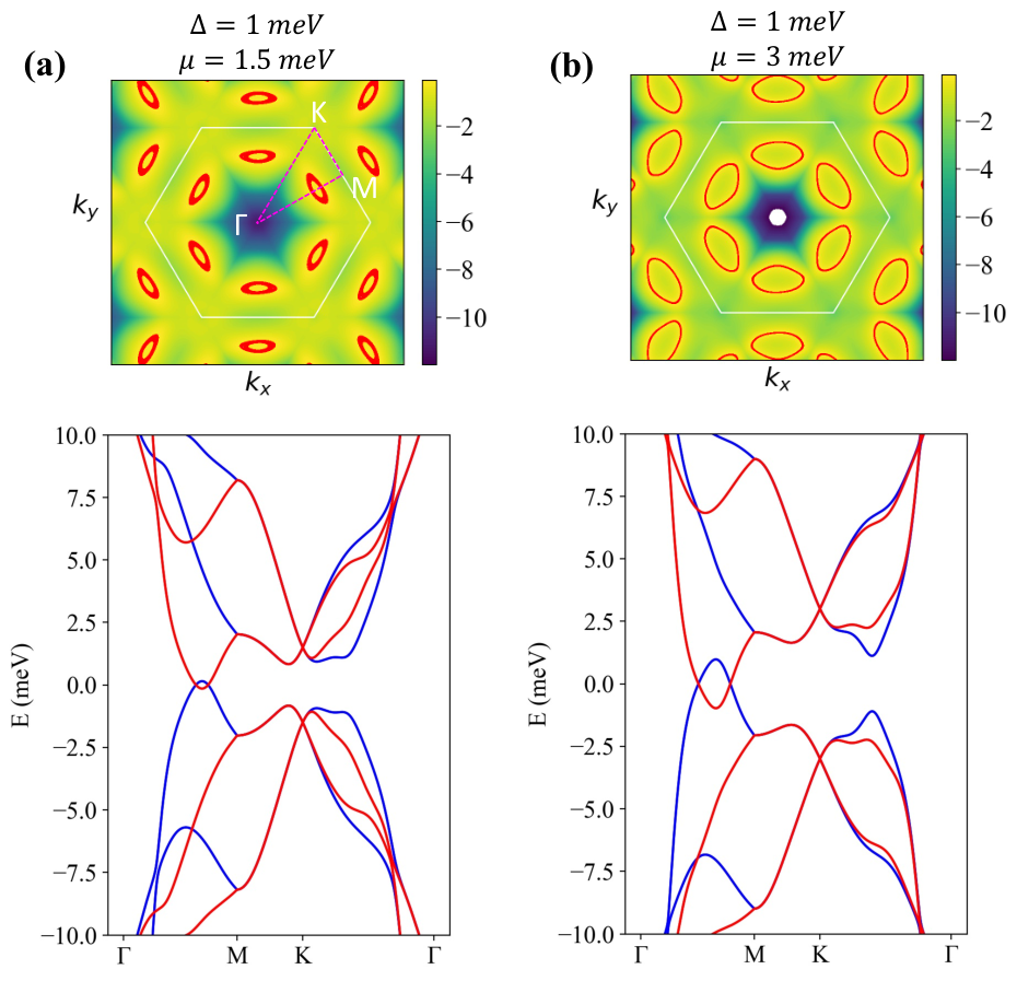
For VS pairing (both -symmetric and mirror-symmetric cases) in the TBG model, the BdG spectrum exhibits ring nodes in the region between the and points (hereafter referred as the midpoints). This is outside of the scope of the Dirac regime, which only applies to small value of momenta from the point. In short, the presence of the ring nodes is not protected by topology; instead, it is due to the band dispersion of the flat bands and the decoupling between the and valleys.
Consider the BdG Hamiltonian for intra-valley intra-sublattice pairing,
| (43) |
where again denotes the single-valley Hamiltonian adapted from Carr et al. 2019. In the above BdG Hamiltonian, only the Nambu and valley degree of freedom is shown explicitly; encapsulates matrix structure for the spin and sublattice degree of freedom. We note that the BdG Hamiltonian decouples into two sub-block matrix, one for each valley:
| (44) |
where and denotes the sub-block matrix corresponding to the up and down valleys respectively. Since the BdG Hamiltonian decouples into block matrices in the valley space, bands from opposite valleys can cross each other without any hybridization/avoided-crossing behaviors that gap out the spectrum.
The flat bands of the normal state TBG near the midpoint is very close to zero energy. Adding a nonzero or can push the band across the zero energy and results in the ring nodes. In Fig. 8, the line cut BdG spectrum is plotted with bands from the two valleys illustrated in different colors: when increasing chemical potential from [Fig. 8(a)] to [Fig. 8(b)], the bands from the two valleys cross over each other (near the midpoint) without any avoided-crossing, which matches our understanding that the two valleys are decoupled.
We will now explain why ring node only occurs for intra-valley pairings, but not in inter-valley pairings. There is a BdG chiral symmetry by composing the time-reversal symmetry with the BdG particle-hole symmetry/redundancy. As illustrated in Fig. 9, an essential difference between inter- and intra-valley pairings is that the BdG chiral symmetry acts across (within) the valley block structure for intra-valley (inter-valley) pairings. Therefore, with a nonzero chemical potential , BdG chiral symmetry pins the Dirac cones to in inter-valley pairings, whereas a Dirac cone in an intra-valley pairing is not necessarily pinned at , and may shift up or down (which gives a ring node) as long as its chiral copy shifts in the opposite direction.
Appendix E Phonon-mediated mechanisms
We base our analysis on Ref. Wu et al. 2018, where superconductivity mediated by in-plane phonon is described by the following interaction Hamiltonian:
| (45) | ||||
where and are the attractive interaction strength mediated by the and phonon modes respectively, and is a spinor in the valley (labeled by ) and sublattice (labeled by ) space.
The inter-valley pairing is energetically more favorable than the intra-valley pairing; therefore, intra-valley pairing are not considered in Ref. Wu et al. 2018. After expanding in terms of the valley and sublattice degree of freedom, and consider only Bardeen-Cooper-Schrieffer (BCS) pairing in the inter-valley channel, the Hamiltonian presented in Ref. Wu et al. 2018 is
| (46) | ||||
where we can identify the 1st term, , as S pairing mediated by the phonon mode; one may also view it as a pair hopping term. The 2nd term, is also S pairing, but it is mediated by the phonon mode; one may also view it as an inter-sublattice hopping term. The 3rd term, , is pairing mediated by the phonon mode.
| Pairing | ||
|---|---|---|
| inter-valley inter-sublattice () | No | Yes |
| inter-valley intra-sublattice (S) | Yes | Yes |
| intra-valley inter-sublattice (V) | Yes | No |
| intra-valley intra-sublattice (VS) | No | No |
On the other hand, we are interested in the question of what are all the possible pairing scenarios generated by various in-plane phonon modes, regardless of energetics. The interactive Hamiltonian given in Eq. (45) turns out to also give rise to intra-valley pairing term of the form
| (47) |
which is a V pairing mediated by the phonon mode. The phonon mode does not mediate any intra-valley pairing. In addition, neither the or phonon mediate a VS pairing. The full phonon-mediated pairing scenarios are summarized in Table 3.
References
- Zhang et al. (2009) H. Zhang, C.-X. Liu, X.-L. Qi, X. Dai, Z. Fang, and S.-C. Zhang, Nature Physics 5, 438 (2009).
- Hasan and Kane (2010) M. Z. Hasan and C. L. Kane, Rev. Mod. Phys. 82, 3045 (2010).
- Xia et al. (2009) Y. Xia, D. Qian, D. Hsieh, L. Wray, A. Pal, H. Lin, A. Bansil, D. Grauer, Y. S. Hor, R. J. Cava, and M. Z. Hasan, Nature Physics 5, 398 (2009).
- Chen et al. (2009) Y. L. Chen, J. G. Analytis, J.-H. Chu, Z. K. Liu, S.-K. Mo, X. L. Qi, H. J. Zhang, D. H. Lu, X. Dai, Z. Fang, S. C. Zhang, I. R. Fisher, Z. Hussain, and Z.-X. Shen, Science 325, 178 (2009).
- Qi and Zhang (2011) X.-L. Qi and S.-C. Zhang, Rev. Mod. Phys. 83, 1057 (2011).
- Schnyder et al. (2008) A. P. Schnyder, S. Ryu, A. Furusaki, and A. W. W. Ludwig, Phys. Rev. B 78, 195125 (2008).
- Kitaev (2009) A. Kitaev, AIP Conf. Proc. 1134, 22 (2009).
- Ryu et al. (2010) S. Ryu, A. P. Schnyder, A. Furusaki, and A. W. W. Ludwig, New Journal of Physics 12, 065010 (2010).
- Fu (2011) L. Fu, Phys. Rev. Lett. 106, 106802 (2011).
- Qi et al. (2009) X.-L. Qi, T. L. Hughes, S. Raghu, and S.-C. Zhang, Phys. Rev. Lett. 102, 187001 (2009).
- Read and Green (2000) N. Read and D. Green, Phys. Rev. B 61, 10267 (2000).
- Anderson and Morel (1961) P. W. Anderson and P. Morel, Phys. Rev. 123, 1911 (1961).
- Balian and Werthamer (1963) R. Balian and N. R. Werthamer, Phys. Rev. 131, 1553 (1963).
- Leggett (1975) A. J. Leggett, Rev. Mod. Phys. 47, 331 (1975).
- Volovik (2010) G. E. Volovik, The Universe in a Helium Droplet (Oxford University Press, 2010).
- Sato and Ando (2017) M. Sato and Y. Ando, Rep. Prog. Phys. 80, 076501 (2017).
- Fu and Kane (2008) L. Fu and C. L. Kane, Phys. Rev. Lett. 100, 096407 (2008).
- Murakami and Nagaosa (2003) S. Murakami and N. Nagaosa, Phys. Rev. Lett. 90, 057002 (2003).
- Wan et al. (2011) X. Wan, A. M. Turner, A. Vishwanath, and S. Y. Savrasov, Phys. Rev. B 83, 205101 (2011).
- Armitage et al. (2018) N. Armitage, E. Mele, and A. Vishwanath, Rev. Mod. Phys. 90, 015001 (2018).
- Li and Haldane (2018) Y. Li and F. Haldane, Phys. Rev. Lett. 120, 067003 (2018).
- Hosur et al. (2014) P. Hosur, X. Dai, Z. Fang, and X.-L. Qi, Phys. Rev. B 90, 045130 (2014).
- Meng and Balents (2012) T. Meng and L. Balents, Phys. Rev. B 86, 054504 (2012).
- Cao et al. (2018a) Y. Cao, V. Fatemi, S. Fang, K. Watanabe, T. Taniguchi, E. Kaxiras, and P. Jarillo-Herrero, Nature (London) 556, 43 (2018a).
- Lu et al. (2019) X. Lu, P. Stepanov, W. Yang, M. Xie, M. A. Aamir, I. Das, C. Urgell, K. Watanabe, T. Taniguchi, G. Zhang, A. Bachtold, A. H. MacDonald, and D. K. Efetov, Nature (London) 574, 653 (2019).
- Choi et al. (2019) Y. Choi, J. Kemmer, Y. Peng, A. Thomson, H. Arora, R. Polski, Y. Zhang, H. Ren, J. Alicea, G. Refael, F. von Oppen, K. Watanabe, T. Taniguchi, and S. Nadj-Perge, Nature Physics 15, 1174 (2019).
- Jiang et al. (2019) Y. Jiang, X. Lai, K. Watanabe, T. Taniguchi, K. Haule, J. Mao, and E. Y. Andrei, Nature (London) 573, 91 (2019).
- Kerelsky et al. (2019) A. Kerelsky, L. J. McGilly, D. M. Kennes, L. Xian, M. Yankowitz, S. Chen, K. Watanabe, T. Taniguchi, J. Hone, C. Dean, A. Rubio, and A. N. Pasupathy, Nature (London) 572, 95 (2019).
- Cao et al. (2021) Y. Cao, D. Rodan-Legrain, J. M. Park, N. F. Q. Yuan, K. Watanabe, T. Taniguchi, R. M. Fernandes, L. Fu, and P. Jarillo-Herrero, Science 372, 264 (2021).
- (30) For symmetry classes without a particle-hole or chiral symmetry, the invariant of the Hamiltonian is defined as that for the states below zero energy.
- Turner et al. (2012) A. M. Turner, Y. Zhang, R. S. K. Mong, and A. Vishwanath, Phys. Rev. B 85, 165120 (2012).
- Hughes et al. (2011) T. L. Hughes, E. Prodan, and B. A. Bernevig, Phys. Rev. B 83, 245132 (2011).
- Chiu et al. (2016) C.-K. Chiu, J. C. Teo, A. P. Schnyder, and S. Ryu, Rev. Mod. Phys. 88, 035005 (2016).
- Zondiner et al. (2020) U. Zondiner, A. Rozen, D. Rodan-Legrain, Y. Cao, R. Queiroz, T. Taniguchi, K. Watanabe, Y. Oreg, F. von Oppen, A. Stern, E. Berg, P. Jarillo-Herrero, and S. Ilani, Nature (London) 582, 203 (2020).
- Wong et al. (2020) D. Wong, K. P. Nuckolls, M. Oh, B. Lian, Y. Xie, S. Jeon, K. Watanabe, T. Taniguchi, B. A. Bernevig, and A. Yazdani, Nature (London) 582, 198 (2020).
- Song et al. (2021) Z.-D. Song, B. Lian, N. Regnault, and B. A. Bernevig, Phys. Rev. B 103, 205412 (2021).
- Coh and Vanderbilt (2016) S. Coh and D. Vanderbilt, “Python tight binding (PythTB),” (2016).
- Carr et al. (2019) S. Carr, S. Fang, H. C. Po, A. Vishwanath, and E. Kaxiras, Phys. Rev. Research 1, 033072 (2019).
- Cao et al. (2018b) Y. Cao, V. Fatemi, A. Demir, S. Fang, S. L. Tomarken, J. Y. Luo, J. D. Sanchez-Yamagishi, K. Watanabe, T. Taniguchi, E. Kaxiras, R. C. Ashoori, and P. Jarillo-Herrero, Nature (London) 556, 80 (2018b).
- Goerbig and Montambaux (2017) M. Goerbig and G. Montambaux, Proceedings - 18th Seminaire Poincare: Matiere de Dirac , 25 (2017).
- de Gail et al. (2011) R. de Gail, M. O. Goerbig, F. Guinea, G. Montambaux, and A. H. C. Neto, Phys. Rev. B 84, 045436 (2011).
- (42) We note that for intra-valley pairing, the Cooper pairs will transform nontrivially under the microscopic translation. Yet, in the moiré problem the microscopic translation becomes an internal valley- symmetry, which is broken by the intra-valley pairing.
- Po et al. (2019) H. C. Po, L. Zou, T. Senthil, and A. Vishwanath, Phys. Rev. B 99, 195455 (2019).
- Po et al. (2018) H. C. Po, H. Watanabe, and A. Vishwanath, Phys. Rev. Lett. 121, 126402 (2018).
- (45) We note, though, that strain is known to be significant in typical samples of twisted bilayer graphene, so there could also be extrinsic -breaking.
- (46) This is different from just interchanging the second and the fourth rows and columns, since the order of group operations matters.
- Wu et al. (2018) F. Wu, A. MacDonald, and I. Martin, Phys. Rev. Lett. 121, 257001 (2018).