A Parameter Estimation Method for Multivariate Aggregated Hawkes Processes
Abstract
It is often assumed that events cannot occur simultaneously when modelling data with point processes. This raises a problem as real-world data often contains synchronous observations due to aggregation or rounding, resulting from limitations on recording capabilities and the expense of storing high volumes of precise data. In order to gain a better understanding of the relationships between processes, we consider modelling the aggregated event data using multivariate Hawkes processes, which offer a description of mutually-exciting behaviour and have found wide applications in areas including seismology and finance. Here we generalise existing methodology on parameter estimation of univariate aggregated Hawkes processes to the multivariate case using a Monte Carlo Expectation Maximization (MC-EM) algorithm and through a simulation study illustrate that alternative approaches to this problem can be severely biased, with the multivariate MC-EM method outperforming them in terms of MSE in all considered cases.
Keywords Hawkes processes mutually-exciting processes aggregated data binned data MCEM algorithm
1 Introduction
Modern data acquisition systems in many applications collect vast amounts of data that can be characterised as time series. An area of particular interest is cyber-security, where network data are recorded and questions arise about the correlation structure and ‘excitational’ effects in and between the resulting time series. We aim to uncover trends within and between such time stamped event data, which we model using point processes. For this, we are particularly interested in the multivariate Hawkes process, which provides a model for ‘mutually exciting’ events. Introduced in Hawkes 1971b; Hawkes 1971a primarily to model the occurrence of seismic activity, multivariate Hawkes processes have found wide application to many disciplines due to their ability to model cross-excitation. In the case of financial data, multivariate Hawkes processes have been used to model the joint dynamics of trades and mid-price changes of the NYSE (Bowsher 2007) and an overview of literature surrounding the application of these processes to finance is given in Bacry et al. 2015. Additionally Hawkes processes have been considered within cyber-security for modelling of computer network traffic (Mark et al. 2019; Price-Williams and Heard 2019) and social media activity, for example in Kobayashi and Lambiotte 2016 where propagation of ‘Twitter cascades’ is considered.
As discussed in Shlomovich et al. 2020 practical limitations on storing or recording high resolution data results in an abundance of aggregated data, that is streams of counts of occurrences per time bin. We can use the counting process representation of a -variate point process to model this aggregated data. Let be the th continuous time count process () denoting the number of events until time where , for and for . We further denote
to be the aggregated (binned) process. Then the discrete-time vector process is given by
where and is the bin width. Here we develop and extend the methodology detailed in Shlomovich et al. 2020 to handle parameter estimation of multivariate aggregated Hawkes processes. We do this by considering the superposition of the multivariate count process. This is an elegant method which manages to replicate both the marginal and the cross-correlation structure of the true process. Results from a simulation study, comparing the extended MC-EM algorithm to both the INAR() and binned log-likelihood approximations are presented in Section 3. This method is shown to produce estimates with lower MSE than currently available alternatives. We additionally derive the Hessian of a multivariate Hawkes process with exponential kernel, required for optimization, and present this in Appendix A along with the gradient derived in Ozaki 1979.
1.1 Multivariate Hawkes Processes
Formally, the -dimensional Hawkes process is a class of stochastic process such that independently for each ,
where (Hawkes 1971b). It is characterized via its conditional intensity function (CIF) defined as
| (1) |
where is a -dimensional vector called the background intensity and is the non-negative excitation kernel such that for and given by a matrix of functions. In this way, the intensity at an arbitrary time-point is dependent on the history of the multivariate process allowing for both self and mutually exciting behavior. In simple cases, if for all and , then this is non-cross exciting behavior. That is the cross-covariances are equal to zero and whilst the processes may be self exciting, they are independent and thus not mutually exciting (Hawkes 1971b). Further, in the bivariate case if for all but for all then does not affect the likelihood of events in , but the converse does not hold. In this case we have one way interaction between the two processes involved.
The CIF from (1) can be written for an exponential kernel as
where , , , are known as the baseline, excitation and decay parameters, respectively. Assuming stationarity of the multivariate Hawkes process we have that the vector of stationary densities is
so that
where is the Fourier transform of the excitation kernel given by
Note that is commonly referred to as the branching ratio, typically denoted by , with the condition for stationarity being that the spectral radius (Hawkes 1971a).
2 Multivariate MCEM for Aggregated Hawkes Processes
In a continuous time framework, maximum likelihood estimation (MLE) can be used to estimate the model parameters from a set of exact multivariate events on the interval (Ozaki 1979) denoted
where is the maximum observation or simulation time, is the event in process , and is the total number of events in process . When we observe an aggregation of these latent continuous times to a count process of events per time bin, we lose information and in particular the likelihood of our observed event times given a parameter set can no longer be computed exactly due to reliance on the underlying time-stamps. In particular, the Hawkes process which is defined by its CIF, depends on the history of the process, which if ‘blurred’ by binning or rounding requires correct handling in order to obtain meaningful parameter estimates. In Shlomovich et al. 2020 an MC-EM (Monte Carlo Expectation Maximisation) algorithm for the parameter estimation of univariate aggregated Hawkes processes is presented. Here this work is extended for multivariate data.
2.1 The Monte Carlo EM Algorithm
The EM algorithm (Dempster et al. 1977) augments observed data by a latent quantity (Wei and Tanner 1990) to iteratively compute the maximizer of a likelihood. Here, the observed data are the multivariate event counts per unit time The latent data, are the unobserved, true event times. These are marked time-stamps which are not observed due to practical restrictions. We denote the parameter set to be , where is , and and are . The following two steps are as detailed in Shlomovich et al. 2020:
- 1.
In the E (Expectation) step, we compute
(2) where denotes the sample space for .
- 2.
In the M (Maximization) step, maximize the conditional expectation in (1) to obtain the updated parameter estimate, .
Monte Carlo methods can be used to numerically compute (1) if it is intractable, forming an algorithm known as MCEM (Wei and Tanner 1990). As we cannot sample the time-stamps directly we use importance sampling to simulate proposals for from a feasible alternative distribution, denoted .
Unique to the multivariate formulation is the need to retain the latent covariance structure between the processes. To this end, we sample the times of the univariate superposition of the -variate process. We then split the superposed simulated time-stamps to processes to create proposals matching the multivariate counts. We refer to such viable proposals as consistent. This approach is detailed further in Section 2.2. Once sampled, each proposal is weighted according to the probability it came from the desired distribution. That is, given a set of samples , we assign weights
| (3) |
and approximate (1) with
| (4) |
It is shown in Shlomovich et al. 2020 that if only proposing consistent event times
where is given in Daley and Vere-Jones 2003 by
2.2 Multivariate Sampling via the Superposition Process
Generating consistent time-stamps for the latent multivariate process such that the true covariance structure is captured is an important problem. We propose the following method for this, which allows us to extend the work in Shlomovich et al. 2020 for multivariate count data. Consider being a binned -variate Hawkes process with exponential kernel. In order to generate possible multivariate, continuous time proposal, , of the underlying event times, , we consider the superposed binned count process,
and reparameterize the multivariate parameter set to a corresponding set for the univariate superposed process , according to the kernel. We denote the adjusted parameter set for as .
It is given that the intensity of the superposed count process can be written as . The stationary intensity of the consistent proposed time-stamps is equal to that of the superposed observed counts, and so we have that
| (5) |
where and is the branching ratio of the superposed process, equal to in the case of an exponential kernel. We additionally note that . This can be seen by noting that
It remains to define a reparameterization for and . From Equation (5) and noting that , we have
| (6) |
Here we consider the exponential kernel where and thus we can use Equation (6) in order to retain a consistent stationary intensity in the univariate proposal.
We find that a suitable choice for is
for , and by Equation (6)
Empiricial studies show this reparameterization accurately recovers the true CIF of the superposed process. In this way we only simulate a univariate process, albeit a superposed version, and denote the simulated times as . In order to generate a realization of the multivariate Hawkes process, , with cross-covariances, we uniformly sample the observed number of events in each bin for each process from the . That is, we simulate a consistent set of continuous times for the superposed process matching the observed counts for , and then uniformly assign points within each bin to each of the processes. If desired, the allocation of events to the processes can be conducted times to generate multiple possible multivariate versions of the proposed realization of . If , the sample which maximises the log-likelihood is selected, otherwise the single multivariate proposal is taken and the MLE is used to estimate the parameters of the multivariate process from the continuous-time proposed realization. We present results for in Section 3.
This method provides us with an efficient way of artificially injecting cross-correlation into the consistent proposals whilst also retaining the marginal properties. In order to speed up the maximisation of the likelihood, we require the gradient and Hessian, given in Appendix A. The full algorithm for this multivariate approach is derived and presented in Appendix B.
2.3 Sampling Method
The question remains of how to best sample the latent times. The sequential simulation method detailed in Shlomovich et al. 2020 is applicable in the multivariate extension due to the reparameterization step meaning we need only sample times for the univariate superposition process. In this case, the normalised weight of the th Monte Carlo sample () is given by
| (7) |
where is the number of Monte Carlo samples. Further we note that
where is the log-likelihood of the sequentially sampled superposed times given the superposed counts and reparameterized univariate estimates, and denotes the probability of the random division of superposed time-points into a -variate count process matching the observed counts.
3 Simulation Study
We conduct a simulation study to compare the performance of the multivariate MC-EM algorithm to the INAR() method introduced in Kirchner 2016. We also compare the results to an approximation which ignores inter-bin excitation, referred to as the binned log-likelihood method. This approach represents the CIF as a piecewise constant function within each bin, equivalently assuming that , where are the counts in the th bin of the th process (Mark et al. 2019).
Given parameters a matrix, and and both being matrices, along with some maximum simulation time , we can simulate realizations of a Hawkes process. The generated events represent the underlying process and aggregating these to a chosen binning allows us to simulate the count data . We then apply each of the multivariate MC-EM methods, INAR() and binned log-likelihood approximation.
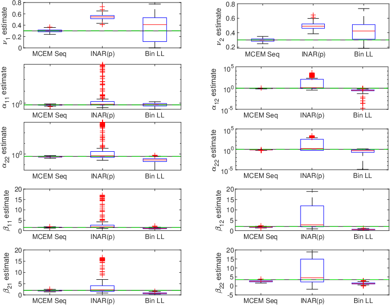
Boxplots for each of the ten estimated parameters used for characterising the bivariate Hawkes process are given in Figure 1. The parameters used for simulation are
with and . The parameters have been chosen as a stationary case with ample cross-excitation and non-symmetric self-excitation. The mean parameter estimates from repeated simulations is presented on the vertical axis. The INAR() approximation method can yield highly variable results, which is to be expected as the method is primarily intended for selecting a parametric kernel from continuous time data. The usual implementation of the INAR() involves selecting such that there is approximately one event per bin, however for our application this is not possible and so the choice of here is chosen to better reflect real data. A log-scale has been used in all four graphs relating to each of and . Both the binned log-likelihood, and particularly the INAR() method produced large outliers, resulting in very large MSE relative to the MC-EM approach. Tables 1 and 2 present summary statistics for the outlier-trimmed data. Specifically we remove the top and bottom 5% of parameter estimates for each of the three methods and report the relative bias, mean and standard deviation for each of the parameters and methods. We see that even after removing outliers and negative values from the INAR parameter estimates, the variability is much higher than that of the MC-EM. The absolute value of the bias of both the INAR and binned log-likelihood approaches is also larger than that of the MC-EM, in some cases significantly so. Overall, the proposed MCEM approach has much improved estimation performance than the other methods.
| Parameter | MCEM Rel. Bias | INAR() Rel. Bias | Binned LL Rel. Bias |
|---|---|---|---|
| Ground Truth | MCEM Mean (sd) | INAR() Mean (sd) | Binned LL Mean (sd) | MLE Mean (sd) | |||||
|---|---|---|---|---|---|---|---|---|---|
| (0.02) | (0.04) | 0.34 | (0.20) | (0.02) | |||||
| (0.018) | (0.036) | 0.409 | (0.099) | (0.016) | |||||
| (0.05) | (79.40) | 0.75 | (0.20) | (0.05) | |||||
| (0.06) | (394.00) | 0.29 | (0.09) | (0.08) | |||||
| (0.05) | (127.00) | 0.29 | (0.11) | (0.06) | |||||
| (0.06) | (236.00) | 0.49 | (0.33) | (0.09) | |||||
| (0.12) | (2.72) | 1.09 | (0.18) | (0.11) | |||||
| (0.14) | (5.56) | 0.55 | (0.14) | (0.18) | |||||
| (0.19) | (3.90) | 0.73 | (0.21) | (0.19) | |||||
| (0.29) | (5.93) | 1.37 | (0.32) | (0.41) | |||||
Evaluation of the methods is additionally explored via goodness of fit. This is an important aspect which allows us to check the validity of the estimates given the data. Often, the random change theorem, given in Daley and Vere-Jones 2003, is used for considering goodness of fit by transforming time-points using the compensator function
where is the event in process . In practice, is estimated using parameter estimates , and goodness of fit is conducted by considering the distribution of the transformed times, defined as . By the random time change theorem, is a realization of a unit rate Poisson process if and only if is a realization from the point process defined by .

Figure 2 shows QQ-plots relating to count processes from the simulation study and comparing the distribution of time-points transformed by each of the parameter estimates against those using the simulation parameters. We see that the estimates produced by the MC-EM algorithm are indeed a viable parameter set for this realization under an exponential Hawkes model, with the transformed time-points being distributed very close to those of the latent times. We also note that as the binned log-likelihood method ignores the effect of inter-bin excitation, it is expected that as the average number of counts in a bin increases, the fit from using this method will worsen.
4 Case Study
Network flow data, referred to as NetFlow, assembles records exported by routers and describes communications between devices connected to an enterprise network. Monitoring and analysing NetFlow data has been successful at detecting a range of malicious network behavior (Turcotte et al. 2018). Here we detect both self-exciting effects in the communication between a pair of network devices, termed here as an ’edge’, and mutually-exciting activity between such edges in the Los Alamos National Lab (LANL) enterprise network. By modelling the activity in this way, insight into the correlation structure of communications in the network can be obtained and monitored. We consider the methods outlined in Section 3 for parameter estimation of aggregated Hawkes processes as the NetFlow data is recorded at a 1 second resolution resulting in multiple events occurring simultaneously.

Figure 3 presents a selected pair of edges in the LANL network with possibe mutually-exciting Hawkes behavior in the communications over a duration of 45 minutes. We refer to the counts in blue as process 1 and the counts in red as process 2. The window selected is chosen as a period of more frequent events surrounded by no activity.

Parameter estimates are found using the MC-EM, INAR() and binned log-likelihood methods and performance is considered using goodness of fit. This allows us to assess whether the estimates represent viable parameters for modelling the observed data as a mutually-exciting Hawkes process. To do this, we use the time rescaling theorem discussed in Section 3. Figure 4 shows that the parameter estimates obtained via the MC-EM algorithm are likely viable parameters. The MC-EM parameter estimates are
The branching ratio, defined in Section 1.1 is therefore
where denotes element-wise division and is the average number of events in process directly triggered by each event in process .

These results indicate that there is mutually-exciting behavior between these processes in one direction such that process 2 does not affect process 1 but process 1 does affect process 2, where process 1 is presented in blue in Figure 3 and process 2 in red. There parameter estimates suggest that for each event in process 1, an average of 0.27 events will be triggered in process 2. The baseline parameters given by indicate the rate of the events is approximately one event every 100 seconds. Both processes are modelled with self-excitation, with each event in processes 1 and 2 triggering 0.34 and 0.28 events in their respective processes. Figure 5 shows the estimated excitation kernel components. From this we can see nature of the exciting effects, where illustrates the excitational effect which process has on process .
5 Conclusion
Here we have presented a novel method for generalising an MCEM algorithm to handle multivariate aggregated data. By reparameterizing our multivariate model in terms of the superposed process we can inject the necessary cross-covariance structure required for generating valid proposals. We also present closed form expressions for the gradient and Hessian of the log likelihood for increased computational efficiency. We further conducted a simulation study to compare this approach to the INAR() approximation detailed in Kirchner 2016 and a multivariate extension of the binned log likelihood method from Mark et al. 2019; Shlomovich et al. 2020. As in the univariate case, the MCEM method out-performed both alternatives in the presented parameter set and moreover, can vary provided the interval bounds are known. The multivariate extension can also be applied for other Hawkes kernels.
References
- Bacry et al. (2015) E. Bacry, I. Mastromatteo, and J.-F. Muzy. Hawkes processes in finance. Market Microstructure and Liquidity, 1(1), June 2015.
- Bowsher (2007) C. G. Bowsher. Modelling security market events in continuous time: Intensity based, multivariate point process models. Journal of Econometrics, 141(2):876–912, Dec. 2007.
- Daley and Vere-Jones (2003) D. J. Daley and D. Vere-Jones. An introduction to the theory of point processes. Springer, New York, 2nd edition, 2003.
- Dempster et al. (1977) A. P. Dempster, N. M. Laird, and D. B. Rubin. Maximum likelihood from incomplete data via the EM algorithm. Journal of the Royal Statistical Society. Series B (Methodological), 39:1–38, 1977.
- Hawkes (1971a) A. G. Hawkes. Point spectra of some mutually exciting point processes. Journal of the Royal Statistical Society. Series B (Methodological), 33(3):438–443, 1971a.
- Hawkes (1971b) A. G. Hawkes. Spectra of some self-exciting and mutually exciting point processes. Biometrika, 58(1):83–90, 1971b.
- Kirchner (2016) M. Kirchner. Hawkes and INAR() processes. Stochastic Processes and their Applications, 126(8):2494–2525, Aug. 2016.
- Kobayashi and Lambiotte (2016) R. Kobayashi and R. Lambiotte. TiDeH: Time-dependent Hawkes process for predicting retweet dynamics. In Tenth International AAAI Conference on Web and Social Media, Mar. 2016.
- Mark et al. (2019) B. Mark, G. Raskutti, and R. Willett. Network estimation from point process data. IEEE Transactions on Information Theory, 65(5):2953–2975, May 2019.
- Ozaki (1979) T. Ozaki. Maximum likelihood estimation of Hawkes’ self-exciting point processes. Annals of the Institute of Statistical Mathematics, 31(1):145–155, Dec. 1979.
- Price-Williams and Heard (2019) M. Price-Williams and N. A. Heard. Nonparametric self-exciting models for computer network traffic. Statistics and Computing, pages 1–12, May 2019.
- Shlomovich et al. (2020) L. Shlomovich, E. Cohen, N. Adams, and L. Patel. A Monte Carlo EM algorithm for the parameter estimation of aggregated Hawkes processes. arXiv:2001.07160 [stat], Jan. 2020. arXiv: 2001.07160.
- Turcotte et al. (2018) M. J. M. Turcotte, A. D. Kent, and C. Hash. Unified host and network data set. In Data Science for Cyber-Security, Security Science and Technology, pages 1–22. World Scientific, Nov. 2018. ISBN 978-1-78634-563-9.
- Wei and Tanner (1990) G. C. G. Wei and M. A. Tanner. A Monte Carlo implementation of the EM algorithm and the Poor Man’s Data Augmentation algorithms. Journal of the American Statistical Association, 85(411):699–704, 1990.
Appendix A Gradient and Hessian of Multivariate Continuous Time Hawkes Processes
The likelihood function of the multivariate Hawkes process is given by
where
where is defined as
and . This can recursively be defined as
Therefore, the gradient can be expressed by the following.
where
and .
We can also compute the Hessian for the continuous multivariate Hawkes likelihood. There are 15 categories to consider, given here.
where
and
This covers all cases required for the full Hessian matrix.
Appendix B Multivariate MC-EM Algorithm
Here we provide an algorithm for the parameter estimation of multivariate aggregated Hawkes processes via the MC-EM procedure.