LIMIT THEOREMS FOR DEPENDENT COMBINATORIAL DATA, WITH APPLICATIONS IN STATISTICAL INFERENCE
Somabha Mukherjee
A DISSERTATION
in
Statistics
For the Graduate Group in Managerial Science and Applied Economics
Presented to the Faculties of the University of Pennsylvania
in
Partial Fulfillment of the Requirements for the
Degree of Doctor of Philosophy
2021
Supervisor of Dissertation
| Bhaswar B. Bhattacharya, Assistant Professor of Statistics |
Graduate Group Chairperson
| Dylan Small, Class of 1965 Wharton Professor of Statistics |
Dissertation Committee
Bhaswar B. Bhattacharya, Assistant Professor of Statistics
Robin Pemantle, Professor of Mathematics
Nancy R. Zhang, Ge Li and Ning Zhao Professor, Professor of Statistics
LIMIT THEOREMS FOR DEPENDENT COMBINATORIAL DATA, WITH APPLICATIONS IN STATISTICAL INFERENCE
©COPYRIGHT
2021
Somabha Mukherjee
This work is licensed under the
Creative Commons Attribution
NonCommercial-ShareAlike 3.0
License
To view a copy of this license, visit
Dedicated to my parents, Tapas Mukherjee and Ruby Mukherjee
ACKNOWLEDGEMENT
First of all, I would like to thank my parents (Tapas Mukherjee and Ruby Mukherjee) for their unmatched effort in bringing me up to where I am today. Without their support and enthusiasm, it would not have been possible for me to pursue higher studies outside my home country, India, for the past five years. I would also like to thank my elder sister (Pausali Mukherjee) for always being my role model.
Higher studies and research are not all about talent and passion for the subject; it requires a thorough understanding of the academic system, too. In this context, I was extremely fortunate to have an advisor like Bhaswar, who not only gave me an extremely comprehensive knowledge of the research world, but also taught me how actual research should be done, by training me to handle all sorts of difficulties that arise while working on real problems. Bhaswar is more than an advisor to me. At countless times he seemed like an elder brother to me, who would give me incomparable mental and moral support to uplift my spirit, whenever I was going through difficult times during my PhD career. Doing research successfully throughout the past five years would not have been possible without his priceless help and advice.
I was very fortunate to collaborate with/learn from many wonderful Professors at Penn, such as Nancy, Robin, Dylan, Zongming and Jian. My independent research on statistical physics under Robin was the main factor that ignited my passion in this subject. The knowledge that I gathered from that course helped me immensely during my later works on inference in statistical physics models, which form the main part of this thesis. I gained my first experience in working on real statistical problems with concrete applications through a collaboration with Nancy. I would also like to thank Dylan, Zongming and Jian for sparing a lot of their time on academic discussions with me and giving me advice on various issues. I am also grateful to Professor Bodhisattva Sen from Columbia University and Professor Ayanendranath Basu from the Indian Statistical Institute for giving me research experience during my undergraduate and master years.
I would specially like to thank two of my collaborators, Jaesung Son and Divyansh Agarwal for their wonderful contributions in my joint works with them. Both Jaesung and Divyansh are extremely efficient researchers, and it was a priviledge for me to work with them. In fact, Chapters 2 and 3 in this thesis are outcomes of my joint work with Jaesung and Bhaswar. I was also fortunate to have collaborators like Marcus Michelen, Stephen Melczer and Arun Kuchibhotla who were my seniors at Penn, and are now assistant professors in reputed institutes. I would specially like to thank Arun for teaching me a lot of things in mathematical statistics. He was a person whom I could ask for help at any time, and in spite of being an extremely busy researcher himself, he would always promptly agree to help me. I would also like to thank my collaborators Sagnik Halder, Debaprartim Banerjee, Professor Sumit Mukherjee, Professor George Michailidis, Professor Rohit Patra and Professor Andrew Johnson for their crucial roles in my research career. Chapter 4 is created out of my ongoing joint work with Sagnik, George and Bhaswar.
Finally, I would like to mention three persons who influenced me the most in my academic life. One of them was my father’s co-worker Udayaditya Bhattacharya who introduced me to olympiad level mathematics for the first time when I was in high-school. Without him, I would not even be pursuing my career in mathematics and statistics. The second person is Professor S.M. Srivastava, who opened my eyes to the divine beauty of Mathematics by instilling within me a deep passion for logic and axiomatic set theory. At times, when he was teaching, it felt like I was learning from the great Georg Cantor or Kurt Gődel. He is the only reason behind my sublime love for mathematics. And the third person is Professor Alok Goswami who was the only person from whom I learned everything in Probability during my bachelor and master days, starting from counting balls in boxes to Itô calculus and general Markov processes. I owe my research career in probability to him.
Thank you,
Somabha Mukherjee.
ABSTRACT
LIMIT THEOREMS FOR DEPENDENT COMBINATORIAL DATA, WITH APPLICATIONS IN STATISTICAL INFERENCE
Somabha Mukherjee
Bhaswar B. Bhattacharya
The Ising model is a celebrated example of a Markov random field, which was introduced in statistical physics to model ferromagnetism. More recently, it has emerged as a useful model for understanding dependent binary data with an underlying network structure. This is a discrete exponential family with binary outcomes, where the sufficient statistic involves a quadratic term designed to capture correlations arising from pairwise interactions. However, in many situations the dependencies in a network arise not just from pairs, but from peer-group effects. A convenient mathematical framework for capturing higher-order dependencies, is the -tensor Ising model, which is a discrete exponential family where the sufficient statistic consists of a multilinear polynomial of degree . This thesis develops a framework for statistical inference of the natural parameters in -tensor Ising models. We begin with the Curie-Weiss Ising model, where every -tuple of nodes interact with equal strengths, where we unearth various non-standard phenomena in the asymptotics of the maximum-likelihood (ML) estimates of the parameters, such as the presence of a critical curve in the interior of the parameter space on which these estimates have a limiting mixture distribution, and a surprising superefficiency phenomenon at the boundary point(s) of this curve. However, ML estimation fails in more general -tensor Ising models due to the presence of a computationally intractable normalizing constant. To overcome this issue, we use the popular maximum pseudo-likelihood (MPL) method, which avoids computing the inexplicit normalizing constant based on conditional distributions. We derive general conditions under which the MPL estimate is -consistent, where is the size of the underlying network. Our conditions are robust enough to handle a variety of commonly used tensor Ising models, including spin glass models with random interactions and the hypergraph stochastic block model. Finally, we consider a more general Ising model, which incorporates high-dimensional covariates at the nodes of the network, that can also be viewed as a logistic regression model with dependent observations. In this model, we show that the parameters can be estimated consistently under sparsity assumptions on the true covariate vector.
TABLE OF CONTENTS
LIST OF ILLUSTRATIONS
Chapter 1 Introduction
The recent accumulation of dependent network data in modern statistics has made it increasingly important to develop realistic and mathematically tractable methods for modeling structure and dependence in high-dimensional distributions. Dependent data commonly arise in social and epidemic networks, spatial statistics, image databases, neural networks and computational biology. For example, in a social network like the facebook, the attributes of the users are dependent random variables, conditional on the underlying friendship network (Fig 1.1 (a)). This is because the probability that two people are friends, often depends on the similarity/dissimilarity between their attributes. The health status of individuals in an epidemic network is another example of highly correlated data. Another example of spatially correlated data is presidential election pattern across neighboring states. Figure 1.1 (b) shows the US neighborhood graph and outcome of the presidential election in the year 2012. Both the pictures in Figure 1.1 were kindly provided to me by Bhaswar Bhattacharya.
There is a massive amount of literature on how to analyze independent data in probability and statistics. However, there are many theoretical as well as practical scenarios, which demand analogous techniques for analyzing dependent data. For example, in an Erdős-Rényi random graph, where each edge is present with some fixed probability, independent of the other edges, the indicators corresponding to the occurrence of triangles and higher order motif counts, are dependent random variables. Hence, in order to describe the asymptotic behavior of the total number of triangles in an Erdős-Rényi random graph, one needs an asymptotic theory for the sum of dependent random variables. A more practical scenario arises in the estimation of the number of edges in a large, inaccessible network . A common strategy to do this is to sample some vertices at random from with probability , and count the number of edges in the graph induced by on the sampled vertices. One can then show that the statistic is an unbiased estimator of . Now, one can write
where denotes the indicator that both the nodes and in are sampled. Clearly, the collection is not independent, since for any three distinct nodes ,
So, once again, in order to derive theoretical properties of the estimator , one needs an asymptotic theory for the sum of dependent random variables.
Another common example of spatially correlated data are the pixels of an image. In order to get a smooth image, one would require adjacent pixels to be strongly correlated. In other words, any reasonable probability model on the pixels should favor a configuration of pixels, where neighboring pixels have similar or identical states [1]. An appropriate probability model for this setting can thus be described as
| (1.1) |
where is a configuration of pixel values, denotes that the pixels ands are neighbors, and the constant is a parameter depending on the image.
The model (1.1) is a special case of the more general (second order) Markov random field, given by:
| (1.2) |
where , , for some finite set , is a nonzero function, and is a nonzero symmetric function. For the model (1.1), , , and , where if and otherwise.
A special case of the Markov random field model (1.2) is the Ising model, which was initially developed in statistical physics to model ferromagnetism [59]. Although it was used initially as a framework for modeling interactions between particles sitting on the nodes of a network (Fig 1.2), recently the Ising model has turned out to be particularly useful for modeling various statistical datasets with an underlying network structure (cf. [3, 18, 26, 58, 23, 32] and the references therein). This is a discrete exponential family with binary outcomes, where the sufficient statistic involves a quadratic term designed to capture correlations arising from pairwise interactions and a linear term measuring the overall individual effect, and can be obtained from the model (1.2) by taking , , , and for some known symmetric matrix , known as the interaction matrix. and are treated as parameters of the Ising model, with acting as a measure of correlation between the variables , and acting as an overall signal strength. In the language of statistical physics, and are called the inverse temperature and the external magnetic field, respectively.

The -tensor (spin) Ising model, a specific instance of the more general higher-order Markov random fields, is a discrete exponential family where the sufficient statistic consists of a multilinear polynomial of degree and a linear term, which provides an effective and mathematically tractable way to simultaneously model both peer-group effects, between -tuples of friends, and individual effects. More precisely, the -tensor Ising model is given by:
| (1.3) |
for all and some known symmetric tensor , known as the interaction tensor. For various examples and applications of this and related models in statistical physics, see [4, 35, 39, 41, 42, 45] and the references therein.

The -tensor Ising model acts as a useful framework in situations where the dependencies in a network arise not just from pairs, but from peer-group effects. For example, it is more likely for an individual to choose a binary attribute if many groups of friends have also chosen the same attribute. In fact, we demonstrate this phenomenon on a music recommender system data in Chapter 3, where we show that users’ preference for a particular artist does not depend only on their pairwise interactions, but rather on higher order peer effects. A similar phenomenon also arises in various models of crystals, where the atoms on a crystal surface (see Fig 1.3) interact not just in pairs, but in triangles and higher order tuples.
1.1 Outline of the Thesis
In this thesis, we consider the problem of estimating the parameters and of the -tensor Ising model (1.3) given a single sample from the model. This problem has been extensively studied for the (matrix) case, which includes, among others, the classical results on consistency and optimality of the maximum likelihood (ML) estimates for lattice models [12, 25, 27, 36], and the seminal paper of Chatterjee [10], where general conditions for -consistency of the maximum pseudolikelihood estimate (MPLE) [5, 6] were derived. Various extensions and applications of the techniques in [10], in the contexts of estimation of parameters in matrix Ising models on general weighted graphs, logistic regression models with dependent observations, more general Ising models where the outcomes are influenced by various underlying networks, joint estimation of parameters, and related problems in hypothesis testing, can be found in [7, 17, 53, 14, 24, 9, 33].
However, none of these results say anything about the limiting distribution of the estimates, and hence, cannot be used for inferential tasks, such as constructing confidence intervals and hypothesis testing. In fact, proving general limit theorems in these models is often extremely difficult, if not impossible, because of the presence of an unknown normalizing constant (partition function) in the estimation objective function, which is both computationally and mathematically intractable for Ising models on general graphs. As a consequence, it is natural to assume certain special structures on the underlying network interactions if one desires to obtain precise results such as central limit theorems. A particularly useful structural condition which preserves several interesting properties of general systems, is to assume that all pairwise interactions between the nodes of the network are present. This is the well-known 2-tensor (matrix) Curie-Weiss model [19, 21, 22, 31], which has been extensively studied in physics, probability, and statistics, and provides the foundations of our understanding of mean-field models with pairwise interactions. In particular, Comets and Gidas [13] provided a complete description of the limiting distribution of the ML estimates of the parameters in the matrix Curie-Weiss model.
The matrix Curie-Weiss model naturally extends to the -tensor Curie-Weiss model, for any , in which the underlying tensor has all the possible -tuples of interactions. The -tensor Curie-Weiss model is a special case of (1.3), obtained by taking all entries of the interaction tensor to be . In Chapter 2, we establish highly non-standard asymptotics of the ML estimates in the -tensor Curie-Weiss model. In particular, we demonstrate the existence of a critical curve in the interior of the parameter space, on which the ML estimates have a limiting mixture distribution comprising of normals, half-normals and point masses. More surprisingly, we show that at the boundary points of this curve, the ML estimates are superefficient, converging at a rate faster than the parametric rate , to limiting non-Gaussian distributions. The geometry of this curve also depends on the parity of the interaction factor .
In more general Ising models, ML estimation is not possible due to the presence of an inexplicit and intractable normalizing constant in the expression of the likelihood function. To be precise, the normalizing constant for the measure (1.3) is given by:
Since is a sum of many terms, for even moderately large values of , it is incomputable in general (although in Chapter 2 we will see that this can be computed in time using the special structure of the Curie-Weiss network). This computational issue was circumvented by Chatterjee [10], who proposed using the maximum pseudolikelihood (MPL) estimator, which maximizes an approximation of the likelihood, obtained by taking product of the conditional distribution of each entry of given the rest, over all the entries of . In Chapter 3, we use the maximum pseudo-likelihood (MPL) method to provide a computationally efficient algorithm for parameter estimation that avoids computing the intractable partition function. We establish general conditions under which the MPL estimate is -consistent, that is, it converges to the true parameter at rate . Our conditions are robust enough to handle a variety of commonly used tensor Ising models, including spin glass models with random interactions and models where the rate of estimation undergoes a phase transition. In particular, this includes results on -consistency of the MPL estimate in the well-known -spin Sherrington-Kirkpatrick (SK) model, spin systems on general -uniform hypergraphs, and Ising models on the hypergraph stochastic block model (HSBM). In fact, for the HSBM we pin down the exact location of the phase transition threshold, which is determined by the positivity of a certain mean-field variational problem, such that above this threshold the MPL estimate is -consistent, while below the threshold no estimator is consistent. Finally, we derive the precise limiting distribution of the MPL estimate in the special case of the Curie-Weiss model, which is the Ising model on the complete -uniform hypergraph, at all points above its estimation threshold. Interestingly, in this case, the MPL estimate saturates the Cramer-Rao lower bound, showing that even though the MPL estimate is obtained by minimizing only an approximation of the true likelihood function for computational convenience, there is no loss in its asymptotic statistical efficiency.
In Chapter 4, we consider a more general model which incorporates the covariate information of the individual nodes. More precisely, it can be viewed as a generalization of the classical logistic regression model, with dependent observations. The model considered there, allows varying signal strength (external magnetic field) terms, where each of these signals is assumed to be the linear projection of some high-dimensional covariate along a fixed parameter vector. With only the signal terms present, we recover the classical high-dimensional logistic regression model, but the presence of a quadratic interaction term leads us to view this model both as an Ising model with covariates (a variant of the standard Ising model) and as a logistic regression with dependent observations (a variant of the vanilla logistic regression). This framework can be used to model the health status of individuals in an epidemic network, which are binary outcomes (healthy or ill) depending not only on the health status of neighboring individuals in that network, but also on personal health attributes like age, weight, diet, and immunity. In Chapter 4, we propose an -penalized maximum pseudolikelihood approach to estimate the high-dimensional parameter in the Ising model with covariates, and show that under a sparsity assumption on the true parameter vector, our algorithm recovers it at rate , where is the dimension of the covariates and is the number of observations (size of the network).
Chapter 2 Maximum Likelihood Estimation in the Tensor Curie-Weiss Model
00footnotetext: This chapter is a joint work with Jaesung Son and Bhaswar B. BhattacharyaIn this chapter, we study the problem of parameter estimation in the -tensor Curie-Weiss model, i.e. the model (1.3) where all -tuples of interactions are present, and have equal strength. Given natural parameters and , the -tensor Curie-Weiss model is a discrete exponential family on , defined as:
| (2.1) |
for . The normalizing constant, also referred to as the partition function, is determined by the condition , that is,
| (2.2) |
Denote by the log-partition function of the model. Hereafter, we will often abbreviate , and , by , and , respectively, when there is no scope of confusion. For discussions on the various thermodynamic properties of this model, which in the statistical physics literature is more commonly known as the ferromagnetic -spin model, refer to [4, 35, 41, 45].
In this chapter, we consider the problem of estimating the natural parameters and given a single sample from the -tensor Curie-Weiss model (2.1). One interesting feature of the Curie-Weiss model is that the partition function here can be computed in linear time, which is evident from the following alternative expression of :
This makes the likelihood function easily computable, and hence, maximum likelihood (ML) estimation is possible. It is well-known, since the model (2.1) has only one sufficient statistic (the sample mean ), that joint estimation of the parameters in this model is, in general, impossible. This motivates the study of individual (marginal) estimation, that is, estimating when is assumed to be known and estimating when is assumed to be known. As mentioned before, for the matrix Curie-Weiss model, this problem was studied in [13], where the limiting properties of the individual ML estimates were derived. In this chapter, we consider the analogous problem for the -tensor Curie-Weiss model, for . In particular, we derive precise limit theorems for the individual ML estimates of and , hereafter, denoted by and , at all the parameter points. In addition to providing a complete description of the asymptotic properties of the ML estimates, our results unearth several remarkable new phenomenon, which we briefly summarize below.
- •
For ‘most’ points in the parameter space, the ML estimates and are -consistent and asymptotically normal (Theorem 2 and Theorem 5). Here, the limiting variance equals the limiting inverse Fisher information, which implies that the ML estimates are, in fact, asymptotically efficient at these points (Remark 2.8.1.2). The variance of the limiting normal distribution can be easily estimated as well, hence, this result also provides a way to construct asymptotically valid confidence intervals for the model parameters (Section 2.4).
- •
More interestingly, there are certain ‘critical’ points, which form a 1-dimensional curve in the parameter space, where and are still -consistent, but the limiting distribution is a mixture with both continuous and discrete components. The number of mixture components is either two or three, depending on, among other things, the sign of one of the parameters and the parity of . In particular, at the points where the critical curve intersects the region , the scaled ML estimates and have a surprising three component mixture distribution, where two of the components are folded (half) normal distributions and the other is a point mass at zero (Theorem 4 and Theorem 7). This new phenomenon, which is absent in the matrix case, is an example of the many intricacies of the tensor model.
- •
Our results also reveal various other interesting phenomena, such as, inconsistency of in a region of the parameter space, and an additional (strongly) critical point, where is -consistent, but is not. These results, which are formally stated in Section 2.1, together provide a complete characterization of the limiting properties of the ML estimates in the -tensor Curie-Weiss model.
An important byproduct of our analysis is a precise description of the asymptotic distribution of the sample mean (magnetization) (Theorem 2), a problem which is of independent interest in statistical physics. While this has been extensively studied for the case, to the best of our knowledge this is the first such result for the higher order () Curie-Weiss model. The proofs require very precise approximations of the partition function and a careful understanding of the maximizers of a certain function at all points in the parameter space. One of the technical bottlenecks in dealing with tensor models is the absence of the ‘Gaussian transform’, which allows one to relate the partition function with certain Gaussian integrals, in models with quadratic sufficient statistics, as in the matrix Curie-Weiss model. This method, unfortunately, does not apply when , hence, to estimate the partition function we use a more bare-hands Riemann-sum approximation (see Section A.2 for details).
The rest of this chapter is organized as follows. We state our main results on the limiting distribution of the sample mean and the ML estimates in Section 2.1. The proof of the limiting distribution of the sample mean is described in Section 2.2. A proof overview for the asymptotic distributions of the ML estimates is given in Section 2.3. In Section 2.4 we describe how these limiting results can be used to construct confidence intervals for the model parameters. Various details of the proofs and other technical lemmas are given in the Appendix.
2.1 Statements of the Main Results
In this section we state our main results on the limiting properties of the sample mean and the ML estimates in the -tensor Curie-Weiss model. The asymptotics of the sample mean are described in Section 2.1.1. The limiting distributions of the ML estimates are presented in Section 2.1.2. Finally, in Section 2.1.3 we summarize our results in a phase diagram.
2.1.1 Limiting Distribution of the Sample Mean
The fundamental quantity of interest in understanding the asymptotic behavior of the -tensor Curie-Weiss model is the sample mean . As alluded to before, the limiting properties of has been carefully studied for the case [13, 21]. Here, we will consider the case , where, as discussed below, many surprises and interesting new phase transitions emerge.
In order to state the results we need a few definitions: For and , define the function as
| (2.3) |
where , for , is the binary entropy function. The points of maxima of this function will determine the typical values of and, hence, play a crucial role in our results. A careful analysis of the function (see Section A.3.1) reveals that it can have one, two, or three global maximizers in the open interval , which leads to the following definition:11 1 For a smooth function and , the first and second derivatives of at the point will be denoted by and , respectively. More generally, for , the -th order derivative of at the point will be denoted by .
Definition 1.
Fix and , and let be as defined above in (2.3).
- 1.
The point is said to be -regular, if the function has a unique global maximizer and .22 2 A point is a global maximizer of if , for all . Denote the set of all -regular points in by .
- 2.
The point is said to be -special, if has a unique global maximizer and .
- 3.
The point is said to be -critical, if has more than one global maximizer.
Note that the three cases above form a disjoint partition of the parameter space . Hereafter, we denote the set of -critical points by , and the set of points where has exactly two global maximizers by . We show in Lemma 34 that the set of points in form a continuous -dimensional curve in the parameter space (see also Figure 2.7 and Figure 2.8). Next, we consider points with three global maximizers, that is . To this end, define
| (2.4) |
Alternatively, Lemma 34 shows that is the smallest for which the point is -critical. Now, depending on whether is odd or even we have the following two cases:
- •
odd: In this case Lemma 32 shows that, for all points , the function has exactly two global maximizers, that is, .
- •
even: Here, Lemma 32 shows that there is a unique point , with as defined in (2.4), at which the function has exactly three global maximizers. For all other points in , has exactly two global maximizers, that is, . In the case, is even, we will refer to the point , or, equivalently, the point , as the -strongly critical point.33 3 Note that the point is defined for all (even or odd) as in (2.4). However, for odd, this point is -critical, but not -strongly critical (that means it belongs to ). On the other hand, for this point is 2-special (see discussion in Remark 2.1.1). Hereafter, when the need while arise to distinguish strongly critical points from other critical points, we will refer to a point which is -critical but not -strongly critical, as -weakly critical. Note that the collection of all -weakly critical points is precisely the set .
(a)
(b)
It remains to describe the structure of -special points. To this end, fix and define the following quantities:
| (2.5) |
Again, depending on whether is even or odd there are two cases:
- •
odd: In this case, Lemma 33 shows that there is only one -special point .
- •
even: Here, again from Lemma 33 and the symmetry of the model about , there are two -special points and .
These points are especially interesting, because, as we will see in a moment, here the sample mean has fluctuations of order and a non-Gaussian limiting distribution.
(a)
(b)
The plots in Figure 2.1 and Figure 2.2 show instances of the different cases described above: Figure 2.1(a) shows the plot of the function at the -regular point , and Figure 2.1(b) shows the plot of the function at the -special point . On the other hand, Figure 2.2(a) shows the plot of the function at the -critical point , which has two global maximizers, and Figure 2.2(b) shows the plot of the function at the -strongly critical point , where the function has three global maximizers. In fact, recalling that denotes the set of all -regular points and the set of points where has exactly two maximizers, the discussion above can be summarized as follows:
Figure 2.7 and Figure 2.8 illustrates this decomposition of the parameter space for and , respectively.
Remark 2.1.1 Note that (2.1.1) provides a complete characterization of the parameter space for . As mentioned before, in the well-studied case of , the situation is relatively simpler [19, 21]. In this case, can have at most two global maximizers, that is, it has no strongly critical points, hence, . In fact, it follows from [21] that the set of points with exactly two global maximizers is the open half-line . Moreover, there is a single 2-special point (where there the function has a unique maximum, but the double derivative is zero), and all the remaining points are 2-regular. This shows that for there is no point in with that is critical. In contrast, for odd, the set of critical points is a continuous curve in which intersects the line at a single point, and for even, the set of critical points is a continuous curve in which has two arms that intersect the line in the half-line (see Lemma 34 for the precise statement and Figures 2.7 and 2.8 for an illustration.) Moreover, this curve has exactly one limit point (if is odd) and exactly two limit points (if is even) outside it, which is (are) precisely the -special point(s).
Having described the behavior of the function , we can now state the limiting distribution of , which depends on whether the point is regular, critical, or special.
Theorem 1 (Asymptotic distribution of the sample mean).
Fix and , and suppose . Then with as defined in (2.3), the following hold:
-
Suppose is -regular and denote the unique maximizer of by . Then, as ,
(2.8) -
Suppose is -critical and denote the maximizers of by . Then, as ,
(2.9) where for each ,44 4 Note that all the global maximizers of the function belong to the open interval , and if is -critical and are the global maximizers of , for some , then , for all . These statements are proved in Lemma 32 and Lemma 33, respectively. This implies that the probabilities in (2.10) are well-defined. Moreover, when is -strongly critical, that is, has three global maximizers, the symmetry of the model about (recall that is even and for a strongly critical point), implies that the three maximizers are , for some .
(2.10) Moreover, if is an interval containing in its interior for some , such that for all , then
(2.11) -
Suppose is -special and denote the unique maximizer of by . Then, as ,
where the density of with respect to the Lebesgue measure is given by
(2.12) with denoting the fourth derivative of the function .
The result in Theorem 1 follows from a slightly more general version (see Theorem 8 in Section 2.2), where, instead of deriving the limiting distribution of at a fixed point , we compute the limits at appropriately perturbed parameter values , with and . This generalization will be required for deriving the asymptotic distribution of the ML estimates of and , described in the following section. Deferring the technical details for later, we describe below the key ideas involved in the proof of Theorem 1:
- •
In the -regular case, the proof has three main steps: The first step is to prove a concentration inequality of in an asymptotically vanishing neighborhood (Lemma 1). This not only shows that is the typical value of , but also implies that the partition function (which is the sum over all as in (2.2)), can be restricted over those for which lies within this concentration interval around . The second step is to find an accurate asymptotic expansion of by first approximating this restricted sum by an integral over the concentration interval, and then applying saddle point techniques to get a further approximation to this integral (Lemma 2). The third and final step is to use this approximation of to compute the limit of the moment generating function of , and show that the limit converges to that of the Gaussian distribution appearing in (2.8). Details are given in Section 2.2.1.
- •
The proof in the -special case follows the same strategy as the -regular case, with appropriate modifications to deal with the vanishing second derivative at the maximizer. As before, the first step is to prove the concentration of within a vanishing neighborhood of which, in this case, requires a higher-order Taylor expansion, since (Lemma 5). The second step, as before, is the approximation of the partition function (Lemma 6). The proof is completed by calculating the limit of the moment generating function of using this approximation to the partition function. Details are given in Section 2.2.2 and Section 2.5.
- •
For the -critical case, the basic proof strategy remains the same as above. However, to deal with the presence of multiple maximizers, we need to prove a conditional concentration result for the sample mean, that is, concentrates at one of the maximizers, given that lies in a small neighborhood of that maximizer (Lemma 3). Similarly, for the second step, we need to approximate a restricted partition function, where instead of taking a sum over all configurations as in (2.1), we sum over configurations such that lies in the neighborhood of one of the maximizers (Lemma 4). Details are given in Section 2.2.3 and Section 2.6.
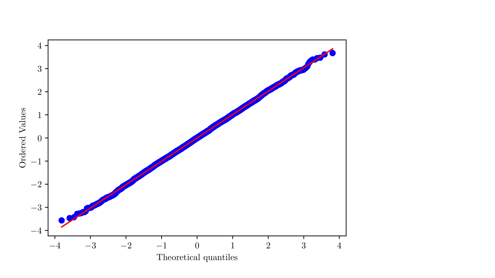
To empirically validate the different results in Theorem 1, we fix , some , and . Then we generate replications from and plot the histograms of the sample means. Figure 2.3(a) shows the histogram of at the -regular point where, as expected from (2.8), we see a limiting normal distribution. This is also confirmed from the corresponding quantile-quantile (QQ) plot in Figure 2.3(b). Next, Figure 2.4(a) shows the histogram of at the -special point , where a non-normal shape emerges, as predicted by (2.12). The non-normality is also confirmed from the QQ plot in Figure 2.4(b). Figure 2.5 shows the histogram of at the -critical point , where the function has two global maximizers (see plot in Figure 2.2(a)). Hence, the histogram of has two peaks located at two maximizers (as shown in (2.9)). Finally, in Figure 2.6 we show the histogram of at a -strongly critical point . Here, the histogram has three peaks, since the function has three global maximizers (see plot in Figure 2.2(b)). Note that the histograms of both in Figure 2.5 and 2.6, look like a Gaussian distribution in a neighborhood of each of the maximizers, as predicted by (2.11) in the theorem above.
(a)
(b)
(a)

(b)


2.1.2 Asymptotics of the ML Estimates
In this section we consider the problem of estimating the parameters and given a single sample using the method of maximum likelihood. Note that the distribution of the -tensor Curie-model (2.1) has a single sufficient statistic . This suggests, as mentioned before, that the parameters cannot be estimated simultaneously. In fact, one can show that the joint ML estimates for might not exist with probability 1 (see Lemma 37 for details). However, it is possible to marginally estimate one of the parameters assuming that the other is known. Hereafter, given , we denote by and the maximum likelihood estimators of and , respectively. Note that, for fixed , is a solution of the equation (in )
| (2.13) |
Similarly, for fixed , is a solution of the equation (in )
| (2.14) |
The limiting properties of the ML estimates of and are presented in Section 2.1.2.1 and Section 2.1.2.2, respectively. The full phase diagrams summarizing the results are given in Section 2.1.3.
2.1.2.1 ML Estimate of
In order to describe the asymptotic distribution of the ML estimate of , we need the following definition:
Definition 2.
For , the positive half-normal distribution is defined as the distribution of , where . The negative half-normal distribution is defined as the distribution of , where .
The asymptotic distribution of the ML estimate of is summarized in the theorem below. As expected, the results depend on whether is regular, critical, or special, which we state separately in the theorems below. In this regard, denote by the point mass at . We begin with the case when is regular. Throughout, will be as defined in (2.3).
Theorem 2 (Asymptotic distribution of at -regular points).
Fix and suppose is -regular. Assume is known and . Then denoting the unique maximizer of by , as ,
| (2.15) |
This result shows that is -consistent and asymptotically normal at the regular points. Before discussing more about the implications of this theorem, we state the result for the asymptotic distribution of when is -special.
Theorem 3 (Asymptotic distributions of at -special points).
Fix and suppose is -special. Assume is known and . Then denoting the unique maximizer of by , as ,
| (2.16) |
where the distribution function of is given by
with as defined in (2.34) below.
Finally, we consider the case is -critical. Here, it is convenient to consider the cases is odd or even separately.
Theorem 4 (Asymptotic distribution of at -critical points).
Fix and suppose is -critical. Assume is known and . Denote the maximizers of by , and let be as in (2.10).
-
Suppose is odd. In this case, the function has exactly two (asymmetric) maximizers and, as ,
(2.17) where are the half-normal distributions as in Definition 2.
-
Suppose is even. Then the following hold:
-
If , then the function has exactly two (asymmetric) maximizers and, as ,
-
If and , then the function has exactly two symmetric maximizers , where , for some . Then, as ,
(2.19) -
If and , the function has three maximizers , , and , where . Then, as ,
(2.20) where is as defined in (2.10).
-
The proofs of these results are given in Section 2.8 (a short roadmap of the proof is given in Section 2.3). The results above show that for all points in the parameter space, the ML estimate is a consistent estimate of , that is, . Moreover, the rate of convergence is , except at the -special points. However, at the -special point(s), the rate improves to , that is, the ML estimate of at these point(s) is superefficient, converging to the true value of faster than the usual rate at the neighboring points. Another interesting feature is that, while at the regular points has a simple Gaussian limit, at the critical points it has a mixture distribution, consisting of (half) normals and a point mass at . The reason the limiting distribution has a point mass at is because the sample mean is “discontinuous” under the perturbed measure , as transitions from negative to positive. In fact, Lemma 9 (in Section 2.7) shows that under the measure , the point where concentrates depends on the sign of the perturbation factor . Therefore, since the distribution function of evaluated at depends on the law of under the perturbed measure (see the calculations in Section 2.8.2 for details), it has a discontinuity at the point , and, hence, a point mass at appears in the limit.
Another interesting revelation are the results in (2.17) and ( ∙ ‣ ( 2 ) ), where the function has two (asymmetric) maximizers. In this case, the ML estimate converges to a three component mixture, which has a point mass at zero with probability and is a mixture of two half normal distributions, with probabilities and , respectively. This corresponds to the region of the critical curve where (and also the point , for odd), a striking new phenomena that emerges only when . Note that, this does not happen for , because, in this case, , hence, the two maximizers at any 2-critical point are symmetric about zero, and the two half normal mixing components combine to form a single Gaussian, and the resulting limit is the mixture of a single normal and a point mass at zero, as is the case in (2.19) above.
2.1.2.2 ML Estimate of
Here, we consider the ML estimate of . As before, the results depend on whether is regular, critical, or special. However, the analysis here is more involved, and each of these cases breaks down into further cases, depending on the value of the maximizers, the parity of , and the sign of . We begin with the case when is regular. As always, will be as defined in (2.3).
Theorem 5 (Asymptotic distributions of at -regular points).
Fix and suppose is -regular. Assume is known and . Then denoting the unique maximizer of by , the following hold,
-
If , then, as ,
(2.21) -
If , (equivalently, and ), then, as ,
(2.22) where with .
We will discuss the various implications of the above theorem later in this section. Now, we state the result for the asymptotic distribution of when is -special.
Theorem 6 (Asymptotic distributions of at -special points).
Fix and suppose is -special. Assume is known and . Then denoting the unique maximizer of by , as ,
| (2.23) |
where the distribution function of is given by
with as defined in (2.34) below.
Finally, we consider the case is -critical. The situation here is quite delicate, depending on various things like weak and strong criticality, parity of , and the sign of the field .
Theorem 7 (Asymptotic distribution of at -critical points).
Fix and suppose is -critical. Assume is known and . Denote the maximizers of by , and let be as in (2.10).
-
Suppose is odd. In this case, the function has exactly two maximizers . Then, as , the following hold:
-
If , where is defined in (2.4), then
-
If , then
(2.25)
-
-
Suppose is even. Then the following hold, as :
-
If , then
-
If , then
-
If and , there are exactly two maximizers and of , where . In this case,
(2.28) -
If and , there are exactly three maximizers , , and of , where . In this case,
where and is a standard normal random variable.
-
The proofs of the above results are given in Section 2.8. One of the main technical ingredients is a strengthening of Theorem 1, which requires obtaining the asymptotic distribution of when the parameters are perturbed by an term. A more detailed overview of the proof technique is given in Section 2.3. Here, we summarize the main consequences of the above results and highlight the various new phenomena that emerge as one moves from the matrix to the tensor case.
- •
For -regular points, Theorem 5 shows that when the unique maximizer , then is consistent at rate with a limiting normal distribution. On the other hand, when , which happens in the interval , the ML estimate is inconsistent. In this regime, when is odd, then concentrates at with probability , irrespective of the value of true value of . The situation is even more strange when is even. Here, concentrates at either or escapes to negative infinity, that is, with positive probability is unbounded, when and . The corresponding results for are similar in the sense that, for (recall that ), the ML estimate is inconsistent. However, unlike in the case for even, the ML estimate , when , is always finite and converges to a (properly centered and rescaled) chi-squared distribution [13, Theorem 1.4].
- •
For -special points Theorem 6 shows that converges to at rate , that is, it is superefficient. Recall that the same thing happens for at -special points (Theorem 3). In comparison, for at the only 2-special , is superefficient with rate [13, Theorem 1.3], but remains -consistent [13, Theorem 1.4]. This is because when is -special, the unique maximizer of is when , but non-zero, for . This creates a difference in the rate of convergence of the maxima of towards the maximum of for some suitably chosen perturbation of , which is an important step in deriving the asymptotic rate of convergence of the ML estimates. Another interesting difference is that for , the only 2-special point coincides with the thermodynamic threshold of the 2-tensor Curie-Weiss model. However, for , the -special points (the point , for odd, and the points , for even), where we get the non-Gaussian limits of , , and , have nothing to do with the thermodynamic threshold of the -tensor Curie-Weiss model, but rather depends on the vanishing property of the second derivative of at its maximizer. On the contrary, quite remarkably, the thermodynamic threshold of the -tensor Curie-Weiss model (recall definition in (2.4)) turns out to be a -weakly critical point for odd, and the only -strongly critical point for even, another unexpected phenomenon unearthed by our results.
- •
The landscape is much more delicate for -critical points, as can be seen from Theorem 7. In this case, the limiting distribution of converges to various mixture distributions, depending on, among other things, the sign of and the parity of . As in the case of , a particularly interesting new phenomena is the three component mixture that arises in the limiting distribution of when the critical curve intersects the region . This corresponds to the result ( ∙ ‣ ( 1 ) ) for odd, and results in ( ∙ ‣ ( 2 ) ) and ( ∙ ‣ ( 2 ) ) for even. Recall, from the discussion following Theorem 4, that this does not happen for , because, in this case, , hence, the two maximizers at any 2-critical point are symmetric about zero, and the two half normal mixing components combine to form a single Gaussian. As a result, the limit is the mixture of a single normal and a point mass at zero. Interestingly, this also happens for even, when the critical curve intersects the line and is strictly above the threshold , as seen in (2.28) above.
- •
The final bit in the puzzle is the point of thermodynamic phase transition . Here, the ML estimate is not -consistent. More precisely, in the limit, has a point mass at negative infinity with positive probability, and is a mixture of a folded normal and a point mass with the remaining probability (as described in (2.25) and ( ∙ ‣ ( 2 ) )). In contrast, as explained in the second case above, when , then at the point of thermodynamic phase transition () the ML estimate is -consistent.
2.1.3 Summarizing the Phase Diagram
The results above can be compactly summarized and better visualized in a phase diagram, which shows the partition of the parameter space described in (2.1.1). The phase diagrams for and , obtained by numerical optimization of the function over a fine grid of parameter values, are shown in Figure 2.7 and Figure 2.8, respectively. The limiting distributions that arise in the different regions of the phase diagram are described in the figure legends.
-
- –
- –
- –
- –
The curve: These are -weakly critical points where . Here, has two global (non-symmetric) maximizers. Both and are -consistent and asymptotically a three component mixture (comprising of two half normal normal distributions and a point mass at zero), by ( ∙ ‣ ( 2 ) ), ( ∙ ‣ ( 2 ) ), and ( ∙ ‣ ( 2 ) ), respectively.
- –
- –
-
- –
- –
- –
- –
- –
2.2 Asymptotic Distribution of the Sample Mean: Proof of Theorem 1
In this section, we will prove Theorem 1 in the -regular case and present proof roadmaps for the remaining two cases. To this end, note that the model (2.1) can be written more compactly as
where is the sample mean. Therefore, the sample mean has the probability mass function,
Observe that the expression for the probability mass function of involves the partition function , which does not have a closed form.55 5 Note that even though the partition function has no closed form, for a given value of it can be easily computed in time. This is one of the major advantages of the Curie-Weiss model, which allows, among other things, efficient computation of the ML estimates. Therefore, obtaining limiting properties of requires accurate estimation of . Moreover, as mentioned before, with the goal of deriving the limiting distribution of the ML estimates of and , we will need to prove the limiting distribution of at slightly perturbed parameter values , for some sequences and to be chosen later. Hereafter, we will denote , and , by , and , respectively. The asymptotic distribution of in the different cases at the appropriately perturbed parameter values is summarized below:
Theorem 8 (Asymptotic distribution of under perturbed parameters).
Fix , , and . Then with as defined in (2.3) the following hold:
-
Suppose is -regular and denote the unique maximizer of by . Then, for , as ,
(2.30) -
Suppose is -critical and denote the maximizers of denoted by . Then, for , as ,
(2.31) where are as defined in (2.10). Moreover, if is any local maximizer of contained in the interior of an interval , such that for all , then for , as ,
(2.32) -
Suppose is -special and denote the unique maximizer of by . Then, for , as ,
(2.33) where density of with respect to the Lebesgue measure is given by
(2.34)
Note that Theorem 1 follows directly from the above by taking and . We prove Theorem 8 in the -regular case in Section 2.2.1 below. The roadmaps of the remaining two cases, which follow a similar strategy but requires more a delicate analysis, are described in Section 2.2.2 and Section 2.2.3. The complete proofs of (2.32) and (2.33) are given in Section 2.6 and 2.5, respectively.
2.2.1 Proof of Theorem 8 when is -regular
Fix a -regular point and consider a sequence (to be specified later) such that and . It has been shown in Lemma 35 that the function will have a unique global maximizer , for all large , and as . Choose this maximizer and define, for ,
| (2.35) |
The first step in the proof of Theorem 8 when is -regular, is to show that under , the sample mean concentrates around at rate , for any .
Lemma 1.
Suppose is -regular. Then for and as defined above in (2.35),66 6 For any set , denotes the complement of the set .
Proof.
Note that the support of the magnetization is the set
It follows from [40], Equation (5.4), that for any , the cardinality of the set
can be bounded by
| (2.36) |
for some universal constant (recall that is the binary entropy function). Hence, we have from (2.36),
| (2.37) |
By Lemma 45, we know that for all large , is either or . Since and the functions are uniformly bounded on any closed interval contained in , Taylor’s theorem gives us:
| (2.38) | ||||
| (2.39) |
Note that (2.39) follows from (2.38) since . The proof of Lemma 1 is now complete, in view of (2.2.1). ∎
Lemma 1 shows that almost all contribution to comes from configurations whose average lies in a vanishing neighborhood of the maximizer of . This enables us to accurately approximate the partition function . This involves a Riemann approximation of the sum of the mass function over all whose mean lies in a vanishing neighborhood of , followed by a further saddle-point approximation of the resulting integral.
Lemma 2.
Suppose is -regular. Then for and large enough, the partition function can be expanded as,
| (2.40) |
where is the unique maximizer of the function . Moreover, for large enough, the log-partition function can be expanded as,
| (2.41) |
Proof.
Without loss of generality, let and note that
| (2.42) |
By Lemma 1, and hence (2.42) gives us
| (2.43) |
where is defined as
| (2.44) |
where is interpreted as a continuous binomial coefficient (refer to Section A.1 for the definition of continuous binomial coefficients). The next step is to approximate the sum in (2.2.1) by an integral, using Lemma 28. Note that Lemma 28 can be applied with to obtain (using Lemma 40),
| (2.45) |
It now follows from (2.2.1), Lemma 31, Lemma 29 and Lemma 39, that
| (2.46) |
Combining (2.2.1) and (2.2.1), we have:
| (2.47) |
This completes the proof of (2.40). If we take logarithm on all sides in (2.2.1) and use the fact that for any sequence , then we get (2.41), completing the proof. ∎
Completing the Proof of (2.30): We now have all the necessary ingredients in order to derive the CLT for when is -regular. Throughout this subsection, we take
for some fixed and . Now, recall that and is the unique maximizer of . To complete the proof we will show that the moment generating function of under converges pointwise to the moment generating function of the Gaussian distribution with mean and variance . Towards this, fix and note that the moment generating function of at can be expressed as
| (2.48) |
Using Lemma 2 and the fact that , the right side of (2.48) simplifies to
| (2.49) |
Now, Lemma 38 and a simple Taylor expansion gives us
Using (2.2.1) and a further Taylor expansion, we have
| (2.51) |
Next, we have by Lemma 38 and a Taylor expansion,
| (2.52) |
Adding (2.2.1) and (2.2.1), we have:
| (2.53) |
Using (2.2.1), the expression in (2.49) becomes
| (2.54) |
The constant in expression (2.54) is easily recognizable as the moment generating function of evaluated at . This completes the proof of Theorem 8. ∎
2.2.2 Proof Roadmap of Theorem 8 when is -special
When is -special, we consider local perturbations of the parameters
as in the statement of Theorem 8 (3). Note that in this case the function still has a unique maximizer , but . The proof strategy here follows essentially the same roadmap as in the -regular case, with relevant modifications while taking Taylor expansions, since . As before, the first step is to prove the concentration of within a vanishing neighborhood of (Lemma 5). Here, the concentration window turns out to be a little more inflated, that is, its length is of order , for . Next, we approximate the partition function , where, since the second derivative of is zero at the maximizer, we need to consider derivatives up to order four to accurately approximate (Lemma 6). The details of the proof are given in Section 2.5.
2.2.3 Proof Roadmap of Theorem 8 when is -critical
Throughout this section we assume that is -critical. This means, by definition and Lemma 32, that the function has global maximizers, which we denote by . It also follows from Lemma 35, that for sequences and , the function , for all large , have local maximizers such that , as , for all . As before, and will denote and , respectively.
In presence of multiple global maximizers, the magnetization will concentrate around the set of all global maximizers. In fact, we can prove the following stronger result: Consider an open interval around a local maximizer such that is the unique global maximizer of over . Then conditional on the event (which is a rare event if is not a global maximizer), concentrates around . This is the first step in the proof of Theorem 8 when is -critical. To state the result precisely, assume that is a local maximizer of and let be local maximizers of converging to , which exist by Lemma 35. Define
| (2.55) |
The following lemma gives the conditional and, hence, the unconditional, concentration result of around local maximizers.77 7 The unconditional concentration derived in (2.57) is not required in the proof of Theorem 8. Nevertheless, we include it for the sake of completeness. The proof is given in Section 2.6.1.
Lemma 3.
Suppose is -critical. Then for fixed and as defined in (2.55),
| (2.56) |
for any interval such that and , for all 88 8 For any set , and denote the topological interior and closure of , respectively. As a consequence, for ,
| (2.57) |
In order to derive a conditional CLT of around the local maximizer , given that is in (where is as in Lemma 3 above), we need precise estimates of the restricted partition functions defined as
Note that is the partition function of the conditional measure , in the sense that for any such that , we have
The following lemma gives an approximation of the restricted and, hence, the unrestricted partition functions. To this end, recall that is a local maximizer of converging to .
Lemma 4.
Suppose is -critical. Then for and large enough, the restricted partition function can be expanded as
| (2.58) |
where the set is as in Lemma 3. This implies, for every and large enough, the (unrestricted) partition function can be expanded as
| (2.59) |
The proof of this result is given in Section 2.6.2. We can now use the results above to complete the proof of Theorem 8 (2).
Completing the Proof of Theorem 8 when is -critical: For each and , define . Then for all small enough, , for all . Now, for each , we have
| (2.60) |
By Lemma 4 we have
| (2.61) |
and
| (2.62) |
The result in (2.31) now follows from (2.60), (2.61) and (2.62).
Now, we proceed we prove (2.32). Hereafter, let and . A direct calculation reveals that
| (2.63) |
Using Lemma 4, the right side of (2.63) simplifies to
where and are the local maximizers of the functions and respectively, converging to . We can mimic the proof of Theorem 8 verbatim from this point onward, to conclude that as ,
| (2.64) |
2.3 Asymptotic Distribution of the ML Estimates: Proof Overview
Here, we provide an overview on how the limiting distributions of and , described in Section 2.1.2 above, can be obtained from the distribution of presented in Theorem 8. To this end, recall the ML equations (2.13) and (2.14), and for notational convenience, we introduce the following definition , for :
- •
The first step is to express the distribution functions of and in terms of the sample mean . This follows very easily from the ML equations (2.13) and (2.14) and the monotonicity of the function (proved in Lemma 36). To this end, define , if not -special and if is -special. Now, note that, fixing ,
(2.65) by the monotonicity of the function (using Lemma 36) and the ML equation (2.14). Similarly,
(2.66) by the monotonicity of the function (using Lemma 36) and the ML equation (2.13).
- •
The next step is to write the event in (2.65) as
for some appropriately chosen centering , and and similarly, for the event (2.66). Now, if the point is -regular or -special, the centering will be the unique global maximizer of , around which concentrates. However, if is -critical, then the situation is more tricky. In that case, one needs to look at the sign of , and choose the centering to be that global maximizer of around which concentrates, under the measure (for ), and the measure (for ). The proofs are now completed by computing the asymptotic probabilities of the events in the centered and scaled forms, written above, by applying the results in Section 2.2.
The details of the proof are given in Section 2.8. The proofs in the -regular and -special cases (which includes Theorems 2, 3, 5, and 6) are given in Section 2.8.1. The asymptotic distributions of in the -critical case (Theorem 4) are given in Section 2.8.2. The results for in the -critical case (Theorem 7) are proved in Section 2.8.3.
2.4 Constructing Confidence Intervals
In this section, we discuss how the limiting distributions for the ML estimates and obtained above can be used to construct asymptotically valid confidence intervals for the respective parameters. One complication towards using the above results directly is that the limiting distributions and depend on the actual position of the true parameter . However, if there were an oracle that told us that the unknown parameter is -regular, then using the results in (2.15) and (2.21) we would be able to easily construct confidence intervals for the parameters with asymptotic coverage probability , as follows:
- •
Confidence interval for at the regular points: Suppose is known and is -regular. Denote the unique maximizer of the function by . Note that, by (2.8), the sample mean , under . Therefore, by (2.15),
(2.67) is an interval which contains with asymptotic coverage probability , whenever - is -regular.99 9 Note that is the -th quantile of the standard normal distribution, that is, . More precisely, , for which is regular.
- •
Confidence interval for at the regular points: Suppose is known and is -regular. As before, denote the unique maximizer of the function by . Therefore, by (2.21),
(2.68) is an interval which contains with asymptotic coverage probability , whenever is -regular. Note that the assumption is essential, since 2.22 shows that the ML estimate may be inconsistent otherwise.
Note that the length of does not depend upon the true value of , and the length of does not depend on the true .
Now, we discuss how the intervals in (2.67) and (2.68) can be modified so that they are valid for all parameter points. To this end, let denote the closure of the curve with respect to the Euclidean topology on , that is, the union of with the -special point(s) (recall (2.5)).
- •
Confidence interval for for all points: Suppose is known, and define . Note that is either empty, a singleton or a doubleton (recall Figures 2.7 and 2.8), and is free of the unknown parameter . Then
(2.69) is an interval with the same length (Lebesgue measure) as the regular interval , and contains with asymptotic probability at least , for all . This is because the asymptotic coverage probability is guaranteed to be when is -regular by the discussion following (2.67) above. On the other hand, if is not -regular, by definition , and hence, by (2.69), .
- •
Confidence interval for for all points with : Fix , and define . Note that is either empty or a singleton, and is free of the unknown parameter . Then, as above,
(2.70) is an interval with the same length (Lebesgue measure) as the regular interval , and contains with asymptotic probability at least , for all .
Figure 2.9 shows 100 realizations of the 95% confidence interval for at the -regular point , with . The green horizontal line represents the true parameter and the intervals not containing the true parameter are shown in red.
2.5 Proof of Theorem 8 when is -special
Throughout this section, as usual, we will denote by , by , the unique global maximizer of (for large ) by , by , by and by . As outlined in Section 2.2.2, the first step in the proof of Theorem 8 when is -special, is to show the concentration of within a vanishing neighborhood of . In the -special case, this is more delicate, because it requires Taylor expansions up to the fourth order term. Here, the concentration window turns out to be a bit more inflated as well, and it is given by:
| (2.71) |
Lemma 5.
Suppose is -special. Fix and let be as in (2.71). Then,
Proof.
The next step in the proof of Theorem 8 when is -special is the approximation of the partition function.
Lemma 6.
Suppose is -special, and let . Then for large enough, the partition function can be expanded as
where , with
Proof.
Once again, as in the proof of Lemma 2, it follows from Lemma 5, that for ,
| (2.73) |
where is defined in (2.44) and is defined in (2.71). It also follows from Lemma 28 and Lemma 42, exactly as in the proof of Lemma 2, that
| (2.74) |
Hence, we have from (2.74), Lemma 39, Lemma 30 and Lemma 44,
| (2.75) |
Combining (2.73) and (2.5), we have:
| (2.76) |
This completes the proof of Lemma 6. ∎
Completing the Proof of (2.33): As before, we start by computing the limiting moment generating function of
in the following lemma.
Lemma 7.
Proof.
Once again, throughout this proof, we will denote by , by , and by . Fix and note that the moment generating function of at can be expressed as
| (2.78) |
Using Lemma 6 and the facts that and , the right side of (2.78) simplifies to
| (2.79) |
By Lemma 44, we have:
| (2.80) |
By a further Taylor expansion and using (44), we have (denoting ),
where
and
Although (7) is not readily recognizable as the moment generating function of any probability distribution, we will show below that it is indeed the moment generating function of the distribution defined in (2.34).
Proof.
Let us denote the right side of (8) by . Define
Note that
| (2.83) |
Using the change of variables and a straightforward algebra, we have
| (2.84) |
and
| (2.85) |
2.6 Missing Details in the Proof of Theorem 8 when is -critical
In this section we prove Lemma 3 and Lemma 4, in Section 2.6.1 and Section 2.6.2, respectively. These lemmas where used in Section 2.2.3 in the proof of Theorem 8 when is -critical.
2.6.1 Proof of Lemma 3
It follows from Lemma 35, that for all sufficiently large, for all , whence we can apply Lemma 45 to conclude that
for all large such that , as well. Following the proof of Lemma 1, we have for all large N ,
| (2.86) |
Next, we proceed to prove (2.57). Let , and for , . Then, are disjoint intervals uniting to , , and for all and all . Hence, by Lemma 3,
Since for all , for all large , we have for all , for all large (recall the definition of from the statement of Lemma 3). Hence,
for all large . Hence, for all large , we have
| (2.87) |
It follows from (2.87) that for all large ,
| (2.88) |
The result in (2.57) now follows from (2.6.1), completing the proof of Lemma 3. ∎
2.6.2 Proof of Lemma 4
2.7 Perturbative Concentration Lemmas at -critical Points
It was shown in (2.31) that for which is -critical, the limiting distribution of assigns positive mass to each of the global maximizers . However, to use this result to obtain the limiting distribution of the ML estimates, we need to derive a similar concentration for under . In particular, is it the case that assigns positive mass to each of , or is the asymptotic support of in this case a proper subset of (we already know from (2.57) that the asymptotic support of is a subset of )? The answer to this question depends upon the rate of convergence of to . This section is devoted to deriving these concentration results, which will be essential in proving the asymptotic distributions of and at the critical points, presented in Section 2.8 below.
In what follows, assume which is -critical and let be the global maximizers of , and let be the sets defined in the proof of (2.57) (in Section 2.6.1). The following lemma shows that keeping fixed, if is perturbed at a rate slower than , then under the perturbed sequence of measures, concentrates around the largest/smallest global maximizer according as the perturbation is in the positive/negative direction, respectively.
Lemma 9.
For any positive sequence satisfying , there exist positive constants and not depending on , such that
Proof.
Let and be the local maximizers of converging to . In what follows, for two positive sequences and , we will use the notation to denote that for all and some constant not depending on . Let . Then for any , we have by Lemma 4 and Lemma 43,
| (2.93) |
Lemma 9 now follows from (2.7), since for every , by definition. ∎
The situation becomes a bit trickier when is fixed and is perturbed, as two cases arise depending upon the parity of . The case is odd, is the easier one, and is exactly similar to the previous setting. Note that in this case, .
Lemma 10.
Suppose that is odd. Then, for any positive sequence satisfying , there exist positive constants and not depending on , such that
Proof.
In the following lemma, we deal with the case even. The result is presented in two cases, depending upon whether or not. Note that, if , then . On the other hand, if , then we may assume that , since otherwise, is -regular. In this case, if and if .
Lemma 11.
The following hold when is even.
-
Suppose that . Then, for any positive sequence satisfying , there exist positive constants and not depending on , such that the following hold.
-
If , then
-
If , then
-
-
Suppose that .
-
If , then for any sequence , there exists a positive constant not depending on , such that
(2.95) -
If and , then for any positive sequence satisfying , there exist positive constants and not depending on , such that
(2.96) where .
-
If and , then for any positive sequence satisfying , there exist a positive constants and not depending on , such that
(2.97)
-
Proof.
The proof of (1) is exactly similar to that of Lemma 10, and hence we ignore it. One only needs to observe that if , and if . Hence, if , and if .
Next, we prove (2). Note that (2.95) follows directly from (2.57) in Lemma 3 (taking ) and using the fact that for even and , . Next, note that if and , then from (2.94), for some positive constant not depending on , and (2.96) follows from the symmetry of the distribution of . Finally, if and , then once again from (2.94), for some positive constant not depending on and . This gives (2.97) and completes the proof of Lemma 11. ∎
2.8 Proofs from Section 2.1.2
In this section we derive the limiting distribution of the ML estimates as presented in Section 2.1.2. The proofs of Theorems 2, 3, 5 and 6 are given Section 2.8.1. The proof of Theorem 4 is given in Section 2.8.2, and the proof of the Theorem 7 is Section 2.8.3.
2.8.1 Proofs of Theorems 2, 3, 5 and 6
We will only prove the case is -regular, which includes Theorems 2 and 5. The proofs for the -special case, that is, Theorems3 and 6, follow similarly from part (3) of Theorem 8.
2.8.1.1 Proof of Theorem 2
2.8.1.2 Proof of Theorem 5
We begin with the case . By Theorem 8, , for every under . Further, since pointwise convergence of moment generating functions on imply convergence of moments, we also have , for every . Now,
| (2.99) |
It follows from Theorem 8 and (2.99) that under ,
| (2.100) |
and
| (2.101) |
Now, note that for any , we have by (2.13) and the monotonicity of the function (Lemma 36), we have
Now, weak convergence to a continuous distribution implies uniform convergence of the distribution functions, by (2.100), (2.101), and (2.8.1.2), it follows that under ,
This completes the proof of (2.21).
Next, we consider the case . This implies that . Hence, by part (1) of Lemma 32, , and then, (2.4) implies . However, the point is -critical, and hence, we must have . Now, for every ,we have by (2.13) and Lemma 36,
| (2.103) |
First, fix and note that:
| (2.104) |
Now, by the mean value theorem and the fact that , we have:
| (2.105) |
for some . By Lemma 36, we have:
| (2.106) |
Combining (2.104), (2.105) and (2.106), we have:
| (2.107) |
Now, (2.41) in Lemma 2 (for odd ) and (2.59) in Lemma 4 (for even ) implies that1010 10 For two positive sequences and , , if there exists a positive constant , such that , for all large .
This, together with (2.107) implies that:
| (2.108) |
Since, by (2.8), under , (2.103) and (2.108) implies, as ,
| (2.109) |
Next, fix . Since we have pointwise convergence of moment generating functions in part (1) of Theorem 1, we get:
| (2.110) |
Hence by (2.103),
| (2.111) |
Finally, fix . If is odd, the function becomes an even function (recall (2.2)), and hence, its partial derivative with respect to becomes an odd function. Consequently,
Now, if , then , so by (2.108), converges to , i.e.
If , then , and hence, by (2.110) (note that when is odd)
Hence, we have from (2.103), as ,
Now, assume that is even. Then, for ,
Next, for every , since the map is increasing,
We thus have from (2.8.1.2),
Hence, as . Consequently, as ,
| (2.113) |
We conclude from (2.109), (2.111) and (2.113), that if is even. This completes the proof of (2.22). ∎
Remark 2.8.1[Efficiency of the ML estimates at -regular points] An interesting consequence of the results proved above is that, at the -regular points, the limiting variance of the ML estimates equals the limiting inverse Fisher information, that is, the ML estimates are asymptotically efficient. To see this, note that the Fisher information of and (scaled by ) in the model (2.1) are given by
and
respectively. It follows from the proof of Theorem 1, that for a -regular point , the moment generating of converges pointwise to that of the centered Gaussian distribution with variance . Hence,
| (2.114) |
Also, it follows from (2.99) and (2.100) and the fact , for each , that
| (2.115) |
Therefore, by Theorem 2, at a -regular point , is an efficient estimator of , and by Theorem 5, if is a -regular point with , then is an efficient estimator of .
2.8.2 Proof of Theorem 4
Recall the definitions of the sets from the proof of Lemma 3 (in Section 2.6.1). Now, fixing , we have similar to the proof of (2.15),
where
Now, by the law of iterated expectations, we have
| (2.116) |
where
| (2.117) |
and
| (2.118) |
Note that by (2.64),
as . Also, by Lemma 9, for positive constants not depending on . Hence, (2.117) converges to and (2.118) converges to . Consequently, (2.116) converges to .
Next, under , by Lemma 3. Hence, . Also, by Theorem 1, under . Hence, converges to
Hence,
| (2.119) |
Next, fix , whence we have
where
By the same arguments as before, it follows that
Next, under , by Lemma 3. Hence, . Also, by Theorem 1, under . Hence, converges to
Hence,
| (2.120) |
Combining (2.119) and (2.120), we conclude that for all -critical points , under ,
| (2.121) |
Theorem 4 follows from (2.121) on observing that if is even and , then , and , and otherwise, .
2.8.3 Proof of Theorem 7
We first deal with the case is odd.
Proof of ( ∙ ‣ ( 1 ) ): In this case, is not a global maximizer of . Fixing , we have
where
Now, by the law of iterated expectations, we have
| (2.122) |
where
| (2.123) |
and
| (2.124) |
By Lemma 10, for positive constants not depending on . Hence, (2.123) converges to and (2.124) converges to . Consequently, (2.122) converges to .
Next, under , by Lemma 3. Hence, . Then, by (2.125), converges to
Hence, for all , we have:
| (2.126) |
Next, fix , whence we have
where
By the same arguments as before, it follows that
Next, under , by Lemma 3. Hence, . Also, we know that under . Hence, converges to
Hence,
| (2.127) |
Combining (2.126) and (2.127), we conclude that if is odd, then for all -critical points , under ,
| (2.128) |
Proof of (2.25): In this case, . We can write for any ,
| (2.129) | ||||
| (2.130) |
By Theorem 8 under both and , converges to in distribution and in moments, where . Consequently, by arguments similar to before, since decays to exponentially fast. Hence, (2.129) converges to . Also, under , and hence, (2.130) converges to . This shows that for all ,
| (2.131) |
Of course, (2.127) still remains valid. (2.25) now follows from (2.127) and (2.131).
Now, assume that is even. If , then . Also, if and if . Hence, if and if . We can now use Lemma 11 to derive (
∙
‣
(
2
)
) and (
∙
‣
(
2
)
), and the proof is so similar to that for the odd case, that we skip it. We now prove (2.28) and (
∙
‣
(
2
)
).
Proof of (2.28): By Theorem 8 and a standard binomial expansion (see (2.99)), it follows that for any and , under the conditional measure ,
| (2.132) |
Since , (2.132) also holds under the unconditional measure . The result in (2.28) now follows easily, since for every , we have
Proof of ( ∙ ‣ ( 2 ) ): Fix . By (2.97) in Lemma 11 and Theorem 8, we have
This, together with the fact that under , implies that
| (2.133) |
Next, fix . Note that for any and , we have the following under ,
| (2.134) |
By(2.96) in Lemma 11, for some positive constants and . It thus follows from the second convergence in (2.134), that
| (2.135) |
Next, observe that under . Combining this with (2.135) and using the fact that , we have by the first convergence in (2.134),
| (2.136) |
The result in ( ∙ ‣ ( 2 ) ) now follows from (2.8.3) and (2.8.3).
Chapter 3 Inference in General Ising Models: the Maximum Pseudo-likelihood Method
00footnotetext: This chapter is a joint work with Jaesung Son and Bhaswar B. BhattacharyaThe increasing popularity of the Ising model as a foundational tool for understanding nearest-neighbor interactions in network data, has made it imperative to develop computationally tractable algorithms for learning the model parameters and understanding their rates of convergence (statistically efficiencies). In this chapter, we are interested in estimating the parameters of a general -tensor model given a single sample of binary outcomes from an underlying network. This problem was classically studied in the case, when the underlying network was a spatial lattice, where consistency and optimality of the maximum likelihood (ML) estimates were derived [12, 25, 27, 36]. In Chapter 2, we discussed about ML estimation in the -tensor case, when the underlying network was a complete hypergraph, i.e. all -tuples of nodes interact with equal strength. However, as mentioned before, for general networks, parameter estimation using the ML method turns out to be notoriously hard due to the appearance of an intractable normalizing constant in the likelihood. To circumvent this issue, Chatterjee [10] proposed using the maximum pseudolikelihood (MPL) estimator [5, 6], which is a computationally efficient algorithm for estimating the parameters of a Markov random field, that maximizes an approximation to the likelihood function (a ‘pseudo-likelihood’) based on conditional distributions. This method and results in [10] were later generalized in [7] and [24] to obtain rates of estimation for Ising models on general weighted graphs and joint estimation of parameters, respectively. These techniques were recently used in Daskalakis et al. [53, 17] to obtain rates of convergence of the MPLE in general logistic regression models with dependent observations. Very recently, Dagan et al. [14] considered the problem of parameter estimation in a more general model where the binary outcomes can be influenced by various underlying networks, and, as a consequence, improved some of the results in [7]. Related problems in hypothesis testing given a single sample from the Ising model are considered in [9, 68, 33].
While the results above are promising, both from a practical and a mathematical standpoint, much is still left desired. For instance, in most real-world scenarios, the dependencies between nodes in a network are not consequences of just pairwise interactions, but arise due to peer-group effects. Higher-order relational data, which arise naturally in a variety of applications [46, 56, 60, 61, 74, 75], are generally modeled using hypergraphs/tensors. In order to understand dependencies of binary variables in such datasets, it is natural to consider tensor Ising models, where the interaction matrix is replaced by a tensor (hypergraph) which encodes the strength of the interactions between, not just pairwise, but groups of individuals. The -tensor Ising model provides a useful primitive for modeling such dependencies, where given a vector of binary outcomes and a -tensor , encoding the strength of interactions between -tuples of individuals, the joint distribution of takes the following form:
| (3.1) |
where the sufficient statistic (Hamiltonian)
| (3.2) |
and the parameter (referred to as the inverse temperature in statistical physics) measures the overall magnitude of dependency in the model across the tensor network (referred to as the ‘peer-group’ effect in [53]). The normalizing constant (also referred to as the partition function) is determined by the condition , that is,
We will denote by the log-partition function of the model. Moreover, unless mentioned otherwise, we will assume that the tensor satisfies the following two properties:
- (1)
The tensor is symmetric, that is, for every and every permutation of , and
- (2)
The tensor has zeros on the ‘diagonals’, that is, , if for some .
In this paper, we consider the problem of estimating the parameter given a single sample from the -tensor Ising model (3.1). Extending the results of Chatterjee [10] on MPL estimation in matrix () Ising models, we obtain a general theorem which gives conditions under which the MPL estimate is -consistent in the -tensor Ising model, for any .11 1 A sequence of estimators is said to be consistent at , if under , that is, for every , as . Moreover, a sequence of estimators is said to be -consistent at , if for every , there exists such that , for all . The main bottleneck in extending the results from the matrix to the tensor case, is the lack of a natural spectral condition that is strong enough to control the fluctuations of the MPL function, but still verifiable in natural examples. To this end, we introduce the notion of a local interaction matrix which, given a configuration , measures the strength of the interaction between pairs of vertices (Definition 4). Our result shows that the MPL estimate is -consistent, whenever we have an appropriate moment bound on the local interaction matrix, and if the normalized log-partition function stays bounded away from zero (Theorem 9). We illustrate the robustness and generality of our result by verifying the conditions of the theorem in various commonly studied tensor Ising models. This includes the -consistency of the MPL estimate in the well-known -spin Sherrington-Kirkpatrick (SK) model [49, 69] (Corollary 1), and in Ising models on -uniform hypergraphs under appropriate conditions on the adjacency tensors (Corollary 2). The latter is also related to the recent work of Daskalakis et al. [53], where, as alluded to earlier, a general model for logistic regression with dependent observations using higher-order Ising models was proposed, which includes as a special case the model in (3.1). However, the conditions in [53] are based directly on the interaction tensor, hence, cannot handle models where the rate of estimation undergoes a phase transition. This is understandable because [53] considered the problem of jointly estimating multiple parameters in a more general model, hence, stronger assumptions were necessary for ensuring consistency. Our goal, on the other hand, is to pin down the precise conditions necessary for estimating the single parameter and develop methods for verifying those conditions in natural examples. To this end, our general theorem recovers as a corollary, the results in [53] when specialized to the model (3.1). More importantly, our results can handle models where the rate of estimation has phase transitions, which happens whenever the underlying hypergraph becomes dense. To illustrate this phenomenon we consider the Ising model on a hypergraph stochastic block model (HSBM), a natural generalization of the widely studied (graph) stochastic block model, that serves as a natural model for capturing higher-order relational data [46, 61, 74, 75]. In this case, we show there is a critical value , such that if then the MPL estimate is consistent, while if there is no consistent estimator for (Theorem 10). While it is relatively straightforward to show the -consistency of the MPL estimate above the threshold using our general theorem, proving that estimation is impossible below the threshold is more challenging. This is one of the technical highlights of the paper, which requires careful combinatorial estimates that go beyond the standard mean-field approximation techniques. Finally, we consider the special case of the -tensor Curie-Weiss model, which is the Ising model on the complete -uniform hypergraph. Here, using the special structure of the interaction tensor we are able to obtain the exact limiting distribution of the MPL estimate for all points above the estimation threshold (Theorem 11). In fact, it turns out that the asymptotic variance of the MPL estimate saturates the Cramer-Rao lower bound, that is, the MPL estimate attains the best asymptotic variance among the class of consistent estimates. The formal statements of the results and their various consequences are given below in Section 3.1.
Remark 3.0.1 A related area of active research is the problem of structure learning in Ising models and Markov Random Fields. Here, one is given access to multiple i.i.d. samples from an Ising model, or a more general graphical model, and the goal is to estimate the underlying graph structure. Efficient algorithms and statistical lower bounds for this problem has been developed over the years under various structural assumptions on the underlying graph (cf. [2, 11, 37, 38, 44] and the references therein). Bresler [8] made the first breakthrough for general bounded degree graphs, giving an efficient algorithm for structure learning, which required only logarithmic samples in the number of nodes of the graph. This result has been subsequently generalized to Markov-random fields with higher-order interactions and alphabets with more than two elements (cf. [28, 30] and the references therein). The related problems of goodness-of-fit and independence testing given multiple samples from an Ising model has been studied in Daskalakis et al. [16]. Recently, Neykov and Liu [34] and Cao et al. [50] considered the problem of testing graph properties, such as connectivity and presence of cycles or cliques, using multiple samples from the Ising model on the underlying graph.
All these results, however, are in contrast with the present thesis, where the underlying graph structure is assumed to be known and the goal is to estimate the natural parameters given a single sample from the model. This is motivated by the applications described earlier, where it is more common to have access to only a single sample of node activities across the whole network, such as in disease modeling or social network interactions, where it is unrealistic, if not impossible, to generate many independent samples from the underlying model within a reasonable amount of time.
3.1 Main Results
In this section we state our main results related to maximum pseudolikelihood estimation in general Ising models. The general result about the -consistency of the MPL estimate in tensor Ising models is discussed in Section 3.1.1. Applications of this result to the -spin SK model and Ising models on various hypergraphs are discussed in Section 3.1.2. Finally, in Section 3.1.3 we obtain the limiting distribution of the MPL estimate in the -spin Curie-Weiss model. Hereafter, we will often omit the dependence on and abbreviate , , and by , , and , respectively, when there is no scope of confusion.
3.1.1 Rate of Consistency of the MPL Estimator
The maximum pseudo-likelihood (MPL) method, introduced by Besag [5, 6], provides a way to conveniently approximate the joint distribution of that avoids calculations with the normalizing constant.
Definition 3.
To compute the MPL estimate in the -tensor Ising model (3.1), fix and consider . Then from (3.1), the conditional distribution of given can be easily computed as:
| (3.3) |
where , is the local effect at the node (often referred to as the local magnetization of the vertex in the statistical physics literature). Then the pseudolikelihood estimate of (as defined in (3.1)) in the -tensor Ising model (3.3) is obtained by maximizing the function below, with respect to ,
Now, since is concave in , the MPL estimator can be obtained by solving the gradient equation , which simplifies to
| (3.4) |
To ensure well-definedness, in case (3.4) does not have a solution or has more than one solution, the MPL estimate is more formally defined as:
| (3.5) |
where the infimum of an empty-set is defined to be . Note that the expression in the RHS of the equality in (3.5) is an increasing function of , hence can be very easily computed by the Newton-Raphson method or even a simple grid search.
Our first result is about the rate of consistency of the MPL estimate in general tensor Ising models. In particular, we show in the proposition below that the MPL estimate , based on a single sample converges to the true parameter at rate , whenever the interaction tensor satisfies a certain spectral-type condition and the log-partition function is 22 2 For positive sequences and , means , means , and means , for all large enough and positive constants . Moreover, subscripts in the above notation, for example , denote that the hidden constants may depend on the subscripted parameters. at the true parameter value. To state our result formally, we need the following definition:
Definition 4.
Given a -tensor and , define the local interaction matrix of at the point as the matrix , where the entries are given by:
| (3.6) |
(Note that in the case , , that is, the local interaction matrix is same as the interaction matrix , for all .)
We are now ready to state our result on the convergence rate of the MPL estimate in a tensor Ising model.33 3 For a vector , will denote the Euclidean norm of . Moreover, for a matrix , denotes the operator norm of .
Theorem 9.
Fix , and a sequence of -tensors such that the following two conditions hold:
-
, where the expectation is taken with respect to ,
-
.
Then given a single sample from the model (3.1) with interaction tensor , the MPL estimate , as defined in (3.5), is -consistent for , that is, for every , there exists such that
for all large enough.
The proof of this theorem is given in Section 3.3. The proof has two main steps: In the first step we use the method of exchangeable pairs to show that the derivative of the log-pseudolikelihood (the LHS of (3.4)) is concentrated around zero at the true model parameter (see Lemma 12 for details). The proof adapts the method of exchangeable pairs introduced in [10] where a similar result was proved for matrix (2-spin) Ising models. The main technical challenge as one goes from the matrix to the tensor case, is the absence of a natural spectral condition in tensor models. To this end, we introduce condition (1), which requires that the fourth-moment of the spectral norm of the local interaction matrix is uniformly bounded. This condition allows us to prove the desired concentration of the log-pseudolikelihood, and, as we will see below, can be easily verified for a large class of natural tensor models. The second step in the proof of Theorem 9 is to show that the log-pseudolikelihood is strongly concave, that is, its second derivative is strictly negative with high probability. Here, we use condition (2) to first show that the Hamiltonian is with high-probability, which then implies the strong concavity of the log-pseudolikelihood by a truncated second-moment argument.44 4 Recalling the discussion in Definition 4, note that when , condition simplifies to , hence Theorem 9 recovers Chatterjee’s result on -consistency of MPL estimates in 2-spin Ising models [10, Theorem 1.1].
Remark 3.1.1 The -condition (condition (1)) on the local interaction matrix in Theorem 9 can be replaced by the following stronger -condition, which is often easier to verify in examples:
| (3.7) |
Condition (3.7), hence condition in Theorem 9, is also weaker than the ‘bounded-degree condition’:
| (3.8) |
In particular, condition (3.7) allows us to handle the -spin Sherrington-Kirkpatrick model, an example where the bounded-degree condition (3.8) fails to hold.
3.1.2 Applications
In this section we discuss the consequences of Theorem 9 to the -spin SK model (Section 3.1.2.1), spin systems of on general hypergraphs (Section 3.1.2.2), and the hypergraph stochastic block model (Section 3.1.2.3).
3.1.2.1 The -Spin Sherrington-Kirkpatrick Model
In the -spin Sherrington-Kirkpatrick (SK) model [49], the interaction tensor is of the form
| (3.9) |
where is a fixed realization of a collection of independent standard Gaussian random variables, and , for any permutation of . This is a canonical example of a spin glass model which has remarkable thermodynamic properties [65]. A whole new discipline has emerged from the study of this object, with many beautiful theorems that have unearthed deep connections between diverse areas in mathematics and statistical physics (cf. [49, 66, 69, 72] and the references therein). The problem of parameter estimation in the SK model was initiated by Chatterjee [10], where -consistent of the MPL estimate for all was proved for the 2-spin SK model. The following corollary extends this to all .
Corollary 1.
In the -spin SK model, the MPL estimate is -consistent for all .
The proof of this result is given in Section 3.4. In this case, condition (2) in Theorem 9 can be easily verified using monotonicity and the well-known asymptotics of in the high-temperature (small ) regime: In particular, we know from [49, Theorem 1.1] that, almost surely, , for small enough. Hence, by the monotonicity of , we have for all , which establishes (2). However, unlike when , verifying condition in Theorem 9 when requires more work.55 5 Note that when , is a Wigner matrix, and hence, by [48, Theorem 2.12] , thus verifying condition of Theorem 9. To this end, note that for and every fixed , the local interaction matrix is a Gaussian random matrix, but the elements are now dependent because of the symmetry of the tensor . This dependence, however, is relatively weak and using standard Gaussian process machinery we can show the validity of (3.7), and, hence, that of condition in Theorem 9.
3.1.2.2 Ising Models on Hypergraphs
The -tensor model (3.1) can be interpreted as a spin system on a weighted -uniform hypergraph, where the entries of the tensor correspond to the weights of the hyperedges. More precisely, given a symmetric tensor , construct a weighted -uniform hypergraph with vertex set and edge weights , for .66 6 For the set , denotes the -fold Cartesian product , and is the collection of -tuples in with distinct entries. The model (3.1) is then a spin system on where the Hamiltonian (3.2) can be rewritten as
where and , for . For a tensor , define the (weighted) degree of the vertex as
which is the sum of the absolute values weights of the hyperedges passing through the vertex . Similarly, define the weighted co-degree of the vertices as
| (3.10) |
which is the sum of the absolute values of weights of the hyperedges incident on both and . Denote by , the co-degree matrix corresponding to the tensor . The following corollary provides useful sufficient conditions under which the MPL estimate is -consistent at all temperatures. The proof is given in Section 3.5.
Corollary 2.
Suppose is a sequence of -tensors such that the following two conditions hold:
-
,
-
.
Then the MPL estimate is -consistent for all .
Remark 3.1.2 Note that, since the -operator norm of a symmetric matrix is bounded by its -operator norm,77 7 For two sequences and , means that there exists a positive constant depending only on the subscripted parameters , such that for all large enough.
| (3.11) |
that is, if a tensor has bounded maximum degree, then condition of Theorem 9 holds. This shows that Corollary 2 recovers the general theorem of [53], where -consistency of the MPL was proved, albeit for a more general model, under condition (2) and condition replaced by the bounded degree assumption .
As mentioned earlier, the conditions in Corollary 2, neither of which depend on the true parameter , cannot hold for hypergraphs where the rate of estimation undergoes a phase transition. In fact, as explained in Remark 3.1.2.2, the scope of this corollary is really only restricted to Ising models on hypergraphs which are sparse. The importance of the second condition in Theorem 9 becomes evident when the hypergraph becomes dense, where ceases to be for all , and the rate of estimation changes as varies. This is illustrated in Section 3.1.2.3 below, where the exact location of the phase transition is derived for Ising models on block hypergraphs.
Remark 3.1.3 Suppose is a sequence of unweighted -uniform hypergraphs with vertex set and edge set , with no isolated vertex. Denote by the adjacency tensor of , that is, if and zero otherwise. Then in order to ensure that a -spin-system on , as in (3.1), has a non-trivial scaling limit, one needs to consider the scaled tensor,
In this case, the Frobenius norm condition in Corollary 2 simplifies to,
| (3.12) |
This implies, , since has no isolated vertex. Moreover, condition can be written as,
| (3.13) |
Therefore, combining (3.12), (3.13), and Corollary 2, shows that for any sequence of (unweighted) -uniform hypergraphs , such that and , the MPL estimate in the Ising model (3.1) with interaction tensor , is -consistent for all . In particular, by the bound in (3.1.2.2) applied to the adjacency tensor , the MPL estimate is -consistent for all , whenever has bounded maximum degree and edges.
3.1.2.3 Hypergraph Stochastic Block Models
The hypergraph stochastic block model (HSBM) is a random hypergraph model where each hyperedge is present independently with probability depending on the membership of the vertices to various blocks (see [47, 57, 63] and the references therein for more on the HSBM and its applications in higher-order community detection).
Definition 5.
(Hypergraph Stochastic Block Model) Fix , , a vector of community proportions , such that , and a symmetric probability tensor , where , for . The hypergraph stochastic block model with proportion vector and probability tensor is a -uniform hypergraph on vertices with adjacency tensor , where
where , for , and are independent. We denote this model by and a realization from this model as .
In this section, we consider the problem of parameter estimation given a sample from an Ising model on a HSBM. The following theorem shows that for the -tensor Ising models on a HSBM, there is a critical value of , below which estimation is impossible, and above which the MPL estimate is -consistent. The location of the phase transition is determined by the first time the maximum of a certain variational problem, which arises from the mean-field approximation of the partition function, becomes non-zero. More formally, this is defined as,
| (3.14) |
where the function is:
| (3.15) |
and is the binary entropy function.
Theorem 10.
Fix and a realization of a HSBM on vertices, where is a proportion vector and is a symmetric probability tensor as in Definition 5. Then given a sample from the model (3.1), with adjacency tensor , the following hold:
- (1)
The MPL estimate is -consistent for .
- (2)
There does not exist any consistent sequence of estimators for any .
The proof of the above result is given in Section 3.6. To show the result in we verify the conditions of Theorem 9. Here, we invoke the standard mean-field lower bound to the Gibbs variational representation of the partition function [51], from which it can be easily verified that , whenever . Perhaps the more interesting consequence of Theorem 10 is the result in (2), which shows that not only is the MPL estimate not -consistent below the threshold, no estimator is consistent in this regime, let alone -consistent. The main argument in this proof is to show that
| (3.16) |
Once this is proved, then it can be easily verified that the Kullback-Leibler (KL) divergence between the measures and , for any two remains bounded, which in turn implies that the measures and are untestable, and hence inestimable. The main technical difficulty in proving an estimate like (3.16) in tensor models, is the absence of ‘Gaussian’ techniques [7, 13], which allows one to compare the partition function of Ising models with quadratic Hamiltonians with an appropriately chosen Gaussian model. This method, unfortunately, does not apply when , hence, to estimate the partition function we take the following more direct approach: We first consider the averaged model where the interaction tensor is replaced by the expected interaction tensor . Using the block structure of the tensor the Hamiltonian in the averaged model can be written in terms of the average of the spins in the different blocks, and hence, the partition function in the averaged model can be accurately estimated using bare-hands combinatorics (Lemma 17). We then move from the averaged model to the actual model using standard concentration arguments (Lemma 18).
Remark 3.1.4 Using the machinery of non-linear large deviations developed in [51], we can in fact show that for the HSBM,
| (3.17) |
with probability 1. Although the proof of this result has not been included in the paper, because for proving Theorem 10 we only need to establish a lower bound on , this is worth mentioning as it motivates the definition of the threshold and corroborates the result in Theorem 10 (1). The result in (3.17) is, however, not strong enough to show that estimation is impossible below the threshold . Here, we need to understand the asymptotic behavior of itself (without scaling by ), which is a more delicate matter that require arguments beyond the purview of non-linear large deviations and mean-field approximations, as discussed above. In this case, the proof of Theorem 10 (2) shows that whenever the log-partition function is , which happens when , it is actually , and hence, there is a sharp transition from inestimability to -consistency.
An important special case of the HSBM is the Erdős-Rényi random hypergraph model, where every hyperedge is present independently with the same fixed probability.
Example 1.
(Erdős-Rényi random hypergraphs) The HSBM reduces to the classical Erdős-Rényi random -hypergraph model when the number of blocks . In this case, each hyperedge is present independently with probability , and the variational problem (3.14) for the threshold simplifies to
| (3.18) |
We will denote this hypergraph model by . In this case, Theorem 10 gives the following:
- •
In the Erdős-Rényi random -hypergraph model , the MPL estimate is -consistent for all .
- •
On the other hand, there does not exist any consistent sequence of estimators for any .
Note that by the change of variable , it follows that . A simple analysis shows , and hence, . For higher values of , can be easily computed numerically. In particular, we have and . In fact, is strictly increasing in and (see Appendix B for a proof).
Another example is that of random -partite -uniform hypergraphs, which are natural extensions of random bipartite graphs.
Example 2 (Random -partite -uniform hypergraphs).
A -uniform hypergraph is said to be -partite if the vertex set of the hypergraph can be partitioned into -nonempty sets in such a way that every edge intersects every set of the partition in exactly one vertex. A random -partite -uniform hypergraph, is a -partite -uniform hypergraph where each edge is present independently with some fixed probability [70]. More formally, given a vector of positive integers, such that and , in the random -partite -uniform hypergraph , the vertex set is partitioned into disjoint sets , such that for , and each edge is present independently with probability . If is such that , as , then this is a special case of the hypergraph stochastic block model and the threshold (3.14) simplifies to,
| (3.19) |
Theorem 10 then implies that the MPL estimate is -consistent for all , and consistent estimation is impossible for . In case the partitioning sets have asymptotically equal size, that is, for all , the threshold in (3.19) simplifies further to:
| (3.20) |
Now, a simple analysis shows that . The upper bound
follows by substituting in (3.20) and relating it to (3.18). For the lower bound, note by the convexity of the function and the AM-GM inequality, that
Then, by the change of variable , it follows that .
3.1.3 Precise Fluctuations in the Curie-Weiss Model
The -tensor Curie-Weiss model is the Ising model on the complete -uniform hypergraph,88 8 In the complete -uniform hypergraph with vertex set the set of hyperedges is the collection of all the -element subsets of . where all the -tuples of interactions are present [41]. In other words, this is the Ising model on the Erdős-Rényi -hypergraph with . Denoting , we know from the discussion in Example 1, that for consistent estimation is impossible, while for the MPL estimate is -consistent. Given that we know the rate of consistency, the next natural question is to wonder whether anything can be said about the limiting distribution of the MPL estimate above the threshold. While tackling this question appears to be extremely difficult, if not impossible, for general models, the special structure of the Curie-Weiss model allows us to say much more. This begins with the observation that in the Curie-Weiss model the MPL estimate can be written as a function of the sample mean . Then combining the recent results on the asymptotic distribution of [67] and the delta theorem, we can get the precise fluctuations of the MPL estimate at all points above the estimation threshold . This is formalized in the theorem below:
Theorem 11.
Fix and consider the -spin Curie-Weiss model with interaction tensor , where , for all . Then for every , as ,
| (3.21) |
where , for , and is the unique positive global maximizer of .
The proof of this result is given in Section 3.7.1. Figure 3.1 shows the histogram (over replications) of with , , and . As predicted by the result above, we see a limiting Gaussian distribution, since is above the estimation threshold.
The result in Theorem 11 can be used to construct a confidence interval for the parameter for all points above the estimation threshold. Towards this, note, by [67, Theorem 2.1], that under , when . The result in (3.21) then implies that
is an interval which contains with asymptotic coverage probability , whenever .99 9 For , is the -th quantile of the standard normal distribution, that is, .
Remark 3.1.5 (Efficiency of the MPL estimate) An interesting consequence of Theorem 11 is that the limiting variance in (3.21) saturates the Cramer-Rao (information) lower bound of the model, when . To see this, note that the (scaled) Fisher information in the model (3.1) (recall that the Cramer-Rao lower bound is the inverse of the Fisher information) is given by,
as , where the last step follows from the asymptotics of derived in [67]. This implies, for , the MPL estimate is asymptotically efficient, which means that no other consistent estimator can have lower asymptotic mean squared error than above the estimation threshold. While this has been shown for the maximum likelihood (ML) estimate [13, 67], that the MPL estimate, which only maximizes an approximation to the true likelihood, also has this property, is particularly encouraging, as it showcases the effectiveness of the MPL method, both computationally as well as in terms of statistical efficiency.
The results above show that the MPL estimate is -consistent and asymptotic efficient whenever . On the other hand, for , we know from Theorem 10 that consistent estimation is impossible. In particular, this means that the MPL estimate is inconsistent for . Therefore, the only case that remains is at the threshold . Here, the situation is much more delicate. We address this case in the theorem below, which shows that the MPL is -consistent for (with a non-Gaussian limiting distribution), but inconsistent for .
Theorem 12.
(Asymptotics of the MPL estimate at the threshold) Fix and consider the -spin Curie-Weiss model with interaction tensor , where , for all . Suppose . Denote by the unique positive maximizer of the function , for , and define
| (3.22) |
Then, the following hold as ,
- (1)
If recall , then for every ,
(3.23) where is a probability distribution function with density given by .
- (2)
- (3)
Moreover, at a finer scaling, the following hold:
- (a)
If is even, then
(3.25) where .
- (b)
If is odd, then
(3.26)
- (a)
The proof of this result is given in Section 3.7.1. As in the proof of Theorem 11, the main ingredient in the proof of the above result is the asymptotic distribution of the sample mean at the threshold derived in [13, 67]. The reason there is a change in the consistency rates of the MPLE as one moves from the 2-spin model to the -spin model, for , is because the rate of convergence of the sample mean in the Curie-Weiss model depends on the value of at the threshold. More precisely, for and , , where is as defined in Theorem 12 (1) (see [13, Proposition 4.1]). On the other hand, when and , converges to a mixture of point masses with two or three components depending on whether is odd or even, respectively (see [67, Theorem 1.1]).
(a)
(b)
Taking derivatives in (3.23) shows that for the MPL estimate has a limiting Gamma distribution with density . Figure 3.2 (a) shows the histogram of the quantity for and , and the limiting density function (plotted in red). On the other hand, for , Theorem 12 (3) shows that the MPL estimate is inconsistent at the threshold (in fact, , for and ). However, even though for the MPL estimate is inconsistent when , Theorem 12 (2) shows has a Gaussian limit with probability , that is, MPL estimate is -consistent at this point with probability . In fact, the proof of Theorem 12 (2) shows that is not -consistent at the threshold for , only when is close to zero. More precisely, the proof shows that , if , where is a small neighborhood of zero. This is illustrated in Figure 3.2 (b) which plots the histogram of this conditional distribution for and .
3.1.4 Organization
The rest of the paper is organized as follows. In Section 3.2, we demonstrate through a real data analysis, a scenario where the classical -spin Ising model is not a good fit, and one needs to consider higher order Ising models. In Section 3.3 we prove Theorem 3.3. The proofs of Corollary 1 and Corollary 2 are given in Section 3.4 and Section 3.5, respectively. The proof of Theorem 10 is given in Section 3.6. The proofs of Theorem 11 and Theorem 12 are given in Section 3.7. Additional properties of the Curie-Weiss threshold are given in Appendix B.
3.2 The Last.fm Dataset
The Last.fm dataset (http://millionsongdataset.com/lastfm/), a part of the Million Song Dataset (http://millionsongdataset.com/) contains a list of users, their friendship network, and a list of their most favorite artists (see [54, 73]). We wish to investigate if users’ preference for a particular artist depends only on pairwise interactions in the user friendship network, or if it is affected by peer group effects. To formulate this precisely, for each artist, we form a vector where is the total number of users, and if user has that artist in his favorite list, and otherwise. We are interested in testing whether the vector follows a -spin Ising model or not.
We chose four of the most popular artists (and bands) from the dataset, namely Lady Gaga, Britney Spears, Rihanna and the Beatles, and for each of them, implemented the following procedure. Assuming the true model to be a -spin Ising model (without external magnetic field) on the user friendship network, we estimated the parameter from the data , using the MPLE . We then simulated observations from the -spin Ising model on the user friendship network, with parameter . We decided to accept the null hypothesis of a -spin Ising model if and only if the actual value of the sufficient statistic 1010 10 Here, denotes that users and are friends. lies within the and percentiles of the empirical distribution of .
(a)
(b)
(a)
(b)
(a)
(b)
(a)
(b)
From Figures 3.3 (a), 3.4 (a), 3.5 (a) and 3.6 (a), we observe that the actual value of lies outside the acceptance thresholds ( to percentile of the empirical distribution of the simulated Hamiltonians) for the user preference data corresponding to Lady Gaga, Britney Spears and the Beatles. For Rihanna, the actual value of lies inside the acceptance thresholds, but only marginally. Hence, there is a strong evidence against our null hypothesis of a -spin Ising model, thereby indicating that pairwise interaction is not enough to explain the dependency in the user friendship network.
Next, we fit a -tensor Ising model on these data. To be specific, we take to be the indicator that the users and form a triangle in the user friendship network (i.e. any two of and are friends). We then simulate observations from the -tensor Ising model with parameter , where is the MPLE of based on the original data assuming a -tensor Ising model. Similar to the previous setup, we decide to accept the null hypothesis of a -tensor Ising model if and only if the actual value of the sufficient statistic lies within the and percentiles of the empirical distribution of .
From Figures 3.3 (b), 3.4 (b), 3.5 (b) and 3.6 (b), we observe that the actual value of lies inside the acceptance thresholds ( to percentile of the empirical distribution of the simulated Hamiltonians) for the user preference data corresponding to Lady Gaga (marginally), Rihanna, Britney Spears and the Beatles. Hence, there is no evidence against our null hypothesis of a -spin Ising model, thereby indicating that or even higher order interactions explain the dependency in the user friendship network much better than pairwise interactions.
3.3 Proof of Theorem 9
In this section, we prove of Theorem 9. We first state the two main technical estimates required in the proof, and show how these results can be used to complete the proof of Theorem 9. As mentioned before, the first step in the proof of Theorem 9 is to show that the (scaled) log-pseudolikelihood concentrates around zero at the true parameter value at the desired rate. This is achieved by proving the following second-moment estimate on the scaled log-pseudolikelihood function. The proof of this lemma is given in Section 3.3.1.
Lemma 12.
The next step of the proof is to show the strong concavity of the log-pseudolikelihood, that is, is strictly positive and bounded away from with high probability. To this end, note that for any ,
| (3.27) |
Therefore, to show that is strictly positive, it suffices to show that
with high probability. This is formalized in the following lemma which is proved in Section 3.3.2.
Lemma 13.
The proof of Theorem 9 can now be easily completed using the above lemmas. To this end, note that for any , by Chebyshev’s inequality and Lemma 12 we have,
Now, fix . Therefore, it is possible to choose such that the RHS above is less than . Next, by Lemma 13 there exists and such that
for large enough. Thus, defining
gives , for large enough. For , recalling (3.3), gives
Therefore, for ,
Then, defining , shows that
The proof of Theorem 9 now follows by inverting the function.
3.3.1 Proof of Lemma 12
Now, choose a coordinate uniformly at random and replace the -th coordinate of by a sample drawn from the conditional distribution of given . Denote the resulting vector by . Note that . Then
| (3.28) |
Now, since is an exchangeable pair,
Again, because is antisymmetric, we have Hence,
| (3.29) |
Now, for any and , let
and
This implies,
| (3.30) |
For , let and . Then, noting that gives
| (3.31) |
where
Then using (3.29) and (3.3.1), we have
Now, define the following three quantities:
and . Note that . Also, observe that each entry of is bounded in absolute value by , hence, . Moreover, using ,
| (3.32) |
Hence, recalling the definition of from (3.3.1) gives
| (3.33) |
Next, we consider the term corresponding to :
| (3.34) |
where the last step uses (3.32).
Finally, we consider the term corresponding to . Let us define the matrix . Then, denoting by the vector in with the -th entry 1 and 0 everywhere else, we get
Let . It is easy to check that . Hence, by a Taylor expansion, for ,
| (3.35) |
Note that
and
Hence, (3.35) can be rewritten as:
Using the above bounds, we have the following for any two vectors and ,
| (3.36) | ||||
| (3.37) |
Again, by a Taylor expansion and using the bound , gives
Consequently,
| (3.38) |
Now, recalling the definition of from (3.3.1) gives,
| (3.39) |
3.3.2 Proof of Lemma 13
We begin with the following simple observation, which says that if , we can find a small enough such that .
Observation 1.
Suppose is such that . Then
Proof.
Denote Then,
Therefore, by a Taylor expansion
as required. ∎
Now, note that for any ,
which, on taking logarithms, implies that
by the monotonicity of . Dividing both sides by and taking limits as followed by we have
by choosing small enough (by Observation 1). This shows that, for every there exists such that, for large enough,
| (3.40) |
3.4 Proof of Corollary 1
To prove Corollary 1 we will verify that the conditions in Theorem 9 hold with probability 1. As mentioned before, in this case condition (2) is easy to verify. To this end, note that by [49, Theorem 1.1], almost surely, for small enough. This implies, since on increasing on the positive half-line, almost surely, for all . This establishes condition (2) in Theorem 9.
We now proceed to verify condition (1). To begin with, fix and consider the Gaussian process
| (3.43) |
indexed by . Here, is the local interaction matrix corresponding to the tensor (3.9) of the -tensor SK model. Note that the maximum eigenvalue of can be expressed as .1111 11 For any matrix , and denotes the maximum and the minimum eigenvalue of , respectively.
Lemma 14.
Fix and consider the Gaussian process as defined above in (3.43). Then, the following hold:
- (1)
For every vector , ;
- (2)
For vectors , .
Proof of : Fix and . Then
Hence,
| (3.44) | ||||
where in (3.44) we used the inequality , for any sequence of real numbers .
Using the lemma above we first show that . We do this comparing the supremum of the Gaussian process with the supremum of the Gaussian process , where and are independent standard Gaussians. Now, by Lemma 14 (2), there exists a constant , such that for ,
Hence, by the Sudakov-Fernique inequality [52, Theorem 1.1],
| (3.45) |
Now, by Lemma 14 there exists a constant such that
Hence, by the Borell-TIS inequality [55, Theorem 2.1.1], for any ,
This implies, by (3.4),
Then, taking in the inequality above gives,
since we have , because . Therefore, by an union bound,
Hence, by the Borel-Cantelli lemma, with probability , which establishes (3.7) and hence, condition of Theorem 9.
3.5 Proof of Corollary 2
We begin by showing that condition of Corollary 2 implies and, hence, condition of Theorem 9. To this end, fix , and take . Then,
| (3.46) |
since . Taking supremum over all followed by the supremum over all and further followed by the supremum over all throughout (3.5), we have:
Next, we verify condition (2) in Theorem 9. To this end, we need the following lemma:
Lemma 15.
For every , under the assumptions of Corollary 2, , where denotes the third derivative of at .
The proof of the lemma is given below. First we show how it can be used to prove condition (2) in Theorem 9. To begin with, note that condition (2) of Corollary 2 implies that
| (3.47) |
Hence, . Now, since by Lemma 15, , we can choose small enough, such that for all large enough,
Therefore, because the fourth derivative for all , a Taylor expansion gives the following for all :
where the last step uses (3.47). This verifies condition (2) of Theorem 9 for all , by the monotonicity of .
Proof of Lemma 15
To begin with observe that . Now, the proof of the lemma for odd is trivial. This is because, under , , and for odd , , which implies . Hence, we will assume that , for , throughout the rest of the proof. Now, note that
| (3.48) |
Observe for each term in the sum above, the expectation is non-zero, if only if the multiplicity of each element in the multi-set is exactly . This implies, the number of distinct elements in is and every pair of sets among , , must have exactly elements in common. Therefore, from (3.48) and recalling the definition of the matrix from (3.10) we get,
where the last step uses the assumption that . ∎
3.6 Proof of Theorem 10
We start by proving Theorem 10 (1). To this end, it suffices to verify Theorem 9. Note that condition is easily satisfied because the bounded maximum degree condition (3.1.2.2) holds almost surely:
since , for all , in any -uniform hypergraph . Next, we verify condition (2) of Theorem 9. To this end, by the lower bound in [51, Theorem 1.6] (which is the mean-field lower bound to the Gibbs variational representation of the log-partition function), we have
| (3.49) |
Now, take any , and define by taking , if , where are as in Definition 5. Then, the term inside the supremum in the RHS of (3.6) equals (recall the definition of the function from (3.15)). Hence, (3.6) gives us,
| (3.50) |
The bound in (3.50) above combined with the definition of the threshold in (3.14) and now implies that for all , . Then by Lemma 16 below, it follows that with probability . This verifies condition (2) of Theorem 9, and shows that the MPL estimate is -consistent for .
Lemma 16.
Let denote the log-partition function of the -tensor stochastic block model as in Theorem 10. Then, for every , the sequence is bounded in probability.
Proof.
To start with, note that is a function of the collection of i.i.d. random variables , and so, it is convenient to denote by . Let us take , where and for all . Note that
Hence,
The above inequality implies that . Similarly, we also have , and hence,
Of course, the above arguments hold if is obtained by flipping any arbitrary entry of (not necessarily the -th entry) and keeping all other entries unchanged. Hence, the assumption of McDiarmid’s inequality [64] holds with bounding constants . Therefore, for every :
which completes the proof of the lemma. ∎
We will now use Lemma 16 to prove Theorem 10 (2). To this end, we will show that
| (3.51) |
the expectation in (3.51) being taken with respect to the randomness of the HSBM. To see why this implies Theorem 10 (2), assume, on the contrary, that there is a sequence of estimates which is consistent for . Using this sequence of estimates we can then construct a consistent sequence of tests for the following hypothesis testing problem:1212 12 A sequence of tests is said to be consistent if both its Type I and Type II errors converge to zero as , that is, , and the power .
| (3.52) |
if . To this end, denote by the joint distribution of the HSBM and the -tensor Ising model with parameter . Then a simple calculation shows that for any two positive real numbers , the Kullback-Leibler (KL) divergence between the joint measures and is given by:
| (3.53) |
where, as before, the expectation in (3.53) is taken with respect to the randomness of the HSBM. Now, by the monotonicity of ,
Hence, by (3.51) and (3.53), . Then, by [7, Proposition 6.1], there cannot exist any sequence of consistent tests for the hypothesis (3.52), which leads to a contradiction. This completes the proof of Theorem 10 (2).
3.6.1 Proof of (3.51)
The proof of (3.51) has the following two steps:
- (I)
Define a new -tensor Ising model on nodes, with interaction tensor . We will call this model . The first step in the proof of (3.51) is to show that the log-partition function of the model is bounded, for every .
- (II)
3.6.1.1 Proof of Step (I)
Throughout this section we fix and denote by the probability measure corresponding to the model at the parameter and the expectation with respect to the probability measure .
Lemma 17.
Denote by the log-partition function of the model . Then for , .
Proof of Lemma 17: Denote the Hamiltonian of the model by , that is,
For each and , define . With these notations, we have , where
| (3.54) |
Let us define . Since , it suffices to show that . Towards this, for each , define the sets:
and Recall, , hence . Now, note that
| (3.55) | ||||
| (3.56) |
where the term is obtained by restricting the sum in the RHS of (3.55) to the set and the term is the sum restricted to the set .
Let us bound first. Note that
Then by the Stirling’s approximation of the binomial coefficient (see, for example, [67, Lemma B.5]) and using the fact that the sets are disjoint, we have for all ,
Hence, denoting and gives,
Now, since we can choose , such that . Hence, recalling (3.14),
where the last step uses . Then by a Riemann sum approximation (see [67, Lemma B.2]),
| (3.57) | ||||
| (3.58) |
Now, we bound . For this we need the following combinatorial estimate:
Observation 2.
[40, Equation (5.4)] For every integer and positive integer ,
| (3.59) |
3.6.1.2 Proof of Step (II)
We now show that is bounded, for , which will allow us to conclude, using Lemma 16, that with probability , for all , that is, (3.51) holds.
Lemma 18.
For every , .
Proof.
Fix . Then the partition function becomes:
By Hoeffding’s inequality, for each and ,
This shows that
where is the partition function of the model . Now, taking logarithms and using Lemma 17 shows, , for . Then, by Jensen’s inequality, we conclude that , for , completing the proof of the lemma. ∎
3.7 Proofs from Section 3.1.3
3.7.1 Proof of Theorem 11
Define the function as:
| (3.61) |
Note that for every when is even, and every when is odd, the function is twice differentiable on some compact set containing in its interior, and
Hence, recalling the definition of the function from the statement of the theorem we have,
| (3.62) |
Moreover, from the definition of the MPLE in (3.5) it is easy to see that in the Curie-Weiss model . Note that , since . This implies,
| (3.63) |
We now consider the case is even and is odd separately. Throughout, we assume :
- •
- •
is even: In this case, the function has two (non-zero) global maximizers on , which are given by and (as shown in [67, Section C]). This implies, by [67, Theorem 2.1 (2)] and the delta method,
(3.64) Similarly, observing that and ,
(3.65) Combining (3.64) and (3.65), gives the desired result when is even.
3.7.2 Proof of Theorem 12
Fix . We now consider the three cases in Theorem 12 separately.
Proof of (1): In this case, and, hence, by (3.61), . Therefore, on the event ,
| (3.66) |
From [13, Proposition 4.1] we know that , where is as defined in the statement of Theorem 12. The result in (3.23) now follows from (3.7.2), and the observation that , since and (from the proof of [67, Lemma C.6]).
Proof of (2): Assume . To begin with, define the the three intervals and and (recall that is the unique positive maximizer of the function . We now consider the following two cases depending on whether is odd or even:
-
is even: In this case, the function has three global maximizers on , which are given by and , and . Then, by [67, Theorem 2.1 (2)] and arguments as in (3.64), we have
(3.67) for . Next, recalling , where as in (3.61), note that
(3.68) since , as . Now, since and (by [67, Theorem 2.1 (2)]), combining (3.67) and (3.68) the result in (3.24) follows, if is even.
-
is odd: In this case, the function has two global maximizers on one of which is non-positive and the other is . Then, by similar arguments as above,
(3.69) Moreover, recalling (3.61),
(3.70) The result in (3.24) now follows from (3.69), (3.70), and the fact that , if is odd (by [67, Theorem 2.1 (2)]).
Proof of (3): Here, we prove the finer asymptotics of . For this, note by [67, Theorem 2.1 (2)] that for any interval containing , but no other maximizer of . We now consider the following two cases:
- –
- –
is odd: In this case, since the function has two global maximizers on one of which is non-positive and the other is , . Then, (3.61) gives,
(3.72) where we adopt the convention infinity times zero is zero. It follows from (3.72), that is a non-negative random variable. Hence, denoting and taking gives
since . Now, note that
since on the the event , . Note that , since . Then, by arguments as in (3.71), it follows that
Therefore, by (3.72),
(3.73) The result in (3.26) follows now from (3.73), by noting that and (by (3.69)).
Chapter 4 High-Dimensional Logistic Regression with Dependent Observations
00footnotetext: This chapter is a (ongoing) joint work with Sagnik Halder, George Michailidis and Bhaswar B. BhattacharyaThe most popular way of modeling the probability of events with binary outcomes in statistics, is the logistic regression [83]. Given predictors and independent response variables , the logistic regression model is given by:
| (4.1) |
where is the vector of regression coefficients. It follows from (4.1) that the joint distribution of is given by:
| (4.2) |
Results on consistency and asymptotic normality for the maximum likelihood estimates of the parameters in logistic regression and generalized linear models were given in [79, 80], [81] and [82]. It is well known that in the vanilla logistic regression, the parameter can be estimated within error . Classical results in logistic regression mainly deal with the regime when is fixed. However, in most modern scientific applications, datasets have a large number of features, which necessitates analysis outside the regime. Performance of the maximum likelihood estimate for the logistic regression in the regime has been studied recently in [84, 85, 86], where it is shown that in this regime, the ML estimate is not even unbiased. Adding a regularizer to the negative log-likelihood makes recovery of the parameter vector possible even when the MLE does not exist due to an inadequate sample size. There has been a significant amount of statistical literature on regularized logistic regression ([87], [88], [89], [90]), which often require the parameter to have some structure, for example sparsity of order .
The independence assumption on the binary response variables is violated in many real-life scenarios. For example, the health status (healthy or ill) of individuals in an epidemic network, which may depend upon a number of personal attributes such as his immunity, age, weight, diet and smoking habit, are highly dependent. The health status of a single individual depends not only on his own health attributes, but also on the health status of other persons in the network he came into contact with. The vanilla logistic regression model (4.2) can be generalized to capture dependency arising from a network with adjacency matrix , by introducing a quadratic interaction term in the probability mass function in (4.2) as follows:
| (4.3) |
The model (4.3) is in fact, an Ising model with varying external magnetic fields (the magnetic field at site being ).
The model (4.3) has been studied in [17], where the authors showed that the parameters can be estimated to within error by the maximum pseudolikelihood approach, under certain assumptions on the underlying network . The norm conditions imposed on in [17] also appear in [24], whose model is a special case of (4.3) with and . The dependence of the rate of convergence of the MPLE on is not made explicit in [17], which is an issue, if is allowed to grow with . Keeping this in mind, we use a penalized version of the maximum pseudolikelihood approach described in Chapter 3 to estimate the parameter . More precisely, we define
| (4.4) |
where is a tuning parameter to be chosen suitably, and
The regularization approach has been used in [44] and [91] in the context of structure recovery in Ising models, i.e. learning the matrix , which in their setup, is the unknown parameter.
Consistency of the MLE has been shown to hold in both low dimensions ( is fixed) as well as high dimensions () under the assumption that the true parameter is -sparse. Specifically, in case of high dimensions, sparsity in the ML estimator is induced using an -penalized LASSO approach, and the optimal rates of consistency have been obtained in [89]. In this chapter, we show that in the model (4.3), if the parameter is sparse, then as long as grows a little slower than , the MPLE of converges to the true parameter at rate .
4.1 Main Result
In this section, we state the main result of this chapter, which states that as long as the true parameter is sparse, the penalized MPLE (4.4) converges to the true parameter vector at rate . We begin with a few notations and assumptions.
4.1.1 Notations
We start by recalling some standard notations for vector and matrix norms from linear algebra.
- 1.
For a vector and ,
- •
- •
- •
Note that is not a vector norm, since as long as is non-zero and .
- •
- 2.
For a matrix ,
- •
- •
- •
, where denotes the largest singular value of .
- •
For a square matrix , note that equals the absolute value of the eigenvalue of with the largest magnitude.
- •
4.1.2 Assumptions
Before stating the main result of this chapter, let us state a few standing assumptions.
- •
Assumption 1. and for all , for some fixed constants .
- •
Assumption 2. is a symmetric matrix with zeros on the diagonal.
- •
Assumption 3. .
- •
Assumption 4. .
- •
Assumption 5. .
- •
Assumption 6. , where and denotes the minimum eigenvalue.
- •
Assumption 7. is bounded with and .
It is important to understand that consistency of is not true in the generality. Even when and , it is shown in [24] that consistent estimation of both the parameters and is impossible when is the (scaled) adjacency matrix of a dense Erdős-Rényi model, which includes the Curie-Weiss model as a special case. Hence, we need more restrictions on to ensure consistent estimation. Assumptions 3 and 4 are required in [24] (see Theorem 1.15) and [17] for -consistency of the parameters. If we take
for a graph with adjacency matrix , then Assumption 3 says that the maximum degree of is of the same order as its average degree, and Assumption 4 says that the average degree of is bounded. Hence, together they imply that is a bounded degree graph, which is one of the standing assumptions in [24] for deriving -consistency of . Moreover, as noted in [17], the requirement of boundedness of and (Assumptions 3 and 5) is crucial to ensure that the peer effects through coming from the quadratic dependence term in the probability mass function (4.3) does not overpower the effect of the signal coming from the linear terms , thereby hindering joint recovery of the correlation term and the signal term . A similar logic applies in support of Assumption 1, this time ensuring that the signal term does not dominate the correlation term. Assumption 6 is required crucially in establishing a strong-concavity type condition on the negative log-pseudolikelihood, which is pivotal in ensuring consistency of the estimator. This assumption holds with high probability, if the covariates are i.i.d. realizations from a sub-Gaussian distribution on , the minimum eigenvalue of whose covariance matrix is bounded away from (see Theorem 2.1 in [17]).
Below, we state the main result of this chapter.
Theorem 13.
Suppose that Assumptions hold. Then there exist constants and , such that if if , then by taking in the objective function in (4.4), we have:
with probability as and .
4.1.3 Sketch of the Proof of Theorem 13
The proof of Theorem 13 proceeds through a number of steps. The first step is to show that if the gradient of at the true parameter is bounded entrywise by (which we will refer to as the first order condition), and if satisfies the strong-concavity type condition (which we will refer to as the second order condition):
then . This is proved in Lemma 21. The proof then boils down to deriving and which satisfy the first and second order conditions.
The first order condition is proved by applying the method of exchangeable pairs on each element of the gradient of . More specifically, one starts by showing that all elements of have mean , and then establishes concentration of these elements around their means (which are all ), by applying methods from [71]. The high-probability bound on turns out to be of order , which gives the rate in Theorem 13.
Verifying the second order condition for a constant value of is more involved. This is essentially equivalent to showing that the lowest eigenvalue of the Hessian is bounded away from in a neighborhood of the true parameter , stretching from to . That is why, it is essential to bound the size of this neighborhood, and in Lemma 20, we show that the radius of this neighborhood, , is as long as for some sufficiently small .
The remaining part of the proof on bounding the lowest eigenvalue of away from , involves (in view of a Schur complement argument) showing that the quantity is bounded away from with high probability. This is done in two steps. The first step is to show that the expectation of is bounded away from , and the second step is to prove a concentration of around its expectation. Interestingly, the concentration step does not follow from the method of exchangeable pairs and the techniques in [71], but requires a more sophisticated argument on concentration for polynomials in Ising models satisfying the Dobrushin condition (see [77]). The first step of lower bounding the mean of is a bit more involved, and requires lower bounding the variance of linear projections of , which involves delicate arguments analogous to those in [14].
4.2 Proof of Theorem 13
For notational convenience, we will henceforth denote the vector by , and by . Key to the proof of Theorem 13, is the following two lemma:
Lemma 19.
There exists a constant , such that for every sufficiently large, if we take in the objective function in (4.4), then we have
with probability as and , as long as .
Theorem 13 follows immediately from Lemma 19, if we can ensure that with probability . The following lemma guarantees this, as long as for some sufficiently small constant .
Lemma 20.
For every sufficiently large, if we take in the objective function in (4.4), then we have
with probability as and , as long as .
4.2.1 Proof of Lemma 19
Towards proving Lemma 19, we start with a basic result, which gives the consistency rate of under some conditions on the first and the second order derivatives of the function . Let us define:
For any vector and any set , we denote the vector by .
Lemma 21.
Suppose that and . Then,
Proof.
We will refer to the conditions and in the statement of Lemma 21 as the first order condition and the second order condition, respectively. Lemma 19 will follow from Lemma 21 if we can verify these conditions for some suitable values of and . We do this in the next subsection.
4.2.1.1 Verifying the First and Second Order Conditions
In this subsection, we verify the first and second order conditions assumed in the statement of Lemma 21. The goal is to make suitable choices of and , such that the hypotheses of Lemma 21 hold with high probability. As usual, we will use the notation
We start by verifying the first order condition.
Lemma 22.
(First Order Condition) Let and for some . Then, we have:
Proof.
To begin with, note that:
and hence,
| (4.7) |
and
| (4.8) |
By Lemma 4.4 in [71], Dobrushin’s interdependence matrix for model (4.3) is . Hence, by (4.2.1.1), (4.2.1.1), Lemma 48, Lemma 49, and Theorem 4.3 and Lemma 4.4 in [71], we have for every ,
| (4.9) |
Similarly, for each , we have:
| (4.10) |
It thus follows from (4.9), (4.10) and a union bound, that
| (4.11) |
where is defined in the hypothesis of Lemma 22. Lemma 22 now follows on taking , with as in the hypothesis. ∎
In the following lemma, we verify the second order condition in the hypothesis of Lemma 21.
Lemma 23.
(Second Order Condition) There exists a constant , such that
with probability .
Proof.
By a second order Taylor series expansion, we know that there exists 11 1 For a vector , positive integer and positive real , the set denotes the open ball of radius around , i.e. ., such that
| (4.12) |
where and . Now, note that:
Since is an even function, which is increasing on the positive axis, we have:
| (4.13) |
where
4.2.2 Proof of Lemma 20
Define: , and First, note that:
| (4.15) |
Next, we have:
Hence, we have:
| (4.16) |
Combining (4.15) and (4.2.2), we have:
| (4.17) |
Using the fact that for every non-zero vector ,
we have from (4.17),
| (4.18) |
By Lemma 22, we have with probability at least (with as in the statement of Lemma 22),
Also, by Lemma 50, we have:
The proof of Lemma 20 is now complete. ∎
This completes the proof of Theorem 13.
4.3 Positivity of the Hessian
In this section, we show that with high probability, the lowest eigenvalue of is bounded away from . In fact, this is equivalent to showing that the lowest eigenvalue of the following matrix
is bounded away from with high probability.
Lemma 24.
There exists a constant (depending only on and ), such that
as and , with .
The first step towards proving Lemma 24 is to observe that:
where . Hence, we have:
| (4.19) |
In view of Assumption 6, we only need to show the existence of a constant (depending only on and ), such that
| (4.20) |
in order to complete the proof of Lemma 24. We do this in two steps. First, we show that the mean of is , and then we show that concentrates around its mean. These steps are implemented in Lemmas 25 and 26 respectively.
Lemma 25.
There exists a universal constant , such that for all , we have:
Proof.
For a matrix , we will denote the row of by . Now, we have:
| (4.21) |
The hypothesis of Lemma 53 is satisfied by Assumptions 3 and 5, and hence, by Lemma 53, we have:
where . It follows from (4.21) that
| (4.22) |
The last inequality in (4.22) follows from Lemma 54. It follows from (4.22), in view of Assumption 4 and the hypothesis of Lemma 24, that
| (4.23) |
The task now, is to give a lower bound for . Towards this, note that for every , , where . Now, we have:
By Lemma 55 we have:
| (4.24) |
Now, we have
and hence, it follows from (4.24) that
Hence, for all , we have:
Hence, we have:
| (4.25) |
∎
Lemma 26.
For any , we have:
where is a constant, depending only on and .
Proof.
Let us denote by , and let be the matrix obtained from by zeroing out all its diagonal elements. It follows from Example 2.5 in [77] that
| (4.26) |
where is a constant depending only on and (note that the parameters and in [77] can be taken to be and respectively). Now, note that:
| (4.28) |
We also have , since for any vector , we have:
Hence, it follows from () and (4.28) that
| (4.29) |
where . Next, note that for any two matrices and such that exists, we have . This, together with the fact for every square matrix , implies that
| (4.30) |
Also, by the submultiplicativity of the matrix norm, we have:
| (4.31) |
Finally,
| (4.32) |
It follows from (4.3), (4.30), (4.31) and (4.32), that:
| (4.33) |
Lemma 26 now follows on observing that , , and . ∎
Appendix A Technical Lemmas from Chapter 2
A.1 Special Functions and their Properties
In this section, we state a few important properties of some special mathematical functions which arise in our analysis.
Definition 6.
The gamma function is defined as:
Definition 7.
The digamma function is defined as:
The following standard expansion of the digamma function will be very helpful in our analysis: As ,
| (A.1) |
Definition 8.
For real numbers , the binomial coefficient choose is defined as
Lemma 27.
Fix . Then, for every , we have
A.2 Mathematical Approximations
In this section, we give three different types of standard mathematical approximations, which play crucial roles in our analysis.
Lemma 28 (Riemann Approximation).
Let be a differentiable function, and let . Let for each . Then, we have:
Proof.
The following lemma gives a Laplace-type approximation of an integral over a shrinking interval. For the classical Laplace approximation, which approximates integrals over fixed intervals, refer to [20, 43]. Even though the proof of Lemma 29 below is exactly similar to that of the classical Laplace approximation, we provide the proof here for the sake of completeness. To this end, for positive sequences and , denotes and denotes , for all large enough and positive constants , which may depend on the subscripted parameters.
Lemma 29 (Laplace-Type Approximation-I).
Let be fixed real numbers, be a differentiable function on , and be a sequence of thrice differentiable functions on . Suppose that is a sequence in that is bounded away from both and , satisfying and for all . Suppose further, that for every , , and . Also, suppose that . Then, for all , we have as ,
Proof.
Lemma 30 (Laplace-Type Approximation-II).
Let be fixed real numbers, be a differentiable function on , and be a sequence of 5-times differentiable functions on . Suppose that is a sequence in that is bounded away from both and , satisfying for all . Also, assume that , , and , where and are real constants. Suppose further, that for every , , and . Then, for all , as ,
Proof.
To begin with, by a change of variables , we have
| (A.8) |
Now, by a Taylor expansion of around , we have for any sequence ,
| (A.9) |
It follows from (A.2), that
| (A.10) |
Similarly, for any sequence , we have
| (A.11) |
Using (A.10) and (A.11), the right side of (A.8) becomes
The proof of Lemma 30 is now complete. ∎
Lemma 31 (Stirling’s Approximation of the Binomial Coefficient).
Suppose that is a sequence in that is bounded away from both and . Then, as ,
Proof.
First, note that by the usual Stirling approximation for the gamma function, we have the following as all of , and ,
Substituting and (the hypothesis of the lemma indeed implies that and ), we have
This completes the proof of Lemma 31. ∎
A.3 Properties of the Function and other Technical Lemmas
This subsection is devoted to proving several technical lemmas that are used throughout the proofs of our main results. In Section A.3.1, we will prove several important properties of the function . Section A.3.2 is devoted to proving various technical results related to the ML estimates of and . Finally, we collect the proofs of some other technical lemmas in Section A.3.3.
A.3.1 Properties of the Function
We start by showing that a -strongly critical point arises if and only if is even, and in that case, the only such point is (recall (2.4)).
Lemma 32 (Basic properties of the function ).
The function has the following properties.
-
and equality holds if and only if .
-
Every local maximizer of lies in .
-
can have at most two local maximizers for and at most three local maximizers for . Further, it has three global maximizers if and only if is even, and .
Proof of .
First note that . Now, it follows from first principles, that . If , then there exists such that , and if , then there exists such that . In either case, . Therefore, equality in (1) implies that , and hence, by the definition in (2.4), we must have . This proves the “only if” direction. For the “if” direction, suppose that . Consider the case first, so that by the definition in (2.4), there exists such that . Equality in (1) now follows from:
Finally, let , and suppose towards a contradiction, that for some . Then, , and hence, there exists such that
This contradicts our previous finding that for all . The proof of (1) is now complete.
Proof of . Note that and . Hence, there exists , such that is strictly increasing on and strictly decreasing on , showing that none of and can be a local maximizer of .
Proof of . Define
for . Note that on , has exactly two roots , for , and an additional root for . Define:
Then, by Rolle’s theorem, , and hence, can have at most roots on . This shows that can have at most roots on , which by part (2), include all the local maximizers of . We now claim that for any two local maximizers of , there exists a root of in . To see this, note that since and are local maximizers of , by the mean value theorem, there must exist such that and . Now, by the intermediate value theorem applied on the continuous function , we conclude that there is a such that . Hence, if there are local maximizers of on , then there are at least roots of on . Thus,
which proves the first part of (3).
To prove the second part of (3), first suppose that has three global maximizers. By the first part, must be at least . We will now show that is even, by contradiction. If is odd, then for all , and hence, by Rolle’s theorem, there can be at most one non-positive root of . Now, if has at least four positive roots, then by repeated application of Rolle’s theorem, has at least two positive roots. This is a contradiction, since is the only positive root of . Hence, can have at most three positive roots. Thus, can have at most four roots, and hence, can have at most two local maximizers, a contradiction. Hence, must be even.
Next, we show that must be . If , then for all , and hence, all the three global maximizers of must be positive. Thus, has at least positive roots, which implies that has at least three positive roots, a contradiction. Similarly, if , then all the three global maximizers of must be negative, and thus, has at least negative roots, which implies that has at least three negative roots, once again a contradiction. This shows that .
Finally, we show that . If , then by the definition in (2.4), is not a global maximizer of and hence, being an even function, must have an even number of global maximizers, a contradiction. Therefore, it suffices to assume that . We will show that is the only global maximizer of , which is enough to complete the proof of the only if implication. Towards this, suppose that there is a non-zero global maximizer of . Since , we must have , and hence, for every , we must have , a contradiction to the definition in (2.4). This completes the proof of the only if implication.
For the if implication, let , whence by part (1), for all . Since , for each there exists such that . Let be a convergent subsequence of , converging to a point . Then,
and hence, . However, by part (1), the reverse inequality is true, and hence, , and hence, and are all global maximizers of . We will be done, if we can show that . Towards this, note that since , there exists such that whenever . Suppose that , i.e. as . Then for all large enough, we must have
a contradiction. This shows that . The proof of and Lemma 32 is now complete. ∎
Remark A.3.1 The argument in the last paragraph of the proof of Lemma 32 can be adopted to show that for odd , has exactly two global maximizers, one at and the other one positive.
We now proceed to describe -special points. To begin with, for convenience in the proof, we introduce the following notation.
Definition 9.
A point is said to be -locally special, if the function has a local maximizer satisfying .
We will see that every -locally special point is actually -special, and hence, the two notions are identical. In the following lemma, we give exact expressions for -special points.
Lemma 33 (Description of -special points).
Define
Then, we have the following:
-
If is odd, then is the only -locally special point in . In this case, is the only solution to the equation . In fact, is a global maximizer of satisfying and . Further, is the unique stationary point of .
-
If is even, then and are the only -locally special points in . In this case, and are the only solutions to each of the equations for . In fact, is a global maximizer of for satisfying
Further, is the unique global maximizer of for .
Hence, a point is -locally special if and only if it is -special.
Proof of Lemma 33: We start the following proposition:
Proposition 1.
Let , , and let be a local maximum of , satisfying . Then .
Proof.
For convenience, we will denote by and by . Note that
By hypothesis, . Now,
cannot have any root other than and . But we know from the proof of Lemma 33 that cannot have any root other than (note that Proposition 1 is not needed to reach this conclusion, and hence, there is no circularity in the argument), and for , we have . Therefore, is not a root of , and hence, not a root of . Proposition 1 now follows from the standard higher derivative test. ∎
We are now proceed with the proof of Lemma 33. We start by proving that the first coordinate of every -locally special point in must be equal to . Towards this, we first claim that , or equivalently, for all , if . This will rule out the possibility of being a candidate for a -locally special point, for . Towards proving this claim, we can assume that
since otherwise we would be done. Since , the function attains maximum at some , and hence, is a non-zero solution to the equation . Therefore, from the proof of (3) in Lemma 32, that , where . Since , we know for sure that is a global maximizer of . Our claim now follows from the observation that .
Now, we are going to rule out the possibility , as well. Suppose that , and let be a local maximizer of satisfying , i.e. . Now, . Next, since , it follows that , and hence, . If is even, then , and if is odd, then for all . Thus, in either case, . All these show that . Suppose that . Since , there exists such that for all and for all . Thus, for all and for all . Since , we must have
This implies that is strictly increasing on , contradicting that is a local maximizer of . Similarly, if , then there exists such that for all , and so, is strictly decreasing on , contradicting once again, that is a local maximizer of . We have thus proved our claim, that the first coordinate of every -special point in must be equal to . In what follows, let .
Proof of . Let be odd and let be any solution to the equation , or equivalently, to the equation . Since for all , it follows that . Now, we already know that the only positive root of is , and since , by Rolle’s theorem, cannot have any positive root other than . Thus, is the only root of . Since , we have
Now, is a stationary point of , i.e. if and only if . Hence, is the only candidate for being a -locally special point in . Let throughout the rest of the proof of (a). Since and is the only root of , by Rolle’s theorem, cannot have any root other than . This implies that the sign of remains constant on each of the intervals and . Since
we conclude that on and on , thereby showing that is a global maximizer, and also the unique stationary point of , and verifying that is actually a -special point. The result in part (1) now follows from Proposition 1.
Proof of (2): Let be even. Since and are the only non-zero roots of , and they are also roots of , by Rolle’s theorem, they are the only roots of , as well. Hence, the only roots of are and , and so, .
For , note that is a stationary point of , i.e. , if and only if . Hence, and are the only candidates for being -locally special points in . Let throughout the rest of the proof of (2). Since and is the only root of with sign , by Rolle’s theorem, cannot have or any point with sign as a root, other than . This implies that the sign of remains constant on each of the intervals and , and the sign of remains constant on each of the intervals and . Since
we conclude that on and on . Now, note that
Hence, and . Consequently, on and on . Thus, is the unique global maximizer of over the interval . Now, it is easy to see that for all . This shows that is the unique global maximizer of over . Part (2) now follows from Proposition 1, and the proof of Lemma 33 is now complete. ∎
Next, we give a description of -weakly critical points that is, points for which the function has exactly two global maximizers). Note that we already have a full characterization of -strongly critical points (that is, points for which the function has exactly three global maximizers) by part (3) of Lemma 32. To elaborate, we know that there cannot be any -strongly critical point if is odd, and if is even, then is the only -strongly critical point. In the following lemma, we show that the set of all -critical points is a one-dimensional continuous curve in the plane . We also prove some other interesting properties of this curve, for instance, the only limit point(s) of the curve which is (are) outside it, is (are) the -special point(s).
Lemma 34 (Description of -weakly critical points).
For every , , and the set can be characterized as follows.
-
For every even , there exists a continuous function which is strictly decreasing on and vanishing on , such that
-
For every odd , there exists a strictly decreasing, continuous function satisfying and , such that
In both cases, , where .
Proof.
First, we prove that for all . Since
it follows that , i.e. is increasing in . Therefore, for all . First note that . Next, note that for ,
Hence, for all .
Next, we show that . Towards this, first let and . It follows from the proof of Lemma 33, that on , so is strictly concave on , and hence, can have at most one global maximum. Therefore, . Now, let and . From the proof of Lemma 33, we know that cannot have any root on other than possibly . Since , and is continuous, for all . This shows that is strictly decreasing on , and hence, can have at most one stationary point. Consequently, , proving our claim that . We now consider the cases of even and odd separately.
Proof of (1): Let be even. Since is an even function, the set is symmetric about the line , i.e. . Next, we show that for every , there exists at most one such that . Suppose towards a contradiction, that there exists and , such that both and . Letting , it follows that for all . Recalling that can have at most two roots in , and using the facts
it follows that there exist , such that on , , on , and on . This shows that is strictly decreasing on , strictly increasing on and strictly decreasing on .
First assume that , whence the two global maximizers of must be positive roots of for . Note that the monotonicity pattern of the function implies that and . Hence, and , and by the intermediate value theorem, there exists such that
Observe that is positive on , negative on , positive on and negative on . Since , it follows that on and on . However, since and are roots of on and respectively, it follows that , and . Combining all these, gives
| (A.12) |
and
| (A.13) |
Adding (A.12) and (A.13), we have
| (A.14) |
This is a contradiction, since both sides of (A.14) are .
Therefore, it must be that . In this case, the global maximizers of satisfy . Since vanishes at , it must be negative on . Hence, . This shows that , and hence, there exists such that . Observe that is negative on , positive on and negative on . Therefore, since , on . Since and are roots of on and respectively, we must have and . Hence, we have
| (A.15) |
and
| (A.16) |
Adding (A.15) and (A.16), gives
| (A.17) |
Once again, this is a contradiction, since the right side of (A.17) is , whereas the left side of (A.17) is non-negative. This completes the proof of our claim that for every , there exists at most one such that .
We now show that for all , there exists at least one such that . First, suppose that . In this case, by the definition in (2.4), and hence, has a non-zero global maximizer . Since is an even function, is also a global maximizer. It now follows from part (3) of Lemma 32, that has exactly two global maximizers, and hence, .
Next, let . Recall that the function is continuous and strictly decreasing on each of the intervals and . Hence, the functions
are invertible, and by Proposition 2.1 in [29], the functions and are continuous. Hence, the function defined as:
is continuous. Since the function is strictly positive on the interval (because it is strictly increasing on , strictly decreasing on , and vanishes at the endpoints and of the interval),
| (A.18) |
Next, suppose that . Since the function is strictly negative on the interval (because it is strictly decreasing on , strictly increasing on , and vanishes at the endpoints and of the interval),
| (A.19) |
Finally, suppose that . Then we have
| (A.20) |
The last inequality in (A.20) follows from the facts that and .
Using (A.18), (A.19), (A.20) and the intermediate value theorem, we conclude that there exists such that , i.e.
| (A.21) |
Now, and , and hence, is strictly decreasing on some open neighborhoods of and . Since , the points and are local maximizers of . Since , any global maximizer of must be a positive root of , and further, it cannot lie on the interval , since is strictly increasing on this interval. Hence, one of and must be a global maximizer of , and by (A.21), both must be global maximizers of . By part (3) of Lemma 32, these are the only global maximizers of , and hence, .
Next, if , then has three global maximizers, so . One of these global maximizers is and the other two are negative of one another. It follows from the argument used in proving the uniqueness of under the case , that
for every , where are possible global maximizers of (see inequality (A.17)), which is a contradiction. Hence,
At this point, we completed proving that for every , there exists unique such that , and further, there exists no such for . Denote by , this unique corresponding to . Our proof so far, also reveals that for and for . Define for the sake of completing its definition on the whole of .
We now show that is strictly decreasing on . Towards this, take . Let and (we already know from the proof of the existence part, that and are positive), and suppose towards a contradiction, that . Then, on . Let be the global maximizers of and be the global maximizers of . Also, let and be local minimizers of and , respectively. We have already shown that for , the function is positive on , negative on , positive on and negative on . Since on , we must have . On the other hand, we have . This, combined with the fact that on , implies that . Next, since on and , it follows that . Finally, since on , we must have . Hence, we have
Using this and proceeding exactly as in the proof of the uniqueness of , we have
Adding the above two inequalities, we have
which is a contradiction once again, since both sides of the above inequality are . Hence, we must have , showing that is strictly decreasing on .
Next, we show that is continuous on . Towards this, first take , and let be a monotonic sequence in converging to . Since is decreasing on , it follows that is monotonic as well (the direction of monotonicity being opposite to that of ). Moreover, is bounded between and . Hence, exists, which we call . Let denote the global maximizers of . Choose a subsequence such that and for some . Since
taking limit as on both sides, we have for all and , showing that and are global maximizers of . We now show that . Since , there exists such that for all large . If are the positive roots of , then on for all large , and hence, and for all large . This shows that
and hence, . Thus has at least two global maximizers. But , and must therefore have exactly two global maximizers, showing that . Since , by the uniqueness property, we must have . Hence, , showing that is continuous on .
To show that , take a sequence increasing to , whence decreases to some . By the same arguments as before, it follows that has at least two global maximizers. If , then will have exactly two global maximizers. Therefore , contradicting our finding that . This shows that , completing the proof of (1).
Proof of (2): Let be odd. In this case, on for all . Let Once again, can have at most two positive roots, which, together with the facts and , imply the existence of , such that on and on . One can now follow the proof of (a) modulo obvious modifications, to show that there exists at most one such that .
To show the existence of at least one such , one can once again essentially follow the proof of (a) modulo a couple of minor modifications. To be specific, if we modify the definition of to , and change the domain of to , then by following the proof of (a), we can show the existence of such that . If we denote the unique corresponding to each such that by , then continuity and the strict decreasing nature of once again follow from the proof of (a).
Next, it follows from Remark A.3.1, that . We now show that . Towards this, note that the monotonicity pattern of for implies that has exactly two local maximizers and , where and are the inflection points of , satisfying for all . Hence, and are global maximizers of . Let , whence the strictly decreasing nature of implies that . Since and , the intermediate value theorem implies that . Hence,
Now, since
we have . This implies,
| (A.22) |
The proof of our claim now follows from (A.22) since . This completes the proof of part (2).
Finally, we prove that , where . Towards this, let be given, and take any
As before, let be the points such that on and on . Since on , it follows that on . Hence, for every , we have
| (A.23) |
Since , we must have . If are the two global maximizers of , then and . Since is strictly decreasing on each of the intervals and , we must have and . Hence, there exists such that . Now, since is increasing on , we have from (A.23),
and hence, . Now, . By triangle inequality, we thus have
| (A.24) |
Our claim now follows from (A.3.1). The proof of (2) and Lemma 34 is now complete. ∎
Now, we will prove some properties of the function , when the underlying parameter is perturbed to , where , as . Investigating the properties of the function is especially important, since our analysis hinges more upon these perturbed functions, rather than the original function .
Lemma 35.
Suppose that is a sequence converging to a point . Then, we have the following:
-
Suppose that is a -regular point, and let be the global maximizer of . Then, for any sequence converging to , the function will have unique global maximizer for all large , and as .
-
Let be a local maximizer of the function , where the point is not -special. Suppose that is a sequence converging to . Then for all large , the function will have a local maximizer , such that as . Further, if is a closed interval such that and for all , then there exists , such that for all , we have for all .
Proof of .
The set of all -regular points is an open subset of . To see this, note that is given by if is odd, and by if is even. By Lemma 34, is a closed set in either case. Hence, the function will have unique global maximizer for all large .
To show that , let be a subsequence of the natural numbers. Then, will have a further subsequence , such that converges to some . Since for all , by taking limit as on both sides, we have for all , showing that is a global maximizer of . Since is the unique global maximizer of , it follows that , completing the proof of (1).
Proof of (2): Let us denote by and by . It is easy to show that there exists odd, and points , such that is strictly decreasing on and strictly increasing on for all . Hence, the local maximizer of lies in for some . Since and , we also have and for all large , and hence has a root for all large .
Let us now show that . Towards this, let be a subsequence of the natural numbers, whence there is a further subsequence of , such that for some . Since for all , we have . But the strict decreasing nature of on implies that is the only root of on this interval, and hence, . This shows that .
Next, we show that is a local maximizer of for all sufficiently large. For this, we prove something stronger than needed, because this will be useful in proving the last statement of (2). Since , there exists such that and on . If is such that , then since converges to uniformly on ,
In particular, since for all large , we have for all large , showing that is a local maximizer of for all large . Also, since and for all large , we must have
Finally, suppose that is a closed interval such that and for all . By Lemma 45, there exists such that for all , . Let . Then,
| (A.25) |
and (since and on ). Hence,
| (A.26) |
The proof of (2) now follows from (A.25) and (A.26), and the proof of Lemma 35 is now complete. ∎
A.3.2 Technical Properties of the ML Estimates
In this subsection, we prove some technical properties related to and . We begin with a result which says that the functions and appearing in the left-hand sides of equations (2.13) and (2.14) are strictly increasing in both and . This result is particularly important in the proofs of the results in Section 2.1.2.
Lemma 36.
Proof.
Let . Then for every and , we have by Hölder’s inequality,
Similarly, for every and , we have by Hölder’s inequality,
This shows strict convexity of the functions and . Now, note that
Lemma 36 now follows from the fact that the first derivative of a differentiable, strictly convex function is strictly increasing. ∎
In the following Lemma, we show that for fixed , the ML Estimate of exists, and for fixed , the ML Estimate of exists, asymptotically almost surely. However, if is even, then the joint ML Estimate of does not exist.
Lemma 37.
Fix . Then and exist in and are unique. Further, exists in if and only if . For odd , exists in if and only if , and for even , exists in if and only if . Hence,
However, if is even, then for all and all , the joint ML Estimate of does not exist.
Proof.
The log-likelihood function is given by
By Lemma 36, the functions and are strictly convex, and hence, the functions and are strictly concave. Consequently, attains maximum at if and only if , and attains maximum at if and only if . In those cases, and are the unique maximizers of over and , respectively. Now, the equations and are (respectively) equivalent to the equations
| (A.27) |
One can easily show that
| (A.28) |
Similarly, if is odd, we have
| (A.29) |
Finally, for even , we have
| (A.30) |
The existence and uniqueness of and in , and the necessary and sufficient conditions about the existence of and in now follow from (A.27), (A.28), (A.29) and (A.30), since the functions and are strictly increasing and continuous.
Next, we show that the ML estimates are real valued with probability (under ) going to . Towards this, first note that under , converges weakly to a discrete measure supported on the set of all global maximizers of (see Theorem 1). Since and are not global maximizers of , it follows that as . If , then is not a global maximizer of , so as . Therefore, assume that . By Stirling-type bounds,
where the last inequality uses the fact that for all . Hence, as , completing the proof of the finiteness of and for all .
A.3.3 Other Technical Lemmas
In this subsection, we collect the proofs of the remaining technical lemmas, which are used in the proofs of the main results in various places. We start with a result that gives implicit expressions for the partial derivatives of any stationary point of with respect to and . This result is required in the proof of Theorem 8.
Lemma 38.
Let satisfy the implicit relation , and suppose that . Then, the partial derivatives of with respect to and are given by:
| (A.31) |
Moreover, and , if .
Proof.
Differentiating both sides of the identity with respect to and separately, we get the following two first order partial differential equations, respectively:
| (A.32) |
| (A.33) |
The expressions in (A.31) follow from (A.32) and (A.33). Another implicit differentiation of (A.32) with respect to and (A.33) with respect to yields the following two second order partial differential equations, respectively:
| (A.34) |
| (A.35) |
The finiteness of the second order partial derivatives of as long as , now follow from the fact that is the coefficient of and in the differential equations (A.34) and (A.35). ∎
We now derive some important properties of the function defined in (2.44). The following lemma is used in the proof of Lemma 2.
Lemma 39.
For any sequence that is bounded away from both and , we have
Now, we bound the derivative of the function in a neighborhood of the point . This result appears in the proof of Lemma 2.
Lemma 40.
For every and -regular point , we have the following bound:
where and is the global maximizer of .
Proof of Lemma 40.
We begin with the following lemma:
Lemma 41.
For any sequence that is bounded away from both and , we have
Proof.
Lemma 40 has an analogous version for -special points , which is stated below. In this case, the bound on is better, and holds on a slightly larger region, too.
Lemma 42.
Let be the unique global maximizer of the function , where for some , and is a -special point. Then, for all ,
where .
Proof.
The proof of Lemma 42 is similar to that of Lemma 40, the only difference being a change in the estimate of from the estimate in (A.37). Note that
where denotes the global maximizer of and for a set , denotes the smallest interval containing . The last equality follows from the observation
by Lemma 44. Following (A.37), we have
The rest of the proof is exactly same as that of Lemma 40. ∎
In the next lemma, we prove an asymptotic expansion of a local maximum value of the perturbed function , around the corresponding local maximum value of the original function . This is required in the proof of Lemma 9.
Lemma 43.
Let be a local maximizer of . Let and for some fixed constants and sequences . Suppose that the point is not -special. Let denote the local maximizer of converging to . Then we have as ,
Proof.
The following lemma provides estimates of the first four derivatives of the function at the maximizer for a perturbation of a -special point. This key result is used in the proof of Lemma 6.
Lemma 44.
Let be a -special point and for some . If and denote the unique global maximizers of and respectively, then we have the following:
| (A.42) | ||||
| (A.43) | ||||
| (A.44) | ||||
| (A.45) |
Proof.
Let us start by noting that
On the other hand, by a Taylor expansion of around and using the fact (see Lemma 33), we have
where lies between and . Hence,
Now, it follows from the proof of Lemma 35, part (1), that , and hence, . This implies that
| (A.46) |
By a -term Taylor expansion of around , one obtains
| (A.47) |
for some sequence lying between and . From (A.47) and (A.46), we have
| (A.48) |
(A.42) now follows from (A.3.3), and (A.43), (A.44), (A.45) follow by substituting (A.42) into the following expansions
and . ∎
The final lemma shows that if a function has non-vanishing curvature at a unique point of maxima, then for every sufficiently small open interval around that point of maxima, it attains its maximum on at either of the endpoints of . This fact is used in the proofs of Lemmas 1 and 3.
Lemma 45.
Let be a closed interval. Suppose that is continuous on and twice continuously differentiable on . Suppose that there exists such that for all , and . Then, there exists such that for all , attains maximum on the set at either or .
Proof.
Since is continuous on and negative at , there exists such that for all . Hence, is strictly decreasing on . Since , we have for all and for all . Hence, is strictly increasing on and strictly decreasing on .
Suppose now, towards a contradiction, that the lemma is not true. Then, there is a sequence such that neither nor is a point of maximum of on . Let be such that , which exists by the continuity of and compactness of the set . Since for all , and is continuous, it follows that . If is a convergent subsequence of converging to some , then by continuity of , we have . This implies that . Therefore, there exists such that and . For this , we have . This contradicts the fact that maximizes on the set , completing the proof of Lemma 45. ∎
Appendix B Properties of the Curie-Weiss Threshold
Here, we will prove various properties of the Curie-Weiss threshold (recall (3.18)).
Lemma 46.
The Curie-Weiss threshold has the following properties:
- (1)
.
- (2)
The sequence is strictly increasing.
- (3)
.
Proof.
Define the function Since (1), recalling (3.18), it immediately follows that . Now, take any . Note that (1) and the function is continuous at . Therefore, there exists , such that for all . Clearly, for all and . Now, note that for all ,
| (B.1) |
Since , there exists , such that for all . Hence, for all and . This, together with the fact that , implies that is strictly decreasing on for all . Moreover, because , it follows that for all and . Hence, for all and , i.e. for all . This shows that , as .
Next, we show that the sequence is strictly increasing. Towards this, take any . It follows from [67, Lemma F.1], that there exists , such that and are both global maximizers of . In particular, , and hence, . The function being continuous, there exists , such that . Hence, , establishing that .
Finally, we show that . By (B.1), for all . This, coupled with the facts that and vanish at , implies that for all . Hence, . On the other hand, for any , and hence, by continuity of the function at , there exists , such that . Once again, since and vanish at , we have for all . This shows that . ∎
Appendix C Technical Lemmas from Chapter 4
In this section, we prove some technical results, which are the key ingredients behind the Proof of Theorem 13.
Lemma 47.
Suppose that . Then, we have:
Proof.
Lemma 48.
Let , and suppose that are two vectors differing in at most one coordinate. Then .
Proof.
To begin with, note that:
and hence, for any two , we have:
| (C.3) |
Now, assume that and differ only in the coordinate, for some . Towards bounding the first term in the right side of (C), note that
| (C.4) |
Next, we proceed to bound the second term in the right side of (C). Towards this, first note that , and hence, we have:
| (C.5) |
Lemma 49.
Let for all , and suppose that are two vectors differing in at most one coordinate. Then .
Proof.
To begin with, note that:
and hence, for any two differing in the coordinate only, we have:
as desired. ∎
Lemma 50.
We have:
Proof.
Fix , and define the univariate function:
Note that . By definition of , we have:
for all .
First, suppose that . Therefore, for all , we have:
and for all , we have:
This shows that the left derivative of at is bounded above by , whereas the right derivative of at is bounded below by . Since exists, this implies that .
Next, suppose that . Then, for all , we have:
and for all , we have:
showing that .
Finally, suppose that . Then, for all , we have:
and for all , we have:
showing that . This completes the proof of Lemma 50. ∎
Below, we prove Lemmas 14 and 4 in [14] for our model (4.3). The following definition will be heavily used in the proofs.
Definition 10.
Suppose that is a sample from the Ising model:
| (C.6) |
where is a symmetric matrix with zeros on the diagonal, and . Also, suppose that with probability ,
Then, we refer to the model (C.6) as an - Ising model.
Lemma 51.
Let be a sample from an - Ising model for some . Then, for each , we have:
where is the -Wasserstein distance, namely
denoting the set of all couplings of the probability measures and .
Proof.
It follows from Lemma 4.9 in [15], that there exists a coupling of the conditional measures and , such that:
| (C.7) |
where denotes the Hamming distance and denotes the Dobrushin coefficient. By Lemma 4.4 in [71], we know that Dobrushin’s interdependence matrix is given by . Hence, it follows from (C.7) that (Dobrushin’s coefficient in Theorem 2.3 in [15] is given by ; see Theorem 4.3 in [71])
| (C.8) |
Lemma 52.
Let be a sample from an - Ising model, and fix . Then there exist subsets with such that:
- 1.
For all ,
- 2.
For all , the conditional distribution of given is an - Ising model.
Furthermore, for any non-negative vector , there exists such that
Proof.
Suppose that comes from the model:
We apply Lemma 17 in [14] on the matrix , where is the interaction matrix corresponding to the distribution of . Note that satisfies the hypotheses of Lemma 17 in [14]. Define . This ensures that . By Lemma 17 in [14], there exist subsets with , such that for all , , and for all , 11 1 For a matrix and for sets , we define . Now, we have:
| (C.9) |
which represents an Ising model on with infinity norm of the interaction matrix being bounded above by , and the external magnetic field term at site being
The next step is to show that if , then . Towards this, note that for any , we have:
where is the smallest element of . Hence,
thereby proving our claim.
Lemma 53.
Let be a sample from an - Ising model for some . Then for any vector ,
Lemma 54.
We have:
Proof.
Lemma 55.
The following inequality holds for all :
Proof.
Bibliography
- [1] Thorsten Wanschura, Statistical Mechanical Models for Image Processing, Dissertation report, Fachbereich Physik der Carl von Ossietzky Universita̋t Oldenburg, 2001.
- [2] Animashree Anandkumar, Vincent Y. F. Tan, Furong Huang, and Allan S. Willsky, High-dimensional structure estimation in Ising models: Local separation criterion, The Annals of Statistics, Vol. 40 (3), 1346–1375 Vol. 2012.
- [3] Sudipto Banerjee, Bradley P. Carlin, and Alan E. Gelfand, Hierarchical modeling and analysis for spatial data, Chapman and Hall/CRC, 2014.
- [4] Adriano Barra, Notes on ferromagnetic -spin and REM, Mathematical Methods in the Applied Sciences, Vol. 32 (7), 783–797, 2009.
- [5] Julian Besag, Spatial interaction and the statistical analysis of lattice systems, J. Roy. Stat. Soc. B, Vol. 36, 192–236, 1974.
- [6] Julian Besag, Statistical analysis of non-lattice data, The Statistician, Vol. 24 (3), 179–195, 1975.
- [7] Bhaswar Bikram Bhattacharya and Sumit Mukherjee, Inference in ising models, Bernoulli, Vol. 24 (1), 493–525, 2018.
- [8] Guy Bresler, Efficiently learning Ising models on arbitrary graphs, Proceedings Symposium on Theory of Computing (STOC), 771–782, 2015.
- [9] Guy Bresler and Dheeraj Nagaraj, Optimal single sample tests for structured versus unstructured network data, Conference On Learning Theory (COLT), 1657–1690, 2018.
- [10] Sourav Chatterjee, Estimation in spin glasses: A first step, The Annals of Statistics, Vol. 35 (5), 1931–1946, 2007.
- [11] C. Chow and C. Liu, Approximating discrete probability distributions with dependence trees, IEEE Transactions on Information Theory, Vol. 14 (3), 462–467, 1968.
- [12] Francis Comets, On consistency of a class of estimators for exponential families of Markov random fields on the lattice, The Annals of Statistics, Vol. 20 (1), 455–468, 1992.
- [13] Francis Comets and Basilis Gidas, Asymptotics of maximum likelihood estimators for the Curie-Weiss model, The Annals of Statistics, 19(2):557–578, 1991.
- [14] Yuval Dagan, Constantinos Daskalakis, Nishant Dikkala, and Anthimos Vardis Kandiros, Estimating Ising models from one sample, arXiv:2004.09370, 2020.
- [15] Yuval Dagan, Constantinos Daskalakis, Nishant Dikkala, and Siddhartha Jayanti, Learning from weakly dependent data under Dobrushin’s condition, arXiv:1906.09247, 2019.
- [16] Constantinos Daskalakis, Nishant Dikkala, and Gautam Kamath, Testing Ising models, IEEE Transactions on Information Theory, Vol. 65 (11), 6829–6852, 2019.
- [17] Constantinos Daskalakis, Nishant Dikkala, and Ioannis Panageas, Regression from dependent observations, Proceedings of the 51st Annual ACM SIGACT Symposium on Theory of Computing (STOC), 881–889, 2019.
- [18] Constantinos Daskalakis, Elchanan Mossel, and Sebastien Roch, Evolutionary trees and the Ising model on the Bethe lattice: A proof of Steel’s conjecture, Probability Theory and Related Fields, Vol. 149 (1), 149–189, 2011.
- [19] Amir Dembo and Andrea Montanari, Gibbs measures and phase transitions on sparse random graphs, Brazilian Journal of Probability and Statistics, Vol. 24 (2), 137–211, 2010.
- [20] Nicolaas Govert de Bruijn, Asymptotic Methods in Analysis, Interscience Publishers Inc., New York, 1957.
- [21] Richard S. Ellis, Entropy, Large Deviations, and Statistical Mechanics, Springer, 2007.
- [22] Richard S. Ellis and Charles M. Newman, The statistics of Curie-Weiss models, J Stat Phys, 19:149, 1978.
- [23] Stuart Geman and Christine Graffigne, Markov random field image models and their applications to computer vision, Proceedings of the International Congress of Mathematicians, 1496–1517, 1986.
- [24] Promit Ghosal and Sumit Mukherjee, Joint estimation of parameters in Ising model, Annals of Statistics, to appear, 2020.
- [25] Basilis Gidas, Consistency of maximum likelihood and pseudolikelihood estimators for Gibbs distributions, In Stochastic Differential Systems, Stochastic Control Theory and Applications (W. Fleming and P.-L. Lions, eds.), 129–145, Springer, New York, 1988.
- [26] Peter J. Green and Sylvia Richardson, Hidden markov models and disease mapping, Journal of the American Statistical Association, 97:1055–1070, 2002.
- [27] Xavier Guyon and Hans R. Künsch, Asymptotic comparison of estimators in the Ising Model, Stochastic Models, Statistical Methods, and Algorithms in Image Analysis, Lecture Notes in Statistics, Vol, 74, 177–198, 1992.
- [28] Linus Hamilton, Frederic Koehler, and Ankur Moitra, Information theoretic properties of Markov Random Fields, and their algorithmic applications, Advances in Neural Information Processing Systems (NIPS), 2463–2472, 2017.
- [29] Heiko Hoffman, On the continuity of the inverses of strictly monotonic functions, Irish Math. Soc. Bulletin, (75):45–57, 2015.
- [30] Adam Klivans and Raghu Meka, Learning graphical models using multiplicative weights, Proceedings of the Annual Symposium on Foundations of Computer Science (FOCS), 343–354, 2017.
- [31] David A. Levin, Malwina J. Luczak and Yuval Peres, Glauber dynamics for the Mean-Field Ising Model: cut-off, critical power law, and metastability, Probability Theory and Related Fields, Vol. 146 (1-2), 223–265, 2010.
- [32] Andrea Montanari and Amin Saberi, The spread of innovations in social networks, Proceedings of the National Academy of Sciences, Vol. 107 (47), 20196–20201, 2010.
- [33] Rajarshi Mukherjee, Sumit Mukherjee and Ming Yuan, Global testing against sparse alternatives under Ising models, Annals of Statistics, Vol. 46 (5), 2062–2093, 2018.
- [34] Matey Neykov and Han Liu, Property testing in high-dimensional Ising models, Annals of Statistics, Vol. 47 (5), 2472–2503, 2019.
- [35] Masaki Ohkuwa, Hidetoshi Nishimori, and Daniel A. Lidar, Reverse annealing for the fully connected -spin model, Phys. Rev. A, 98:022314, 2018.
- [36] David K. Pickard, Inference for discrete Markov Fields: the simplest nontrivial case, Journal of the American Statistical Association, Vol. 82 (397), 90–96, 1987.
- [37] Pradeep Ravikumar, Martin J. Wainwright and John D. Lafferty, High-dimensional Ising model selection using -regularized logistic regression, The Annals of Statistics, Vol. 38 (3), 1287–1319, 2010.
- [38] Narayana P. Santhanam and Martin J. Wainwright, Information-theoretic limits of selecting binary graphical models in high dimensions, IEEE Transactions on Information Theory, Vol. 58 (7), 4117–4134, 2012.
- [39] Masuo Suzuki and Michael E. Fisher, Zeros of the partition function for the Heisenberg, ferroelectric, and general Ising models, Journal of Mathematical Physics, Vol. 12 (2), 235–246, 1971.
- [40] Michel Talagrand, Spin Glasses: A Challenge for Mathematicians-Cavity and Mean Field Models, Springer, Berlin, 2003.
- [41] Thomas Jörg, Florent Krzakala, Jorge Kurchan, A. C. Maggs, and José Pujos, Energy gaps in quantum first-order mean-field–like transitions: The problems that quantum annealing cannot solve, EPL (Europhysics Letters), Vol. 89 (4), 40004, 2010.
- [42] Loïc Turban, One-dimensional ising model with multispin interactions, Journal of Physics A: Mathematical and Theoretical, 49(35), 2016.
- [43] Roderick Wong, Asymptotic Approximations of Integrals, Society for Industrial and Applied Mathematic, 2001.
- [44] Lingzhou Xue, Hui Zou, and Tianxi Cai, Non-concave penalized composite conditional likelihood estimation of sparse Ising models, Annals of Statistics, Vol. 40 (3), 1403–1429, 2012.
- [45] Yu Yamashiro, Masaki Ohkuwa, Hidetoshi Nishimori, and Daniel A. Lidar, Dynamics of reverse annealing for the fully-connected -spin model, Phys. Rev. A, 100:052321, 2019.
- [46] Sameer Agarwal, Kristin Branson, and Serge Belongie, Higher order learning with graphs, Proceedings of the 23rd international conference on Machine learning, 17–24, 2006.
- [47] Maria C. Angelini, Francesco Caltagirone, Florent Krzakala, and Lenka Zdeborová, Spectral detection on sparse hypergraphs, 53rd IEEE Annual Allerton Conference, 66–73, 2015.
- [48] Z. D. Bai, Methodologies in spectral analysis of large-dimensional random matrices, a review (with discussion), Statistica Sinica, Vol. 9, 611–677, 1999
- [49] Anton Bovier, Irina Kurkova, and Matthias Löwe, Fluctuations of the Free Energy in the REM and the -Spin SK Models, The Annals of Probability, Vol. 30, 605-651, 2002.
- [50] Yuan Cao, Matey Neykov and Han Liu, High Temperature Structure Detection in Ferromagnets, arXiv:1809.08204, 2019.
- [51] Sourav Chatterjee and Amir Dembo, Nonlinear Large Deviations, Advances in Mathematics, Vol. 299, 396–450, 2016.
- [52] Sourav Chatterjee, An error bound in the Sudakov-Fernique inequality, arXiv:0510424, 2008.
- [53] Constantinos Daskalakis, Nishant Dikkala, and Ioannis Panageas, Logistic regression with peer-group effects via inference in higher-order Ising models, Proceedings of the 23rd International Conference on Artificial Intelligence and Statistics (AISTATS), 3653–3663, 2020.
- [54] Iv́an Cantador, Peter Brusilovsky, and Tsvi Kuflik, Second workshop on information heterogeneity and fusion in recommender systems, Proceedings of the 5th ACM Conference on Recommender Systems, RecSys ’11 387-388, 2011.
- [55] Robert J. Adler and Jonathan E. Taylor, Gaussian Inequalities, In: Random Fields and Geometry. Springer Monographs in Mathematics. Springer, New York, NY, 2007.
- [56] Gourab Ghoshal, Vinko Zlatić, Guido Caldarelli, and MEJ Newman, Random hypergraphs and their applications, Physical Review E, Vol. 79 (6), 066118, 2009.
- [57] Debarghya Ghoshdastidar and Ambedkar Dukkipati, Consistency of spectral hypergraph partitioning under planted partition model, Annals of Statistics, Vol. 45 (1), 289–315, 2017.
- [58] John J. Hopfield, Neural networks and physical systems with emergent collective computational abilities, Proc. Natl. Acad. Sci. USA, 79:2554–2558, 1982.
- [59] Ernst Ising, Beitrag zur theorie der ferromagnetismus, Zeitschrift für Physik, Vol. 31, 253–258, 1925.
- [60] Florian Klimm, Charlotte M. Deane, and Gesine Reinert, Hypergraphs for predicting essential genes using multiprotein complex data, bioRxiv, 2020. (https://doi.org/10.1101/2020.04.03.023937).
- [61] Qingshan Liu, Yuchi Huang, and Dimitris N Metaxas. Hypergraph with sampling for image retrieval, Pattern Recognition, Vol. 44(10-11), 2255–2262, 2011.
- [62] Erich L. Lehmann and George Casella, Theory of point estimation, Springer, 2006.
- [63] Thibault Lesieur, Léo Miolane, Marc Lelarge, Florent Krzakala, Lenka Zdeborová, Statistical and computational phase transitions in spiked tensor estimation, IEEE International Symposium on Information Theory (ISIT), 511–515, 2017.
- [64] Colin McDiarmid, On the method of bounded differences, Surveys in Combinatorics, 148-188, Cambridge University Press, 1989.
- [65] Marc Mézard, Giorgio Parisi, Miguel A. Virasoro, Spin glass theory and beyond, World Scientific Lecture Notes in Physics, Vol. 9, World Scientific Publishing Co. Inc., Teane, 1987.
- [66] Andrea Montanari, Optimization of the Sherrington-Kirkpatrick Hamiltonian, IEEE Symposium on the Foundations of Computer Science (FOCS), 2019.
- [67] Somabha Mukherjee, Jaesung Son and Bhaswar B. Bhattacharya, Phase transitions of the maximum likelihood estimates in the -spin Curie-Weiss model, arXiv:2005.03631, 2020.
- [68] Rajarshi Mukherjee and Gourab Ray, On testing for parameters in Ising model, arXiv:1906.00456, 2019.
- [69] Dmitry Panchenko, The Sherrington-Kirkpatrick model, Springer, 2013.
- [70] Vojtěch Rődl, Andrzej Ruciński, and Mathias Schacht, Ramsey properties of random -partite, -uniform hypergraphs, SIAM Journal on Discrete Mathematics, Vol. 21 (2), 442–460, 2007.
- [71] Sourav Chatterjee, Concentration inequalities with exchangeable pairs, arXiv:math/0507526, 2016.
- [72] Micheal Talagrand, The Parisi formula, Annals of Mathematics (2) Vol. 163, 221–263, 2006.
- [73] Constantinos Daskalakis, Nishanth Dikkala, and Gautam Kamath, Concentration of Multilinear Functions of the Ising Model with Applications to Network Data, arXiv:1710.04170, 2017
- [74] Shulong Tan, Jiajun Bu, Chun Chen, Bin Xu, Can Wang, and Xiaofei He, Using rich social media information for music recommendation via hypergraph model, ACM Transactions on Multimedia Computing, Communications, and Applications (TOMM), Vol. 7(1), Vol. 22, 2011.
- [75] Ze Tian, TaeHyun Hwang, and Rui Kuang. A hypergraph-based learning algorithm for classifying gene expression and arrayCGH data with prior knowledge, Bioinformatics, Vol. 25 (21), 2831–2838, 2009.
- [76] Somabha Mukherjee, Jaesung Son, and Bhaswar Bhattacharya, Estimating in Tensor Ising Models, arXiv:2008.12882, 2020.
- [77] Radosław Adamczak, Michał Kotowski, Bartłomiej Polaczyk and Michał Strzelecki. A note on concentration for polynomials in the Ising model, Electronic Journal of Probability, Vol. 24 (42), 1-22, 2019.
- [78] Bo-Ying Wang, and Bo-Yan Xi. Some inequalities for singular values of matrix products, Linear algebra and its applications, Vol. 264, 109-115, 1997.
- [79] Shelby J. Haberman. The Analysis of Frequency Data, University of Chicago Press, Chicago, 1974.
- [80] Shelby J. Haberman. Maximum likelihood estimates in exponential response models, Annals of Statistics, Vol. 5, 815-841, 1977.
- [81] Christian Gourierox, and Alain Monfort. Asymptotic properties of the maximum likelihood estimator in dichotomous logit models, Journal of Econometrics, Vol. 17, 83-97, 1981.
- [82] Ludwig Fahrmeir, and Heinz Kaufmann. Consistency and asymptotic normality of the maximum likelihood estimator in generalized linear models, Annals of Statistics, Vol. 13, 342-368, 1985.
- [83] David W Hosmer Jr, Stanley Lemeshow, and Rodney X Sturdivant. Applied logistic regression, John Wiley & Sons, Vol. 398, 2013.
- [84] Emmanuel J. Candés, and Pragya Sur. The phase transition for the existence of the maximum likelihood estimate in high-dimensional logistic regression, arXiv:1804.09753, 2018.
- [85] Pragya Sur, and Emmanuel J. Candés. A modern maximum-likelihood theory for high-dimensional logistic regression, arXiv:1803.06964, 2018.
- [86] Pragya Sur, Yuxin Chen, and Emmanuel J. Candés.The likelihood ratio test in high-dimensional logistic regression is asymptotically a rescaled chi-square, Probability Theory and Related Fields, 1-72, 2017.
- [87] Florentina Bunea et al. Honest variable selection in linear and logistic regression models via l1 and l1+ l2 penalization, Electronic Journal of Statistics, Vol. 2, 1153-1194, 2008.
- [88] Sham Kakade, Ohad Shamir, Karthik Sindharan, and Ambuj Tewari. Learning exponential families in high-dimensions: Strong convexity and sparsity, Proceedings of the thirteenth international conference on artificial intelligence and statistics, 381-388, 2010.
- [89] Sara A Van de Geer et al. High-dimensional generalized linear models and the lasso, Annals of Statistics, Vol. 36 (2), 614-645, 2008.
- [90] Fariborz Salehi, Ehsan Abbasi, and Babak Hassibi. The Impact of Regularization on High-dimensional Logistic Regression, arXiv:1906.03761, 2019.
- [91] Pradeep Ravikumar, Martin J. Waniwright, and John D. Lafferty. High-dimensional Ising model selection using -regularized logistic regression, Annals of Statistics, Vol. 38 (3), 1287-1319, 2010.
- [92] Sascha S Wald. Thermalisation and Relaxation of Quantum Systems General Physics, Université de Lorraine, NNT : 2017LORR0129, 2017.
- [93] Moscow Institute of Physics and Technology. Supercomputers and Archimedes’ Principle Enable Calculating Nanobubble Diffusion in Nuclear Fuels https://phys.org/news/2020-04-supercomputers-archimedes-principle-enable-nanobubble.html.
- [94] Alexander Antropov and Vladimir Stegailov. Nanobubbles Diffusion in Bcc Uranium: Theory and Atomistic Modelling, Journal of Nuclear Materials, 533, 152110, 2020. https://www.sciencedirect.com/science/article/abs/pii/S002231151931414X?via%3Dihub