Transverse Momentum and Transverse Momentum Distributions in the MIT Bag Model
Abstract
The typical transverse momentum of a quark in the proton is a basic property of any QCD based model of nucleon structure.
However, calculations in phenomenological models typically give rather small values of transverse momenta,
which are difficult to reconcile with the larger values observed in high energy experiments such as Drell-Yan reactions
and Semi-inclusive deep inelastic scattering.
In this letter we calculate the leading twist transverse momentum dependent distribution functions (TMDs) using
a generalization of the Adelaide group’s relativistic formalism that has previously given good fits to the parton distributions.
This enables us to examine the dependence of the TMDs in detail, and determine typical widths of these distributions.
These are found to be significantly larger than those of previous calculations.
We then use TMD factorization in order to evolve these distributions up to experimental scales where we can compare with data on
and .
Our distributions agree well with this data.
PACS: 12.38.Aw, 12.39.Ba, 14.20.Dh
Transverse momentum dependent distributions (TMDs) allow us to investigate transverse momenta in the nucleon and many phenomena that depend upon transverse momenta. For example, at leading twist TMDs can be used to describe Drell-Yan (DY) reactions Collins02, Semi-inclusive deep inelastic scattering (SIDIS) Kotzinian95; Hermes13; Compass13 and hadron production in - annihilation Collins93; Belle06; Belle11. Hence there has been much effort in recent times to calculate TMDs in various phenomenological models AESY10; PCB08; SZM09; EPTZ09; BCR08; MBCT12; Wakam09. As well as giving insight into experimental observables, model TMDs can provide new information about non-perturbative properties of the nucleon and other hadrons. For instance, the Fourier transform conjugate variable to transverse momentum is the impact parameter , so taking the transform of a TMD gives the quark distribution in impact parameter space, and would give insight into possible breaking of spherical and axial symmetry in the quark wavefunction Burk00; Burk02; MIller07.
Previous calculations of TMDs using the bag model (and other models) have generally not had correct support, because momentum conservation has not been enforced in the scattering calculation AESY10; Yuan03; AESY08. In Deep Inelastic Scattering (DIS) this leads to problems with interpreting the calculated parton distribution functions (PDFs), for instance non-zero distributions at and beyond, and negative anti-quark distributions ST89; SST91; SMST92. There is no reason to believe these problems will be circumvented in calculations of TMDs with incorrect support. Longitudinal momentum is constrained by the scattering dynamics, leading to the correct support for the plus component of momentum () of the struck quark. Transverse momentum of the struck quark is also restricted GSS07, though this is usually ignored in the Bjorken limit. Nevertheless, the transverse and longitudinal momenta are not independent, and care needs to be taken when investigating distributions that depend on both momentum components. There is a subtle distinction here from the case of light-cone wavefunctions, where the transverse and plus components of quark momentum are independent because the struck quark and the recoil/spectator state are both on-shell LB80; PB85.
A general TMD is described in terms of light-cone correlators (where we ignore the QCD gauge link between the quark operators) Collins11
| (1) |
Here we follow the notation and conventions of reference AESY10, except we use and to refer to components of quark and recoil state momenta respectively. We can insert a complete set of states between the quark operators, then use translation invariance to express all spatial dependence in the exponential. The integrals over and will give delta functions and , which express momentum conservation on the light-cone and in the transverse plane respectively. The delta function on the light-cone constrains the plus component of momentum of the struck quark , leading to the TMDs only having support on the interval . Also, this delta function constrains both the longitudinal and transverse components of the momentum of the recoil state:
| (2) | |||||
| (3) |
where we are working in the LAB frame () and is the mass of the recoil state. In the large () limit we have
| (4) | |||||
| (5) |
The consequence of this is that as the recoil momentum becomes large, it is dominated by the longitudinal component and large values of transverse momentum are not kinematically accessible. This means that integrals over transverse momentum, which will be required to calculate PDFs, moments and Fourier transforms, must have a large momentum cut-off. Alternatively, we can use the magnitude of the recoil momentum as the integration variable, subject to
| (6) |
which comes from the requirement that is positive definite. This change of variable gives expressions for the PDFs that agree with those of the Adelaide group SST91; Signal97.
To obtain momentum eigenstates and we use a Peierls-Yoccoz projection PY57 of MIT bag states. Using the MIT bag model wavefunction the general TMD can now be written as
| (7) |
where is an appropriate spin-flavour matrix element SST91, are the Fourier transforms of the 2 and 3 quark Hill-Wheeler overlap of the bag wavefunction, and is the required combination of the momentum space bag wavefunctions, given by equations (20) - (33) in reference AESY10. The bag wavefunction in momentum space is
with
| (11) | |||||
| (12) |
where , is the ground state energy eigenvalue and are spherical Bessel functions.
At leading twist, there are six T-even TMDs. However, these are not all independent in quark models (and the MIT bag model in particular), as these models generally do not have gauge field degrees of freedom, and Lorentz invariance provides further constraints AESY10; LP11; LP12. We choose to investigate the distributions , , and . The integrals over of the first three yield the familiar unpolarized, polarized and transversity PDFs , and respectively, while the fourth (pretzelosity) distribution is related to the quark orbital angular momentum in the model:
| (13) |
where we have introduced the orbital angular momentum density .
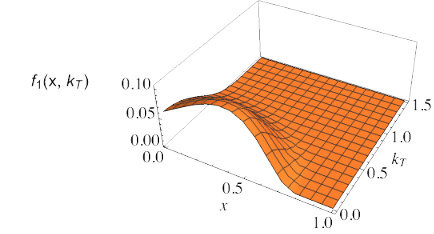
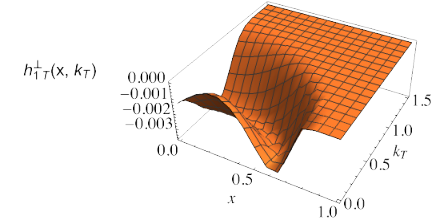
In figure 1 we show 3d plots of , , and for a bag radius of 0.8 fm and a recoil mass . Of particular note is that , and all peak at and are small for GeV, while shows interesting structure and a definite minimum at for . In contrast to the results of reference AESY10, we see that these distributions only have support on , and are normalizable on this interval so that no renormalization procedure is necessary to calculate moments or the Fourier transforms of these distributions. Also, these distributions are well-behaved as and go to zero in this limit, in accordance with the behaviour of given in equation (5).
Integrating our PDFs over the interval will yield sum rules, as shown in table 1. In this approach, the number and spin sum rules, calculated from and respectively, do not give the expected quark model values of and respectively. This occurs because only intermediate states with 2 quarks have been considered ST89; SST91, and other intermediate states such as and have not been added to the sum over all intermediate states. The tensor charge, given by the integral over the transversity PDF , is compatible with the recent determination of RB18, and will be investigated in further work.
We note that our TMDs automatically the satisfy the relation for the pretzelosity distribution AESY10
| (14) |
as the bag model obeys the conditions found in references LP11; LP12.
| 0.78 | 0.67 | 0.73 | 0.013 | 0.35 |
We find that the transverse momentum dependences of , and are well-fitted by Gaussian distributions of the form
| (15) |
with the Gaussian width showing some dependence, as would be expected from kinematic arguments CHS77; DS77.
In the bag model, flavour dependence is introduced through the colour hyperfine interaction. In this work we use an exact approach using hyperfine eigenfunctions, which raise the degeneracy of the masses of the singlet and triplet recoil states CT88; SST91. This has been criticised as being inconsistent with the Pauli exclusion principle Isgur99, however, careful consideration of the hyperfine eigenfunctions under normal assumptions about the spatial wavefunctions showed that the exclusion principle is not violated in this approach Signal17. An alternative is to use a perturbative approach involving mixing the SU(6) 56 nucleon wavefunction with higher mass 70 states. This approach will be examined in further work.
In figure 2 we plot the quark orbital angular momentum density, of the valence and quarks, calculated for a bag radius of 0.8 fm and the singlet - triplet recoil masses split by 100 MeV. In contrast to the usual parton distributions, are flat over the region and decrease in magnitude slowly at large , indicating that quark orbital angular momentum in the bag model is carried over a wide kinematic range, whereas at the bag model scale the spin dependent parton distributions are usually peaked in the valence region around and quickly become small at large . This behaviour arises because the orbital angular momentum only comes from the lower component of the relativistic quark wavefunction in equation (Transverse Momentum and Transverse Momentum Distributions in the MIT Bag Model), which is small at low momentum and increases to a maximum around , whereas the upper component decreases over this range of momenta. We find the valence quark orbital angular momenta are and , giving a total valence contribution of 0.016. This small orbital angular momentum may appear to contradict the picture of Myhrer and Thomas MT88; MT08; MT10, where the one-gluon exchange corrections to spin dependent quantities are dominated by diagrams involving the excitation of a -wave antiquark, and results in a large fraction of the proton spin being carried by orbital angular momentum. However, our calculation is for valence quarks, whereas the Myhrer and Thomas result is for the sum of quarks and antiquarks, with the antiquark diagrams giving the largest contribution. Extending our calculations to explicitly include antiquark contributions would give further insight into the role of orbital angular momentum in the make up of the proton spin. We note that is not gauge invariant, so this calculation is only applicable in the MIT bag model. However, the combination of orbital angular momentum and gluon spin is gauge invariant, and in the model , so this calculation does give us some insight into the portion of the proton’s spin that is not carried by quarks.
The -dependent moments of transverse momentum for a given TMD are given by
| (16) |
In figure 3 we plot both and for unpolarized valence and quarks, again calculated for fm and MeV. This calculation only takes into account 2-quark recoil states, and also ignores contributions from the nucleon’s pion cloud. While we see a difference between the and quarks, this is small, and compatible with the experimental observation that the Gaussian widths of TMDs are flavour independent Hermes13; Compass13. We find a marked dependence, in contrast to the results of AESY10, and large values of and at both low and medium . The average transverse momentum is larger than GeV for . At we find GeV2 for and respectively, compared with the values quoted for unpolarized quarks of GeV2 in the light-cone constituent model calculation of BEBS09 and GeV2 in AESY10. Our results are similar in magnitude to the calculation in the Nambu-Jona-Lasinio (NJL) model of MBCT12, however, in the NJL model calculation has only a moderate -dependence, and increases at large .
The TMDs have so far been calculated at a low momentum scale appropriate for the bag model SST91. In order to compare the calculated TMDs with experimental data on and we need to evolve these distributions up to experimental scales. Factorization of the TMDs Collins11 allows us to compare a non-singlet TMD at different scales and . Using equation (26) of reference AR11 we can write the ratio of the TMD at different scales
| (17) |
Here, the function is the collinear factor, which is independent of the scales and , and is calculated at some independent scale . The function is calculated perturbatively in QCD and holds for all , and the function describes the non-perturbative behaviour. We note the appearance of the energy cutoff scale used to regulate light-cone divergences, with AR11; Collins11. Also, this expression applies in the spatial transverse parameter () space, where is the Fourier transform of the TMD in momentum space
| (18) | |||||
where we have explicitly changed integration variable to the magnitude of recoil momentum. The ratio of non-peturbative factors only depends on the energy scales and a universal hadron independent function
| (19) |
where usually a quadratic form is used for , giving a Gaussian model description of the TMD. The perturbative function has been calculated to first order in AR11 and we use the NLO expression for . We can now take our TMD calculated in momentum space at bag scale , transform to space, evolve up to an experimental scale , and finally transform back to momentum space to obtain the evolved TMD to compare with data.
In figure 4 we show the unpolarized valence up and down TMDs () at for both the bag scale GeV and then evolved to GeV in both transverse momentum space and space. Here we have used GeV2, determined from a global fit LBNY03, , as usual, and have set , the approximate maximum impact parameter for the perturbative domain, to 0.5 GeV-1, although these calculations are not particularly sensitive to the value of .
We observe that at the initial scale the calculated become negative for larger than about 1.3 fm, which would appear to be incompatible with the interpretation of these distributions as probability distributions. However, it is worth noting that in QCD the positivity constraint on these distributions is only true in momentum space Collins11. Additionally, these distributions are not the same as the so-called impact parameter dependent quark distributions derived from Generalized Parton Distributions (GPDs) Burk00; Burk02. The impact parameter dependent distributions are defined in terms of the Fourier transform of a GPD , where is the momentum transfer between the non-forward hadron states. The Fourier conjugate variable to is denoted in Burk00; Burk02, and is interpreted as the perpendicular distance from the centre of momentum of the target hadron. This is not the same as the conjugate variable to , which we are using for TMDs. Here is the perpendicular distance from the path of the photon to the centre of the struck quark’s electric potential. If the two different impact parameters differ by a constant, then the shift theorem for Fourier transforms implies that the distributions will differ by a sinusoidal factor, and if one is positive definite, then the other is not guaranteed to always be positive. We hope to explore the relationship between TMDs and GPDs in further work.
Evolution of the distributions shifts them to smaller , and the tail of the distributions at fm becomes negligible. As expected, in momentum space evolution causes the distributions to broaden. For the evolved and distributions we find GeV2 respectively, which are compatible with the value of GeV2 found in STM10 using a Gaussian model with Hermes SIDIS data. In addition GeV respectively for the unpolarized valence and quarks, which are in reasonable agreement with determinations from EMC and Hermes data in CEGMMS06; EGMMP05, again derived using Gaussian models. We also investigated using the alternate parameters found by Konychev and Nadolsky KN06, who found a larger value of GeV-1 and also GeV2, GeV2 and . The evolution is most sensitive to the value of , and we find GeV2 for the valence and distributions, which are also compatible with the Hermes data.
The analysis of Anselmino et al. ABGMP14 gives over the complete range of the Hermes data, with data cuts GeV2 and , while their fits of the Compass data give with similar cuts. These values are somewhat dependent on the data cuts, and also on the use of the Gaussian ansatz; however, given the wide range in of both data sets, we would argue that our calculations are not incompatible with these analyses. We have seen that evolution of the TMDs increases their widths, so further evolution to higher can give agreement with these values of .
The procedure for evolution of the TMDs could be criticised on the basis that our starting scale GeV is not much greater than GeV, so the evolution equations based on LO and NLO expressions may not be reliable. However, in the case of DIS the evolution equations appear to work quite well down to these scales, where the NLO (and NNLO) corrections do not become too large, and evolution of PDFs from low scales below GeV2 can give good agreement with the experimental PDFs SST91; SMST92; CS03; GRV98. As NLO expressions for the perturbative functions applicable for the leading twist TMDs become available, it will be interesting to check the size of the corrections to LO evolution. We have also seen that the non-perturbative part of the evolution introduces uncertainties of the order of 5-10%, similar to the size of differences between LO and NLO PDFs. Additionally, we have only calculated twist-two contributions to the distributions, and ignored higher twist contributions, which may be present in the data and could complicate the comparison between our calculations and the data.
A related concern is that factorisation for TMDs requires Collins11, whereas our starting scale is similar to the size of we have calculated in the bag model. We do not know whether this has deeper implications for the evolution of our model TMDs, however, we have seen that the increase in as we have evolved is rather slow, which gives us some confidence that the corrections to our leading term are small.
In conclusion, we have extended earlier work using the MIT bag model to present new calculations of the twist two transverse momentum distributions in the model. These calculations have the correct support, and do not require any renormalization procedure. The distributions show strong -dependence of the average transverse momentum of valence quarks. We have seen that longitudinal and transverse momentum components of quark momenta should not be treated as independent in the scattering process, which has implications for the extraction of moments of the transverse momentum distributions, and for the understanding of experimental data on transverse quark momentum. Using factorisation, the calculated distributions can be evolved in to compare with experimental determinations of and . We found that our unpolarized valence distributions gave reasonably good agreement with the current data on transverse momentum coming from experiments.
In future work we will extend these calculations by including pion cloud contributions to the TMDs. This will enable us to investigate sea quark distributions as well as valence distributions, and to examine the transverse momentum dependence of the asymmetry, recently reported by the SeaQuest collaboration SeaQuest2021.


Acknowledgments
We are grateful to Peter Schweitzer and Tony Thomas for valuable discussions on aspects of this work and for helping to correct some errors in an earlier version of this letter.
References
- (1) J. C. Collins, Phys. Lett. B, 536 (2002), p. 44 https://doi.org/10.1016/S0370-2693(02)01819-1, https://arxiv.org/abs/hep-ph/0204004
- (2) A. Kotzinian, Nucl. Phys. B, 441 (1995), p. 234 https://doi.org/10.1016/0550-3213(95)00098-D, https://arxiv.org/abs/hep-ph/9412283
- (3) A. Airapetian et al. (Hermes Collaboration), Phys. Rev. D, 87 (2013), 074029 https://doi.org/10.1103/PhysRevD.87.074029, https://arxiv.org/abs/1212.5407.
- (4) C. Adolph et al. (Compass Collaboration), Eur. Phys. J., 73, (2013), p. 2531 https://doi.org/10.1140/epjc/s10052-013-2531-6, https://arxiv.org/abs/1305.7317
- (5) J. C. Collins, Nucl. Phys. B, 396 (1993) p. 161 https://doi.org/10.1016/0550-3213(93)90262-N, https://arxiv.org/abs/hep-ph/9208213
- (6) R. Seidl et al. (Belle collaboration), Phys. Rev. Lett., 96 (2006), 232002 https://doi.org/10.1103/PhysRevLett.96.232002, https://arxiv.org/abs/hep-ex/0507063
- (7) R. Seidl et al. (Belle collaboration), Phys. Rev. D, 99 (2019), 112006 https://doi.org/10.1103/PhysRevD.99.112006, https://arxiv.org/abs/1902.01552
- (8) H. Avakian, A. V. Efremov, P. Schweitzer and F. Yuan, Phys. Rev. D 81 (2010), 074035 https://doi.org/10.1103/PhysRevD.81.074035, https://arxiv.org/abs/1001.5467
- (9) B. Pasquini, S. Cazzaniga and S. Boffi, Phys. Rev. D, 78 (2008), 034025 https://doi.org/10.1103/PhysRevD.78.034025, https://arxiv.org/abs/0806.2298
- (10) J. She, J. Zhu and B-Q. Ma, Phys. Rev. D, 79 (2009), 054008 https://doi.org/10.1103/PhysRevD.79.054008, https://arxiv.org/abs/0902.3718
- (11) A. V. Efremov, P. Schweitzer, O. V. Teryaev and P. Zavada, Phys. Rev. D, 80 (2009) 014021 https://doi.org/10.1103/PhysRevD.80.014021, https://arxiv.org/abs/0903.3490
- (12) A. Bacchetta, F. Conti and M. Radici, Phys. Rev. D, 78, (2008) 074010 https://doi.org/10.1103/PhysRevD.78.074010, https://arxiv.org/abs/0807.0323
- (13) H H Matevosyan, W. Bentz, I. C. Cloët and A. W. Thomas, Phys. Rev. D, 85 (2012) 014021 https://doi.org/10.1103/PhysRevD.85.014021, https://arxiv.org/abs/1111.1740
- (14) M. Wakamatsu, Phys. Rev. D, 79 (2009) 094028 https://doi.org/10.1103/PhysRevD.79.094028, https://arxiv.org/abs/0903.1886
- (15) M. Burkardt, Phys. Rev. D, 62 (2000) 071503 https://doi.org/10.1103/PhysRevD.62.071503, https://arxiv.org/abs/hep-ph/0105324
- (16) M. Burkardt, Phys. Rev. D, 66 (2002) 114005 https://doi.org/10.1103/PhysRevD.66.114005, https://arxiv.org/abs/hep-ph/0209179
- (17) G. A. Miller, Phys. Rev. C, 76 (2007) 065209 https://doi.org/10.1103/PhysRevC.76.065209, https://arxiv.org/abs/0708.2297
- (18) S.Venkat, J. Arrington, G. A. Miller, and X Zhan, Phys. Rev. C, 83 (2011) 015203 https://doi.org/10.1103/PhysRevC.83.015203, https://arxiv.org/abs/1010.3629
- (19) F. Yuan, Phys. Lett. B, 575 (2003) p. 45 https://doi.org/10.1016/physletb.2003.09.052, https://arxiv.org/abs/hep-ph/0308157
- (20) H. Avakian, A. V. Efremov, P. Schweitzer and F. Yuan, Phys. Rev. D, 78 (2008) 114024 https://doi.org/10.1103/PhysRevD.78.114024, https://arxiv.org/abs/0805.3355
- (21) A. I. Signal and A. W. Thomas, Phys. Rev. D, 40 (1989) p. 2832 https://doi.org/10.1103/PhysRevD.40.2832
- (22) A. W. Schreiber, A. I. Signal and A. W. Thomas, Phys. Rev. D, 44 (1991) p. 2653 https://doi.org/10.1103/PhysRevD.44.2653
- (23) A. W. Schreiber, P. J. Mulders, A. I. Signal and A. W. Thomas, Phys. Rev. D, 45 (1992) p. 3069 https://doi.org/10.1103/PhysRevD.45.3069
- (24) W. Greiner, S. Schramm and E. Stein, Quantum Chromodynamics, Third Edition, Springer-Verlag, Berlin (2007).
- (25) G. P. Lepage and S. J. Brodsky, Phys. Rev. D, 22 (1980) p. 2157 https://doi.org/10.1103/PhysRevD.22.2157
- (26) H-C, Pauli and S. J. Brodsky Phys. Rev. D, 32 (1985) p. 1993 https://doi.org/10.1103/PhysRevD.32.1993
- (27) J. C. Collins, Foundations of Perturbative QCD, Cambridge University Press, Cambridge (2011).
- (28) A. I. Signal, Nucl. Phys. B., 497 (1997) p. 415 https://doi.org/10.1016/S0550-3213(97)00231-9, https://arxiv.org/abs/hep-ph/9610480
- (29) R. E. Peierls and J. Yoccoz, Proc. Phys. Soc, A70, (1957) p. 381
- (30) C. Lorcé and B. Pasquini, Phys. Rev. D, 84 (2011) 034039 https://doi.org/10.1103/PhysRevD.84.034039, https://arxiv.org/abs/1104.5651
- (31) C. Lorcé and B. Pasquini, Phys. Lett. B, 710 (2012) p. 486 https://doi.org/10.1016/j.physletb.2012.03.025, https://arxiv.org/abs/1111.6069
- (32) M. Radici and A Bacchetta, Phys. Rev. Lett. 120 (2018) 192001 https://doi.org/10.1103/PhysRevLett.120.192001, https://arxiv.org/abs/1802.05212
- (33) F. E. Close, F. Halzen and D. M. Scott, Phys. Lett. B, 68 (1977) p. 447 https://doi.org/10.1016/0370-2693(77)90466-X
- (34) A. C. Davis and E. J. Squires, Phys. Lett. B, 69 (1977) p. 249 https://doi.org/10.1016/0370-2693(77)90655-4
- (35) F. Myhrer and A. W. Thomas,Phys. Rev. D, 38 (1988) 1633 https://doi.org/10.1103/PhysRevD.38.1633
- (36) F. Myhrer and A. W. Thomas, Phys. Lett. B, 663 (2008) p. 302 https://doi.org/10.1016/j.physletb.2008.04.034, https://arxiv.org/abs/0709.4067
- (37) F. Myhrer and A. W. Thomas, J. Phys. G, 37 (2010) 023101 http://doi.org/10.1088/0954-3899/37/2/023101, https://arxiv.org/abs/0911.1974
- (38) M. Anselmino, M. Boglione, J. O. Gonzalez H, S. Melis and A. Prokudin, JHEP, 04 (2014) 005 https://doi.org/10.1007/JHEP04(2014)005 https://arxiv.org/abs/1312.62617a
- (39) F. E. Close and A. W. Thomas, Phys. Lett. B, 212 (1988) p. 227 https://doi.org/10.1016/0370-2693(88)90530-8
- (40) N. Isgur, Phys. Rev. D, 59 (1999) 034013 https://doi.org/10.1103/PhysRevD.59.034013, https://arxiv.org/abs/hep-ph/9809255
- (41) A. I. Signal, Phys. Rev. D, 95 (2017) 114010 https://doi.org/10.1103/PhysRevD.95.114010, https://arxiv.org/abs/1702.05152
- (42) S. Boffi, A. V. Efremov, B. Pasquini and P. Schweitzer, Phys. Rev. D, 79 (2009) 094012 [https://doi.org/10.1103/PhysRevD.79.094012, https://arxiv.org/abs/0903.1271].
- (43) S. M. Aybat and T. C. Rogers, Phys. Rev. D, 83 (2011) 114042 https://doi.org/10.1103/PhysRevD.83.114042, https://arxiv.org/abs/1101.5057
- (44) F. Landry, R. Brock, P. M. Nadolsky and C. P. Yuan, Phys. Rev. D, 67 (2003) 073016 https://doi.org/10.1103/PhysRevD.67.073016, https://arxiv.org/abs/hep-ph/0212159
- (45) P. Schweitzer, T. Teckentrup, and A. Metz, Phys. Rev. D, 81 (2010) 094019 https://doi.org/10.1103/PhysRevD.81.094019, https://arxiv.org/abs/1003.2190
- (46) J. C. Collins, A. V. Efremov, K. Goeke, S. Menzel, A. Metz and P. Schweitzer, Phys. Rev. D, 73 (2006) 014021 https://doi.org/10.1103/PhysRevD.73.014021, https://arxiv.org/abs/hep-ph/0509076
- (47) J. C. Collins et al. Phys. Rev. D, 73 (2006) 094023 https://doi.org/10.1103/PhysRevD.73.094023, https://arxiv.org/abs/hep-ph/0511272
- (48) A. V. Efremov, K. Goeke, S. Menzel, A. Metz and P. Schweitzer, Phys. Lett. B, 612 (2005) 233 https://doi.org/10.1016/j.physletb.2005.03.010, https://arxiv.org/abs/hep-ph/0412353
- (49) A. V. Konychev and P, M. Nadolsky, Phys. Lett. B, 633 (2006) 710 https://doi.org/10.1016/j.physletb.2005.12.063, https://arxiv.org/abs/hep-ph/0506225
- (50) F. G. Cao and A. I. Signal, Phys. Rev. D, 68 (2003) 074002 https://doi.org/10.1103/PhysRevD.68.074002, https://arxiv.org/abs/hep-ph/0306033
- (51) M. Glück, E. Reya and A. Vogt Eur. Phys. J., 5 (1998) p. 461 https://doi.org/10.1007/s100529800978, https://arxiv.org/abs/hep-ph/9806404
- (52) J. Dove et al. (SeaQuest collaboration), Nature, 590 (2021) p. 561 https://doi.org/10.1038/s41586-021-03282-z, https://arxiv.org/abs/2103.04024