TIT/HEP-686 August 2021 Finite- superconformal index via the AdS/CFT correspondence
We propose a prescription to calculate the superconformal index of the supersymmetric Yang-Mills theory with finite on the AdS side. The finite corrections are included as contributions of D3-branes wrapped around three-cycles in , which are calculated as the index of the gauge theories realized on the wrapped branes. The single-wrapping contribution has been studied in a previous work, and we further confirm that the inclusion of multiple-wrapping contributions correctly reproduces the higher order terms as far as we have checked numerically.
1 Introduction
The AdS/CFT correspondence [1] has been intensively investigated in the large limit, and agreement of many quantities calculated on the both side of the duality has been confirmed. Although the quantum gravitational effect becomes important for finite , it may be possible to calculate some quantities associated with topology and supersymmetry on the AdS side. Let us consider the duality between 4d SYM and the string theory in . The relation among the AdS radius , the ten-dimensional Planck length , and the D3-brane tension suggests that when is finite not only the quantum gravitational effect but also the contribution of D3-branes extended in becomes important, and the finite corrections for some quantities may be reproduced as the contribution of D3-branes. One such example is the BPS partition function of SYM. It was calculated by the geometric quantization of BPS D3-brane configurations (sphere giants [2, 3]) in [4]. (See also [5] for another derivation using AdS giants [6, 7].) In this paper we discuss a similar calculation of the superconformal index [8] for finite on the AdS side.
The basic idea is as follows. We start from the large limit, in which the index is reproduced as the supergravity contribution in the holographic dual description [8]. We include finite corrections as contributions of branes wrapped around topologically-trivial three-cycles in the internal space . The analysis of single-wrapping contributions has been already done in [9], and it was confirmed that finite corrections are correctly reproduced up to errors which can be interpreted as the multiple-wrapping contributions. The multiple-wrapping contributions were calculated in [10] for the Schur index [11] of 4d SYM, and the analytic result of [12] was successfully reproduced. In this paper we improve the calculation in [10], and confirm that we can also calculate the superconformal index in a similar way.
In terms of multiplets the theory consists of a vector multiplet and three adjoint chiral multiplets (). The superconformal index is defined by
| (1) |
We use the Hamiltonian , left- and right-handed spins and , and R-charges as the Cartan generators of the superconformal algebra . acts on the corresponding chiral field with charge . 11 1 We use unusual normalization of R-charges such that carries . The supercharge associated with the index (1) carries the following quantum numbers:
| (2) |
The formula we use to calculate the index has the following form:
| (3) |
where is the supergravity contribution giving the large index and the sum over gives the finite corrections arising from wrapped D3-branes. are the numbers of D3-branes wrapped on three-cycles labeled by . Let be the three complex coordinates corresponding to . The internal space is given by . Each of generates phase rotation of the corresponding -plane. Three three-cycles () are defined by . For a set of the wrapping numbers , the gauge theory realized on the wrapped D3-branes is the gauge theory with three bi-fundamental hypermultiplets shown as the quiver diagram in Figure 1.

This looks like the toric diagram of . This is not accidental but holds for general toric quiver gauge theories [13]. is the index of the D-brane system specified by the wrapping numbers and .
To sort out the results of our calculation it is convenient to define the total wrapping number
| (4) |
The contribution from each is of order where are non-negative integers. In the large limit the sectors with decouples and only the sector contributes to the index. Then (3) reduces to , which was confirmed in [8].
The contribution of the sector was investigated in [9]. In this case the theory on the wrapped D3-brane is a supersymmetric gauge theory consisting of only neutral fields, and we can easily calculate without any holonomy integrals. It was found that (3) reproduces the correct index up to expected error due to multiple-wrapping contribution of order with .
The purpose of this paper is to study the contributions from . There are two issues we have to settle for the purpose. One is about the gauge fugacity integrals. If , the theory on wrapped D3-branes is a gauge theory with charged fields. We can write down the contribution in the matrix integral form just like standard localization formulas. In order to carry out the gauge fugacity integrals we need to carefully specify the integration contours, because due to a reason we will explain in Section 3 we cannot use the standard choice, the unit circle on the complex plane of the gauge fugacities. The other is related to a global symmetry of the quiver gauge theory of Figure 1. A gauge invariant operator of this theory can be associated with a closed path in the quiver diagram. If all are positive, there exist operators corresponding to paths going around the triangle. Let be the global symmetry coupling to such operators. Because there is no corresponding symmetry in the boundary SYM, the fugacity variable cannot be an independent variable but it must be given as a function of other fugacities. We have to fix these two ambiguities, one for integration contours and the other for . We will propose how to fix these and confirm it gives the correct index.
This paper is organized as follows. In the next section we gives a detailed description of the formula (3) except for the ambiguities mentioned above. In Section 3 we propose a basic rule to determine the integration contours. In fact, the ambiguity for the integration contours is not fixed only by the rule in Section 3. The ambiguities concerning the contours and are fixed in section 4 by using “the pole cancellation condition,” which requires the index does not diverge in the unrefined limit . We also numerically confirm in Section 4 that the prescription reproduces the correct finite index up to very high order of . The final section will be devoted to summary and discussion.
2 Formula
In this section we give a detailed explanation of the formula (3). The basic idea was first given in [9].
In the large limit it is well known that the index is reproduced on the AdS side as the supergravity index [8]. is the plethystic exponential defined in the next section. is the single-particle index
| (5) |
The finite corrections in (3) are given by
| (6) |
is the classical factor coming from the classical charges and energy of the wrapped brane system. Its explicit form is
| (7) |
and this is the only place in the formula where the rank appears. are the integration measures associated with gauge group.
| (8) |
() are gauge fugacities of .
The integrand consists of two factors. “(vector)” is the contribution from the vector multiplets and given by
| (9) |
where are the single-particle indices of vector multiplets. is given by
| (10) |
and are obtained by permutations among .
The hypermultiplet contribution “(hyper)” is
| (11) |
where is treated as a cyclic variable and when means . Three variables , , and are (redundant) fugacities, and the integral depends only on their product . If some of are zero, we can absorb these degrees of freedom by a redefinition of gauge fugacities and we can neglect them. In the boundary gauge theory there is no parameter corresponding to , and the associated symmetry should be broken. This means is not an independent variable but a function of other fugacities. are the single-particle indices of hypermultiplets. is given by
| (12) |
and are obtained from this by the permutations. For derivations of (10) and (12) see Appendix A.
3 Pole selection rule
The contribution of a single D3-brane wrapping around a cycle is given by . The plethystic exponential is defined as follows. The -expansion of in general has the form
| (13) |
where the first sum and the second sum are bosonic and fermionic contributions, respectively. Each term or gives a quantum of a harmonic oscillator. Summing up the contribution from all states of the oscillator we obtain
| (14) |
for a bosonic oscillator and
| (15) |
for a fermionic oscillator. The plethystic exponential is defined by these two relations and the addition formula representing the decoupling among oscillators.
An unusual point in the calculation of the wrapped D-brane contribution is the existence of tachyonic modes, which have negative energies. Such modes correspond to terms in with negative power of . The existence of such modes are related to the fact that the cycle is topologically trivial. Usually we take and other fugacities to be phases, and if there exists such tachyonic modes the geometric series in (14) does not converge. In [9] it was proposed that when the geometric series (14) diverges we should define the plethystic exponential by analytically continued form:
| (16) |
Namely, we define the plethystic exponential of (13) by
| (17) |
As far as we have checked this trick works quite well and correct indices are reproduced in many cases. If includes negative power of the -expansion of its plethystic exponential around starts at positive power of . This is the origin of the tachyonic shift for .
In the case of , the gauge group realized on the wrapped brane system is or . Because the diagonal always decouples we have one non-trivial gauge integral. It typically has the form
| (18) |
where is a -series of the form (13). The integrand has poles at and for each , and these two poles have opposite residues. Let us call these two series of poles “positive poles” and “negative poles”, respectively. The problem is which poles we should pick up in the integral (18).
If we consider case the situation becomes more complicated. We need to consider the multiple integrals. Let be the gauge fugacities, and let us carry out the integrals in this order. Because all fields belong to the adjoint or bi-fundamental representations, we can set the last one to be one. Let us consider the -th integral (). The gauge fugacity appears in the single-particle index in the form or . These produce the poles at and , respectively. If , the integral has not yet been performed at the moment of the integral, and we treat the former and the latter as a positive pole and a negative pole, respectively. However, if , has been replaced with the position of a pole on the plane by the integral. By taking account of this, the position of a pole on the plane in general has the following form
| (19) |
where . There are three types of poles
- •
, : positive poles
- •
, : negative poles
- •
, : mixed poles
Which poles should we pick up in the -integral? In the usual situation with and the unit circle as the integration contour, the contour encloses all positive poles (and ). Naively, the contour seems to enclose a part of mixed poles. In fact, however, we can show that the mixed poles do not appear due to a certain cancellation (See Appendix B). Therefore, in the standard situation with , using the unit circles is equivalent to taking only positive poles at each step of integrals.
Our proposal is to keep using this prescription regardless of being inside or outside of the unit circle.
- The pole selection rule
-
In the case with the wrapping number , we have gauge fugacities (). Let us suppose that we carry out the integral in the order . Because the last -integral is trivial, we can set and we have only non-trivial integrals. In the -integral at the -th step () we have the following two types of poles other than :
(20) where the former and the latter are associated with terms and in the single-particle index, respectively. The rule we propose is to include poles at and and exclude ones at . When we choose a pole with we substitute to the pole position chosen in the preceding -integral.
This rule does not refer to the numerical values of , and gives the index as an analytic function of .
The analysis in [10] of the Schur index supports this rule. The Schur index is defined from the superconformal index by taking the limit [11]. In this limit the index becomes a function of only two fugacities and , and the pole structure in the gauge fugacity integrals is much simpler than that of the superconformal index. In [10] it was found that if we pick up positive poles at each step of the gauge fugacity integrals the correct Schur index is reproduced.
4 Comparison
We can calculate the index unambiguously on the gauge theory side by using the localization formula. The results for are
| (21) |
(We set and leave only to save the space. We use the notation “” to represent this unrefined limit.) We want to reproduce these on the gravity side.
4.1
Let us compare these with the supergravity contribution . The -expansion of is
| (22) |
Let be the finite correction. For small it is given by
| (23) |
The leading term of each correction is of order . We want to reproduce these corrections by wrapped D3-branes on the AdS side.
4.2
The contribution was investigated in [9]. For the index (6) reduces to
| (24) |
By using the prescription for the tachyonic mode this gives
| (25) |
The other two single-wrapping contributions from and are obtained in a similar way. The total contribution from is
| (26) |
and for it is given by
| (27) |
These correctly reproduces many terms appearing in (23).
Although we only show the results in the unrefined limit in (27), we cannot set before summing up the three contributions in (26). As is seen in (25) each of has the pole at . The most singular part in the expansion in the leading term of the -expansion is
| (28) |
and diverges at . The poles in cancel only after three contributions are summed in (26). This pole cancellation plays an important role when we discuss contributions.
Even after taking account of the single-wrapping contributions, we still have the error
| (29) |
For the remaining errors are as follows.
| (30) |
The leading term for each is of order . Our next task is to reproduce these corrections as double-wrapping contributions.
4.3
There are six configurations with total wrapping number .
| (31) |
Each of the first three terms is contribution of two D3-branes wrapping on the same cycle, on which gauge theory is realized. The Cartan part simply gives the square of the single-wrapping contribution. In addition we need to include the W-boson contribution. For example, is given by
| (32) |
with the W-boson contribution
| (33) |
Let us look at the pole structure of the integrand. The -expansion of is
| (34) |
Let () be the positive terms in the expansion. There are one tachyonic term and two zero-mode terms.
| (35) |
In addition, we have infinite number of () with positive exponent of . According to the rule we take the contour enclosing all positive poles (Figure 2).

The result of the contour integral is22 2 In the practical calculation we need to introduce a cut-off in the -expansion of the single-particle index. For a detailed explanation about the cut-off order see Appendix C.
| (36) |
Just like the single wrapping contributions, has a pole at , which comes from both and . The most singular part in the leading term of is
| (37) |
Notice that this pole does not cancel even in the sum . This should be cancelled by the other three contributions including the hypermultiplets.
Each of the last three terms in (31) is the contribution of two D3-branes wrapping on two different cycles. The gauge group on the branes is and fields on each brane are neutral. Therefore, the contribution from the vector multiplets is simply the product of single-wrapping contributions for two branes. The extra contribution we need to calculate is the hypermultiplet arising from open strings stretched between two D3-branes. For example, is given by
| (38) |
with the hypermultiplet contribution
| (39) |
Let us look at the pole structure of the integrand.
The -expansion of the hypermultiplet single-particle index (12) is given by
| (40) |
where , , , and are positions of poles , and zeros , of the integrand. They are given by
| (41) |
and satisfy the relations
| (42) |
The plethystic exponential of is given by
| (43) |
where the function is defined by 33 3 In the Schur limit the zeros and poles of the integrand of the hypermultiplet contribution (39) collide: , , and the elliptic function becomes trivial: .
| (44) |
This function satisfies
| (45) |
Let us define and by and , respectively. If we regard as the function of , is an elliptic function with periods and , and satisfies . The position of poles on the -plane are and . They appear on the -plane as two poles in the fundamental region. (Figure 3)

Due to (45) all residues are the same up to the signs:
| (46) |
Now, let us calculate the contour integral. The positive poles read off from the single-particle index (40) are
| (47) |
The contour on the -plane enclosing poles in (47) and is the cycle in the torus shown in Figure 3. The contour integral gives
| (48) |
Using this, we obtain with the most singular part
| (49) |
Disappointingly, (49) does not cancel the pole at of (37). This means that we need to choose another contour. Because all residues are the same up to sign, we can change the integral by only a multiple of the residue (46). Fortunately, we can find a contour with which the pole cancellation works. If we exclude one pole at and use the contour in Figure 3, the integral becomes
| (50) |
The most singular part of becomes
| (51) |
and this successfully cancel not only most singular part shown in (51) but also all other divergences.
How should we treat the adoption of the contour , which is different from determined by the pole selection rule? It is important that the presence of two kings of poles, positive and negative ones, is related not to the function itself but to the single-particle index. There may be the case that two different single-particle indices give the same plethystic exponential up to unimportant factors, and then the definition of the positive and negative poles may depend on which single-particle index is adopted. In fact, we can find a single-particle index with which the pole selection rule gives the desired contour . We can rewrite (11) as
| (52) |
where and we defined the modified single-particle index
| (53) |
We can show that (52) is the same as (11) by using the relation
| (54) |
Therefore, this does not affect the integrand in (6). However, the difference of the single-particle indices affects the definition of the positive and negative poles, and the rule with gives the contour . With the modified single-particle index we can keep the pole selection rule intact. We will use the modified single-particle index for all calculations in the following.
Finally, let us compare (31) and (30). The total double-wrapping contribution (31) for small calculated with the pole selection rule described above are as follows:
| (55) |
These agree with many terms appearing in (30).
The error terms are expected to be of order . However, it is difficult to explicitly calculate them for due to the limited computational resources. Not only the physical range , we can also use unphysical values and for consistency check. is the trivial theory with and is the empty theory with . For , the errors are given by
| (56) |
and the leading terms are of order as expected.
4.4
At there are brane configurations.
| (57) |
For of them we can calculate the contour integral with the omission of . With the pole selection rule, is given by
and and are obtained by the permutations among . To calculate we use the pole selection rule with the modified hypermultiplet single-particle index. The result is
and other five contributions are obtained by the permutations among . We need a special care about . In this case the quiver diagram has a loop, and we cannot simply neglect the fugacities . Unlike the other nine contributions does not have term and starts at :
| (66) |
where .
Concerning terms, the poles at successfully cancel among the nine contributions. For the higher order terms we need to include , which depends on . If we require the cancellation among poles at we need to set44 4 Although we introduced three fugacities , , and to make the cyclic symmetry manifest, the results depends only on the product , and we can practically set .
| (67) |
The result up to the order we have calculated is symmetric under and we cannot choose one of and .
4.5
For the computational cost rapidly increases and we can say only little about these contributions due to the limited computational resources. At there are four essentially different contributions: , , , and , and other contributions are obtained from these by simple permutations among . We obtained the leading terms of some of them, which is of order . From these results and the results for we can guess the general form of the term in as follows:
| (69) |
where are the following polynomials of .
| (70) |
By definition monomials of are associated with the points in the weight lattice, and with this relation the terms in form a triangle in the lattice (Figure 4).

If all are non-zero (69) vanishes.
Although we have not yet confirmed that (69) reproduces the correct index of the gauge theory, it is easy to check that it satisfies the pole cancellation condition for different values of , and sums up to
| (71) |
5 Summary and Discussion
We proposed a prescription to calculate the superconformal index of SYM up to an arbitrary order of the -expansion based on the idea of [9] and the prescription for the Schur index in [10]. We fixed the selection rule for poles associated with hypermultiplets and fugacity so that the poles at cancel, and confirmed that the index obtained with the prescription agrees with the correct one as far as we have checked numerically.
Our formula (3) is based on some assumptions, and at this moment we do not have any proof. It is desirable to check whether it works for . This requires effective method to carry out the contour integrals. It would be also important to test our prescription in other systems than the SYM. The single-wrapping contributions were analyzed for 4d orbifold quiver gauge theories [14], 4d toric quiver gauge theories [13], 6d theories [15], and 6d theories [16]. In [15] multiple-wrapping contributions to the 6d Schur-like index were partially calculated and the agreement with the results in [17, 18] was found. More detailed analysis of these and other systems including multiple wrapping contributions are desired.
It was recently found that the superconformal index has the information about the entropy of the AdS blackhole [19]. In general, in the statistical derivation of thermodynamic quantities we first calculate the partition function , where is energy levels, is the degeneracies of each level, and is the damping factor of the canonical ansamble. In the thermodynamic situation we can regard as a smooth function of the energy , and the summand of the partition function has a sharp peak at (Figure 5). From the summand and the coefficient at the peak we can determine the free energy and the entropy .
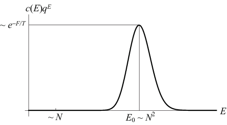
The analysis in [19] revealed that even if we replace the partition function by the superconformal index, we can still obtain the entropy by tuning fugacity variables appropriately. When we discuss macroscopic black hole we usually consider parameter region with , while the focus in this paper is the region . It is important to clarify how these two regions are interpolated. If our prescription works for arbitrarily large , it may be possible to reproduce the blackhole entropy on the AdS side without using the quantum gravity.
Acknowledgments
The author would like to thank S. Fujiwara for providing some results of numerical analysis in Section 4. The author also thank R. Arai for collaboration at the early stage of this work. The work of Y. I. was partially supported by Grand-in-Aid for Scientific Research (C) (No.21K03569), Ministry of Education, Science and Culture, Japan. This work used computational resources TSUBAME3.0 supercomputer provided by Tokyo Institute of Technology.
Appendix A Single-particle indices
A.1 Modes on a wrapped D3-brane
The single particle indices were first derived in [9] by using the automorphism between the supersymmetry algebra on the boundary and that on the wrapped D3-brane. In this appendix we derive the same result more directly.
A half of the supersymmetries is broken by the introduction of a wrapped D3-brane and modes on the D3-brane form a representation of the preserved algebra. Let us start with specifying this algebra.
We express as the subset of defined by where are three complex coordinates in . We define three Cartan generators , , and acting on three complex coordinates. We introduce a D3-brane wrapped on the large defined by , and this breaks acting on to , where the Cartans of the two factors are
| (72) |
The supercharges , , , and belong to quartet (the fundamental or the anti-fundamental) representations of . Each of them is decomposed into a pair of doublets of the unbroken symmetry . The one from each pair satisfying is preserved by the D3-brane and the other is broken. The preserved supersymmetries are summarized in Table 1.
is the generator of the outer automorphism of rotating the supercharges by . Note that the preserved components of and anti-commute among them, and the algebra does not include the and generators. The algebra generated by these supercharges is the product of two isomorphic algebras , which are generated by the following generators:55 5 and
| (73) |
and are central elements and they are both identified with .
Important anti-commutation relations for the construction of representations are
| (74) |
Other anti-commutation relations among supercharges vanish. From these we obtain the bounds
| (75) |
Next, let us consider component fields of the vector multiplet on the D3-brane. A vector multiplet consists of five component fields distinguished by (Figure 6 (a)). On a flat D3-brane in the flat spacetime they belong to representations of the R-symmetry . We emphasize that is different from the R-symmetry of the boundary theory acting on . acts on the six transverse directions of the wrapped D3: four in and two in . Due to the curvature of the background spacetime is broken to . The two factors are identified with the spins in AdS. The component fields are decomposed into nine irreducible representations of this subgroup as in Figure 6 (b).

We can determine the Kaluza-Klein spectrum without using the detailed information of the theory (equations of motion of the fields) thanks to the large symmetry. In general, we can construct an irreducible representation by acting and as raising operators on primary states. Because both and carry we can use as “the level” in the construction. The fields on the D3-brane carry different values on as is shown in Figure 6 (b), and carries the smallest value . The scalar field is expanded into spherical harmonics belonging to the representation
| (76) |
Let be the set of modes belonging to . For each we can construct an irreducible representation of by acting the raising operators and repeatedly on .
The diagram in Figure 6 (b) shows that and eliminate and the representation must be short for both and . Hence the highest weight state in the harmonics should saturate both the bounds in (75). This determines the common central charge as
| (77) |
Now we have completely determined the quantum numbers of modes of . See the line of in Table 2.
The full representation of is constructed by acting and on the primary states and removing zero norm states. Because the algebra is factorized, we can consider excitations of and ones of separately. Let us focus on the part. The quantum numbers of for the bosonic subalgebra
| (78) |
are . By acting and removing null states we obtain the irreducible representation
| (79) |
A spin representation with negative should be removed. Namely, for and the representations are
| (80) |
We can also construct the representation as a direct sum of irreducible representations of the bosonic subgroup , which are given in the same way as (79) and (80). The modes on a wrapped D3-brane belong to the representation
| (81) |
All modes belonging to (81) are summarized in Table 2. Using the information in the table it is straightforward to obtain the single-particle index
| (82) |
Some comments are in order.
The mode of , the unique component of the representation has negative energy. This does not contradict the supersymmetry because always appears in the unbroken algebra in the form , and itself is not subject to any bounds.
The modes are Nambu-Goldstone modes associated with the symmetry breaking. The broken generators are realized non-linearly on the D3-brane and behave like creation and annihilation operators. modes are generated by broken generators, and the quantum numbers agree with those of the corresponding generators. Modes in have and generate degenerate states belonging to the representations. A mode in or saturate the BPS bound associated with the broken supercharge which carries the same quantum numbers with the mode. The bose-fermi pairing caused by such a mode is the reason for the vanishing of the index in a special limit like the Schur limit.
A.2 Modes on the intersection
We consider two wrapped D3-branes: one wrapped on and the other wrapped on . The supercharges with are preserved. The quantum numbers of unbroken supersymmetry generators are summarized in Table 3.
The non-vanishing anti-commutation relations among the preserved supercharges are
| (83) |
Again, the preserved superconformal algebra factorizes to two isomorphic algebras generated by the following generators:
| (84) |
From (83) we obtain the bounds
| (85) |
A single hypermultiplet lives on the intersection locus of the two D3-branes. It consists of a chiral multiplet arising from open strings of one orientation and another chiral multiplet from open strings of the opposite orientation. The two chiral multiplets carry opposite gauge charges and the other quantum numbers are the same. Let us focus on one of these chiral multiplets. It includes two bosonic and two fermionic degrees of freedom.
In the case of the flat spacetime background scalar fields belong to a doublet of the rotation of the four DN directions and fermion fields are singlet under the . This is not affected by the background curvature. Namely, we have two bosonic components with and fermionic components with .
The charge is the Kaluza-Klein momentum along the intersection. Because of the non-vanishing of the supercharges the bosonic and fermionic components satisfy different quantization condition of . Namely we should consider the NS-sector, and for bosonic components and for fermionic components. We expand , , and into Fourier modes , , and , respectively, where and denote the Kaluza-Klein momentum . By requiring all modes to belong to short superconformal representations the energy of all modes are determined as shown in Table 4.
The BPS bounds in (85) show that if scalar modes and are singlets and if they are singlets. With this information we can unambiguously determine the multiplet structure as shown in Figure 7.

From the quantum numbers in Table 4 we can easily calculate the single particle index:
| (86) |
Appendix B Mixed poles
After repeating the integrals we may have the following factor in the integrand at the step of -integral.
| (87) |
Then, we have a mixed pole at
| (88) |
Although this pole may sit inside the unit circle, the above pole selection rule does not include mixed poles like this. In fact, this kind of poles always cancel among them, and in total do not contribute to the result. Let us prove this by mathematical induction.
Let us consider poles on the -plane after the integrals with respect to variables
| (89) |
We suppose that at every step of these integrals mixed poles cancel among them, and based on this assumption we want to show that this is also the case for the -integral.
Let us first consider how the factor (87) is generated by the preceding integrals. Due to the assumption that mixed poles cancel in the first integrals, (87) should be generated from a factor
| (90) |
by the substitusions
| (91) |
The first substitution in (91) is realized if the integrand contain
| (92) |
and picking up positive poles in the integrals with respect to variables
| (93) |
The order of the variables in (93) has nothing to do with the integration order. Similarly, the second in (91) is realized if the integrand contains
| (94) |
and picking up positive poles from these factors in the integrals with respect to variables
| (95) |
Let be the product of all factors in (90), (92), and (94), and be the remaining factor in the integrand. Namely, the integrand before starting the integrals is . After performing integrals for variables (89) by picking up the poles we described above we obtain
| (96) |
where and are the values substituted to and , respectively, after the integrals with respect to the variables in (89). If (89) contains variables that are not contained in either (93) or (95), in (96) should be understood as the function obtained by the integrals with respect to them. Now let us perform the -integral around the mixed pole (88). The result is
| (97) |
What we want to show is there is always another contribution that cancels this result.
Notice that every integration variable in (93) or (95) appears in twice. Except for , each of them appears once in a numerator and once in a denominator. Unlike the other variables appears twice in denominators in the two factors, the seed factor (90) and the first factor in (94). Corresponding to these two factors there are two positive poles
| (98) |
on the -plane. In the calculation above we took the latter in (98) in the -integral.
Now, let us exchange the roles of the two poles in (98). Namely, we pick up the formar in the -integral. Then, as the result of integrals with respect to the variables in (89), we obtain the following factor:
| (99) |
instead of (96). and in (99) are the same as those in (96). This is similar to (96), and produces the pole at the same position (88). Furthermore, we can easily confirm that the -integral around the pole (88) gives the negative of (97), and the two contributions calcel each other. In this way, all mixed poles cancel among them and we only need to take account of positive poles as is claimed in the pole selection rule.
Appendix C Cut-off order
The -expansion of the single-particle index includes infinite terms and in a practical numerical calculation we need to introduce cut-off at some order. To obtain correct results up to desired order we need to choose the cut-off order carefully. To determine the appropriate order of the cut-off let us consider the effect of the inclusion of a term of order to the single-particle index.
Let be the order of the leading term in the -expansion of the final result. The inclusion of an term into the single-particle index produces the extra factor
| (100) |
in the integrand. If we used the unit circle in the every -integral, this would change the integral by the factor , and the correction to the final result would be of order . However, we need to consider the case with tachyonic terms in the single-particle index. Let us assume that the leading term of the expansion of the single-particle index starts at order . If we cannot use unit circles for the contours. We need to deform the contours to include all positive poles and exclude all negative poles. In the rank case we need to perform the integrals times, and the final -integral, the most distant positive pole from the origin is , while the closest negative pole to the origin is . Therefore, varies on the contour in the following range:
| (101) |
As the result, the factor (100) becomes
| (102) |
Therefore, the inclusion of term in the single-particle index affect the result by terms of order . Contrary, if we want to obtain the correct answer up to terms, then it is sufficient if we include terms up to in the single-particle index, where
| (103) |
References
- [1] J. M. Maldacena, “The Large N limit of superconformal field theories and supergravity,” Int. J. Theor. Phys. 38, 1113 (1999) [Adv. Theor. Math. Phys. 2, 231 (1998)] doi:10.1023/A:1026654312961, 10.4310/ATMP.1998.v2.n2.a1 [hep-th/9711200].
- [2] J. McGreevy, L. Susskind and N. Toumbas, “Invasion of the giant gravitons from Anti-de Sitter space,” JHEP 0006, 008 (2000) doi:10.1088/1126-6708/2000/06/008 [hep-th/0003075].
- [3] A. Mikhailov, “Giant gravitons from holomorphic surfaces,” JHEP 0011, 027 (2000) doi:10.1088/1126-6708/2000/11/027 [hep-th/0010206].
- [4] I. Biswas, D. Gaiotto, S. Lahiri and S. Minwalla, “Supersymmetric states of N=4 Yang-Mills from giant gravitons,” JHEP 0712, 006 (2007) doi:10.1088/1126-6708/2007/12/006 [hep-th/0606087].
- [5] G. Mandal and N. V. Suryanarayana, “Counting 1/8-BPS dual-giants,” JHEP 0703, 031 (2007) doi:10.1088/1126-6708/2007/03/031 [hep-th/0606088].
- [6] M. T. Grisaru, R. C. Myers and O. Tafjord, “SUSY and goliath,” JHEP 0008, 040 (2000) doi:10.1088/1126-6708/2000/08/040 [hep-th/0008015].
- [7] A. Hashimoto, S. Hirano and N. Itzhaki, “Large branes in AdS and their field theory dual,” JHEP 0008, 051 (2000) doi:10.1088/1126-6708/2000/08/051 [hep-th/0008016].
- [8] J. Kinney, J. M. Maldacena, S. Minwalla and S. Raju, “An Index for 4 dimensional super conformal theories,” Commun. Math. Phys. 275, 209 (2007) doi:10.1007/s00220-007-0258-7 [hep-th/0510251].
- [9] R. Arai and Y. Imamura, “Finite Corrections to the Superconformal Index of S-fold Theories,” PTEP 2019, no. 8, 083B04 (2019) doi:10.1093/ptep/ptz088 [arXiv:1904.09776 [hep-th]].
- [10] R. Arai, S. Fujiwara, Y. Imamura and T. Mori, “Schur index of the supersymmetric Yang-Mills theory via the AdS/CFT correspondence,” Phys. Rev. D 101, no.8, 086017 (2020) doi:10.1103/PhysRevD.101.086017 [arXiv:2001.11667 [hep-th]].
- [11] A. Gadde, L. Rastelli, S. S. Razamat and W. Yan, “Gauge Theories and Macdonald Polynomials,” Commun. Math. Phys. 319, 147 (2013) doi:10.1007/s00220-012-1607-8 [arXiv:1110.3740 [hep-th]].
- [12] J. Bourdier, N. Drukker and J. Felix, “The exact Schur index of SYM,” JHEP 1511, 210 (2015) doi:10.1007/JHEP11(2015)210 [arXiv:1507.08659 [hep-th]].
- [13] R. Arai, S. Fujiwara, Y. Imamura and T. Mori, “Finite corrections to the superconformal index of toric quiver gauge theories,” arXiv:1911.10794 [hep-th].
- [14] R. Arai, S. Fujiwara, Y. Imamura and T. Mori, “Finite corrections to the superconformal index of orbifold quiver gauge theories,” JHEP 1910, 243 (2019) doi:10.1007/JHEP10(2019)243 [arXiv:1907.05660 [hep-th]].
- [15] R. Arai, S. Fujiwara, Y. Imamura, T. Mori and D. Yokoyama, “Finite- corrections to the M-brane indices,” JHEP 11, 093 (2020) doi:10.1007/JHEP11(2020)093 [arXiv:2007.05213 [hep-th]].
- [16] S. Fujiwara, Y. Imamura and T. Mori, “Flavor symmetries of six-dimensional theories from AdS/CFT correspondence,” JHEP 05, 221 (2021) doi:10.1007/JHEP05(2021)221 [arXiv:2103.16094 [hep-th]].
- [17] H. C. Kim, S. Kim, S. S. Kim and K. Lee, “The general M5-brane superconformal index,” [arXiv:1307.7660 [hep-th]].
- [18] C. Beem, L. Rastelli and B. C. van Rees, “ symmetry in six dimensions,” JHEP 05, 017 (2015) doi:10.1007/JHEP05(2015)017 [arXiv:1404.1079 [hep-th]].
- [19] S. Choi, J. Kim, S. Kim and J. Nahmgoong, “Large AdS black holes from QFT,” [arXiv:1810.12067 [hep-th]].