DESY 21-131
Effect of density fluctuations on
gravitational wave production in first-order phase transitions
Ryusuke Jinno, Thomas Konstandin,
Henrique Rubira and Jorinde van de Vis
Deutsches Elektronen-Synchrotron DESY, Notkestr. 85, 22607 Hamburg, Germany
We study the effect of density perturbations on the process of first-order phase transitions and gravitational wave production in the early Universe. We are mainly interested in how the distribution of nucleated bubbles is affected by fluctuations in the local temperature. We find that large-scale density fluctuations () result in a larger effective bubble size at the time of collision, enhancing the produced amplitude of gravitational waves. The amplitude of the density fluctuations necessary for this enhancement is , and therefore the gravitational wave signal from first-order phase transitions with relatively large can be significantly enhanced by this mechanism even for fluctuations with moderate amplitudes.
1 Introduction
The groundbreaking detection of gravitational waves (GWs) by the LIGO collaboration marks a new era in the GW science program [1]. A next step in this agenda will be carried out by LISA in the next decade [2, 3], which is sensitive to astrophysical sources at lower frequencies. Besides the focus on astrophysical objects, LISA has the potential to observe a stochastic GW background (SGWB) with a peak frequency in the mHz regime. Among the different kinds of sources of a SGWB at mHz, a very appealing one is a first-order phase transition with a temperature of around the TeV scale [4, 5, 6, 7]. A first-order phase transition at that scale is present in many extensions of the Standard Model (SM) and can in principle seed the baryon asymmetry of our universe [8, 9, 10, 11, 12]. For references on the GW science program, and in particular the prospects of LISA, see e.g. [13, 14, 15, 16, 17, 18], and for other proposals on GW detection around the LISA frequency band, see e.g. [19, 20, 21, 22, 23, 24, 25].
A first-order phase transition triggered by a scalar field generates true-vacuum bubbles at disjoint regions in space. Depending on the strength of the transition and the thermodynamic properties of the coupling between the scalar field and the plasma [26, 27, 28], those bubbles can expand and eventually collide, sourcing GWs. Simulations have been built to fully understand and parametrize the contributions to the GW spectrum coming from the scalar-field solitons and the plasma sound waves [29, 30, 31, 32, 33]. These simulations show that for strong enough phase transitions, the GW signal is indeed in reach of experiments such as LISA.
Furthermore, it has been shown that the SGWB spectrum and its anisotropies could be used to probe curvature fluctuations [34, 35]. A yet unexplored question is how the SGWB sourced by a first-order phase transition could be affected by temperature fluctuations coming from an inflation-like scenario. Whilst the power spectrum of primordial fluctuations is well-measured by CMB observations on very large scales and constrained by primordial black holes on small scales, little is known about it on even smaller scales [36]. Some feature in the inflationary potential or particle production during inflation may enhance curvature perturbations with high wavenumber [37, 38]. The presence of fluctuations in the plasma can affect bubble nucleation and generate imprints in the GW spectrum. We investigate in this work how first-order phase transitions are affected by temperature fluctuations. As we make clear later in the text, the GW spectrum is mostly affected by scales , where is the Hubble radius during nucleation and the typical bubble size. Our main result is that these temperature fluctuations will increase the average bubble size which leads to an enhancement of the GW signal. This might be quite intuitive for static temperature fluctuations: bubbles nucleate mostly in the cold spots which increases the effective bubble size at the time of collision. We show that this effect also persists when the temperature fluctuations propagate as sound waves.
The organization of the paper is as follows. In Sec. 2 we review GW production in first-order phase transitions and explain our simulation scheme. In Sec. 3 we present the central idea of this paper on the enhancement of GWs in the presence of temperature fluctuations. In Sec. 4 we prove this idea with numerical simulations. Sec. 5 is devoted to discussion and conclusions.
2 Gravitational waves in first-order phase transitions
Our interest in the present paper is the production of the tensor components of the metric
| (1) |
The time evolution of in transverse-traceless gauge for each Fourier component is given by
| (2) |
where is the energy-momentum tensor of the system, is the reduced Planck mass, and with the projection tensor onto the transverse-traceless components of the tensor. We neglect the cosmic expansion during the transition. In typical first-order phase transitions, the energy-momentum tensor results from the fluid dynamics while the contribution from the scalar field driving the phase transition is negligible.
In this paper we assume a perfect fluid with a relativistic equation of state
| (3) |
where , , and are the enthalpy density, pressure, and fluid four-velocity, respectively. Given the source term, the GW spectrum is calculated from Weinberg’s formula [39]
| (4) |
where is the simulation volume, is the total energy density of the Universe, and are GW frequency and wave vector, respectively, and is the norm of . Moreover, is the Fourier transform of the energy-momentum tensor, and the Fourier transforms in the space and time directions are performed over the finite simulation volume and total duration of the source respectively. In first-order phase transitions, compression waves are known to act as a long-lasting source of GWs. Since the GW spectrum grows linearly in time, we can discuss the growth rate (or power) of the GW spectrum. After factoring out trivial dependencies, we get
| (5) |
where is the lifetime of the sound waves, which typically is determined by the onset of turbulence and bounded from above by with being the Hubble parameter around the transition time [40]. Here, we extracted factors of enthalpy and the Planck mass in order to make the scaling explicit and the prefactor and dimensionless. Note that the prime in indicates the (-normalized) time derivative, not the derivative with respect to its argument .
From Eq. (4), the power of the GW emission becomes
| (6) |
where is the simulation time. Note that the time integration in the Fourier transform of now only runs over the simulation time. Assuming a weak phase transition and a radiation equation of state, the relative factor between and can be rewritten in terms of as
| (7) |
meaning for sound waves lasting for the entire Hubble time.
Already at this stage, it can be understood how larger bubbles can lead to a potentially larger signal. The factors and basically arise from the two-point function of the energy-momentum tensor and parametrize the correlation time and length of the process, where is the average bubble size and the velocity of the phase transition fronts. Increasing the correlation length will lead to a stronger GW signal.
3 Impact of temperature fluctuations
One of the key ingredients in the GW production from first-order phase transitions is the bubble nucleation rate. The spacetime distribution of the nucleation points determines the GW spectrum. In finite-temperature transitions, the dominant part of the nucleation rate is determined from the three-dimensional bounce action
| (8) |
Expanding the tunneling action around the typical transition time and in temperature fluctuations, , we obtain
| (9) |
with being the nucleation rate at the typical transition time , and quantities with a bar indicate background values.
In order to study how the temperature fluctuations affect the spatial distribution of the bubbles, we implemented an algorithm including temperature fluctuations to nucleate the bubbles (see Appendix A for a complete description of the algorithm used). We now specify how we set the initial conditions for the temperature fluctuations and parametrize them in terms of the wavenumber and the variance of the fluctuations .
Initial conditions.
For notational simplicity we define the normalized temperature fluctuation
| (10) |
Naively one expects that a significant impact on the bubble nucleation distribution requires . Typically, the duration of the phase transition is quite short compared to the Hubble parameter and hence significant effects are expected already for small fluctuations
| (11) |
Throughout the paper we assume that the temperature fluctuations are small enough and do not affect the wall velocity which is a good approximation in the light of Eq. (11). We assume that the temperature fluctuations are Gaussian and initialize the Fourier modes in our simulation with random phases.
We parametrize density fluctuations in terms of their typical scale and amplitude as follows. The fluctuations have a typical wavenumber . In the simulations, the spectrum of fluctuations is a top-hat distribution (between and ) with random phases. The amplitudes of the fluctuations are also randomized and the total power in the fluctuations is given by
| (12) |
which in Fourier space can be expressed as
| (13) |
with being the number of grid points in one dimension and being the power spectrum of .


Dynamics of the fluctuations.
In order to calculate the dynamics for , we consider on top of the metric (1) scalar perturbations in the Newtonian gauge without anisotropic stress. In that case, the single (scalar) degree of freedom is the gravitational potential , for which the equation of motion reads
| (14) |
where the prime denotes a derivative with respect to conformal time , is the equation of state parameter and . This equation holds for adiabatic perturbations and under the assumption that is constant. During radiation domination and . For subhorizon modes the radiation density perturbation is related to the gravitational potential via [41]
| (15) |
and therefore satisfies
| (16) |
where we used that for a constant equation of state and neglected contributions suppressed by . For radiation, the temperature perturbation is related to the density perturbation as
| (17) |
so satisfies
| (18) |
This relation demonstrates that a temperature perturbation oscillates with approximately constant amplitude after it enters the horizon. As the time between the onset and completion of the phase transition is typically much smaller than the Hubble time, we can neglect the difference between conformal and cosmic time. Note that we have neglected the damping and noise terms arising from thermal fluctuations that are considered in [42].
We implemented in our algorithm a time-dependent temperature grid and later in the text we see how the dynamics of the density waves may affect the number of bubbles nucleated. In particular, the impact of the fluctuations will be quite different in the limit of very small (IR) or large (UV) wavenumbers of the fluctuations.


IR vs. UV fluctuations.
We compare the effect of large-scale and small-scale fluctuations on bubble nucleation. Since, without fluctuations, the average size of the bubbles (that is related to ) is the only relevant length scale in the problem, we call UV temperature fluctuation those which have a correlation scale and the IR fluctuations those for which .
We will see that for IR fluctuations, nucleation will mainly take place in the cold spots, which leads to enhanced GW signals. In Fig. 1 we show how the distribution of bubbles is biased by the temperature fluctuations. In these plots we used , , and . We see that the bubbles start to nucleate at the cold spots first, and these bubbles expand up to the typical size of the temperature fluctuation. Therefore we expect that the “effective bubble size” is determined by the typical size of the hot and cold spots, as long as the shift in nucleation time induced by the temperature fluctuation is comparable or larger than the typical timescale for the completion of the transition, . Notice that we use dynamical temperature fluctuations with . In the deep-IR limit (or for our simulation), we of course expect the system to be oblivious to temperature fluctuations and reproduce the case .
For UV fluctuations, meaning and fixed, the spatial distribution of nucleated bubbles is hardly affected. To illustrate this point, in Fig. 2 we compare how the location of bubble nucleation is biased by the temperature fluctuations for large-scale and small-scale density fluctuations. We indeed see that the impact is smaller for UV fluctuations. This can be understood from the fact that in the limit of any finite volume element has infinitely many hot and cold spots. Note that the nucleation history experiences a collective time shift of the bubble nucleations, given by
| (19) |
This relation follows from the fact that is (approximately) Gaussian which leads to the relation
| (20) |
In this limit there is no net effect on the bubble distribution. In fact, while large-scale temperature fluctuations induce a bias in the nucleation positions (see Fig. 2, top left), small-scale fluctuations leave essentially no effect in the spatial distribution of the nucleation points (see Fig. 2, bottom left panel and Fig. 3).
We can then conclude that the system will only be sensitive to temperature fluctuations with . Some more analytical estimates of the impact of UV and IR modes on the nucleation history are given in Appendix B.

Comments.
In passing we comment on several points. First, the GW production mechanism we discuss in this paper is different from the GW production from the density perturbations themselves. The latter was studied for example in [43, 44]. In this case, the gravitational potential is directly related to the density perturbation and as a result, the gravitational wave power spectrum scales directly with the power spectrum of the primordial density perturbation
| (21) |
with being the dimensionless power spectrum of the curvature perturbation . On the other hand, the GW signal from sound waves behaves as
| (22) |
The effect of the temperature fluctuations on the phase transition is to enhance the typical value of and thereby the amplitude of the gravitational wave signal. The strength of the effect increases with , and thus with , but the parametric dependence is different from Eq. (21). We will see this in the numerical results of the next section.
Second, the limit where one takes either or to infinity is challenging to simulate. When becomes large, the nucleation probability in space becomes sharply peaked in isolated locations since the probability depends exponentially on . The nucleation time of the very first bubble depends hence on the tail of the Gaussian distribution. The correct sampling with large would therefore demand to exponentially increase the grid resolution in order to track the bubble nucleation distribution correctly. At the same time, when becomes too large, resolving on the simulation grid in combination with many bubbles on the lattice gets prohibitively expensive.
4 Results
In this section we present results of numerical simulations to study the effects laid out in the previous section. We discuss the case in which the temperature fluctuations are dynamical () but also the static case (), since both lead to quite different results in bubble nucleation histories. The static limit provides a simplified scenario that provides physical intuition and is easier to simulate. In the following simulations we set and without loss of generality.
Bubble statistics.
We first study the bubble statistics and nucleation history before discussing GW production. In Fig. 4 we plot the total number of bubbles that is formed until the phase transition completes, , for different values of and averaged over realizations in a box of . The left and right panel is for and , respectively. While for both cases the small limit reproduces the theoretical prediction without fluctuation shown in the gray-dashed lines, the behavior for larger is quite different.
For , the relative temperature fluctuation remains constant at any location. Because of this, for large , bubbles do not nucleate in the hot spots before the bubbles from the cold spots arrive. Since the typical nucleation time difference between hot and cold spots is given by , this effect is stronger for larger . We clearly see this tendency in the left panel of Fig. 4. We also observe that the number of bubbles tends to increase for larger . As explained in Sec. 3, the effect of temperature fluctuation vanishes in the limit for a fixed . This argument holds true irrespectively of the time dependence of the fluctuation and we observe it in our simulations.
For , we do not observe any significant decrease in the number of bubbles. However, just like the case with , fewer bubbles nucleate in the hot spots. In the cold spots the movement of the temperature troughs leads to the nucleation of many smaller bubbles that merge to form a larger effective bubble, see Fig. 1. Hence, the number of bubbles is almost unaffected, compared to the case without fluctuations, but the spatial distribution is. As we will see below, significant GW enhancement occurs even in such cases. In other words, the bubble count is not a good indicator of the GW signal.
Nucleation time distribution.
.
We now compare the time distribution for the bubbles nucleated in the presence of temperature fluctuations and compare it to the scenario. Without the temperature fluctuation, the nucleation time distribution is given by
| (23) |
while in the IR and UV limits
| (24) |
While we put the derivation in Appendix B, the interpretation of these expressions is quite straightforward. In the IR limit, each horizon patch is covered with a constant fluctuation, and thus the net effect is just a time shift for each patch obeying a Gaussian distribution. In the UV limit, the fluctuations lead to a collective time shift as explained around Eq. (19). These IR and UV limits, as well as the distribution without the fluctuation, are plotted as red lines in Figs. 6 and 6. The red-solid line is the distribution without the fluctuation, while the red-dotted and red-dashed lines are the IR and UV limits, respectively.
The nucleation time distribution for is shown in Fig. 6. In this plot we take , and from left to right. The box size is , and we overlay nucleation histories for each panel. The number of bubbles is significantly reduced compared to the case with dynamical fluctuations. The reason is that since the cold and hot spots are not moving, most regions with a high nucleation probability already complete the phase transition before additional bubbles have a chance to be nucleated.
The nucleation time distributions for and with different and are shown in Fig. 6. In this plot we take , , and from top to bottom, and from left to right. Other parameters and the red lines are the same as Fig. 6. The plots show that the distributions (slowly) approach the limiting distributions as predicted in Eq. (24). As predicted, as the amplitude of the fluctuations grows, the time distribution gets broadened for IR fluctuations. Yet, understanding the effect on the GW spectrum does not only require knowledge of the nucleation history, but also of the bubble distribution in space. We now move to understand how bubble clustering affects the GW spectrum.
Gravitational waves
Even though bubble nucleation statistics and histories give some insight on the impact of the temperature fluctuations, the actual observable we are interested in is the GW spectrum generated by the phase transition. We next show the numerical results for the GW spectrum. The benchmark point we use is and wall velocity .11 1 We obtained similar results for several values of . As long as the wall velocity is not much smaller than , we expect qualitatively similar effects in the GW enhancement. We show the GW spectrum without the temperature fluctuations in Fig. 8. The different lines correspond to different time slices from to with .
In the top panels of Fig. 8 we show the GW spectrum for static temperature fluctuations with (). We used the (normalized) temperature fluctuation , and varied the typical scale of the fluctuation (left, center and right respectively). In the bottom panels of the same figure, we show the GW spectrum with the temperature fluctuations with for the same values of and . In both cases, we observe that the IR fluctuations enhance the signal in the IR part and also shift the peak towards smaller wavenumbers. This can be qualitatively understood from the bubble distribution in Fig. 1. However, we would like to reiterate that this is not easily deduced from the total number of bubbles that is nucleated. While for static fluctuations () the total number of bubbles is reduced, this is not the case for dynamical fluctuations (). One might hence conclude that the effect is less pronounced in the GW spectrum for dynamical fluctuations, which is not true. The spatial distributions of the bubble nucleations is essential and, ultimately, one finds a similar enhancement in the GW signal for both cases.
As demonstrated in Figs. 8 and 8, the GW spectrum integrated from the beginning of the transition () has both IR and UV structures. The IR structure (see e.g. in Fig. 8) comes from the typical bubble size around the time of collisions [45, 46, 47, 48, 49, 50], while the UV structure comes from the thickness of the sound shells [29, 30, 31]. As predicted by the sound shell model [51, 52], the GW signal from the latter structure grows linearly in time and leads to an enhancement of the GW signal around these wavenumbers. To extract the latter component below, we examine the GW power at different times of the simulation. The results are shown in Figs. 10 and 10. Each of them corresponds to the simulations in Figs. 8 and 8, respectively, and these figures show the GW power calculated over each time width (i.e. in Eq. (6)). We see that the GW power has entered a constant regime after .
Finally, we study the dynamic case in some more detail. We show in the top panel of Fig. 11 the GW power without (red) and with (blue) temperature fluctuation. The power is calculated over with a simulation box of , and the fluctuation is set to with . The typical wavenumber is set to for each thick blue line, which is an average of simulations shown with thin lines. The red lines are the same as the blue ones except that the fluctuation is set to zero. As discussed above, the choice makes the data free of the IR structure. The bottom panels of Fig. 11 are the average wavenumber (left panel) and the integrated power (right panel) extracted from the data in the top panel. They are defined as
| (25) | ||||
| (26) |
We see that the average wavenumber, as well as the integrated power, show the trends mentioned before: the fluctuations enhance the GW signal and shift it to smaller wavenumbers. The data shows that the amplitude approximately scales with while the scaling of is not obvious. This is due to the fact that for fluctuations with a small wavenumber () the simulation volume limits the accuracy. For large wavenumbers, the GW spectrum does not just display a single peak but it has a richer structure coming from the bubble sizes and sound shell thickness [33].

5 Conclusions
In this paper we point out the possible enhancement of the GW signal in first-order phase transitions due to density fluctuation at small scales. In general, fluctuations in the temperature become important when
| (27) |
This constraint is fulfilled already for rather small fluctuations since for a typical phase transition one often finds values of larger than a few 100s.
We show that for UV fluctuations (where the typical scale of the fluctuation is larger than the bubble size at the collision time) the effect reduces to an average time shift, and it leaves no net effect on the GW signal. On the other hand, for IR fluctuations we point out that the resulting GW signal can be much larger than the one without temperature fluctuations. We consider the cases where the fluctuations are dynamical and behave as waves (with a speed of sound ) as well as static fluctuations. We find considerable differences in the distributions of the nucleated bubbles. However, using hybrid simulations, we conclude that the resulting GW spectrum shows a similar enhancement in both cases. Heuristically, the enhancement can be explained by the fact that the effective bubble size is increased in the phase transition. This then leads to an enhancement in the amplitude as well as a shift of the spectrum to smaller wavenumbers.
Acknowledgment
The work of RJ was supported by Grants-in-Aid for JSPS Overseas Research Fellow (No. 201960698). This work is supported by the Deutsche Forschungsgemeinschaft under Germany’s Excellence Strategy – EXC 2121 ,,Quantum Universe“ – 390833306.
Appendix A Details of the nucleation algorithm
In this appendix we briefly describe the nucleation algorithm used in the main text. Note that for the GW simulation algorithm we use the calculation scheme proposed in Ref. [33].
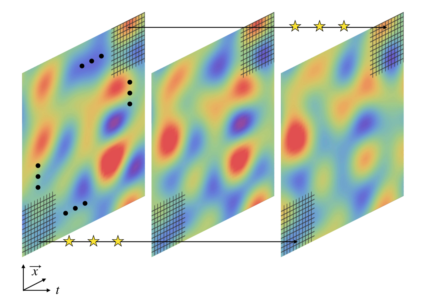
The bubble nucleation algorithm is demonstrated in Fig. 13. We generate the density fluctuations by randomly sampling modes satisfying . We divide the simulation box into small cells (with ), and for each cell we calculate the accumulated nucleation probability in the presence of the density fluctuation as illustrated in Fig. 13. The nucleation time is obtained from random seeds sampled from the range of the accumulated probability. In practice we calculate the time when the expected number of bubbles reaches for each cell, and generate bubbles from up to this point. For each bubble nucleated we assign a random spatial position within each cell. Typically, the first bubble nucleated in each cell will cover the cell quite quickly and the remaining nucleation points are discarded since the first nucleated bubble lies in their past light cone.
Appendix B Analytic expressions
In this section we derive analytic expressions for the bubble nucleation distributions that can be useful when interpreting the results in the main sections.
Without temperature fluctuation
We derive the distribution of the bubble nucleation time. We first neglect the effect of the temperature fluctuation. In this case, the nucleation rate can be written simply as
| (28) |
Here we choose the time so that is satisfied, and label this time as . Though we assume in the following, generalization to is straightforward. For a bubble to nucleate at a given four-dimensional point with an infinitesimal spacetime volume element , we need two conditions (see Fig. 14):
- •
No bubble nucleates inside the past light cone of .
- •
One bubble nucleates in .
The former probability, which we call survival probability , can be expressed as
| (29) |
In the last equality we neglected the effect of cosmic expansion. Together with the latter probability , the nucleation time distribution is
| (30) |
This is plotted as the red lines in Figs. 6 and 6. Note that the overall factor is chosen so that . Note also that the expression before normalizing with gives the average number of bubbles .
With temperature fluctuation
Next we include the temperature fluctuation. While it is difficult to evaluate the final expression analytically, we can extract the IR and UV limits from it. The nucleation rate is
| (31) |
We again take and . The survival probability becomes (see Fig. 14)
| (32) |
and thus the nucleation time distribution averaged over all possible temperature configurations is given by
| (33) |
Here is the ensemble average over the temperature fluctuation. The normalization factor should be chosen so that the total probability becomes unity.

IR and UV limits
We consider the IR limit and the UV limit with fixed . In the IR limit, the temperature is the same over scales much larger than the typical separation between bubbles. Assuming that the temperature fluctuation is Gaussian, and noting that is essentially a time shift, we obtain
| (34) |
We evaluated the expression (34) which yields the red-dotted lines in Figs. 6 and 6.
In the UV limit, the two factors inside the ensemble average of Eq. (33) decouples because an infinite number of temperature fluctuation is realized inside the past cone of . More generally, this argument also allows us to simplify the ensemble-averaged survival probability
| (35) |
The ensemble-averaged nucleation rate just gives a time shift
| (36) |
Therefore, we obtain the following UV limit
| (37) |
References
- [1] LIGO Scientific, Virgo Collaboration, B. Abbott et al., “Observation of Gravitational Waves from a Binary Black Hole Merger,” Phys. Rev. Lett. 116 no. 6, (2016) 061102, arXiv:1602.03837 [gr-qc].
- [2] eLISA Collaboration, P. A. Seoane et al., “The Gravitational Universe,” arXiv:1305.5720 [astro-ph.CO].
- [3] P. Amaro-Seoane, H. Audley, S. Babak, J. Baker, E. Barausse, P. Bender, E. Berti, P. Binetruy, M. Born, D. Bortoluzzi, J. Camp, C. Caprini, V. Cardoso, M. Colpi, J. Conklin, N. Cornish, C. Cutler, K. Danzmann, R. Dolesi, L. Ferraioli, V. Ferroni, E. Fitzsimons, J. Gair, L. G. Bote, D. Giardini, F. Gibert, C. Grimani, H. Halloin, G. Heinzel, T. Hertog, M. Hewitson, K. Holley-Bockelmann, D. Hollington, M. Hueller, H. Inchauspe, P. Jetzer, N. Karnesis, C. Killow, A. Klein, B. Klipstein, N. Korsakova, S. L. Larson, J. Livas, I. Lloro, N. Man, D. Mance, J. Martino, I. Mateos, K. McKenzie, S. T. McWilliams, C. Miller, G. Mueller, G. Nardini, G. Nelemans, M. Nofrarias, A. Petiteau, P. Pivato, E. Plagnol, E. Porter, J. Reiche, D. Robertson, N. Robertson, E. Rossi, G. Russano, B. Schutz, A. Sesana, D. Shoemaker, J. Slutsky, C. F. Sopuerta, T. Sumner, N. Tamanini, I. Thorpe, M. Troebs, M. Vallisneri, A. Vecchio, D. Vetrugno, S. Vitale, M. Volonteri, G. Wanner, H. Ward, P. Wass, W. Weber, J. Ziemer, and P. Zweifel, “Laser interferometer space antenna,” 2017.
- [4] S. R. Coleman, “The Fate of the False Vacuum. 1. Semiclassical Theory,” Phys. Rev. D 15 (1977) 2929–2936. [Erratum: Phys.Rev.D 16, 1248 (1977)].
- [5] A. D. Linde, “Fate of the False Vacuum at Finite Temperature: Theory and Applications,” Phys. Lett. B 100 (1981) 37–40.
- [6] P. J. Steinhardt, “Relativistic Detonation Waves and Bubble Growth in False Vacuum Decay,” Phys. Rev. D 25 (1982) 2074.
- [7] E. Witten, “Cosmic Separation of Phases,” Phys. Rev. D30 (1984) 272–285.
- [8] V. A. Kuzmin, V. A. Rubakov, and M. E. Shaposhnikov, “On the Anomalous Electroweak Baryon Number Nonconservation in the Early Universe,” Phys. Lett. 155B (1985) 36.
- [9] A. G. Cohen, D. Kaplan, and A. Nelson, “Progress in electroweak baryogenesis,” Ann. Rev. Nucl. Part. Sci. 43 (1993) 27–70, arXiv:hep-ph/9302210.
- [10] V. Rubakov and M. Shaposhnikov, “Electroweak baryon number nonconservation in the early universe and in high-energy collisions,” Usp. Fiz. Nauk 166 (1996) 493–537, arXiv:hep-ph/9603208.
- [11] A. Riotto and M. Trodden, “Recent progress in baryogenesis,” Ann. Rev. Nucl. Part. Sci. 49 (1999) 35–75, arXiv:hep-ph/9901362.
- [12] D. E. Morrissey and M. J. Ramsey-Musolf, “Electroweak baryogenesis,” New J. Phys. 14 (2012) 125003, arXiv:1206.2942 [hep-ph].
- [13] C. Caprini et al., “Science with the space-based interferometer eLISA. II: Gravitational waves from cosmological phase transitions,” JCAP 1604 no. 04, (2016) 001, arXiv:1512.06239 [astro-ph.CO].
- [14] R.-G. Cai, Z. Cao, Z.-K. Guo, S.-J. Wang, and T. Yang, “The Gravitational-Wave Physics,” Natl. Sci. Rev. 4 no. 5, (2017) 687–706, arXiv:1703.00187 [gr-qc].
- [15] C. Caprini et al., “Detecting gravitational waves from cosmological phase transitions with LISA: an update,” JCAP 03 (2020) 024, arXiv:1910.13125 [astro-ph.CO].
- [16] E. Barausse et al., “Prospects for Fundamental Physics with LISA,” Gen. Rel. Grav. 52 no. 8, (2020) 81, arXiv:2001.09793 [gr-qc].
- [17] M. B. Hindmarsh, M. Lüben, J. Lumma, and M. Pauly, “Phase transitions in the early universe,” SciPost Phys. Lect. Notes 24 (2021) 1, arXiv:2008.09136 [astro-ph.CO].
- [18] L. Bian et al., “The Gravitational-Wave Physics II: Progress,” arXiv:2106.10235 [gr-qc].
- [19] N. Seto, S. Kawamura, and T. Nakamura, “Possibility of direct measurement of the acceleration of the universe using 0.1-Hz band laser interferometer gravitational wave antenna in space,” Phys. Rev. Lett. 87 (2001) 221103, arXiv:astro-ph/0108011.
- [20] TianQin Collaboration, J. Luo et al., “TianQin: a space-borne gravitational wave detector,” Class. Quant. Grav. 33 no. 3, (2016) 035010, arXiv:1512.02076 [astro-ph.IM].
- [21] W.-R. Hu and Y.-L. Wu, “The Taiji Program in Space for gravitational wave physics and the nature of gravity,” Natl. Sci. Rev. 4 no. 5, (2017) 685–686.
- [22] AEDGE Collaboration, Y. A. El-Neaj et al., “AEDGE: Atomic Experiment for Dark Matter and Gravity Exploration in Space,” EPJ Quant. Technol. 7 (2020) 6, arXiv:1908.00802 [gr-qc].
- [23] A. Sesana et al., “Unveiling the Gravitational Universe at \mu-Hz Frequencies,” arXiv:1908.11391 [astro-ph.IM].
- [24] L. Badurina et al., “AION: An Atom Interferometer Observatory and Network,” JCAP 05 (2020) 011, arXiv:1911.11755 [astro-ph.CO].
- [25] D. Blas and A. C. Jenkins, “Bridging the Hz gap in the gravitational-wave landscape with binary resonance,” arXiv:2107.04601 [astro-ph.CO].
- [26] J. R. Espinosa, T. Konstandin, J. M. No, and G. Servant, “Energy Budget of Cosmological First-order Phase Transitions,” JCAP 1006 (2010) 028, arXiv:1004.4187 [hep-ph].
- [27] F. Giese, T. Konstandin, and J. van de Vis, “Model-independent energy budget of cosmological first-order phase transitions: A sound argument to go beyond the bag model,” JCAP 07 no. 07, (2020) 057, arXiv:2004.06995 [astro-ph.CO].
- [28] F. Giese, T. Konstandin, K. Schmitz, and J. Van De Vis, “Model-independent energy budget for LISA,” JCAP 01 (2021) 072, arXiv:2010.09744 [astro-ph.CO].
- [29] M. Hindmarsh, S. J. Huber, K. Rummukainen, and D. J. Weir, “Gravitational waves from the sound of a first order phase transition,” Phys. Rev. Lett. 112 (2014) 041301, arXiv:1304.2433 [hep-ph].
- [30] M. Hindmarsh, S. J. Huber, K. Rummukainen, and D. J. Weir, “Numerical simulations of acoustically generated gravitational waves at a first order phase transition,” Phys. Rev. D92 no. 12, (2015) 123009, arXiv:1504.03291 [astro-ph.CO].
- [31] M. Hindmarsh, S. J. Huber, K. Rummukainen, and D. J. Weir, “Shape of the acoustic gravitational wave power spectrum from a first order phase transition,” Phys. Rev. D 96 no. 10, (2017) 103520, arXiv:1704.05871 [astro-ph.CO]. [Erratum: Phys.Rev.D 101, 089902 (2020)].
- [32] D. Cutting, M. Hindmarsh, and D. J. Weir, “Vorticity, kinetic energy, and suppressed gravitational wave production in strong first order phase transitions,” Phys. Rev. Lett. 125 no. 2, (2020) 021302, arXiv:1906.00480 [hep-ph].
- [33] R. Jinno, T. Konstandin, and H. Rubira, “A hybrid simulation of gravitational wave production in first-order phase transitions,” JCAP 2104 (2021) 014, arXiv:2010.00971 [astro-ph.CO].
- [34] N. Bartolo, D. Bertacca, S. Matarrese, M. Peloso, A. Ricciardone, A. Riotto, and G. Tasinato, “Anisotropies and non-Gaussianity of the Cosmological Gravitational Wave Background,” Phys. Rev. D 100 no. 12, (2019) 121501, arXiv:1908.00527 [astro-ph.CO].
- [35] V. Domcke, R. Jinno, and H. Rubira, “Deformation of the gravitational wave spectrum by density perturbations,” JCAP 06 (2020) 046, arXiv:2002.11083 [astro-ph.CO].
- [36] T. Bringmann, P. Scott, and Y. Akrami, “Improved constraints on the primordial power spectrum at small scales from ultracompact minihalos,” Phys. Rev. D 85 (2012) 125027, arXiv:1110.2484 [astro-ph.CO].
- [37] M. Sasaki, T. Suyama, T. Tanaka, and S. Yokoyama, “Primordial black holes—perspectives in gravitational wave astronomy,” Class. Quant. Grav. 35 no. 6, (2018) 063001, arXiv:1801.05235 [astro-ph.CO].
- [38] A. Linde, S. Mooij, and E. Pajer, “Gauge field production in supergravity inflation: Local non-Gaussianity and primordial black holes,” Phys. Rev. D 87 no. 10, (2013) 103506, arXiv:1212.1693 [hep-th].
- [39] S. Weinberg, Gravitation and Cosmology. John Wiley and Sons, New York, 1972.
- [40] J. Ellis, M. Lewicki, and J. M. No, “Gravitational waves from first-order cosmological phase transitions: lifetime of the sound wave source,” JCAP 07 (2020) 050, arXiv:2003.07360 [hep-ph].
- [41] M. Maggiore, Gravitational Waves. Vol. 2: Astrophysics and Cosmology. Oxford University Press, 3, 2018.
- [42] G. Jackson and M. Laine, “Hydrodynamic fluctuations from a weakly coupled scalar field,” Eur. Phys. J. C 78 no. 4, (2018) 304, arXiv:1803.01871 [hep-ph].
- [43] K. N. Ananda, C. Clarkson, and D. Wands, “The Cosmological gravitational wave background from primordial density perturbations,” Phys. Rev. D 75 (2007) 123518, arXiv:gr-qc/0612013.
- [44] D. Baumann, P. J. Steinhardt, K. Takahashi, and K. Ichiki, “Gravitational Wave Spectrum Induced by Primordial Scalar Perturbations,” Phys. Rev. D 76 (2007) 084019, arXiv:hep-th/0703290.
- [45] A. Kosowsky, M. S. Turner, and R. Watkins, “Gravitational radiation from colliding vacuum bubbles,” Phys. Rev. D45 (1992) 4514–4535.
- [46] A. Kosowsky and M. S. Turner, “Gravitational radiation from colliding vacuum bubbles: envelope approximation to many bubble collisions,” Phys. Rev. D47 (1993) 4372–4391, arXiv:astro-ph/9211004 [astro-ph].
- [47] S. J. Huber and T. Konstandin, “Gravitational Wave Production by Collisions: More Bubbles,” JCAP 0809 (2008) 022, arXiv:0806.1828 [hep-ph].
- [48] R. Jinno and M. Takimoto, “Gravitational waves from bubble collisions: An analytic derivation,” Phys. Rev. D95 no. 2, (2017) 024009, arXiv:1605.01403 [astro-ph.CO].
- [49] R. Jinno and M. Takimoto, “Gravitational waves from bubble dynamics: Beyond the Envelope,” JCAP 1901 (2019) 060, arXiv:1707.03111 [hep-ph].
- [50] T. Konstandin, “Gravitational radiation from a bulk flow model,” JCAP 1803 no. 03, (2018) 047, arXiv:1712.06869 [astro-ph.CO].
- [51] M. Hindmarsh, “Sound shell model for acoustic gravitational wave production at a first-order phase transition in the early Universe,” Phys. Rev. Lett. 120 no. 7, (2018) 071301, arXiv:1608.04735 [astro-ph.CO].
- [52] M. Hindmarsh and M. Hijazi, “Gravitational waves from first order cosmological phase transitions in the Sound Shell Model,” JCAP 1912 (2019) 062, arXiv:1909.10040 [astro-ph.CO].