跳到论文正文
W Papers独立论文阅读器 arXiv:2108.11828 论文正文 计算阅读时间 · 0%
引用这篇论文根据当前论文元数据生成,正式投稿前建议核对。


License: arXiv.org perpetual non-exclusive license
arXiv:2108.11828v3 [math.NT] 08 Jun 2022

Fourier non-uniqueness sets from totally real number fields

Danylo Radchenko Address: ETH Zürich, Mathematics Department, Rämistrasse 101, 8092 Zürich, Switzerland Email address: danradchenko@gmail.com and Martin Stoller Address: Bâtiment des Mathématiques, EPFL, Station 8, CH-1015 Lausanne, Switzerland Email address: marstoller@gmail.com
Date: August 11, 2026
Abstract.

Let KK be a totally real number field of degree n≥2n\geq 2. The inverse different of KK gives rise to a lattice in ℝn\mathbb{R}^{n}. We prove that the space of Schwartz Fourier eigenfunctions on ℝn\mathbb{R}^{n} which vanish on the “component-wise square root” of this lattice, is infinite dimensional. The Fourier non-uniqueness set thus obtained is a discrete subset of the union of all spheres m​Sn−1\sqrt{m}S^{n-1} for integers m≥0m\geq 0 and, as m→∞m\rightarrow\infty, there are ∼cK​mn−1\sim c_{K}m^{n-1} many points on the mm-th sphere for some explicit constant cKc_{K}, proportional to the square root of the discriminant of KK. This contrasts a recent Fourier uniqueness result by Stoller [17, Cor. 1.1]. Using a different construction involving the codifferent of KK, we prove an analogue for discrete subsets of ellipsoids. In special cases, these sets also lie on spheres with more densely spaced radii, but with fewer points on each.

We also study a related question about existence of Fourier interpolation formulas with nodes “Λ\sqrt{\Lambda}” for general lattices Λ⊂ℝn\Lambda\subset\mathbb{R}^{n}. Using results about lattices in Lie groups of higher rank we prove that if n≥2n\geq 2 and a certain group ΓΛ≤PSL2⁡(ℝ)n\Gamma_{\Lambda}\leq\PSL_{2}(\mathbb{R})^{n} is discrete, then such interpolation formulas cannot exist. Motivated by these more general considerations, we revisit the case of one radial variable and prove, for all n≥5n\geq 5 and all real λ>2\lambda>2, Fourier interpolation results for sequences of spheres 2​m/λ​Sn−1\sqrt{2m/\lambda}S^{n-1}, where mm ranges over any fixed cofinite set of non-negative integers. The proof relies on a series of Poincaré type for Hecke groups of infinite covolume and is similar to the one in [17, §4].

1. Introduction

The subject of this paper is motivated by recent work on Fourier uniqueness and non-uniqueness pairs. Broadly speaking, we are interested in the following general question. Given a space VV of continuous integrable functions on ℝn\mathbb{R}^{n} and two subsets A,B⊂ℝnA,B\subset\mathbb{R}^{n}, when is it possible to recover any function f∈Vf\in V from the restrictions f|Af|_{A} and f^|B\widehat{f}|_{B} (where f^\widehat{f} denotes the Fourier transform of ff)? In other words, we are interested in conditions on A,B,VA,B,V, under which the restriction map f↦(f|A,f^|B)f\mapsto(f|_{A},\widehat{f}|_{B}) is injective. When the map is injective, we say that (A,B)(A,B) is a (Fourier) uniqueness pair and if A=BA=B, we simply say that AA is a (Fourier) uniqueness set. Conversely, if the map is not injective, we call (A,B)(A,B) a non-uniqueness pair, and when A=BA=B we call AA a non-uniqueness set. Naturally, one would like the function space VV to be as large as possible and the sets AA and BB to be as small as possible, or “minimal” in a certain sense.

A prototypical example of a minimal Fourier uniqueness set was found by Radchenko and Viazovska in [12], where they proved that, when V=𝒮even​(ℝ)V=\mathcal{S}_{\text{even}}(\mathbb{R}) is the space of even Schwartz functions on the real line, the set A=ℤ+:={n:n∈ℤ≥0}A=\sqrt{\mathbb{Z}_{+}}:=\{\sqrt{n}\,:\,n\in\mathbb{Z}_{\geq 0}\} is a uniqueness set and established an interpolation theorem in this setting. The result is sharp in the sense that no proper subset of AA remains a uniqueness set for 𝒮even​(ℝ)\mathcal{S}_{\text{even}}(\mathbb{R}). Their proof was based on the theory of classical modular forms, which is also well-suited to treat the case V=𝒮rad​(ℝn)V=\mathcal{S}_{\text{rad}}(\mathbb{R}^{n}) of radial Schwartz functions on ℝn\mathbb{R}^{n} and the set A=Un:=∪m∈ℕ0mSn−1A=U_{n}:=\cup_{m\in\mathbb{N}_{0}}{\sqrt{m}S^{n-1}}. For the latter generalization, we refer to §2 in [13], which deduces the result from [4].

The second author recently proved an interpolation formula [17, Thm 1] generalizing the one by Radchenko–Viazovska also to non-radial functions, that is, to the space V=𝒮⁡(ℝn)V=\mathcal{S}(\mathbb{R}^{n}) and the same set of concentric spheres UnU_{n}. However, for n>1n>1, it is no longer minimal. Indeed, the (related) interpolation formula in [13, Eq. (4.1)] implies that the space of f∈𝒮⁡(ℝn)f\in\mathcal{S}(\mathbb{R}^{n}) satisfying f​(x)=f^​(x)=0f(x)=\widehat{f}(x)=0 for all x∈∪m≥NmSn−1x\in\cup_{m\geq N}{\sqrt{m}S^{n-1}} is finite-dimensional for all NN and is in fact contained in ℋ4​N+2⊗W\mathcal{H}_{4N+2}\otimes W for some finite-dimensional space W⊂𝒮rad​(ℝn)W\subset\mathcal{S}_{\text{rad}}(\mathbb{R}^{n}), where ℋk\mathcal{H}_{k} denotes the space of harmonic polynomials on ℝn\mathbb{R}^{n} of degree ≤k\leq k. Since a generic subset of dimℋk\dim\mathcal{H}_{k} points in r​Sn−1rS^{n-1} is an interpolation set for the space ℋk\mathcal{H}_{k} (in the sense that any polynomial p∈ℋkp\in\mathcal{H}_{k} is uniquely determined by its values on dimℋk\dim\mathcal{H}_{k} generic points), this implies that there is a uniqueness set properly contained in UnU_{n} that contains only finitely many points on spheres with radius ≤N\leq\sqrt{N}.

In fact, it was recently proved by the second author and Ramos in [13, Rmk 4.1, Cor 4.1] that any discrete and sufficiently uniformly distributed subset D⊂UnD\subset U_{n} remains a uniqueness set for 𝒮⁡(ℝn)\mathcal{S}(\mathbb{R}^{n}). Here, “sufficiently” means that D∩m​Sn−1D\cap\sqrt{m}S^{n-1} contains at least Cn​mcn​mC_{n}m^{c_{n}m} many points.

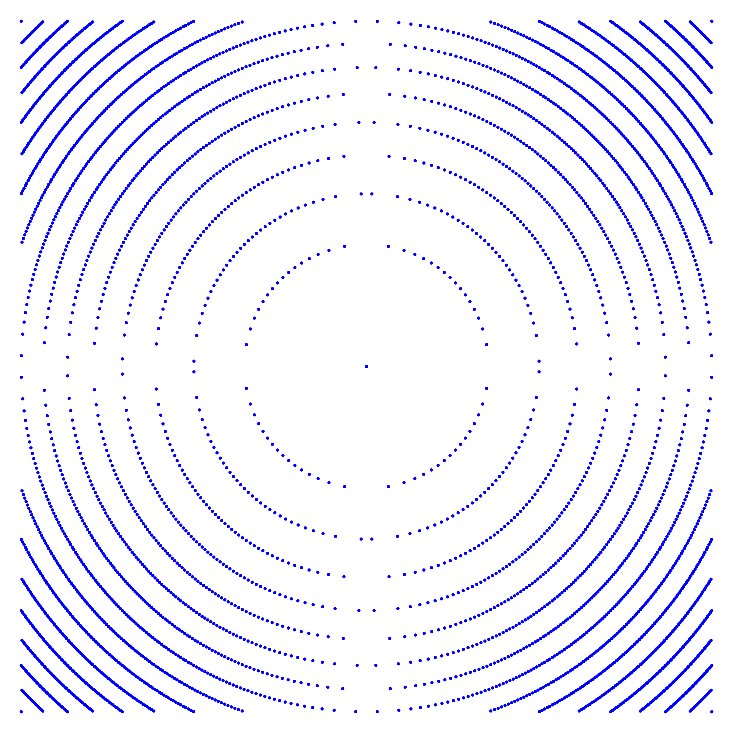
We contrast these Fourier uniqueness results by providing two families of discrete non-uniqueness sets in ℝn\mathbb{R}^{n}, where one of them is again contained UnU_{n}, while the other lies in a union of ellipsoids. Both of them are constructed from lattices corresponding to ideals in totally real number fields K/ℚK/\mathbb{Q} of degree nn and their density grows with the discriminant of KK (although their distribution is not uniform, in the sense that they “avoid” points near the coordinate axes; see Figure 1). We give the precise formulations in the next subsection. Thus, characterizing the discrete Fourier uniqueness sets contained in UnU_{n} seems to be a subtle question.

In fact, the motivation for this work was not to find negative results in this direction, but to try to generalize the modular form theoretic approach of Radchenko and Viazovska to treat not necessarily radial functions on ℝn\mathbb{R}^{n}, in a way that is very different from the approach taken by Stoller (who essentially reduces the problem again to the case of radial Schwartz functions). More specifically, we were interested in (possible) interpolation formulas where we replace the set of nodes A=ℤ+A=\sqrt{\mathbb{Z}_{+}} by “square roots” of certain lattices coming from totally real number fields KK, specifically, the co-different 𝒪K∨\mathcal{O}_{K}^{\vee} of their ring of integers 𝒪K\mathcal{O}_{K}. In this set up, it seemed natural to ask whether one could be working with Hilbert modular forms and associated integral transforms, similarly to the proof by Radchenko–Viazovska.

As we will explain more in §4 and briefly in §1.6, there is an obstruction to the existence of such interpolation formulas. From the more general point of view taken in §4, the obstruction arises because, for n≥2n\geq 2, subgroups of PSL2⁡(ℝ)n\PSL_{2}(\mathbb{R})^{n} that are commensurable to the Hilbert modular group PSL2⁡(𝒪K)\PSL_{2}(\mathcal{O}_{K}) are irreducible lattices and can therefore never contain subgroups of finite index with infinite abelianization, by Margulis’ normal subgroup theorem. On the other hand the presence of certain unfavorable relations in the Hilbert modular group can be exploited in an explicit manner to obtain the non-uniqueness sets indicated in the abstract.

1.1. Statement of non-uniqueness results

We prepare for the formulation of our main non-uniqueness results and at the same time, introduce some notation that will be used throughout the paper. Let KK be a totally real number field of degree n≥2n\geq 2 with ring of integers 𝒪K\mathcal{O}_{K}. Some of the objects we will introduce depend on the number field KK, but we will not always display this dependence in our notation.

We denote the nn real embeddings by σj:K→ℝ\sigma_{j}:K\rightarrow\mathbb{R}, 1≤j≤n1\leq j\leq n and assemble them into the map σ:K→ℝn\sigma:K\rightarrow\mathbb{R}^{n}, σ⁡(x)=(σ1​(x),…,σn​(x))\sigma(x)=(\sigma_{1}(x),\dots,\sigma_{n}(x)). We recall that the trace of an element x∈Kx\in K is given by Tr⁡(x)=TrK/ℚ⁡(x)=∑j=1nσj​(x)\Tr(x)=\Tr_{K/\mathbb{Q}}(x)=\sum_{j=1}^{n}{\sigma_{j}(x)}. For any 𝒪K\mathcal{O}_{K}-submodule 𝔞⊂K\mathfrak{a}\subset K we write

𝔞∨={x∈K:TrK/ℚ(ax)∈ℤfor all a∈𝔞}\mathfrak{a}^{\vee}=\left\{x\in K\,:\,\,\Tr_{K/\mathbb{Q}}(ax)\in\mathbb{Z}\,\;\mbox{for all }a\in\mathfrak{a}\right\}

for its dual with respect to the trace paring. As is well-known, if 𝔞\mathfrak{a} is a fractional ideal in KK, then σ⁡(𝔞)⊂ℝn\sigma(\mathfrak{a})\subset\mathbb{R}^{n} is a lattice and σ⁡(𝔞∨)=σ​(𝔞)∨\sigma(\mathfrak{a}^{\vee})=\sigma(\mathfrak{a})^{\vee}, where on the right we mean the dual lattice in the usual sense. Moreover, the covolume of σ⁡(𝔞)\sigma(\mathfrak{a}) is given by

(1.1) covol⁡(σ⁡(𝔞))=N⁡(𝔞)​|disc⁡(K)|,\covol{(\sigma(\mathfrak{a}))}=\Nr(\mathfrak{a})\sqrt{|\disc(K)|},

where N⁡(𝔞)∈ℚ>0\Nr(\mathfrak{a})\in\mathbb{Q}_{>0} is the ideal norm of 𝔞\mathfrak{a} (the unique extension of the absolute norm on integral ideals to all fractional ideals of KK) and |disc⁡(K)|=covol⁡(σ⁡(𝒪K))2|\disc(K)|=\covol(\sigma(\mathcal{O}_{K}))^{2} is the discriminant of KK. For any fractional ideal 𝔞⊂K\mathfrak{a}\subset K we define

(1.2) 𝔞:=σ⁡(𝔞):={(x1,…,xn)∈ℝn:(x12,…,xn2)=σ⁡(α)​ for some ​α∈𝔞}⊂ℝn\sqrt{\mathfrak{a}}:=\sqrt{\sigma(\mathfrak{a})}:=\left\{(x_{1},\dots,x_{n})\in\mathbb{R}^{n}\,:\,(x_{1}^{2},\dots,x_{n}^{2})=\sigma(\alpha)\,\text{ for some }\alpha\in\mathfrak{a}\right\}\subset\mathbb{R}^{n}

(which is not to be confused with the radical of an ideal). Recall that the codifferent (or inverse different) of KK is the fractional ideal 𝒪K∨\mathcal{O}_{K}^{\vee} and that the different 𝔡=𝔡K\mathfrak{d}=\mathfrak{d}_{K} is defined as 𝔡=(𝒪K∨)−1\mathfrak{d}=(\mathcal{O}_{K}^{\vee})^{-1}. We see that the points 𝒪K∨\sqrt{\mathcal{O}_{K}^{\vee}} lie on spheres m​Sn−1\sqrt{m}S^{n-1} with non-negative integers mm, the traces of the totally non-negative elements in 𝒪K∨\mathcal{O}_{K}^{\vee} (recall that an element x∈Kx\in K is said to be totally non-negative (resp. totally positive) if σj​(x)≥0\sigma_{j}(x)\geq 0 (resp. σj​(x)>0\sigma_{j}(x)>0) for all j=1,…,nj=1,\dots,n). We return to these points in §1.2.

For f∈L1​(ℝn)f\in L^{1}(\mathbb{R}^{n}) we normalize its Fourier transform by f^​(ξ)=∫ℝnf⁡(x)​e−2​π​i​⟨x,ξ⟩​𝑑x\widehat{f}(\xi)=\int_{\mathbb{R}^{n}}{f(x)e^{-2\pi i\langle x,\xi\rangle}dx}, ξ∈ℝn\xi\in\mathbb{R}^{n}. We sometimes also use the notation ℱ⁡(f)=ℱℝn​(f)=f^\mathcal{F}(f)=\mathcal{F}_{\mathbb{R}^{n}}(f)=\widehat{f}. Finally, we write ℍ={z∈ℂ:Im⁡(z)>0}\mathbb{H}=\{z\in\mathbb{C}\,:\,\imag(z)>0\} for the upper half plane.

Theorem 1.

Let KK be a totally real number field of degree n≥2n\geq 2 as above. Let V⊂𝒮⁡(ℝn)V\subset\mathcal{S}(\mathbb{R}^{n}) denote the subspace linearly spanned by all Gaussians eπ​i​z1​x12⋯eπ​i​zn​xn2e^{\pi iz_{1}x_{1}^{2}}\cdots e^{\pi iz_{n}x_{n}^{2}} with zj∈ℍz_{j}\in\mathbb{H}, xj∈ℝx_{j}\in\mathbb{R}. Then for any ϵ∈{±1}\epsilon\in\{\pm 1\} the subspace of all f∈Vf\in V satisfying f⁡(x)=0f(x)=0 for all x∈𝒪K∨x\in\sqrt{\mathcal{O}_{K}^{\vee}} and f^=ϵ​f\widehat{f}=\epsilon f is infinite dimensional.

Remark 1.1.

Since the space of Fourier eigenfunctions vanishing on 𝒪K∨\sqrt{\mathcal{O}_{K}^{\vee}} is infinite-dimensional we can obtain nontrivial functions vanishing in addition on an arbitrary finite subset of ℝn\mathbb{R}^{n}, by a simple linear algebra argument. A similar remark applies to Theorem 2 below.

Besides points on spheres m​Sn−1\sqrt{m}S^{n-1}, our methods also allow us to treat other sets related to the different, which in general lie on ellipsoids. To formulate it, we appeal to a Theorem of Hecke [7, §63, Satz 176], asserting that the different 𝔡\mathfrak{d} defines a square in the ideal class group of KK. This means that we can choose a fractional ideal 𝔞\mathfrak{a} and a scalar c∈K×c\in K^{\times} such that

(1.3) c​𝔞2=𝔡−1.c\mathfrak{a}^{2}=\mathfrak{d}^{-1}.

Let us then define the set

(1.4) E⁡(c,𝔞):={x∈ℝn:∃α∈𝔞2​ such that ​σ​(α)=(x12/|σ1​(c)|,…,xn2/|σn​(c)|)}.E(c,\mathfrak{a}):=\left\{x\in\mathbb{R}^{n}\,:\,\exists\alpha\in\mathfrak{a}^{2}\text{ such that }\sigma(\alpha)=(x_{1}^{2}/|\sigma_{1}(c)|,\dots,x_{n}^{2}/|\sigma_{n}(c)|)\right\}.

Note that this is a discrete subset of a union of ellipsoids in ℝn\mathbb{R}^{n}.

Theorem 2.

Let KK, nn, and VV be as in Theorem 1 and let cc and 𝔞\mathfrak{a} be such that (1.3) holds. Then, for every ϵ∈{±1}\epsilon\in\{\pm 1\} the subspace of all f∈Vf\in V satisfying f⁡(x)=0f(x)=0 for all x∈E⁡(c,𝔞)x\in E(c,\mathfrak{a}) and f^=ϵ​f\widehat{f}=\epsilon f is infinite dimensional.

The functions we produce for Theorems 1 and 2 are quite explicit. The prototypical example is a linear combination of 16 Gaussians whose parameters z∈ℍnz\in\mathbb{H}^{n} are of the form z=γ⋅τz=\gamma\cdot\tau for a generic point τ∈ℍn\tau\in\mathbb{H}^{n} and some special elements γ∈PSL2⁡(𝒪K)\gamma\in\PSL_{2}(\mathcal{O}_{K}), eight of which are written down explicitly in the proof of Proposition 2.1. The entries of the matrices can be computed if one knows some non-trivial units of 𝒪K\mathcal{O}_{K} in the congruence classes 1+4​𝒪K1+4\mathcal{O}_{K} and 1+3​𝒪K1+3\mathcal{O}_{K}.

In the remaining parts of this introduction we give further explanations for Theorems 1 and 2 and add a few remarks. In §1.6, we describe the other two results indicated in the abstract.

1.2. On the number of points in 𝔡−1∩m​Sn−1\sqrt{\mathfrak{d}^{-1}}\cap\sqrt{m}S^{n-1}

The cardinality of 𝔡−1∩m​Sn−1\sqrt{\mathfrak{d}^{-1}}\cap\sqrt{m}S^{n-1} is 2n2^{n} times the number of totally non-negative elements in 𝔡−1\mathfrak{d}^{-1} of trace m≥0m\geq 0. By choosing a ℤ\mathbb{Z}-basis for 𝒪K\mathcal{O}_{K} containing 11 and considering the element α1∈K\alpha_{1}\in K such that the ℚ\mathbb{Q}-linear functional y↦Tr⁡(α1​y)y\mapsto\Tr(\alpha_{1}y) takes the value 11 on y=1y=1 and zero on all other elements of the basis, we see that Tr⁡(α1)=1\Tr(\alpha_{1})=1 and α1∈𝔡−1\alpha_{1}\in\mathfrak{d}^{-1}. It follows that for all m∈ℤm\in\mathbb{Z}, we have

{α∈𝔡−1:Tr⁡(α)=m}=m​α1+(𝔡−1)0,(𝔡−1)0:={α∈𝔡−1:Tr⁡(α)=0}.\{\alpha\in\mathfrak{d}^{-1}\,:\,\Tr(\alpha)=m\}=m\alpha_{1}+(\mathfrak{d}^{-1})_{0},\qquad(\mathfrak{d}^{-1})_{0}:=\{\alpha\in\mathfrak{d}^{-1}\,:\,\Tr(\alpha)=0\}.

Thus, for m≥0m\geq 0, the subset of ℝn\mathbb{R}^{n} whose cardinality we are interested in, can be written as

(mσ(α1)+σ((𝔡−1)0))∩[0,∞)n\left(m\sigma(\alpha_{1})+\sigma((\mathfrak{d}^{-1})_{0})\right)\cap[0,\infty)^{n}

whose cardinality equals that of

σ((𝔡−1)0)∩m([0,∞)n−σ(α1))\sigma((\mathfrak{d}^{-1})_{0})\cap m([0,\infty)^{n}-\sigma(\alpha_{1}))

which is the set of lattice points of σ⁡((𝔡−1)0)⊂{x∈ℝn:∑i=1nxi=0}\sigma((\mathfrak{d}^{-1})_{0})\subset\{x\in\mathbb{R}^{n}\,:\,\sum_{i=1}^{n}{x_{i}}=0\} in a homogeneously expanding (n−1)(n-1)-dimensional region, allowing for an application of a standard estimate of the number of such points, as m→∞m\rightarrow\infty. The necessary volume computations are done (for any fractional ideal, in fact) in the work of Ash and Friedberg, see [1, §5, Prop. 5.1 and §6]. From the cited parts of their work, we deduce that

(1.5) |𝔡−1∩m​Sn−1|=2n​|disc⁡(K)|(n−1)!​mn−1+O⁡(mn−2),m→∞,\left|\sqrt{\mathfrak{d}^{-1}}\cap\sqrt{m}S^{n-1}\right|=2^{n}\frac{\sqrt{|\disc(K)|}}{(n-1)!}m^{n-1}+O(m^{n-2}),\quad m\rightarrow\infty,

where the implied constant may depend on KK and nn. We point out the following features of this asymptotic formula:

  • •

    The surface area of m​Sn−1\sqrt{m}S^{n-1} grows like mn−12m^{\frac{n-1}{2}}, so the points are more densely spaced than a constant number of points per unit surface area on Sn−1S^{n-1}.

  • •

    We may increase the density of points by a constant factor, by taking the discriminant of KK arbitrarily large, while keeping the degree nn fixed.

  • •

    For small mm, there may be no points in 𝔡−1∩m​Sn−1\sqrt{\mathfrak{d}^{-1}}\cap\sqrt{m}S^{n-1}, but note that we can add any finite set of points on these small spheres, by Remark 1.1.
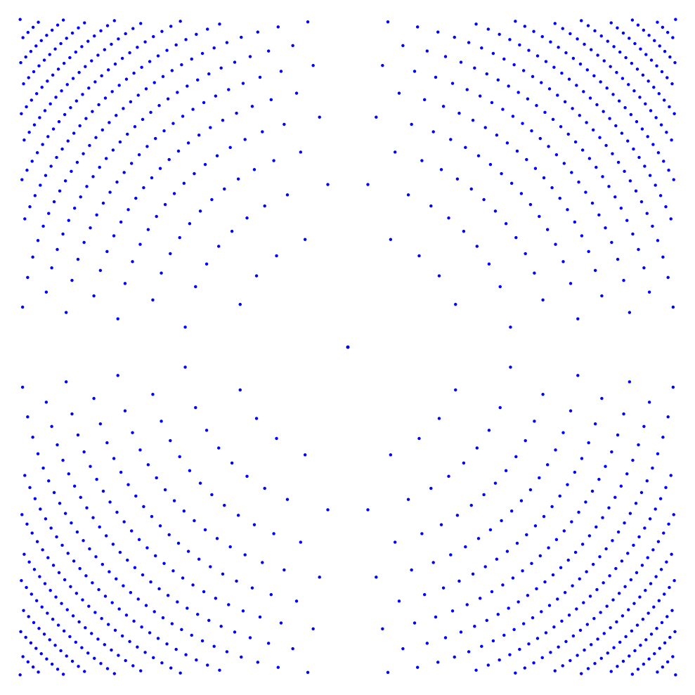
Refer to caption
Refer to caption
Figure 1. Non-uniqueness sets constructed from ℚ⁡(17)\mathbb{Q}(\sqrt{17}) and ℚ⁡(257)\mathbb{Q}(\sqrt{257})

1.3. The relation between Theorem 1 and Theorem 2

If the number cc in (1.3) can be taken totally positive, then E⁡(c,𝔞)=𝒪K∨E(c,\mathfrak{a})=\sqrt{\mathcal{O}_{K}^{\vee}} and both theorems give the same result. Since we are free to replace cc by ε​c\varepsilon c for any unit ε∈𝒪K×\varepsilon\in\mathcal{O}_{K}^{\times}, we can take cc totally positive, provided KK has units ε\varepsilon of all possible sign patterns (σj​(ε)/|σj​(ε)|)1≤j≤n∈{±1}n(\sigma_{j}(\varepsilon)/|\sigma_{j}(\varepsilon)|)_{1\leq j\leq n}\in\{\pm 1\}^{n}. In the real quadratic case, the latter is equivalent to the fundamental unit having norm −1-1. Such conditions are studied more generally in the literature, via the notion of signature rank.

In fact, whenever K/ℚK/\mathbb{Q} is Galois and nn is odd, then c=1c=1 is admissible. In other words, the different is then exactly equal to the square of another ideal. This follows from Hilbert’s formula, see [10, Ex. 5.45, p. 253].

Generally, recall that a large class of number fields which allows for an easy determination of admissible cc and 𝔞\mathfrak{a} in (1.3) is given by monogenic number fields. For example, for any irreducible monic polynoimal P∈ℤ⁡[X]P\in\mathbb{Z}[X] with square-free discriminant and no complex roots, we can take K=ℚ⁡(α)⊂ℝK=\mathbb{Q}(\alpha)\subset\mathbb{R} for some root α\alpha of PP. Then it is well-known that 𝒪K=ℤ⁡[α]\mathcal{O}_{K}=\mathbb{Z}[\alpha] and 𝒪K∨=1P′​(α)​𝒪K\mathcal{O}_{K}^{\vee}=\frac{1}{P^{\prime}(\alpha)}\mathcal{O}_{K}, so that (c,𝔞)=(1/P′​(α),𝒪K)(c,\mathfrak{a})=(1/P^{\prime}(\alpha),\mathcal{O}_{K}) is admissible in (1.3).

We note further that, if there is a constant θ>0\theta>0 so that |σj​(c)|=θ|\sigma_{j}(c)|=\theta for all j=1,…,nj=1,\dots,n, then the set E⁡(c,𝔞)E(c,\mathfrak{a}) is contained in the union of spheres θ​m​Sn−1\sqrt{\theta m}S^{n-1} (rather than in a union ellipsoids). This happens for some real-quadratic fields, see §1.4.

1.4. Real quadratic fields

To illustrate the theorems in the case n=2n=2, consider a real quadratic field K=ℚ⁡(D)K=\mathbb{Q}(\sqrt{D}) as a subfield of ℝ\mathbb{R} of discriminant D,D>0D,\sqrt{D}>0 and for x∈Kx\in K write σ1​(x)=x\sigma_{1}(x)=x and σ2​(x)=:x′\sigma_{2}(x)=:x^{\prime} so that D′=−D\sqrt{D}^{\prime}=-\sqrt{D}. Define ω:=(D+D)/2\omega:=(D+\sqrt{D})/2 and c:=1/Dc:=1/\sqrt{D}. Then 𝒪K=ℤ+ℤ​ω\mathcal{O}_{K}=\mathbb{Z}+\mathbb{Z}\omega and 𝒪K∨=c​𝒪K=c​𝒪K2\mathcal{O}_{K}^{\vee}=c\mathcal{O}_{K}=c\mathcal{O}_{K}^{2} (square of a fractional ideal). Thus, every element of 𝒪K∨\mathcal{O}_{K}^{\vee} may be written as α=c⁡(ℓ+m​ω)\alpha=c(\ell+m\omega) for ℓ,m∈ℤ\ell,m\in\mathbb{Z} and has Tr⁡(α)=ℓ​Tr⁡(c)+m​Tr⁡(ω​c)=m\Tr(\alpha)=\ell\Tr(c)+m\Tr(\omega c)=m. The element α\alpha is totally non-negative if and only if m≥0m\geq 0 and −m​ω≤ℓ≤−m​ω′-m\omega\leq\ell\leq-m\omega^{\prime}. This shows that

|𝒪K∨∩m​S1|=2​|ℤ∩[−m​ω,−m​ω′]|∼2​m​D,m→∞,\left|\sqrt{\mathcal{O}_{K}^{\vee}}\cap\sqrt{m}S^{1}\right|=2\left|\mathbb{Z}\cap[-m\omega,-m\omega^{\prime}]\right|\sim 2m\sqrt{D},\quad m\rightarrow\infty,

which exemplifies (1.5) and Theorem 1 in the simplest case.

Let us now illustrate Theorem 2 with 𝔞=𝒪K\mathfrak{a}=\mathcal{O}_{K} and the above value of cc, which is not totally positive and satisfies |σ1​(c)|=|σ2​(c)|=1D|\sigma_{1}(c)|=|\sigma_{2}(c)|=\frac{1}{\sqrt{D}}. We assume that 4|D4|D and set d:=D/4≡2,3(mod4)d:=D/4\equiv 2,3\pmod{4}, so that 𝒪K=ℤ+ℤ​d\mathcal{O}_{K}=\mathbb{Z}+\mathbb{Z}\sqrt{d}. Then E⁡(c,𝔞)E(c,\mathfrak{a}) is the set of x=(x1,x2)∈ℝ2x=(x_{1},x_{2})\in\mathbb{R}^{2} such that

(x12,x22)=12​d​(a+b​d,a−b​d)(x_{1}^{2},x_{2}^{2})=\frac{1}{2\sqrt{d}}\left(a+b\sqrt{d},a-b\sqrt{d}\right)

for some a,b∈ℤa,b\in\mathbb{Z} satisfying |b​d|≤a|b\sqrt{d}|\leq a and x12+x22=adx_{1}^{2}+x_{2}^{2}=\frac{a}{\sqrt{d}}. In other words, E⁡(c,𝔞)E(c,\mathfrak{a}) is a discrete subset of a union of circles of radii a/d\sqrt{a/\sqrt{d}}, for all integers a≥0a\geq 0 with about a/da/\sqrt{d} many points on each. If D≡1(mod4)D\equiv 1\pmod{4}, then E⁡(c,𝔞)E(c,\mathfrak{a}) is a discrete subset of the union of all circles of radii t/D\sqrt{t/\sqrt{D}} for all integers t≥0t\geq 0 with about 2​t/D2t/\sqrt{D} points on each.

1.5. A minor generalization of Theorem 1

The space of Gaussians defined in Theorem 1 is a subspace of the space of Schwartz functions on ℝn\mathbb{R}^{n} that are even in each variable (and it turns out to be dense in that space, see Proposition 4.1). More generally, Theorem 1 holds and will be proved in the following setting.

Let d,n≥1d,n\geq 1 be integers and consider a partition d=d1+⋯+dnd=d_{1}+\dots+d_{n} of dd. We view the Euclidean space ℝd\mathbb{R}^{d} as the product space ℝd1×⋯×ℝdn\mathbb{R}^{d_{1}}\times\dots\times\mathbb{R}^{d_{n}} and elements x∈ℝdx\in\mathbb{R}^{d} as nn-tuples x=(x1,…,xn)x=(x_{1},\dots,x_{n}) where xj∈ℝdjx_{j}\in\mathbb{R}^{d_{j}}. The group O⁡(d1)×⋯×O⁡(dn)\Or(d_{1})\times\dots\times\Or(d_{n}) embeds block-diagonally into the orthogonal group O⁡(d)\Or(d). Denote by 𝒮​(ℝd)O⁡(d1)×⋯×O⁡(dn)\mathcal{S}(\mathbb{R}^{d})^{\Or(d_{1})\times\dots\times\Or(d_{n})} the space of Schwartz functions on ℝd\mathbb{R}^{d} that are radial in each of the nn variables xj∈ℝdjx_{j}\in\mathbb{R}^{d_{j}}. Such functions can be identified with functions on [0,+∞)n[0,+\infty)^{n} and we freely use this identification to evaluate them on nn-tuples of non-negative real numbers. An O⁡(d1)×⋯×O⁡(dn)\Or(d_{1})\times\dots\times\Or(d_{n})-invariant function on ℝd\mathbb{R}^{d} will be said to vanish on 𝒪K∨\sqrt{\mathcal{O}_{K}^{\vee}}, if f⁡(x)=0f(x)=0 for all x∈ℝdx\in\mathbb{R}^{d} such that (|x1|2,…,|xn|2)=(σ1​(α),…,σn​(α))(|x_{1}|^{2},\dots,|x_{n}|^{2})=(\sigma_{1}(\alpha),\dots,\sigma_{n}(\alpha)) for some α∈𝒪K∨\alpha\in\mathcal{O}_{K}^{\vee}.

Besides the case where all djd_{j} are equal, our proof of Theorem 2 does not seem to easily generalize to the more general setting that we have just described, for technical reasons having to do with the existence of automorphic factors, see §2.

1.6. General lattices and a radial uniqueness result

As already mentioned above, in §4 we will consider general lattices Λ⊂ℝn\Lambda\subset\mathbb{R}^{n} and their square roots Λ:={(x1,…,xn)∈ℝn:(x12,…,xn2)∈Λ}\sqrt{\Lambda}:=\{(x_{1},\dots,x_{n})\in\mathbb{R}^{n}\,:\,(x_{1}^{2},\dots,x_{n}^{2})\in\Lambda\}. In §4.1, we will explain (mainly for motivational purposes) a natural equivalent formulation of a Fourier interpolation formula using the pair of sets (Λ1,Λ2)(\sqrt{\Lambda_{1}},\sqrt{\Lambda_{2}}) for lattices Λ1,Λ2⊂ℝn\Lambda_{1},\Lambda_{2}\subset\mathbb{R}^{n} in terms of generating series, viewed as functions on ℍn\mathbb{H}^{n} and describe their modular transformation properties in terms of a certain subgroup Γ⁡(L1,L2)≤PSL2⁡(ℝ)n\Gamma(L_{1},L_{2})\leq\PSL_{2}(\mathbb{R})^{n}, where Li=2​Λi∨L_{i}=2\Lambda_{i}^{\vee}. We will prove in Proposition 4.3 that, for n≥2n\geq 2, there is no pair of lattices (L1,L2)(L_{1},L_{2}) such that the group Γ⁡(L1,L2)\Gamma(L_{1},L_{2}) is discrete and at the same time the free inner product of two subgroups of upper- and lower triangular elements isomorphic to L1L_{1} and L2L_{2} respectively. We prove that the latter property of Γ⁡(L1,L2)\Gamma(L_{1},L_{2}) is a necessary condition for the existence of such an interpolation formula (Proposition 4.2) and we argue why discreteness might be necessary as well.

From this more general point of view we return in §5 to the case n=1n=1 and prove:

Theorem (== Theorem 3 ++ Corollary 5.1 in §5).

For all d≥5d\geq 5 and all positive reals α,β\alpha,\beta such that α​β≥1\alpha\beta\geq 1 the pair

(1.6) (∪m≥1m/αSd−1,∪m≥1m/βSd−1)\left(\cup_{m\geq 1}{\sqrt{m/\alpha}S^{d-1}},\cup_{m\geq 1}{\sqrt{m/\beta}S^{d-1}}\right)

is a Fourier uniqueness pair for 𝒮⁡(ℝd)\mathcal{S}(\mathbb{R}^{d}) and there exists a linear interpolation formula which proves this. Furthermore, if α​β>1\alpha\beta>1, then (1.6) remains a uniqueness pair after removing any finite number of spheres from both sides.

The radial interpolation result (Theorem 3) will be proved via a series construction generalizing the one used in [17] from Γ⁡(2)\Gamma(2) to the subgroup of PSL2⁡(ℝ)\PSL_{2}(\mathbb{R}) generated by

(12​α01),(102​β1).\begin{pmatrix}1&2\alpha\\ 0&1\end{pmatrix},\qquad\begin{pmatrix}1&0\\ 2\beta&1\end{pmatrix}.

For α​β≥1\alpha\beta\geq 1, it is conjugate in PSL2⁡(ℝ)\PSL_{2}(\mathbb{R}) to a normal subgroup of index two in a Hecke group and is isomorphic to Γ⁡(2)\Gamma(2). For α​β>1\alpha\beta>1 these groups have infinite covolume and infinite dimensional spaces of modular forms. The latter fact was proved by Hecke [6, §3] and his construction of linearly independent modular forms allows us to remove finitely many spheres from (1.6).

1.7. Some notation

Besides the notation introduced above, we will also use the following general notation throughout the paper. For z∈ℍz\in\mathbb{H}, the number z/iz/i belongs to the right half plane ℋ:={w∈ℂ:Re⁡(w)>0}\mathcal{H}:=\{w\in\mathbb{C}\,:\,\real(w)>0\} and on it, we always use the branch of the logarithm w↦log⁡(w)w\mapsto\log(w) that takes real values on (0,+∞)(0,+\infty). For any z∈ℍz\in\mathbb{H} and k∈ℂk\in\mathbb{C}, we thus define (z/i)k=exp⁡(k​log⁡(z/i))(z/i)^{k}=\exp(k\log(z/i)). For x∈ℝx\in\mathbb{R} we define sgn⁡(x)∈{−1,0,1}\sgn(x)\in\{-1,0,1\} as sgn⁡(x)=x/|x|\sgn(x)=x/|x| if x≠0x\neq 0 and sgn⁡(0):=0\sgn(0):=0.

In the setting of §1.5 we will work with complex Gaussians, parameterized by points z=(z1,…,zn)∈ℍnz=(z_{1},\dots,z_{n})\in\mathbb{H}^{n} and defined as

(1.7) g(z,x)=eπ​i​z1​|x1|2⋯eπ​i​zn​|xn|2,xj∈ℝdj.g(z,x)=e^{\pi iz_{1}|x_{1}|^{2}}\cdots e^{\pi iz_{n}|x_{n}|^{2}},\quad x_{j}\in\mathbb{R}^{d_{j}}.

We sometimes also view gg as a map g:ℍn→𝒮(ℝd)O(d1)×⋯×O(dn)g:\mathbb{H}^{n}\rightarrow\mathcal{S}(\mathbb{R}^{d})^{\Or(d_{1})\times\cdots\times\Or(d_{n})}, so that from this point of view g​(z)​(x)=g​(z,x)g(z)(x)=g(z,x). Moreover, we have, for all z∈ℍnz\in\mathbb{H}^{n},

(1.8) g⁡(z)^=(z1/i)−d1/2⋯(zn/i)−dn/2g(−1/z),−1/z:=(−1/z1,…,−1/zn).\widehat{g(z)}=(z_{1}/i)^{-d_{1}/2}\cdots(z_{n}/i)^{-d_{n}/2}g(-1/z),\quad-1/z:=(-1/z_{1},\dots,-1/z_{n}).

More specific notation will be introduced in the body of the paper.

Acknowledgments

The second author would like to thank Maryna Viazovska for sharing ideas and techniques during his previous work [17], which were also useful in §5.

2. Proof of Theorem 2

The goal of this section is to prove Theorem 2. In §2.1 we introduce some notation and define a “theta-subgroup” Γϑ\Gamma_{\vartheta} of the Hilbert modular group PSL2⁡(𝒪K)\PSL_{2}(\mathcal{O}_{K}). In §2.2 we define a slash action of the group algebra ℂ⁡[Γϑ]\mathbb{C}[\Gamma_{\vartheta}] on complex-valued functions on a product of upper and lower half planes, via theta functions. The examples of non-trivial functions satisfying the vanishing conditions of Theorem 2 will be given as Gaussians slashed with suitable elements in ℂ⁡[Γϑ]\mathbb{C}[\Gamma_{\vartheta}]. Lemmas 2.1 and 2.2 will show that “suitable” means to belong to the intersection of two right ideals in ℂ⁡[Γϑ]\mathbb{C}[\Gamma_{\vartheta}]. In §2.3, we will show that this intersection is infinite dimensional and conclude the proof of Theorem 2 in §2.4.

2.1. Hilbert modular groups and subgroups

As in §1, we consider a totally real number field KK of degree n=[K:ℚ]≥2n=[K:\mathbb{Q}]\geq 2. As in (1.3), we choose and fix c∈K×c\in K^{\times} and a fractional ideal 𝔞⊂K\mathfrak{a}\subset K so that 𝔡−1=c​𝔞2\mathfrak{d}^{-1}=c\mathfrak{a}^{2}, where 𝔡\mathfrak{d} is the different of KK. Depending upon these quantities we define signs δj:=sgn⁡(σj​(c))\delta_{j}:=\sgn(\sigma_{j}(c)), a vector of signs δ=(δj)1≤j≤n∈{±1}n\delta=(\delta_{j})_{1\leq j\leq n}\in\{\pm 1\}^{n} and

ℍδn:={z=(z1,…,zn)∈ℂn:Im⁡(δj​zj)>0​ for all ​j∈{1,…,n}}.\mathbb{H}_{\delta}^{n}:=\{z=(z_{1},\dots,z_{n})\in\mathbb{C}^{n}\,:\,\imag(\delta_{j}z_{j})>0\text{ for all }j\in\{1,\dots,n\}\}.

Instead of the ones in (1.7), we will work, for all of §2, with Gaussians

(2.1) gδ​(z)∈𝒮⁡(ℝn) defined by gδ​(z)​(x):=gδ​(z,x):=eπ​i​∑j=1nδj​zj​xj2,z∈ℍδn,x∈ℝn.g_{\delta}(z)\in\mathcal{S}(\mathbb{R}^{n})\quad\text{ defined by }\quad g_{\delta}(z)(x):=g_{\delta}(z,x):=e^{\pi i\sum_{j=1}^{n}{\delta_{j}z_{j}x_{j}^{2}}},\quad z\in\mathbb{H}_{\delta}^{n},\,x\in\mathbb{R}^{n}.

We consider the Hilbert modular group Γ:=PSL2⁡(𝒪K)\Gamma:=\PSL_{2}(\mathcal{O}_{K}) and denote

S=(0−110),Tβ=(1β01),β∈𝒪K,M⁡(ε)=(ε00ε−1),ε∈𝒪K×,S=\begin{pmatrix}0&-1\\ 1&0\end{pmatrix},\qquad T^{\beta}=\begin{pmatrix}1&\beta\\ 0&1\end{pmatrix},\quad\beta\in\mathcal{O}_{K},\qquad M(\varepsilon)=\begin{pmatrix}\varepsilon&0\\ 0&\varepsilon^{-1}\end{pmatrix},\quad\varepsilon\in\mathcal{O}_{K}^{\times}\,,

viewing these as elements of Γ\Gamma. Next, we embed Γ\Gamma into PSL2⁡(ℝ)n\PSL_{2}(\mathbb{R})^{n} via the real embeddings σj\sigma_{j}. The latter group and hence Γ\Gamma itself, acts on ℍδn\mathbb{H}_{\delta}^{n} via fractional linear transformations. This action is faithful and we sometimes identify a group element with the associated automorphism of ℍδn\mathbb{H}_{\delta}^{n}, in particular when writing compositions of maps. Define

Γϑ:=⟨{S}∪{T2​β}β∈𝒪K∪{M⁡(ε)}ε∈𝒪K×⟩≤Γ.\Gamma_{\vartheta}:=\left\langle\{S\}\cup\{T^{2\beta}\}_{\beta\in\mathcal{O}_{K}}\cup\{M(\varepsilon)\}_{\varepsilon\in\mathcal{O}_{K}^{\times}}\right\rangle\leq\Gamma.
Remark 2.1.

Let Γ~ϑ\tilde{\Gamma}_{\vartheta} denote the image in Γ\Gamma of the group of matrices in SL2⁡(𝒪K)\SL_{2}(\mathcal{O}_{K}) which reduce to (∗00∗)\begin{pmatrix}\ast&0\\ 0&\ast\end{pmatrix} or (0∗∗0)\begin{pmatrix}0&\ast\\ \ast&0\end{pmatrix} in SL2⁡(𝒪K/2​𝒪K)\SL_{2}(\mathcal{O}_{K}/2\mathcal{O}_{K}). By definition, Γϑ≤Γ~ϑ\Gamma_{\vartheta}\leq\tilde{\Gamma}_{\vartheta} and equality is known to hold (at least) in the case K=ℚ⁡(5)K=\mathbb{Q}(\sqrt{5}) (see [8, §1]). Even though it would be convenient, we do not need to know equality in general and only mention it to provide context (but we will also refer to this group in the proof of Proposition 2.1).

2.2. Automorphic factors and slash action

Our task here is to define a suitable automorphic factor and a corresponding slash action of Γϑ\Gamma_{\vartheta} on spaces of functions on ℍδn\mathbb{H}_{\delta}^{n} so that the action of SS matches with the Fourier transform acting on Gaussians and so that T2​βT^{2\beta} simply acts as translation by 2​σ​(β)2\sigma(\beta). We will use theta functions attached to fractional ideals in KK. Essentially the same functions were already studied by Hecke [7, §56].

We define the function ϑ:ℍδn→ℂ\vartheta:\mathbb{H}_{\delta}^{n}\rightarrow\mathbb{C} by the absolutely and normally convergent series

ϑ⁡(z):=ϑ⁡(z1,…,zn):=∑α∈𝔞eπ​i​∑j=1nzj​σj​(c​α2),\vartheta(z):=\vartheta(z_{1},\dots,z_{n}):=\sum_{\alpha\in\mathfrak{a}}{e^{\pi i\sum_{j=1}^{n}{z_{j}\sigma_{j}(c\alpha^{2})}}},

where we recall that 𝔡−1=c​𝔞2\mathfrak{d}^{-1}=c\mathfrak{a}^{2}. We next determine the transformation behavior of ϑ\vartheta under the generators of Γϑ\Gamma_{\vartheta}. These are certainly not new, but we include their proofs to keep the presentation self-contained. First, since 𝔞\mathfrak{a} is an 𝒪K\mathcal{O}_{K}-submodule of KK, we have, for every ε∈𝒪K×\varepsilon\in\mathcal{O}_{K}^{\times}, and every z∈ℍδnz\in\mathbb{H}_{\delta}^{n}

ϑ⁡(M⁡(ε)​z)=ϑ⁡(σ1​(ε)2​z1,…,σn​(ε)2​zn)=ϑ⁡(z).\vartheta(M(\varepsilon)z)=\vartheta(\sigma_{1}(\varepsilon)^{2}z_{1},\dots,\sigma_{n}(\varepsilon)^{2}z_{n})=\vartheta(z).

Next, ϑ⁡(T2​β​z)=ϑ⁡(z)\vartheta(T^{2\beta}z)=\vartheta(z) for all z∈ℍδnz\in\mathbb{H}_{\delta}^{n} and all β∈𝒪K\beta\in\mathcal{O}_{K}, since for all α∈𝔞\alpha\in\mathfrak{a},

∑j=1n(zj+2​σj​(β))​σj​(c​α2)=∑j=1nzj​σj​(c​α2)+2​TrK/ℚ⁡(β​c​α2)\sum_{j=1}^{n}{(z_{j}+2\sigma_{j}(\beta))\sigma_{j}(c\alpha^{2})}=\sum_{j=1}^{n}{z_{j}\sigma_{j}(c\alpha^{2})}+2\Tr_{K/\mathbb{Q}}(\beta c\alpha^{2})

and the above trace is an integer. To study the effect of ϑ\vartheta under SS note that, by definition, ϑ⁡(z)\vartheta(z) is the sum over the lattice σ⁡(𝔞)\sigma(\mathfrak{a}) of the Schwartz function fz=gδ​(|σ1​(c)|​z1,…,|σn​(c)|​zn)f_{z}=g_{\delta}(|\sigma_{1}(c)|z_{1},\dots,|\sigma_{n}(c)|z_{n}) whose Fourier transform is

fz^(ξ)=∏j=1n(δj|σj(c)|zj/i)−1/2eπiδj(−1/(|σj(c)|zj))ξj2=|NK/ℚ(c)|−1/2∏j=1n(δjzj/i)−1/2eπi(−1/zj)(1/σj(c))ξj2.\widehat{f_{z}}(\xi)=\prod_{j=1}^{n}{(\delta_{j}|\sigma_{j}(c)|z_{j}/i)^{-1/2}e^{\pi i\delta_{j}(-1/(|\sigma_{j}(c)|z_{j}))\xi_{j}^{2}}}=|\Nr_{K/\mathbb{Q}}{(c)}|^{-1/2}\prod_{j=1}^{n}{(\delta_{j}z_{j}/i)^{-1/2}e^{\pi i(-1/z_{j})(1/\sigma_{j}(c))\xi_{j}^{2}}}.

By applying Poisson summation to the function fzf_{z} and the lattice σ⁡(𝔞)⊂ℝn\sigma(\mathfrak{a})\subset\mathbb{R}^{n}, we get

ϑ⁡(z)\displaystyle\vartheta(z) =1covol⁡(σ⁡(𝔞))​∑λ∗∈σ​(𝔞)∨fz^​(λ∗)\displaystyle=\frac{1}{\covol{(\sigma(\mathfrak{a}))}}\sum_{\lambda^{\ast}\in\sigma(\mathfrak{a})^{\vee}}{\widehat{f_{z}}(\lambda^{\ast})}
=1|NK/ℚ⁡(c)|1/2​covol⁡(σ⁡(𝔞))∏j=1n(δjzj/i)−1/2∑β∈c​𝔞eπi∑j=1n(−1/zj)(1/σj(c))σj(β)2,\displaystyle=\frac{1}{|\Nr_{K/\mathbb{Q}}{(c)}|^{1/2}\covol{(\sigma(\mathfrak{a}))}}\prod_{j=1}^{n}{(\delta_{j}z_{j}/i)^{-1/2}}\sum_{\beta\in c\mathfrak{a}}{e^{\pi i\sum_{j=1}^{n}{(-1/z_{j})(1/\sigma_{j}(c))\sigma_{j}(\beta)^{2}}}},

where we used that 𝔞∨=c​𝔞\mathfrak{a}^{\vee}=c\mathfrak{a}, which follows from multiplying the relation c​𝔞2=𝔡−1c\mathfrak{a}^{2}=\mathfrak{d}^{-1}, by 𝔞−1\mathfrak{a}^{-1} and using the general formula 𝔟∨=𝔡−1​𝔟−1\mathfrak{b}^{\vee}=\mathfrak{d}^{-1}\mathfrak{b}^{-1}. Writing β=c​α\beta=c\alpha and summing over α∈𝔞\alpha\in\mathfrak{a}, the above computation proves

ϑ(z)=(δ1z1/i)−1/2⋯(δnzn/i)−1/2ϑ(Sz)\vartheta(z)=(\delta_{1}z_{1}/i)^{-1/2}\cdots(\delta_{n}z_{n}/i)^{-1/2}\vartheta(Sz)

provided that |NK/ℚ⁡(c)|​covol⁡(σ⁡(𝔞))2=1|\Nr_{K/\mathbb{Q}}{(c)}|\covol{(\sigma(\mathfrak{a}))}^{2}=1 holds. This in turn follows again from the relation c​𝔞2=𝔡−1c\mathfrak{a}^{2}=\mathfrak{d}^{-1}, the general volume formula (1.1) and properties of the ideal norm.

We now define Ωδn:={z∈ℍδn:ϑ⁡(z)≠0}\Omega_{\delta}^{n}:=\{z\in\mathbb{H}_{\delta}^{n}\,:\,\vartheta(z)\neq 0\}, a nonempty open subset of ℍδn\mathbb{H}_{\delta}^{n} containing the product of the imaginary axes, which is invariant under Γϑ\Gamma_{\vartheta} and the 11-cocycle jϑ:Γϑ→Hol⁡(Ωδn,ℂ×)j_{\vartheta}:\Gamma_{\vartheta}\rightarrow\Hol{(\Omega_{\delta}^{n},\mathbb{C}^{\times})} by

(2.2) jϑ​(γ)​(z):=jϑ​(γ,z):=ϑ⁡(γ​z)ϑ⁡(z).j_{\vartheta}(\gamma)(z):=j_{\vartheta}(\gamma,z):=\frac{\vartheta(\gamma z)}{\vartheta(z)}.

Here, Hol⁡(Ωδn,ℂ×)\Hol{(\Omega_{\delta}^{n},\mathbb{C}^{\times})} denotes the abelian group of all nowhere vanishing, holomorphic functions on Ωδn\Omega_{\delta}^{n}. Our computations from above and the definitions imply that, for all β∈𝒪K\beta\in\mathcal{O}_{K}, all ε∈𝒪K×\varepsilon\in\mathcal{O}_{K}^{\times}, all z∈Ωδnz\in\Omega_{\delta}^{n} and all γ1,γ2∈Γϑ\gamma_{1},\gamma_{2}\in\Gamma_{\vartheta},

(2.3) jϑ​(T2​β)=1,jϑ​(M⁡(ε))=1,jϑ​(S,z)=∏j=1n(δj​zj/i)1/2,jϑ​(γ1​γ2)=(jϑ​(γ1)∘γ2)⋅jϑ​(γ1).j_{\vartheta}(T^{2\beta})=1,\quad j_{\vartheta}(M(\varepsilon))=1,\quad j_{\vartheta}(S,z)=\prod_{j=1}^{n}{(\delta_{j}z_{j}/i)^{1/2}},\quad j_{\vartheta}(\gamma_{1}\gamma_{2})=(j_{\vartheta}(\gamma_{1})\circ\gamma_{2})\cdot j_{\vartheta}(\gamma_{1}).

It is not strictly necessary for our purposes, but, for convenience, we will lift jϑj_{\vartheta} to a cocycle jϑ:Γϑ→Hol⁡(ℍδn,ℂ×)j_{\vartheta}:\Gamma_{\vartheta}\rightarrow\Hol{(\mathbb{H}_{\delta}^{n},\mathbb{C}^{\times})}. To explain how, note that, by our definition of Γϑ\Gamma_{\vartheta} via generators, and by (2.3), each function jϑ​(γ)j_{\vartheta}(\gamma) can we written as a finite product of functions jϑ​(S)∘γ′j_{\vartheta}(S)\circ\gamma^{\prime} over some γ′∈Γϑ\gamma^{\prime}\in\Gamma_{\vartheta} and all of these are everywhere defined, holomorphic and nowhere vanishing on ℍδn\mathbb{H}_{\delta}^{n}. Thus, we can (re-)define jϑj_{\vartheta} on generators by requiring that (2.3) holds. Any relation in Γϑ\Gamma_{\vartheta} will be respected in Hol⁡(ℍδn,ℂ×)\Hol{(\mathbb{H}_{\delta}^{n},\mathbb{C}^{\times})} since the functions expressing the relation must agree on the non-empty open subset Ωδn⊂ℍδn\Omega_{\delta}^{n}\subset\mathbb{H}_{\delta}^{n}.

Finally, for any function ff on ℍδn\mathbb{H}_{\delta}^{n} with values in a complex vector space and any γ∈Γϑ\gamma\in\Gamma_{\vartheta}, we define a new function f|γf|\gamma on ℍδn\mathbb{H}_{\delta}^{n} by

(2.4) f|γ:=jϑ​(γ)−1⋅(f∘γ),that is (f|γ)​(z)=jϑ​(γ,z)−1​f​(γ⋅z).f|\gamma:=j_{\vartheta}(\gamma)^{-1}\cdot(f\circ\gamma),\quad\text{that is }\quad(f|\gamma)(z)=j_{\vartheta}(\gamma,z)^{-1}f(\gamma\cdot z).

We extend this group action to the group algebra ℛ:=ℂ⁡[Γϑ]\mathcal{R}:=\mathbb{C}[\Gamma_{\vartheta}] in the usual way.

The next two lemmas hint at the usefulness of the action we just introduced, for the proof of Theorem 2. Indeed, these Lemmas will essentially reduce the proof of Theorem 2 to a purely algebraic statement about a right ideal in the algebra ℛ\mathcal{R}, which will be addressed in the next section.

Lemma 2.1.

For every A∈ℛA\in\mathcal{R} and z∈ℍδnz\in\mathbb{H}_{\delta}^{n} we have ℱℝn​((gδ|A)​(z))=(gδ|S​A)​(z)\mathcal{F}_{\mathbb{R}^{n}}((g_{\delta}|A)(z))=(g_{\delta}|SA)(z).

Proof.

By linearity, we may assume that A∈ΓϑA\in\Gamma_{\vartheta}. Given that gδ​(z)^=jϑ​(S,z)−1​gδ​(S​z)\widehat{g_{\delta}(z)}=j_{\vartheta}(S,z)^{-1}g_{\delta}(Sz) and the properties (2.3),

ℱ​((gδ|A)​(z))\displaystyle\mathcal{F}((g_{\delta}|A)(z)) =jϑ​(A,z)−1​ℱ​(gδ​(A​z))=jϑ​(A,z)−1​jϑ​(S,A​z)−1​gδ​(S⁡(A​z))\displaystyle=j_{\vartheta}(A,z)^{-1}\mathcal{F}(g_{\delta}(Az))=j_{\vartheta}(A,z)^{-1}j_{\vartheta}(S,Az)^{-1}g_{\delta}(S(Az))
=jϑ​(S​A,z)−1​gδ​(S​A​z)=(gδ|S​A)​(z),\displaystyle=j_{\vartheta}(SA,z)^{-1}g_{\delta}(SAz)=(g_{\delta}|SA)(z),

as claimed. ∎

We denote by ℐ=∑β∈𝒪K(1−T2​β)​ℛ\mathcal{I}=\sum_{\beta\in\mathcal{O}_{K}}{(1-T^{2\beta})\mathcal{R}} the right ideal generated by all elements (1−T2​β)(1-T^{2\beta}), β∈𝒪K\beta\in\mathcal{O}_{K}.

Lemma 2.2.

For all A∈ℐA\in\mathcal{I} and all z∈ℍδnz\in\mathbb{H}_{\delta}^{n}, the function (gδ|A)​(z):ℝn→ℂ(g_{\delta}|A)(z):\mathbb{R}^{n}\rightarrow\mathbb{C} vanishes at all points x=(x1,…,xn)∈ℝnx=(x_{1},\dots,x_{n})\in\mathbb{R}^{n} for which there is α∈𝔞2\alpha\in\mathfrak{a}^{2} such that xj2=|σj​(c)|​σj​(α)x_{j}^{2}=|\sigma_{j}(c)|\sigma_{j}(\alpha) for all jj, that is to say, at all points of the set E⁡(c,𝔞)E(c,\mathfrak{a}), defined in (1.4).

Proof.

By linearity, may assume that A=(T2​β−1)​γA=(T^{2\beta}-1)\gamma for some γ∈Γϑ\gamma\in\Gamma_{\vartheta} and some β∈𝒪K\beta\in\mathcal{O}_{K}. By definition and by (2.3), we have

(gδ|(T2​β−1)​γ)​(z)=(gδ|T2​β​γ)​(z)−(gδ|γ)​(z)=jϑ​(γ,z)−1​(gδ​(γ​z+2​σ​(β))−gδ​(γ​z)).(g_{\delta}|(T^{2\beta}-1)\gamma)(z)=(g_{\delta}|T^{2\beta}\gamma)(z)-(g_{\delta}|\gamma)(z)=j_{\vartheta}(\gamma,z)^{-1}(g_{\delta}(\gamma z+2\sigma(\beta))-g_{\delta}(\gamma z)).

Set τ:=γ​z\tau:=\gamma z. Then, for all x=(x1,…,xn)∈ℝnx=(x_{1},\dots,x_{n})\in\mathbb{R}^{n},

gδ​(τ+2​σ​(β))​(x)−gδ​(τ)​(x)=(e2​π​i​∑j=1nδj​σj​(β)​xj2−1)​gδ​(τ)​(x).g_{\delta}(\tau+2\sigma(\beta))(x)-g_{\delta}(\tau)(x)=\left(e^{2\pi i\sum_{j=1}^{n}{\delta_{j}\sigma_{j}(\beta)x_{j}^{2}}}-1\right)g_{\delta}(\tau)(x).

If there is α∈𝔞2\alpha\in\mathfrak{a}^{2} so that xj2=|σj​(c)|​σj​(α)x_{j}^{2}=|\sigma_{j}(c)|\sigma_{j}(\alpha) for all jj, then, since δj=σj​(c)/|σj​(c)|\delta_{j}=\sigma_{j}(c)/|\sigma_{j}(c)|, we have

∑j=1nδj​σj​(β)​xj2=∑j=1nσj​(c)​σj​(β)​σj​(α)=TrK/ℚ⁡(c​β​α)∈ℤ,\sum_{j=1}^{n}{\delta_{j}\sigma_{j}(\beta)x_{j}^{2}}=\sum_{j=1}^{n}{\sigma_{j}(c)\sigma_{j}(\beta)\sigma_{j}(\alpha)}=\Tr_{K/\mathbb{Q}}(c\beta\alpha)\in\mathbb{Z},

because c​α∈𝒪K∨c\alpha\in\mathcal{O}_{K}^{\vee} and β∈𝒪K\beta\in\mathcal{O}_{K}. This proves what we want. ∎

2.3. Ideals in the group algebra ℛ=ℂ⁡[Γϑ]\mathcal{R}=\mathbb{C}[\Gamma_{\vartheta}]

Lemma 2.1 and Lemma 2.2 together show that, for any element A∈ℛA\in\mathcal{R} which belongs to the ideal ℐ\mathcal{I} and which can also be written as A=(1+ϵ​S)​A1A=(1+\epsilon S)A_{1} for some A1∈ℛA_{1}\in\mathcal{R} and ϵ∈{±1}\epsilon\in\{\pm 1\} is such that, for any z∈ℍδnz\in\mathbb{H}_{\delta}^{n}, the Schwartz function f=(gδ|A)​(z)f=(g_{\delta}|A)(z) vanishes at all points of the set E⁡(c,𝔞)E(c,\mathfrak{a}) and has Fourier transform f^=ϵ​f\widehat{f}=\epsilon f. The next proposition will show that there are plenty of such elements AA. It lies at the heart of our proof of Theorem 2 (and Theorem 1).

Proposition 2.1.

We have (1−S)​ℛ∩ℐ≠0(1-S)\mathcal{R}\cap\mathcal{I}\neq 0 and (1+S)​ℛ∩ℐ≠0(1+S)\mathcal{R}\cap\mathcal{I}\neq 0. Moreover, these intersections are infinite dimensional vector spaces over ℂ\mathbb{C}.

Proof.

We first note that if 𝒥⊂ℛ\mathcal{J}\subset\mathcal{R} is any nonzero right ideal, then, since the group Γϑ\Gamma_{\vartheta} is infinite, we can produce an arbitrarily high number of right translates of a single nonzero element in 𝒥\mathcal{J} that have disjoint supports (say), showing that dimℂ(𝒥)=∞\dim_{\mathbb{C}}(\mathcal{J})=\infty. So we only need to show that (1±S)​ℛ∩ℐ≠0(1\pm S)\mathcal{R}\cap\mathcal{I}\neq 0.

To do that, we note that if two elements γ1,γ2∈Γϑ\gamma_{1},\gamma_{2}\in\Gamma_{\vartheta} have the same bottom row (possibly up to sign), then γ1−γ2=(1−γ2​γ1−1)​γ1∈ℐ\gamma_{1}-\gamma_{2}=(1-\gamma_{2}\gamma_{1}^{-1})\gamma_{1}\in\mathcal{I}. It thus suffices to construct A+,A−∈ℛA_{+},A_{-}\in\mathcal{R} such that (1−S)​A−(1-S)A_{-} and (1+S)​A+(1+S)A_{+} can be written as non-trivial finite sums of differences of group elements with equal bottom row. We also know that left multiplication by SS interchanges the rows of a matrix and switches the sign on the top. Guided by these two observations, we make the Ansatz

A−=∑r∈ℤ/2​n​ℤγr,γr=(cr−1dr−1crdr),A+=∑r∈ℤ/2​n​ℤ(−1)r​γr′,γr′=(cr−1′dr−1′cr′dr′),A_{-}=\sum_{r\in\mathbb{Z}/2n\mathbb{Z}}{\gamma_{r}},\quad\gamma_{r}=\begin{pmatrix}c_{r-1}&d_{r-1}\\ c_{r}&d_{r}\end{pmatrix},\qquad A_{+}=\sum_{r\in\mathbb{Z}/2n\mathbb{Z}}{(-1)^{r}\gamma_{r}^{\prime}},\quad\gamma_{r}^{\prime}=\begin{pmatrix}c_{r-1}^{\prime}&d_{r-1}^{\prime}\\ c_{r}^{\prime}&d_{r}^{\prime}\end{pmatrix},

where n≥1n\geq 1 and cr,dr,cr′,dr′∈𝒪Kc_{r},d_{r},c_{r}^{\prime},d_{r}^{\prime}\in\mathcal{O}_{K} are to be found so that all elements γr,γr′\gamma_{r},\gamma_{r}^{\prime} belong to Γϑ\Gamma_{\vartheta} and such that 0≠(1±S)​A±0\neq(1\pm S)A_{\pm} because these elements always belong to ℐ\mathcal{I}. Some experimentation shows that there are no non-trivial examples for n=1,2,3n=1,2,3 and further experimentation yields an example for n=4n=4 as follows. Choose a,b,x,y∈𝒪Ka,b,x,y\in\mathcal{O}_{K} such that

(2.5) (1+4​a)​(1+4​x)=1=(1−3​b)​(1−3​y),a​x​b​y≠0.(1+4a)(1+4x)=1=(1-3b)(1-3y),\qquad axby\neq 0.

This is possible by Dirichlet’s unit Theorem, which implies that for all non-zero integral ideals 𝔞⊂𝒪K\mathfrak{a}\subset\mathcal{O}_{K}, the kernel of the natural map 𝒪K×→(𝒪K/𝔞)×\mathcal{O}_{K}^{\times}\rightarrow(\mathcal{O}_{K}/\mathfrak{a})^{\times} is infinite (use this for 𝔞=4​𝒪K\mathfrak{a}=4\mathcal{O}_{K} or 3​𝒪K3\mathcal{O}_{K}). Consider then the elements γr=γr′\gamma_{r}=\gamma_{r}^{\prime} defined by

γ0=(1001),γ1=(01−12​a),γ2=(−12​a2−(1+4​a)),γ3=(2−(1+4​a)1−4​b1+4​a2​b),\displaystyle\gamma_{0}=\begin{pmatrix}1&0\\ 0&1\end{pmatrix},\quad\gamma_{1}=\begin{pmatrix}0&1\\ -1&2a\end{pmatrix},\quad\gamma_{2}=\begin{pmatrix}-1&2a\\ 2&-(1+4a)\end{pmatrix},\quad\gamma_{3}=\begin{pmatrix}2&-(1+4a)\\ \frac{1-4b}{1+4a}&2b\end{pmatrix},
γ4=(1−4​b1+4​a2​b2​y1−4​y1+4​x),γ5=(2​y1−4​y1+4​x−(1+4​x)2),γ6=(−(1+4​x)22​x−1),γ7=(2​x−110).\displaystyle\gamma_{4}=\begin{pmatrix}\frac{1-4b}{1+4a}&2b\\ 2y&\frac{1-4y}{1+4x}\end{pmatrix},\quad\gamma_{5}=\begin{pmatrix}2y&\frac{1-4y}{1+4x}\\ -(1+4x)&2\end{pmatrix},\quad\gamma_{6}=\begin{pmatrix}-(1+4x)&2\\ 2x&-1\end{pmatrix},\quad\gamma_{7}=\begin{pmatrix}2x&-1\\ 1&0\end{pmatrix}.

We claim that: (i) each γr\gamma_{r} belongs to Γϑ\Gamma_{\vartheta} and (ii) that (1±S)​A±≠0(1\pm S)A_{\pm}\neq 0. To prove (i), we first verify, by computing determinants and using (2.5), that each γr\gamma_{r} belongs to the congruence group Γ~ϑ⊃Γϑ\tilde{\Gamma}_{\vartheta}\supset\Gamma_{\vartheta} defined in Remark 2.1. On the other hand, for r≠4r\neq 4, either one of the diagonal or off-diagonal entries of γr\gamma_{r} is a unit, so that, by multiplying γr\gamma_{r} from the right or the left by Sδ1​T2​α​Sδ2S^{\delta_{1}}T^{2\alpha}S^{\delta_{2}} with suitable α∈𝒪K\alpha\in\mathcal{O}_{K}, δ1,δ2∈{0,1}\delta_{1},\delta_{2}\in\{0,1\}, we obtain a matrix in Γ~ϑ\tilde{\Gamma}_{\vartheta} one of whose diagonal or off-diagonal entries is zero and hence belongs to Γϑ\Gamma_{\vartheta}. For γ4\gamma_{4}, note that γ4​T2​(1+4​a)\gamma_{4}T^{2(1+4a)} has lower right entry equal to 1+4​a1+4a, which is a unit.

To verify (ii) note that, since none of a,b,x,ya,b,x,y is zero, we have {γr}r∈ℤ/8​ℤ∩{S,1}={1}\{\gamma_{r}\}_{r\in\mathbb{Z}/8\mathbb{Z}}\cap\{S,1\}=\{1\}, so that the coefficient of 1∈Γϑ1\in\Gamma_{\vartheta} in the finite sum (1±S)​A±(1\pm S)A_{\pm} is 1∈ℂ1\in\mathbb{C}. ∎

Having proved Proposition 2.1 it remains to show that we can produce any number of linearly independent functions (gδ|A)​(z)(g_{\delta}|A)(z) by varying A∈ℐ∩(1±S)​ℛA\in\mathcal{I}\cap(1\pm S)\mathcal{R} and z∈ℍδnz\in\mathbb{H}_{\delta}^{n} suitably. This will be achieved via the next lemma and its consequences.

Lemma 2.3.

Let c1,…,cm∈ℂnc_{1},\dots,c_{m}\in\mathbb{C}^{n} be pairwise distinct. Then the functions gμ:ℝn→ℂg_{\mu}:\mathbb{R}^{n}\rightarrow\mathbb{C}, gμ​(r)=e∑j=1ncμ,j​rj2g_{\mu}(r)=e^{\sum_{j=1}^{n}{c_{\mu,j}r_{j}^{2}}}, μ=1,…,m\mu=1,\dots,m, are ℂ\mathbb{C}-linearly independent.

Proof.

We induct on m≥1m\geq 1, the case m=1m=1 being clear. If m≥2m\geq 2 and ∑μ=1mtμ​gμ=0\sum_{\mu=1}^{m}{t_{\mu}g_{\mu}}=0 for some tμ∈ℂt_{\mu}\in\mathbb{C}, we divide by g1g_{1} and differentiate with respect to rjr_{j}, giving ∑μ=2m2​(cμ,j−c1,j)​rj​tμ​gμ​(r)=0\sum_{\mu=2}^{m}{2(c_{\mu,j}-c_{1,j})r_{j}t_{\mu}g_{\mu}(r)}=0. By continuity we may also divide by rjr_{j} and apply the inductive hypothesis to deduce (cμ,j−c1,j)​tμ=0(c_{\mu,j}-c_{1,j})t_{\mu}=0 for all jj and μ\mu. Since c1≠cμc_{1}\neq c_{\mu} for all μ≥2\mu\geq 2, this implies tμ=0t_{\mu}=0 for all μ≥2\mu\geq 2 and then also t1=0t_{1}=0. ∎

Corollary 2.1.

Let z∈ℍδnz\in\mathbb{H}_{\delta}^{n} be a point such that for all γ,ω∈Γϑ\gamma,\omega\in\Gamma_{\vartheta}, we have γ≠ω⇒γ​z≠ω​z\gamma\neq\omega\Rightarrow\gamma z\neq\omega z. Then the map Φz:ℛ→𝒮⁡(ℝn)\Phi_{z}:\mathcal{R}\rightarrow\mathcal{S}(\mathbb{R}^{n}), Φz​(A)=(gδ|A)​(z)\Phi_{z}(A)=(g_{\delta}|A)(z) is injective.

Proof.

Suppose that A=∑γ∈Γϑλγ​γ∈ℛA=\sum_{\gamma\in\Gamma_{\vartheta}}{\lambda_{\gamma}\gamma}\in\mathcal{R} is such that Φz​(A)=0\Phi_{z}(A)=0. Let {γ1,…,γm}={γ∈Γϑ:λγ≠0}\{\gamma_{1},\dots,\gamma_{m}\}=\{\gamma\in\Gamma_{\vartheta}\,:\,\lambda_{\gamma}\neq 0\} be the support of AA (with pairwise distinct γi\gamma_{i}). By assumption, we have 0=Φz​(A)=∑i=1mλγi​jϑ​(γi,z)−1​g​(γi​z)0=\Phi_{z}(A)=\sum_{i=1}^{m}{\lambda_{\gamma_{i}}j_{\vartheta}(\gamma_{i},z)^{-1}g(\gamma_{i}z)}, so λγi=0\lambda_{\gamma_{i}}=0 follows by applying Lemma 2.3 to cμ=π​i​γμ​zc_{\mu}=\pi i\gamma_{\mu}z. ∎

There are uncountably many points z∈ℍδnz\in\mathbb{H}_{\delta}^{n} satisfying the assumption of Corollary 2.1; let us call such points good (for the field KK). To see this, note that the set of good points contains (since Γϑ⊂Γ\Gamma_{\vartheta}\subset\Gamma)

(2.6) ⋂1≠γ∈Γ{z∈ℍδn:γ​z≠z}=ℍδn∖⋃1≠γ∈Γ{z∈ℍδn:γ​z=z}\bigcap_{1\neq\gamma\in\Gamma}{\{z\in\mathbb{H}_{\delta}^{n}\,:\,\gamma z\neq z\}}=\mathbb{H}_{\delta}^{n}\smallsetminus\bigcup_{1\neq\gamma\in\Gamma}{\{z\in\mathbb{H}_{\delta}^{n}\,:\,\gamma z=z\}}

and that each fix point set in the union on the right is either empty or a singleton set. Since Γ\Gamma is countable and ℍδn\mathbb{H}_{\delta}^{n} is uncountable, the above set is indeed uncountable. (It is moreover dense in ℍδn\mathbb{H}_{\delta}^{n}, by Baire’s theorem, but we won’t need this fact.) We call a point belonging to the intersection (2.6) a generic point (for the field KK). Thus, all generic points are good.

2.4. Conclusion

We can now give the proof of Theorem 2.

Proof of Theorem 2.

Fix ϵ∈{±1}\epsilon\in\{\pm 1\} and a good point z∈ℍδnz\in\mathbb{H}_{\delta}^{n} for the field KK. By Corollary 2.1, the linear map Φz:ℛ→𝒮⁡(ℝn)\Phi_{z}:\mathcal{R}\rightarrow\mathcal{S}(\mathbb{R}^{n}), Φz​(A)=(gδ|A)​(z)\Phi_{z}(A)=(g_{\delta}|A)(z) is injective. Note that it takes values in the space V⊂𝒮⁡(ℝn)V\subset\mathcal{S}(\mathbb{R}^{n}) of all linear combinations of Gaussians. By Proposition 2.1, the space 𝒥ϵ:=ℐ∩(1+ϵ​S)​ℛ\mathcal{J}_{\epsilon}:=\mathcal{I}\cap(1+\epsilon S)\mathcal{R} and hence also Φz​(𝒥ϵ)\Phi_{z}(\mathcal{J}_{\epsilon}) is infinite dimensional. On the other hand, by Lemma 2.1 and Lemma 2.2, the space Φz​(𝒥ϵ)\Phi_{z}(\mathcal{J}_{\epsilon}) is contained in the space of all f∈Vf\in V satisfying f^=ϵ​f\widehat{f}=\epsilon f and f⁡(x)=0f(x)=0 for all x∈E⁡(c,𝔞)x\in E(c,\mathfrak{a}), proving the Theorem. ∎

3. Proof of Theorem 1

In this section we give the proof of Theorem 1. We let, as usual, KK be a totally real number field of degree n≥2n\geq 2 and use notation associated with it as in §1. We will also use some of the notation and results of §2, in particular, the eight elements γr\gamma_{r}, r∈ℤ/8​ℤr\in\mathbb{Z}/8\mathbb{Z} given in the proof of Proposition 2.1, Lemma 2.3 and the notion of a generic point for KK, as defined near (2.6) (but with ℍδn\mathbb{H}_{\delta}^{n} replaced by ℍn\mathbb{H}^{n}). The entries of the matrices γr\gamma_{r} depend on a non-trivial solution a,b,x,y∈𝒪Ka,b,x,y\in\mathcal{O}_{K} to the equation (2.5). Further below, we will need to assume in addition that

(3.1) all four units (1+4​a),(1+4​x),(1−3​b),(1−3​y)∈𝒪K×are totally positive.\text{\emph{all four units} }\quad(1+4a),(1+4x),(1-3b),(1-3y)\in\mathcal{O}_{K}^{\times}\quad\text{\emph{are totally positive}}.

This is possible, since the subgroup of totally positive units in 𝒪K×\mathcal{O}_{K}^{\times} is infinite (indeed, already the subgroup of squared units is infinite, by Dirichlet’s unit Theorem).

As advertised in §1.5, we work for all of §3, on ℝd=ℝd1×⋯×ℝdn\mathbb{R}^{d}=\mathbb{R}^{d_{1}}\times\cdots\times\mathbb{R}^{d_{n}} and with the corresponding Gaussians g⁡(z):ℝd→ℂg(z):\mathbb{R}^{d}\rightarrow\mathbb{C}, defined as in (1.7). This will prove a more general statement than Theorem 1. We also fix a sign ϵ∈{±1}\epsilon\in\{\pm 1\} and consider a generic point z=(z1,…,zn)∈ℍnz=(z_{1},\dots,z_{n})\in\mathbb{H}^{n}. We use the short hand notation μ⁡(z):=∏j=1n(zj/i)dj/2∈ℂ×\mu(z):=\prod_{j=1}^{n}{(z_{j}/i)^{d_{j}/2}}\in\mathbb{C}^{\times}. For a set of coefficients {λr​(z)}r∈ℤ/8​ℤ⊂ℂ\{\lambda_{r}(z)\}_{r\in\mathbb{Z}/8\mathbb{Z}}\subset\mathbb{C} which we will determine later, consider the linear combination of Gaussians

hz=∑r∈ℤ/8​ℤλr​(z)​g​(γr​z),h_{z}=\sum_{r\in\mathbb{Z}/8\mathbb{Z}}{\lambda_{r}(z)g(\gamma_{r}z)},

where the matrices γr∈Γ\gamma_{r}\in\Gamma, r∈ℤ/8​ℤr\in\mathbb{Z}/8\mathbb{Z}, are as in the proof of Proposition 2.1. We define and compute, using (1.8),

fz:=hz+ϵ​hz^\displaystyle f_{z}:=h_{z}+\epsilon\widehat{h_{z}} =∑r∈ℤ/8​ℤλr​(z)​g​(γr​z)+∑r∈ℤ/8​ℤϵ​λr​(z)​μ​(γr​z)−1​g​(S​γr​z)\displaystyle=\sum_{r\in\mathbb{Z}/8\mathbb{Z}}{\lambda_{r}(z)g(\gamma_{r}z)}+\sum_{r\in\mathbb{Z}/8\mathbb{Z}}{\epsilon\lambda_{r}(z)\mu(\gamma_{r}z)^{-1}g(S\gamma_{r}z)}
=∑r∈ℤ/8​ℤ(λr−1​(z)​g​(γr−1​z)+ϵ​λr​(z)​μ​(γr​z)−1​g​(S​γr​z)).\displaystyle=\sum_{r\in\mathbb{Z}/8\mathbb{Z}}{\left(\lambda_{r-1}(z)g(\gamma_{r-1}z)+\epsilon\lambda_{r}(z)\mu(\gamma_{r}z)^{-1}g(S\gamma_{r}z)\right)}.

By construction, fz^=ϵ​fz\widehat{f_{z}}=\epsilon f_{z}. We claim that the coefficients λr​(z)\lambda_{r}(z) can be chosen in such a way that

(3.2) λr​(z)≠0andϵ​λr​(z)​μ​(γr​z)−1=−λr−1​(z) for all ​r∈ℤ/8​ℤ.\lambda_{r}(z)\neq 0\quad\text{and}\quad\epsilon\lambda_{r}(z)\mu(\gamma_{r}z)^{-1}=-\lambda_{r-1}(z)\quad\text{ for all }r\in\mathbb{Z}/8\mathbb{Z}.

We postpone the proof of the claim to a later stage. Assuming it, we get

(3.3) fz=∑r∈ℤ/8​ℤλr−1​(z)​(g⁡(γr−1​z)−g⁡(S​γr​z)).f_{z}=\sum_{r\in\mathbb{Z}/8\mathbb{Z}}{\lambda_{r-1}(z)\left(g(\gamma_{r-1}z)-g(S\gamma_{r}z)\right)}.

Each difference g⁡(γr−1​z)−g⁡(S​γr​z)g(\gamma_{r-1}z)-g(S\gamma_{r}z) vanishes (in the sense defined in §1.5) on 𝒪K∨\sqrt{\mathcal{O}_{K}^{\vee}}, since, by construction, S​γr=T2​βr​γr−1S\gamma_{r}=T^{2\beta_{r}}\gamma_{r-1} for some βr∈𝒪K\beta_{r}\in\mathcal{O}_{K} and so

S​γr​z=T2​βr​γr−1​z=γr−1​z+2​σ​(βr),S\gamma_{r}z=T^{2\beta_{r}}\gamma_{r-1}z=\gamma_{r-1}z+2\sigma(\beta_{r}),

implying that, if there is α∈𝒪K∨\alpha\in\mathcal{O}_{K}^{\vee} so that |xj|2=σj​(α)|x_{j}|^{2}=\sigma_{j}(\alpha) for all jj, then

fz​(x)=∑r∈ℤ/8​ℤλr−1​(z)​eπ​i​∑j=1nσj​(γr−1)​zj​|xj|2​(1−e2​π​i​∑j=1nσj​(βr)​σj​(α))=0,f_{z}(x)=\sum_{r\in\mathbb{Z}/8\mathbb{Z}}{\lambda_{r-1}(z)e^{\pi i\sum_{j=1}^{n}{\sigma_{j}(\gamma_{r-1})z_{j}|x_{j}|^{2}}}\left(1-e^{2\pi i\sum_{j=1}^{n}{\sigma_{j}(\beta_{r})\sigma_{j}(\alpha)}}\right)}=0,

because ∑j=1nσj​(βr)​σj​(α)=Tr⁡(α​βr)∈ℤ\sum_{j=1}^{n}{\sigma_{j}(\beta_{r})\sigma_{j}(\alpha)}=\Tr(\alpha\beta_{r})\in\mathbb{Z}.

So far, zz was an arbitrary generic point. We now verify that fz≠0f_{z}\neq 0 and that we can produce an arbitrary number of linearly independent functions of this form. Since zz is generic for KK, we have

{r∈ℤ/8​ℤ:γr​z=z​ or ​S​γr​z=z}={r∈ℤ/8​ℤ:γr=1​ or ​S​γr=1}={0}\{r\in\mathbb{Z}/8\mathbb{Z}\,:\,\gamma_{r}z=z\text{ or }S\gamma_{r}z=z\}=\{r\in\mathbb{Z}/8\mathbb{Z}\,:\,\gamma_{r}=1\text{ or }S\gamma_{r}=1\}=\{0\}

and this shows fz≠0f_{z}\neq 0 via Lemma 2.3 and λr​(z)≠0\lambda_{r}(z)\neq 0 for all rr. Assume we have constructed linearly independent fτ1,…,fτmf_{\tau_{1}},\dots,f_{\tau_{m}} of this form with generic τj∈ℍn\tau_{j}\in\mathbb{H}^{n} (here, the subscripts do not denote coordinates). Since the set of generic points for KK is infinte (indeed uncountable), we can choose a generic point τm+1∈ℍn∖{τ1,…,τm}\tau_{m+1}\in\mathbb{H}^{n}\smallsetminus\{\tau_{1},\dots,\tau_{m}\} and the functions fτ1,…,fτm+1f_{\tau_{1}},\dots,f_{\tau_{m+1}} are then linearly independent as well. Indeed, if 0=∑i=1m+1ti​fτi=∑w∈ℍnaw​g​(w)0=\sum_{i=1}^{m+1}{t_{i}f_{\tau_{i}}}=\sum_{w\in\mathbb{H}^{n}}{a_{w}g(w)}, for ti∈ℂt_{i}\in\mathbb{C} and (unique) aw∈ℂa_{w}\in\mathbb{C} we find that 0=aτi=ti0=a_{\tau_{i}}=t_{i} for all ii, as desired.

To finish the proof of Theorem 1, it remains to prove the claim made in (3.2). A short calculation shows that this claim is equivalent to

(3.4) 1=∏r∈ℤ/8​ℤμ⁡(γr​z)=∏r∈ℤ/8​ℤ∏j=1n((σj​(γr)​zj)/i)dj/2.1=\prod_{r\in\mathbb{Z}/8\mathbb{Z}}{\mu(\gamma_{r}z)}=\prod_{r\in\mathbb{Z}/8\mathbb{Z}}{\prod_{j=1}^{n}{((\sigma_{j}(\gamma_{r})z_{j})/i)^{d_{j}/2}}}.

Indeed, if (3.4) holds, we can choose an arbitrary constant λ0=λ0​(z)∈ℂ×\lambda_{0}=\lambda_{0}(z)\in\mathbb{C}^{\times} and put

λk+8​ℤ​(z)=(−ϵ)k​λ0​∏1≤i≤kμ⁡(γi+8​ℤ​z)for ​1≤k≤7.\lambda_{k+8\mathbb{Z}}(z)=(-\epsilon)^{k}\lambda_{0}\prod_{1\leq i\leq k}{\mu(\gamma_{i+8\mathbb{Z}}z)}\quad\text{for }1\leq k\leq 7.

Let us denote the product on the right of (3.4) by ρ⁡(z)\rho(z). From the specific shape of the γr\gamma_{r}, it is clear that ρ​(z)8=1\rho(z)^{8}=1. Since ℍn\mathbb{H}^{n} is connected, we deduce that the continuous function z↦ρ⁡(z)z\mapsto\rho(z) is constant, with constant value given by an eighth root of unity ρ\rho. To determine ρ\rho, we will take the points zjz_{j} to i​∞i\infty. For this we need the following lemma.

Lemma 3.1.

For any g=(abcd)∈SL2⁡(ℝ)g=\begin{pmatrix}a&b\\ c&d\end{pmatrix}\in\SL_{2}(\mathbb{R}), we have

(3.5) limy→∞((g⋅(i​y))/i)1/2|g⋅(i​y)|1/2=exp⁡(−π​i4​sgn⁡(a​c))=e⁡(−18​sgn⁡(a​c)),\lim_{y\rightarrow\infty}{\frac{((g\cdot(iy))/i)^{1/2}}{|g\cdot(iy)|^{1/2}}}=\exp(-\tfrac{\pi i}{4}\sgn(ac))=e(-\tfrac{1}{8}\sgn(ac)),

where we write e⁡(w)=exp⁡(2​π​i​w)e(w)=\exp(2\pi iw) and where, here and elsewhere, the conventions of §1.7 are in place.

We defer the proof of Lemma 3.1 to the end of this section. Writing

ρ=ρ|ρ|=limy→∞ρ⁡((,,,,,))|ρ⁡((,,,,,))|\rho=\frac{\rho}{|\rho|}=\lim_{y\rightarrow\infty}{\frac{\rho((iy,\dots,iy))}{|\rho((iy,\dots,iy))|}}

and applying formula (3.5) (and using the fact that the djd_{j} are integers11 1 We arrived at a minor conflict of notation: There are dimensions dj∈ℕd_{j}\in\mathbb{N}, j∈{1,…,n}j\in\{1,\dots,n\} and elements dr∈𝒪Kd_{r}\in\mathcal{O}_{K}, r∈ℤ/8​ℤr\in\mathbb{Z}/8\mathbb{Z}, the entries of the right columns of the elements γr\gamma_{r}. The dr∈𝒪Kd_{r}\in\mathcal{O}_{K} won’t play a role in the remaining argument.) , we see that

(3.6) ρ=∏r∈ℤ/8​ℤ∏j=1ne⁡(−dj8​sgn⁡(σj​(cr​cr−1))),\rho=\prod_{r\in\mathbb{Z}/8\mathbb{Z}}{\prod_{j=1}^{n}{e\left(-\tfrac{d_{j}}{8}\sgn(\sigma_{j}(c_{r}c_{r-1}))\right)}},

where we recall that crc_{r} denotes the lower left entry of γr\gamma_{r} and cr−1c_{r-1} the upper left entry of γr\gamma_{r}. Let us write down the eight products cr​cr−1c_{r}c_{r-1} appearing in (3.6). For α1,α2∈K\alpha_{1},\alpha_{2}\in K, we write α1≡α2\alpha_{1}\equiv\alpha_{2} to express that there is a totally positive β∈K×\beta\in K^{\times} so that α2=α1​β\alpha_{2}=\alpha_{1}\beta. Then, by assumption (3.1),

c0​c7=0\displaystyle c_{0}c_{7}=0 c1​c0=0\displaystyle c_{1}c_{0}=0
c2​c1=−2≡−1\displaystyle c_{2}c_{1}=-2\equiv-1 c3​c2=2​1−4​b1+4​a≡1−4​b\displaystyle c_{3}c_{2}=2\frac{1-4b}{1+4a}\equiv 1-4b
c4​c3=1−4​b1+4​a​(2​y)≡(1−4​b)​y\displaystyle c_{4}c_{3}=\frac{1-4b}{1+4a}(2y)\equiv(1-4b)y c5​c4=−(2​y)​(1+4​x)≡−y\displaystyle c_{5}c_{4}=-(2y)(1+4x)\equiv-y
c6​c5=−2​x​(1+4​x)≡−x\displaystyle c_{6}c_{5}=-2x(1+4x)\equiv-x c7​c6=2​x≡x.\displaystyle c_{7}c_{6}=2x\equiv x.

We introduce the short hands

ηj:=sgn⁡(1−4​σj​(b)),ξj=sgn⁡(σj​(y)).\eta_{j}:=\sgn(1-4\sigma_{j}(b)),\qquad\xi_{j}=\sgn(\sigma_{j}(y)).

Interchanging the order of multiplication in (3.6), using the above list of identities and noting that c0​c7,c1​c0c_{0}c_{7},c_{1}c_{0} don’t contribute, while the contributions of c6​c5c_{6}c_{5} and c7​c6c_{7}c_{6} cancel, we arrive at the formula

ρ=e⁡(−18​Σ),where Σ=∑j=1ndj​(−1+ηj+ξj​ηj−ξj)=∑j=1ndj​(ηj−1)​(ξj+1).\rho=e(-\tfrac{1}{8}\Sigma),\quad\text{where }\quad\Sigma=\sum_{j=1}^{n}{d_{j}(-1+\eta_{j}+\xi_{j}\eta_{j}-\xi_{j})}=\sum_{j=1}^{n}{d_{j}(\eta_{j}-1)(\xi_{j}+1)}.

We claim that for each jj we have (ηj−1)​(ξj+1)=0(\eta_{j}-1)(\xi_{j}+1)=0, or equivalently

(3.7) 1−4​σj​(b)>0 or σj​(y)<0.1-4\sigma_{j}(b)>0\qquad\text{ or }\qquad\sigma_{j}(y)<0.

By (2.5), we have (1−3​b)​(1−3​y)=1(1-3b)(1-3y)=1 and hence

(1−3​σj​(b))​(1−3​σj​(y))=1.(1-3\sigma_{j}(b))(1-3\sigma_{j}(y))=1.

By assumption (3.1), both factors in this product are positive. Assume now that σj​(y)>0\sigma_{j}(y)>0. Then the factor (1−3​σj​(y))(1-3\sigma_{j}(y)) belongs to the interval (0,1)(0,1), implying that the factor (1−3​σj​(b))(1-3\sigma_{j}(b)) belongs to the interval (1,∞)(1,\infty) and so −σj​(b)>0-\sigma_{j}(b)>0. But −σj​(b)>0-\sigma_{j}(b)>0 implies 1−4​σj​(b)>1>01-4\sigma_{j}(b)>1>0. We assumed that σj​(y)>0\sigma_{j}(y)>0 and deduced 1−4​σj​(b)>01-4\sigma_{j}(b)>0, which proves (3.7). This finishes the proof of ρ=1\rho=1, hence the proof of the claim made in (3.2) and thus the proof of Theorem 1. It only remains to prove Lemma 3.1.

Proof of Lemma 3.1.

We need to show that for all g=(abcd)∈SL2⁡(ℝ)g=\begin{pmatrix}a&b\\ c&d\end{pmatrix}\in\SL_{2}(\mathbb{R}), we have

(3.8) limy→∞arg(−π/4,π/4)[((g⋅(iy))/i)1/2]=−π4sgn(ac).\lim_{y\rightarrow\infty}{\arg_{(-\pi/4,\pi/4)}{\left[((g\cdot(iy))/i)^{1/2}\right]}}=-\tfrac{\pi}{4}\sgn(ac).

Both sides of (3.8) are unchanged if we replace gg by −g-g, so we may assume c≥0c\geq 0 for the verification. For y>0,y>0, we abbreviate

w⁡(y):=(g⋅(i​y))/i=a​i​y+b−c​y+i​d∈ℋ:={w∈ℂ:Re⁡(w)>0}.w(y):=(g\cdot(iy))/i=\frac{aiy+b}{-cy+id}\in\mathcal{H}:=\{w\in\mathbb{C}\,:\,\real(w)>0\}.

In this proof, any asymptotic notation refers to taking y→∞y\rightarrow\infty. If c=0c=0, then a​d=1ad=1 and we have

w⁡(y)=a⁡(i​y)+bi​d=a2​(i​y)+a​bi=a2​y−i​a​b,henceIm⁡(w⁡(y))Re⁡(w⁡(y))=−ba​y⟶0,w(y)=\frac{a(iy)+b}{id}=\frac{a^{2}(iy)+ab}{i}=a^{2}y-iab,\quad\text{hence}\quad\frac{\imag(w(y))}{\real(w(y))}=\frac{-b}{ay}\longrightarrow 0,

which shows that that argument of w⁡(y)w(y) and hence that of w​(y)1/2w(y)^{1/2}, goes to zero, as claimed. If c>0c>0 and a=0a=0, then −b​c=1-bc=1 and we have

w⁡(y)=b−c​y+d​i=b2y+d​b​i=b2​yy2+(d​b)2−b2​(d​b)​iy2+(d​b)2,henceIm⁡(w⁡(y))Re⁡(w⁡(y))=−d​by⟶0,w(y)=\frac{b}{-cy+di}=\frac{b^{2}}{y+dbi}=\frac{b^{2}y}{y^{2}+(db)^{2}}-\frac{b^{2}(db)i}{y^{2}+(db)^{2}},\quad\text{hence}\quad\frac{\imag(w(y))}{\real(w(y))}=\frac{-db}{y}\longrightarrow 0,

as claimed. Assume now that c>0c>0 and that a≠0a\neq 0. Then

w⁡(y)=1i​(ac−1c⁡(c⁡(i​y)+d))=(−i)​(a/c)+o⁡(1).w(y)=\frac{1}{i}\left(\frac{a}{c}-\frac{1}{c(c(iy)+d)}\right)=(-i)(a/c)+o(1).

We deduce that

  • •

    if a>0a>0, then arg(w(y))→−π/2\arg(w(y))\rightarrow-\pi/2, hence arg(w(y)1/2)→−π/4\arg(w(y)^{1/2})\rightarrow-\pi/4, as claimed.

  • •

    if a<0a<0, then arg⁡(w⁡(y))→π/2\arg(w(y))\rightarrow\pi/2, hence arg⁡(w​(y)1/2)→π/4\arg(w(y)^{1/2})\rightarrow\pi/4, as claimed.

This finishes the proof of (3.8) and thus the proof of Lemma 3.1. ∎

4. Group theoretic obstructions to interpolation

In this section, we generalize the setting we have been studying so far in the following way. We replace the (embedded) codifferent σ⁡(𝒪K∨)⊂ℝn\sigma(\mathcal{O}_{K}^{\vee})\subset\mathbb{R}^{n} of a totally real field KK and its square root σ⁡(𝒪K∨)⊂ℝn\sqrt{\sigma(\mathcal{O}_{K}^{\vee})}\subset\mathbb{R}^{n} by a general lattice Λ⊂ℝn\Lambda\subset\mathbb{R}^{n} and its square root

Λ:={(x1,…,xn)∈ℝn:(x12,…,xn2)∈Λ}.\sqrt{\Lambda}:=\{(x_{1},\dots,x_{n})\in\mathbb{R}^{n}\,:\,(x_{1}^{2},\dots,x_{n}^{2})\in\Lambda\}.

To motivate looking at possible Fourier uniqueness or non-uniqueness sets of this shape, we give below in §4.1 a translation of a general Fourier interpolation problem with uniqueness pairs of the form (Λ1,Λ2)(\sqrt{\Lambda_{1}},\sqrt{\Lambda_{2}}), to the problem of finding certain holomorphic functions on ℍn\mathbb{H}^{n} having modular transformation behavior with respect to a certain subgroup Γ⁡(L1,L2)≤PSL2⁡(ℝ)n\Gamma(L_{1},L_{2})\leq\PSL_{2}(\mathbb{R})^{n}, where Li=2​Λi∨L_{i}=2\Lambda_{i}^{\vee}. Ideally, we would want this group to be discrete and at the same time isomorphic to the free product L1∗L2L_{1}\ast L_{2}. In Proposition 4.3 below we show that, for n≥2n\geq 2, this can never happen. The results of §4 will not be used elsewhere in this paper, but may be of independent interest and provide further context and motivation.

4.1. Generating series and functional equations

Adopt the general setting of §1.5. Thus, n,d,d1,…,dn≥1n,d,d_{1},\dots,d_{n}\geq 1 are integers and d=d1+⋯+dnd=d_{1}+\dots+d_{n}. Fix two lattices Λ1,Λ2⊂ℝn\Lambda_{1},\Lambda_{2}\subset\mathbb{R}^{n} and for i=1,2i=1,2, define Λi,+:=Λi∩[0,∞)n\Lambda_{i,+}:=\Lambda_{i}\cap[0,\infty)^{n}. We want to know whether there exist functions aλ,a~μ:ℝn→ℂa_{\lambda},\tilde{a}_{\mu}:\mathbb{R}^{n}\rightarrow\mathbb{C} such that for all f∈𝒮​(ℝd)O⁡(d1)×⋯×O⁡(dn)f\in\mathcal{S}(\mathbb{R}^{d})^{\Or(d_{1})\times\dots\times\Or(d_{n})} and all x=(x1,…,xn)∈ℝdx=(x_{1},\dots,x_{n})\in\mathbb{R}^{d},

(4.1) f⁡(x1,…,xn)=∑λ∈Λ1,+aλ​(|x1|,…,|xn|)​f​(λ)+∑μ∈Λ2,+a~μ​(|x1|,…,|xn|)​f^​(μ),f(x_{1},\dots,x_{n})=\sum_{\lambda\in\Lambda_{1,+}}{a_{\lambda}(|x_{1}|,\dots,|x_{n}|)f(\sqrt{\lambda}})+\sum_{\mu\in\Lambda_{2,+}}{{\tilde{a}}_{\mu}(|x_{1}|,\dots,|x_{n}|)\widehat{f}(\sqrt{\mu}}),

where we used the notation λ:=(λ1,…,λn)\sqrt{\lambda}:=(\sqrt{\lambda_{1}},\dots,\sqrt{\lambda_{n}}) for λ=(λ1,…,λn)\lambda=(\lambda_{1},\dots,\lambda_{n}).

Let us first assume that such functions aλ,a~μa_{\lambda},\tilde{a}_{\mu} exist and that, for each fixed r=(r1,…,rn)∈[0,+∞)nr=(r_{1},\dots,r_{n})\in[0,+\infty)^{n}, they grow at most polynomially in their index parameters λ∈Λ1\lambda\in\Lambda_{1} and μ∈Λ2\mu\in\Lambda_{2} respectively. We consider the generating functions

(4.2) F⁡(z,r)=∑λ∈Λ+,1aλ​(r)​eπ​i​∑i=1nzi​λi,F~​(z,r)=∑μ∈Λ2,+a~μ​(r)​eπ​i​∑i=1nzi​λi,z∈ℍn.F(z,r)=\sum_{\lambda\in\Lambda_{+,1}}{a_{\lambda}(r)e^{\pi i\sum_{i=1}^{n}{z_{i}\lambda_{i}}}},\quad\tilde{F}(z,r)=\sum_{\mu\in\Lambda_{2,+}}{{\tilde{a}}_{\mu}(r)e^{\pi i\sum_{i=1}^{n}{z_{i}\lambda_{i}}}},\quad z\in\mathbb{H}^{n}.

By construction, each of these functions is holomorphic in zz and periodic with respect to the lattices 2​Λ1∨2\Lambda_{1}^{\vee} or 2​Λ2∨2\Lambda_{2}^{\vee} respectively. Moreover, applying the formula (4.1) to the Gaussian f=g⁡(z)f=g(z), as defined in (1.7), shows that

(4.3) g(z,r)=F(z,r)+(z1/i)−d1/2⋯(zn/i)−dn/2F~(−1/z,r).g(z,r)=F(z,r)+(z_{1}/i)^{-d_{1}/2}\cdots(z_{n}/i)^{-d_{n}/2}\tilde{F}(-1/z,r).

Conversely, no longer assuming the existence of aλ,a~μa_{\lambda},\tilde{a}_{\mu} but the existence of holomorphic 2​Λ1∨2\Lambda_{1}^{\vee}-periodic functions z↦F⁡(z,r)z\mapsto F(z,r) and holomorphic 2​Λ2∨2\Lambda_{2}^{\vee}-periodic functions z↦F~​(z,r)z\mapsto\tilde{F}(z,r) satisfying suitable growth conditions, which are related via the functional equations (4.3) and with Fourier expansions indexed over Λi,+\Lambda_{i,+} only (instead of the whole Λi\Lambda_{i}), we can deduce an interpolation formula (4.1) by making use of the following Proposition.

Proposition 4.1.

The linear span of all Gaussians g⁡(z)g(z), z∈ℍnz\in\mathbb{H}^{n} is dense in 𝒮​(ℝd)O⁡(d1)×⋯×O⁡(dn)\mathcal{S}(\mathbb{R}^{d})^{\Or(d_{1})\times\dots\times\Or(d_{n})}

Proof.

We defer this proof to the Appendix C, as we will not need it for n≥2n\geq 2, but it seems worth recording. For n=1n=1, this is also contained in [5, Lemma 2.2]. ∎

4.2. Group theoretic and modular considerations

The modular transformation properties of the generating functions F~\tilde{F} and FF defined above are governed by a certain subgroup of PSL2⁡(ℝ)n\PSL_{2}(\mathbb{R})^{n} acting on ℍn\mathbb{H}^{n}, depending upon the lattices Λ1,Λ2⊂ℝn\Lambda_{1},\Lambda_{2}\subset\mathbb{R}^{n} (but not on the dimensions djd_{j}) which we define next. In the notation of §2, this subgroup can be thought of as the analogue of the subgroup of PSL2⁡(𝒪K)\PSL_{2}(\mathcal{O}_{K}) generated by all elements T2​β,S​T2​β​ST^{2\beta},ST^{2\beta}S, β∈𝒪K\beta\in\mathcal{O}_{K} in the case where Λ1=Λ2=σ⁡(𝒪K∨)\Lambda_{1}=\Lambda_{2}=\sigma(\mathcal{O}_{K}^{\vee}).

Instead of working with PSL2⁡(ℝ)n\PSL_{2}(\mathbb{R})^{n}, we find it more convenient to work with the isomorphic group G:=PSL2⁡(ℝn)G:=\PSL_{2}(\mathbb{R}^{n}), where ℝn=ℝ×⋯×ℝ\mathbb{R}^{n}=\mathbb{R}\times\cdots\times\mathbb{R} is viewed as commutative ring with component wise addition and multiplication. For x∈ℝnx\in\mathbb{R}^{n} we define

(4.4) Tx:=(1x01),Vx:=(10x1)∈G,T^{x}:=\begin{pmatrix}1&x\\ 0&1\end{pmatrix},\qquad V^{x}:=\begin{pmatrix}1&0\\ x&1\end{pmatrix}\in G,

where 0=(0,…,0)0=(0,\dots,0), 1=(1,…,1)1=(1,\dots,1). We also define the element S:=(0−110)∈GS:=\begin{pmatrix}0&-1\\ 1&0\end{pmatrix}\in G, so that S​Tx​S=V−xST^{x}S=V^{-x}. For any lattice L⊂ℝnL\subset\mathbb{R}^{n}, we define the following subgroups of GG:

Γupp​(L):={Tx:x∈L}≅L,Γlow​(L):={Vy:y∈L}≅L\Gamma_{\text{upp}}(L):=\{T^{x}\,:\,x\in L\}\cong L,\qquad\Gamma_{\text{low}}(L):=\{V^{y}\,:\,y\in L\}\cong L

and then, for any two lattices L1,L2⊂ℝnL_{1},L_{2}\subset\mathbb{R}^{n}, we also define the subgroup

Γ⁡(L1,L2):=⟨Γupp​(L1)∪Γlow​(L2)⟩≤G.\Gamma(L_{1},L_{2}):=\langle\Gamma_{\text{upp}}(L_{1})\cup\Gamma_{\text{low}}(L_{2})\rangle\leq G.

The subgroup relevant to the setting described in §4.1 is then Γ⁡(L1,L2)\Gamma(L_{1},L_{2}), where Li=2​Λi∨L_{i}=2\Lambda_{i}^{\vee}. To explain this, let us suppose that we are given a cocycle J:G→Hol⁡(ℍn,ℂ×)J:G\rightarrow\Hol(\mathbb{H}^{n},\mathbb{C}^{\times}) satisfying J⁡(Tx)=1J(T^{x})=1 for all x∈ℝnx\in\mathbb{R}^{n} and J⁡(S)​(z)=∏j=1n(zj/i)dj/2J(S)(z)=\prod_{j=1}^{n}{(z_{j}/i)^{d_{j}/2}}. We may then define a slash action of GG (and its group algebra ℂ⁡[G]\mathbb{C}[G]) on functions ff on ℍn\mathbb{H}^{n} by f|γ:=J​(γ)−1⋅(f∘γ)f|\gamma:=J(\gamma)^{-1}\cdot(f\circ\gamma), γ∈G\gamma\in G, similarly to §2.

In practice, it suffices that JJ can be defined only on the subgroup generated by Γ⁡(L1,L2)\Gamma(L_{1},L_{2}) and SS, but its existence is non-trivial and may not always be guaranteed, compare with §2. On the other hand, when 8|dj8|d_{j} for all jj, such a cocycle JJ can be defined on the full group GG, namely, we define JG;d1,…,dn(g)=∏j=1n(gj′)−dj/4J_{G;d_{1},\dots,d_{n}}(g)=\prod_{j=1}^{n}(g_{j}^{\prime})^{-d_{j}/4}, where g=(g1,…,gn)g=(g_{1},\dots,g_{n}), and gj′g_{j}^{\prime} is the derivative of the Möbius transformation gjg_{j}.

Now consider the functions FF, F~\tilde{F} introduced in §4.1. In what follows we will suppress the parameters r∈[0,∞)nr\in[0,\infty)^{n} and z∈ℍnz\in\mathbb{H}^{n} from the notation. Using the slash action just introduced, FF and F~\tilde{F} (as functions on ℍn\mathbb{H}^{n}) must satisfy, besides certain growth conditions,

F|(Tx−1)=0 for all x∈L1,F~|(Ty−1)=0 for all y∈L2,F+F~|S=g,F|(T^{x}-1)=0\text{ for all }x\in L_{1},\qquad\tilde{F}|(T^{y}-1)=0\text{ for all }y\in L_{2},\qquad F+\tilde{F}|S=g,

where gg is the Gaussian (1.7). It suffices to find only FF such that

F|(Tx−1)=0 for all x∈L1,F|(Vy−1)=g|(Vy−1) for all y∈L2.F|(T^{x}-1)=0\text{ for all }x\in L_{1},\qquad F|(V^{y}-1)=g|(V^{y}-1)\text{ for all }y\in L_{2}.

Indeed, we can then define F~\tilde{F} as F~=g​|S−F|​S\tilde{F}=g|S-F|S and this function will be L2L_{2}-periodic.

We see from the above cohomological formalism that any relation between elements in the group Γ⁡(L1,L2)\Gamma(L_{1},L_{2}) imposes a condition on the 11-cocycle Φ:γ↦F|(γ−1)\Phi:\gamma\mapsto F|(\gamma-1). There are trivial relations that come from the fee abelian subgroups Γupp​(L1)\Gamma_{\text{upp}}(L_{1}) and Γlow​(L2)\Gamma_{\text{low}}(L_{2}) that are always respected. There is, however, no reasons why a “mixed” relation between elements of these two groups should hold, as such a relation translates to non-trivial conditions for the Gaussian gg. Thus, one would like that

(F) Γ⁡(L1,L2)​ is the free inner product of ​Γupp​(L1)​ and ​Γlow​(L2).\Gamma(L_{1},L_{2})\text{ \emph{is the free inner product of} }\Gamma_{\text{upp}}(L_{1})\text{ \emph{and} }\Gamma_{\text{low}}(L_{2}).

A natural further desideratum is:

(D) Γ⁡(L1,L2)​ is discrete in ​G≅PSL2⁡(ℝ)n.\Gamma(L_{1},L_{2})\text{ \emph{is discrete in} }G\cong\PSL_{2}(\mathbb{R})^{n}.

In fact, the existence of FF and F~\tilde{F} with the above transformation properties implies (F) by the following proposition.

Proposition 4.2.

Assume that there exist functions FF and F~\tilde{F} as in (4.2) satisfying (4.3). Then condition (F) holds.

Proof.

By way of contradiction, assume that (F) fails and consider a non-trivial relation

Vy1Tx1Vy2Tx2⋯VymTxm=1V^{y_{1}}T^{x_{1}}V^{y_{2}}T^{x_{2}}\cdots V^{y_{m}}T^{x_{m}}=1

with m≥1m\geq 1 minimal and with x1,…,xm∈L1x_{1},\dots,x_{m}\in L_{1}, y1,…,ym∈L2y_{1},\dots,y_{m}\in L_{2}, all nonzero (by conjugation with some TxT^{x} or VyV^{y} if necessary, we can bring any minimal non-trivial relation into the above form). Consider the cocycle Φ⁡(γ)=F|(γ−1)\Phi(\gamma)=F|(\gamma-1) as above and apply the cocycle property Φ⁡(γ1​γ2)=Φ⁡(γ1)|γ2+Φ⁡(γ2)\Phi(\gamma_{1}\gamma_{2})=\Phi(\gamma_{1})|\gamma_{2}+\Phi(\gamma_{2}) repeatedly, to obtain

(4.5) 0=Φ(1)=∑i=1mΦ(Vyi)|Pi=∑i=1m(g|VyiPi−g|Pi),Pi:=TxiVyi+1⋯VymTxm.0=\Phi(1)=\sum_{i=1}^{m}{\Phi(V^{y_{i}})|P_{i}}=\sum_{i=1}^{m}{(g|V^{y_{i}}P_{i}-g|P_{i})},\quad P_{i}:=T^{x_{i}}V^{y_{i+1}}\cdots V^{y_{m}}T^{x_{m}}.

Since xm≠0x_{m}\neq 0, all 2​m2m group elements Vyi​Pi,PiV^{y_{i}}P_{i},P_{i} are pairwise distinct by minimality of mm. Thus, we have an identity 0=∑j=12​mδj​J​(γj)−1​g​(γj)0=\sum_{j=1}^{2m}{\delta_{j}J(\gamma_{j})^{-1}g(\gamma_{j})} with δj∈{±1}\delta_{j}\in\{\pm 1\} and with pairwise distinct γj∈Γ⁡(L1,L2)\gamma_{j}\in\Gamma(L_{1},L_{2}). We obtain the desired contradiction by specializing this identity to some point z∈ℍnz\in\mathbb{H}^{n}, which is not fixed by any γi​γj−1\gamma_{i}\gamma_{j}^{-1} for i≠ji\neq j and invoking Lemma 2.3. ∎

Remark 4.1.

In the above proof we assumed the existence of the automorphy factor JJ defined on the group Γ⁡(L1,L2)\Gamma(L_{1},L_{2}). When JJ is not well-defined we can modify the argument to obtain the same conclusion in the following way. Consider the abstract free product Γ~=Γ~​(L1,L2)=Γupp​(L1)∗Γlow​(L2)\widetilde{\Gamma}=\widetilde{\Gamma}(L_{1},L_{2})=\Gamma_{\text{upp}}(L_{1})*\Gamma_{\text{low}}(L_{2}) and define J~:Γ~→Hol⁡(ℍn,ℂ×)\widetilde{J}\colon\widetilde{\Gamma}\to\Hol(\mathbb{H}^{n},\mathbb{C}^{\times}) by

J~​(Tx)​(z)=1,J~​(Vy)​(z)=μ⁡(T−y​S​z)​μ​(z),\widetilde{J}(T^{x})(z)=1,\qquad\qquad\widetilde{J}(V^{y})(z)=\mu(T^{-y}Sz)\mu(z),

for x∈L1x\in L_{1}, y∈L2y\in L_{2}, where, as in §3, μ⁡(z)=∏j=1n(zj/i)dj/2\mu(z)=\prod_{j=1}^{n}{(z_{j}/i)^{d_{j}/2}}. Since μ⁡(z)​μ​(S​z)=1\mu(z)\mu(Sz)=1, the cocycle J~\tilde{J} is well-defined on Γlow​(L2)\Gamma_{\text{low}}(L_{2}), hence on all of Γ~\tilde{\Gamma}. Let π\pi denote the natural homomorphism from Γ~\widetilde{\Gamma} onto Γ⁡(L1,L2)\Gamma(L_{1},L_{2}). We may then define a right action of Γ~\widetilde{\Gamma} on functions f:ℍn→ℂf\colon\mathbb{H}^{n}\to\mathbb{C} by f|γ:=J~​(γ)−1​(f∘π⁡(γ))f|\gamma:=\widetilde{J}(\gamma)^{-1}(f\circ\pi(\gamma)). We define a Γ~\widetilde{\Gamma}-cocycle Φ~\widetilde{\Phi} by Φ~​(γ):=F|(γ−1)\widetilde{\Phi}(\gamma):=F|(\gamma-1). Since JG;8​d1,…,8​dn∘πJ_{G;8d_{1},\dots,8d_{n}}\circ\pi agrees with J~8\widetilde{J}^{8} on the generators of Γ~\widetilde{\Gamma} we see that for all γ∈ker⁡(π)\gamma\in\ker(\pi), the function J~​(γ)\widetilde{J}(\gamma) is constant and equal to some 8-th root of unity. Then, instead of (4.5), we obtain

(J~​(R)−1−1)​F=Φ~​(R)=∑i=1mΦ~​(Vyi)|Pi=∑i=1m(g​|Vyi​Pi−g|​Pi),(\widetilde{J}(R)^{-1}-1)F=\widetilde{\Phi}(R)=\sum_{i=1}^{m}{\widetilde{\Phi}(V^{y_{i}})|P_{i}}=\sum_{i=1}^{m}{(g|V^{y_{i}}P_{i}-g|P_{i})}\,,

where R=Vy1Tx1Vy2Tx2⋯VymTxmR=V^{y_{1}}T^{x_{1}}V^{y_{2}}T^{x_{2}}\cdots V^{y_{m}}T^{x_{m}} is an element in ker⁡(π)⊂Γ~\ker(\pi)\subset\widetilde{\Gamma} with m≥1m\geq 1 minimal and PiP_{i} as in (4.5). Since FF is L1L_{1}-periodic, by acting on both sides of the above equation by Tx−1T^{x}-1 for a suitable x∈L1x\in L_{1} (so that the resulting linear combination of Gaussians on the right-hand side involves 4​m4m distinct elements) and again invoking Lemma 2.3 for suitable z∈ℍnz\in\mathbb{H}^{n} (not fixed by any element in a finite set of non-trivial group elements) we arrive at the desired contradiction.

Thus, condition (F) is necessary for the existence of FF and F~\tilde{F}. Regarding condition (D) we don’t have a rigorous justification for its necessity. However, one can show that if (D) fails, then Γ⁡(L1,L2)\Gamma(L_{1},L_{2}) contains many elliptic elements of infinite order (here we call γ∈PSL2⁡(ℝ)n\gamma\in\PSL_{2}(\mathbb{R})^{n} elliptic if each component is either an elliptic element in PSL2⁡(ℝ)\PSL_{2}(\mathbb{R}) or identity), and any such element γ\gamma imposes rather strong conditions on Φ⁡(γ)\Phi(\gamma) and FF (e.g., if the closure of ⟨γ⟩\langle\gamma\rangle is a maximal compact subgroup of PSL2⁡(ℝ)n\PSL_{2}(\mathbb{R})^{n}, FF is uniquely defined by the relation Φ⁡(γ)=F|(γ−1)\Phi(\gamma)=F|(\gamma-1)). Thus it seems plausible that (D) is also necessary for the existence of FF and F~\tilde{F}.

Before stating the next result, let us return to the examples coming from totally real number fields. As already mentioned, in the notation of §2, for a totally real number field K/ℚK/\mathbb{Q} of degree n≥2n\geq 2 and L1=L2=σ⁡(2​𝒪K)L_{1}=L_{2}=\sigma(2\mathcal{O}_{K}), the group Γ⁡(L1,L2)\Gamma(L_{1},L_{2}) is the subgroup of PSL2⁡(𝒪K)\PSL_{2}(\mathcal{O}_{K}) generated by all elements T2​β,V2​βT^{2\beta},V^{2\beta}, β∈𝒪K\beta\in\mathcal{O}_{K}. As such, it is well known to be a discrete subgroup of GG, so (D) holds. On the other hand, the condition (F) never holds in this case. To give a concrete example, if 0≠β∈𝒪K0\neq\beta\in\mathcal{O}_{K} is such that 1+5​β∈𝒪K×1+5\beta\in\mathcal{O}_{K}^{\times}, then

(4.6) T−2​β​(1+5​β)−1​V2​T2​V2​β​T−2​(1+5​β)−1​V−2​(1+5​β)=1.T^{-2\beta(1+5\beta)^{-1}}V^{2}T^{2}V^{2\beta}T^{-2(1+5\beta)^{-1}}V^{-2(1+5\beta)}=1.

Returning to general lattices, for n≥2n\geq 2, there are unfortunately no examples of lattices L1,L2⊂ℝnL_{1},L_{2}\subset\mathbb{R}^{n} for which both conditions (D), (F) hold, as the following proposition shows.

Proposition 4.3.

Let n≥2n\geq 2 and let L1,L2⊂ℝnL_{1},L_{2}\subset\mathbb{R}^{n} be arbitrary lattices. Suppose the group Γ⁡(L1,L2)≤G\Gamma(L_{1},L_{2})\leq G is discrete. Then (F) does not hold.

Proof.

Consider the following property (irreducibility) of a lattice L⊂ℝnL\subset\mathbb{R}^{n}

(I) L∖{0}⊂(ℝ×)n.L\smallsetminus\{0\}\subset(\mathbb{R}^{\times})^{n}.

For example, if LL is the image of a fractional ideal in a totally real number field under the natural embedding then (I) holds. The proof distinguishes two cases, according to whether both L1,L2L_{1},L_{2} satisfy (I) or one of them does not.

Case 1: Both L1,L2L_{1},L_{2} have property (I). In this case, by a result of A. Selberg (sketched in [16]), generalized by Benoist-Oh [2, Cor. 1.2], there exists a totally real number field KK of degree nn such that Γ⁡(L1,L2)\Gamma(L_{1},L_{2}) is commensurable to a conjugate of the group PSL2⁡(𝒪K)\PSL_{2}(\mathcal{O}_{K}) embedded in GG. Since Hilbert modular groups of totally real number fields are known to be irreducible lattices22 2 We use the definition that a lattice Γ\Gamma in a connected, real semi-simple Lie group GG with finite center is irreducible if for all non-discrete closed normal subgroups NN of GG the subgroup Γ​N\Gamma N is dense in GG. The set of such irreducible lattices in GG is closed under the equivalence relations given by conjugation and commensurability. See [11, §4.3]. in PSL2⁡(ℝ)n\PSL_{2}(\mathbb{R})^{n}, it follows that Γ⁡(L1,L2)\Gamma(L_{1},L_{2}) is an irreducible lattice in G≅PSL2⁡(ℝ)nG\cong\PSL_{2}(\mathbb{R})^{n}. Margulis’ normal subgroup theorem [9, Thm 4.9] then implies that the abelianization of Γ⁡(L1,L2)\Gamma(L_{1},L_{2}) must be finite, which rules out (F).

Case 2: One of the lattices L1,L2L_{1},L_{2} does not have property (I). Let us first suppose that L1L_{1} does not have property (I). Fix a nonzero element x0∈L1x_{0}\in L_{1} whose (say) first coordinate is zero. We will construct a sequence of lattice vectors yk∈L2∖{0}y_{k}\in L_{2}\smallsetminus\{0\} such that the commutators

[Tx0,Vyk]=Tx0​Vyk​T−x0​V−yk∈Γ⁡(L1,L2)[T^{x_{0}},V^{y_{k}}]=T^{x_{0}}V^{y_{k}}T^{-x_{0}}V^{-y_{k}}\in\Gamma(L_{1},L_{2})

tend to 1∈G1\in G, as k→∞k\rightarrow\infty. As we are assuming that Γ⁡(L1,L2)\Gamma(L_{1},L_{2}) is discrete, the sequence must be stationary and so (F) would not hold. To produce the sequence yky_{k}, we apply Minkowski’s lattice point theorem to the convex, compact, centrally symmetric bodies

Ck:={(t1,…,tn)∈ℝn:|t1|≤1+kn−12ncovol(L2),max2≤j≤n|tj|≤1/k},C_{k}:=\left\{(t_{1},\dots,t_{n})\in\mathbb{R}^{n}\,:\,|t_{1}|\leq 1+k^{n-1}2^{n}\covol{(L_{2})},\,\max_{2\leq j\leq n}{|t_{j}|}\leq 1/k\right\},

whose volumes are >2n​covol⁡(L2)>2^{n}\covol{(L_{2})}. We may thus choose 0≠yk∈L2∩Ck0\neq y_{k}\in L_{2}\cap C_{k} and with this choice, we have [Tx0,Vyk]→1[T^{x_{0}},V^{y_{k}}]\rightarrow 1 as k→∞k\rightarrow\infty.

Finally, if L2L_{2} does not have property (I), we can modify the argument just given in an obvious way, by taking a fixed nonzero element y0∈L2y_{0}\in L_{2} with some vanishing coordinate and a sequence of nonzero lattice vectors xk∈L1x_{k}\in L_{1} all of whose coordinates tend to zero, except in the coordinate where y0y_{0} is zero. ∎

To summarize the general results of this section, we have shown that for n≥2n\geq 2 and for any two lattices Λ1,Λ2⊂ℝn\Lambda_{1},\Lambda_{2}\subset\mathbb{R}^{n}, the following holds: If the group Γ⁡(2​Λ1∨,2​Λ2∨)\Gamma(2\Lambda_{1}^{\vee},2\Lambda_{2}^{\vee}) is discrete, then no interpolation formula as in (4.1) can exist, by Proposition 4.3 and Proposition 4.2. Combined with our previous remark on the necessity of (D), it may well be that no interpolation formula of the form (4.1) exists for n≥2n\geq 2.

5. Interpolation result via Hecke groups with infinite covolume

By the analysis of §4, Fourier interpolation for square roots of lattices seems to be limited to the case of radial Schwartz functions and 11-dimensional lattices. Let us revisit this case in more detail and compare it to similar known results on Fourier uniqueness.

Let α,β>0\alpha,\beta>0 and consider the one-dimensional lattices Λ1=(1/α)​ℤ⊂ℝ\Lambda_{1}=(1/\alpha)\mathbb{Z}\subset\mathbb{R} and Λ2=(1/β)​ℤ⊂ℝ\Lambda_{2}=(1/\beta)\mathbb{Z}\subset\mathbb{R}. Thus, we consider (the possibility of existence of) interpolation formulas of the form

(5.1) f⁡(x)=∑n=0∞f⁡(n/α)​an​(|x|)+∑n=0∞f^​(n/β)​a~n​(|x|),f∈𝒮rad​(ℝd),x∈ℝd.f(x)=\sum_{n=0}^{\infty}{f(\sqrt{n/\alpha})a_{n}(|x|)}+\sum_{n=0}^{\infty}{\hat{f}(\sqrt{n/\beta})\tilde{a}_{n}(|x|)},\quad\quad f\in\mathcal{S}_{\text{rad}}(\mathbb{R}^{d}),\,x\in\mathbb{R}^{d}.

The relevant subgroup of PSL2⁡(ℝ)\PSL_{2}(\mathbb{R}) is thus

Γ⁡(2​(1α​ℤ)∨,2​(1β​ℤ)∨)=Γ⁡(2​α​ℤ,2​β​ℤ)=⟨T2​α,V2​β⟩=⟨T2​α,S​T2​β​S⟩.\Gamma(2(\tfrac{1}{\alpha}\mathbb{Z})^{\vee},2(\tfrac{1}{\beta}\mathbb{Z})^{\vee})=\Gamma(2\alpha\mathbb{Z},2\beta\mathbb{Z})=\langle T^{2\alpha},V^{2\beta}\rangle=\langle T^{2\alpha},ST^{2\beta}S\rangle.

Conjugating the group by (t00t−1)\begin{pmatrix}t&0\\ 0&t^{-1}\end{pmatrix} with t=(β/α)1/4t=(\beta/\alpha)^{1/4} allows us to reduce to the case α=β\alpha=\beta. Alternatively, we may reduce to that case by directly applying a scaling argument to (5.1). We then write α=β=λ/2\alpha=\beta=\lambda/2 for λ>0\lambda>0 and consider the groups

(5.2) Γ⁡(λ):=Γ⁡(λ​ℤ,λ​ℤ)=⟨Tλ,Vλ⟩⊲H⁡(λ):=⟨S,Tλ⟩≤PSL2⁡(ℝ).\Gamma(\lambda):=\Gamma(\lambda\mathbb{Z},\lambda\mathbb{Z})=\langle T^{\lambda},V^{\lambda}\rangle\triangleleft H(\lambda):=\langle S,T^{\lambda}\rangle\leq\PSL_{2}(\mathbb{R}).

The latter groups H⁡(λ)H(\lambda) are well-studied and known to be discrete precisely when λ≥2\lambda\geq 2 or λ=2​cos⁡(π/p)\lambda=2\cos(\pi/p) for some integer p≥3p\geq 3 (we refer to [3] or [6] for background). The group Γ⁡(λ)\Gamma(\lambda) is known to be discrete and free precisely when λ≥2\lambda\geq 2. The papers [12], [4], [17] focus on the case λ=2\lambda=2. Recently, Sardari [14] investigated the case 1<λ<21<\lambda<2 to answer a question raised in [5]. The paper [5] itself considers the case λ=1\lambda=1, but in a vector-valued setting.

ℱλ\mathcal{F}_{\lambda}−λ2-\tfrac{\lambda}{2}−1-10011λ2\tfrac{\lambda}{2}
Figure 2. A fundamental domain for H⁡(λ)H(\lambda) for λ>2\lambda>2

In view these results and of the conditions (D), (F), it remains to consider the case λ>2\lambda>2, which is the purpose of this section. Using a series construction similar to the construction of Poincaré series and analogous to the one used in [17], we will prove the following theorem.

Theorem 3.

Let λ≥2\lambda\geq 2 be a real number and let d≥5d\geq 5 be an integer. Set k=d/2k=d/2. There exist sequences of entire even functions ak,λ,n,a~k,λ,n:ℂ→ℂa_{k,\lambda,n},\tilde{a}_{k,\lambda,n}:\mathbb{C}\rightarrow\mathbb{C}, n=1,2,3,…n=1,2,3,\dots, such that for all f∈𝒮rad​(ℝd)f\in\mathcal{S}_{\text{rad}}(\mathbb{R}^{d}) and all x∈ℝdx\in\mathbb{R}^{d} we have

(5.3) f⁡(x)=∑n=1∞ak,λ,n​(|x|)​f​(2​n/λ)+∑n=1∞a~k,λ,n​(|x|)​f^​(2​n/λ)f(x)=\sum_{n=1}^{\infty}{a_{k,\lambda,n}(|x|)f(\sqrt{2n/\lambda})}+\sum_{n=1}^{\infty}{{\tilde{a}}_{k,\lambda,n}(|x|)\widehat{f}(\sqrt{2n/\lambda})}

and both series converge absolutely and uniformly on ℝd\mathbb{R}^{d}. There are absolute constants C1,C2,C3>0C_{1},C_{2},C_{3}>0 such that

(5.4) supr∈ℝ|ak,λ,n​(r)|+supr∈ℝ|a~k,λ,n​(r)|≤C1​(C2/k)k/2​nk\sup_{r\in\mathbb{R}}{|a_{k,\lambda,n}(r)|}+\sup_{r\in\mathbb{R}}{|\tilde{a}_{k,\lambda,n}(r)|}\leq C_{1}(C_{2}/k)^{k/2}n^{k}

for all n≥1n\geq 1 and such that

(5.5) |ak,λ,n​(r)|+|a~k,λ,n​(r)|≤C3​nk/2+9/8​r−k+9/4|a_{k,\lambda,n}(r)|+|\tilde{a}_{k,\lambda,n}(r)|\leq C_{3}n^{k/2+9/8}r^{-k+9/4}

for all r>0r>0 and n≥1n\geq 1.

Corollary 5.1.

For all d≥5d\geq 5 and α,β>0\alpha,\beta>0 such that α​β>1\alpha\beta>1 and all integers n0≥1n_{0}\geq 1, the pair (∪n≥n0n/αSd−1,∪n≥n0n/βSd−1)\left(\cup_{n\geq n_{0}}{\sqrt{n/\alpha}S^{d-1}},\cup_{n\geq n_{0}}{\sqrt{n/\beta}S^{d-1}}\right) is a Fourier uniqueness pair for 𝒮⁡(ℝd)\mathcal{S}(\mathbb{R}^{d}). If α​β=1\alpha\beta=1, then this is true for n0=1n_{0}=1.

Remark 5.1.

In the known case λ=2\lambda=2, one can actually take n0=⌊(d+4)/8⌋n_{0}=\lfloor(d+4)/8\rfloor for all d≥2d\geq 2 in the statement of the corollary. This follows from [4], see also [13, Thm. 1 and 2].

Proof of Corollary 5.1.

As already explained, it suffices to consider α=β=λ/2\alpha=\beta=\lambda/2. For radial functions and n0=1n_{0}=1, this is a direct consequence of Theorem 3. For n0>1n_{0}>1, we will prove in Appendix B that the radial interpolation formula (5.3) can be modified, so that both series start at n=n0n=n_{0}. We will see that this is a consequence of the fact that, for λ>2\lambda>2, the space modular forms of weight kk on H⁡(λ)H(\lambda) is infinite dimensional; see [6, §3] or also [3, Ch. 4]. Finally, the case of general Schwartz function follows from the case of radial Schwartz functions by [17, Cor 2.2]. ∎

The proof of Theorem 3 will occupy the remainder of §5. We remark that weaker and less explicit bounds than (5.4) and (5.5) suffice to establish (5.3) with point-wise absolute convergence. The more explicit bounds (5.4) and (5.5) can be used to upgrade the uniqueness result of Corollary 5.1 to an interpolation formula that can be written as in [17, Thm. 1] which then justifies the claim made in §1.6. But even without these more explicit bounds, [17, Cor 2.1] allows to deduce some interpolation result from (5.3), but possibly suboptimal from analytic point of view. The details of this passage are almost identical to the analysis in [17, §3] so we will not give them here. However, we include a proof of (5.4) and (5.5) in Appendix A, for the sake of completeness and since it is not obvious how to generalize the corresponding proof in the case for λ=2\lambda=2 from [17]. In this section §5, we will prove enough to establish (5.3) with absolute uniform convergence by proving a version of (5.4) with unspecified dependence on kk and λ\lambda.

5.1. Preliminaries for the proof of Theorem 3

Below in §5.2, we will define the functions ak,λ,n​(r)a_{k,\lambda,n}(r), a~k,λ,n​(r)\tilde{a}_{k,\lambda,n}(r) that enter (5.3) in Theorem 3 as the Fourier coefficients of certain 22-periodic holomorphic function Fk,λ​(z,r)F_{k,\lambda}(z,r), F~k,λ​(z,r)\tilde{F}_{k,\lambda}(z,r) but before defining those, we gather here some notation and preliminary results.

5.1.1. Notation for §5

For the remainder of §5, kk denotes a real number and we will also assume (most of the time) that k>2k>2. For x∈ℝx\in\mathbb{R} we use the elements Tx,Vx∈PSL2⁡(ℝ)T^{x},V^{x}\in\PSL_{2}(\mathbb{R}) as defined in (4.4) as well as the element S=(0−110)S=\begin{pmatrix}0&-1\\ 1&0\end{pmatrix}. We allow λ\lambda to be a complex number and define Γ⁡(λ)\Gamma(\lambda) and H⁡(λ)H(\lambda) as subgroups of PSL2⁡(ℂ)\PSL_{2}(\mathbb{C}) via the generators as in (5.2). The reason for this is mainly for the proof of part (vi) of Lemma 5.3 below, but otherwise, we are only interested in real λ≥2\lambda\geq 2. For expediency, we will sometimes use the notation γ=(aγbγcγdγ)\gamma=\begin{pmatrix}a_{\gamma}&b_{\gamma}\\ c_{\gamma}&d_{\gamma}\end{pmatrix} for entries of a 22-by-22 matrix. If γ\gamma is an element of PSL2⁡(ℝ)=SL2⁡(ℝ)/{±I}\PSL_{2}(\mathbb{R})=\SL_{2}(\mathbb{R})/\{\pm I\}, we will only use such notation if the expression in terms of aγ,bγ,cγ,dγa_{\gamma},b_{\gamma},c_{\gamma},d_{\gamma} is well-defined for γ∈PSL2⁡(ℝ)\gamma\in\PSL_{2}(\mathbb{R}), e.g. |aγ|∈ℝ≥0|a_{\gamma}|\in\mathbb{R}_{\geq 0} is well-defined for γ∈PSL2⁡(ℝ)\gamma\in\PSL_{2}(\mathbb{R}) and so is the condition cγ≠0c_{\gamma}\neq 0.

5.1.2. Slash action

For λ≥2\lambda\geq 2, it is known that the only relation in the Hecke group H⁡(λ)H(\lambda) is S2=1S^{2}=1. We may therefore define a 11-cocycle jk:H⁡(λ)→Hol⁡(ℍ,ℂ×)j_{k}:H(\lambda)\rightarrow\Hol(\mathbb{H},\mathbb{C}^{\times}) by prescribing its values on the generators S,TλS,T^{\lambda}:

jk​(S)​(z):=jk​(S,z)=(z/i)k:=exp⁡(k​log⁡(z/i)),jk​(Tλ)​(z):=jk​(Tλ,z):=1j_{k}(S)(z):=j_{k}(S,z)=(z/i)^{k}:=\exp(k\log(z/i)),\quad j_{k}(T^{\lambda})(z):=j_{k}(T^{\lambda},z):=1

and in general by requiring the cocycle property jk​(γ1​γ2)=(jk​(γ1)∘γ2)⋅jk​(γ2)j_{k}(\gamma_{1}\gamma_{2})=(j_{k}(\gamma_{1})\circ\gamma_{2})\cdot j_{k}(\gamma_{2}) to hold. Since jkj_{k} respects the relation S2=1S^{2}=1, this is possible. We define a right action of H⁡(λ)H(\lambda) on the space of all ℂ\mathbb{C}-valued functions FF on ℍ\mathbb{H}, by F|k​γ:=jk​(γ)−1⋅(F∘γ)F|_{k}\gamma:=j_{k}(\gamma)^{-1}\cdot(F\circ\gamma). We extend it to the group algebra ℂ⁡[H⁡(λ)]\mathbb{C}[H(\lambda)] in the usual way.

Lemma 5.1.

For all k∈ℝk\in\mathbb{R}, all γ∈H⁡(λ)\gamma\in H(\lambda), and all z∈ℍz\in\mathbb{H} we have

|jk​(γ)​(z)|=|cγ​z+dγ|k.|j_{k}(\gamma)(z)|=|c_{\gamma}z+d_{\gamma}|^{k}.
Proof.

Both sides of the claimed identity are 11-cocyles H⁡(λ)→C⁡(ℍ,ℝ>0)H(\lambda)\rightarrow C(\mathbb{H},\mathbb{R}_{>0}), so it suffices to verify the identity for the generators S,TλS,T^{\lambda} of H⁡(λ)H(\lambda), in which case it follows from the definitions. ∎

5.1.3. Complex λ\lambda

We will need the following lemma.

Lemma 5.2.

For λ∈ℂ\lambda\in\mathbb{C} with |λ|≥2|\lambda|\geq 2 the group Γ⁡(λ)=⟨Tλ,Vλ⟩≤PSL2⁡(ℂ)\Gamma(\lambda)=\langle T^{\lambda},V^{\lambda}\rangle\leq\PSL_{2}(\mathbb{C}) is freely generated by TλT^{\lambda} and VλV^{\lambda}.

Proof.

Consider the following subsets of ℙ1​(ℂ)\mathbb{P}^{1}(\mathbb{C}):

Xλ:={z∈ℂ:|z|≤1/(|λ|−1)},Yλ={∞}∪{z∈ℂ:|z|≥(|λ|−1)}.X_{\lambda}:=\{z\in\mathbb{C}\,:\,|z|\leq 1/(|\lambda|-1)\},\quad Y_{\lambda}=\{\infty\}\cup\{z\in\mathbb{C}\,:\,|z|\geq(|\lambda|-1)\}.

Let m∈ℤ∖{0}m\in\mathbb{Z}\smallsetminus\{0\}. By the Ping Pong lemma, it suffices to show that

Tm​λ​Xλ⊂Yλ,Vm​λ​Yλ⊂Xλ.T^{m\lambda}X_{\lambda}\subset Y_{\lambda},\qquad V^{m\lambda}Y_{\lambda}\subset X_{\lambda}.

Since S​Xλ=YλSX_{\lambda}=Y_{\lambda}, S2=1S^{2}=1 and S​Tm​λ​S=V−m​λST^{m\lambda}S=V^{-m\lambda}, it suffices to prove the first of these containments. And indeed, for z∈Xλz\in X_{\lambda}, we have

|Tm​λ​z|=|z+m​λ|≥|m|​|λ|−|z|≥|λ|−|z|≥|λ|−1|λ|−1≥|λ|−1,|T^{m\lambda}z|=|z+m\lambda|\geq|m||\lambda|-|z|\geq|\lambda|-|z|\geq|\lambda|-\frac{1}{|\lambda|-1}\geq|\lambda|-1,

since the last inequality is equivalent to |λ|≥2|\lambda|\geq 2. ∎

5.1.4. Special subsets of Γ⁡(λ)\Gamma(\lambda)

For λ∈ℂ\lambda\in\mathbb{C} with |λ|≥2|\lambda|\geq 2, we define the subset 𝒱λ⊂Γ⁡(λ)\mathcal{V}_{\lambda}\subset\Gamma(\lambda) to be the set of all γ∈Γ⁡(λ)\gamma\in\Gamma(\lambda) of the form

(5.6) γ=Ve1​λTf1​λVe2​λTf2​λ⋯Ven​λTfn​λ,\gamma=V^{e_{1}\lambda}T^{f_{1}\lambda}V^{e_{2}\lambda}T^{f_{2}\lambda}\cdots V^{e_{n}\lambda}T^{f_{n}\lambda},

where n≥1n\geq 1 and e1,…,en,f1,…​fn−1∈ℤ∖{0}e_{1},\dots,e_{n},f_{1},\dots f_{n-1}\in\mathbb{Z}\smallsetminus\{0\}, fn∈ℤf_{n}\in\mathbb{Z}.

We also define two subsets ℛλ,ℛ~λ⊂{1}∪𝒱λ\mathcal{R}_{\lambda},\tilde{\mathcal{R}}_{\lambda}\subset\{1\}\cup\mathcal{V}_{\lambda} by

ℛλ:={γ∈𝒱λ:γ​ as in (5.6) with ​fn=0},ℛ~λ:={1}∪{γ∈𝒱λ:γ​ as in (5.6) with ​fn≠0}.\mathcal{R}_{\lambda}:=\{\gamma\in\mathcal{V}_{\lambda}\,:\,\gamma\text{ as in }\eqref{eq:general-element-from-V-lambda}\text{ with }f_{n}=0\},\quad\tilde{\mathcal{R}}_{\lambda}:=\{1\}\cup\{\gamma\in\mathcal{V}_{\lambda}\,:\,\gamma\text{ as in }\eqref{eq:general-element-from-V-lambda}\text{ with }f_{n}\neq 0\}.

The set 𝒱λ\mathcal{V}_{\lambda} is stable under right multiplication by powers of TλT^{\lambda} and ℛλ\mathcal{R}_{\lambda} is a complete set of pairwise inequivalent representatives for 𝒱λ/⟨Tλ⟩\mathcal{V}_{\lambda}/\langle T^{\lambda}\rangle. Similarly, {1}∪𝒱λ\{1\}\cup\mathcal{V}_{\lambda} is stable under right multiplication by powers of VλV^{\lambda} and ℛ~λ\tilde{\mathcal{R}}_{\lambda} is a complete set of pairwise inequivalent representatives for ({1}∪𝒱λ)/⟨Vλ⟩(\{1\}\cup\mathcal{V}_{\lambda})/\langle V^{\lambda}\rangle.

Lemma 5.3.

Consider an element γ∈𝒱λ\gamma\in\mathcal{V}_{\lambda} as in (5.6) and write γ=(abcd)\gamma=\begin{pmatrix}a&b\\ c&d\end{pmatrix}, so that the entries a,b,c,da,b,c,d depend on n,ei,fin,e_{i},f_{i} and λ\lambda. Then the following holds:

  1. (i)

    If fn=0f_{n}=0, then |c|≥|d||c|\geq|d|.

  2. (ii)

    If fn≠0f_{n}\neq 0, then |d|≥|c||d|\geq|c|.

  3. (iii)

    c≠0≠dc\neq 0\neq d.

  4. (iv)

    |a|≤|c||a|\leq|c| and |b|≤|d||b|\leq|d|.

  5. (v)

    Viewing λ\lambda as a formal variable and the entries of γ\gamma as elements of ℤ⁡[λ]\mathbb{Z}[\lambda], the degrees of the polynomials cc and dd are at least 2​n−22n-2.

  6. (vi)

    Viewed as functions of λ∈[2,∞)\lambda\in[2,\infty), the entries |c||c| and |d||d| are monotonically increasing on [2,∞)[2,\infty).

Proof.

We prove parts (i), (ii), and (iii) simultaneously, using induction on nn, by multiplying on the right with a non-trivial power of VλV^{\lambda} or TλT^{\lambda} . The base case is n=1n=1, f1=0f_{1}=0, so γ=Ve1​λ\gamma=V^{e_{1}\lambda} and the inequality in (i) holds trivially and certainly cγ​dγ≠0c_{\gamma}d_{\gamma}\neq 0. For the inductive step, assume n≥2n\geq 2. If fn≠0f_{n}\neq 0, set γ′=γ​T−fn​λ\gamma^{\prime}=\gamma T^{-f_{n}\lambda} and if fn=0f_{n}=0, set γ′=γ​V−en​λ\gamma^{\prime}=\gamma V^{-e_{n}\lambda}. Thus, we have

eitherγ=γ′​Tfn​λ=(∗∗cγ′dγ′+fn​λ​cγ′)orγ=γ′​Ven​λ=(∗∗cγ′+en​λ​dγ′dγ′).\text{either}\quad\gamma=\gamma^{\prime}T^{f_{n}\lambda}=\begin{pmatrix}\ast&\ast\\ c_{\gamma^{\prime}}&d_{\gamma^{\prime}}+f_{n}\lambda c_{\gamma^{\prime}}\end{pmatrix}\quad\text{or}\quad\gamma=\gamma^{\prime}V^{e_{n}\lambda}=\begin{pmatrix}\ast&\ast\\ c_{\gamma^{\prime}}+e_{n}\lambda d_{\gamma^{\prime}}&d_{\gamma^{\prime}}\end{pmatrix}.

If fn≠0f_{n}\neq 0, then |cγ′|≥|dγ′|>0|c_{\gamma^{\prime}}|\geq|d_{\gamma^{\prime}}|>0 by inductive hypothesis and hence

|d|=|dγ′+λ​fn​cγ′|≥|fn​‖λ‖​cγ′|−|dγ′|≥2​|cγ′|−|cγ′|=|cγ′|=|c|>0,|d|=|d_{\gamma^{\prime}}+\lambda f_{n}c_{\gamma^{\prime}}|\geq|f_{n}||\lambda||c_{\gamma^{\prime}}|-|d_{\gamma^{\prime}}|\geq 2|c_{\gamma^{\prime}}|-|c_{\gamma^{\prime}}|=|c_{\gamma^{\prime}}|=|c|>0,

as desired. If fn=0f_{n}=0, then |dγ′|≥|cγ′|>0|d_{\gamma^{\prime}}|\geq|c_{\gamma^{\prime}}|>0 by inductive hypothesis and we deduce |c|≥|d|>0|c|\geq|d|>0 in a similar way.

Part (iv) may be proved by induction on nn, in the reverse order, that is, by multiplying elements γ\gamma from the left by elements Ve​λ​Tf​λV^{e\lambda}T^{f\lambda}, starting with (e,f)=(en,fn)(e,f)=(e_{n},f_{n}) and γ=1\gamma=1, then (e,f)=(en−1,fn−1)(e,f)=(e_{n-1},f_{n-1}) and so on. The proof can be given almost exactly as in [17, Lemma 5.2] in the case λ=2\lambda=2.

Part (v) can also be proved by induction on nn, as parts (i) and (ii). In fact, one has deg⁡(c)=deg⁡(d)+1\deg(c)=\deg(d)+1, if fn=0f_{n}=0 and deg⁡(d)=deg⁡(c)+1\deg(d)=\deg(c)+1 if fn≠0f_{n}\neq 0.

Part (vi) is easily verified for n=1n=1. For n≥2n\geq 2, note that parts (v) and (iii) together imply that the functions cc and dd are non-constant polynomial functions of λ\lambda (with coefficients in ℤ\mathbb{Z}, depending upon ei,fie_{i},f_{i}), all of whose complex zeros lie in the disc |λ|<2|\lambda|<2. It follows from the Gauss–Lucas theorem that the zeros of their first derivatives also lie in that disc. In particular, the derivatives of the polynomials cc and dd have no real zeros in ℝ∖(−2,2)\mathbb{R}\smallsetminus(-2,2) and this implies the claim in (vi). ∎

As a final preliminary fact, we record the following consequence of Lemma 5.3:

(5.7) max⁡(|γ​z|,|γ​S​z|,|S​z|)≤1+Im⁡(z)−1, for all ​γ∈𝒱λ,z∈ℍ.\max{\left(|\gamma z|,|\gamma Sz|,|Sz|\right)}\leq 1+\imag(z)^{-1},\quad\text{ for all }\gamma\in\mathcal{V}_{\lambda},z\in\mathbb{H}.

To see this, note that for γ∈𝒱γ\gamma\in\mathcal{V}_{\gamma}, we have cγ≠0c_{\gamma}\neq 0 and so

|γ​z|=|aγcγ−1cγ​(cγ​z+dγ)|≤1+|cγ|−2​Im⁡(z)−1≤1+Im⁡(z)−1,|\gamma z|=\left|\frac{a_{\gamma}}{c_{\gamma}}-\frac{1}{c_{\gamma}(c_{\gamma}z+d_{\gamma})}\right|\leq 1+|c_{\gamma}|^{-2}\imag(z)^{-1}\leq 1+\imag(z)^{-1},

where the first inequality uses part (iv) and the second uses part (vi) of of Lemma 5.3 and the observation that for λ=2\lambda=2 (iii) implies |cγ|≥1|c_{\gamma}|\geq 1. The upper bound for |γ​S​z||\gamma Sz| follows in the same way, since γ​S=(bγ−aγdγ−cγ)\gamma S=\begin{pmatrix}b_{\gamma}&-a_{\gamma}\\ d_{\gamma}&-c_{\gamma}\end{pmatrix}.

5.2. Definition of ak,λ,na_{k,\lambda,n} and a~k,λ,n\tilde{a}_{k,\lambda,n} via their generating functions

For r∈ℂr\in\mathbb{C} and z∈ℍz\in\mathbb{H}, define φr​(z)=eπ​i​z​r2\varphi_{r}(z)=e^{\pi izr^{2}}. Using the subsets 𝒱λ\mathcal{V}_{\lambda} defined in §5.1.4 and the slash action defined in §5.1.2, we define, for all λ≥2\lambda\geq 2, k∈ℝk\in\mathbb{R}, z∈ℂz\in\mathbb{C}, r∈ℂr\in\mathbb{C}, the formal series

(5.8) Fk,λ​(z,r):=(−1)​∑γ∈𝒱λ(φr|k​γ)​(z),F~k,λ​(z,r):=∑γ∈𝒱λ∪{1}(φr|k​γ​S)​(z).F_{k,\lambda}(z,r):=(-1)\sum_{\gamma\in\mathcal{V}_{\lambda}}{(\varphi_{r}|_{k}\gamma)(z)},\qquad\tilde{F}_{k,\lambda}(z,r):=\sum_{\gamma\in\mathcal{V}_{\lambda}\cup\{1\}}{(\varphi_{r}|_{k}\gamma S)(z)}.

Formally, we clearly have

(5.9) Fk,λ(z,r)+(z/i)−kF~k,λ(−1/z,r)=φr(z).F_{k,\lambda}(z,r)+(z/i)^{-k}\tilde{F}_{k,\lambda}(-1/z,r)=\varphi_{r}(z).

Moreover, since 𝒱λ​Tλ=𝒱λ\mathcal{V}_{\lambda}T^{\lambda}=\mathcal{V}_{\lambda} and since

(𝒱λ∪{1})​S​Tλ=((𝒱λ∪{1})​V−λ)​S=(𝒱λ∪{1})​S,(\mathcal{V}_{\lambda}\cup\{1\})ST^{\lambda}=((\mathcal{V}_{\lambda}\cup\{1\})V^{-\lambda})S=(\mathcal{V}_{\lambda}\cup\{1\})S,

both Fk,λ​(z,r)F_{k,\lambda}(z,r) and F~k,λ​(z,r)\tilde{F}_{k,\lambda}(z,r) are λ\lambda-periodic in zz (at least formally). The next lemma asserts that, for k>2k>2, the series defined in (5.8) converge absolutely and uniformly on compacta and thus show that all of these formal identities hold at the level of functions.

Lemma 5.4.

Fix real k>0k>0, λ≥2\lambda\geq 2, X≥1X\geq 1, y0>0y_{0}>0 and fix a compact subset Ω⊂ℂ\Omega\subset\mathbb{C}. Define B:={z∈ℍ:Im(z)≥y0,|Re(z)|≤X}B:=\{z\in\mathbb{H}\,:\,\imag(z)\geq y_{0},|\real(z)|\leq X\}. There is a constant C>0C>0, depending only on Ω\Omega and y0y_{0}, so that

(5.10) sup(z,r)∈B×Ω|(φr|kγ)(z)|≤C(1+1/y)k(X+1)k(cγ2+dγ2)−k/2 for all γ∈𝒱λ∪{S}∪𝒱λS.\sup_{(z,r)\in B\times\Omega}{|(\varphi_{r}|_{k}\gamma)(z)|}\leq C(1+1/y)^{k}(X+1)^{k}(c_{\gamma}^{2}+d_{\gamma}^{2})^{-k/2}\,\text{ for all }\gamma\in\mathcal{V}_{\lambda}\cup\{S\}\cup\mathcal{V}_{\lambda}S.

If k>2k>2, the series defined in (5.8) converge absolutely and uniformly on B×ΩB\times\Omega.

Proof.

Let 𝒲λ:=𝒱λ∪{S}∪𝒱λ​S\mathcal{W}_{\lambda}:=\mathcal{V}_{\lambda}\cup\{S\}\cup\mathcal{V}_{\lambda}S. Let γ∈𝒲λ\gamma\in\mathcal{W}_{\lambda} and (z,r)∈B×Ω(z,r)\in B\times\Omega. By Lemma 5.1 and the estimate (5.7), we have

(5.11) |(φr|k​γ)​(z)|=|cγ​z+dγ|−k​eRe⁡(π​i​(γ​z)​r2)≤|cγ​z+dγ|−k​eπ⁡(1+y0−1)​supr∈Ω|r|2.|(\varphi_{r}|_{k}\gamma)(z)|=|c_{\gamma}z+d_{\gamma}|^{-k}e^{\real(\pi i(\gamma z)r^{2})}\leq|c_{\gamma}z+d_{\gamma}|^{-k}e^{\pi(1+y_{0}^{-1})\sup_{r\in\Omega}{|r|^{2}}}.

Let Az:ℂ→ℂA_{z}:\mathbb{C}\rightarrow\mathbb{C} denote the ℝ\mathbb{R}-linear map given by Az​(c​i+d)=c​z+dA_{z}(ci+d)=cz+d, c,d∈ℝc,d\in\mathbb{R}. Working with the operator norm of Az−1A_{z}^{-1} (and using the equivalence of norms on Endℝ⁡(ℂ)\End_{\mathbb{R}}(\mathbb{C})) we find a universal constant C1>0C_{1}>0 so that

(c2+d2)1/2=|Az−1​(c​z+d)|≤‖Az−1‖​|c​z+d|≤C1​(X+1)​(1+1/y)​|c​z+d| for all ​(c,d)∈ℝ2.(c^{2}+d^{2})^{1/2}=|A_{z}^{-1}(cz+d)|\leq\|A_{z}^{-1}\||cz+d|\leq C_{1}(X+1)(1+1/y)|cz+d|\quad\text{ for all }(c,d)\in\mathbb{R}^{2}.

Raising this to the power kk and then inserting into (5.11) yields (5.10). For k>2k>2, uniform and absolute convergence follows now from part (vi) of Lemma 5.3 and the fact that for λ=2\lambda=2, the set {(cγ,dγ})γ∈𝒲γ\{(c_{\gamma},d_{\gamma}\})_{\gamma\in\mathcal{W}_{\gamma}} is a subset of the primitive vectors in ℤ2\mathbb{Z}^{2} (modulo {±1}\{\pm 1\}). ∎

For each k>2k>2, λ≥2\lambda\geq 2, r∈ℂr\in\mathbb{C} and n∈ℤn\in\mathbb{Z} we now define

(5.12) ak,λ,n(r):=1λ∫i​y−λ/2i​y+λ/2Fk,λ(z,r)e−2πinz/λdz,a~k,λ,n(r):=1λ∫i​y−λ/2i​y+λ/2F~k,λ(z,r)e−2πinz/λdz,\displaystyle a_{k,\lambda,n}(r):=\frac{1}{\lambda}\int_{iy-\lambda/2}^{iy+\lambda/2}{F_{k,\lambda}(z,r)e^{-2\pi inz/\lambda}dz},\quad\tilde{a}_{k,\lambda,n}(r):=\frac{1}{\lambda}\int_{iy-\lambda/2}^{iy+\lambda/2}{\tilde{F}_{k,\lambda}(z,r)e^{-2\pi inz/\lambda}dz},

where y>0y>0 can be taken arbitrarily, since FF and F~\tilde{F} are holomorphic and λ\lambda-periodic.

Lemma 5.5.

For n≤0n\leq 0, we have ak,λ,n=0=a~k,λ,na_{k,\lambda,n}=0=\tilde{a}_{k,\lambda,n} and, as n→∞n\rightarrow\infty, we have

(5.13) supr∈ℝ|ak,λ,n​(r)|+supr∈ℝ|a~k,λ,n​(r)|=O⁡(nk),\sup_{r\in\mathbb{R}}{|a_{k,\lambda,n}(r)|}+\sup_{r\in\mathbb{R}}{|\tilde{a}_{k,\lambda,n}(r)|}=O(n^{k}),

where the implied constant depends only on kk and λ\lambda.

Proof.

We prove the assertions for ak,λ,na_{k,\lambda,n}, the ones for a~k,λ,n\tilde{a}_{k,\lambda,n} are proved in the same way. Note that, by the triangle inequality,

(5.14) |ak,λ,n​(r)|≤e2​π​n​y/λ​sup|x|≤λ/2|Fk,λ​(x+i​y,r)|for all ​y>0.|a_{k,\lambda,n}(r)|\leq e^{2\pi ny/\lambda}\sup_{|x|\leq\lambda/2}{|F_{k,\lambda}(x+iy,r)|}\quad\text{for all }y>0.

If n≤0n\leq 0, the exponential is bounded by 11, while the supremum tends to 00 as y→∞y\rightarrow\infty. The latter follows from Lemma 5.4 and its proof: we can use uniform convergence to pull the limit inside the series and the fact that cγ≠0c_{\gamma}\neq 0 for all γ∈𝒲λ=𝒱λ∪{S}∪𝒱λ​S\gamma\in\mathcal{W}_{\lambda}=\mathcal{V}_{\lambda}\cup\{S\}\cup\mathcal{V}_{\lambda}S. For n≥1n\geq 1 and r∈ℝr\in\mathbb{R}, we again use Lemma 5.4 and its proof (modified by using the trivial bound |eπ​i​τ​r2|≤1|e^{\pi i\tau r^{2}}|\leq 1 for τ∈ℍ\tau\in\mathbb{H}, r∈ℝr\in\mathbb{R}) to deduce

sup|x|≤λ/2,r∈ℝ|Fk,λ(x+iy,r)|≲k,λ(1+1/y)k.\sup_{|x|\leq\lambda/2,r\in\mathbb{R}}{|F_{k,\lambda}(x+iy,r)|}\lesssim_{k,\lambda}(1+1/y)^{k}.

This holds for all y>0y>0, in particular for y=1/ny=1/n, which then yields (5.13). ∎

5.3. Proof of (5.3) in Theorem 3

Let d≥5d\geq 5 be an integer, k=d/2k=d/2, λ≥2\lambda\geq 2 real. We claim that the functions ak,λ,na_{k,\lambda,n}, a~k,λ,n\tilde{a}_{k,\lambda,n} defined in (5.12) are such that (5.3) holds. By their definition, the first assertion of Lemma 5.5, and by (5.9), the formula (5.3) holds for f​(x)=φ|x|​(z)f(x)=\varphi_{|x|}(z) for all z∈ℍz\in\mathbb{H} and all x∈ℝdx\in\mathbb{R}^{d}. On the other hand, from the bound in Lemma 5.5, for fixed x∈ℝdx\in\mathbb{R}^{d}, the RHS of (5.3) is continuous in f∈𝒮rad​(ℝd)f\in\mathcal{S}_{\text{rad}}(\mathbb{R}^{d}) and so the claimed formula follows in general by the density of Gaussians (Proposition 4.1, although we only need the case n=1n=1, for which we can also cite [5, Lemma 2.2]). We prove the more precise bounds (5.4) and(5.5) in Appendix A.

Appendix A Proof of the upper bounds (5.4) and (5.5) in Theorem 3

We will generalize [17, Lemma 5.3] and then proceed similarly as in the rest of [17, §5]. For real κ≥9/4\kappa\geq 9/4 and λ≥2\lambda\geq 2, let us define 𝒱~λ:=({1}∪𝒱λ)​S\tilde{\mathcal{V}}_{\lambda}:=(\{1\}\cup\mathcal{V}_{\lambda})S and

Uκ,λ​(z):=∑γ∈𝒱λ|cγ​z+dγ|−κ,U~κ,λ​(z):=∑γ~∈𝒱~λ|cγ~​z+dγ~|−κ=∑γ∈{1}∪𝒱λ|dγ​z−cγ|−κ.\displaystyle U_{\kappa,\lambda}(z):=\sum_{\gamma\in\mathcal{V}_{\lambda}}{|c_{\gamma}z+d_{\gamma}|^{-\kappa}},\qquad\tilde{U}_{\kappa,\lambda}(z):=\sum_{\tilde{\gamma}\in\tilde{\mathcal{V}}_{\lambda}}{|c_{\tilde{\gamma}}z+d_{\tilde{\gamma}}|^{-\kappa}}=\sum_{\gamma\in\{1\}\cup\mathcal{V}_{\lambda}}{|d_{\gamma}z-c_{\gamma}|^{-\kappa}}.

We note that these are both λ\lambda-periodic, continuous functions on ℍ\mathbb{H} because of the proof of Lemma 5.4 and because both sets 𝒱λ\mathcal{V}_{\lambda} and 𝒱~λ\tilde{\mathcal{V}}_{\lambda} are stable under right multiplication by powers of TλT^{\lambda}.

Lemma A.1.

There is a constant C0>0C_{0}>0 so that for all z=x+i​y∈ℍz=x+iy\in\mathbb{H}, all λ≥2\lambda\geq 2 and all κ≥9/4\kappa\geq 9/4,

max(|Uκ,λ(x+iy)|,|U~κ,λ(x+iy)|)≤C02κ(y−κ/2+y−κ).\max{\left(|U_{\kappa,\lambda}(x+iy)|,|\tilde{U}_{\kappa,\lambda}(x+iy)|\right)}\leq C_{0}2^{\kappa}(y^{-\kappa/2}+y^{-\kappa}).
Proof.

By λ\lambda-periodicity, it suffices to consider z=x+i​y∈ℍz=x+iy\in\mathbb{H} with |x|≤λ/2|x|\leq\lambda/2. We start with the analysis of U~k,λ​(x+i​y)\tilde{U}_{k,\lambda}(x+iy) and explain the modifications for Uk,λU_{k,\lambda} at the end. We divide the series into subseries over orbits of right multiplication by TλT^{\lambda}. For this, recall from §5.1.4 the definition of the set ℛ~λ\tilde{\mathcal{R}}_{\lambda} and then note that

U~κ,λ​(z)\displaystyle\tilde{U}_{\kappa,\lambda}(z) =∑γ∈ℛ~λ∑e∈ℤ|dγ​z−(cγ+e​λ​dγ)|−κ=∑γ∈ℛ~λ|dγ|−κ​∑e∈ℤ|z−(cγ/dγ+e​λ)|−κ.\displaystyle=\sum_{\gamma\in\tilde{\mathcal{R}}_{\lambda}}{\sum_{e\in\mathbb{Z}}{|d_{\gamma}z-(c_{\gamma}+e\lambda d_{\gamma})|^{-\kappa}}}=\sum_{\gamma\in\tilde{\mathcal{R}}_{\lambda}}{|d_{\gamma}|^{-\kappa}\sum_{e\in\mathbb{Z}}{|z-(c_{\gamma}/d_{\gamma}+e\lambda)|^{-\kappa}}}.

For all e∈ℤe\in\mathbb{Z}, we have

|z+(cγ/dγ+e​λ)|2=y2+(λ​e+x+cγ/dγ)2≥y2.|z+(c_{\gamma}/d_{\gamma}+e\lambda)|^{2}=y^{2}+(\lambda e+x+c_{\gamma}/d_{\gamma})^{2}\geq y^{2}.

By part (ii) of Lemma 5.3, we have |cγ/dγ|≤1|c_{\gamma}/d_{\gamma}|\leq 1 for all γ∈ℛ~λ\gamma\in\tilde{\mathcal{R}}_{\lambda} and therefore, for |e|≥2|e|\geq 2,

|z+(cγ/dγ+e​λ)|2\displaystyle|z+(c_{\gamma}/d_{\gamma}+e\lambda)|^{2} ≥2​y​|λ​e+x+cγ/dγ|≥2​y​(λ​|e|−λ/2−1)\displaystyle\geq 2y|\lambda e+x+c_{\gamma}/d_{\gamma}|\geq 2y\left(\lambda|e|-\lambda/2-1\right)
≥2​y​λ​(|e|−(1/2+1/λ))≥2​y​λ​(|e|−1).\displaystyle\geq 2y\lambda\left(|e|-(1/2+1/\lambda)\right)\geq 2y\lambda(|e|-1).

Using these lower bounds, we obtain

U~κ,λ​(z)\displaystyle\tilde{U}_{\kappa,\lambda}(z) ≤∑γ∈ℛ~λ1(dγ2)κ/2​(3​y−κ+∑|e|≥21(2​y​λ​(|e|−1))κ/2)\displaystyle\leq\sum_{\gamma\in\tilde{\mathcal{R}}_{\lambda}}{\frac{1}{(d_{\gamma}^{2})^{\kappa/2}}\left(3y^{-\kappa}+\sum_{|e|\geq 2}{\frac{1}{\left(2y\lambda(|e|-1)\right)^{\kappa/2}}}\right)}
≤∑γ∈ℛ~λ1((cγ2+dγ2)/2)κ/2(3y−κ+(2λy)−κ/22ζ(κ/2)),\displaystyle\leq\sum_{\gamma\in\tilde{\mathcal{R}}_{\lambda}}{\frac{1}{((c_{\gamma}^{2}+d_{\gamma}^{2})/2)^{\kappa/2}}\left(3y^{-\kappa}+(2\lambda y)^{-\kappa/2}2\zeta(\kappa/2)\right)},

where we used that cγ2≤dγ2c_{\gamma}^{2}\leq d_{\gamma}^{2} for γ∈ℛ~λ\gamma\in\tilde{\mathcal{R}}_{\lambda}. Since κ≥9/4>2\kappa\geq 9/4>2 and λ≥2\lambda\geq 2, the claimed upper bound for U~κ,λ\tilde{U}_{\kappa,\lambda} follows by appealing once again to part (vi) of Lemma 5.3 and arguing as at the end of the proof of Lemma 5.4.

To treat Uκ,λU_{\kappa,\lambda}, we also split the sum over 𝒱λ\mathcal{V}_{\lambda} into orbits modulo ⟨Tλ⟩\langle T^{\lambda}\rangle and use instead the set of representatives ℛλ\mathcal{R}_{\lambda} defined in §5.1.4 and correspondingly part (i) of Lemma 5.3. ∎

Lemma A.1 together with the trivial bound |eπ​i​τ​r2|≤1|e^{\pi i\tau r^{2}}|\leq 1, valid for all τ∈ℍ\tau\in\mathbb{H}, r∈ℝr\in\mathbb{R}, implies that for all λ≥2\lambda\geq 2, k≥5/2k\geq 5/2, x∈ℝx\in\mathbb{R}, y>0y>0, r∈ℝr\in\mathbb{R},

|Fk,λ​(x+i​y,r)|\displaystyle|F_{k,\lambda}(x+iy,r)| ≤Uk,λ(x+iy)≤C02k(y−k+y−k/2)\displaystyle\leq U_{k,\lambda}(x+iy)\leq C_{0}2^{k}(y^{-k}+y^{-k/2})

for some absolute constant C0C_{0}, not depending on k,λ,x,yk,\lambda,x,y or rr and that the same holds with the tilde. If we insert this into the general bound (5.14) for integers n≥1n\geq 1 and set y=kπ​ny=\tfrac{k}{\pi n} we obtain (after a short computation) (5.4) in Theorem 3 for the functions ak,λ,na_{k,\lambda,n} (the analysis for a~k,λ,n\tilde{a}_{k,\lambda,n} is the same).

To prove the remaining bound (5.5), we assume that r>0r>0. Then, for some β>0\beta>0 to be determined, we write

|Fk,λ​(z,r)|\displaystyle|F_{k,\lambda}(z,r)| ≤∑γ∈𝒱λ|cγ​z+dγ|−k​e−π​Im⁡(γ​z)​r2​Im⁡(γ​z)β​Im​(γ​z)−β\displaystyle\leq\sum_{\gamma\in\mathcal{V}_{\lambda}}{|c_{\gamma}z+d_{\gamma}|^{-k}e^{-\pi\imag(\gamma z)r^{2}}\imag(\gamma z)^{\beta}\imag(\gamma z)^{-\beta}}
≤∑γ∈𝒱λ|cγ​z+dγ|−k​(βπ​e​r2)β​Im⁡(γ​z)−β≤(βπ​e​r2)β​Im⁡(z)−β​Uk−2​β,λ​(z).\displaystyle\leq\sum_{\gamma\in\mathcal{V}_{\lambda}}{|c_{\gamma}z+d_{\gamma}|^{-k}\left(\frac{\beta}{\pi er^{2}}\right)^{\beta}\imag(\gamma z)^{-\beta}}\leq\left(\frac{\beta}{\pi er^{2}}\right)^{\beta}\imag(z)^{-\beta}U_{k-2\beta,\lambda}(z).

We take β=k/2−9/8\beta=k/2-9/8, so that we can apply Lemma A.1 with κ=9/4\kappa=9/4 and so that

|Fk,λ​(z,r)|≤(βπ​e)β​r−2​β​y−β​U9/8,λ​(z)≤C1​(βπ​e)β​r−2​β​(y−(β+9/4)+y−(9/8+β)),|F_{k,\lambda}(z,r)|\leq\left(\frac{\beta}{\pi e}\right)^{\beta}r^{-2\beta}y^{-\beta}U_{9/8,\lambda}(z)\leq C_{1}\left(\frac{\beta}{\pi e}\right)^{\beta}r^{-2\beta}(y^{-(\beta+9/4)}+y^{-(9/8+\beta)}),

for some absolute constant C1>0C_{1}>0. We may now use this upper bound in the general estimate (5.14) for integers n≥1n\geq 1 and set y=βπ​ny=\tfrac{\beta}{\pi n} to obtain (5.5) in Theorem 3 (the analysis for a~k,λ,n\tilde{a}_{k,\lambda,n} is the same).

Appendix B Removing finitely many interpolation nodes

Here, we prove the modification of Theorem 3 explained in the proof of Corollary 5.1. We assume that λ>2\lambda>2 throughout this section. We first reformulate our problem by decomposing (5.3) into Fourier eigenspaces so that we can work with modular forms on the bigger group H⁡(λ)⊃Γ⁡(λ)H(\lambda)\supset\Gamma(\lambda). This is convenient since H⁡(λ)H(\lambda) has only one cusp, but it requires some additional notation and preliminary explanation.

For ϵ∈{±1}\epsilon\in\{\pm 1\}, let χϵ:H⁡(λ)→{±1}\chi_{\epsilon}:H(\lambda)\rightarrow\{\pm 1\} denote the group homomorphisms satisfying χϵ​(S)=ϵ\chi_{\epsilon}(S)=\epsilon and χϵ​(Tλ)=1\chi_{\epsilon}(T^{\lambda})=1. We twist the slash action defined in §5.1.2 by the character χϵ\chi_{\epsilon} by defining f|kϵ​γ=χϵ​(γ)​jk​(γ)−1⋅(f∘γ)f|_{k}^{\epsilon}\gamma=\chi_{\epsilon}(\gamma)j_{k}(\gamma)^{-1}\cdot(f\circ\gamma) for γ∈H⁡(λ)\gamma\in H(\lambda) and functions ff on ℍ\mathbb{H}. For k∈ℝk\in\mathbb{R}, let Mk​(λ,ϵ)M_{k}(\lambda,\epsilon) denote the space of all holomorphic functions f:ℍ→ℂf:\mathbb{H}\rightarrow\mathbb{C} which satisfy f|kϵ​γ=ff|_{k}^{\epsilon}\gamma=f for all γ∈H⁡(λ)\gamma\in H(\lambda) and which admit a Fourier expansion of the form f⁡(z)=∑n=0∞bn​eπ​i​(2​n/λ)​zf(z)=\sum_{n=0}^{\infty}{b_{n}e^{\pi i(2n/\lambda)z}} with polynomially growing Fourier coefficients: bn=O⁡(nc)b_{n}=O(n^{c}) for some c=c⁡(f)≥0c=c(f)\geq 0.

Recall that we constructed Fk,λ​(z,r),F~k,λ​(z,r)F_{k,\lambda}(z,r),\tilde{F}_{k,\lambda}(z,r) which are holomorphic and λ\lambda-periodic in zz and satisfy (5.9). For ϵ∈{±1}\epsilon\in\{\pm 1\} we define Fk,λϵ​(z,r)F_{k,\lambda}^{\epsilon}(z,r) by

(B.1) (Fk,λ+Fk,λ−)=(1−111)(Fk,λF~k,λ)⇔(Fk,λF~k,λ)=12(11−11)(Fk,λ+Fk,λ−).\begin{pmatrix}F_{k,\lambda}^{+}\\ F_{k,\lambda}^{-}\end{pmatrix}=\begin{pmatrix}1&-1\\ 1&1\end{pmatrix}\begin{pmatrix}F_{k,\lambda}\\ \tilde{F}_{k,\lambda}\end{pmatrix}\quad\Leftrightarrow\quad\begin{pmatrix}F_{k,\lambda}\\ \tilde{F}_{k,\lambda}\end{pmatrix}=\frac{1}{2}\begin{pmatrix}1&1\\ -1&1\end{pmatrix}\begin{pmatrix}F_{k,\lambda}^{+}\\ F_{k,\lambda}^{-}\end{pmatrix}.

Then each Fk,λϵ​(z,r)F_{k,\lambda}^{\epsilon}(z,r) is λ\lambda-periodic in zz and we have, by (5.9)

(B.2) Fk,λϵ​(⋅,r)|kϵ​(1−S)=φr|kϵ​(1−S).F^{\epsilon}_{k,\lambda}(\cdot,r)|_{k}^{\epsilon}(1-S)=\varphi_{r}|_{k}^{\epsilon}(1-S).

In fact, (B.2) and (5.9) are equivalent. For n∈ℤn\in\mathbb{Z} we define (note the sign change)

bk,λ,nϵ​(r):=1λ​∫i​y−λ/2i​y+λ/2Fk,λ−ϵ​(z,r)​e−π​i​(2​n/λ)​z​𝑑z,b_{k,\lambda,n}^{\epsilon}(r):=\frac{1}{\lambda}\int_{iy-\lambda/2}^{iy+\lambda/2}{F_{k,\lambda}^{-\epsilon}(z,r)e^{-\pi i(2n/\lambda)z}dz},

so that, by (B.1), we have

(B.3) (bk,λ+bk,λ−)=(111−1)(ak,λa~k,λ)⇔(ak,λa~k,λ)=12(111−1)(bk,λ+bk,λ−).\begin{pmatrix}b_{k,\lambda}^{+}\\ b_{k,\lambda}^{-}\end{pmatrix}=\begin{pmatrix}1&1\\ 1&-1\end{pmatrix}\begin{pmatrix}a_{k,\lambda}\\ \tilde{a}_{k,\lambda}\end{pmatrix}\quad\Leftrightarrow\quad\begin{pmatrix}a_{k,\lambda}\\ \tilde{a}_{k,\lambda}\end{pmatrix}=\frac{1}{2}\begin{pmatrix}1&1\\ 1&-1\end{pmatrix}\begin{pmatrix}b_{k,\lambda}^{+}\\ b_{k,\lambda}^{-}\end{pmatrix}.

For any ϕϵ∈Mk​(λ,ϵ)\phi^{\epsilon}\in M_{k}(\lambda,\epsilon) we can replace Fk,λϵ​(z,r)F_{k,\lambda}^{\epsilon}(z,r) by Fk,λϵ​(z,r)−ϕϵ​(z)F_{k,\lambda}^{\epsilon}(z,r)-\phi^{\epsilon}(z) and these functions will still be holomorphic, λ\lambda-periodic, satisfy the functional equation (B.2) and have polynomially bounded Fourier coefficients. In particular, we can take for ϕϵ\phi^{\epsilon} any linear combination of functions bk,n−ϵ​(r)​ϕnϵ​(z)b_{k,n}^{-\epsilon}(r)\phi_{n}^{\epsilon}(z) for suitable ϕnϵ\phi_{n}^{\epsilon}. We may then redefine F,F~F,\tilde{F} in terms of such modified F+,F−F^{+},F^{-} via (B.1) and the (new) Fourier coefficients of FF and F~\tilde{F} will still satisfy the interpolation formula (5.3) with uniform convergence.

Thus, the proof of the remaining part of Corollary 5.1 is reduced to the proof of the following proposition. Indeed, given any integer N≥1N\geq 1, we can use the functions fnϵf_{n}^{\epsilon}, 1≤n≤N1\leq n\leq N provided by the proposition and linearly combine them to create ϕnϵ∈Mk​(λ,ϵ)\phi_{n}^{\epsilon}\in M_{k}(\lambda,\epsilon) such that ϕnϵ^​(0)=0\widehat{\phi_{n}^{\epsilon}}(0)=0 and ϕnϵ^​(m)=δn,m\widehat{\phi_{n}^{\epsilon}}(m)=\delta_{n,m} for all n,m∈{1,…,N}n,m\in\{1,\dots,N\} (where the hat-notation means Fourier coefficient).

Proposition B.1.

Fix k>0k>0, λ>2\lambda>2 and ϵ∈{±1}\epsilon\in\{\pm 1\}. Then, for every integer n≥1n\geq 1, there exists fnϵ∈Mk​(λ,ϵ)f_{n}^{\epsilon}\in M_{k}(\lambda,\epsilon) vanishing to order exactly nn at infinity.

Proposition B.1 is essentially due to Hecke [6, §3] who proved the existence of such fnϵf_{n}^{\epsilon} for all integers n≥k/2n\geq k/2. We will add a further observation (below near (B.5)) to his proof and show that the construction extends to all n≥1n\geq 1. Hecke’s treatment in loc. cit. is somewhat brief and we refer to [3, Chapter 4] for more details and explanation, also for parts of the proof given below.

Proof of Proposition B.1 .

Let B1:={z∈ℂ:−λ/2<Re(z)<0,|z|>1}B_{1}:=\{z\in\mathbb{C}\,:\,-\lambda/2<\real(z)<0,|z|>1\}, so that B1∩ℍB_{1}\cap\mathbb{H} is the left half of the fundamental domain ℱλ\mathcal{F}_{\lambda} drawn in Figure 2. Consider the following pieces of the boundary of B1B_{1}:

L1=−λ/2+iℝ,L2=i[1,∞),L3={z∈ℂ:Re(z)<0,|z|=1},L4=i(−∞,−1].L_{1}=-\lambda/2+i\mathbb{R},\quad L_{2}=i[1,\infty),\quad L_{3}=\{z\in\mathbb{C}\,:\,\real(z)<0,|z|=1\},\quad L_{4}=i(-\infty,-1].

By the Riemann mapping theorem, there exists a biholomorphic map h:B1→ℍh:B_{1}\rightarrow\mathbb{H}. It may be chosen uniquely so that it extends continuously to the boundary of B1B_{1} (minus the point −i-i), maps the latter to ℝ\mathbb{R} and satisfies

(B.4) h⁡(i)=0,h⁡(−i)=−∞,h⁡(i​∞)=1,h⁡(−i​∞)=a0,h(i)=0,\quad h(-i)=-\infty,\quad h(i\infty)=1,\quad h(-i\infty)=a_{0},

for some a0>1a_{0}>1, where the values at ±i​∞\pm i\infty are understood in the limit Im⁡(τ)→±∞\imag(\tau)\rightarrow\pm\infty. We then have

h(L1)=(1,a0),h(L2)=[0,1),h(L3)=(−∞,0)andh(L4)=(a0,∞).h(L_{1})=(1,a_{0}),\quad h(L_{2})=[0,1),\quad h(L_{3})=(-\infty,0)\quad\text{and}\quad h(L_{4})=(a_{0},\infty).

By the Schwarz reflection principle applied to L1L_{1}, L2L_{2}, and L3L_{3}, one may extend hh to an analytic function on ℂ\mathbb{C} minus the set of points equivalent to −i-i under the reflections just mentioned. Then h|ℍh|_{\mathbb{H}} is bounded, H⁡(λ)H(\lambda)-invariant and never takes the value 11.

We claim that there is δ>0\delta>0 so that for all τ∈B1\tau\in B_{1} with |Im⁡(τ)|≤2|\imag(\tau)|\leq 2 we have |g⁡(τ)−1|≥δ|g(\tau)-1|\geq\delta. To prove this, it suffices to show that for all τ∈B1\tau\in B_{1} we have

(B.5) h⁡(τ¯)¯=a0h⁡(τ),\overline{h(\overline{\tau})}=\frac{a_{0}}{h(\tau)},

because if we specialize the above to τ∈ℝ∩B1\tau\in\mathbb{R}\cap B_{1}, we get |h⁡(τ)|2=a0>1|h(\tau)|^{2}=a_{0}>1 and can then use continuity of hh to prove the claim. To prove (B.5), we note that both sides define biholomorphic mappings B1→{z∈ℂ:Im⁡(z)<0}B_{1}\rightarrow\{z\in\mathbb{C}\,:\,\imag(z)<0\} and that they extend in the same way to the boundary points τ=±i,±i​∞\tau=\pm i,\pm i\infty. Now Hecke proves the existence of a holomorphic function H:ℍ→ℂH:\mathbb{H}\rightarrow\mathbb{C} satisfying

h(τ+λ)=H(τ),H(−1/τ)=−H(τ),H(τ)2=h(τ)h(\tau+\lambda)=H(\tau),\quad H(-1/\tau)=-H(\tau),\quad H(\tau)^{2}=h(\tau)

for all τ∈ℍ\tau\in\mathbb{H} and then considers

g⁡(τ):=h′​(τ)H​(τ)​(h​(τ)−1),g(\tau):=\frac{h^{\prime}(\tau)}{H(\tau)(h(\tau)-1)},

which is holomorphic and nowhere vanishing on ℍ∪{i​∞}\mathbb{H}\cup\{i\infty\} and transforms like a modular form in M2​(λ,+1)M_{2}(\lambda,+1) (we again refer to [3, Ch. 4] for justification and details). Using a suitable logarithm of gg, Hecke defines

fnϵ​(τ):=H​(τ)1−ϵ2​g​(τ)k/2​(h⁡(τ)−1)nf_{n}^{\epsilon}(\tau):=H(\tau)^{\tfrac{1-\epsilon}{2}}g(\tau)^{k/2}(h(\tau)-1)^{n}

and proves that fnϵ∈Mk​(λ,ϵ)f_{n}^{\epsilon}\in M_{k}(\lambda,\epsilon) for n≥k/2n\geq k/2. Note that since h⁡(τ)−1h(\tau)-1 vanishes to order 11 at i​∞i\infty while HH and gg are non-vanishing at i​∞i\infty, each fnϵf_{n}^{\epsilon} indeed vanishes to order exactly nn at i​∞i\infty. It remains to be shown that fnϵf_{n}^{\epsilon} belongs to Mk​(λ,ϵ)M_{k}(\lambda,\epsilon) for all n≥1n\geq 1. For this, it suffices to show that the H⁡(λ)H(\lambda)-invariant, continuous function |fnϵ​(τ)|​Im⁡(τ)k/2|f_{n}^{\epsilon}(\tau)|\imag(\tau)^{k/2} is bounded on the fundamental domain ℱλ\mathcal{F}_{\lambda}.

For τ∈ℱλ\tau\in\mathcal{F}_{\lambda} with Im⁡(τ)≥2\imag(\tau)\geq 2 we have g⁡(τ)−1=O⁡(e−(2​π/λ)​Im⁡(τ))g(\tau)-1=O(e^{-(2\pi/\lambda)\imag(\tau)}) while g​(τ)k/2g(\tau)^{k/2} and H⁡(τ)H(\tau) are both O⁡(1)O(1). For τ∈ℱλ\tau\in\mathcal{F}_{\lambda} with Im⁡(τ)≤2\imag(\tau)\leq 2, we write

(B.6) |fnϵ​(τ)|​Im⁡(τ)k/2=|h⁡(τ)|1−ϵ4​|h⁡(τ)−1|n−k/2​|f∗​(τ)|k/2,wheref∗​(τ):=Im⁡(τ)​|h′​(τ)/H⁡(τ)|.|f_{n}^{\epsilon}(\tau)|\imag(\tau)^{k/2}=|h(\tau)|^{\frac{1-\epsilon}{4}}|h(\tau)-1|^{n-k/2}|f^{\ast}(\tau)|^{k/2},\quad\text{where}\quad f^{\ast}(\tau):=\imag(\tau)|h^{\prime}(\tau)/H(\tau)|.

The function f∗:ℍ→ℝ≥0f^{\ast}:\mathbb{H}\rightarrow\mathbb{R}_{\geq 0} is easily seen to be bounded (see [3, Ch. 4, p. 31]) and since we showed that |h⁡(τ)−1||h(\tau)-1| is bounded away from zero for τ∈ℱλ\tau\in\mathcal{F}_{\lambda} with Im⁡(τ)≤2\imag(\tau)\leq 2 and since we know that hh is bounded on ℍ\mathbb{H}, we are done. ∎

Appendix C Proof of Proposition 4.1

Recall that n≥1n\geq 1 and dj≥1d_{j}\geq 1 are integers such that d=d1+⋯+dnd=d_{1}+\dots+d_{n} and that we view ℝd=∏j=1nℝdj\mathbb{R}^{d}=\prod_{j=1}^{n}{\mathbb{R}^{d_{j}}}. Abbreviate H:=O⁡(d1)×⋯×O⁡(dn)↪O⁡(d)H:=\Or(d_{1})\times\dots\times\Or(d_{n})\hookrightarrow\Or(d). We need to show that the linear span W⊂𝒮​(ℝd)HW\subset\mathcal{S}(\mathbb{R}^{d})^{H}, of all Gaussians

g⁡(z)​(x)=eπ​i​∑j=1nzj​|xj|2,z∈ℍn,xj∈ℝdj,g(z)(x)=e^{\pi i\sum_{j=1}^{n}{z_{j}|x_{j}|^{2}}},\quad z\in\mathbb{H}^{n},x_{j}\in\mathbb{R}^{d_{j}},

is dense in 𝒮​(ℝd)H\mathcal{S}(\mathbb{R}^{d})^{H}. As a matter of notation, we will write g⁡(z)​(x)=g⁡(z,x)=gz​(x)g(z)(x)=g(z,x)=g_{z}(x) in this proof.

By adapting the proof of the fact that Cc∞​(ℝn)C_{c}^{\infty}(\mathbb{R}^{n}) is dense in 𝒮⁡(ℝn)\mathcal{S}(\mathbb{R}^{n}), one may show that Cc∞​(ℝd)O⁡(d)C_{c}^{\infty}(\mathbb{R}^{d})^{\Or(d)} is dense in 𝒮​(ℝd)H\mathcal{S}(\mathbb{R}^{d})^{H}. In particular the larger space Cc∞​(ℝd)HC_{c}^{\infty}(\mathbb{R}^{d})^{H} is dense in 𝒮​(ℝd)H\mathcal{S}(\mathbb{R}^{d})^{H}.

We now fix f∈Cc∞​(ℝd)Hf\in C_{c}^{\infty}(\mathbb{R}^{d})^{H} and aim to show that f∈W¯f\in\overline{W}. Fix positive reals b1,…,bn>0b_{1},\dots,b_{n}>0 and consider the function

h⁡(x):=f⁡(x)​eπ​∑j=1nbj​|xj|2,x=(x1,…,xn)∈ℝd,xj∈ℝdj.h(x):=f(x)e^{\pi\sum_{j=1}^{n}{b_{j}|x_{j}|^{2}}},\quad x=(x_{1},\dots,x_{n})\in\mathbb{R}^{d},\quad x_{j}\in\mathbb{R}^{d_{j}}.

Then h∈Cc∞​(ℝd)Hh\in C_{c}^{\infty}(\mathbb{R}^{d})^{H}. We claim that there exists a function η∈Cc∞​(ℝn)\eta\in C_{c}^{\infty}(\mathbb{R}^{n}) such that

(C.1) h⁡(x)=η⁡(|x1|2,…,|xn|2)for all ​x∈ℝd.h(x)=\eta(|x_{1}|^{2},\dots,|x_{n}|^{2})\quad\text{for all }x\in\mathbb{R}^{d}.

To prove this, let us fix the unit vectors ej∈Sdj−1⊂ℝdje_{j}\in S^{d_{j}-1}\subset\mathbb{R}^{d_{j}} and define h0∈Cc∞(ℝn)O(1)×⋯×O(1)h_{0}\in C_{c}^{\infty}(\mathbb{R}^{n})^{\Or(1)\times\cdots\times\Or(1)} by h0​(t1,…,tn):=h⁡(t1​e1,…,tn​en)h_{0}(t_{1},\dots,t_{n}):=h(t_{1}e_{1},\dots,t_{n}e_{n}). Since the algebra of real polynomials in nn variables, which are even in each variable, is generated (as an algebra) by the squares of the variables, a general result of G. Schwarz [15] implies the existence of η∈Cc∞​(ℝn)\eta\in C_{c}^{\infty}(\mathbb{R}^{n}) such that h0​(t1,…,tn)=η⁡(t12,…,tn2)h_{0}(t_{1},\dots,t_{n})=\eta(t_{1}^{2},\dots,t_{n}^{2}) for all tj∈ℝt_{j}\in\mathbb{R} and this function then also satisfies (C.1).

Now, for a function u∈𝒮⁡(ℝn)u\in\mathcal{S}(\mathbb{R}^{n}) such that u^\widehat{u} is compactly supported, but otherwise unspecified for the moment, we write

f⁡(x)\displaystyle f(x) =h⁡(x)​g(i​b1,…,i​bn)​(x)\displaystyle=h(x)g_{(ib_{1},\dots,ib_{n})}(x)
=(η−u)​(|x1|2,…,|xn|2)​g(i​b1,…,i​bn)​(x)+u⁡(|x1|2,…,|xn|2)​g(i​b1,…,i​bn)​(x)\displaystyle=(\eta-u)(|x_{1}|^{2},\dots,|x_{n}|^{2})g_{(ib_{1},\dots,ib_{n})}(x)+u(|x_{1}|^{2},\dots,|x_{n}|^{2})g_{(ib_{1},\dots,ib_{n})}(x)
=(η−u)​(|x1|2,…,|xn|2)​g(i​b1,…,i​bn)​(x)+∫ℝnu^​(ξ)​g(i​b1+2​ξ1,…,i​bn+2​ξn)​(x)​𝑑ξ,\displaystyle=(\eta-u)(|x_{1}|^{2},\dots,|x_{n}|^{2})g_{(ib_{1},\dots,ib_{n})}(x)+\int_{\mathbb{R}^{n}}{\widehat{u}(\xi)g_{(ib_{1}+2\xi_{1},\dots,ib_{n}+2\xi_{n})}(x)d\xi},

where we applied the Fourier inversion on ℝn\mathbb{R}^{n} in the last step. The latter integral belongs to W¯\overline{W}, regardless of the choice of uu, as long as u^\widehat{u} has compact support. This follows from integration theory in Fréchet spaces and continuity of the map ℍn→𝒮⁡(ℝd)\mathbb{H}^{n}\rightarrow\mathcal{S}(\mathbb{R}^{d}), z↦gzz\mapsto g_{z} (or alternatively by approximation via Riemann sums). It therefore suffices to show that the term involving η−u\eta-u can be made arbitrarily small in the Schwartz topology. To see this, consider the linear map E:𝒮⁡(ℝn)→𝒮​(ℝd)HE:\mathcal{S}(\mathbb{R}^{n})\rightarrow\mathcal{S}(\mathbb{R}^{d})^{H}, defined by E​φ​(x):=φ⁡(|x1|2,…,|xn|2)E\varphi(x):=\varphi(|x_{1}|^{2},\dots,|x_{n}|^{2}). It continuous for the Schwartz topology and multiplication by g(i​b1,…,i​bn)g_{(ib_{1},\dots,ib_{n})} is continuous. Since the space of u∈𝒮⁡(ℝn)u\in\mathcal{S}(\mathbb{R}^{n}) such that u^\widehat{u} has compact support is dense in 𝒮⁡(ℝn)\mathcal{S}(\mathbb{R}^{n}) and EE is continuous, we can choose uu in such a way that E⁡(η−u)E(\eta-u) is in any prescribed open zero neighborhood of 𝒮⁡(ℝd)\mathcal{S}(\mathbb{R}^{d}). This finishes the proof of Proposition 4.1.

References

  • [1] A. Ash, S. Friedberg, Hecke L-Functions and the Distribution of Totally Positive Integers, Canad. J. Math. vol. 59 (4), pp. 673–695, (2007).
  • [2] O. Benoist, Y. Oh, Discreteness criterion for subgroups of products of SL(2), Transformation Groups, vol. 15, 503–515, (2010).
  • [3] B. Berndt, M. Knopp, Hecke’s theory of Modular forms and Dirichlet series, World Scientific, 2008.
  • [4] A. Bondarenko, D. Radchenko, K. Seip, Fourier interpolation with zeros of zeta and L-functions, arXiv e-prints, https://arxiv.org/abs/2005.02996, May 2020.
  • [5] H. Cohn, A. Kumar, S. Miller, D. Radchenko, M. Viazovska, Universal optimality of the E8E_{8} and Leech lattices and interpolation formulas, Annals of Mathematics, to appear.
  • [6] E. Hecke, Über die Bestimmung Dirichletscher Reihen durch ihre Funktionalgleichung, Mathematische Annalen, vol. 112, 664–699, (1936).
  • [7] E. Hecke, Vorlesungen über die Theorie der algebraischen Zahlen, Leipzig: Akad. Verlag, 1923 and 1954.
  • [8] H. Maass, Modulformen und quadratische Formen über dem quadratischen Zahlkörper R⁡(5)R(\sqrt{5}), Math. Ann. vol. 118, 65–84, (1941).
  • [9] G. A. Margulis, Discrete subgroups of semisimple Lie groups, Ergebnisse der Mathematik und ihrer Grenzgebiete, vol. 17, Springer, 1991.
  • [10] R. A. Mollin, Algebraic Number Theory, CRC Press
  • [11] D. W. Morris, Introduction to Arithmetic Groups, Deductive Press (2015). Available online at https://arxiv.org/abs/math/0106063.
  • [12] D. Radchenko, M. Viazovska, Fourier interpolation on the real line, Publ. Math. Inst. Hautes Études Sci. vol. 129, 51–81, (2019).
  • [13] J. Ramos, M. Stoller, Perturbed Fourier interpolation and uniqueness results in higher dimensions, Journal of Functional Analysis, vol. 282, June 2021
  • [14] N. Sardari, Higher Fourier interpolation on the plane, arXiv e-prints, https://arxiv.org/abs/2102.08753, February 2021.
  • [15] G. Schwarz, Smooth functions invariant under the action of a compact Lie group, Topology, vol. 14, 63–68, (1975).
  • [16] A. Selberg, Recent Developments in the Theory of Discontinuous Groups of Motions of Symmetric Spaces, Proceedings of the 15th Scandinavian Congress Oslo, 1968.
  • [17] M. Stoller, Fourier interpolation from spheres, Transactions of the American Mathematical Society, vol. 374, 8045–8079, November 2021