PIVODL: Privacy-preserving vertical federated learning over distributed labels
Abstract
Federated learning (FL) is an emerging privacy preserving machine learning protocol that allows multiple devices to collaboratively train a shared global model without revealing their private local data. Non-parametric models like gradient boosting decision trees (GBDT) have been commonly used in FL for vertically partitioned data. However, all these studies assume that all the data labels are stored on only one client, which may be unrealistic for real-world applications. Therefore, in this work, we propose a secure vertical FL framework, named PIVODL, to train GBDT with data labels distributed on multiple devices. Both homomorphic encryption and differential privacy are adopted to prevent label information from being leaked through transmitted gradients and leaf values. Our experimental results show that both information leakage and model performance degradation of the proposed PIVODL are negligible.
Index Terms:
Vertical federated learning, gradient boosting decision tree, privacy preservation, encryptionI Introduction
Data privacy has become the main focus of attention in modern societies and the recently enacted General Data Protection Regulation (GDPR) prohibits users from wantonly sharing and exchanging their personal data. This may be a big barrier to model training, since standard centralized machine learning algorithms require to collect and store training data on one single cloud server. To tackle this issue, federated learning (FL) [1] is proposed to enable multiple edge devices to collaboratively train a shared global model while keeping all the users’ data on local devices.
FL can be categorized into horizontal federated learning (HFL) and vertical federated learning (VFL) based on how data is partitioned [2]. HFL or instance-based FL represents the scenarios in which the users’ training data share the same feature space but have different samples. A large amount of research work [3, 4, 5, 6, 7] are dedicated on enhancing the security level of HFL, since recent studies [8, 9, 10, 11] have shown that HFL protocol still suffer from potential risks of leaking local private data information. Secure multi-party computation [12, 13], homomorphic encryption (HE) [14] and differential privacy (DP) [15] are three most common privacy preserving mechanisms that are theoretically and empirically proved to be effective for HFL.
Compared to HFL, VFL is more likely to happen in the real-world applications. And the training data of participating clients in VFL have the same sample ID space but with different feature space. Privacy preservation is also a critical concern in VFL. Hardy et al. [16] introduce a secure identity (ID) alignment framework to protect the data ID information in vertical federated logistic regression. Meanwhile, Nock et al. [17] give a comprehensive discussion of the impact of ID entity resolution in VFL. In addition, Liu et al. [18] point out the privacy concern of ID alignment in asymmetrical VFL. Yang et al. introduce a simplified two-party vertical FL framework [19] by removing the third party coordinator. Different from the aforementioned work for training parametric models in VFL, Cheng et al. [20] first propose a secure XGBoost [21] decision tree system named SecureBoost in a setting of vertically partitioned data with the help of homomorphic encryption. Based on this work, Wu et al. introduce a novel approach called Pivot [22] to ensure that the intermediate information is not disclosed during training. Tian et al.[23] design a Federboost scheme to train a GBDT over both HFL and VFL and vertical Federboost can satisfy the security requirements without any encryption operations.
However, current privacy preserving VFL systems are built under the assumption that all the data labels are stored only on one guest or active party, which is not realistic in many real-world applications. A typical VFL scenarios comes from two financial agents in the same region and these two agents provide different services but may have many common customers (residents in this region). It is more common that each agent owns parts of data labels like personal credit ratings, instead of only one agent contains all the label information.
Therefore in this paper, we consider a more realistic setting of training XGBoost decision tree models in VFL in which each participating client holds parts of data labels that cannot be shared and exchanged with others during the training process. Compared to the standard vertical boosting tree system, constructing a secure vertical federated XGBoost system over distributed labels has the following challenges:
- 1.
Protocols like SecureBoost can perform gradient and Hessian summation on the guest client given the split for the tree nodes. However, in our assumption, data labels are distributed across connected clients and the summation cannot be directly operated if some labels of data samples within the split branch are missing.
- 2.
XGBoost often needs to traverse all possible features to find the best split with the highest gain score. If each client is responsible for both splitting the data instances and computing the gain scores, the gradients and Hessian of data samples (contain label information) may run a high risk of being leaked. Even of homomorphic encryption is adopted in the learning system, the gradients can still be tracked by the differential attack (the difference between summations of gradient and Hessian for two adjacent feature splits).
- 3.
Training boosting trees require the intermediate leaf weight values to sequentially update the label predictions. These predictions can only be kept on guest clients to prevent other host clients that do not contain any labels from deducing the label information. However, if the labels of data samples on split leaf nodes come from multiple clients, any client related to this node may track and guess the real labels from other clients through the leaf weight.
To tackle the above challenges, we propose a novel privacy-preserving vertical federated learning system over distributed labels (PIVODL). PIVODL allows multiple clients to jointly construct a XGBoost tree model without disclosing feature or label information of the training data, given that the data labels are distributed across each of the participating clients in VFL. Specifically, additive HE and partial DP are adopted in the PIVODL framework to make sure that private label information will not be revealed or deduced during node split and prediction update. The contributions of the present work can be summarized as follows:
- 1.
We are the first to consider training XGBoost decision trees in VFL, in which the data labels are distributed over multiple data owners. The potential risk of privacy leakage under this condition is discussed in detail.
- 2.
A novel secure protocol is proposed by setting source clients and split clients for node split. A source client contains all information about split features, binning thresholds and split data indices, but is not used to calculate the gradients and Hessian sum of split branches if some branch data labels are unavailable. By contrast, a split client is used to compute impurity gains and leaf weights, but has no idea about the features and data information. By combining the source clients with the split clients during tree node split in VFL, we can effectively defend differential attacks and prevent intermediate gradients and Hessian values from being leaked.
- 3.
The calculated leaf node weights always need to be sent to other clients for label prediction updates. However as mentioned before, the source clients own all the split data indices and they know parts of prediction update for data instances of other clients. Therefore, an extra partial DP scheme is introduced by adding Gaussian noise to the leaf weights before sending them to the source clients.
- 4.
Empirical experiments are performed to compare the training time and model performance for both classification and regression tasks. In addition, we conduct an attack inference to deduce the data labels through intermediate information. Our results confirm that the proposed PIVODL system can effectively protect users’ data privacy with negligible model performance degradation.
II PRELIMINARIES
II-A Vertical federated learning
Different HFL [24], where each client owns all features of the training set but differs in data samples, VFL [25] mainly focuses on the scenario where features are distributed among different clients. We denote as the feature space, as the label space and as the data IDs, the standard VFL can be defined as:
Definition 1.
VFL: Given a training set with data points distributed across clients, each client has the data feature , labels , and sample ids where . For any two different clients , they satisfy:
| (1) |
It can be seen that each connected client in VFL shares the same data sample ids with the same corresponding labels , but different clients may hold sampled from different data feature space. And there are two kinds of clients in the standard VFL: one is the guest or active client, the other is the host or passive client.
Definition 2.
Guest Client: it holds both data features and labels and is responsible for calculating the loss function, gradients, Hessians and leaf values for the corresponding data samples.
Definition 3.
Host Client: it only holds data features and is responsible for aggregating the encrypted gradients and Hessians in one bucket.
In general, the guest client and host client can be seen as parameter server and node worker defined in distributed data parallelism [26, 27, 28]. For training parametric models like logistic regression [29] in Algorithm 1, unlike the parameter server used in HFL and data parallelism for model parameters aggregation, the guest client in VFL aggregates the model logits from the host clients and construct the training loss function with local data labels . Therefore, the derivative of the loss with respect to each received logits can only be computed on the guest client. As a result, only logits and derivatives need to be communicated between the guest client and host clients, and the communication costs are only dependent on the number of data samples .
II-B VFL with XGBoost
In this work, we consider training XGBoost for classification and regression tasks. XGBoost [21] is a widely used boosting tree model in tabular data training because of its better interpretation, easier parameters tuning and faster training process compared with deep learning [30, 31]. Suppose that a training set with data entries consisting of the feature space and label space . Gradients and Hessian can be calculated from Eq. (2) and Eq. (3) for each data entry, where denotes prediction of the previous tree for the -th data point.
| (2) | ||||
| (3) |
Before training starts, the threshold value for each feature split is defined based on the predefined buckets. For building trees, the XGBoost algorithm splits each node based on whether the current depth and the number of trees have reached the predefined maximum depth and maximum tree number. If neither of the above conditions is satisfied, a new split from all splits is defined based on maximum in Eq. (4), where and are regularization parameters.
| (4) |
The current node is the leaf node if the maximum is smaller than the predefined threshold. The leaf value can be calculated according to Eq. (5).
| (5) |

As shown in Figure 1, Cheng et al. [20] propose a solution, where the guest client calculates the corresponding gradients and Hessians for all data points and sends them to the host clients in ciphertexts under Paillier encryption. Each host client sorts features and makes splits according to the predefined number of buckets. After that, each host client aggregates all the gradients and Hessians in one bucket and sends them to the guest client that will decrypt the aggregated values and find a maximum based on Eq.(4). These steps will be done recursively until the trees reach the maximum depth or the number of trees, or when is smaller than the predefined threshold. Compared with [20], Tian et al. [23] propose a more efficient scheme in which the host clients sort their features first, and send the order of different features to the guest client with noise satisfying differential privacy. Once the guest client receives all orders of the features, all the training steps can be processed on the guest client. During the training, the labels never leave from the guest client. Besides, the guest client only knows the order of different features. Therefore, the privacy of the training set is guaranteed.
II-C Additively Homomorphic encryption
Homomorphic encryption (HE) [32, 33] is a widely used encryption scheme for secure outsourced computation. An additively HE guarantees that multiple encrypted messages can be calculated without decrypting in advance.
One of the popular schemes is the Paillier cryptosystem [33], which is a probabilistic encryption for public key cryptography based on the Decisional composite residuosity assumption. This work applies the Paillier cryptosystem in PIVODL for preventing the leakage of labels.
The Paillier cryptosystem works as follows:
- •
Key generation: Randomly select two large prime numbers and s.t. . Let and . After that, randomly choose an integer and compute , where is a function defined as . The public key and secret key are and , respectively.
- •
Encryption: To encrypt a message , choose a random number as an ephemeral key, the ciphertext is calculated as .
- •
Decryption: The plaintext message can only be decrypted if the secret key is available by computing
The Paillier satisfies the additive homomorphic property: .
II-D Differential privacy
Differential privacy (DP) [34, 35] is a data privacy protection system. It can publish statistical information while keeping individual data private. If a substitution of an arbitrary single data entity does not cause statistically distinguishable changes, the algorithm used to run dataset satisfies DP. The definition of differential privacy is as follows:
Definition 4.
( - differential privacy [34]). Given a real positive number and a randomized algorithm : . Algorithm provides - differential privacy, if for all data sets D, differs on only one entity, and all satisfy:
| (6) |
To achieve - differential privacy, some mechanisms are proposed to add designed noise to queries. In this work, we apply a relaxation of - DP, called approximate DP [35]. The formal definition is as follows:
Definition 5.
( - differential privacy ). Given two real positive numbers and a randomized algorithm : . An algorithm provides - differential privacy if it satisfies:
| (7) |
Gaussian mechanism [36, 37, 38] is usually applied in DP by adding Gaussian noise to the output of the algorithm, where is - norm sensitivity of and . According to [36], this noise can only achieve -differential privacy, where is the sampling rate per lot. To make the noise small while satisfying differential privacy, we follow the definition in [36] and set , is a constant, and refers to the number of steps, to achieve -differential privacy.
III Problem formulation
III-A System model
We assume that the clients use the private set intersection [39, 40] to align data IDs before training starts. We consider that the complete training set with data entries consists of a feature space , each containing features, and a label space . Besides, clients possessing at least one feature with all data points and part of labels choose to train a model collaboratively, where and represent the -th feature and the -th label owned by the -th client, respectively.
Since the assumption that all labels are held by only one party is not realistic, we consider a variant of VFL called VFL over distributed labels (VFL-DL), where labels are distributed on multiple clients. The formal definition of VFL-DL is as follows:
Definition 6.
(VFL-DL). For any two clients , given a training set with data points, which consists of a feature space and labels :
| (8) |
The frequently used notations are summarized in Table I.
| Notation | Description |
|---|---|
| feature space | |
| the -th feature owned by the -th client | |
| -th data point with features | |
| label space | |
| the label of the -th data point owned by the -th client | |
| data index | |
| the gradient of the -th data point owned by the -th client | |
| the aggregated left gradient sum for feature with threshold owned by the -th client | |
| the Hessian of the -th data point owned by the -th client | |
| the aggregated left Hessian sum for feature with threshold owned by the -th client | |
| m | number of data points |
| n | number of clients |
| d | number of features |
| b | number of buckets (feature thresholds) |
| parameters of differential privacy | |
| sensitivity | |
| similarity or impurity score | |
| leaf value | |
| public key | |
| secret key |
III-B Threat model
In this work, we mainly consider potential threats from clients and outsiders. We assume that all participating clients during training are honest-but-curious, which means they strictly follow the designed algorithm but try to infer the labels of other clients from the received information. Besides, we also consider that outside attackers may eavesdrop communication channels and try to reveal information of the training data during the whole VFL process. The main goal of this work is to prevent the leakage of private data, and other attacks like data poisoning and backdoor attacks, which may deteriorate model performance, are not considered here.
III-C Privacy concerns
Since the data labels are distributed across multiple clients in our framework, each client becomes ’guest’ client which is responsible for both aggregating and and updating label predictions. This would further lead to potential node split and prediction update leakage during the execution of vertical federated XGBoost protocol, even and are protected by additive homomorphic encryption.
III-C1 Split leakage
In order to find the best split with the largest value for the current tree node, each client needs to ask other clients for the corresponding summation and of all possible splits. This may result in a risk of privacy leakage from two sources: one is the summation differences among all feature splits of the same node, and the other is the summation differences between parent node and child node.
A simple example is shown in Fig. 2, where client wants to compute values from to with the help of and . The label information about or can be easily deduced by differential attacks, even if the message is encrypted. For instance, requires aggregated summation and to calculate and , respectively. For privacy concerns, both and are encrypted before aggregation and only achieves aggregated summations and has no knowledge of these two gradient values. However, can still be derived based on the difference (subtract here) between and . Similarly, can be easily obtained by .

After finding the maximum for the current node, we can do the split by allocating data 2 to the left child node and the rest of data instances to the right child node. If wants to continue splitting on the right child node, it still requires to know the aggregated summation for every possible split. Specifically, differential attacks can be performed upon the between the parent node () and right child node ( ), thus, can be easily deduced by .
III-C2 Prediction update leakage
Except for split leakages, private label information may also be disclosed in updating the predictions. As introduced in Section II-B, XGBoost is an ensemble boosting algorithm that requires to sequentially construct multiple decision trees for regression or classification tasks. And the label prediction for each data sample should be updated based on the leaf value of the current tree, whenever a new decision tree is being built. Unlike in conventional VFL where the guest client performs all leaf weights calculations and label prediction updates; in PIVODL, labels are stored on multiple clients based on their split features of the parent nodes. As a result, it is very likely that some clients will receive predicted labels of other clients.
An example is shown in Fig. 3, where three leaf nodes are stored on three clients , and , respectively. It is clear to see that knows the leaf weight of data 1, 2, 6 and 9, thus, the label prediction of the current decision tree for data 1 on and data 6 on are leaked to . There is no doubt that the predicted values will be closer to the true labels with a high probability over the training process. Therefore, a more accurate guess can be made for specific data samples along with the model convergence, if the clients can get some of their leaf weights.

IV The proposed system
In order to alleviate the aforementioned two leakage issues, we propose a novel privacy-preserving vertical federated XGBoost learning system over distributed labels (PIVODL), in which an ensemble of boosting trees can be constructed without revealing intermediate gradient and Hessian information. In addition, a partial differential privacy scheme is proposed to protect the predicted labels with an acceptable drop of the model performance. Moreover, we also impose attack inferences to our system and verify that no client inside the system is is able to receive or deduce label information from other clients.
IV-A A secure node split protocol
As discussed in the previous section, private label information may be disclosed during the calculation of and the branch splits. This is because the client used for node split also acquire all the data ID information for possible feature splits of current tree node. Therefore, as long as the client knows the intermediate aggregation results of and from other clients, and can be easily deduced through the differences between two adjacent summation results, regardless of whether any cryptographic operations are used.
In order to prevent label information from being leaked during node splits, the proposed PIVODL framework performs feature splits and aggregation summations on two separate clients. One is called the source client and the other is called the split client. In the following, we define the roles of the source and split clients.
Definition 7.
Definition 8.
By making use of the source and split clients, the tree nodes can be split without leaking the data privacy in the following steps:
- 1.
Each client locally generates its unique Paillier key pairs and exchanges the public key with each other. Meanwhile, the data IDs of the samples with labels are also exchanged with each other for privacy concern, which will be discussed in the next section.
- 2.
Each client computes locally and for the current tree node according the to available data labels . Randomly select two clients to be the aggregation client and encryption client. Each client uses the public key of the encryption client to encrypt and and sends the encrypted and to the aggregation client for summation: , . After that, the aggregation client sends and to the encryption client for decryption: , . Finally, the encryption client can broadcast the decrypted and for calculating the information gain of the current node by .
- 3.
All client are regarded as the source clients and sort their data samples according to the split buckets (feature thresholds) of all the local features. In addition, each source client randomly selects one client from other clients to be its unique split client. And then, each source client computes local left branch sum and based on its owned labels , and sends the intersected missing data IDs together with its split client ID and temporary record number to other clients.
- 4.
After receiving intersected data IDs and corresponding split client ID from source clients, each client calculates and , and use the public key of its corresponding split client to encrypt the summation values. And then each client returns the encrypted and back to the corresponding source client.
- 5.
After the source client receives all and from other clients, it will aggregate (sum) all received encrypted summation with the local gradient and Hessian summation to get the final encrypted and for all bucket splits.
- 6.
Each source client sends and to its corresponding split client for decryption and the split clients can compute the impurity scores by . All the selected split clients get the largest local impurity score at first and then broadcast these values for further comparison to achieve the largest global impurity score . The split client that owns would send the temporary record number back to the source client. The source can get the best split feature and threshold according to received and privately build a lookup table [20] to record and with a unique record ID. And then the tree node can be constructed by the source client ID and the record ID as shown in Fig. 4.
- 7.
If the current tree node is not the leaf node, we will continue splitting either the left or right child node. If the left node becomes the current node for splitting, the split client sets , , and sends them to all other clients. Otherwise, the split client sets , , and sends them to all other clients. In addition, the source client sends the left split node data IDs or the right split node data IDs to other clients. Then, each client computes the current information gain . Go to step (3) and repeat the process.
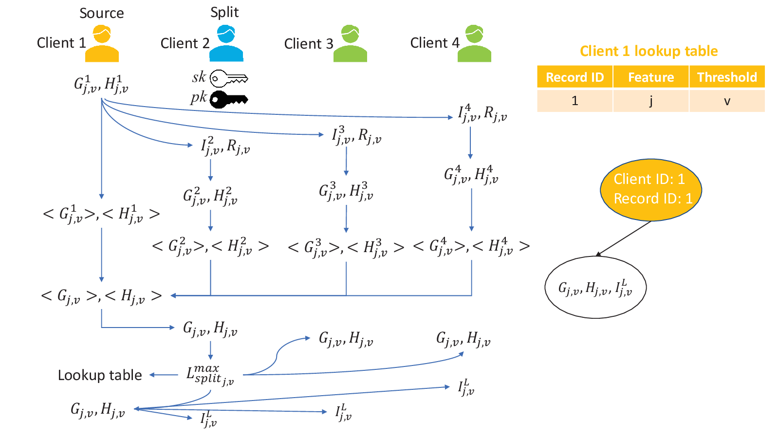
It is clear to see that above proposed secure node split protocol encrypts the intermediate summation values and for privacy concern and is able to effectively defend differential attacks. The source client contains all the split node IDs and their corresponding split features and thresholds. However, as shown in Fig. 4, the source client can only get the encrypted sum and for feature and threshold . Thus, differential attack does not work in this scenarios since only the split client has the secret key to get the plaintext and . On the other hand, the split client only knows local intersected data IDs and the final summation values and , but it has no idea of the corresponding data IDs. In addition, the split client only receive the temporary record number (this is just a arbitrary number defined by the source client, ’temporary’ means this number would be reset for the next node split) of the split and has no knowledge of the corresponding real split feature and threshold on the source client.
After all split clients decrypt and for all available features and threshold , they can calculate according to Eq. (4). In order to reduce both potential privacy leakage and communication costs, each split client compares and gets the largest value locally at first. The advantage of doing this is that each split client just needs to broadcast only one impurity score for comparison. If the current tree node continues splitting to the left branch as shown in Fig. 4, the split client needs to transmit the decrypted and to all other clients as and of the next tree node. In addition, the source client needs to send the data IDs of the left split to other clients. Therefore, each client can deduce the gradient and Hessian values from other clients through the received , and as discussed in Section III-C1. In order to alleviate this privacy leakage issue, we adopt a simple data instance threshold strategy. For example, if the number of received intersected data IDs is less than the pre-defined instance threshold, this client will reject to compute the local and this split will be removed during the node split. It should be mentioned that continue splitting is robust to differential attacks, since only one and are broadcast for each split. The overall secure node split protocol is also shown in Algorithm 2.
IV-B Construction of private tree nodes
After the split client with the largest impurity score is determined, will send the temporary record number of this split to the corresponding source client . And then the source client can add the feature and threshold with a unique record ID into the local lookup table [20], as shown in Fig. 4. After that, broadcasts the unique record ID to any other client that can annotate the split of current tree node with client ’s ID and the record ID.
Meanwhile, the source client can check and tell the split client whether the split child nodes are leaf or not based on the condition shown in line 5 and line 15 of Algorithm 3, respectively. If the child node is not leaf, the source client broadcasts the split data IDs and the split client broadcasts the corresponding summation of gradients and Hessian for continuing splitting the child node. If the child node is determined to be a leaf node, the split client computes the local leaf weight and stores it in a received lookup table with source client ID and record ID.
As a result, no client except the source client knows the feature and threshold of the tree node split, since the lookup table is stored locally without sharing with any other clients. And when it turns to new instance prediction, the source client needs to combine with the split client to get the leaf value. For instance, as shown a simple decision tree in Fig. 5, client is the source client of the root client and client is its corresponding split client. If a new data sample with age 30 and weight 150 comes for prediction, it will be sent to client for judgement. And then client uses its own lookup table to determine that this instance should go to the left branch (). After that, this data is sent to client to get its label prediction 0.41 (, go to right leaf). Also considering potential label leakage during data prediction for ensemble decision trees, we adopt secure aggregation scheme proposed in [13] for secure multi-party computation. Therefore, the final prediction for the data instance can be derived without revealing any leaf values.

IV-C Partial differential privacy
Suppose that the child node is a leaf node because training reaches either the maximum depth or the minimum node data samples. Then the leaf weight used for prediction will be calculated by split client (shown in line 5 and line 14 in Algorithm 3). There is no doubt that as the training proceeds, the accumulated label prediction will be closer to the true data label , and since the source client knows all the split data IDs, as long as it receives the leaf weight for prediction update, ’parts of’ 11 1 Here we call it ’parts of’, because XGboost is an ensemble tree algorithm. A client can get the real label predictions only if the leaf weights of all boosting trees of data samples are revealed to the client. the true labels of the corresponding data samples may have the risk of being revealed. However, all participating clients require the leaf value to update the corresponding local predictions. Thus, it is inevitable that will be sent to the source client, which means the source client has a potential opportunity to guess the true labels through the received .
In order to deal with this prediction update leakage issue, we propose a partial differential privacy (DP) mechanism, where the leaf value is perturbed with Gaussian noise before being sent to the source client. Since the calculation of the leaf value is based on the summation of and (the number of and is not fixed), its range is unknown beforehand. Before adding noise to the leaf values, we clip the leaf values and set the clip value as the sensitivity of differential privacy. The sensitivity of is calculated according to Eq. (9), where refers to the predefined clip value and are two sets, differing in one pair of and .
| (9) | ||||
By partial DP, we mean here that DP is apply on values that are sent to the source client only, since other clients only have the intersected local data IDs and have no idea about any other data IDs. The advantage of using this strategy is that the correct distributed label predictions can be achieved to the greatest extent, while preventing the source client from guessing the true labels. The details of the partial DP mechanism is presented in Algorithm 4:
IV-D Security analysis
Our proposed PIVODL framework avoids revealing both data features and labels on each participating client, and in this section, we will make a detailed security analysis of the leakage sources and protection strategies.
During the training process, each client sorts the data instances based on the features and their corresponding bucket thresholds which are stored privately on the local devices. In order to find the maximum impurity score , the source clients require the corresponding and from other clients, since labels are distributed on multiple clients. The true data labels can be deduced from the computed gradients .
Theorem 1.
Given a gradient , the true label of corresponding data point could be inferred.
Proof.
According to Eq. (2), adversarial attackers are able to infer the true labels of the -th data sample by if is known. ∎
To tackle this privacy issue, Paillier encryption is adopted in this work to encrypt all and for each bucket before sending them for summation aggregation. However, it is possible that the specific gradient information can still be inferred by a differential attack, if the clients have data ID information of its adjacent bucket splits.
Theorem 2.
There is still a high risk that the gradient of the -th data sample may be deduced with a differential attack, even if the intermediate and are encrypted.
Proof.
Assume and are two adjacent data sample sets for two possible splits that only differs in one data sample (or a few data samples). Although the client only knows the aggregated summation and , can be easily derived with a differential attack . ∎
Therefore, it is critical to ensure that the source client and split client perform the bucket split and aggregation separately. And then the source client only knows the data IDs of each feature split but has no knowledge of their corresponding summation values, the split client holds the summation values but does not know their data IDs.
Before building the next boosting tree, the predictions of all data samples need to be updated based on the corresponding leaf weights. It will not be surprising that the predicted labels are the same as the true labels as the training proceeds. Therefore, attackers can guess the correct labels with a high confidence level through the received leaf weights.
Theorem 3.
Given multiple boosting trees’ leaf values, it is possible to deduce the true labels of the corresponding data points.
Proof.
The label predictions in a classification problem can be calculated with equation , where refers to the learning rate, is the leaf weight of -th decision tree, and is the activation function. Therefore, once the source client knows parts of or even all the leaf values , the true labels have a high risk of being inferred. ∎
In order to address this issue, the split client applies the above-mentioned partial DP mechanism before sending the leaf values to the source client. In this way, we can reduce the risk for the source client to correctly guess the true labels from other clients.
V Experimental results
In this section, we first provide the experimental settings and then present the experimental results, followed by a discussion of the learning performance. After that, we evaluate the training time when implementing our privacy-preservation method. At the end, the communication cost and label prediction inference of PIVODL would be described.
V-A Experimental Settings
Three common public datasest are used in the experimental studies, where the first two are classification tasks and the third is a regression task.
Credit card [41]: It is a credit scoring dataset that aims to predict if a person will make payment on time. It contains in total 30,000 data samples with 23 features.
Bank marketing [42]: The data is related to direct marketing campaigns of a Portuguese banking institution. The prediction goal is to evaluate whether the client will subscribe a term deposit. It consists of 45211 instances and 17 features.
Appliances energy prediction [43]: It is a regression dataset of energy consumption in a low energy building, which has 19735 data instances and 29 attributes.
We partition each dataset into training data and test data. The training and test dataset occupies 80% and 20% of the entire data samples, respectively. Other experimental settings like the number of clients, the number of the maximum depth of the boosting tree are presented in Table II. Besides, each experiment is repeated for five times independently and the results of the mean values together with their standard deviations are plotted in the corresponding figures.
| Hyperparameters | Range | Default |
|---|---|---|
| Number of clients | [2,4,6,8,10] | 4 |
| Maximum depth | [2,3,4,5,6] | 3 |
| Number of trees | [2,3,4,5,6] | 5 |
| Learning rate | / | 0.3 |
| Regularization | / | 1 |
| Number of buckets | / | 32 |
| Encrypt key size | / | 512 |
| [2,4,6,8,10] | 8 | |
| Sensitivity clip | / | 2 |
| Sample threshold | / | 10 |
V-B Sensitivity analysis
Here, we empirically analyze the change of the learning performances as the number of participating clients, the maximum depth of the tree structure, the number of trees, and in the partial DP change. The results in terms of the mean, the best, and the worst performance over five independent runs are plotted in Fig. 6, 7, 8, and Fig. 9, respectively.
From the results, we can see that varying the number of clients does not affect the training performance very much, especially in the experiments without applying the partial DP. As shown in Fig. 6, it is clear to see that the test performances on these three datasets are relatively insensitive to different numbers of clients. These results make sense since non-parametric models trained in the VFL setting have nearly the same performance as those trained in the standard centralized learning [44]. By contrast, however, the average test accuracy on the Credit dataset drops from 0.82 to 0.8 when the number of clients is reduced to 2. And it is surprising to see that the root mean squared error (RMSE) on the test data of the Energy dataset with DP is slightly higher than those without DP over different number of clients. The reason for this is that the model may have overfit the training data without applying DP. For instance, when the number of clients is 4 (the default value), the training RMSE with DP is about 70.9, which is higher than that without DP (66.6). By contrast, the test RMSE with DP is approximately 0.8% lower than that without DP. Overall, the performances with DP and without DP are almost the same and the test performance degradation resulting from the DP is negligible. Besides, the performance of the proposed PIVODL algorithm is rather stable in different runs.


Fig. 7 shows the performance when varying the number of maximum depth of the boosting tree. For classification tasks, the accuracy is about 82 and 90 for Credit card and Bank marketing datasets, respectively. And test accuracy of these two datasets remains almost constant as the number of maximum depth increases, except that the results on the Credit dataset with DP have slight fluctuations when the number of maximum depth is 5. Moreover, it is easy to find that the performances with DP and without DP are almost the same, which shows that the impact of the partial DP on the model performance is negligible. On the regression task, the average RMSE decreases as the maximum depth increases, since more complex tree structures may have better model performance. Similar to the previous cases, the test performance with DP is better than that without DP because of over-fitting.


The performance change with the number of boosting trees is shown in Fig. 8. The results imply that only slight performance changes are observed when the number of boosting trees changes. On the Appliances energy prediction dataset, the RMSE slightly decreases with the increase in the number of boosting trees and the RMSE values with and without DP are nearly the same.


The test results on the three datasets over different values are shown in Fig.9. And it is surprising to see that the test performances on all three datasets have no clear changes with the decrease of the value. This is because the partial DP is applied only on part of predicted labels in the source client, which makes it very unlikely to influence the node split at the next level of node split. In addition, the split clients use de-noised leaf values for prediction during the test, which further reduces the performance biases caused by the proposed partial DP method.


V-C Evaluation on training time
In this section, we empirically analyze the training time affected by the number of participating clients, the number of maximum depth and the number of boosting trees. All the experiments are run on Intel Core i7-8700 CPU and the Paillier encryption system is implemented with the package in [45]. Just like what we did in the previous set of experiments, the mean values together with the best and worst performances out of five independent runs are included in the results of the ablation studies.
Fig. 10 shows the training time when varying the number of clients with and without encryption. In general, it consumes the least training time on the the bank marketing dataset since it has the smallest amount of data. When no parameter encryption is adopted, the training time of the three datasets almost keeps constant over different numbers of clients, which is consistent with the results reported in [20, 23]. The reason is that the data samples are partitioned across data features in VFL and setting different numbers of clients does not change the entire data entries. On the contrary, the training time with Paillier encryption increases linearly with the increase in the client numbers, since the amount of the encryption times is proportional to the number of clients in our proposed PIVODL algorithm.


The training times over different maximum depths of a boosting tree are shown in Fig. 11, and similarly, the cases with and without Paillier encryption are presented for comparison. The training time grows exponentially with the increasing maximum depth, and this phenomenon becomes more obvious with Pailler encryption is adopted. This makes sense since the computational complexity of one decision is , where is the maximum depth of the tree. More specifically, the training time on the Appliance energy prediction dataset for six different depths is about 2 and 5 minutes without and with encryption, respectively.


Fig. 12 indicates the training time consumption over different numbers of boosting trees. The training time increases linearly on the three datasets with increase in the number of boosting trees. Similar to the previous results, the time consumption when using Paillier encryption is much larger than that without encryption. For example, the runtime on the energy dataset for six boosting trees is approximately 800 seconds with encryption, while it takes only about 350 seconds without encryption.


V-D Evaluation on communication cost
In this section, we empirically analyze the communication costs (in MB) affected by the number of participating clients, the number of the maximum depth and the number of boosting trees.
Communication costs are measured by varying the number of clients for both cases with and without using Paillier encryption. As shown in Fig. 13, the total communication costs for the three datasets increase with the number of clients. More specifically, the communication costs go up dramatically from two clients to four clients, and then increase relatively slightly from four clients to ten clients. Different from the results on the training time, the communication costs with Paillier encryption increase but not as much as the computation time compared to the cases without encryption. This can be attributed to the fact that it is unnecessary to transmit the ciphertexts of the gradients and Hessian values of each data sample for all possible node splits, and only the ciphertexts of the intermediate summation values are required for transmission (see line 27 in Algorithm 2).


Fig. 14 shows the communication costs over different maximum depths with and without Paillier encryption. It is apparent to see that the communication costs are proportional to the maximum depth in both encryption and non -encryption scenarios. The communication costs are similar for the three datasets when the maximum depth is two, and they grow almost linearly with increase in the tree depth. The communication costs of the Appliances energy prediction dataset are 290MB without encryption and 425MB with encryption for a depth of six, which is the largest among all the three datasets.


The communication costs related to the number of boosting trees are shown in Fig .15. Similar to the previous results, the communication costs increase linearly with the number of trees, since the model size of XGBoost is proportional to the number of trees. And it is clear to see that the impact of encryption on communication costs is not as significant as that on the training time. The encryption brings a maximum of 25MB extra communication costs for the model with six boosting trees on the Appliance energy prediction dataset.


V-E Inference of predicted labels
In this section, we assume that each client is curious but honest and attempts to deduce the true label information of other clients through the available leaf weights. The attack strategy is, for instance, to ensemble all the leaf values and guess a label if one client knows several leaf values of one specific data sample. By comparing the ’guessed’ labels with the true labels from other clients, it is easy to calculate the guess accuracy of each client. Note that for a binary classification problem, the data labels are either 0 or 1 and the probability of a correct random guess is 50%. Therefore, if the guess accuracy is equal to or less than 50%, the label privacy is not revealed.
|
|
|
|
|
|
| |||||||||||||||||||
|---|---|---|---|---|---|---|---|---|---|---|---|---|---|---|---|---|---|---|---|---|---|---|---|---|---|
|
68.75% | 30.02% | 23.02% | 34.15% | 27.78% | 40.93% | |||||||||||||||||||
|
61.57% | 39.57% | 38.85% | 25.85% | 39.73% | 14.45% |
For the sake of brevity, we calculate the expected guess accuracy of all participating clients with and without partial DP using different values. As shown in Table III, the guess accuracy is more than 60% for both two datasets without using partial DP, which is more accurate than a random guess. After applying the proposed partial DP algorithm, however, the guess accuracies drop dramatically and are all less than 50%. Specifically on the Credit card dataset, the guess accuracy decreases to around 27% for and 45% for . On the Bank marketing dataset, the guess accuracy drops to 14.45 when . Since the noise in the DP follows the Gaussian distribution, it is normal that a smaller values will give a higher guess accuracy. But as long as partial DP is used for label privacy protection, the guess accuracy is lower than a random guess, meaning that no label privacy is leaked from the received leaf outputs.
VI Conclusion and future work
In this paper, we propose a secure learning system, called PIVODL, for privately training XGBoost decision tree models in a vertical federated learning environment with labels distributed on multiple clients. A secure node split protocol and a privacy-preserving tree training algorithm are proposed by requiring the source and split clients to separately split the data samples and calculate the corresponding impurity scores, effectively defending against differential attacks that may be encountered during the boosting tree node splits. In addition, a partial DP mechanism is adopted to deal with label privacy so that no client is able to guess the correct data labels through the revealed leaf weights.
Our experimental results empirically indicate that the proposed PIVODL framework is able to securely construct ensemble trees with negligible performance degradation. We show the test performance of the resulting decision trees is relatively insensitive to different values of the introduced DP, since the proposed algorithm adds Gaussian noise only to the leaf weights that are sent to the source clients. Moreover, the partial DP can effectively prevent labels of the data from being revealed through the received leaf weights.
Although the proposed PIVODL system shows promising performance in VFL, improving training efficiency remains challenging. The encryption in PIVODL still takes a large proportion of both learning time and communication costs. Therefore, our future work will be dedicated to developing a light weighted and efficient secure XGBoost system for VFL with labels distributed on multiple devices.
References
- [1] B. McMahan, E. Moore, D. Ramage, S. Hampson, and B. A. y Arcas, “Communication-efficient learning of deep networks from decentralized data,” in Artificial Intelligence and Statistics, pp. 1273–1282, PMLR, 2017.
- [2] Q. Yang, Y. Liu, T. Chen, and Y. Tong, “Federated machine learning: Concept and applications,” ACM Trans. Intell. Syst. Technol., vol. 10, Jan. 2019.
- [3] L. T. Phong, Y. Aono, T. Hayashi, L. Wang, and S. Moriai, “Privacy-preserving deep learning via additively homomorphic encryption,” IEEE Transactions on Information Forensics and Security, vol. 13, no. 5, pp. 1333–1345, 2018.
- [4] S. Truex, N. Baracaldo, A. Anwar, T. Steinke, H. Ludwig, R. Zhang, and Y. Zhou, “A hybrid approach to privacy-preserving federated learning,” in Proceedings of the 12th ACM Workshop on Artificial Intelligence and Security, AISec’19, (New York, NY, USA), p. 1–11, Association for Computing Machinery, 2019.
- [5] R. Xu, N. Baracaldo, Y. Zhou, A. Anwar, and H. Ludwig, “Hybridalpha: An efficient approach for privacy-preserving federated learning,” in Proceedings of the 12th ACM Workshop on Artificial Intelligence and Security, AISec’19, (New York, NY, USA), p. 13–23, Association for Computing Machinery, 2019.
- [6] C. Zhang, S. Li, J. Xia, W. Wang, F. Yan, and Y. Liu, “Batchcrypt: Efficient homomorphic encryption for cross-silo federated learning,” in 2020 USENIX Annual Technical Conference (USENIX ATC 20), pp. 493–506, USENIX Association, July 2020.
- [7] H. Zhu, R. Wang, Y. Jin, K. Liang, and J. Ning, “Distributed additive encryption and quantization for privacy preserving federated deep learning,” arXiv preprint arXiv:2011.12623, 2020.
- [8] R. Shokri and V. Shmatikov, “Privacy-preserving deep learning,” in Proceedings of the 22nd ACM SIGSAC Conference on Computer and Communications Security, CCS ’15, (New York, NY, USA), p. 1310–1321, Association for Computing Machinery, 2015.
- [9] T. Orekondy, S. J. Oh, Y. Zhang, B. Schiele, and M. Fritz, “Gradient-leaks: Understanding and controlling deanonymization in federated learning,” in NeurIPS Workshop on Federated Learning for Data Privacy and Confidentiality, 2019.
- [10] J. Geiping, H. Bauermeister, H. Dröge, and M. Moeller, “Inverting gradients - how easy is it to break privacy in federated learning?,” in Advances in Neural Information Processing Systems (H. Larochelle, M. Ranzato, R. Hadsell, M. F. Balcan, and H. Lin, eds.), vol. 33, pp. 16937–16947, Curran Associates, Inc., 2020.
- [11] H. Li and T. Han, “An end-to-end encrypted neural network for gradient updates transmission in federated learning,” arXiv preprint arXiv:1908.08340, 2019.
- [12] O. Goldreich, “Secure multi-party computation,” Manuscript. Preliminary version, vol. 78, 1998.
- [13] K. Bonawitz, V. Ivanov, B. Kreuter, A. Marcedone, H. B. McMahan, S. Patel, D. Ramage, A. Segal, and K. Seth, “Practical secure aggregation for privacy-preserving machine learning,” in Proceedings of the 2017 ACM SIGSAC Conference on Computer and Communications Security, CCS ’17, (New York, NY, USA), p. 1175–1191, Association for Computing Machinery, 2017.
- [14] C. Gentry et al., A fully homomorphic encryption scheme, vol. 20. Stanford university Stanford, 2009.
- [15] C. Dwork, “Differential privacy: A survey of results,” in Theory and Applications of Models of Computation (M. Agrawal, D. Du, Z. Duan, and A. Li, eds.), (Berlin, Heidelberg), pp. 1–19, Springer Berlin Heidelberg, 2008.
- [16] S. Hardy, W. Henecka, H. Ivey-Law, R. Nock, G. Patrini, G. Smith, and B. Thorne, “Private federated learning on vertically partitioned data via entity resolution and additively homomorphic encryption,” arXiv preprint arXiv:1711.10677, 2017.
- [17] R. Nock, S. Hardy, W. Henecka, H. Ivey-Law, G. Patrini, G. Smith, and B. Thorne, “Entity resolution and federated learning get a federated resolution,” arXiv preprint arXiv:1803.04035, 2018.
- [18] Y. Liu, X. Zhang, and L. Wang, “Asymmetrically vertical federated learning,” arXiv preprint arXiv:2004.07427, 2020.
- [19] S. Yang, B. Ren, X. Zhou, and L. Liu, “Parallel distributed logistic regression for vertical federated learning without third-party coordinator,” arXiv preprint arXiv:1911.09824, 2019.
- [20] K. Cheng, T. Fan, Y. Jin, Y. Liu, T. Chen, D. Papadopoulos, and Q. Yang, “Secureboost: A lossless federated learning framework,” 2021.
- [21] T. Chen and C. Guestrin, “Xgboost: A scalable tree boosting system,” in Proceedings of the 22nd ACM SIGKDD International Conference on Knowledge Discovery and Data Mining, KDD ’16, (New York, NY, USA), p. 785–794, Association for Computing Machinery, 2016.
- [22] Y. Wu, S. Cai, X. Xiao, G. Chen, and B. C. Ooi, “Privacy preserving vertical federated learning for tree-based models,” Proc. VLDB Endow., vol. 13, p. 2090–2103, July 2020.
- [23] Z. Tian, R. Zhang, X. Hou, J. Liu, and K. Ren, “Federboost: Private federated learning for gbdt,” 2020.
- [24] Q. Yang, Y. Liu, T. Chen, and Y. Tong, “Federated machine learning: Concept and applications,” ACM Transactions on Intelligent Systems and Technology (TIST), vol. 10, no. 2, pp. 1–19, 2019.
- [25] Y. Liu, Y. Kang, L. Li, X. Zhang, Y. Cheng, T. Chen, M. Hong, and Q. Yang, “A communication efficient vertical federated learning framework,” Unknown Journal, 2019.
- [26] M. Isard, M. Budiu, Y. Yu, A. Birrell, and D. Fetterly, “Dryad: distributed data-parallel programs from sequential building blocks,” in Proceedings of the 2nd ACM SIGOPS/EuroSys European Conference on Computer Systems 2007, pp. 59–72, 2007.
- [27] M. Isard and Y. Yu, “Distributed data-parallel computing using a high-level programming language,” in Proceedings of the 2009 ACM SIGMOD International Conference on Management of data, pp. 987–994, 2009.
- [28] Y. Y. M. I. D. Fetterly, M. Budiu, Ú. Erlingsson, and P. K. G. J. Currey, “Dryadlinq: A system for general-purpose distributed data-parallel computing using a high-level language,” Proc. LSDS-IR, vol. 8, 2009.
- [29] D. W. Hosmer Jr, S. Lemeshow, and R. X. Sturdivant, Applied logistic regression, vol. 398. John Wiley & Sons, 2013.
- [30] I. Goodfellow, Y. Bengio, A. Courville, and Y. Bengio, Deep learning, vol. 1. MIT press Cambridge, 2016.
- [31] Y. LeCun, Y. Bengio, and G. Hinton, “Deep learning,” nature, vol. 521, no. 7553, pp. 436–444, 2015.
- [32] T. ElGamal, “A public key cryptosystem and a signature scheme based on discrete logarithms,” IEEE Transactions on Information Theory, vol. 31, no. 4, pp. 469–472, 1985.
- [33] P. Paillier, “Public-key cryptosystems based on composite degree residuosity classes,” in TAMC, Springer, 1999.
- [34] C. Dwork, F. McSherry, K. Nissim, and A. Smith, “Calibrating noise to sensitivity in private data analysis,” in Theory of cryptography conference, pp. 265–284, Springer, 2006.
- [35] C. Dwork, K. Kenthapadi, F. McSherry, I. Mironov, and M. Naor, “Our data, ourselves: Privacy via distributed noise generation,” in Annual International Conference on the Theory and Applications of Cryptographic Techniques, pp. 486–503, Springer, 2006.
- [36] M. Abadi, A. Chu, I. Goodfellow, H. B. McMahan, I. Mironov, K. Talwar, and L. Zhang, “Deep learning with differential privacy,” in Proceedings of the 2016 ACM SIGSAC conference on computer and communications security, pp. 308–318, 2016.
- [37] K. Wei, J. Li, M. Ding, C. Ma, H. H. Yang, F. Farokhi, S. Jin, T. Q. S. Quek, and H. V. Poor, “Federated learning with differential privacy: Algorithms and performance analysis,” IEEE Transactions on Information Forensics and Security, vol. 15, pp. 3454–3469, 2020.
- [38] R. C. Geyer, T. Klein, and M. Nabi, “Differentially private federated learning: A client level perspective,” arXiv preprint arXiv:1712.07557, 2017.
- [39] V. Kolesnikov, N. Matania, B. Pinkas, M. Rosulek, and N. Trieu, “Practical multi-party private set intersection from symmetric-key techniques,” in Proceedings of the 2017 ACM SIGSAC Conference on Computer and Communications Security, pp. 1257–1272, 2017.
- [40] B. Pinkas, T. Schneider, and M. Zohner, “Faster private set intersection based on OT extension,” in 23rd USENIX Security Symposium (USENIX Security 14), pp. 797–812, 2014.
- [41] I.-C. Yeh and C.-h. Lien, “The comparisons of data mining techniques for the predictive accuracy of probability of default of credit card clients,” Expert Systems with Applications, vol. 36, no. 2, pp. 2473–2480, 2009.
- [42] S. Moro, P. Cortez, and P. Rita, “A data-driven approach to predict the success of bank telemarketing,” Decision Support Systems, vol. 62, pp. 22–31, 2014.
- [43] L. M. Candanedo, V. Feldheim, and D. Deramaix, “Data driven prediction models of energy use of appliances in a low-energy house,” Energy and buildings, vol. 140, pp. 81–97, 2017.
- [44] H. Zhu, J. Xu, S. Liu, and Y. Jin, “Federated learning on non-iid data: A survey,” arXiv preprint arXiv:2106.06843, 2021.
- [45] C. Data61, “Python paillier library.” https://github.com/data61/python-paillier, 2013.