A Historical Perspective of Adaptive Control and Learning
Thanks: The first author is supported by the Boeing Strategic University Initiative. The second author performed his part of the work in IPME RAS under support by Ministry of Science and Higher Education of the Russian Federation (Project no. 075- 15-2021-573 ).
Published at https://doi.org/10.1016/j.arcontrol.2021.10.014.
Abstract
This article provides a historical perspective of the field of adaptive control over the past seven decades and its intersection with learning. A chronology of key events over this large time-span, problem statements that the field has focused on, and key solutions are presented. Fundamental results related to stability and robustness of adaptive systems and learning of unknown parameters are sketched. A brief description of various applications of adaptive control reported over this period is included.
1 Introduction
The goal of adaptive control is real-time control of uncertain dynamic systems through adaptation and learning. This paper takes a historical perspective of the field of adaptive control over the past seven decades. Given the recent upsurge of interest in learning, in the Machine Learning and Control communities, both offline and online, such a perspective is timely and warranted.
The scope that we aim to cover is clearly ambitious. Covering events that span 70 years, chronicled in more than 15 textbooks, 20 edited books, hundreds of surveys, and thousands of research publications in journals and conferences in 30 pages is a formidable task. The goal of this article is to accomplish this task by focusing on the highlights of this field, emphasize key lessons learned, delineate key solutions derived, and identify a few takeaway messages.
Here are the highlights of this article:
- •
Over the last seventy years, the field of adaptive control has witnessed advances in both deterministic and continuous-time systems and stochastic discrete-time systems. This article is one of the first attempts to trace the development in both domains.
- •
The article focuses mainly on those advances in adaptive control that have a significant intersection with parameter learning.
- •
This article has made a concerted effort in chronicling key advances that have occurred globally.
- •
The article presents events chronologically (Section II), through problem statements (Section III), and through highlights of solutions (Section IV). An interested reader may delve into only one or more of these sections and do a deeper dive, if interested, by reading any of the 250 references listed at the end of the article.
- •
The article provides a snapshot of various applications of adaptive control (Section V).
- •
Concluding remarks including a few takeaway messages are provided in Section VI.
When it comes to real-time control of uncertain dynamic systems, the efforts of the control community extend significantly beyond adaptive control. There are several topics that are at the boundaries, such as sliding-mode control, iterative learning control, and linear-parameter-varying control that are not addressed in this survey. While we devote a section to the topic of reinforcement learning (RL) that has a rich intersection and complementarity to adaptive control, we defer the reader to other articles for a more comprehensive discussion on RL as well as other topics that lie at the intersection of adaptation and learning.
2 A chronology
The history of adaptive control systems is almost as long as the entire field of control systems, as the concept of adaptation is fairly close to the notion of feedback. As such, this concept has been explored from the 1950s to the present and continues to be an area of intense activity. We classify various developments in this area into three chunks of time, 1950-65, 1965-85, and 1990s-2000. During the first 15 years, several contributions arose separately in the context of deterministic continuous-time systems and pattern-recognition (which employed a stochastic framework), and are organized under these two broad headings. Subsequent sections outline parallel developments in deterministic and stochastic systems in a combined manner. While the 70s and 80s witnessed the development of a stability framework, later decades developed a robustness framework for the adaptive systems. Key developments in all of these decades are outlined below.
2.1 1950-65
2.1.1 Deterministic and continuous time
The term adaptation is defined in biology as “an advantageous conformation of an organism to changes in its environment.” The earliest reflection of this principle in an engineering context can be found in (Drenick and Shahbender 1957)11 1 Origins of adaptation rules can be traced even earlier to 1949, in the form of Hebbian rules (Hebb 1949) that connected weight adjustments in a neuron to performance.. The authors coopted this fundamental principle in their definition of an adaptive system in the context of a control system, and defined an adaptive control system to be one which monitored its own performance and adjusted its parameters in the direction of better performance Drenick and Shahbender 1957. The implicit implication here is that a non-adaptive system would then have parameters that are fixed and not adjusted. To provide more clarity, and distinguish an adaptive system from a non-adaptive one, references Aseltine et al. 1958 and Stromer 1959 introduced definitions of adaptive systems. In fact, there was a profusion of definitions of adaptive systems at this time based on what was adapted, what the adaptation was in response to, time-scales of adaptation, or from whose viewpoint. It could be argued that the classes of adaptive systems outlined in (Aseltine et al. 1958) are precursors to the current approaches in adaptive control.
Similar to Drenick and Shahbender 1957, the authors of Whitaker et al. 1958 focused on a servo problem where the process output was required to follow a commanded output in the presence of parametric uncertainties. They developed what came to be known as the MIT-rule as a core adaptive mechanism which served as an outer loop with the inner loop consisting of a standard feedback control system. The adaptive mechanism adjusted the control parameter using a simple rule
| (1) |
where denoted a tracking error between the process output and a reference output , and stands for the gradient. The idea therefore is to have the adaptive mechanism use (1) to estimate, i.e. learn the correct value of the parameter that the feedback controller in the inner loop must deploy. This main idea continues to pervade all adaptive control methods to-date.
The motivation for the study and implementation of adaptive control systems came from applications in aerospace – for autopilot design in flight control (Gregory 1959; Hammond 2013). As high performance aircraft routinely encounter a wide range of operating conditions, there was a need to develop sophisticated regulators that would adapt their parameters online so that they are not constrained to work with constant gains which may limit their operation to a small flight envelope. This led to several symposia on adaptive systems in the early 60s, with what was referred to as a three-legged milking stool for advanced flight control systems that consisted of aerodynamics, GNC (Guidance, Navigation, and Control), and adaptation (Hammond 2013). Around the same time, Bellman and Kalaba introduced the term adaptive in the context of multistage decision processes as belonging to the last of a series of three stages in the evolution of control processes. With the first two denoted as deterministic and stochastic control processes, an adaptive control process was defined as when the designer has very little knowledge about the system dynamics or even the statistics of any random inputs that may be present (Bellman and Kalaba 1959; Bellman 2015). Yet another early evidence of interest in adaptive regulators is a patent by Caldwell (Caldwell 1950). Several additional references can be found in Astrom 1996 and in Chapter 1 in Narendra and Annaswamy 2005.
Cautionary inputs and guidance for the design of the controllers and the adaptive mechanisms soon started to appear. Any successful adaptive system has to cope with changes in its environment for its survival and performance. Familiarity with the environment results in better understanding, and better understanding enables the system to better predict the changes in the system. However, understanding and controlling are two distinct activities; predictive ability does not translate directly into the ability to control. Often the converse may be true – a better ability to control may help in a better understanding but here too there may be limits. Needless to say, the connection between identification and control is complex and was explored in a number of seminal papers and textbooks during the ’60s. One of them is Feldbaum’s concept of dual control (Feldbaum 1960b), that emphasized the need for an optimal control action that is taken for a system with uncertainties. Feldbaum pointed out that the requisite control has to have dual components, one of probing for enhancing identification and one of caution for ensuring stable control action. Too much of a focus on identification may not result in satisfactory control; too much emphasis on controlling the system may not lead to satisfactory learning. The design of dual control with the right mix of both of these components is therefore a huge challenge and the grand goal of the field of adaptive control. These two intertwined concepts of identification and control pervade Machine Learning (ML) as well (Kaelbling et al. 1996; Ishii et al. 2002), and often go under the monikers of “exploration” and “exploitation.”
2.1.2 Pattern Recognition and Classification
A parallel development of adaptation can be traced in the field of pattern recognition and classification, which occurred during the same period. As the title of Widrow 1964 attests, it was observed that a gradient descent type algorithm, similar to that in (1), plays a central role not only in control problems but also in pattern recognition. In addition to (Widrow 1961; Widrow 1964; Abramson et al. 1963), several groups in USSR led by Aizerman Aizerman 1963, Lerner Vapnik and Lerner 1963; Vapnik and Chervonenkis 1964, Yakubovich V.A.Yakubovich 1963; V.A.Yakubovich 1965, and others (Bongard 1961; Braverman 1962; Fradkov 2020; Fradkov and Polyak 2020) developed deterministic and stochastic approaches for input classification and pattern recognition. A common element to a diverse set of problems in pattern recognition, signal processing (Widrow et al. 1967), and perceptrons (Rosenblatt 1961), was the determination of a set of parameters or weights that leads to desired classification, filtering, or tracking performance using input-output data. In contrast to the earlier discussions of control systems, the treatment in these works was in discrete-time rather than continuous time, and instead of a deterministic framework, employed a stochastic framework with noisy measurements and inputs. Widrow’s Adaline filters also led to the foundation of neural networks, deep and otherwise (Widrow and Lehr 1990). The approach taken in many of these works was statistical in nature, with their foundations in communications and decision theory (Marill and Green 1960; Widrow 1960). Except for brief mentions, this survey will not focus on the evolution of pattern recognition or its intersection with adaptive control.
2.2 1965-1985
It was soon realized that the MIT-rule proposed in Whitaker et al. 1958 can result in instability, especially when there is sufficient phase lag between the measurement of error and adjustment of the parameters. Several authors contributed to the formulation of a stability framework for the analysis and synthesis of adaptive systems where real-time decisions in the form of parameter adjustment in dynamic systems were taken using online data. Notable ones came from the authors of Grayson 1963, Shackcloth and Butchart 1965, Parks 1966, Monopoli 1967, and Narendra and Kudva 1974. Lyapunov’s method was suggested in lieu of a gradient descent approach as in (1), and ended up as the foundation for stability of adaptive systems22 2 In hindsight, the MIT-rule can be viewed as a partial Lyapunov function, as it only included an -norm of the performance error in its cost function.. Independently, the same problem with similar conceptual tradeoffs was also addressed in deterministic discrete time setting by Yakubovich in V.A.Yakubovich 1968; V.A.Yakubovich 1972. Several seminal results were published during this period which witnessed surveys by Lindorff and Carroll (Lindorff and Carroll 1973), Landau (Landau 1974), Wittenmark (Wittenmark 1975), Unbehauen (Unbehauen et al. 1975), and others (Asher et al. 1976; Parks et al. 1980; Voronov and Rutkovsky 1984). These were followed by edited books such as Narendra 1980 (reprinted 2012; Unbehauen 1980; Harris 1981, and subsequent textbooks in deterministic and continuous-time Fomin et al. 1981; Narendra and Annaswamy 1989; Åström and Wittenmark 1995; Ioannou and Sun 1996; Sastry and Bodson 1989; Tao 2003; Krstić et al. 1995; Fradkov et al. 1999, stochastic systems in books and papers such as Kumar and Varaiya 1986; Duncan and Pasik-Duncan 1990; Borkar and Varaiya 1979; Becker et al. 1985; Fomin 1991, and multiple-input, multiple-output systems in Tao 2003. These addressed adaptive control architectures and algorithms for a range of dynamic systems, with either full-state or partial-state measurements available in real-time. The efforts during these 15 years laid the foundation for stable adaptation in dynamic systems, both deterministic and stochastic, where the uncertainties were predominantly in their parameters. The overall goal was to ensure a closed-loop system that was well-behaved and met control goals such as tracking and regulation asymptotically.
In deterministic systems, the structure of the algorithm for adjusting their parameter was of the form
| (2) |
where is a suitably chosen regressor that may or may not coincide with the gradient of a well-defined loss function, and represents a normalization component. The choices of and were guided by the determination of an underlying Lyapunov function and the interplay between the adjustable parameters and the signals in the closed-loop system, leading to an approach that is most commonly termed Model Reference Adaptive Control (MRAC) and used in deterministic continuous-time systems. In stochastic systems, the works by Astrom and coworkers (Astrom and Wittenmark 1973; Åström and Wittenmark 1995) led to Self-tuning Regulators (STR) associated with minimum variance controller with their foundation laid in papers such as (Ljung 1977b),(Solo 1979; Landau 1982; Bitmead 1983; Kumar 1983; Clarke et al. 1985; Johansson 1995). In all these cases, conditions under which learning, that is, accurate parameter estimation, can take place were precisely articulated. Both necessary and sufficient conditions were derived (Morgan and Narendra 1977; Ljung 1977a; Ljung 1977b; Ljung and Söderström 1983; Anderson 1985).
Yet another link between adaptation and learning is due to Yakov Tsypkin who proposed a unified framework based on stochastic approximation machinery. Parameter choice and convergence results then follow from the results on stochastic approximation obtained earlier in mathematical statistics based on average risk minimization (Tsypkin 1966; Tsypkin 1968). We defer the details of the problem statement to Section III.
As evidenced by the chronology above, there are two parallel, and very similar evolution of the branches of adaptive control in deterministic systems and stochastic systems, with the obvious distinction associated with the underlying tools. The problem of convergence of the tracking error in the former case had a counter-part of a minimum variance controller in the latter. The term adaptive controller remained in vogue for deterministic systems and its counterpart in stochastic systems was termed self-tuning regulators; the terms adaptation and self-tuning were used synonymously. The fundamental tenets of stability and convergence in adaptive systems and tradeoffs between performance and learning were however found to be invariant to these two branches. We note that for stochastic systems, our focus in this paper is restricted to adaptation and parameter learning in discrete-time systems. There is a significant and rich literature present in adaptive control of stochastic continuous-time systems as well (see Wertz et al. 1989; Gevers et al. 1991; Caines 1992; Duncan et al. 1999 for linear systems and Li and Krstic 2020 for nonlinear systems). Most of these ideas and results have discrete-time counterparts, which are presented in brief in the following sections. Details of the problem statements are postponed until section III.
2.3 1990s-present
2.3.1 Adaptive Control of Deterministic and Stochastic Systems
With the stability framework established in the 70s, the next broad milestone in the evolution of adaptive control systems was a robustness framework established in the 80s with textbooks capturing the details of various solutions in the 90s. It was soon realized that both gradient algorithms as in (1) and stability-based algorithms that employed a Lyapunov approach as in (2) were inadequate in ensuring robustness to perturbations such as bounded disturbances and unmodeled dynamics (Rohrs et al. 1982). Several approaches were developed around the same time (Egardt 1979; Peterson and Narendra 1982; Kreisselmeier and Narendra 1982; Ioannou and Kokotovic 1984; Praly 1984b; Praly 1984a; Anderson et al. 1986; Narendra and Annaswamy 1986; Narendra and Annaswamy 1987a; Ioannou and Tsakalis 1986a; Middleton and Goodwin 1988; Tsakalis and Ioannou 1989; Ortega and Tang 1989; Naik et al. 1992) in ensuring that adaptive control systems not only provided appropriate adaptation to accommodate parametric uncertainties but also provided robustness to withstand non-parametric uncertainties such as external disturbances, time-varying parameters, and unmodeled dynamics. Broadly, these approaches either relied on properties of persistent excitation of the exogenous command signals (Anderson et al. 1986; Narendra and Annaswamy 1986) with the same adaptive laws as in (2), or in modifying the adaptive law in a suitable manner (Fradkov 1980; Peterson and Narendra 1982; Kreisselmeier and Narendra 1982; Ioannou and Tsakalis 1986a; Narendra and Annaswamy 1987a; Fradkov 1987; Wen and Hill 1992). A parallel to the latter corresponds to the use of regularization in machine learning (Gaudio et al. 2020b). Similar results can be found in discrete time as well (for example, (Ioannou and Tsakalis 1986b; Tao and Kokotović 1995; Wen and Hill 1992; Cluett et al. 1988)). The use of diminished persistent excitation with time was utilized to obtain an elegant framework for adaptive optimal control in stochastic systems in (Guo and Chen 1991; Guo 1995; Duncan et al. 1999).
The above stability and robustness arguments also set the stage for addressing the control of nonlinear systems with parametric uncertainties. This too was addressed starting in the 90s, spawning a huge area of research with dozens of researchers laying the foundation of key results (see for example Krstić et al. 1995). Special classes of adaptive nonlinear systems that arise in robotics were addressed at length in Slotine and Li 1991 even earlier. Methods based on feedback linearization, backstepping, and averaging led to several seminal results in this area. A class of problems related to control of nonlinear systems using neural networks witnessed significant activity during this period as well (see for example, Narendra and Parthasarathy 1991; Sanner and Slotine 1992; Rovithakis and Christodoulou 1994; Polycarpou 1996; Yu and Annaswamy 1996; Yu and Annaswamy 1998; Lavretsky and Hovakimyan 2008; Ren et al. 2010a).
2.3.2 Reinforcement learning/Approximate Dynamic Programming
Towards the end of the 1980s the approach of reinforcement learning (Sutton and Barto 2018; Kaelbling et al. 1996) was formulated and in the early 1990s strong ties were identified between these topics and adaptive optimal control. A case in point is the reference Sutton et al. 1992, clearly indicated in its title, Reinforcement learning is direct adaptive optimal control. In the works on control based on RL, a performance index is introduced, usually as an integral functional, and neural networks are used to approximate either the predicted optimal value (Bellman function) of this functional (known as Value Iteration (VI)) or the optimal control policy (policy iteration), based on the HJB equation. Such an approach is referred to as “approximate dynamic programming”, ”neuro dynamic programming” (Powell 2007; Bertsekas 2008), or “adaptive dynamic programming” (Lewis and Vrabie 2009). Analytical frameworks for cases when the state and action sets are finite and for the more difficult case when they are infinite have been addressed. Related problem statements are briefly addressed in Section III.
3 Problem Statements
This section outlines the problem statements that have been proposed under the rubric of adaptive control. We classify them into four categories, the first three of which are based on whether they are in continuous-time or discrete-time, and deterministic or stochastic. We do not address stochastic continuous-time systems in this paper mostly since that area was developed much in parallel with the discrete-time case (Wertz et al. 1989; Gevers et al. 1991; Caines 1992; Duncan et al. 1999; Li and Krstic 2020). A brief discussion on RL is also included in this section.
3.1 Deterministic and Continuous-time Systems
The aim in adaptive control problems is to design an exogenous input that affects the dynamics of a system given by
| (3) |
where represents the system state, represents all measurable system outputs, with many physical systems obeying the inequality (Qu et al. 2020). represents system parameters that may be unknown, and and denote system dynamics, that may be nonlinear, that capture the underlying physics of the system. The functions and also vary with , as disturbances (often modeled as deterministic quantities) and stochastic noise may affect the states and output. The goal is to choose so that tracks a desired command signal at all , and so that an underlying cost is minimized. In what follows, we will refer to the system that is being controlled as a plant.
As the description of the system as in (3) is based on a plant model, and as the goal is to determine the control input in real time, all control approaches make assumptions regarding what is known and unknown. To begin with, as the plant is subject to various perturbations and modeling errors due to environmental changes, complexities in the underlying mechanisms, aging, and anomalies, both and are not fully known. The field of adaptive control has taken a parametric approach to distinguish the known parts from the unknown. In particular, it is assumed that is a known function, while the parameter is unknown. A real time control input is then designed so as to ensure that the tracking goals are achieved by including an adaptive component that attempts to estimate the parameters online. A linearized version of the problem in (3) is of the form
| (4) |
where denotes the differential operator , is a rational operator of , and is an unknown parameter, and the goals of tracking and regulation are the same as above.
In the following subsections, four broad categories of subproblems that have been addressed in the context of adaptive control in deterministic continuous-time systems are described.
3.1.1 Boundedness and real-time decision making
As mentioned above, the control goal is to ensure that
| (5) |
where . As these decisions are required to be made in real time, the focus of the solutions is to have them lead to a closed-loop dynamic system that has bounded solutions at all time and a desired asymptotic behavior. The central question, therefore, is if this can be ensured even when there are parametric uncertainties in and several other non-parametric uncertainties that may due to unmodeled dynamics, disturbances, and the like. Once this is guaranteed, the question of learning, in the form of parameter convergence, is addressed. As a result, control for learning is a central question that is pursued in the class of problems addressed in adaptive control rather than learning for control (Krstic 2021).
3.1.2 Certainty Equivalence Principle and Adaptive Control Solutions
The well known certainty equivalence principle (CEP) proceeds with the following mantra: first, optimize under perfect foresight, then substitute optimal estimates for unknown values. This philosophy underlies all adaptive control solutions by first determining a controller structure that leads to an optimal solution when the parameters are known and then replace the parameters in the controller with their estimates. The difficulty in adopting this philosophy to its fullest stems from the dual nature of the adaptive controller, as it attempts to accomplish two tasks simultaneously, estimation and control. This simultaneous action introduces a strong nonlinearity into the picture and therefore renders a true deployment of the certainty equivalence principle difficult if not impossible. The procedure for adaptive control is therefore modified, with the first step corresponding to a controller that leads to a stable solution rather than optimal one. In other words, much of the adaptive control literature has focused on deriving stable solutions first and foremost for the real-time control of systems with parametric uncertainties, followed by an effort to estimate the unknown parameters, and optimization addressed at the final step. Such a breakdown of the problem overcomes the intractability of the certainty equivalence principle and leads to tractable procedures.
A typical solution of the adaptive controller takes the form
| (6) | |||||
| (7) |
where is an estimate of a control parameter that is intentionally varied as a function of time, represents all available data at time . The nonautonomous nature of is due to the presence of exogenous signals such as set points and command signals. The functions and are deterministic constructions, and make the overall closed-loop system nonlinear and nonautonomous. The challenge is to suitably construct functions and so as to have learn the requisite unknown control parameter , and ensure that stability and asymptotic stability properties of the overall adaptive systems are ensured. These constructions have been delineated for deterministic systems in (Narendra and Annaswamy 1989; Åström and Wittenmark 1995; Ioannou and Sun 1996; Sastry and Bodson 1989; Krstić et al. 1995; Tao 2003) and other textbooks. The solutions in these books and several papers in premier control journals such as Transactions on Automatic Control and Automatica have laid the foundation for the construction of and for a large class of dynamic systems in (3).
Model Reference Adaptive Control A tractable procedure for determining the structure of the functions and , denoted as Model Reference Adaptive Control, uses the notion of a reference model, and a two-step design consisting of an algebraic part for determining and an analytic part for finding . A reference model provides a structure to the class of command signals that the plant output can follow. For a controller to exist for a given plant-model using which the closed-loop system can guarantee output following, the signal needs to be constrained in some sense. A reference model is introduced to provide such a constraint. In particular, a model and a reference input is designed in such a way that the output of for an input approximates the class of signals that is desired to be followed. With a reference model in , the algebraic part of the MRAC corresponds to the choice of with a fixed parameter such that if in (6), then . With such a determined, noting that could be unknown due to the parameteric uncertainty in the plant, the analytic part focuses on finding such that output following takes place with the closed-loop system remaining bounded.
3.1.3 Learning parameter estimation
With the problem statement as above, it is perhaps clear to the reader that the organic connection between the adaptive control problem and learning enters through parameters. Given that what’s unknown about the dynamics is the plant parameter , or equivalently the control parameter , learning is synonymous with accurate parameter estimation. That is, it is of interest to have the parameter estimate converge to in the context of a control problem, and in identification problems, for an estimate to converge to . The goal in either case is to determine conditions under which this convergence take place. These conditions are linked to properties defined as persistent excitation (PE) and uniform observability (Narendra and Annaswamy 1987b; Boyd and Sastry 1983; Morgan and Narendra 1977; Anderson and Johnson 1982; Jenkins et al. 2019). These PE properties are usually associated with the underlying regressor , and typically realized by choosing the exogenous signals such as , the input into the reference model appropriately, which the control designers have the freedom to select.
Yet another extension that has been explored successfully in adaptive control is the notion of multiple models (Narendra and Balakrishnan 1997). The goal is the same as in MRAC, but to accomplish adaptation rapidly. As the name suggests, the solution consists of generating multiple models of the plant, with multiple identification errors, one associated with each model, and carry out two steps, of switching and tuning. Switching consists of determining the model with the smallest error using a suitable criterion, and tuning corresponds to the adjustment rule that identifies the parameters of that particular model. Several algorithms are suggested in (Narendra and Balakrishnan 1997) and the references therein. In Narendra and Balakrishnan 1997, the premise is that , the plant parameter suddenly changes, and the goal is to quickly determine an adaptive controller using a combination of fixed models and adaptive models where the plant parameter is identified. While learning is a part of the objective of adaptive models, the focus of the paper is primarily in determining a closed-loop system that remains stable. The counterpart to the concept of multiple model-based adaptive control in the fixed control domain is supervisory control (Morse 1996).
3.1.4 Robust adaptive control
The assumption that the uncertainties in (3) and (4) are limited to just the parameter , and that otherwise and or are known, is indeed an idealization. Several departures from this assumption can take place in the form of unmodeled dynamics, time-varying parameters, disturbances, and noise. For example, the linear plant may have a form
| (8) |
where is an exogenous bounded disturbance, represents measurement noise, the parameter is time-varying and is of the form
| (9) |
where is an unknown constant parameter but is accompanied by additional unknown variations in the form of , and may represent higher-order dynamics that is either not known, poorly known, or even deliberately ignored for the sake of computational simplicity. In all of these cases, a robust adaptive controller needs to be designed to ensure that the underlying signals remain bounded, with errors that are proportional to the size of these perturbations. As mentioned earlier, these approaches either relied on properties of persistent excitation of the exogenous command signals (Anderson et al. 1986; Narendra and Annaswamy 1986) with the same adaptive laws as in (2), or in modifying the adaptive law in a suitable manner (Fradkov 1980; Peterson and Narendra 1982; Kreisselmeier and Narendra 1982; Ioannou and Tsakalis 1986a; Narendra and Annaswamy 1987a; Fradkov 1987; Wen and Hill 1992). These are summarized in (Narendra and Annaswamy 2005; Åström and Wittenmark 1995; Ioannou and Sun 1996; Sastry and Bodson 1989; Tao 2003; Krstić et al. 1995; Fradkov et al. 1999). Details of these approaches are deferred to the next section.
3.2 Stochastic and Discrete-time Systems
A parallel development in adaptive control is one where the control decisions take place in a stochastic environment. The problem statements once again center around systems that are not known, with a random or noisy behavior being an essential feature. Here too, there are multiple classes of problems that have been studied over the past five decades, a broad division corresponding to Bayesian and Non-Bayesian problem statements (Kumar and Varaiya 1986). In both classes, similar to the problem statement in Section 3.1, the unknown part of the system pertains to its parameters. The former corresponds, as the name suggests, to problems where a probability distribution of the parameter is known a priori, while in the latter, only a known set to which the parameter belongs is given. Examples of the former include the Bayesian N-armed bandit problem (Gittins 1979; Kumar and Seidman 1981; Kumar 1985), and self-tuning regulators (STR) (Åström and Wittenmark 1995) for the latter. In this paper, we limit our discussion to the latter.
3.2.1 Self-tuning Regulators
The starting point for the STR problem is a Nonlinear Auto-Regressive Moving-Average model with noise (NARMAX) of the form
| (10) |
where , , , and are unknown parameters and is a known time-delay. corresponds to a white noise, stemming from measurement noise as well as input noise. The function is an analytic function of its arguments and is assumed to be such that the system in (10) is bounded-input-bounded-output (BIBO) stable. The NARMAX plant in (10) reduces to a linear ARMAX-model when the last term on the right-hand-side is absent. Alternate state-space representations rather than the input-output one in (10) have also been analyzed in the literature. The goal once again is to determine the control input , in real-time, so that the output either tracks a desired signal or is regulated around zero.
Similar to the deterministic counterpart, the adaptive control structures that solve the problem for stochastic systems have also centered around one that leads to a solution when the parameters are known. We rewrite the system in (10), assuming that there are no nonlinearities, as
| (11) |
where , , , and denotes the shift operator, . Defining polynomials and as , , we can express the polynomial as
| (12) |
where we have suppressed the arguments for ease of exposition. represents the quotient of with respect to . With the introduction of and , we can rewrite the system in (11) as
| (13) |
It is easy to see that the desired control input is given by
| (14) |
where . The parameter is a transformation of the parameters of and , by virtue of the relation in (12). It can also be shown that (Kumar and Varaiya 1986) that the control input in (14) minimizes the variance , and is often referred to as a minimum variance control (Åström and Wittenmark 1995; Clarke et al. 1985; Johansson 1995).
The self-tuning regulator addresses the design of a minimum variance control when the parameter is unknown. The corresponding solution pertains to the choice of the control input of the form (Åström 2012)
| (15) |
and finding parameter updates for the parameter estimate so that minimum variance can be achieved. We defer a discussion of various results related to STR to Section IV.
3.2.2 Parameter Estimation and Persistent Excitation
Similar to the deterministic case discussed above, here too learning is tied with estimation of unknown parameters. The ARMAX problem considered in (11) can be rewritten as a linear regression equation
| (16) |
where is a noise term, not necessarily white, and is a vector of unknown parameters that needs to be estimated. Parameter estimation can then be carried out using a variety of iterative algorithms such as stochastic approximation (Kumar 1983; Goodwin et al. 1981) also known as stochastic gradient descent (SGD), and recursive least squares (Kumar 1985; Goodwin et al. 1981). As will be seen in Section IV, the conditions under which the estimates generated by these algorithms converge to the true values are well understood, also denoted as persistent excitation. The same procedure can also be adopted in adaptive control by starting with (15), and noting that it can be expressed once again as a linear regression. We discuss these details in Section IV.
A more generic formulation of the adaptation and learning problem was proposed by Tsypkin (Tsypkin 1966; Tsypkin 1968) based on minimization of a averaged performance index. That is, the problem was posed as where is the average of the cost function over with an unknown density , where is the state and is a decision variable:
| (17) |
Tsypkin proposed a solution based on SGD as
where is a recursive estimate of . Choosing the cost function in an appropriate way allowed the author to present different classes of algorithms described previously in the literature and a number of new ones in a unified manner. He also showed that convergence of the algorithms can be established based on the stochastic approximation scheme under conditions of convexity and bounded growth of and classical Robbins-Monro conditions on (Robbins and Monro 1951), namely
| (18) |
3.2.3 Adaptive Optimal Control of Linear Quadratic Gaussian Systems
The problem statements in sections 3.1, 3.2.1, and 3.2.2 have focused on ensuring that a tracking error in states, or an output variance in the context of regulation is minimized (Åström and Wittenmark 1995; Clarke and Gawthrop 1979). An alternate class of problems has focused on minimizing a quadratic cost not only in states but also in the inputs. A typical problem formulation in this class is of the form (Becker et al. 1985)
| (19) |
where and are unknown matrices, and is a noise process made up of Gaussian i.i.d. random variables . The control objective is to determine such that the cost function
| (20) |
where , is minimized.
3.3 Deterministic and Discrete-time Systems
3.3.1 Pattern Recognition and Classification
The problem of image classification into one of two classes or can be recast in a form very similar to (16) and is briefly described here (Novikoff 1962; V.A.Yakubovich 1963): Let denote features, and a corresponding output is of the form
| (21) |
Suppose that the features are such that these two classes can be separated by a hyperplane in a suitable image of the initial space. That is, the underlying classification model is such that there exist and such that
| (22) |
where is a suitable kernel function (regressor) that enables efficient classification. Having exposed the model to a number of features of known images, the goal is to learn the value of and so as to classify any given image into class or class . That is, the problem is reduced to finding an approximation of the function between and based on its values on a finite set. Gradient-type algorithms in (Novikoff 1962; V.A.Yakubovich 1963) have been shown to learn the hyperplanes in a finite number of steps with a prespecified accuracy.
Yet another approach suggested in (V.A.Yakubovich 1965; Yakubovich 1966) consists of transforming the above into a dual problem of finding the intersection of a finite number of half-spaces
A gradient-like solution to the above is given by
| (23) |
Several approaches have been proposed to select the size of the steps (gains) . In particular, it is possible to project the current vector of weights onto the boundary hyperplane if the current object is classified incorrectly and take otherwise (see details in (Yakubovich 1966; Bondarko and Yakubovich 1992)).
An alternative approach is to choose a vector of weights in such a way that the corresponding hyperplane is a supporting hyperplane to the convex hull of the available set of vectors , so that the minimum distance from it to the convex hull of classes is maximal. This idea, pioneered in 1964 formed the basis of the celebrated support vector machine (SVM) method (Vapnik and Chervonenkis 1964; A.Y.Chervonenkis 2013). In the same year, another simple recursive algorithm was also proposed that converges to an optimal supporting hyperplane (Kozinets 1964) thereby reducing the memory complexity significantly. A min-max based method, MDM was developed in Mitchell et al. 1974 for this problem as well.
A particularly useful method was developed during the 1960s by Bregman ( , ) which has become quite popular in recent years in convex optimization and in Machine Learning (Wilson et al. 2016). In Bregman 1967 (which has more than 1500 citations in Scopus in 2021), Bregman proposed a highly useful notion for a strictly convex function that later has come to be known as Bregman divergence. Currently it is not only of use in convex optimization and associated problems in ML but also in adaptive control. The main idea here is the use of an underlying function which becomes nonnegative for any and if is convex. The function is often used either for establishing convergence or as a Lyapunov function candidate, as discussed in Section 4.4. Bregman divergence has also found widespread application in mirror-descent methods in ML.
It is interesting that a similar problem was addressed in Gubin et al. 1967 using a different approach, leading to a number of results on strong convergence and convergence rate in Hilbert space. Additionally, algorithms with incomplete relaxation were proposed and convergence in a finite number of steps was established as well as some applications to Chebyshev approximation and optimal control. This approach has been used in ML as well.
3.3.2 From pattern recognition to adaptive optimal control
The link between the above learning methods and adaptive control methods lies in the determination of suitable recursive algorithms so as to minimize an underlying loss function as closely as possible. The papers V.A.Yakubovich 1965; Yakubovich 1966 examined this link through “the method of recurrent goal inequalities” that is based on the reduction of the problem to the solution of a system of inequalities constructed for a given goal function. The proposed gradient-like learning algorithms with deadzone allow one to find a solution to an infinite number of previously not shown inequalities. This in turn allowed Yakubovich to extend his approach to solving adaptive control problems (V.A.Yakubovich 1972; V.A.Yakubovich 1976), which is stated below.
In V.A.Yakubovich 1976 an adaptive suboptimal control problem for a discrete-time linear controlled system affected by coloured bounded disturbances is studied. Let the controlled system be modeled as follows:
| (24) |
| (25) |
where are output, input and disturbances, respectively. Disturbances are generated by the stable filter (25) with bounded input signal that may take an arbitrary value from the interval . Note that equations (24),(25) are similar to (10) with two differences: first, the filter (25) is IIR in contrast to the FIR filter in (10) and second, disturbances and in (24),(25) are deterministic in contrast to stochastic disturbances in (10).
With the above system (24)-(25), the following adaptive optimal control problem is now posed. Let the vector of the system parameters be unknown while the set of all admissible values of be known. Introduce the performance index as follows:
| (26) |
The problem is to find an admissible adaptive control law not depending on unknown parameters and minimizing the performance index (26). It is shown in V.A.Yakubovich 1976 that if the vector if known, i.e. if consists of a single element, then the optimal controller would exist and can be represented as
| (27) |
where is some constant vector explicitly depending on and is the sensor vector. The optimal value (26) and vector of control parameters (27) do not depend on for
If the vector is unknown then an adaptation algorithm for the vector is proposed allowing to achieve the value of the performance index in the adaptive system arbitrarily close to the optimal value (26). It is important that design of the adaptation algorithm is based on the reduction of the problem to the solving an infinite system of the goal inequalities and application of the method (V.A.Yakubovich 1965; Yakubovich 1966) allowing to solve it in a finite number of steps by a recursive algorithm close to (23). We refer the reader to (V.A.Yakubovich 1976; Fomin et al. 1981; Bondarko and Yakubovich 1992) for further details.
3.4 Reinforcement Learning/Adaptive Dynamic Programming
The main problem in RL/ADP can be stated as follows. Let the plant to be controlled be described by the nonlinear state space equation
| (28) |
with a control law (also known as a policy) as follows
| (29) |
Introduce a performance index in the form of a cost functional as follows:
| (30) |
The problem is to find , where . Based on Bellman’s optimality principle, the Value Iteration (VI) process is organized as follows (Bertsekas 2017):
| (31) |
The key step aimed at reducing an overwhelming amount of function evaluations is a neural approximation of the value function as , where is truncated set of basis functions, and is a vector of weights that is recursively updated at each .
The difficulty of justifying control based on reinforcement learning under disturbances lies in that the performance index is the average of the integral along the trajectories of the system over the ensemble of disturbances. Averaging requires the use of the Monte Carlo method in one form or another, which inevitably leads to incomplete verification or violation of the stability conditions of the closed loop system. Proving the stability of control systems based on reinforcement learning is a difficult task, and today there are few works where attempts are made to solve it under certain additional assumptions. For example, VI has been thoroughly studied in the setting of Markov Decision Processes with finite states (Watkins and Dayan 1992; Chang et al. 2013). Recent results on VI for discrete-time dynamical processes evolving in continuous state spaces for nonlinear systems are presented in (Bertsekas 2017). Continuous-time counterparts of the VI related results can be found in Bian and Jiang 2016; Bian and Jiang 2021 where the boundedness of all signals and practical stability of the closed loop is established based on neural approximation of both value function and the system Hamiltonian. This paper does not address details of the solutions that have been obtained in this very active and rich research topic.
4 Solutions
This section presents a snapshot of the solutions that have been presented over the last six decades, starting from the results presented in the 70s and 80s. These correspond to stability in continuous-time systems (Section 4.1), and proceed to learning and parameter estimation (Section 4.2). Results proposed for nonlinear systems and nonlinearly parameterized systems follow in sections 4.3 and 4.4, respectively. Similar to deterministic continuous-time systems, the stability results developed in stochastic discrete-time systems are then presented in Section 4.5. Robustness results obtained starting the 90s are presented in Section IV-F. A cautionary message related to imperfect learning and bursting phenomena is mentioned in Section 4.7. An inclusion of input constraints in adaptive solutions is discussed in Section 4.8. Finally, an overview of the assumptions made and the challenges and fundamental tradeoffs encountered in the evolution of adaptive control are presented in Section 4.9.
4.1 Continuous-time Systems-Stability
4.1.1 Algebraic systems
Many problems in adaptive estimation and control may be expressed as
| (32) |
where represent an unknown parameter and measurable regressor, respectively, and represents a measurable output. This is apparent from (16) and (22), which corrresponded to estimation and pattern recognition problems in discrete-time. Several examples can be drawn from problems in continuous-time plants as well. One example corresponds to adaptive observers for linear plants, whose output can be represented as an algebraic combination of filtered inputs and outputs (Narendra and Annaswamy 2005, chapter 4). Another example corresponds to a combined-composite approach to adaptive control, discussed at length in papers such as (Slotine and Li 1989; Duarte and Narendra 1989; Lavretsky 2009) and more recently a unified approach in Ortega et al. 2020, all of which reduce to a plant-model as in (32).
Given that is unknown, we formulate an estimator , where is the estimated output and the unknown parameter is estimated as . This in turn results two types of errors, a performance error and a learning error 33 3 In what follows, we suppress the argument unless needed for emphasis.
| (33) |
where the former can be measured but the latter is unknown though adjustable. From (32) and the estimator, it is easy to see that and are related using a simple regression relation
| (34) |
A common approach for adjusting the estimate at each time is to determine a rule using all available measurements such that converges towards zero. To do so, a squared loss function
| (35) |
and a corresponding adaptive law for adjusting the parameter error as
| (36) |
is commonly considered (Narendra and Annaswamy 2005). It is easy to see that , and therefore (36) is implementable. Such a gradient-descent approach has found widespread applications in estimation, control, signal processing, and ML. More recently high-order tuners have been proposed for adjusting that uses both gradient and Hessian information (Gaudio et al. 2020b; Moreu and Annaswamy 2022).
4.1.2 Dynamic Systems with States Accessible
The next class of problems that has been addressed in adaptive control corresponds to plants with all states accessible. We present the solution for the simple case for a scalar input:
| (37) |
where and are unknown, is the control input and is a scalar, and is the state and is accessible for measurement.
Matching Condition and Reference Model The process of determining an adaptive solution proceeds by first ensuring that the desired solution from the closed-loop system can be described using a reference model. For the plant in (40), this reference model takes the form
| (38) |
and is such that the state encapsulates the desired solution expected from the controlled plant. This can be accomplished by choosing a reference input , to be a Hurwitz matrix, is controllable so that together they produce an that approximates the signal that the plant is required to track.
With the reference model chosen as above, the next step pertains to Matching Conditions (Narendra and Annaswamy 2005). These ensure that a controller with fixed parameter exists, which guarantees that the closed-loop system matches the reference model. In particular, for the plant in (37), a control input of the form
| (39) |
guarantees this match provided and solve the following which is denoted as Matching Conditions:
This corresponds to the Algebraic Part of the problem described in Section 3.1.2.
The final step is the analytic part, the rule for estimating the unknown parameters and and the corresponding adaptive control input that replaces the input choice in (39). These solutions are given by
| (40) | |||||
| (41) | |||||
| (42) |
where is a positive definite matrix, is a positive constant, , and is a positive definite matrix that solves the Lyapunov equation
| (43) |
with a positive definite matrix . It can be shown that
| (44) |
is a Lyapunov function with and that . The reader is referred to Chapter 3 in Narendra and Annaswamy 2005 for further details.
It should be noted that the adaptation rules in (41)-(42) can also be expressed as the gradient of a loss function (Gaudio et al. 2020b)
| (45) |
where , and it is assumed that for ease of exposition. It is noted that this loss function differs from that in (35), and includes an additional component that reflects the dynamics in the system. It is easy to see that
| (46) |
and is implementable as , can be computed at each time , where .
The matching condition (4.1.2) is akin to the controllability condition, albeit somewhat stronger, as it requires the existence of a for a known Hurwitz matrix (Lavretsky and Wise 2013; Narendra and Annaswamy 2005). The other requirement is that the sign of needs to be known, which is required to ensure that is a Lyapunov function.
4.1.3 Adaptive Observers
The adaptive control solution in (40)-(41) in section 4.1.2 required that the state be available for measurement at each . A central challenge in developing adaptive solutions for plants whose states are not accessible is the simultaneous generation of estimates of both states and parameters in real-time. Unlike the Kalman Filter in the stochastic case or the Luenberger observer in the deterministic case, the problem becomes significantly more complex, as state estimates require plant parameters and parameter estimation is facilitated when states are accessible. This loop is broken using a non-minimal representation of the plant, leading to a tractable observer design. Starting with a plant model as in (4), a state-representation of the same can be derived as is given by Luders and Narendra 1974
| (47) | |||||
where is a nonminimal state of the plant transfer function between the input and the output . is a Hurwitz matrix and is controllable and are known parameters. Assuming that has poles and coprime zeros, in contrast to a minimal -order representation, Eq. (47) is nonminimal and has states. The adaptive observer leverages Eq. (47) and generates a state estimate and a plant estimate as follows:
| (48) | |||||
where and . The adaptive law that adjusts the parameter estimates is chosen as
| (49) |
where is a known symmetric, positive definite matrix.
Analytical guarantees of stability of the parameter estimate in (48) and (49) as well as asymptotic convergence of to can be found in Morgan and Narendra 1977; Narendra and Annaswamy 1987b. Necessary and sufficient conditions for this convergence requires that the regressor be persistently exciting. Several results also exist in ensuring accelerated convergence of these estimates (Lion 1967; Kreisselmeier 1977; Jenkins et al. 2019; Aranovskiy et al. 2019; Ortega et al. 2020; Gaudio et al. 2020a)) using matrix regressors, a time-varying learning rate for , and dynamic regressor extension and mixing.
4.1.4 Adaptive Controllers with Output Feedback - A special case
The two assumptions made in the development of adaptive systems in Section 4.1.2 include matching conditions and the availability of states of the underlying dynamic system at each instant . Both are often violated in many problems, which led to the development of adaptive systems when only partial measurements are available. With the focus primarily on linear time-invariant (LTI) plants, the first challenge was to address the problem of separation principle employed in control of LTI plants (Kailath 1980; Chen and Chen 1984). The idea therein is to allow a simultaneous estimation of states using an observer and a feedback control using state estimates with a linear quadratic regulator to be implemented and allow them both to proceed simultaneously in real-time and guarantee stability of the closed-loop system. The challenge in the current context is that parameters are unknown, introducing an additional estimate, of the plant parameter, to be generated in real-time. In contrast to the classical problem where the closed-loop remains linear, the simultaneous problem of generating the parameter estimate to determine the controller and the feedback control to ensure the generation of well-behaved parameter estimates introduced intractable challenges.
The starting point is an input-output representation of the plant model as in (4). Recognizing that estimation and control are duals of each other (Feldbaum 1960a), a similar nonminimal representation of the plant as in (47) was used as the starting point to decouple the estimation of the state from the design of the control input. In particular, an adaptive control input of the form
| (50) |
enabled a tractable problem formulation, where is generated as in (47). The added advantage of the nonminimal representation is that it ensures the existence of a solution that matches the controlled plant using (50) to that of the reference model. That is, the existence of a control parameter and such that
| (51) |
ensured that the closed-loop transfer function from to matched that of a reference model with a transfer function , specified as
| (52) |
That is, the controller in (51) is guaranteed to exist for which the output error has a limiting property of . For this purpose, the well known Bezout Identity (Kailath 1980) and the requirement that has stable zeros was leveraged.
When the adaptive controller as in (50) is used, the plant model in (4) and the existence of and that guarantee that the output error goes to zero, leads to an error model of the form
| (53) |
where , .
The problem of determining the adaptive rule for adjusting was solved in a very elegant manner when the relative degree, i.e. the net-order of . In this case, a fundamental systems concept of strictly positive real (SPR) transfer function as well as an elegant tool known as Kalman-Yakubovich Lemma (KYL) (Yakubovich 1964; Kalman 1963; Meyer 1965; Lefschetz 1965; Narendra and Taylor 1973; Anderson and Johnson 1982) can be leveraged. This KYL was first proposed by Yakubovich (Yakubovich 1964) and extended by Kalman (Kalman 1963), which came out of stability theory of nonlinear systems, Popov’s absolute stability, and the Circle Criterion (Narendra and Taylor 1973). This is briefly described below.
Strictly Positive Real Functions: The concept of positive realness arose in the context of stability of a class of linear systems with an algebraic nonlinearity in feedback. It was shown, notably by Popov, that under certain conditions on the frequency response of the linear system, that a Lyapunov function can be shown to exist. The KYL establishes the relation between these frequency domain conditions and the existence of the Lyapunov function. Both the definition of rational SPR functions and the KYL are listed in the appendix.
Using the KYL, the following adaptive laws are proposed for the adjustment of the control parameters:
| (54) | |||||
| (55) |
It can be shown that
| (56) |
is a Lyapunov function where is the solution of the KYL for the realization of which is SPR. This follows by first noting that
Since is SPR, the use of the KYL applied to together with the adaptive laws in (54)-(55) and (56) causes the second term to cancel out the 3rd and 4th terms and hence that . The structure of the adaptive controller in (50) guarantees that , , , , , and are bounded and that . Additions of positive definite gains to (54) and (55) as in (41)-(42) are straight forward.
The choice of the adaptive laws as in (54)-(55) centrally depended on the KYL which in turn required that be SPR. A SPR transfer function (Narendra and Annaswamy 2005) leads to the requirement that the relative degree, the difference between the number of poles and zeros of , is unity, and has stable zeros (zeros only in ), also defined as hyperminimum-phase (Fradkov 1974). Qualitatively, it implies that a stable adjustment rule for the parameter should be based on loss functions that does not significantly lag the times at which new data comes into the system. For a general case when the relative degree of exceeded unity, it posed a significant stability problem, as it was clear that the same simple adaptive laws as in (54)-(55) will no longer suffice as the corresponding transfer function of the reference model cannot be made SPR.
A final note about the assumptions made about the plant-model in (4) is in order. For the controller in (51) to allow the closed-loop system to match the reference model in (52) for any reference input , a reference model with the same order and net-order as that of needs to be chosen, which implies that the order and net-order of the plant need to be known. Determination of a Lyapunov function requires that the sign of be known. Finally, the model-matching starting with a non-minimal representation of the plant required stable pole-zero cancellations, which necessitated the zeros to be stable.
4.1.5 Adaptive Controllers with Output Feedback - Passification approach
In some cases the structure of the adaptive controller may be significantly simplified avoiding usage of reference model or adaptive observer. This approach is based on the so called passification lemma - a feedback version of KYL (Fradkov 1974; Fradkov 2003). For simplicity consider the case of stabilization . Let vector , matrix and vector be given.
Lemma (Passification): Consider matrix relations
| (57) |
There exist a symmetric positive definite matrix and a vector satisfying (57) if and only if the transfer function is hyperminimum-phase.
Based on the above lemma it can be proven that the control plant
| (58) |
can be stabilized by adaptive controller
| (59) |
in the sense that as , if is hyperminimum-phase. Moreover the property of hyperminimum-phaseness is necessary and sufficient for existence of Lyapunov function
| (60) |
such that for and for . Extensions and applications of passification approach can be found in (Andrievskii and Fradkov 2006; Andrievskii and Selivanov 2018).
4.1.6 Adaptive Controllers with Output Feedback - The General case
Extensions to a general case with output feedback have been proposed using several novel tools including an augmented error approach (Narendra and Annaswamy 1989), backstepping (Krstić et al. 1995), averaging theory (Anderson et al. 1986), and high-order tuners (Evesque et al. 2003a). In all cases, the complexity of the adaptive controller is increased, as the error model in (53) does not permit the realizations of simple loss functions as in , .
Over the years, several solutions have been proposed in the literature to address this problem, of which two are briefly summarized below. In all cases, the zeros of are required to be stable.
Augmented Error Approach: The problem is to convert an error model that is of the form
where is not SPR to one where the transfer function between the parameter error and the output error is SPR. Towards this end, an auxiliary error is added to , where
| (61) |
where is the adjustable parameter and is the corresponding parameter error. It can be shown that the resulting augmented error has a simple error model structure of the form
| (62) |
This in turn allows a simple adjustment rule
| (63) |
where is a suitably chosen normalizing signal that guarantees not only that is bounded but also that . These two properties of the parameter are then suitably leveraged to guarantee that the closed loop system with the controller defined by (50) and the adaptive law specified by (61)-(63) has bounded solutions and that the output error converges to zero asymptotically. BIBO properties of linear systems, almost time-invariant systems, and minimum-phase systems as well as order arguments are leveraged in this proof of stability (Narendra et al. 1980; Narendra and Annaswamy 2005). As in the case of the special case when the net-order of , the requirements that the order, net-order, the sign of the high-frequency gain be known, and that the zeros of are stable are all needed in this case as well.
High-order Tuners: The starting point is a plant model of the form
| (64) |
with a relative degree that is known, an order that is unknown, with all zeros in , and a high frequency gain unity. It is well known that this plant can be stabilized using
| (65) |
where
| (66) |
for suitable values of and in (66). This follows from the fact that the closed-loop transfer function is of the form
| (67) |
where
| (68) |
For a large , the poles of become close to the zeros of and other stable locations for suitable values of (Evesque et al. 2003a). We now utilize the controller structure as in (65)-(66) to describe an alternate type of adaptive controller.
A time-domain representation of (65)-(66) is given by
| (69) |
| (70) |
where , is controllable, and
| (71) |
As and are unknown when the parameters of are unknown, an adaptive controller corresponding to (70) is given by
| (72) |
Expressing the control parameters as , , , , the closed-loop system equations can be described as
| (73) |
is not strictly positive real (SPR), but has stable poles, stable zeros, and is of relative degree . Due to these properties, it is reasonable to assume that one can find a strictly positive real transfer function of the form
| (74) |
To enable the realization of in closed-loop, we choose the control input, instead of , as follows:
| (75) | ||||
| (76) | ||||
| (77) |
This will lead to
| (78) |
Now, the problem is to realize (75) without explicitly differentiating any signal. Let . Using binomial expansion and the chain rule for differentiation, we obtain that
Note that all terms involving and are realizable. So, the only remaining piece is the realization of derivatives of to th order.
The overall problem can be summarized as follows: Given the closed-loop system in Eq. (78) where is given by (76), determine an adaptive law for adjusting so that it is differentiable times and all the signals in the loop are bounded. The time-domain representation of the error model in (78) is given by
| (79) |
where
Since is SPR, we have that
| (80) |
We note that is differentiable times. In what follows, and denote the th element of a vector and , respectively.
Using the high-order tuners developed in Morse 1992, the following adaptive law is suggested for adjusting ,
| (81) | ||||
| (82) | ||||
| (83) | ||||
| (84) |
and is an arbitrary stable polynomial of degree . The choice of as in Eqs. (81)-(84) guarantees that is differentiable times.
4.2 Learning and Persistent Excitation
The focus of all problems addressed in Sections 4.1 is to bring the performance error or to zero. This performance corresponds to either successful output estimation or tracking, both of which are reflected in the choice of the underlying loss function. However an additional goal in many adaptive systems is to learn the underlying parameters. As is clear from all preceding discussions, the hallmark of all adaptive control problems is the inclusion of a parameter estimation algorithm. In addition to ensuring that the closed-loop system is bounded and that the performance errors are brought to zero, all adaptive systems attempt to learn the underlying parameters, with the goal that the parameter error is reduced if not brought to zero. We discuss two important aspects under which this learning, i.e. reduction of parameter error to zero, occurs.
The first is the necessary and sufficient condition under which learning occurs:
Definition 1 (Narendra and Annaswamy 2005)
A bounded function is persistently exciting (PE) if there exists and such that
It has been shown in Morgan and Narendra 1977; Narendra and Annaswamy 2005 that this leads to convergence of the parameter error in algebraic systems, dynamic systems with states accessible, and in those with output feedback. Several books and papers have delineated properties of the exogenous signals in a control system that ensures the underlying regressor is persistently exciting (Narendra and Annaswamy 1987b; Narendra and Annaswamy 1989; Sastry and Bodson 1989; Boyd and Sastry 1983). It should be noted that this property creates a rank matrix over an interval despite the fact that the integrand is of rank one at any instant . Conditions that ensure parameter learning with high-order tuners in Eqs. (81)-(84) are established in (Ortega 1993). This necessary and sufficient condition on the underlying regressor is shown to lead to several desirable properties of the adaptive system, including lack of bursting (Anderson 1985; Morris et al. 1977; Fortescue et al. 1981; Narendra and Annaswamy 1987a) and uniform asymptotic stability and robustness to disturbances (Narendra and Annaswamy 1986; Jenkins et al. 2018).
The second is the important observation that persistent excitation is not required for satisfactory performance of the adaptive system; both output estimation and tracking, typical goals in system estimation and control, can be achieved without relying on learning. That is, a guaranteed safe behavior of the controlled system can be assured in real-time prior to reaching the learning goal. This guarantee in the presence of imperfect learning is essential, and suggests that for real-time decision making, control for learning is the practical goal in contrast to learning for control.
4.3 Nonlinear Systems
All of the discussions above pertain to the linear plant model in (4). We now return to the original problem in (3), where we assume that the unknown parameter is a vector of unknown parameters belonging to an a priori known set . Let the control goal be
| (85) |
where is the objective functional. The task is: to find a two-level control law
| (86) |
such that in the closed loop control system (3) and (86) meets the goal (85) and its trajectories remain in the sets for any and where is a prespecified set. Here is a vector of adjustable parameters. Note that operators and are all nonanticipative.
A number of studies were aimed at relaxation of matching conditions for nonlinearities. A breakthrough was made in the end of 1980s by several groups. Further development made in Krstic et al. 1995 lead to an elegant technology of iterative control design called “backstepping design”. The number of the papers using it for adaptive control was growing rapidly and exceeded one thousand during the decade 2011-2020 with about a quarter dedicated to nonlinear adaptive control (counting by the number of papers in the Web of Science database with the terms “backstepping AND adaptive AND nonlinear” in the paper title). An approach advocated in Krstic et al. 1995 and related papers is based on the application of the backstepping procedure directly to model (3) expressed in a standardized canonical form. An alternative approach, proposed in Marino and Tomei 1991; Marino and Tomei 1993, assumes the use of special filters, which are part of the adaptive controller, that make it possible to transform the model in (3) to an “adaptive observer canonical form”, and then apply the backstepping procedure to the transformed plant model. The class of problems considered in the above papers was expanded further in Seto et al. 1994 to include triangular structures.
A number of approaches to adaptive control of nonlinear systems are based on approximation of nonlinear right hand sides by linear ones. There are only a few publications with explicit formulations of dynamic properties of the overall system, e.g. the paper Wen and Hill 1990, where reduction of the nonlinear model is made by standard linearization via finite differences; There are a few results dealing with high gain linear controllers for nonlinear systems (Gusev 1988; Marino 1985).
Finally, it should be pointed out that adaptive control of nonlinear systems have also employed fundamental tools such as absolute stability (Haddad et al. 2001; Fradkov and Lipkovich 2015), passivity (Astolfi et al. 2007) and passification (Fomin et al. 1981; M.M.Seron et al. 1995; Andrievsky B. 2020). Also noteworthy is a related general approach based on immersion and invariance (Astolfi and Ortega 2003).
4.3.1 Nonlinear Control with Neural Networks
Since the late 1980s, there has been a rapid growth in the number of works devoted to the adaptive control of nonlinear systems based on learning and neural networks. The basic principles of using artificial neural networks in control problems were formulated in the seminal article (Narendra and Parthasarathy 1990), which received more than 5000 citations over two decades. Neural networks are widely used as a means of approximating nonlinear functions for learning and control by many ways. In a number of works, neural networks are used to approximate the right-hand sides of the system. For example, in the work (Polycarpou 1996) which got more than one thousand citations it is proposed to approximate a nonlinear scalar function in the 2nd order equation by a linear combination of radial basis neural network functions with tunable weights and then to adjust the weights based on the online measurements. Adaptation algorithm for weights is based on the Lyapunov function which is quadratic with respect to both plant state and tunable weights. An extended adaptation algorithm for a class of order nonlinear systems was proposed in Sanner and Slotine 1992 and a more general case was studied in Lewis et al. 1996.
In a number of works deep (multilayer) neural networks were used to approximate the right-hand side of (86), but the only weights that are adjusted are in the outer layer of the network, with the weights in all remaining layer fixed (Lavretsky and Hovakimyan 2008; Ren et al. 2010a; Rovithakis and Christodoulou 1994; Lavretsky and Wise 2013). This makes the problem tractable as the underlying Lyapunov function can still be chosen to be quadratic. Very few solutions have been provided when the hidden layers are also adjusted, as it makes it very difficult to prove convergence (Lewis et al. 1996; Patkar and Annaswamy 2020). Another approach that has been used is an approximation of Lyapunov functions in closed-loop systems using Neural Networks together with its derivative along the system, that must satisfy the inequalities justifying the stability of the closed-loop (Chang et al. 2019; Yu and Annaswamy 1998). However, the verification of the fulfillment of inequalities should be carried out in the whole space or in a representative set as even a small violation of the inequality may lead to an incomplete verification or violation of the stability conditions.
4.3.2 Parameter Learning in Nonlinear Systems
Conditions for parameter learning have been investigated at length in nonlinear systems as well, by posing the underlying problem as the uniform asymptotic stability (UAS) of a nonlinear differential equation
| (87) |
where corresponds to the underlying parameter error. We refer the reader to Loría et al. 2005 for an excellent exposition of the underlying results as well as the references therein for details of this topic. We briefly summarize the idea below: The challenge in all adaptive systems including those that arise in the context of control of linear plants is that the underlying Lyapunov function can only be shown to be negative semi-definite, while parameter convergence, i.e. UAS of (87) requires negative definiteness of a Lyapunov function. This challenge is tackled in Morris et al. 1977 by applying uniform observability properties of linear systems. In Loría et al. 2005, a new definition of persistent excitation and the use of Matrosov’s theorem are utilized to achieve UAS for nonlinear systems. Matrosov’s theorem can be viewed as an invariance principle for nonautonomous systems, and revolves around constructing an auxiliary function on top of a Lyapunov function, with a nonzero derivative on the set where the Lyapunov’s function has a derivative that is zero. These tools are shown to be applicable for a class of nonholonomic systems.
4.4 Nonlinearly Parameterized Systems
All of the problems described thus far, both in deterministic and in stochastic systems have assumed that the parametric uncertainties appear linearly. A class of problems that have relaxed this assumptions can be found in (Fradkov 1980; Andrievsky and Fradkov 2021; Ortega 1995; Annaswamy et al. 1998a; Annaswamy et al. 1998b; Loh et al. 1999; Fradkov et al. 2001) and have provided solutions for problems when parameters occur nonlinearly. The starting point for these solutions is speed-gradient method (Fradkov 1980; Andrievsky and Fradkov 2021) which not only works for nonlinear systems such as in (3) but also for nonlinearly parameterized systems. It is assumed that a parametric stabilizing feedback law is known such that if then along trajectories of the closed loop (3) are such that is negative definite in . Then the speed-gradient control is designed as follows:
| (88) |
where is positive definite matrix gain with a Lyapunov function
| (89) |
An assumption that is convex in is required. Inspired by this approach, further extensions were reported in (Ortega 1995; Annaswamy et al. 1998a; Loh et al. 1999) and is briefly summarized below.
Suppose the underlying nonlinear system is of the form
| (90) |
where is the plant state assumed accessible for measurement, , , is the control input. The function is nonlinear not only with respect to but also with respect to the parameter . Typical examples of such nonlinear parameterizations are all types of neural networks including deep networks and radial basis functions, and all physical systems with complex constitutive relations (Annaswamy et al. 1998b). The main difficulty posed by the nonlinearity in is briefly explained below.
The structure of the plant dynamics in (90) suggests that when and are known, a control input of the form
| (91) |
leads to a closed-loop system with BIBO properties, given by
where satisfies the matching condition , and is a Hurwitz matrix. Inspired by the control structure in (91), the adaptive counterpart of the same that attempts to control (90) and learn the parameters and through an estimation process is given by
| (92) |
One can now derive an error equation
| (93) |
where , , and is the state of a reference model
| (94) |
With a few transformations, the vector equation in (93) can be reduced to a scalar error equation
| (95) |
where and (Annaswamy et al. 1998a). If one were to choose a standard quadratic Lyapunov function candidate , where , its time-derivative is of the form
| (96) |
Unlike the case when is linear in , where one could choose an adaptive law for adjusting so that the term within the brackets will become identically zero, one cannot find an adaptive law that will lead to a negative semi-definite . The efforts in Fomin et al. 1981; Ortega 1995; Annaswamy et al. 1998a; Loh et al. 1999 developed a theory of adaptive control for nonlinearly parameterized systems. The resulting controller structure for the case when is concave/convex in is summarized below:
| (97) | ||||
| (98) | ||||
| (99) | ||||
| (100) | ||||
| (101) |
where is a known constant and is a known compact set that the parameter belongs to. The update laws for the adjustable parameters in (97) are chosen as:
| (102) | ||||
| (103) |
where , and and are symmetric positive definite matrices. Closed-form expressions for and can be found when is convex for all or concave for all . While the solutions for coincide with the gradient of in some cases, they do not in other cases. Extensions to the case when is a general function of can be found in Loh et al. 1999. Properties of persistent excitation that guarantees parameter learning have been addressed in Cao et al. 2003.
Three main points should be noted: Adaptive control approaches can be applied to problems where the underlying nonlinearities are convex (or concave). This makes the methodology applicable for nonlinearities that can be approximated by neural networks with convex activation functions such as ReLU (Patkar and Annaswamy 2020). The second point to note here is that even for these convex functions, new tools that are beyond the deployment of gradient methods such as min-max tools have to be introduced to lead to global solutions. The third point is that powerful tools as Lyapunov functions based on Bregman divergence (Boffi and Slotine 2021), that allow a better accommodation of nonlinearly parametrized systems, may still have a problem when dealing with deep neural networks. This may be because of the latter introducing significant nonconvexities such as nonconvex dependence of the underlying loss function on weights of hidden layers.
4.5 Stochastic and discrete-time Systems: Stability
The major milestone in adaptive control of stochastic and discrete-time systems is the proof of stability (Goodwin et al. 1981; Åström and Wittenmark 1995; Solo 1979; Landau 1982; Bitmead 1983; Kumar 1983; Clarke et al. 1985; Caines and Lafortune 1984). We summarize this result by grouping various highlights in the literature under two headings: (1) SA and RLS algorithms; (2) Proof of stability of STR.
4.5.1 Parameter estimation algorithms
Several problems in system identification and adaptive control can be reduced to the identification of an unknown parameter vector in (16) using input-output data stemming from regression vector and the output . Two well known algorithms, recursive in nature, have been developed in the 70s and 80s and played a major part in adaptive control. These are described below:
Stochastic approximation based algorithm
Denoting as the recursive estimate of as using an estimator, an estimated output for the system in (16) can be derived as
| (104) |
The stochastic approximation (SA) algorithm takes the form (Becker et al. 1985)
| (105) | ||||
| (106) |
Several variations of the algorithm in (105)-(106) have been proposed in the literature. Denoting , can be chosen to be a matrix rather than as in (105). Instead of (106), a non-recursive choice of can be introduced, which coincides with the projection algorithm in Goodwin et al. 1981. The following theorem summarizes the properties of the projection algorithm when there is no noise:
Theorem 1
For the system in (16) with , it can be shown that
- 1.
- 2.
for any finite .
Similar results exist for the case when . The reader is referred to Becker et al. 1985 and Goodwin et al. 1981(Chapter 8) for further details.
RLS algorithm:
A simple variation of the adaptive gain in the SA algorithm leads to the well known recursive least squares (RLS) algorithm, summarized below:
| (107) | ||||
| (108) |
It is easy to see that the RLS algorithm in (107)-(108) is a matrix version of the SA algorithm above as well as the well known Robbins-Munro algorithm where is replaced by a scalar gain satisfying additional conditions as in Eq. (18).
Similar to the discussions of parameter estimation in the continuous-time case, here too, convergence of the parameter estimates to their true values is predicated on the persistent excitation of the regressor . Formally this is stated as follows Anderson and Johnson 1982, and can be viewed as a discrete-time analog of Definition 1:
Definition 2
A bounded function is persistently exciting (PE) if there exists and such that
4.5.2 Adaptive control: Proof of stability
As in the previous section, we state the main result for the noise-free case, and defer the reader to Kumar 1985; Goodwin et al. 1981 for the noisy case. The starting point is the system in (11), with . Defining polynomials and as
| (109) |
it is easy to see that a control input chosen in the form of
| (110) |
where for any bounded sequence ensures that That is, the tracking problem is solved by choosing the control input in the form (110) when the parameters of and are known, provided the system is minimum-phase, that is, all roots of are inside the unit circle. With this restriction, one can proceed to determine the stabilizing adaptive controller.
We reparameterize the polynomials and in the form
and collect the coeffcients of and as . We then write the system (16) in a predictor form
| (111) |
where . This allows us to express the desired control input in (110), when the parameters are known, as
| (112) |
where . This leads to an adaptive controller
| (113) |
with the parameter estimate adjusted using a variation of the SA algorithm
| (114) |
where (Goodwin et al. 1981). The following theorem summarizes the main stability result:
Theorem 2
Under the assumptions that (i) , , and are known, (ii) the zeros of lie inside the unit circle, (iii) that there are no common factors between and , and (iv), the following hold:
- 1.
and are bounded sequences,
- 2.
, and
- 3.
The result above establishes clearly that a minimum variance controller can be obtained when the underlying parameters of a system as in (16) are not known. The adaptive algorithms can either be of SA-type as in (114) or an RLS-type as in (107)-(108).
As in the continuous time case presented in Section 4.1, an equivalent set of assumptions needs to be satisfied for the stability result here to hold. These correspond to the following: (i) the order , and the delay have to be known. (ii) the sign of and a lower bound on the magnitude of need to be known. (iii) the zeros of have to lie inside the unit circle. As outlined in Theorem 2, when these assumptions hold, a real-time adaptive control solution can be derived for the control input which ensures that for any initial conditions of the states and the parameter estimates, that the output error converges and is in . Parameter learning follows as in the continuous-time case with persistent excitation of .
4.5.3 Adaptive LQG control
The problem of adaptive control when the underlying cost is quadratic both in the states and the inputs, as in (20), becomes much more difficult, and requires several more additional assumptions and results in weaker results. These are summarized below.
We return to the problem statement in Eqs. (19) and (20). It is well known that for this linear-quadratic-guassian system the following control input is optimal:
| (115) |
where
and
The results in Becker et al. 1985; Campi and Kumar 1996; Campi and Kumar 1998 clearly show that the problem becomes significantly more complex when are unknown, and the control gain in (115) has to be replaced with that which depends on parameter estimates of . Suppose we define as the least squares estimate of ,i.e.
| (116) |
It is shown in Becker et al. 1985 for ARMAX systems that the parameter estimates can converge to false values with positive probabilities; an example of the above statement for general Markov chains can be found in Borkar and Varaiya 1979.
A few interesting extensions have been reported in Campi and Kumar 1996; Campi and Kumar 1998 towards a suboptimal and stable solution under additional assumptions. This is accomplished by adding a bias term to the cost in (16) so as to lead to estimates of the form
| (117) | ||||
| (118) |
In addition to the above, the use of diminished persistent excitation with time was utilized to lead to adaptive optimal control in stochastic systems in (Guo and Chen 1991; Guo 1995; Duncan et al. 1999).
4.6 Adaptive control of Continuous-time systems: Robustness
Suppose we start with an input-output model of an uncertain linear dynamic system (4). The question that immediately arises is as to what is uncertain in (4). The path that has been adopted in the field of adaptive control is to lump the uncertainty entirely into in (4), the parameter of the dynamic system. The results outlined above, in Sections 4.1-4.5, proceeded with such a problem statement as the starting point. The next step in the evolution of adaptive control expanded the scope of the problem from (4) to (8), where parametric uncertainties in were assumed to be accompanied by non-parametric uncertainties in the form of , , and . The question that was addressed was how the solutions developed for (8) can remain satisfactory even with these non-parametric perturbations. Two broad classes of solutions were proposed in the literature, one that sought to modify the adaptive controller in (6)-(7), by changing the adaptive law in (7) to a form
| (119) |
where the correction term is designed to produce robustness. The second type of results retained the adaptive control structure as in (6)-(7) but invoked conditions of persistent excitation on the exogenous signal. These are summarized in the following sections.
4.6.1 Modifications in the adaptive law
For ease of exposition, we restrict our discussion to linear systems with single-input, whose states are accessible. The reader is referred to textbooks such as (Narendra and Annaswamy 2005; Ioannou and Sun 1996) for further details. Consider a plant-model of the form
| (120) |
where is an unknown matrix, is a known vecor, is the control input and is a scalar, is the state and is accessible for measurement, is a disturbance that is unknown, time-varying, and bounded. The use of matching conditions (4.1.2) suggests that a reference model of the form
| (121) |
where is known and Hurwitz generates a class of command signals that the plant state can be guaranteed to track, by choosing a control input . As is unknown, an adaptive control input and adaptive law of the form
| (122) |
where is a positive constant, , and solves the Lyapunov equation (43) guarantees that
| (123) |
is a Lyapunov function with and that , provided . When , the same stabilizing control input in (122) contributes to a parameter drift in to (Rohrs et al. 1985; Narendra and Annaswamy 1986). This is because of a windup effect and the fact that the adaptive controller is a nonlinear integral controller; in the presence of a disturbance, it can cause the parameter to wind-up to infinity.
The solutions suggested in the literature introduce anti-windup actions in the form of a correction to the adaptive law in 122 as
| (124) |
which causes the time-derivative to take the form
| (125) |
The approaches in the literature pertain to different choices of such that outside a compact set in the space. An equivalent approach is to modify the underlying loss function such as the one in (45) with a regularization term that involves the norm of . It should be noted that existing literature (Narendra and Annaswamy 2005; Ioannou and Sun 1996) includes results for the case when partial set of states are available for measurement, when there are multiple inputs or when the underlying system is in discrete-time (Ioannou and Tsakalis 1986b; Tao and Kokotović 1995; Wen and Hill 1992; Cluett et al. 1988).
The discussions above were focused on the perturbed model in (8) where there is either a disturbance or the parameter is a function of time. Robustness to unmodeled dynamics such as in (8) is a considerably more challenging problem compared to robustness to either bounded disturbances or time-varying parameters. Of equal difficulty is robustness to time delays, which are ubiquitous in large-scale and networked systems. Several results have been proposed in the context of robustness to unmodeled dynamics (for example, Narendra and Annaswamy 2005; Ioannou and Sun 1996; Naik et al. 1992; Pomet et al. 1992 and time-delays (for example, Ortega and Lozano 1988; Niculescu and Annaswamy 2003; Yildiz et al. 2010b; Bresch-Pietri and Krstic 2009), and more recently in Hussain et al. 2017; Hussain 2017; Dogan et al. 2016; Hussain et al. 2013) many of which employ a projection operator (Lavretsky et al. 2012). These establish that adaptive systems can be designed to be robust with respect to unmodeled dynamics by having the parameters adapt inside a bounded set and guarantee bounded solutions.
4.6.2 Use of Persistent Excitation
An alternate approach to establish robustness, i.e. bounded solutions in the presence of the disturbance in the adaptive system defined by (120)-(122) is to invoke conditions of persistent excitation of in (121). Two classes of results have been reported in the literature, in Narendra and Annaswamy 1986 and in Anderson et al. 1986 using such an approach. The results in (Narendra and Annaswamy 1986) are briefly summarized below for the adaptive system in (120)-(122). Let us assume that the exogenous input is such that is persistently exciting in with the level of persistent excitation , which is defined as
where and is a unit vector in . Then the adaptive system will have globally bounded solutions if
where and . That is, if the level of persistent excitation is large compared to the size of the disturbance, then boundedness follows. It is also shown in Narendra and Annaswamy 1986 that the converse is true - for a class of adaptive systems, for a class of disturbances, it can be shown that there exists a signal for which solutions of the adaptive system will be guaranteed to exhibit instability in the form of . A similar phenomenon was shown in Rohrs et al. 1985 to hold in numerical simulations. The results of Anderson et al. 1986 established a similar result for the harder problem when is not necessarily bounded, but state-dependent, which occurs when it is due to unmodeled dynamics excited in closed-loop. The authors therein showed that when the underlying regressors are persistently exciting, the properties of the adaptive system can be locally approximated by an averaged system that has exponential stability properties and therefore shown to be robust.
4.7 Bursting Phenomenon and Imperfect Learning
The results in the above section clearly indicate the close relationship between the trajectories that the parameter estimates take, persistent excitation, and disturbances. We point out another interesting property that has been observed in the context of adaptive systems and learning, which is the bursting phenomenon (Anderson et al. 1986). The milestones above indicate three distinct facts: (1) Persistent excitation of the underlying regressor leads to parameter convergence (Morgan and Narendra 1977; Anderson and Johnson 1982); (2) Persistent excitation at a sufficient level relative to the disturbance ensures robustness (Narendra and Annaswamy 1986; Anderson et al. 1986); (3) When the excitation level is not sufficient or if there is simply no persistent excitation, then parameters will not converge to the true values (Kumar 1983), i.e. leads to imperfect learning. A fourth fact that rounds off this topic is this: (4) When there is no persistent excitation, and when there are disturbances present, the closed-loop system can produce large bursts of tracking error (Morris et al. 1977; Fortescue et al. 1981; Anderson 1985). That is, imperfect learning exhibits a clearly non-robust property that leads to a significant departure from a tracking or a regulation goal: exhibit an undesirable behavior over short periods during when the tracking error becomes significantly large.
A specific example that illustrates this behavior is the following (Anderson 1985): Consider a first-order plant with two unknown parameters and of the form
| (126) |
whose adaptive control solution is given by Goodwin et al. 1981
| (127) |
The results of Goodwin et al. 1980 in (113) and (114) reparameterize (127) as
| (128) |
and propose a parameter adjustment rule as in (114) where and . Clearly, the results in the literature guarantee that the adaptive controller defined in (128),(114) guarantee that (i) and are bounded (Goodwin et al. 1981) (ii) converge to constants , which may not coincide with the true values (Becker et al. 1985), and that (iii) approaches as (Goodwin et al. 1981). In addition, when is persistently exciting, i.e., satisfies Definition 2, we also have that the estimates approach the true values . When such a persistent excitation is not present and when perturbations are present, bursting can occur, which can be explained as follows:
Suppose we consider a simple regulation problem with . The control input in (128) leads to a closed-loop system of the form
| (129) |
where
| (130) |
This implies that the closed-loop system is (a) unstable if , and (b) stable if . The most troublesome scenario occurs if where . Such a case will cause bursting. When disturbances are present, the discussions in Section 4.6 showed that parameters can drift. It is therefore possible that parameters become arbitrarily close to for some ; at a disturbance pulse is introduced, causes the parameters to drift with approaching , which in turn causes to oscillate, which then causes to readjust, once again approach another set of constant values . Such a phenomenon has been shown to occur in Anderson 1985 and in continuous-time systems (Narendra and Annaswamy 1987a). It should be noted that this occurs with imperfect learning, that is, when the underlying regressors are not persistently exciting. Such a phenomenon is not peculiar to the specific systems in question, but for any arbitrary dynamic systems where simultaneous identification and control are attempted.
4.8 Adaptive Control in the Presence of Input and State Constraints
The adaptive controllers outlined in Sections 4.1-4.5 were focused on ensuring that the closed-loop system has bounded solutions and that the output error was minimized. No restrictions were imposed on the requisite control input. A wider problem statement with the goal of stable adaptive control in the presence of magnitude and rate constraints on inputs and states was addressed in a number of publications including (Karason and Annaswamy 1994; Lavretsky and Hovakimyan 2004; Lavretsky and Hovakimyan 2008; Leonessa et al. 2009; Gaudio et al. 2018) and is briefly summarized below.
Suppose that the output of the adaptive controller is denoted as , and the actual input into the plant is denoted as . Suppose that an elliptical saturation function is defined as denotes an elliptical saturation function of a vector defined as (Gaudio et al. 2018)
| (131) |
where the function is expressed as
| (132) |
where and . The plant input is then generated using as
| (133) | |||||
| (134) |
Such an input is guaranteed to meet the magnitude limit, with , and coincides with when the magnitude of is small. In terms of rate, first we note that . In addition, since the variable , it follows that is rate limited with a bound of . The reader is referred to the Appendix and (Karason and Annaswamy 1994; Gaudio et al. 2018) for details.
The saturation functions in magnitude (133) and rate (134) introduce two nonlinearities, which poses a problem in the overall analysis. The main idea articulated in (Karason and Annaswamy 1994; Lavretsky and Hovakimyan 2008; Gaudio et al. 2018) that overcomes this problem is to represent them as additive known disturbances. In particular, defining two known disturbance terms and as
| (135) | ||||
it is easy to see that if does not reach its magnitude saturation limit , then . Similarly, if the input rate does not reach its rate saturation limit , then , that is, these known disturbance terms become non-zero only if the magnitude or rate limits are exceeded.
Using (133), (134), and (135) we obtain a compact relation between the plant input and the controller output of the form
| (136) |
where represents the combined effects of magnitude and rate saturation.That is, both magnitude and rate limits can be accommodated in the form of an additive disturbance and a filter . This in turn implies that an underlying plant model of the form
| (137) |
where the input is subject to magnitude limits and rate limits can be rewritten as
| (138) |
The effect of the magnitude limit is in the form of a disturbance while that of rate limit is in a combined form of both a filter and a disturbance. The adaptive control solutions propose in the literature address the problem of determining the control input (138) when the parameters of are unknown. We briefly describe the solution for the simple case when states are accessible and only magnitude limits are imposed.
We start with the problem statement in Section 4.1.2
| (139) |
where is the plant input and is required to meet a hard magnitude constraint . Using the procedure described above, it is easy to show that
where is the output of an adaptive controller derived as in (40) and
| (140) |
This in turn leads to an error model of the form
| (141) |
where , and . As is a known disturbance, an augmented error is generated as , where
| (142) |
which includes an additional adjustable parameter . This in turn allows an error model to be derived in a standard form as
| (143) |
A Lyapunov function similar to (44) can be found that guarantees the boundedness of and the adaptive parameters , , and . An additional and significant hurdle now needs to be overcome to show boundedness of the plant states, as it can no longer be concluded that the original state error is bounded, as is a sum of two signals, both produced by the control input in closed-loop. Properties of linear systems with bounded inputs are employed in (Karason and Annaswamy 1994; Lavretsky and Hovakimyan 2008; Gaudio et al. 2018) in order to show global boundedness for all open-loop stable plants and boundedness in a domain of attraction otherwise. Similar results have been derived for discrete-time plants as well in (Annaswamy and Karason 1995; Zhang and Evans 1987; Chaoui et al. 2001).
4.8.1 State Constraints and Barrier Functions
Novel extensions to nonlinear systems with state constraints have been addressed in the literature through the use of Barrier Lyapunov functions (Tee et al. 2009; Ren et al. 2010b; Ames et al. 2014). The main idea here is to construct Lyapunov functions that become large when the error variables approach certain limits. For example, rather than choose a quadratic term in , a log function of the form is utilized to make sure that the state variable does not exceed its limit .
4.9 Assumptions and Challenges
The solutions outlined in Sections IV-A through IV-H correspond to decision-making in a dynamic system in real-time by a controller. As shown in the schematic in Fig. 1
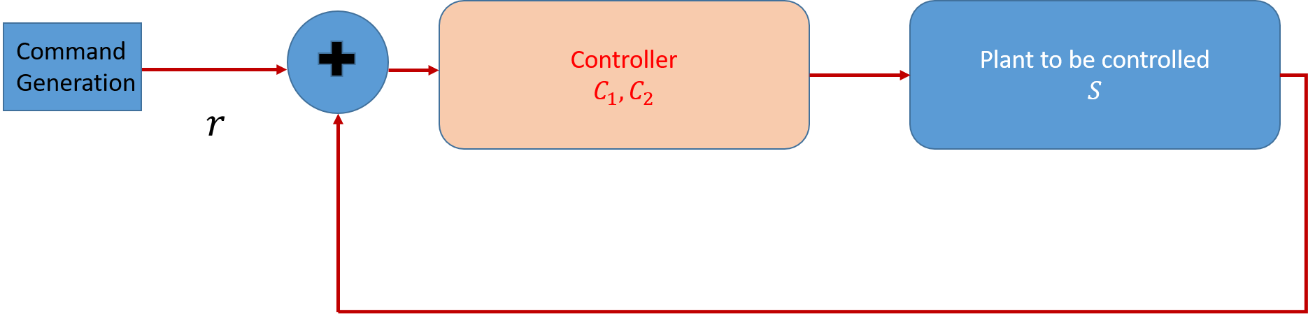
the dynamic system is described as in (4), (11), (120) for the linear case, or (3), or (90) in the nonlinear case. The adaptive controllers have a general form as in (6)-(7), which in linear systems are of the form (36) in simple cases, (40)-(42) when states are accessible, (50) and (54)-(55) or (63) for adaptive output feedback. For nonlinear problems, a few examples were outlined in (97)-(103). In most of the cases, it should be noted that the solutions provided are global, with the adaptive system starting from arbitrary initial conditions, and are applicable in real-time. No training, exploration or simulation experiments are required. These are unique features and advantages of the adaptive control method. The guarantees that the adaptive control solutions provide are predicated on assumptions that some prior information is available about the plant. Examples are information about its order, net-order, and the sign of the high frequency gain for the linear case. In a nonlinear plant, the assumptions pertain to a certain type of interconnection such as strict-feedback form (Krstić et al. 1995), triangular structures (Seto et al. 1994), or feedback linearization (Slotine and Li 1991). It should again be mentioned that in almost all of these cases, the underlying solutions are provably correct, with firm analytical guarantees and precise descriptions of the nature of the solutions.
Several efforts have been consistently and continuously applied over the years to relax these assumptions. An approach credited to Nussbaum (Nussbaum 1983) relaxes the requirement that the sign of the high frequency gain be known. The approach outlined in section 4.1.6 under high-order tuners only requires the net-order, but not the order, to be known. Several extensions to nonminimum phase systems have been reported over the years (Elliott et al. 1985). In some cases, these extensions come with other drawbacks such as lack of robustness due to an intrinsic high-gain nature, requirements of persistent excitation, or significant increase in the computational burden.
The importance of the interconnection between adaptation and learning cannot be over emphasized. The stability results outlined in Section 4.1 focused on just that, stability. No requirements on learning the unknown parameter were involved. Additional conditions of persistent excitation, if imposed, led to learning. In closed-loop, as one cannot guarantee that such PE conditions can be satisfied, one cannot guarantee learning. Rather, with imperfect learning, the adaptive control solutions guaranteed closed-loop boundedness and asymptotic guarantee of performance. If additional conditions are met, then learning follows. Optimality of the adaptive controller, when learning is complete, can subsequently be ensured. As was evident from the discussions in Section 4.6, robustness of these performance goals under various conditions and perturbations have also been guaranteed.
As we proceed to expand the scope of the class of dynamic systems under consideration, we articulate one of the main challenges that is encountered due to the interconnection and compelling tradeoffs between adaptation and learning. Suppose we address the closed-loop control in Figure 1, where is given by (3).
Suppose that the control input is generated using a neural network with its input as follows:
| (144) |
where denotes the number of layers, , , , denote the weights in the th layer, , and are respectively the input and output of the neural controller. denotes the activation function. Suppose that the neural network is trained extensively for a given set of parameters in the dynamic system so that the closed-loop system generates a performance that is satisfactory. It should be noted that the parameters of the neural network, converge (if they do; no analytical guarantees exist as of today that they converge) to some value such that the mapping between and approximate the desired nonlinear mapping. At this point, suppose that the plant parameter in changes in an unbeknownst manner that cannot be anticipated beforehand and accompanied by non-parametric changes in disturbances or unmodeled dynamics. The closed-loop system in such a case is highly prone to the bursting phenomenon described in Section IV-I, in the multi-dimensional space made up of weights, states, and inputs of the overall closed-loop system, as the system may not have been trained satisfactorily at these changed conditions. It is the analysis of this resulting closed-loop system together with guarantees of boundedness, convergence, and optimality that is needed. This is an open problem that needs to be addressed.
4.10 Loci of Adaptive Control
As mentioned in the introduction, the focus of this article is on those aspects of adaptive control that has an identifiable learning component with tractable problem formulations and solutions. It should be noted that huge swaths of efforts have been expended in several other branches of adaptive control over the past five decades with enormous success. We mention but a few of those classes that capture the loci of adaptive control.
Extensions to adaptive control of infinite dimensional systems can be found in (Smyshlyaev and Krstic 2010) and a special class of problems which corresponds to systems with delays (Ortega and Lozano 1988; Niculescu and Annaswamy 2003; Yildiz et al. 2010a; Bresch-Pietri and Krstic 2009; Bresch-Pietri and Krstic 2014). They have found applications in traffic control (Burkhardt et al. 2021), power-train control (Yildiz et al. 2010b), rocket pressure control (Alan et al. 2018), and drilling (Krstic 2013), to name a few. In most of these cases, these approaches consist of adaptive controller designs with an in-built parameter estimate, with requisite complexities in both the control and adaptive law as well as in the machineries employed. Additional tools from infinite dimensional systems and Lyapunov functions need to be utilized to derive stable solutions. The goals of these designs are to primarily accomplish the control goal; learning, i.e. convergence of the underlying estimates to the true value are very hard to establish.
Interesting extensions have been reported in (Guo 1997; Xie and Guo 2000; Huang and Guo 2012) for necessary and sufficient conditions for control of classes of systems under uncertainties, in an attempt to examine fundamental limitations of the feedback mechanism. A computationally tractable solution to the adaptive stabilization problem addressed in Huang and Guo 2012 is proposed in (Sokolov 2016a; Sokolov 2016b) based on set estimation with Yakubovich’s method of recursive goal inequalities. This and related directions are surveyed in (Guo 2020).
Several other branches of adaptive control have been investigated over the years. The first include decentralized and distributed adaptive control based on notions of cooperation and consensus, and adaptive control for synchronization of complex networks (Ioannou 1986; Lellis et al. 2009; Olgren et al. 2004; Zhou et al. 2006; Cao et al. 2008; Hou et al. 2009; Das and Lewis 2010). Another area is adaptive control in the presence of commonly present algebraic nonlinearities such as hysteresis (Tao and Kokotovic 1995) and deadzones (Tao and Kokotovic 1994), which are useful in all applications where actuator nonlinearities have to be contended with (Tao et al. 2004). Along with actuator nonlinearities, actuator redundancy has been addressed in (Tohidi et al. 2020) via adaptive control allocation methods. The use of a filter and high-gain in closed-loop (Hovakimyan and Cao 2010) has been explored as well with significant successes reported in applications. Yet another related topic that intersects with adaptive control and machine learning based optimization is extremum seeking. Here, the goal is to adjust a parameter, but not with the purpose of learning the parameter or an underlying function but to rather maximize a function (Krstić and Wang 2000; Ariyur and Krstic 2003). We expect interesting discoveries related to the intersections between these topics to unfold over the coming years.
The topics covered in this paper are by no means an exhaustive account of all control methods are adopted for dynamic systems with uncertain parameters. The most notable methods that we have not covered in this paper include adaptive sliding mode control (see for example, Bartolini et al. 1995; Huang et al. 2008; Lee et al. 2009), iterative learning control (see for example, Bristow et al. 2006,Moore 2012), and linear-parameter-varying systems (see for example, Mohammadpour and Scherer 2012; Hoffmann and Werner 2014). The reader is referred to the cited papers for a deeper dive into these methods.
5 Applications
Progress in theory has been accompanied throughout the past five decades with explorations of applications of adaptive control in various sectors. This is evidenced by edited books (Narendra 1980 (reprinted 2012), surveys (Åström 1983; Astrom 1996), chapters in textbooks (Landau et al. 2011; Narendra and Annaswamy 2005; Ulsoy and Koren 1989), or entire textbooks (Lavretsky and Wise 2013). Applications span process control (Dumont and Huzmezan 2002; Ismail et al. 2003; Dumont et al. 1990; Allison et al. 1995; Ismail et al. 2003), automotive systems (Yildiz et al. 2010b; Yildiz et al. 2010c), positioning systems (Ulsoy and Koren 1989; Smith et al. 1995), propulsion systems (Evesque et al. 2003b; Riley et al. 2004), and a huge effort in flight control (see for example, (Thompson and Welsh 1970),(Taylor et al. 1964; Dydek et al. 2010; Calise and Rysdyk 1998; Jenkins 2000; Boskovic et al. 2004),(Gregory et al. 2011),(Achtelik et al. 2011),(Dydek et al. 2012; Dydek et al. 2013b; Dydek et al. 2013a)).
Since the early 1990’s, the US Air Force, US Navy, and NASA working with industry and academia have made significant progress towards maturing adaptive control theory for aerospace applications (Gregory et al. 2011). Several adaptive control architectures have been implemented in unmanned flight platforms (Sharma et al. 2006). A specific observer-based adaptive control with Loop Transfer Recovery (OBLTR) has been developed in Lavretsky and Wise 2013. As pointed out in (Wise 2018), a technology transition of conventional MRAC applications and adaptive OBLTR based architectures, has been continuously ongoing (see Figure 1, Figure 4 in (Wise 2018)) which includes aerial platforms such as JDAM, X-36, and several others.
The reader is referred to the surveys and textbooks mentioned above for several more applications in addition to all of the above, for autopilots for ships, and coworkers, cement mills, chemical reactors, diesel engines, glass furnaces, heating and ventilation, motor drives, paper machines, optical telescopes and titanium oxide kilns, and more. The reader is referred to Samad and Annaswamy 2011 for additional success stories.
Several industrial products exist that implement MRAC and STR described above. NOVATUNE and NOVAMAX produced by ASEA AB were early examples mentioned in the 80s in Åström 1983. The reference Dumont and Huzmezan 2002 lists BrainWave, an adaptive MPC, and MicroController 2000X, both implemented in several process control problems. We also refer the reader to the proceedings of several workshops in conferences such as the ACC, CCTA, and CDC, that have presented recent applications of adaptive control to aerospace problems (see for example (Hull and Cichella 2021)).
In much of these applications, the need for adaptive control stems from a scenario where a control problem arises and a satisfactory solution requires a retuning of the control parameters due to aging, drift, or other untoward changes in the plant being controlled. The existing baseline controller becomes, as a result, incorrect, and needs to be retuned. In several of these applications, such as in autonomous vehicles either in air, ground, or water, may require this self-tuning or adaptation, to occur on the fly, in real time. The flight platforms considered in (Sharma et al. 2006) and other flight platforms listed above fall under this category. Often the existing baseline controllers become inadequate under these anomalies, may be destabilizing, and need to be retuned. And under these circumstances, adaptive control enables a procedure by which real-time adjustment of controllers is possible. That adaptive controllers are finding a pathway for technology transition, systematic validation, and field implementation is clear from the above discussions. The relatively slower pace of implementation of adaptive technologies, compared to say MPC, may be a combination of the need for a truly real-time tuning in a given application and the requisite bandwidth and complexity for implementation. As applications become more complex and as computing and communication technologies become more advanced, both of this impediments may very likely diminish and disappear.
6 Summary and Concluding Remarks
In this paper, we have sketched a historical perspective of the field of adaptive control over the past seven decades. Given the recent upsurge of interest in learning, both offline and online, in the Machine Learning and control communities, such a perspective is timely and warranted. The scope of this article is large - we have attempted to cover highlights of the field which span 70 years, chronicled in 15 textbooks, 20 edited books, hundreds of surveys, and thousands of research publications in journals and conferences in 30 pages, which is a formidable task. We have therefore showcased just the highlights of this field, and emphasized key lessons learned, problems that have already been solved, important takeaway messages, and cautionary remarks. While our attempts at chronology span the footprint of this topic from the 1950s to the present, it should be acknowledged that there is a large vigorous set of activities in this area over the last five to ten years, especially at the intersection of parameter learning, reinforcement learning, neural networks, and adaptive control that we have not addressed in this paper. We refer the reader to recent plenary talks, papers in recent control and machine learning conferences, and special issues in related journals for the exposition of the latest advances.
Over the last seventy years, the field of adaptive control has witnessed advances in both deterministic and continuous-time systems and stochastic discrete-time systems. We have attempted to cover both domains in this article. Key advances in different parts of the globe have all been attempted to be covered. We have not offered a deep technical discussion of theorems, but rather the idea behind key results and their implications. No proofs have been provided either. The reader is referred to the list of copious references at the end of the paper for in-depth technical expositions of all problems and solutions outlined here. We presented a chronological taxonomy of the advances in the field in Section II, a cross-section of problem statements in Section III, and highlights of key solutions in Section IV. Major applications of adaptive control are addressed in Section V.
The primary focus of the adaptive controllers has been to ensure that (a) the closed-loop system have bounded solutions, and (b) asymptotic properties of the outputs (and in some cases inputs) are achieved. The results in 4.8 have extended this focus and have made inroads in making sure that the requisite constraints of magnitude and rate for the control input and state constraints are met as well. It should be noted that in all cases, the performance goals have been limited to the system behavior in real-time, at time , and not for all future instants. As the premise in all these problems is that parametric uncertainties can be introduced at any time, optimization of a cost function over all time, with a cold-start of the controller that simultaneously estimates, adapts, and optimizes, is difficult if not impossible. Some of the recent results that propose clever combinations of both adaptive control and machine learning concepts may overcome this formidable challenge.
Acknowledgements
We would like to thank P.R. Kumar for several useful discussions and directing us to the highlights of stochastic adaptive control. We would like thank the reviewers and Miroslav Krstic for their valuable comments which helped place our overall message in the broader and rich landscape of adaptive control theory. We would like to gratefully acknowledge Yingnan Cui and Boris Andrievsky for helping us build the database with almost 300 references on adaptive control and learning.
Appendix
Stability framework
The first and foremost challenge introduced by adaptive control is a nonlinearity. As the controller is proposed as a real-time control solution, the nonlinearity is introduced due to the simultaneous estimation and control. That is, the control input is a function of the parameter estimate which in turn depends on the control input as well as several other system variables. As a result, the closed-loop system becomes nonlinear, with its solutions corresponding to the true responses of the plant being controlled. As a result, the well behavedness of the overall adaptive system, i.e. its stability is the first property that needs to be assured. The typical tool employed here is due to Lyapunov and is summarized below Narendra and Annaswamy 2005. The dynamic system of interest is of the form
| (145) |
It is assumed that is such that a solution exists for all .
Theorem 3
The equilibrium state of (145) is uniformly asymptotically stable in the large if a scalar function with continuous first partial derivatives w.r.t and exists such that and if the following conditions are satisfied:
- (i)
is positive-definite,
- (ii)
is decrescent,
- (iii)
is negative-definite, and
- (iv)
is radially unbounded.
that satisfies these conditions is referred to as a Lyapunov function. If instead of (iii), is only negative semi-definite, only uniform stability can be ensured; if instead of (iii), a stronger condition , then exponential stability of the equilibrium can be ensured. We refer the reader to Narendra and Annaswamy 2005 for all further technical details.
A typical approach in adaptive control is to express the underlying system in the form of (145) with the state corresponding to errors in the system that are either to be driven to zero or required to be bounded. These error can be broadly grouped into two categories, tracking error and parameter error. Often adaptive systems consider quadratic Lyapunov function and only lead to a negative semi-definite .
Rational SPR functions and the KYL
The definition of SPR and one of the simplest versions of the KYL Anderson and Johnson 1982 is given below.
Definition: An matrix , whose elements are rational transfer function, is SPR if for some and all ,
- 1.
all elements of are analytic
- 2.
, and
- 3.
is positive semi-definite.
The Kalman Yakubovich Lemma
Let be a matrix of rational functions with , a minimal realization , and with all its poles only in . Then is SPR if and only if there exist symmetric positive definite matrices such that
| (146) |
Bregman Divergence
Further extensions can be obtained based on the Bregman divergence construction Boffi and Slotine 2021. Let be a twice differentiable function, . Let , where is the gradient of the function . The function turns out to be convenient to use for the convergence proofs as a part of extended Lyapunov function. For example, extended versions of the speed-gradient algorithm can be designed via a Lyapunov function Boffi and Slotine 2021
| (147) |
It leads to the algorithms
| (148) |
generalizing algorithms (88).
Averaging
A standard method that has been studied extensively in the area of nonlinear oscillations has been utilized often in adaptive systems in the context of robustness with respect to disturbances and unmodeled dynamics Anderson et al. 1986. This is briefly summarized below. Originally suggested in Krylov and Bogoliubov 1937 (Translated by Princeton University Press, Princeton, 1947 and expanded in Bogoliubov and Mitropolskij 1961; Sanders and Verhulst 1985, this method is associated with the solutions of a differential equation
| (149) |
where is a positive constant. An approximate solution for (149) can be found if is small and the solution varies slowly using the process of averaging. The underlying idea here is that as is varying slowly, the rapidly varying terms in do not affect the slow variation of in the long run. We briefly outline the application of this tool to adaptive systems Anderson et al. 1986; Kokotovic et al. 1985: The underlying error model for the perturbed system in (8), when only unmodeled dynamics are present and the adaptive law as in (54) and (55) is used can be written as
| (150) |
where corresponds to the realization of the closed-loop transfer function that arises when there is no parametric uncertainty, and denotes the system variables that are accessible. That is, . The robustness of the adaptive system is assured if the solutions of (150) are well behaved. The following theorem outlines this result Kokotovic et al. 1985: Let be bounded, almost periodic, and persistently exciting. Then
- 1.
there exists a such that for all , the origin of (150) is exponentially stable if
(151) - 2.
The condition (151) is satisfied if
(152)
An expansion of using an inverse Fourier transform expansion such as is leveraged in this context. Eq. (152) implies that the stability property of (150) critically depends on the spectrum of the excitation of in relation to the closed-loop transfer function . More importantly, the condition in (151) can be met by a large class of problems where is not SPR.
References
- Abramson et al. (1963) Abramson, N., Braverman, D., Sebestyen, G., 1963. Pattern recognition and machine learning. IEEE Transactions on Information Theory 9.
- Achtelik et al. (2011) Achtelik, M., Bierling, T., Wang, J., Höcht, L., Holzapfel, F., 2011. Adaptive control of a quadcopter in the presence of large/complete parameter uncertainties, in: Infotech@ Aerospace 2011, p. 1485.
- Aizerman (1963) Aizerman, M., 1963. The problem of training an automaton to perform classification of input situations (pattern recognition). Theory Self-Adapt. Contr. Syst. Proc. IFAC Symp. 2nd .
- Alan et al. (2018) Alan, A., Yildiz, Y., Poyraz, U., 2018. High-performance adaptive pressure control in the presence of time delays: Pressure control for use in variable-thrust rocket development. IEEE Control Systems Magazine 38, 26–52.
- Allison et al. (1995) Allison, B.J., Ciarniello, J.E., Tessier, P.J.C., Dumont, G.A., 1995. Dual adaptive control of chip refiner motor load. Automatica 31, 1169–1184.
- Ames et al. (2014) Ames, A.D., Grizzle, J.W., Tabuada, P., 2014. Control barrier function based quadratic programs with application to adaptive cruise control, in: 53rd IEEE Conference on Decision and Control, IEEE. pp. 6271–6278.
- Anderson et al. (1986) Anderson, B., Bitmead, R.R., Johnson Jr, C.R., Kokotovic, P.V., Kosut, R.L., Mareels, I.M., Praly, L., Riedle, B.D., 1986. Stability of Adaptive Systems: Passivity and Averaging Analysis. MIT press.
- Anderson and Johnson (1982) Anderson, B.D., Johnson, C., 1982. Exponential convergence of adaptive identification and control algorithms. Automatica 18, 1–13. doi:10.1016/0005-1098(82)90021-8.
- Anderson (1985) Anderson, B.D.O., 1985. Adaptive systems, lack of persistency of excitation and bursting phenomena. Automatica 21, 247–258.
- Andrievskii and Fradkov (2006) Andrievskii, B., Fradkov, A., 2006. Method of passification in adaptive control, estimation, and synchronization. Autom. Remote Control 67, 1699––1731.
- Andrievskii and Selivanov (2018) Andrievskii, B., Selivanov, A., 2018. New results on the application of the passification method. a survey. Autom. Remote Control 79, 957–995.
- Andrievsky and Fradkov (2021) Andrievsky, B.R., Fradkov, A.L., 2021. Method of speed-gradient and its applications. Automation and Remote Control 9, 5–78.
- Andrievsky B. (2020) Andrievsky B., S.A., 2020. Historical overview of the passification method and its applications to nonlinear and adaptive control problems. European Control Conference 19, 791–794.
- Annaswamy and Karason (1995) Annaswamy, A.M., Karason, S., 1995. Discrete-time adaptive control in the presence of input constraints. Automatica 31, 1421–1431.
- Annaswamy et al. (1998a) Annaswamy, A.M., Skantze, F.P., Loh, A.P., 1998a. Adaptive control of continuous time systems with convex/concave parametrization. Automatica 34, 33–49.
- Annaswamy et al. (1998b) Annaswamy, A.M., Thanomsat, C., Mehta, N., Loh, A.P., 1998b. Applications of adaptive controllers to systems with nonlinear parametrization. ASME Journal of Dynamic Systems, Measurement, and Control .
- Aranovskiy et al. (2019) Aranovskiy, S., Belov, A., Ortega, R., Barabanov, N., Bobtsov, A., 2019. Parameter identification of linear time-invariant systems using dynamic regressor extension and mixing. International Journal of Adaptive Control and Signal Processing 33, 1016–1030.
- Ariyur and Krstic (2003) Ariyur, K.B., Krstic, M., 2003. Real-time optimization by extremum-seeking control. John Wiley & Sons.
- Aseltine et al. (1958) Aseltine, J., Mancini, A., Sarture, C., 1958. A survey of adaptive control systems. IRE Transactions on Automatic Control 6, 102–108.
- Asher et al. (1976) Asher, R.B., Andrisani, D., Dorato, P., 1976. Bibliography on adaptive control systems. Proceedings of the IEEE 64, 1226–1240.
- Astolfi et al. (2007) Astolfi, A., Karagiannis, D., Ortega, R., 2007. Nonlinear and adaptive control with applications. Springer Science & Business Media.
- Astolfi and Ortega (2003) Astolfi, A., Ortega, R., 2003. Immersion and invariance: A new tool for stabilization and adaptive control of nonlinear systems. IEEE Transactions on Automatic Control 48, 590–606.
- Astrom and Wittenmark (1973) Astrom, K., Wittenmark, B., 1973. On self tuning regulators. Automatica 9, 185–199.
- Åström (1983) Åström, K.J., 1983. Theory and applications of adaptive control—a survey. Automatica 19, 471–486.
- Astrom (1996) Astrom, K.J., 1996. Adaptive control around 1960. IEEE Control Systems Magazine 16, 44–49.
- Åström (2012) Åström, K.J., 2012. Introduction to stochastic control theory. Courier Corporation.
- Åström and Wittenmark (1995) Åström, K.J., Wittenmark, B., 1995. Adaptive Control: Second Edition. Addison-Wesley Publishing Company.
- A.Y.Chervonenkis (2013) A.Y.Chervonenkis, 2013. Early history of support vector machines., in: Empirical Inference: Festschrift in Honor of Vladimir N. Vapnik, Springer-Verlag Berlin Heidelberg. pp. 13–20.
- Bartolini et al. (1995) Bartolini, G., Ferrara, A., Utkin, V.I., 1995. Adaptive sliding mode control in discrete-time systems. Automatica 31, 769–773.
- Becker et al. (1985) Becker, A., Kumar, P.R., Wei, C.Z., 1985. Adaptive control with the stochastic approximation algorithm: Geometry and convergence. IEEE Transactions on Automatic Control 30, 330–338.
- Bellman (2015) Bellman, R.E., 2015. Adaptive control processes. Princeton university press.
- Bellman and Kalaba (1959) Bellman, R.E., Kalaba, R., 1959. On adaptive control processes. IRE Transactions on Automatic Control 4, 1–9.
- Bertsekas (2017) Bertsekas, D., 2017. Value and policy iterations in optimal control and adaptive dynamic programming. IEEE Trans. Neural Netw. Learn. Syst. 28, 500–509.
- Bertsekas (2008) Bertsekas, D.P., 2008. Approximate dynamic programming. Citeseer.
- Bian and Jiang (2016) Bian, T., Jiang, Z.P., 2016. Value iteration, adaptive dynamic programming, and optimal control of nonlinear systems. Proc. IEEE 55th Conf. Decis. Control (CDC). , 3375–3380.
- Bian and Jiang (2021) Bian, T., Jiang, Z.P., 2021. Reinforcement learning and adaptive optimal control for continuous-time nonlinear systems: A value iteration approach. IEEE Trans. Neural Netw. Learn. Syst. .
- Bitmead (1983) Bitmead, R., 1983. Convergence in distribution of lms-type adaptive parameter estimates. IEEE Transactions on Automatic Control 28, 54–60.
- Boffi and Slotine (2021) Boffi, N.M., Slotine, J.J.E., 2021. Implicit regularization and momentum algorithms in nonlinearly parameterized adaptive control and prediction. Neural Computation 33, 590–673.
- Bogoliubov and Mitropolskij (1961) Bogoliubov, N.N., Mitropolskij, Y., 1961. Asymptotic methods in the theory of nonlinear oscillations. Gordon and Breach, 1st edition.
- Bondarko and Yakubovich (1992) Bondarko, V., Yakubovich, V., 1992. The method of recursive aim inequalities in adaptive control theory. International Journal of Adaptive Control and Signal Processing. 6, 141–160.
- Bongard (1961) Bongard, M., 1961. Simulation of the recognition process on a digital computing machine. Biophysics 4.
- Borkar and Varaiya (1979) Borkar, V., Varaiya, P., 1979. Adaptive control of markov chains, i: Finite parameter set. IEEE Transactions on Automatic Control 24, 953–957.
- Boskovic et al. (2004) Boskovic, J.D., Chen, L., Mehra, R.K., 2004. Adaptive control design for nonaffine models arising in flight control. Journal of guidance, control, and dynamics 27, 209–217.
- Boyd and Sastry (1983) Boyd, S., Sastry, S., 1983. On parameter convergence in adaptive control. Systems & Control Letters 3, 311–319. doi:10.1016/0167-6911(83)90071-3.
- Braverman (1962) Braverman, E., 1962. The experiments with training a machine to recognize patterns. Automat. Remote Contr. 23.
- Bregman (1967) Bregman, L., 1967. The relaxation method of finding the common point of convex sets and its application to the solution of problems in convex programming. USSR Computational Mathematics and Mathematical Physics 7, 200–217.
- Bresch-Pietri and Krstic (2009) Bresch-Pietri, D., Krstic, M., 2009. Adaptive trajectory tracking despite unknown input delay and plant parameters. Automatica 45, 2074–2081.
- Bresch-Pietri and Krstic (2014) Bresch-Pietri, D., Krstic, M., 2014. Delay-adaptive control for nonlinear systems. IEEE Transactions on Automatic Control 59, 1203–1218.
- Bristow et al. (2006) Bristow, D.A., Tharayil, M., Alleyne, A.G., 2006. A survey of iterative learning control. IEEE control systems magazine 26, 96–114.
- Burkhardt et al. (2021) Burkhardt, M., Yu, H., Krstic, M., 2021. Stop-and-go suppression in two-class congested traffic. Autom. 125, 109381. URL: https://doi.org/10.1016/j.automatica.2020.109381, doi:10.1016/j.automatica.2020.109381.
- Caines (1992) Caines, P., 1992. Continuous time stochastic adaptive control: non-explosion, eps-consistency and stability. Systems and Control Letters 19, 169–176.
- Caines and Lafortune (1984) Caines, P., Lafortune, S., 1984. Adaptive control with recursive identification for stochastic linear systems. IEEE Transactions on Automatic Control 29, 312–321.
- Caldwell (1950) Caldwell, W.I., 1950. Control system with automatic response adjustment. US Patent 2,517,081.
- Calise and Rysdyk (1998) Calise, A.J., Rysdyk, R.T., 1998. Nonlinear adaptive flight control using neural networks. IEEE Control Systems Magazine 18, 14–25.
- Campi and Kumar (1996) Campi, M.C., Kumar, P.R., 1996. Optimal adaptive control of an lqg system, in: Proceedings of 35th IEEE Conference on Decision and Control, IEEE. pp. 349–353.
- Campi and Kumar (1998) Campi, M.C., Kumar, P.R., 1998. Adaptive linear quadratic gaussian control: the cost-biased approach revisited. SIAM Journal on Control and Optimization 36, 1890–1907.
- Cao et al. (2003) Cao, C., Annaswamy, A.M., Kojic, A., 2003. Parameter convergence in nonlinearly parameterized systems. IEEE Transactions on Automatic Control 48, 397–412. doi:10.1109/TAC.2003.809146.
- Cao et al. (2008) Cao, M., Morse, A.S., Anderson, B.D.O., 2008. Reaching a consensus in a dynamically changing environment: convergence rates, measurement delays, and asynchronous events. SIAM Journal on Control and Optimization 47, 601–623.
- Chang et al. (2013) Chang, H.S., Fu, M.C., Hu, J., Marcus, S.I., 2013. Simulation-Based Algorithms for Markov Decision Processes. Springer Science & Business Media.
- Chang et al. (2019) Chang, Y.C., Roohi, N., Gao, S., 2019. Neural lyapunov control. Advances in Neural Information Processing Systems 32, 3245–3254.
- Chaoui et al. (2001) Chaoui, F., Giri, F., M’Saad, M., 2001. Adaptive control of input-constrained type-1 plants stabilization and tracking. Automatica 37, 197–203.
- Chen and Chen (1984) Chen, C.T., Chen, C.T., 1984. Linear system theory and design. volume 301. Holt, Rinehart and Winston New York.
- Clarke et al. (1985) Clarke, D., Kanjilal, P., Mohtadi, C., 1985. A generalized lqg approach to self-tuning control part i. aspects of design. International Journal of Control 41, 1509–1523.
- Clarke and Gawthrop (1979) Clarke, D.W., Gawthrop, P.J., 1979. Self-tuning control, in: Proceedings of the Institution of Electrical Engineers, IET. pp. 633–640.
- Cluett et al. (1988) Cluett, W., Shah, S., Fisher, D., 1988. Robustness analysis of discrete-time adaptive control systems using input-output stability theory: A tutorial, in: IEEE Proceedings D-Control Theory and Applications, IET. pp. 133–141.
- Das and Lewis (2010) Das, A., Lewis, F.L., 2010. Distributed adaptive control for synchronization of unknown nonlinear networked systems. Automatica 46, 2014–2021.
- Dogan et al. (2016) Dogan, K.M., Yucelen, T., Gruenwald, B.C., Muse, J.A., 2016. On model reference adaptive control for uncertain dynamical systems with unmodeled dynamics, in: 2016 IEEE 55th Conference on Decision and Control (CDC), IEEE. pp. 377–382.
- Drenick and Shahbender (1957) Drenick, R., Shahbender, R., 1957. Adaptive servomechanisms. Transactions of the American Institute of Electrical Engineers, Part II: Applications and Industry 76, 286–292.
- Duarte and Narendra (1989) Duarte, M.A., Narendra, K.S., 1989. Combined direct and indirect approach to adaptive control. IEEE Transactions on Automatic Control 34, 1071–1075.
- Dumont and Huzmezan (2002) Dumont, G.A., Huzmezan, M., 2002. Concepts, methods and techniques in adaptive control, in: Proceedings of the 2002 American control conference (IEEE Cat. No. CH37301), IEEE. pp. 1137–1150.
- Dumont et al. (1990) Dumont, G.A., Zervos, C.C., Pageau, G.L., 1990. Laguerre-based adaptive control of ph in an industrial bleach plant extraction stage. Automatica 26, 781–787.
- Duncan et al. (1999) Duncan, T., Guo, L., Pasik-Duncan, B., 1999. Adaptive continuous-time linear quadratic gaussian control. IEEE Transactions on Automatic Control 44, 1653–1662.
- Duncan and Pasik-Duncan (1990) Duncan, T.E., Pasik-Duncan, B., 1990. Adaptive control of continuous-time linear stochastic systems. Mathematics of Control, signals and systems 3, 45–60.
- Dydek et al. (2010) Dydek, Z.T., Annaswamy, A.M., Lavretsky, E., 2010. Adaptive control and the NASA X-15-3 flight revisited. IEEE Control Systems Magazine 30, 32–48.
- Dydek et al. (2012) Dydek, Z.T., Annaswamy, A.M., Lavretsky, E., 2012. Adaptive control of quadrotor UAVs: a design trade study with flight evaluations. IEEE Transactions on control systems technology 21, 1400–1406.
- Dydek et al. (2013a) Dydek, Z.T., Annaswamy, A.M., Lavretsky, E., 2013a. Adaptive configuration control of multiple uavs. Control Engineering Practice 21, 1043–1052.
- Dydek et al. (2013b) Dydek, Z.T., Annaswamy, A.M., Slotine, J.J.E., Lavretsky, E., 2013b. Composite adaptive posicast control for a class of LTI plants with known delay. Automatica 49, 1914–1924.
- Egardt (1979) Egardt, B., 1979. Stability of adaptive controllers. volume 20. Springer.
- Elliott et al. (1985) Elliott, H., Cristi, R., Das, M., 1985. Global stability of adaptive pole placement algorithms. IEEE transactions on automatic control 30, 348–356.
- Evesque et al. (2003a) Evesque, S., Annaswamy, A.M., Niculescu, S., Dowling, A.P., 2003a. Adaptive control of a class of time-delay systems. J. Dyn. Sys., Meas., Control 125, 186–193.
- Evesque et al. (2003b) Evesque, S., Dowling, A.P., Annaswamy, A.M., 2003b. Self-tuning regulators for combustion oscillations. Proceedings of the Royal Society of London. Series A: Mathematical, Physical and Engineering Sciences 459, 1709–1749.
- Feldbaum (1960a) Feldbaum, A., 1960a. Dual control theory. i. Avtomatika i Telemekhanika 21, 1240–1249.
- Feldbaum (1960b) Feldbaum, A., 1960b. Dual control theory. parts i, ii. Automation and Remote Control 21.
- Fomin (1991) Fomin, V., 1991. Chapter 6. adaptive control of stochastic systems, in: Discrete Linear Control Systems. Kluwer, Dordrecht/Boston/London, pp. 221–284.
- Fomin et al. (1981) Fomin, V., Fradkov, A.L., Yakubovich, V., 1981. Adaptive control of dynamical systems. Nauka, Moskow.
- Fortescue et al. (1981) Fortescue, T., Kershenbaum, L.S., Ydstie, B.E., 1981. Implementation of self-tuning regulators with variable forgetting factors. Automatica 17, 831–835.
- Fradkov (1974) Fradkov, A., 1974. Synthesis of adaptive system of stabilization for linear dynamic plants. Autom. Remote Control , 1960–1966.
- Fradkov (2003) Fradkov, A., 2003. Passification of nonsquare linear systems and feedback yakubovich-kalman-popov lemma. Europ. J. Control , 573–582.
- Fradkov and Lipkovich (2015) Fradkov, A., Lipkovich, M., 2015. Adaptive absolute stability. IFAC-PapersOnLine 48, 258–263.
- Fradkov et al. (1999) Fradkov, A., Miroshnik, I., Nikiforov, V., 1999. Nonlinear and Adaptive Control of Complex Systems. volume 491. Kluwer Academic Publications.
- Fradkov (1980) Fradkov, A.L., 1980. Speed-gradient scheme and its application in adaptive control problems. Autom. Remote Control 40, 1333–1342. (Translated from Avtomat. i Telemekh., 1979, issue 9, 90–101).
- Fradkov (1987) Fradkov, A.L., 1987. Synthesizing adaptive-control systems for nonlinear singularly perturbed objects. Autom. Remote Control 48, 789–798.
- Fradkov (2020) Fradkov, A.L., 2020. Early history of machine learning. IFAC-PapersOnLine 53, 1385–1390.
- Fradkov et al. (2001) Fradkov, A.L., Ortega, R., Bastin, G., 2001. Semi-adaptive control of convexly parametrized systems with application to temperature regulation of chemical reactors. International Journal of Adaptive Control and Signal Processing 15, 415–426.
- Fradkov and Polyak (2020) Fradkov, A.L., Polyak, B., 2020. Adaptive and robust control in the ussr. IFAC-PapersOnLine 53, 1373–1378.
- Gaudio et al. (2018) Gaudio, J.E., Annaswamy, A.M., Lavretsky, E., 2018. Adaptive control of hypersonic vehicles in the presence of rate limits, in: 2018 AIAA Guidance, Navigation, and Control Conference, p. 0846.
- Gaudio et al. (2020a) Gaudio, J.E., Annaswamy, A.M., Lavretsky, E., Bolender, M.A., 2020a. Fast parameter convergence in adaptive flight control. 2020 AIAA Guidance, Navigation, and Control Conference .
- Gaudio et al. (2020b) Gaudio, J.E., Annaswamy, A.M., Moreu, J.M., Bolender, M.A., Gibson, T.E., 2020b. Accelerated learning with robustness to adversarial regressors. Proceedings of the 3rd Conference on Learning for Dynamics and Control, PMLR 144:636-650 .
- Gevers et al. (1991) Gevers, M., G.C., G., Wertz, V., 1991. Continuous-time stochastic adaptive control. SIAM Journal on Control and Optimization 29, 264–282.
- Gittins (1979) Gittins, J.C., 1979. Bandit processes and dynamic allocation indices. Journal of the Royal Statistical Society: Series B (Methodological) 41, 148–164.
- Goodwin et al. (1980) Goodwin, G.C., Ramadge, P.J., Caines, P.E., 1980. Discrete-time multivariable adaptive control. IEEE Transactions on Automatic Control 25, 449–456. doi:10.1109/TAC.1980.1102363.
- Goodwin et al. (1981) Goodwin, G.C., Ramadge, P.J., Caines, P.E., 1981. Discrete time stochastic adaptive control. SIAM Journal on Control and Optimization 19, 829–853. doi:10.1137/0319052.
- Grayson (1963) Grayson, L.P., 1963. Design via lyapunov’s second method, in: Joint Automatic Control Conference, pp. 589–595.
- Gregory et al. (2011) Gregory, I., Gadient, R., Lavretsky, E., 2011. Flight test of composite model reference adaptive control (cmrac) augmentation using nasa airstar infrastructure, in: AIAA guidance, navigation, and control conference, p. 6452.
- Gregory (1959) Gregory, P., 1959. Proceedings of the Self-adaptive Flight Control Systems Symposium. Technical Report. Aeronautical Systems Div Wright-Patterson AFB OH Flight Control Lab.
- Gubin et al. (1967) Gubin, L., Polyak, B., Raik, E., 1967. The method of projections for finding the common point of convex sets. USSR Computational Mathematics and Mathematical Physics 7, 1–24.
- Guo (1995) Guo, L., 1995. Convergence and logarithm laws of self-tuning regulators. Automatica 31, 435–450.
- Guo (1997) Guo, L., 1997. On critical stability of discrete-time adaptive nonlinear control. IEEE Transactions on Automatic Control 42, 1488–1499.
- Guo (2020) Guo, L., 2020. Feedback and uncertainty: Some basic problems and results. Annual Reviews in Control 49, 27–36.
- Guo and Chen (1991) Guo, L., Chen, H.F., 1991. The astrom-wittenmark self-tuning regulator revisited and els-based adaptive trackers. IEEE Transactions on Automatic Control 36, 802–812.
- Gusev (1988) Gusev, S., 1988. Linear stabilization of nonlinear systems program motion. Systems & control letters 11, 409–412.
- Haddad et al. (2001) Haddad, W.M., Chellaboina, V., Hayakawa, T., 2001. Robust adaptive control for nonlinear uncertain systems. Proc. 40th IEEE Conference on Decision and Control 2, 1615–1620.
- Hammond (2013) Hammond, P.H., 2013. Theory of Self-Adaptive Control Systems: Proceedings of the Second IFAC Symposium on the Theory of Self-Adaptive Control Systems September 14–17, 1965 National Physical Laboratory Teddington, England. Springer.
- Harris (1981) Harris, C.J., 1981. Self-tuning and adaptive control: theory and applications. Peter Peregrinus.
- Hebb (1949) Hebb, D.O., 1949. The organisation of behaviour: a neuropsychological theory. Science Editions New York.
- Hoffmann and Werner (2014) Hoffmann, C., Werner, H., 2014. A survey of linear parameter-varying control applications validated by experiments or high-fidelity simulations. IEEE Transactions on Control Systems Technology 23, 416–433.
- Hou et al. (2009) Hou, Z.G., Cheng, L., Tan, M., 2009. Decentralized robust adaptive control for the multiagent system consensus problem using neural networks. IEEE Transactions on Systems, Man, and Cybernetics, Part B (Cybernetics) 39, 636–647.
- Hovakimyan and Cao (2010) Hovakimyan, N., Cao, C., 2010. L1 adaptive control theory: Guaranteed robustness with fast adaptation. SIAM.
- Huang and Guo (2012) Huang, C., Guo, L., 2012. On feedback capability for a class of semiparametric uncertain systems. Automatica 48, 873–878.
- Huang et al. (2008) Huang, Y.J., Kuo, T.C., Chang, S.H., 2008. Adaptive sliding-mode control for nonlinearsystems with uncertain parameters. IEEE Transactions on Systems, Man, and Cybernetics, Part B (Cybernetics) 38, 534–539.
- Hull and Cichella (2021) Hull, R., Cichella, V., 2021. Workshop on multi-vehicle and assured autonomous control for aerospace applications. Conference on Control Technology and Applications .
- Hussain (2017) Hussain, H.S., 2017. Robust Adaptive Control in the Presence of Unmodeled Dynamics. Ph.D. thesis. MIT.
- Hussain et al. (2013) Hussain, H.S., Matsutani, M., Annaswamy, A.M., Lavretsky, E., 2013. Robust adaptive control in the presence of unmodeled dynamics: A counter to Rohrs’s counterexample, in: AIAA Guidance, Navigation, and Control (GNC) Conference, p. 4753.
- Hussain et al. (2017) Hussain, H.S., Yildiz, Y., Matsutani, M., Annaswamy, A.M., Lavretsky, E., 2017. Computable delay margins for adaptive systems with state variables accessible. IEEE Transactions on Automatic Control 62, 5039–5054.
- Ioannou (1986) Ioannou, P., 1986. Decentralized adaptive control of interconnected systems. IEEE Transactions on Automatic Control 31, 291–298.
- Ioannou and Kokotovic (1984) Ioannou, P.A., Kokotovic, P.V., 1984. Instability analysis and improvement of robustness of adaptive control. Automatica 20, 583–594.
- Ioannou and Sun (1996) Ioannou, P.A., Sun, J., 1996. Robust Adaptive Control. PTR Prentice-Hall.
- Ioannou and Tsakalis (1986a) Ioannou, P.A., Tsakalis, K., 1986a. A robust direct adaptive controller. IEEE Transactions on Automatic control 31, 1033–1043.
- Ioannou and Tsakalis (1986b) Ioannou, P.A., Tsakalis, K., 1986b. Robust discrete-time adaptive control, in: Adaptive and Learning Systems. Springer, pp. 73–85.
- Ishii et al. (2002) Ishii, S., Yoshida, W., Yoshimoto, J., 2002. Control of exploitation–exploration meta-parameter in reinforcement learning. Neural networks 15, 665–687.
- Ismail et al. (2003) Ismail, A., Dumont, G.A., Backstrom, J., 2003. Dual adaptive control of paper coating. IEEE transactions on control systems technology 11, 289–309.
- Jenkins et al. (2019) Jenkins, B., Krupadanam, A., Annaswamy, A.M., 2019. Fast adaptive observers for battery management systems. IEEE Transactions on Control Systems Technology , 1–14.
- Jenkins et al. (2018) Jenkins, B.M., Annaswamy, A.M., Lavretsky, E., Gibson, T.E., 2018. Convergence properties of adaptive systems and the definition of exponential stability. SIAM journal on control and optimization 56, 2463–2484.
- Jenkins (2000) Jenkins, D.R., 2000. Hypersonics before the shuttle: A concise history of the X-15 research airplane. National Aeronautics and Space Admin., NASA Office of Policy and Plans, NASA ….
- Johansson (1995) Johansson, R., 1995. Supermartingale analysis of minimum variance adaptive control. Control-Theory and Advanced Technology (C-TAT) 10, 993–1013.
- Kaelbling et al. (1996) Kaelbling, L.P., Littman, M.L., Moore, A.W., 1996. Reinforcement learning: A survey. Journal of artificial intelligence research 4, 237–285.
- Kailath (1980) Kailath, T., 1980. Linear systems. volume 156. Prentice-Hall Englewood Cliffs, NJ.
- Kalman (1963) Kalman, R.E., 1963. Lyapunov functions for the problem of lur’e in automatic control. Proceedings of the National Academy of Sciences of the United States of America 49, 201.
- Karason and Annaswamy (1994) Karason, S.P., Annaswamy, A.M., 1994. Adaptive control in the presence of input constraints. IEEE Transactions on Automatic Control 39, 2325–2330. doi:10.1109/9.333787.
- Kokotovic et al. (1985) Kokotovic, P., Riedle, B., Praly, L., 1985. On a stability criterion for continuous slow adaptation. Systems & control letters 6, 7–14.
- Kozinets (1964) Kozinets, B., 1964. On one algoritm for learning a linear perceptron, in: Vichislitelnaia Tekhnika i Voprosi Programirovania. Leningrad State University Press, Leningrad. volume 3.
- Kreisselmeier (1977) Kreisselmeier, G., 1977. Adaptive observers with exponential rate of convergence. IEEE Transactions on Automatic Control 22, 2–8.
- Kreisselmeier and Narendra (1982) Kreisselmeier, G., Narendra, K.S., 1982. Stable model reference adaptive control in the presence of bounded disturbances. IEEE Transactions on Automatic Control 27, 1169–1175.
- Krstic (2013) Krstic, M., 2013. Adaptive control of anti-stable wave pde systems: Theory and applications in oil drilling. IFAC Proceedings Volumes 46, 432–439.
- Krstic (2021) Krstic, M., 2021. Control has met learning: Aspirational lessons from adaptive control theory, Online Event: Control Meets Learning Seminar.
- Krstić et al. (1995) Krstić, M., Kanellakopoulos, I., Kokotović, P., 1995. Nonlinear and Adaptive Control Design. Wiley.
- Krstic et al. (1995) Krstic, M., Kokotovic, P.V., Kanellakopoulos, I., 1995. Nonlinear and adaptive control design. John Wiley & Sons, Inc.
- Krstić and Wang (2000) Krstić, M., Wang, H.H., 2000. Stability of extremum seeking feedback for general nonlinear dynamic systems. Automatica 36, 595–601.
- Krylov and Bogoliubov (1937 (Translated by Princeton University Press, Princeton, 1947) Krylov, N.M., Bogoliubov, N.N., 1937 (Translated by Princeton University Press, Princeton, 1947). Introduction to Non-Linear Mechanics. AN Ukraine, Kiev.
- Kumar (1983) Kumar, P.R., 1983. Optimal adaptive control of linear-quadratic-gaussian systems. SIAM Journal on Control and Optimization 21, 163–178.
- Kumar (1985) Kumar, P.R., 1985. A survey of some results in stochastic adaptive control. SIAM Journal on Control and Optimization 23, 329–380.
- Kumar and Seidman (1981) Kumar, P.R., Seidman, T., 1981. On the optimal solution of the one-armed bandit adaptive control problem. IEEE Transactions on Automatic Control 26, 1176–1184.
- Kumar and Varaiya (1986) Kumar, P.R., Varaiya, P., 1986. Stochastic systems: Estimation, identification and adaptive control. Prentice-Hall, Inc.
- Landau (1974) Landau, I., 1974. A survey of model reference adaptive techniques—theory and applications. Automatica 10, 353–379.
- Landau (1982) Landau, I., 1982. Near supermartingales for convergence analysis of recursive identification and adaptive control schemes. International journal of control 35, 197–226.
- Landau et al. (2011) Landau, I.D., Lozano, R., M’Saad, M., Karimi, A., 2011. Adaptive Control: Algorithms, Analysis and Applications. Springer Science & Business Media.
- Lavretsky (2009) Lavretsky, E., 2009. Combined/composite model reference adaptive control. IEEE Transactions on Automatic Control 54, 2692–2697.
- Lavretsky et al. (2012) Lavretsky, E., Gibson, T.E., Annaswamy, A.M., 2012. Projection operator in adaptive systems. arXiv preprint arXiv:1112.4232 .
- Lavretsky and Hovakimyan (2004) Lavretsky, E., Hovakimyan, N., 2004. Positive/spl mu/-modification for stable adaptation in the presence of input constraints, in: Proceedings of the 2004 American Control Conference, IEEE. pp. 2545–2550.
- Lavretsky and Hovakimyan (2008) Lavretsky, E., Hovakimyan, N., 2008. Adaptive dynamic inversion for nonaffine-in-control uncertain systems via time-scale separation. part ii. Journal of Dynamical and Control Systems 14, 33–41.
- Lavretsky and Wise (2013) Lavretsky, E., Wise, K.A., 2013. Robust and Adaptive Control with Aerospace Applications. Springer London.
- Lee et al. (2009) Lee, D., Kim, H.J., Sastry, S., 2009. Feedback linearization vs. adaptive sliding mode control for a quadrotor helicopter. International Journal of control, Automation and systems 7, 419–428.
- Lefschetz (1965) Lefschetz, S., 1965. Stability of nonlinear control systems. Technical Report. MARTIN MARIETTA CORP BALTIMORE MD RESEARCH INST FOR ADVANCED STUDIES.
- Lellis et al. (2009) Lellis, P.D., di Bernardo, M., Garofalo, F., 2009. Novel decentralized adaptive strategies for the synchronization of complex networks. Automatica 45, 1312–1318.
- Leonessa et al. (2009) Leonessa, A., Haddad, W.M., Hayakawa, T., Morel, Y., 2009. Adaptive control for nonlinear uncertain systems with actuator amplitude and rate saturation constraints. International Journal of Adaptive Control and Signal Processing 23, 73–96.
- Lewis and Vrabie (2009) Lewis, F.L., Vrabie, D., 2009. Reinforcement learning and adaptive dynamic programming for feedback control. IEEE circuits and systems magazine 9, 32–50.
- Lewis et al. (1996) Lewis, F.L., Yesildirek, A., Liu, K., 1996. Multilayer neural-net robot controller with guaranteed tracking performance. IEEE Transactions on neural networks 7, 388–399.
- Li and Krstic (2020) Li, W., Krstic, M., 2020. Filterless least-squares based adaptive stochastic continuous-time nonlinear control. IFAC-PapersOnLine 53, 2171–2176.
- Lindorff and Carroll (1973) Lindorff, D.P., Carroll, R.L., 1973. Survey of adaptive control using liapunov design. International Journal of Control 18, 897–914.
- Lion (1967) Lion, P.M., 1967. Rapid identification of linear and nonlinear systems. AIAA Journal 5, 1835–1842.
- Ljung (1977a) Ljung, L., 1977a. Analysis of recursive stochastic algorithms. IEEE transactions on automatic control 22, 551–575.
- Ljung (1977b) Ljung, L., 1977b. On positive real transfer functions and the convergence of some recursive schemes. IEEE Transactions on Automatic Control 22, 539–551.
- Ljung and Söderström (1983) Ljung, L., Söderström, T., 1983. Theory and practice of recursive identification. MIT press.
- Loh et al. (1999) Loh, A.P., Annaswamy, A.M., Skantze, F.P., 1999. Adaptation in the presence of a general nonlinear parameterization: An error model approach. IEEE Transactions on Automatic Control 44, 1634–1652. doi:10.1109/9.788531.
- Loría et al. (2005) Loría, A., Panteley, E., Popovic, D., Teel, A.R., 2005. A nested matrosov theorem and persistency of excitation for uniform convergence in stable nonautonomous systems. IEEE Transactions on automatic control 50, 183–198.
- Luders and Narendra (1974) Luders, G., Narendra, K.S., 1974. Stable adaptive schemes for state estimation and identification of linear systems. IEEE Transactions on Automatic Control 19, 841–847.
- Marill and Green (1960) Marill, T., Green, D., 1960. Statistical recognition functions and the design of pattern recognizers. IRE Transactions on Electronic Computers EC-9.
- Marino (1985) Marino, R., 1985. High-gain feedback in non-linear control systems. International Journal of Control 42, 1369–1385.
- Marino and Tomei (1991) Marino, R., Tomei, P., 1991. Global adaptive observers and output-feedback stabilization for a class of nonlinear systems, in: Kokotović, P.V. (Ed.), Foundations of Adaptive Control, Springer Berlin Heidelberg, Berlin, Heidelberg. pp. 455–493.
- Marino and Tomei (1993) Marino, R., Tomei, P., 1993. Global adaptive output-feedback control of nonlinear systems. ii. nonlinear parameterization. IEEE Trans. Automat. Control. 38, 33–48. doi:10.1109/9.186310.
- Meyer (1965) Meyer, K., 1965. On the existence of lyapunov function for the problem of Lur’e. Journal of the Society for Industrial and Applied Mathematics, Series A: Control 3, 373–383.
- Middleton and Goodwin (1988) Middleton, R.H., Goodwin, G.C., 1988. Adaptive control of time-varying linear systems. IEEE Transactions on Automatic Control 33, 150–155.
- Mitchell et al. (1974) Mitchell, B., Dem’yanov, V., Malozemov, V., 1974. Finding the point of a polyhedron closest to the origin. SIAM J Control 12, 19–26.
- M.M.Seron et al. (1995) M.M.Seron, D.J.Hill, A.L.Fradkov, 1995. Nonlinear adaptive control of feedback passive systems. Automatica 31, 1053–1060.
- Mohammadpour and Scherer (2012) Mohammadpour, J., Scherer, C.W., 2012. Control of linear parameter varying systems with applications. Springer Science & Business Media.
- Monopoli (1967) Monopoli, R.V., 1967. Liapunov’s method for adaptive control-system design. IEEE Transactions on Automatic Control 12, 334–335.
- Moore (2012) Moore, K.L., 2012. Iterative learning control for deterministic systems. Springer Science & Business Media.
- Moreu and Annaswamy (2022) Moreu, J.M., Annaswamy, A.M., 2022. A stable high-order tuner for general convex functions. IEEE Control Systems Letters 6, 566–571. doi:10.1109/LCSYS.2021.3082875.
- Morgan and Narendra (1977) Morgan, A.P., Narendra, K.S., 1977. On the uniform asymptotic stability of certain linear nonautonomous differential equations. SIAM Journal on Control and Optimization 15, 5–24.
- Morris et al. (1977) Morris, A., Fenton, T., Nazer, Y., 1977. Application of self-tuning regulators to the control of chemical processes. IFAC Proceedings Volumes 10, 447–455.
- Morse (1992) Morse, A.S., 1992. High-order parameter tuners for the adaptive control of linear and nonlinear systems, in: Systems, Models and Feedback: Theory and Applications. Birkhauser Boston, pp. 339–364.
- Morse (1996) Morse, A.S., 1996. Supervisory control of families of linear set-point controllers-part i. exact matching. IEEE transactions on Automatic Control 41, 1413–1431.
- Naik et al. (1992) Naik, S.M., Kumar, P.R., Ydstie, B.E., 1992. Robust continuous-time adaptive control by parameter projection. IEEE Transactions on Automatic Control 37, 182–197.
- Narendra et al. (1980) Narendra, K., Lin, Y.H., Valavani, L., 1980. Stable adaptive controller design, part ii: Proof of stability. IEEE Transactions on Automatic Control 25, 440–448. doi:10.1109/TAC.1980.1102362.
- Narendra (1980 (reprinted 2012) Narendra, K.S., 1980 (reprinted 2012). Applications of adaptive control, (Eds: Narendra and Monopoli), Academic Press, 1980. Elsevier.
- Narendra and Annaswamy (1986) Narendra, K.S., Annaswamy, A.M., 1986. Robust adaptive control in the presence of bounded disturbances. IEEE Transactions on Automatic Control 31, 306–315.
- Narendra and Annaswamy (1987a) Narendra, K.S., Annaswamy, A.M., 1987a. A new adaptive law for robust adaptation without persistent excitation. IEEE Transactions on Automatic control 32, 134–145.
- Narendra and Annaswamy (1987b) Narendra, K.S., Annaswamy, A.M., 1987b. Persistent excitation in adaptive systems. International Journal of Control 45, 127–160. doi:10.1080/00207178708933715.
- Narendra and Annaswamy (1989) Narendra, K.S., Annaswamy, A.M., 1989. Stable Adaptive Systems. Prentice-Hall, Inc., NJ. (out of print).
- Narendra and Annaswamy (2005) Narendra, K.S., Annaswamy, A.M., 2005. Stable Adaptive Systems. Dover.
- Narendra and Balakrishnan (1997) Narendra, K.S., Balakrishnan, J., 1997. Adaptive control using multiple models. IEEE transactions on automatic control 42, 171–187.
- Narendra and Kudva (1974) Narendra, K.S., Kudva, P., 1974. Stable adaptive schemes for system identification and control-part i & ii. IEEE Transactions on Systems, Man, and Cybernetics , 542–551.
- Narendra and Parthasarathy (1990) Narendra, K.S., Parthasarathy, K., 1990. Identification and control of dynamical systems using neural networks. IEEE Transactions on Neural Networks 1, 4–27. doi:10.1109/72.80202.
- Narendra and Parthasarathy (1991) Narendra, K.S., Parthasarathy, K., 1991. Gradient methods for the optimization of dynamical systems containing neural networks. IEEE Transactions on Neural Networks 2, 252–262. doi:10.1109/72.80336.
- Narendra and Taylor (1973) Narendra, K.S., Taylor, J.H., 1973. Frequency domain criteria for absolute stability. Electrical Science .
- Niculescu and Annaswamy (2003) Niculescu, S.I., Annaswamy, A.M., 2003. An adaptive smith-controller for time-delay systems with relative degree . Systems & control letters 49, 347–358.
- Novikoff (1962) Novikoff, A., 1962. On convergence proofs on perceptrons, in: Symposium on the Mathematical Theory of Automata, Polytechnic Institute of Brooklyn. pp. 615–622.
- Nussbaum (1983) Nussbaum, R.D., 1983. Some remarks on a conjecture in parameter adaptive control. Systems & control letters 3, 243–246.
- Olgren et al. (2004) Olgren, P., Fiorelli, E., Leonard, N., 2004. Cooperative control of mobile sensor networks: Adaptive gradient climbing in a distributed environment. IEEE Transactions on Automatic Control 49, 1292–1302.
- Ortega (1993) Ortega, R., 1993. On morse’s new adaptive controller: parameter convergence and transient performance. IEEE transactions on Automatic Control 38, 1191–1202.
- Ortega (1995) Ortega, R., 1995. Some remarks on adaptive neuro-fuzzy systems, in: Proceedings of Tenth International Symposium on Intelligent Control, IEEE. pp. 411–414.
- Ortega et al. (2020) Ortega, R., Aranovskiy, S., Pyrkin, A., Astolfi, A., Bobtsov, A., 2020. New results on parameter estimation via dynamic regressor extension and mixing: Continuous and discrete-time cases. IEEE Transactions on Automatic Control .
- Ortega and Lozano (1988) Ortega, R., Lozano, R., 1988. Globally stable adaptive controller for systems with delay. International Journal of Control 47, 17–23.
- Ortega and Tang (1989) Ortega, R., Tang, Y., 1989. Robustness of adaptive controllers—a survey. Automatica 25, 651–677.
- Parks (1966) Parks, P.C., 1966. Liapunov redesign of model reference adaptive control systems. IEEE Transactions on Automatic Control 11, 362–367.
- Parks et al. (1980) Parks, P.C., Schaufelberger, W., Schmid, C., Unbehauen, H., 1980. Applications of adaptive control systems. Methods and applications in adaptive control , 161–198.
- Patkar and Annaswamy (2020) Patkar, A., Annaswamy, A.M., 2020. An adaptive controller for a class of nonlinear plants based on neural networks and convex parameterization, in: 2020 59th IEEE Conference on Decision and Control (CDC), IEEE. pp. 126–131.
- Peterson and Narendra (1982) Peterson, B.B., Narendra, K.S., 1982. Bounded error adaptive control. IEEE Transactions on Automatic Control 27, 1161–1168.
- Polycarpou (1996) Polycarpou, M.M., 1996. Stable adaptive neural control scheme for nonlinear systems. IEEE Transactions on Automatic control 41, 447–451.
- Pomet et al. (1992) Pomet, J.B., Praly, L., et al., 1992. Adaptive nonlinear regulation: Estimation from the lyapunov equation. IEEE Transactions on automatic control 37, 729–740.
- Powell (2007) Powell, W.B., 2007. Approximate Dynamic Programming: Solving the curses of dimensionality. volume 703. John Wiley & Sons.
- Praly (1984a) Praly, L., 1984a. Robust model reference adaptive controllers, part i: Stability analysis, in: The 23rd IEEE Conference on Decision and Control, IEEE. pp. 1009–1014.
- Praly (1984b) Praly, L., 1984b. Robustness of indirect adaptive control based on pole placement design, in: Adaptive Systems in Control and Signal Processing 1983. Elsevier, pp. 55–60.
- Qu et al. (2020) Qu, Z., Thomsen, B., Annaswamy, A.M., 2020. Adaptive control for a class of multi-input multi-output plants with arbitrary relative degree. IEEE Transactions on Automatic Control 65, 3023–3038.
- Ren et al. (2010a) Ren, B., Ge, S.S., Tee, K.P., Lee, T.H., 2010a. Adaptive neural control for output feedback nonlinear systems using a barrier lyapunov function. IEEE Transactions on Neural Networks 21, 1339–1345.
- Ren et al. (2010b) Ren, B., Ge, S.S., Tee, K.P., Lee, T.H., 2010b. Adaptive neural control for output feedback nonlinear systems using a barrier lyapunov function. IEEE Transactions on Neural Networks 21, 1339–1345.
- Riley et al. (2004) Riley, A.J., Park, S., Dowling, A.P., Evesque, S., Annaswamy, A.M., 2004. Advanced closed-loop control on an atmospheric gaseous lean-premixed combustor. J. Eng. Gas Turbines Power 126, 708–716.
- Robbins and Monro (1951) Robbins, H., Monro, S., 1951. A stochastic approximation method. The annals of mathematical statistics , 400–407.
- Rohrs et al. (1985) Rohrs, C., Valavani, L., Athans, M., Stein, G., 1985. Robustness of continuous-time adaptive control algorithms in the presence of unmodeled dynamics. IEEE Transactions on Automatic Control 30, 881–889.
- Rohrs et al. (1982) Rohrs, C.E., Valavani, L., Athans, M., Stein, G., 1982. Robustness of adaptive control algorithms in the presence of unmodeled dynamics, in: 1982 21st IEEE Conference on Decision and Control, IEEE. pp. 3–11.
- Rosenblatt (1961) Rosenblatt, F., 1961. Principles of neurodynamics. perceptrons and the theory of brain mechanisms. Technical Report. Cornell Aeronautical Lab Inc Buffalo NY.
- Rovithakis and Christodoulou (1994) Rovithakis, G.A., Christodoulou, M.A., 1994. Adaptive control of unknown plants using dynamical neural networks. IEEE Transactions on Systems, Man, and Cybernetics 24, 400–412.
- Samad and Annaswamy (2011) Samad, T., Annaswamy, A.M., 2011. The impact of control technology. IEEE Control Systems Society 1, 246.
- Sanders and Verhulst (1985) Sanders, J., Verhulst, F., 1985. Averaging Methods in Nonlinear Dynamical Systems. Springer, NY.
- Sanner and Slotine (1992) Sanner, R.M., Slotine, J.J.E., 1992. Gaussian networks for direct adaptive control. IEEE Transactions on Neural Networks 3, 837–863. doi:10.1109/72.165588.
- Sastry and Bodson (1989) Sastry, S., Bodson, M., 1989. Adaptive Control: Stability, Convergence and Robustness. Prentice-Hall.
- Seto et al. (1994) Seto, D., Annaswamy, A.M., Baillieul, J., 1994. Adaptive control of nonlinear systems with a triangular structure. IEEE Transactions on Automatic Control 39, 1411–1428.
- Shackcloth and Butchart (1965) Shackcloth, B., Butchart, R.L., 1965. Synthesis of model reference adaptive systems by liapunov’s second method. IFAC Proceedings Volumes 2, 145–152.
- Sharma et al. (2006) Sharma, M., Lavretsky, E., Wise, K., 2006. Application and flight testing of an adaptive autopilot on precision guided munitions, in: AIAA Guidance, Navigation, and Control Conference and Exhibit, p. 6568.
- Slotine and Li (1989) Slotine, J.J.E., Li, W., 1989. Composite adaptive control of robot manipulators. Automatica 25, 509–519.
- Slotine and Li (1991) Slotine, J.J.E., Li, W., 1991. Applied nonlinear control. Prentice hall Englewood Cliffs, NJ.
- Smith et al. (1995) Smith, M.H., Annaswamy, A.M., Slocum, A.H., 1995. Adaptive control strategies for a precision machine tools axis. Precision engineering 17, 192–206.
- Smyshlyaev and Krstic (2010) Smyshlyaev, A., Krstic, M., 2010. Adaptive control of parabolic PDEs. Princeton University Press.
- Sokolov (2016a) Sokolov, V., 2016a. Adaptive stabilization of minimum phase plant under lipschitz uncertainty. Automation and Remote Control 77, 405–415.
- Sokolov (2016b) Sokolov, V., 2016b. Adaptive stabilization of parameter-affine minimum-phase plants under lipschitz uncertainty. Automatica 73, 64–70.
- Solo (1979) Solo, V., 1979. The convergence of aml. IEEE Transactions on Automatic Control 24, 958–962.
- Stromer (1959) Stromer, P.R., 1959. Adaptive or self-optimizing control systems—a bibliography. IRE Transactions on Automatic control , 65–68.
- Sutton and Barto (2018) Sutton, R.S., Barto, A.G., 2018. Reinforcement learning: An introduction. MIT press.
- Sutton et al. (1992) Sutton, R.S., Barto, A.G., Williams, R.J., 1992. Reinforcement learning is direct adaptive optimal control. IEEE Control Systems 12, 19–22. doi:10.1109/37.126844.
- Tao (2003) Tao, G., 2003. Adaptive Control Design and Analysis. volume 37. John Wiley & Sons.
- Tao et al. (2004) Tao, G., Chen, S., Tang, X., Joshi, S.M., 2004. Adaptive control of systems with actuator failures. Springer Science & Business Media.
- Tao and Kokotović (1995) Tao, G., Kokotović, P., 1995. Discrete-time adaptive control of systems with unknown deadzones. International Journal of Control 61, 1–17.
- Tao and Kokotovic (1994) Tao, G., Kokotovic, P.V., 1994. Adaptive control of plants with unknown dead-zones. IEEE Transactions on Automatic Control 39, 59–68.
- Tao and Kokotovic (1995) Tao, G., Kokotovic, P.V., 1995. Adaptive control of plants with unknown hystereses. IEEE Transactions on Automatic Control 40, 200–212.
- Taylor et al. (1964) Taylor, J., Lawrence, W., Adkins, E.J., 1964. Adaptive flight control systems-pro and con. NASA, Flight Research Center, Edwards, CA, Technical Memorandum X-56008 .
- Tee et al. (2009) Tee, K.P., Ge, S.S., Tay, E.H., 2009. Barrier lyapunov functions for the control of output-constrained nonlinear systems. Automatica 45, 918–927. URL: https://www.sciencedirect.com/science/article/pii/S0005109808005608, doi:https://doi.org/10.1016/j.automatica.2008.11.017.
- Thompson and Welsh (1970) Thompson, M.O., Welsh, J.R., 1970. Flight test experience with adaptive control systems, in: Proc. Advanced Control System Concepts AGARD.
- Tohidi et al. (2020) Tohidi, S.S., Yildiz, Y., Kolmanovsky, I., 2020. Adaptive control allocation for constrained systems. Automatica 121, 109161.
- Tsakalis and Ioannou (1989) Tsakalis, K.S., Ioannou, P.A., 1989. Adaptive control of linear time-varying plants: A new model reference controller structure. IEEE Transactions on Automatic Control 34, 1038–1046.
- Tsypkin (1966) Tsypkin, Y., 1966. Adaptation, training and self-organization in automatic systems. Automation And Remote Control 27, 16–51.
- Tsypkin (1968) Tsypkin, Y., 1968. Adaptation and Learning in Automated Systems. Nauka: Moscow (translated by Academic Press, 1971).
- Ulsoy and Koren (1989) Ulsoy, A.G., Koren, Y., 1989. Applications of adaptive control to machine tool process control. IEEE Control Systems Magazine 9, 33–37.
- Unbehauen (1980) Unbehauen, H., 1980. Methods and Applications in Adaptive Control. Springer.
- Unbehauen et al. (1975) Unbehauen, H., et al., 1975. Status and Industrial applications of adaptive control systems. Automatic Control Theory and Applications 3.
- Vapnik and Chervonenkis (1964) Vapnik, V., Chervonenkis, A., 1964. On a class of perceptrons. Automation And Remote Control 25, 103–109.
- Vapnik and Lerner (1963) Vapnik, V., Lerner, A., 1963. Recognition of patterns with help of generalized portraits. Automation And Remote Control 24, 774–780.
- V.A.Yakubovich (1963) V.A.Yakubovich, 1963. Machines that learn to recognize patterns, in: Metodi Vichisleniy. Leningrad State University Press, Leningrad. volume 2. Translated in Vestnik St. Petersburg University, Mathematics. Part 1: No 4, 2021; Part 2: No 1, 2022.
- V.A.Yakubovich (1965) V.A.Yakubovich, 1965. Certain general theoretical principles in the design of learning pattern recognition systems, part i, in: Vichislitelnaia Tekhnika i Voprosi Programirovania. Leningrad State University Press, Leningrad. volume 4.
- V.A.Yakubovich (1968) V.A.Yakubovich, 1968. Theory of adaptive systems. Soviet Physics - Doklady 83, 518–521.
- V.A.Yakubovich (1972) V.A.Yakubovich, 1972. On a method of adaptive control under conditions of great uncertainty, in: Prepr. 5th World Congress IFAC (Paris), pp. 1–6.
- V.A.Yakubovich (1976) V.A.Yakubovich, 1976. Adaptive suboptimal control of a linear dynamic plant in the presence of delay in the control. Cybernetics and System Analysis 12, 27––45.
- Voronov and Rutkovsky (1984) Voronov, A., Rutkovsky, V., 1984. State-of-the-art and prospects of adaptive systems. Automatica 20, 547–557.
- Watkins and Dayan (1992) Watkins, C.J., Dayan, P., 1992. Q-learning. Machine learning 8, 279–292.
- Wen and Hill (1990) Wen, C., Hill, D.J., 1990. Adaptive linear control of nonlinear systems. IEEE transactions on automatic control 35, 1253–1257.
- Wen and Hill (1992) Wen, C., Hill, D.J., 1992. Global boundedness of discrete-time adaptive control just using estimator projection. Automatica 28, 1143–1157.
- Wertz et al. (1989) Wertz, V., Goodwin, G., Chen, H.F., Gevers, M., 1989. Unification of discrete and continuous time stochastic adaptive control algorithms. IFAC Proceedings Series 1, 121–126.
- Whitaker et al. (1958) Whitaker, H.P., Yamron, J., Kezer, A., 1958. Design of model-reference adaptive control systems for aircraft. Massachusetts Institute of Technology, Instrumentation Laboratory.
- Widrow (1960) Widrow, B., 1960. Adaptive sampled-data systems, in: 1st IFAC World Congress. Moscow.
- Widrow (1961) Widrow, B., 1961. Self-adaptive discrete systems, in: Theory Self Adapf. Contr. Syst. Proc. IFAC Symp. 1st.
- Widrow (1964) Widrow, B., 1964. Pattern recognition and adaptive control. IEEE Trans. Appl. Ind. 83.
- Widrow and Lehr (1990) Widrow, B., Lehr, M.A., 1990. 30 years of adaptive neural networks: perceptron, madaline, and backpropagation. Proceedings of the IEEE 78, 1415–1442.
- Widrow et al. (1967) Widrow, B., Mantey, P., Griffiths, L., Goode, B., 1967. Adaptive antenna systems. Proceedings of the IEEE 55, 2143–2159.
- Wilson et al. (2016) Wilson, A.C., Recht, B., Jordan, M.I., 2016. A lyapunov analysis of momentum methods in optimization. arXiv preprint arXiv:1611.02635 .
- Wise (2018) Wise, K.A., 2018. Design parameter tuning in adaptive observer-based flight control architectures, in: 2018 AIAA Information Systems-AIAA Infotech@ Aerospace, p. 0248.
- Wittenmark (1975) Wittenmark, B., 1975. Stochastic adaptive control methods: a survey. International Journal of Control 21, 705–730.
- Xie and Guo (2000) Xie, L., Guo, L., 2000. How much uncertainty can be dealt with by feedback? IEEE Transactions on Automatic Control 45, 2203–2217.
- Yakubovich (1966) Yakubovich, V., 1966. Recurrent finitely convergent algorithms for solving systems of inequalities. Sov. Math. Doklady 7, 300–304.
- Yakubovich (1964) Yakubovich, V.A., 1964. Solution of certain matrix inequalities encountered in non-linear control theory, in: Doklady Akademii Nauk, Russian Academy of Sciences. pp. 278–281.
- Yildiz et al. (2010a) Yildiz, Y., Annaswamy, A., Kolmanovsky, I.V., Yanakiev, D., 2010a. Adaptive posicast controller for time-delay systems with relative degree . Automatica 46, 279–289.
- Yildiz et al. (2010b) Yildiz, Y., Annaswamy, A.M., Yanakiev, D., Kolmanovsky, I., 2010b. Spark ignition engine fuel-to-air ratio control: An adaptive control approach. Control Engineering Practice 18, 1369–1378.
- Yildiz et al. (2010c) Yildiz, Y., Annaswamy, A.M., Yanakiev, D., Kolmanovsky, I., 2010c. Spark-ignition-engine idle speed control: An adaptive control approach. IEEE Transactions on Control Systems Technology 19, 990–1002.
- Yu and Annaswamy (1996) Yu, S.H., Annaswamy, A.M., 1996. Neural control for nonlinear dynamic systems, in: Advances in Neural Information Processing Systems 8. MIT Press, pp. 1010–1016.
- Yu and Annaswamy (1998) Yu, S.H., Annaswamy, A.M., 1998. Stable neural controllers for nonlinear dynamic systems. Automatica 34, 641–650. doi:10.1016/S0005-1098(98)00012-0.
- Zhang and Evans (1987) Zhang, C., Evans, R.J., 1987. Adaptive pole-assignment subject to saturation constraints. International Journal of Control 46, 1391–1398.
- Zhou et al. (2006) Zhou, J., Lu, J.A., Lu, J., 2006. Adaptive synchronization of an uncertain complex dynamical network. IEEE Transactions on Automatic Control 51, 652–656.