A numerical lift force analysis on the inertial migration of a deformable droplet in steady and oscillatory microchannel flows at different Capillary numbers and oscillation frequencies
Abstract
Inertial migration of deformable particles has become appealing in recent years due to its numerous applications in microfluidics and biomedicine. The physics underlying the motion of such particles is contingent upon the presence of lift forces in microchannels. This importance initiated several works to analyze and quantify such forces acting on particles. However, since most of such attempts have focused on solid and non-deformable particles, we extend the lift force analysis for the case of deformable droplets and study the effects of Capillary numbers on their dynamics in this paper. Furthermore, utilizing oscillatory flows as an alternative for steady currents within the microchannels has been proved to be beneficial by introducing new equilibrium positions for the particles. Therefore, the present analysis includes the oscillatory regimes and identifies the effects of oscillation frequencies on lift forces as well. We then propose an expression that mimics the lift force behavior in oscillatory flows accurately. Finally, we introduce a procedure to derive and predict a simple expression for the steady and averaged oscillatory lift for any given combination of Capillary number and oscillation frequency within a continuous range.
I Introduction
Inertial migration of particles in microchannels has caught extensive attention in the last two decades due to its numerous applications in cell sorting, fractionation, filtration, and separation in many clinical practices Gossett et al. 2010; Toner and Irimia 2005; Gossett et al. 2012; Karimi et al. 2013. The presence of lift forces acting on these particles is the chief reason for observing the underlying physical phenomena in microfluidic systems Di Carlo 2009; Martel and Toner 2014; Bazaz et al. 2020; Connolly et al. 2020; Stoecklein and Di Carlo 2018. The importance of these forces has motivated many researchers to analyze or measure them within the microchannel. Di Carlo et al. 2009 have derived the inertial lift on particles and studied the effects of channel Reynolds number and particle size on it; they have shown that by increasing Reynolds, the magnitude of lift coefficient decreases near the wall and increases near the channel center. Also, the particle equilibrium positions shift toward the center as its size increases and its rotational motion is not a key component of the inertial lift Di Carlo et al. 2009. Using lift force profiles, Prohm and Stark 2014 have investigated and categorized the particle focusing points and demonstrated that the stable fix points lie on either the diagonal or main axes of the channel cross-section Prohm and Stark 2014. A fast numerical algorithm combined with machine learning techniques has been proposed to predict the inertial lift distribution acting on solid particles over a wide range of operating parameters in straight microchannels with three types of geometries by specifying the cross-sectional shape, Reynolds number, and particle size Su et al. 2021.
Furthermore, there have been attempts to derive analytical relationships for the observed behaviors. A simple formula using data fitting and least square was obtained to investigate the relationship between the lift and particle size and Reynolds number; according to the proposed criterion, particle focusing does not occur for too small particles or too low Reynolds numbers Wang et al. 2017. Asmolov et al. 2018 illustrated that the velocity of finite-size particles near the channel wall is different from that in the undisturbed flow and then reported a generalized expression for the lift force at Re 20 Asmolov et al. 2018. Another study has proposed a generalized formula for the inertial lift acting on a sphere that consists of 4 terms: wall-induced lift, shear-gradient-induced lift, slip-shear lift, and correction of the shear-gradient lift; the authors have further confirmed that wall and shear-gradient are the main features of the lift Liu et al. 2016. Moreover, there are examples of works concentrating on the effect of particle shape. For instance, Zastawny et al. 2012 presented the great influence of shape both by changing the experienced values of forces and torques and modifying the Reynolds at which the transition to unsteady flow happens Zastawny et al. 2012. Further extension on previous theories and analytical works resulted in an analytical expression capturing the weak, inertial lift on an arbitrarily-shaped particle moving near a wall Mannan and Leiderman 2020.
Most of the studies on lift forces in the microchannels have focused on solid particles or non-deformable objects and have analyzed the effect of parameters such as channel Reynolds, particle size, etc. Therefore, there are very few examples presenting the whole lift force profiles acting on deformable particles such as droplets and bubbles and studying the effect of their corresponding parameters like Capillary number on the force values. For example, Chen et al. 2014 have extensively studied the inertial migration of a deformable droplet in a rectangular microchannel, but their presented lift force profile only considers one value for particle Weber number (a measure for particle deformability) Chen et al. 2014. Rivero-Rodriguez and Scheid 2018 have divided the underlying physics into different regimes. In the pure inertial regime, they have plotted the inertial lift on a rigid bubble at different Reynolds numbers, and in the pure Capillary regime where the inertial effects are absent, a lift profile is presented for different Capillary numbers Rivero-Rodriguez and Scheid 2018. However, their work lacks a similar profile visualizing the total lift force in the most general nonlinear inertial-capillary regime.
The obtained lift force profiles are mainly the result of either some experimental measurements Di Carlo et al. 2009; Stan et al. 2011; Zhou and Papautsky 2013 or applying a feedback control in the numerical code to fix the position of particle Raffiee et al. 2019, capsule Schaaf and Stark 2017, or drop Chen et al. 2014. Nevertheless, in this paper, we present a method for lift force calculation at different Capillary numbers that solely depends on the trajectory of the drop. In addition, the importance of exploiting an oscillatory flow in the microchannel for working with sub-micron particles Mutlu et al. 2018, having direct control over their focal points and tuning them depending on the flow oscillation frequency Lafzi et al. 2020, and more effective separation and sorting strategies Schonewill 2008 has already been presented in the literature. Thus, we will expand our lift force analysis to include both steady and oscillatory regimes at various Capillary numbers, where the latter is completely missing in the literature. We will then try to fit analytical expressions to the obtained lift profiles for different cases and present a scheme to predict this expression over a continuous range of input parameters.
II Methodology
A single droplet with density and viscosity ratios of one is placed in a laminar flow of an incompressible Newtonian fluid in a microchannel as illustrated in Fig. 1. The drop dynamics is simulated using Front-tracking method Unverdi and Tryggvason 1992 as elaborated in detail in our previous work Lafzi and Dabiri 2021. The pressure gradient in the direction has a constant magnitude of for the steady flow and a varying strength of for the oscillatory flow. The periodic boundary condition is applied in the direction, and the no-slip condition is applied on the walls in the and directions. The axes of symmetry have been avoided. Parameters and (maximum velocity of the steady case) are used as the characteristic length and velocity, respectively. In other words, , , , , (where is the period), and . Three dimensionless parameters describe the dynamics of the drop: (i) Reynolds number, , where and are the density and viscosity, respectively, (ii) Capillary number, , in which is the surface tension, and (iii) the dimensionless oscillation frequency (). The drop has a constant size of with a spherical initial shape, and in our entire study. The numerical grid is generated using cells in the , , and directions, respectively, and with 29578 triangular elements for the discretization of the drop.
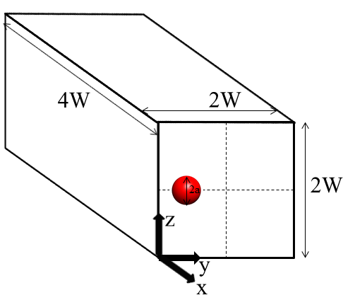
The active dominant forces on the migrating drop in the wall-normal direction are the inertial and deformation-induced lift and lateral drag forces. The direction of the inertial lift at drop locations far from the wall is towards it, and the deformation lift pushes the drop towards the channel center Zhang et al. 2016. The direction of the lateral drag is the negative of its migration velocity sign, assuming that the carrier fluid is stationary in the wall-normal direction Zhang et al. 2016. Therefore, if we assume the positive direction to be the one from the center to the wall, the force balance on the drop according to Newton’s second law is the following:
| (1) |
The drag force is computed based on its definition Ishii and Zuber 1979:
| (2) |
| (3) |
| (4) |
Where is the drag coefficient, is the relative velocity between the drop and the fluid (which is essentially its migration velocity), and is the frontal projected area of the drop. Equation 3 is consistent with the findings of Snyder et al. 2007; Ishii and Zuber 1979; Zhou et al. 2020; Kelbaliyev and Ceylan 2007; Salibindla et al. 2020 and those of Ceylan et al. 2001 at a viscosity ratio of one. Although eq. 3 is derived for steady flows, researchers have shown that the drag coefficient in unsteady flows depends heavily on an unsteady parameter that includes the density ratio Shao et al. 2017; Aggarwal and Peng 1995. Since the density ratio in the present study is one, the aforementioned unsteady parameter becomes zero, and hence, for unsteady flows (including oscillatory cases) can be approximated as the one for steady flows using this equation. The parameter is calculated based on the projected area of the drop on a plane having a normal vector parallel to its migration velocity. Thus, the value of this parameter varies at different instances. This procedure leads to a more precise computation of the drag force.
Considering a viscosity ratio of one, the deformation-induced lift for a drop that has a distance higher than its diameter from the closest wall leads to the following compact form Chan and Leal 1979; Stan et al. 2013:
| (5) |
Where is the drop capillary number, is the average velocity of the carrier fluid across the channel, and is the distance of the drop from the channel center. The linear dependency of this force with respect to the distance in the specified region is also confirmed in Rivero-Rodriguez and Scheid 2018.
The lift force analysis in this work is solely based on the drop trajectory. Therefore, to get a lift profile that spans a wide range of , the drop is released from two different initial locations:
- •
and (the upper release)
- •
and (the lower release)
The upper release is chosen such that the whole range of studied falls within the validity domain of the deformation force equation (eq. 5). This enables us to plug eq. 5 into the force balance equation (eq. 1) to get the inertial force once the total force is calculated as elaborated below. We will compare the inertial force at different values for the steady flows in the results section. The lower release initial location is slightly off from the channel center since it is also an equilibrium point, and if a drop is placed there, it does not move at all Chen et al. 2014. The initial component for both releases is on the main axis for faster convergence since the drop eventually focuses on the main axes according to our previous work Lafzi and Dabiri 2021. These different initial locations do not alter the drop equilibrium position Pan et al. 2016; Lan and Khismatullin 2012; Chaudhury et al. 2016; Razi and Pourghasemi 2017. The results of each parameter computation for both releases will be combined to reflect its overall behavior within the channel cross-section.
The migration velocity and acceleration of the drop is calculated by taking the first and second temporal derivatives from its trajectory numerically. Since time-step varies throughout the simulations to keep the Courant–Friedrichs–Lewy number at 0.9, the following equations are used to obtain the corresponding derivatives Sundqvist and Veronis 1970:
| (6) |
| (7) |
In which , , and and denote the distance from center and time at the current step. Both non-uniform finite difference schemes have a second-order accuracy.
Taking the first derivative from the steady flow trajectory at the lowest () results in a very noisy curve that is impossible to interpret. Therefore, we use an accurate non-linear regression by minimizing the sum of squared errors to fit the trajectories with analytical expressions, from which we can take first and second derivatives analytically. The trajectory from the upper release is very similar to an exponential decay. Therefore, we fit a curve with the following form to it:
| (8) |
Where , , and are all constants that should be determined after completing the optimization. The constant is essentially the drop equilibrium distance from the center. The trajectory from the lower release looks like the sigmoid logistic function. Consequently, we use the following equation as its analytical general form:
| (9) |
Where again, , , , and are the regressor constants. The regression fits to both trajectories from the upper and lower release have very high scores of 0.99 as plotted in fig. 2. This figure further confirms that the drop focuses at the same regardless of its initial location.

Once the migration acceleration is derived following the aforementioned steps, it will be multiplied by , which is the total constant mass of the drop with the initial spherical shape, to get the total force. By subtracting the calculated drag force from the total force, the total lift force can be obtained.
III Results and Discussion
In this section, we report the results of a single deformable droplet simulations in the previously introduced microchannel that contains both steady and oscillatory carrier fluid. As we are interested in studying the effects of oscillation frequency and Capillary number on the lift force, we fix the at a value of . ranges between and , and for oscillatory cases, values are chosen such that for a channel with a cross-section of and water as the working fluid at room temperature, the frequency ranges between 2Hz and 200Hz, which is mostly referred to in the literature Dincau et al. 2020. The validation of our numerical framework, as well as grid and domain independence studies, are discussed in detail in our previous work Lafzi and Dabiri 2021.
Figure 3 illustrates the dimensionless mass flow rate over dimensionless time. It can be seen that while the steady regime has the largest constant flow rate in a single direction, the average of oscillatory flow rates in each half of a periodic cycle decreases by increasing the frequency Lafzi et al. 2020; Lafzi and Dabiri 2021. Although the average of a sinusoidal function in half of a period is constant regardless of its oscillation frequency (), the lower maximum absolute value of the flow rate at higher frequencies is the chief reason for the observed phenomenon.

Figure 4 visualizes the dimensionless time-dependent frontal projected area of the droplet (parameter in equation 2) as it migrates toward its lateral equilibrium position traveling both upper and lower-release trajectories. The first thing we note is that in the transient stage before focusing, the drop has a higher average projected area while traveling the upper trajectory (fig. 4(b)) compared to the one in the lower trajectory (fig. 4(a)) in each of the flow regimes correspondingly. This is because the drop experiences more shear and deforms easier when traveling the upper trajectory. Moreover, in each subfigure, the average of is lower at a higher frequency since the average deformation parameter decreases by increasing the frequency Lafzi and Dabiri 2021. It is important to note that the minimum projected area of the drop in the steady flow is its initial value when the drop is still undeformed and has a spherical shape; in the oscillatory cases, this minimum value occurs when the direction of the flow changes in each periodic cycle. Also, as expected, the drop at higher deforms more and has a higher projected area. This is why is used for visualization here among all the other cases in the present study.


Figure 5 demonstrates the dimensionless total lift coefficient as a function of the dimensionless distance of the drop from the channel center in the steady flows and at different . Similar to Chen et al. 2014, all of the lift coefficients in this work are obtained by dividing the derived lift force, according to the introduced methodology in the previous section, by a factor of , in which is the average of flow velocity across the channel cross-section in the steady flow. As expected, we observe that each lift curve has a stable equilibrium point at the corresponding drop focal point. Furthermore, at each , the maximum positive total lift occurs when the drop migration velocity is also maximum. This maximum value is the highest at the lowest . In addition, the maximum negative total lift is at the initial location of the upper trajectory, and its absolute value is the highest for higher except for . This is because as we go further up from the channel center and the drop focal point, the deformation lift becomes the dominant force. According to equation 5, this force is larger at higher . Also, the negative lift sign in this region is due to the direction of the deformation-induced force, which is toward the center. The drop at is released from an initial location closer to the center compared to other cases because it has the highest deformability among all. When it was released from the same location as that of the others, it experienced an extremely large deformation that led to its break up. Therefore, the selected initial point for is the furthest possible one from the center that results in the largest possible deformation of the drop throughout its upper trajectory without its break up. Consequently, since the drop in this case starts to travel from a closer distance from the center, it has a lower maximum negative total lift compared to and (please refer to eq. 5 that shows the dependence of the deformation force on the drop distance from the center).

Since the principal hypothesis underlying equation 5 is that the wall effect is negligible due to the large distance of the drop from it Zhang et al. 2016; Ho and Leal 1974; Jahromi et al. 2019, we can assume that the shear-gradient force is the dominant component of the inertial lift in our study. After subtracting the calculated deformation lift based on this equation from the obtained total lift (fig. 5), we can derive the inertial lift, as shown in fig. 6. We see that the inertial lift coefficient increases as we increase the number. This could make sense as the more deformed shape of the drop can help further increase the difference between the relative velocities of the fluid with respect to the drop on the channel wall and center sides, which is the chief reason for the shear-gradient force existence Zhang et al. 2016. According to eq. 5, the deformation force is a linear function of the drop distance from the center and is larger for higher values of . Because of this trivial conclusion, a plot of this force is not depicted here.

Total lift curves acting on the drop in steady and different oscillatory flows at a few numbers are expressed in fig. 7. In each subfigure, the higher the drop migration velocity, the larger are both the amplitude of oscillations and the distance between two corresponding points (e.g. maximum or minimum in the oscillatory cycle) on two consecutive periodic cycles. Hence, similar to steady regimes, the maximum absolute values of oscillatory lift coefficients occur when the drop migration velocities are maximum as well. Similarly, the lift oscillations around the drop focal point and near the lower initial point are lower because the drop migration velocities are minimum at those locations.


The moving averages of the total lift coefficients in fig. 7 are plotted in fig. 8. The selected while computing the average of lift in each corresponding oscillatory cycle is chosen to be the middle value of in that period. Therefore, since oscillatory cycles with lower frequencies have longer periods, the averaged lift curves at lower frequencies cover a shorter length of (a later beginning and a sooner ending). We first note that the obtained averaged lift curves for the oscillatory flows are not necessarily as smooth as that of the steady lift at the corresponding . This observation becomes more pronounced as we increase or decrease . Nevertheless, these fluctuations on the curves are negligible compared to those of the original oscillatory lifts (fig. 7). Additionally, although the average of inertial and deformation-induced lift forces decrease separately by increasing Lafzi and Dabiri 2021, the difference between them (fig. 8) does not follow the same pattern. This confirms the existence of a drop focal point with an extremum distance from the channel center at an intermediate frequency, as elaborated in our previous work Lafzi and Dabiri 2021. Despite this, the average of lift is the largest in the steady flow and the smallest in the oscillatory flow with the highest frequency at each in our study.


By taking another close look at fig. 7, we realize that each of the oscillatory total lift coefficients can be fitted using an expression that comprises of a base curve, which can be best fitted by a 4th order polynomial, combined with the absolute value of some sinusoidal oscillations. Both the amplitude of oscillations and oscillatory periods can be controlled by the drop migration velocity and have direct relationship with it. In other words, the proposed expression can have the following form:
| (10) |
Where and are the time-dependent drop distance from the channel center and its migration velocity, respectively, and , , , , , , , , , and are the constants to be determined while performing the optimization. The constant is just placed for achieving higher accuracy for the fits, and it ends up to be almost zero compared to other constants in the expression. The resultant curves are plotted in fig. 9 against their corresponding data (fig. 7(a)) for and , , , and with scores of 0.99, 0.99, 0.99, and 0.97, respectively. Similar curves having the same proposed expression with scores of 0.97 or higher and capable of capturing all the infinitesimal details are obtained for other numbers as well.


To further extend the total lift prediction to more general cases within a continuous range of and , we consider the steady and averaged oscillatory lifts (fig. 8) for regression with a 4th order polynomial here. In other words, the expression in the first bracket of eq. 10 is replaced with a value of 1. Using the analytical set of equations 11, we can derive the unknown coefficients , , , , and of the polynomial analytically. In these equations, the subscripts for and denote their locations. For instance, the subscript max represents where the magnitude of total (or averaged) lift is maximum and its first derivative is zero. The obtained polynomials with this approach have scores of around 0.9 or higher for the cases presented in fig. 8.
| (11) |
Parameters , , , , , , and are already available for the cases in fig. 8 to solve the system of equations 11 for them. However, we use the multi-fidelity Gaussian processes (MFGP) method to predict these unknown parameters for any given double inputs of and . MFGP is a Bayesian stochastic approach that does a casual inference on a set of high and low-fidelity datasets, and it is extremely effective if there are strong correlations between them Perdikaris et al. 2017. This method is described in detail in our previous work, and it is carried out to predict the distance of the drop equilibrium position from the channel center with of 0.99 and root mean squared error (RMSE) of 0.01 in that work Lafzi and Dabiri 2021. Here, we refer to the data for the cases in fig. 8 except for as our high-fidelity data. We generate similar data for all the cases in that figure, but with a grid of in the , , and directions, respectively, and having 13038 triangular elements for the discretization of the drop. We consider this data as our low-fidelity dataset. Therefore, we have a total of 25 low and 20 high-fidelity data points, which satisfies the required nested structure to apply MFGP on the data Perdikaris et al. 2017. We randomly allocate 5 data points of the entire high-fidelity dataset as our test set since the high-fidelity response is our main target. We train the algorithm on the remaining 40 training data points and evaluate its performance on the test set. We repeat this procedure 30 times and compute the average of evaluation metrics so that the selection of test sets does not significantly affect the overall algorithm performance.
Table 1 presents the average of and RMSE on our 6 remaining unknown parameters after completing the aforementioned steps. We can see that the trained algorithm is capable of predicting the intended parameters with very high accuracies. Especially, the accurate prediction of and is useful for determining the maximum and minimum values of averaged total lift for any given input in the range, respectively. The slightly less accurate prediction for (i.e. where the maximum averaged lift occurs) is because of the present randomness in its values among different cases. This is unlike the consistent pattern that exists for other parameters for a combination of values across different numbers. The similar lower accurate prediction for is due to the lack of data points between and since all the cases with have the same upper release initial location. However, the score of around 0.8 for this prediction is still high, and it can help us determine the furthest starting point from the center and the widest traveling region of a droplet with in the microchannel so that it undergoes the largest possible deformation without breaking up.
| Parameter | RMSE | |
|---|---|---|
| 0.79 | 0.0140 | |
| 0.78 | 0.0213 | |
| 0.97 | 0.0007 | |
| 0.92 | 0.0177 | |
| 0.99 | 0.0015 | |
| 0.99 | 0.0003 |
IV Conclusions
The dynamics of particles and biological cells in microchannels has caught many researchers’ attention because of several biomicrofluidic applications it has. The underlying physics owes its behavior mainly to the presence of different lift forces in such channels. Hence, many scientists have dedicated their time to calculate or measure these forces. However, most of these works have focused on analyzing the lift forces acting on solid and non-deformable particles and studied the effects of parameters such as particles’ size, Reynolds number, etc on them. Consequently, such analysis on deformable droplets or bubbles and studying the effects of varying parameters like Capillary number is almost missing in the literature. In this work, we have extended such analysis to the case of a single deformable droplet in the channel. We have calculated the main components of the lift force based on a unique methodology that merely depends on the drop trajectory. To do so, first, the drop migration velocity and its frontal projected area as it travels its lateral trajectory have been computed to calculate the drag force in the wall-normal direction accurately. After applying Newton’s second law on the drop, the total lift profile is obtained over a region where the drop has a distance higher than its diameter from the wall. It has been observed that the total lift has a higher maximum at a lower Capillary, and its minimum decreases as we increase the . The inertial and deformation-induced lift forces both increase by increasing the number. Moreover, since the oscillatory flows within the microchannel were previously shown to enable working with sub-micron biological particles as well as introducing new focal points for them, we have also included these flow regimes in our analysis and investigated the effects of oscillation frequency on the lift in addition to the Capillary number. We have seen that for all cases, the total lift and for oscillatory ones, the amplitude of oscillations are both higher when the drop migration velocity is higher. At each , the steady lift and moving averages of oscillatory ones at different have also been compared. It has been shown that the steady lift has the largest magnitude, and the average of oscillatory one with the highest frequency in this study has the smallest strength. However, there is not a constant decreasing pattern in the average of lift by increasing the frequency, which is why the drop focuses furthest from the channel center at an intermediate . Additionally, an accurate mathematical expression has been proposed that captures the detailed total oscillatory lift curves at various with scores of 0.97 or higher. Finally, the multi-fidelity Gaussian processes has been used to accurately predict the 7 unknown parameters required to define a simple 4th order polynomial to fit the steady and averaged oscillatory lifts with scores of about 0.9 or higher for any given and within the ranges of and .
References
- Gossett et al. (2010) D. R. Gossett, W. M. Weaver, A. J. Mach, S. C. Hur, H. T. K. Tse, W. Lee, H. Amini, and D. Di Carlo, Analytical and bioanalytical chemistry 397, 3249 (2010).
- Toner and Irimia (2005) M. Toner and D. Irimia, Annu. Rev. Biomed. Eng. 7, 77 (2005).
- Gossett et al. (2012) D. R. Gossett, T. Henry, S. A. Lee, Y. Ying, A. G. Lindgren, O. O. Yang, J. Rao, A. T. Clark, and D. Di Carlo, Proceedings of the National Academy of Sciences 109, 7630 (2012).
- Karimi et al. (2013) A. Karimi, S. Yazdi, and A. Ardekani, Biomicrofluidics 7, 021501 (2013).
- Di Carlo (2009) D. Di Carlo, Lab on a Chip 9, 3038 (2009).
- Martel and Toner (2014) J. M. Martel and M. Toner, Annual review of biomedical engineering 16, 371 (2014).
- Bazaz et al. (2020) S. R. Bazaz, A. Mashhadian, A. Ehsani, S. C. Saha, T. Krüger, and M. E. Warkiani, Lab on a Chip 20, 1023 (2020).
- Connolly et al. (2020) S. Connolly, D. Newport, and K. McGourty, Biomicrofluidics 14, 031501 (2020).
- Stoecklein and Di Carlo (2018) D. Stoecklein and D. Di Carlo, Analytical chemistry 91, 296 (2018).
- Di Carlo et al. (2009) D. Di Carlo, J. F. Edd, K. J. Humphry, H. A. Stone, and M. Toner, Physical review letters 102, 094503 (2009).
- Prohm and Stark (2014) C. Prohm and H. Stark, Lab on a Chip 14, 2115 (2014).
- Su et al. (2021) J. Su, X. Chen, Y. Zhu, and G. Hu, Lab on a Chip (2021).
- Wang et al. (2017) Q. Wang, D. Yuan, and W. Li, Micromachines 8, 197 (2017).
- Asmolov et al. (2018) E. S. Asmolov, A. L. Dubov, T. V. Nizkaya, J. Harting, and O. I. Vinogradova, Journal of Fluid Mechanics 840, 613 (2018).
- Liu et al. (2016) C. Liu, C. Xue, J. Sun, and G. Hu, Lab on a Chip 16, 884 (2016).
- Zastawny et al. (2012) M. Zastawny, G. Mallouppas, F. Zhao, and B. Van Wachem, International Journal of Multiphase Flow 39, 227 (2012).
- Mannan and Leiderman (2020) F. O. Mannan and K. Leiderman, Physical Review Fluids 5, 044102 (2020).
- Chen et al. (2014) X. Chen, C. Xue, L. Zhang, G. Hu, X. Jiang, and J. Sun, Physics of Fluids 26, 112003 (2014).
- Rivero-Rodriguez and Scheid (2018) J. Rivero-Rodriguez and B. Scheid, Journal of Fluid Mechanics 855, 1242 (2018).
- Stan et al. (2011) C. A. Stan, L. Guglielmini, A. K. Ellerbee, D. Caviezel, H. A. Stone, and G. M. Whitesides, Physical Review E 84, 036302 (2011).
- Zhou and Papautsky (2013) J. Zhou and I. Papautsky, Lab on a Chip 13, 1121 (2013).
- Raffiee et al. (2019) A. H. Raffiee, A. M. Ardekani, and S. Dabiri, Journal of Non-Newtonian Fluid Mechanics 272, 104166 (2019).
- Schaaf and Stark (2017) C. Schaaf and H. Stark, Soft Matter 13, 3544 (2017).
- Mutlu et al. (2018) B. R. Mutlu, J. F. Edd, and M. Toner, Proceedings of the National Academy of Sciences 115, 7682 (2018).
- Lafzi et al. (2020) A. Lafzi, A. H. Raffiee, and S. Dabiri, Physical Review E 102, 063110 (2020).
- Schonewill (2008) P. P. Schonewill, Oscillatory Flow: Effect on Transverse Diffusivity and Inertial Migration of Particles and Bubbles, Ph.D. thesis, University Of Notre Dame (2008).
- Unverdi and Tryggvason (1992) S. O. Unverdi and G. Tryggvason, Journal of computational physics 100, 25 (1992).
- Lafzi and Dabiri (2021) A. Lafzi and S. Dabiri, Physics of Fluids 33, 062010 (2021).
- Zhang et al. (2016) J. Zhang, S. Yan, D. Yuan, G. Alici, N.-T. Nguyen, M. E. Warkiani, and W. Li, Lab on a Chip 16, 10 (2016).
- Ishii and Zuber (1979) M. Ishii and N. Zuber, AIChE journal 25, 843 (1979).
- Snyder et al. (2007) M. R. Snyder, O. M. Knio, J. Katz, and O. P. Le Maître, Physics of Fluids 19, 065108 (2007).
- Zhou et al. (2020) Y. Zhou, C. Zhao, and H. Bo, International Journal of Multiphase Flow 127, 103265 (2020).
- Kelbaliyev and Ceylan (2007) G. Kelbaliyev and K. Ceylan, Chemical Engineering Communications 194, 1623 (2007).
- Salibindla et al. (2020) A. K. Salibindla, A. U. M. Masuk, S. Tan, and R. Ni, Journal of Fluid Mechanics 894 (2020).
- Ceylan et al. (2001) K. Ceylan, A. Altunbaş, and G. Kelbaliyev, Powder technology 119, 250 (2001).
- Shao et al. (2017) C. Shao, K. Luo, and J. Fan, Chemical Engineering Journal 308, 619 (2017).
- Aggarwal and Peng (1995) S. Aggarwal and F. Peng, (1995).
- Chan and Leal (1979) P.-H. Chan and L. Leal, Journal of Fluid Mechanics 92, 131 (1979).
- Stan et al. (2013) C. A. Stan, A. K. Ellerbee, L. Guglielmini, H. A. Stone, and G. M. Whitesides, Lab on a Chip 13, 365 (2013).
- Pan et al. (2016) D.-y. Pan, Y.-q. Lin, L.-x. Zhang, and X.-m. Shao, Journal of Hydrodynamics 28, 702 (2016).
- Lan and Khismatullin (2012) H. Lan and D. B. Khismatullin, International journal of multiphase flow 47, 73 (2012).
- Chaudhury et al. (2016) K. Chaudhury, S. Mandal, and S. Chakraborty, Physical Review E 93, 023106 (2016).
- Razi and Pourghasemi (2017) M. Razi and M. Pourghasemi, Computers & Fluids 154, 200 (2017).
- Sundqvist and Veronis (1970) H. Sundqvist and G. Veronis, Tellus 22, 26 (1970).
- Dincau et al. (2020) B. Dincau, E. Dressaire, and A. Sauret, Small 16, 1904032 (2020).
- Ho and Leal (1974) B. Ho and L. Leal, Journal of fluid mechanics 65, 365 (1974).
- Jahromi et al. (2019) S. Jahromi, E. Amani, and S. Movahed, Electrophoresis 40, 1678 (2019).
- Perdikaris et al. (2017) P. Perdikaris, M. Raissi, A. Damianou, N. Lawrence, and G. E. Karniadakis, Proceedings of the Royal Society A: Mathematical, Physical and Engineering Sciences 473, 20160751 (2017).