Stellar kinematics of dwarf galaxies from multi-epoch spectroscopy: application to Triangulum II Thanks: New observations reported here were obtained at the MMT Observatory, a joint facility of the Smithsonian Institution and the University of Arizona. Some of the data presented herein were obtained at the W. M. Keck Observatory, which is operated as a scientific partnership among the California Institute of Technology, the University of California and the National Aeronautics and Space Administration. The Observatory was made possible by the generous financial support of the W. M. Keck Foundation.2021Stellar kinematics of dwarf galaxies from multi-epoch spectroscopy: application to Triangulum II–4
Abstract
We present new MMT/Hectochelle spectroscopic measurements for 257 stars observed along the line of sight to the ultra-faint dwarf galaxy Triangulum II. Combining results from previous Keck/DEIMOS spectroscopy, we obtain a sample that includes 16 likely members of Triangulum II, with up to 10 independent redshift measurements per star. To this multi-epoch kinematic data set we apply methodology that we develop in order to infer binary orbital parameters from sparsely sampled radial velocity curves with as few as two epochs. For a previously identified (spatially unresolved) binary system in Tri II, we infer an orbital solution with period , semi-major axis , and systemic velocity that we then use in the analysis of Tri II’s internal kinematics. Despite this improvement in the modeling of binary star systems, the current data remain insufficient to resolve the velocity dispersion of Triangulum II. We instead find a 95% confidence upper limit of .
Keywords:
(stars:) binaries: spectroscopic – galaxies: kinematics and dynamics1 Introduction
Dwarf galaxies are of great importance for astrophysics. From a galaxy formation perspective, dwarf galaxies are among the oldest and least chemically evolved objects (Mateo 1998; Tolstoy et al. 2009; McConnachie 2012). From a dark matter perspective, they include the most dark matter dominated systems known, with published dynamical mass-to-light ratios reaching as high as in solar units (Simon 2019, and references therein). In this vein, dwarf galaxies are believed to be key components in unpacking the mystery of dark matter, as they probe the small-scale structure (< 1 Mpc) regime of CDM cosmology (Bullock & Boylan-Kolchin 2017).
In order to place dwarf galaxies into their proper cosmological context, we must obtain accurate estimates of their dark matter content. The simplest dynamical mass estimators, based on the assumption of dynamic equilibrium, are functions of the effective radius and line-of-sight velocity dispersion measured for the stellar component (Illingworth 1976; Walker et al. 2009; Wolf et al. 2010; Errani et al. 2018, e.g.,). However, measurements of the stellar velocity dispersion can be challenging. One reason is the small number and low luminosities of stellar tracers in especially the ‘ultrafaint’ dwarf galaxies. Another challenge is the existence of unresolved binary stars, whose orbital motions add a time-dependent component to the velocities measured for individual stars, and—if unaccounted for—can thereby inflate measurements of dwarf galaxy velocity dispersions. Binary orbital motions alone can generate apparent velocity dispersions of a few km s-1 (McConnachie & Côté 2010). While this effect is negligible for the more luminous dwarf spheroidals, which have intrinsic velocity dispersions of km s-1 (Olszewski et al. 1996), it can potentially contribute significantly to the km s-1 dispersions observed for the least luminous galaxies (McConnachie & Côté 2010; Minor et al. 2010).
Various strategies have been used to account for the effect of binary stars on velocity dispersions and the dynamical masses derived therefrom. When multi-epoch spectroscopy is available, one can identify probable binary systems via their observed accelerations (Olszewski et al. 1996; Martinez et al. 2011; Koposov et al. 2011; Minor et al. 2019, e.g.,); indeed modeling of multi-epoch spectroscopic data sets for luminous dwarf spheroidals suggests typical binary fractions near (Minor 2013; Spencer et al. 2017; Spencer et al. 2018), consistent with studies of Galactic binaries that indicate relatively high multiplicity fractions at low metallicity (Badenes et al. 2018). In some cases, the removal of suspected binary stars has a significant impact on the measured velocity dispersion (Kirby et al. 2017; Venn et al. 2017, e.g.,).
The Triangulum II (Tri II) ultra-faint dwarf galaxy provides an interesting case study. The original kinematic study of Tri II, based on single-epoch spectroscopy of six member stars, measured a velocity dispersion of , suggesting a dynamical mass-to-light ratio of in solar units, and an extremely high dark matter density of (Kirby et al. 2015). An independent study by Martin et al. 2016 obtained a spectroscopic sample of 13 member stars, finding complicated kinematics in which a central velocity dispersion of gives way to a larger value of km s-1 at a large radius. Both studies found evidence for nonzero metallicity dispersion, supporting the conclusion that Tri II is a dwarf galaxy embedded in a massive dark matter halo, and not a self-gravitating star cluster.
However, follow-up spectroscopy soon provided a time domain and revealed the presence of at least one star with significant velocity variability. From high-resolution spectra obtained primarily to analyze chemical abundances, Venn et al. 2017 measured a change in velocity for one star (Star46) of km s-1 with respect to the initial epoch measured by Martin et al. 2016. Kirby et al. 2017 added additional epochs for this star, independently confirming its velocity variability and finding that, when they excluded the likely binary from their analysis, the velocity dispersion was unresolved. These circumstances leave the case for a dominant dark matter halo in Tri II resting on the indirect argument provided by its metallicity spread (Venn et al. 2017).
Here, we add to the saga of Tri II in two ways. First, we present new spectroscopic data acquired with the Hectochelle spectrograph at the 6.5-m MMT. Second, we combine with the previously published spectroscopic data in order to obtain a multi-epoch data set that then lets us model the orbital parameters of the likely binary star. Our orbital solution includes an inference for the binary system’s center-of-mass motion, allowing us properly to include this star in our analysis of Tri II’s stellar kinematics.
To date, only one star system within a dwarf spheroidal galaxy has a full orbital solution, based on 34 independent velocity measurements taken over a two-year baseline (Koch et al. 2014). Here, we develop methodology for inferring orbital solutions with as few as two velocity epochs. The problem of finding orbital parameters for a binary system given a small number of radial velocity (RV) measurements has been undertaken previously by Price-Whelan et al. 2017 to create the JOKER. Like the JOKER, the binary model we present in this paper takes the approach of performing rejection sampling with likelihood function marginalized over some orbital parameters. However, our method has the added modifications such as the marginalization over inclination rather than semi-amplitude (allowing for the calculation of semi-major axis), the ability to take non-trivial priors over binary parameters, and using parameter samples for hierarchical models of binary populations.
In the next section we discuss the MMT and Keck catalogues used in this analysis as well as the calculation of a zero-point correction between the two instruments. In section 3 we present our methodology for modeling of binary and non-binary star systems as well as the galaxy kinematics. We then detail the resulting orbital parameter for the Tri II binary system and the overall Tri II kinematics in section 4. Lastly, we discuss the findings from our work in Section 5 and we suggest a hierarchical model building off the methods used.
2 Data
2.1 MMT Hectochelle
During Dec. 2015 and Oct. - Nov. 2016, we acquired new spectra of stars in Tri II using the Hectochelle spectrograph (Szentgyorgyi et al. 2011) at the 6.5-m MMT Observatory on Mt. Hopkins, Arizona. Hectochelle deploys up to 240 optical fibers, each with aperture arcsec, over a field of diameter . We observed using the ‘RV31’ filter, isolating the wavelength range of at resolution .
We observed five different Hectochelle fiber configurations, each centered on the published center of Tri II, allowing us to observe up to unique targets, with many stars included in multiple targeting configurations.
To clean the overwhelming contamination from foreground Milky Way stars, we rely on narrow-band, metallicity sensitive CaHK observations of Tri II. The observations follow a similar strategy and goal as presented by Starkenburg et al. 2017 in the Pristine survey but correspond to a single CFHT MegaCam field centered on Tri II. The field covers the full extent of Tri II and the integration amount to 4,800 s in total from the CaHK images. Additional observations were also obtained in the MegaCam g and i bands (4,140 and 4,050 s, respectively) to benefit from the full depth of the CaHK photometry is deeper than the Pan-STARRS1 data that were used to discover Tri II (Laevens et al. 2015). All were observed in service mode by the CFHT observing staff between 2015-07-18 and 2016-02-13. After pre-processing of the images with ELIXIR by CFHT (Magnier & Cuillandre 2004, de-biasing, flat-fielding, and de-trending;), the images were astrometrically calibrated, stacked, and processed for photometry with the CASU pipeline (Irwin & Lewis 2001), as described in detail by Starkenburg et al. 2017. The broadband and photometry is calibrated onto the Pan-STARRS1 and bands and we directly use the Pan-STARRS1 photometry at the bright end, where the CFHT observations saturate. Finally, the photometric catalog is de-reddened using the Schlegel, Finkbeiner and Davis dust maps.
Similarly to what was done for the Pristine Inner Galaxy Survey (Arentsen et al. 2020) the large number of science fibers available on Hectochelle allowed us to perform a broad selection of targets in the part of the CaHK color-color diagram that contains metal-poor stars. This allowed us to bypass any potential calibration issue and the use of Pan-STARRS1 broad-band magnitudes instead of the SDSS ones we relied on in Starkenburg et al. 2017. In particular, we selected stars based on their color-magnitude diagram location so they broadly follow an old and metal-poor isochrone. In the color-color space using CaHK that is presented in Figure 1 and used by the Pristine survey, we loosely select stars from the metal-poor region, using known Tri II members as a guideline to isolate other stars with similar properties. Once fibers are assigned to these high-priority stars, we fill the rest of the fibers with random CMD-selected stars, irrespective of their CaHK information.
We processed all raw Hectochelle spectra using the CfA pipeline (HSRED v2.111 1 https://bitbucket.org/saotdc/hsred/ ). Following the procedure described in detail by Walker et al. 2015, we then analyzed each individual spectrum by fitting a model based on a library of synthetic template spectra that span a regular grid in effective temperature, surface gravity and [Fe/H] metallicity. In addition to the stellar-atmospheric parameters, we fit for line-of-sight velocity as well as several free parameters that specify the continuum shape and correct for wavelength-dependent velocity shifts.
With respect to the procedure documented by Walker et al. 2015, for present purposes we update our estimation of systematic errors associated with line-of-sight velocity and metallicity. For this task we use our entire catalog of MMT/Hectochelle observations of dwarf galaxies and globular clusters, including observations spanning the years 2005 to 2020. This sample includes 12517 independent observations of 7906 unique stars, including 2501 stars with up to 13 individual measurements. We model the pair-wise velocity and metallicity differences as a mixture of a Gaussian with an outlier model (see Section 4.1 of Li et al. 2019 and Section 2.2 of Pace et al. 2021).The final uncertainty () is treated as a systematic error () plus a scaling parameter () and . We find and km s-1for the velocity systematic errors, and and for metallicity systematic errors.
2.2 Keck DEIMOS
Our sample also includes spectroscopy obtained with the Deep Extragalactic Imaging Multi-Object Spectrograph (Faber et al. 2003, DEIMOS;). First, Kirby et al. 2015; Kirby et al. 2017 observed six slitmasks in 2015 and 2016. They used the 1200G grating, which achieves a spectral resolution of at 8500 Å, in the spectral vicinity of the Ca ii infrared triplet. Second, Martin et al. 2016 observed two DEIMOS slitmasks with a similar spectral configuration as Kirby et al. 2015
Kirby et al. 2015 selected stars using Keck/LRIS (Oke et al. 1995) photometry. They chose a generous selection region in the CMD around the red giant branch as defined by the ridgeline of the globular cluster M92. Martin et al. 2016 used a similar selection technique with photometry (Laevens et al. 2015) from the Large Binocular Camera. In general, the field of Tri II is sparse enough that most candidate member stars in the field of the slitmask could be observed. As a result, the samples have little selection bias due to color (or stellar age or metallicity). Kirby et al. 2017 were mainly interested in quantifying radial velocity variability, not in finding new members. As a result, they designed their slitmasks to target stars already identified as members by Kirby et al. 2015 and Martin et al. 2016.
Velocities were measured in slightly different ways. Kirby et al. 2015; Kirby et al. 2017 reduced the spectra with custom modifications to the spec2d data reduction pipeline (Cooper et al. 2012). They matched empirical spectral templates observed with DEIMOS to the Tri II spectra and varied the velocity until was minimized. Martin et al. 2016 used their own custom pipeline (Ibata et al. 2011) to reduce the spectra. They determined radial velocities from the mean wavelengths of Gaussian fits to the Ca ii triplet.
Slit imaging spectrographs can experience radial velocity zero-point shifts if the star is not perfectly centered in the slit. This effect can be mitigated by observing the wavelengths of telluric absorption lines (Sohn et al. 2007, e.g.,). The slit centering correction is taken to be the deviation of the wavelengths of these lines from the geocentric rest frame. All of the studies used in this work performed such a correction.
2.3 Zero-point offset
In this section, we describe the calculation of the zero-point velocity offset between Keck and MMT. Although our complete set of Tri II Keck observations is a concatenation of the Kirby et al. 2017 and Martin et al. 2016 datasets, the zero-point offset between the two appears consistent with zero (Kirby et al. 2017, see Section 3.2 of). For this analysis, we have defined the offset as the MMT zero-point minus the Keck zero-point. There are 8 objects in our dataset around the Tri II galactic center with radial velocity measurements in both MMT and Keck catalogues. Measurements for a given object and instrument are combined into a single weighted mean value. We then calculate the offset between the sets of combined instrument velocities assuming Gaussian errors.
The methods described here and in section 3 are based on a Gaussian likelihood function, which is described in terms of model prediction , model error , given data in the form of the observed velocity :
| (1) |
This is the general likelihood for a given velocity prediction, and the total likelihood function is the product of the velocity likelihoods.
In the context of finding a zero-point offset, we apply this likelihood to a set of velocity differences , where represents the difference between the th star’s MMT weighted mean velocity and its Keck weighted mean velocity, . We assume that these velocity differences are consistent with the zero-point offset between instruments and that there is no dispersion in , only observational errors. Thus, the total likelihood is the product of the likelihoods of individual objects, .
However, some objects have a very large velocity difference between the instruments, possibly due to low signal-to-noise or unconfirmed binarity. A convenient way to account for these objects is to construct a mixture model to treat them as outliers, a similar model is used in Li et al. 2019. The new likelihood for a given object is the sum of the original Gaussian likelihood and outlier model likelihood weighted by the probability the object is an outlier. The new likelihood is written as…
| (2) |
where represents the outlier fraction and represents the offset correction. The outlier model is applied to the difference in the combined weighted mean velocities for each instrument and is taken to be a Gaussian with a large standard deviation. The priors are as follows:
- •
offset : uniform(, )
- •
outlier fraction : uniform(0, 0.5)
- •
outlier model standard deviation : uniform(, )
We define the posterior as the Gaussian likelihood multiplied by our set of priors and look for a that maximizes this posterior. The offset error is taken as the width of this offset posterior distribution. We derive the offset value from the resulting posterior, sampled using Markov Chain Monte Carlo (MCMC) by the Metropolis–Hastings algorithm via the emcee python package (Foreman-Mackey et al. 2013). Applying this procedure to the 8 stars in the overlapping MMT-Keck datasets observed around the Tri II galactic center, we find an offset value of . While this value could be determined using only our Tri II dataset, the large error means that the offset is not resolved within and the introduction of a large offset error can make it more difficult to resolve the Tri II velocity dispersion.
To improve the error on our zero-point offset between the instruments, we also include Keck/DEIMOS (Pace et al. 2020) and MMT/Hectochelle (Spencer et al. 2018) observations from an additional 288 Ursa Minor objects. The combined Tri II and Ursa Minor dataset results in an offset correction of .
We opt to use the offset that is calculated while including Ursa Minor observations, as the larger amount of data gives a more precise value for the offset. Thus, we bring all observations onto a common zero-point by subtracting a fixed amount of from each velocity measurement obtained with Keck/DEIMOS. We do not propagate the offset error as the total error is dominated by the combination of instrument-specific systematics and random errors.
2.4 Membership
To determine Tri II membership, we sigma clip our dataset at from both the galaxy mean line-of-sight velocity and proper motion. This step removes objects whose observations differ from the Tri II measurements times the root sum of the squared of the galaxy and measurement errors, . We use the proper motions from Gaia eDR3 (Gaia Collaboration et al. 2021, Figure 2). All members are consistent with zero parallax (i.e, ). The Tri II mean velocity is taken as (Kirby et al. 2017) and the galaxy proper motion as (Pace et al. 2022). Other systemic proper motion measurements with Gaia EDR3 find similar results (McConnachie & Venn 2020; Battaglia et al. 2022). While the velocity dispersion is unresolved, we use (Figure 3). Our resulting sample consists of 16 member stars, one of which is the previously confirmed binary star (GAIA ID 331086526201161088 which we refer to as Star46 or MIC2016-46 in this work). There is one star that is observed by MMT only, two stars in the overlap of MMT and Keck, and the remaining 13 are observed by Keck only.
Figure 4 shows the location of our final sample of member stars on a color-magnitude diagram compared to all the stars within the Tri II half light radius after a star-galaxy separation cut observed by the Subaru/Hyper Suprime-Cam (Miyazaki et al. 2018, HSC;) and Pan-STARRS1 (Flewelling et al. 2020). The isochrone parameters and the half-light radius (2.5′) are taken from Carlin et al. 2017. In Figures 2, 3, and 4, we indicate the locations of the binary star (Star46) and another member, called Star31 (or MIC2016-31) in this analysis, with black markers of different shapes. Star31 is specifically marked because of its uncertainty as a member in Kirby et al. 2017 (also called Star31 in their work). Its membership is brought into question due to it being (1) far from the galactic center, (2) the most metal rich star in the sample (to the point of driving Tri II’s [Fe/H] dispersion), and (3) the only star whose velocity is from the galaxy mean velocity. However, the now available Gaia eDR3 indicate its proper motion is consistent with Tri II, bolstering its case as a member.
3 Methods
3.1 Binary Stars
When a star is a part of a binary system, the orbital motion can give rise to periodic variability in the line-of-sight velocity. If one star is much brighter than its companion (e.g., a red giant with a main sequence companion), then a single-epoch spectrum may not show any evidence of variability. Conventional methods of combining observations, such as a weighted mean, can misrepresent the true systemic velocity if the system is sparsely observed and/or it results in an inflated error in the combined velocity. Thus, binary stars can directly inflate the calculated velocity dispersion if not accounted for properly. Though the true line-of-sight velocity will vary with time, it will oscillate around the center-of-mass (systemic) velocity.
In terms of the true anomaly (angular position in the orbital plane from the periastron direction), argument of periapsis (angle in the orbital plane between the ascending node and the periastron) and systemic velocity , a member of a binary star system has line-of-sight velocity that varies with time according to…
| (3) |
(Murray & Correia 2010). We can further expand the semi-amplitude in terms of the binary parameters, period , semi-major axis , inclination , and eccentricity as
| (4) |
This is the model that we use to fit the observed radial velocity curves. It is worth mentioning that instead of using as a free parameter, we sample in , representing the phase, which is related to a constant called the time of periastron passage, , by a factor of . We can relate and using the eccentricity anomaly, .
| (5) |
| (6) |
We furthermore include a jitter parameter that acts as secondary error to account for velocity variability not due to periodic orbital motion. We note that Hekker et al. 2008 found a correlation between velocity jitter and surface gravity for red-giant branch stars, where stars with can have excess jitter . However, the majority of our members, including Star46, exist on the lower red giant branch where . This is commonly the case for stars in ultra-faint dwarfs, so there is little concern that internal mechanisms will inflate the galaxy velocity dispersion.
We continue to assume a Gaussian error on velocity measurements, thus allowing us to use the previously defined Gaussian likelihood function, equation 1. We generate samples of the posterior on the orbital binary parameters using rejection sampling. This sampling is carried out over the course of iterations, with each iteration starting with points before rejection. After rejection, the surviving samples across all iterations are combined. The choice to use rejection sampling instead of Monte-Carlo-Markov-Chain (MCMC) is due to the potential multi-modality posterior. A sparsely observed binary can have multiple possible orbital period solutions, which have corresponding total mass and systemic velocity values, represented as peaks in the posterior. This specific scenario can lead to untouched areas of the posterior when using MCMC.
The priors are quite uninformative, which ensures that we can fully sample all the possible binary parameters. Note that there is a pre-defined mass range, such that the prior in total mass is loguniform from to , which is used to bound the semi-major axis prior. The priors on all angles are uniform. We adopt the uniform prior on corresponding to a random orientation of binary orbits and a Beta distribution for eccentricities. The parameters for the Beta distribution are and , resulting in a near uniform between 0 and 1 for eccentricities, . For compactness, we explicitly state the priors on each of the orbital parameters alongside the resulting Star46 binary parameter posteriors in Table 1.
| Binary Star Orbital Parameters | |||
|---|---|---|---|
| Parameter | Prior | Short Per. | Long Per. |
| Period | linearly decreasing in log() from 1 day to days | days | days |
| Eccentricity | Beta(1.5,1.5) | ||
| Systemic velocity | Normal(0,) | ||
| Phase | uniform(0,2) | ||
| Argument of periapsis | uniform(0,2) | ||
| Jitter | Normal( | ||
| Semi-major axis | loguniform, bounds determined from mass | AU | AU |
| Inclination | uniform(0,2) in | ||
We are able to make further assumptions about the system by modifying the surviving posterior samples. We remove nonphysical solutions corresponding to close binaries where the pericenter is less than the stellar radius or where the mass of the companion star is negative. These stellar radii and masses are calculated using the Isochrones python package (Morton 2015) to determine stellar parameters for the binary star of age 13 Gyr, [Fe/H] of -2.2, and distance modulus of 17.24 using the MESA Isochrones and Stellar Tracks (MIST) grid (Dotter 2016; Choi et al. 2016). Figure 4 shows the relevant isochrone fit on a color-magnitude diagram with Tri II members plotted. For the binary star Star46, we determine a mass of and stellar radius of from an isochrone fit to Tri II stars. We equivalently derive a mass and radius for the other Tri II members by finding the point on the isochrone closest to each member star using the same steps.
Similarly, Raghavan et al. 2010 looked at 259 confirmed solar-type binaries in the Hipparcos catalog and found that the periods are distributed according to a log-normal distribution with and standard deviation , where is in days. This is a more informative prior on the period than our default period prior. We refer to this lognormal distribution as the "Raghavan prior" for the remainder of this paper. We present this distribution with the minor caveat that most of the detectable member stars of dwarf galaxies are not solar-type (main-sequence) stars, but rather red giant branch stars.
We are able to infer the posterior under this prior by re-sampling from the current surviving samples with non-uniform weights. These weights are proportional to the ratio of the Raghavan period distribution to the default prior. All of these assumptions shift the posterior away from shorter orbital periods, but as we will see in section 4.2, the application of this prior on Star46 significantly alters the parameter posterior. As such, we present the results both before and after the application of the Raghavan prior.
3.2 Non-Binary Stars
In the case of non-binary stars, we expect line-of-sight velocity observations to be consistent with a constant velocity model with some scatter in each measurement proportional to the observational error. Our goal is to determine a star’s true velocity by combining multiple epochs of radial velocity measurements into one stellar velocity. A common approach to this is calculating the weighted mean—i.e., summing the measurements weighted by the inverse of the squared errors. This approach has the benefits of being analytic and thus not computationally intensive. However, it has the downside of underestimating the error when dealing with potentially variable systems. In this section, we offer another method to calculate the true stellar velocity by finding its posterior distribution.
Once again, the assumption of Gaussian error allows us to use the previously defined Gaussian likelihood function, equation 1, and a set of priors in true velocity and velocity error to sample from the true velocity posterior. The sampling is done using MCMC sampling and is performed with 24 walkers, 1000 steps each, and 100 step burn-in. For a set of line-of-sight velocity observations with errors , we define a uniform prior in true velocity that is non-zero from to . We also use Jeffrey’s prior for the standard deviation of a Gaussian distribution ( or uniform in ) for the true velocity error. The error of the combined velocity measurement is taken as one standard deviation from the posterior on the mean. We use the mixture sub package found in scikit-learn (Pedregosa et al. 2011) to fit a Gaussian mixture model (GMM) of a singular Gaussian to the resulting posterior samples. Figure 5 shows the radial velocity curve and resulting posteriors using this method, referred to as the Gaussian fit method, and binary model method for an example Tri II member star with multiple velocity observations.
This Gaussian Fit method has the advantage in that it does not assume binarity but does retain increased error with larger variability in the RV curve, more than the weighted mean. For comparison, we also calculate the combined velocities under the weighted mean and binary model methods (Figure 6). Applying the binary model to the, assumed non-binary, member stars takes up significantly more computation time and results in a larger uncertainty in the combined velocity. Over short time-scales, the observations can be consistent with either a constant velocity model or the RV curve of a long period binary. These methods are only applied to members with more than one velocity measurement as neither would be informative for stars with only a single epoch. Using the Gaussian Fit method would be the equivalent of trying to fit a Gaussian distribution to a single point. For the binary model, there is not enough information in a single epoch to restrict the possible binary solutions.
3.3 Mean Velocity and Velocity Dispersion
The Tri II velocity dispersion can be inferred from the posterior using the same Gaussian likelihood function as in previous sections (Equation 1). We define another Gaussian model in terms of the mean velocity and the velocity dispersion of the galaxy. The total likelihood is the product of the likelihood of the model on the stellar velocity of each member. For stars with multiple velocity measurements, the measured velocities are combined using one of the methods presented in the previous sections. In the case of a multi-modal posterior, such as for Star46, we must fit a one-dimensional GMM to the systemic velocity posterior and the likelihood for that object becomes…
| (7) |
where and represent the mean and weight of the th Gaussian in the mixture model with Gaussians. The error on is taken as the standard deviation of the Gaussian and the number of Gaussians in the GMM is determined by manually inspecting the posterior. Figure 7 shows the GMM fits to the Star46 systemic velocity posterior before and after the application of the Raghavan prior.
The velocity dispersion prior is log-uniform from to , which is equivalent to Jeffrey’s prior. The minimum value corresponds to the case where the galactic dynamics are fully determined by visible matter (see Appendix A). We have chosen to find the posterior of rather than to better sample smaller velocity dispersion values. Once again, we use a uniform prior from to as our prior on mean velocity.
4 Results
4.1 Binary Orbital Parameters
Within our data set, we are able to spectroscopically identify one star, Star46, as a binary. Attempting to fit a constant velocity model to the observations of this object, we find a reduced chi-squared of . Previous analyses by Venn et al. 2017 and Kirby et al. 2017 found this star to be part of a binary system. For comparison, the member with the second highest reduced chi-squared is MIC2016-27 with . Although this value could suggest possible binarity for MIC2016-27, its velocity variations are more consistent with a constant-velocity model than Star46.
In this analysis, we use the 4 velocity measurements of this star from MMT (Table 3) and 5 from Keck (Table 4). There are two additional velocity measurements made in Geminin/GRACES data (Venn et al. 2017; Ji et al. 2020) that we have opted to not use for two reasons. First, the inclusion of this data would add an additional unknown zero-point correction that is more difficult to quantify due to less overlap in number of stars. Second, we have explored including them and found that they do not impact the resulting orbital parameter posterior (See Appendix B).
After an initial pass with our model on Star46, we find that there are two noticeable peaks in the posterior corresponding to periods of 0.4 and 0.8 years. We are able to eliminate the sub-harmonics (e.g., 0.2, 0.1 years) from our restrictions on pericenter and Kepler’s third law both limiting the allowed semi-major axis values. Because the period modes are distinct, we re-run the sampling with a more restricted period prior bound at 0.3 and 0.95 years to ensure a larger number of surviving posterior samples. The resulting binary orbital parameters presented in this section are derived from the posterior after removing samples that correspond to a negative companion mass but before the application of the Raghavan prior. Figure 8 is a corner plot of the posterior of select parameters and shows two distinct peaks corresponding to long and short period solutions. We separate the posterior samples at the 0.6 year boundary and present the orbital parameter values taken from the truncated posteriors in Table 1. Figure 9 shows the RV curve for this star, as well as the orbital solutions that correspond to the surviving samples.
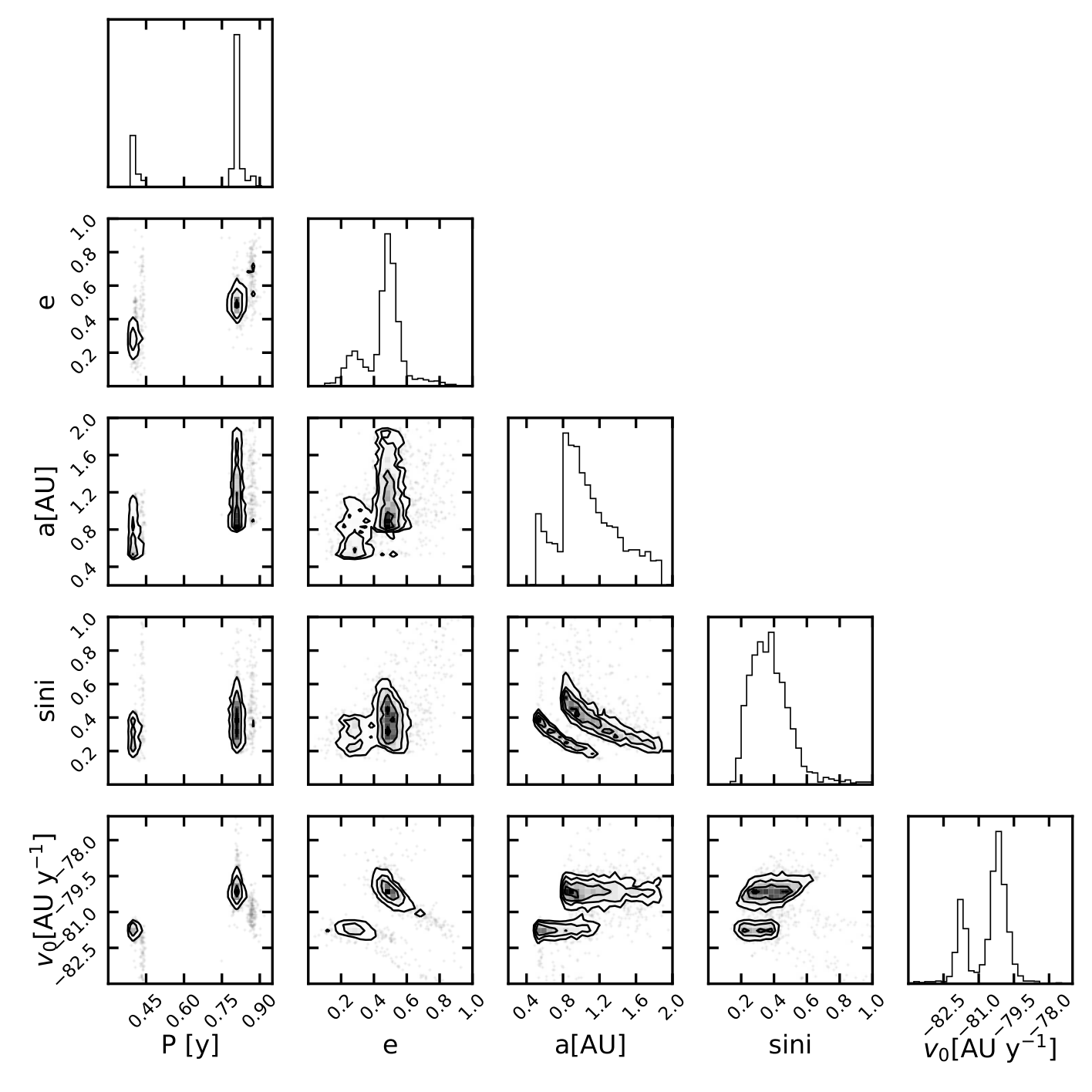
The posteriors of the semi-major axis for both solutions are consistent with values less than , indicating that this is a close binary. The resulting overall binary parameter space is that of a common binary star system. The companion mass posterior is not distinct enough from the prior to be informative, but all of the samples correspond to stellar masses potentially on the main sequence.
For comparison, the only other binary star in an ultra-faint dwarf spheroidal, Her-3 in the Hercules dwarf, has a smaller eccentricity () and period () values (Koch et al. 2014). Plugging into equation 4 we find the corresponding semi-amplitudes, and which are only slightly larger than Herc-3’s solution, .
The truncation in companion mass slightly shifts the posterior towards longer periods, but not more than , much smaller than the width of the posterior peaks (). Reweighting the samples so that the prior is the Raghavan period distribution weights the posterior in favor of the longer period solutions and the corresponding larger systemic velocities, removing the multi-modality of the posterior (Figure 7). Even before applying the Raghavan prior, there is a strong preference towards the long period solutions as the ratio of the long period posterior to short period posterior is approximately 5:2. After applying the Raghavan prior, the posterior becomes almost entirely in favor of the long period solution as the ratio becomes 80:1, effectively removing the short period mode. As such, we present the parameters corresponding to the long period mode as the orbital solution, but we also explore the effect using the Raghavan prior has on the velocity dispersion.
This binary star is only 1 of the 16 stars in our sample. Moe et al. 2019 and Mazzola et al. 2020 found that the intrinsic close binary fraction is anticorrelated with metallicity such that Tri II’s metallicity value of [Fe/H]=-2.1 implies a close binary fraction . This suggests that there are more close binary members, but the current data is not enough to determine binarity for any other binaries in the galaxy. Though, with growing observation power, they may one day be observed sufficiently.
4.2 Triangulum II Dynamics
While we have briefly explored applying the binary model to the non-binary members and applying the Gaussian fit model to Star46, we unsurprisingly find that the best variation is to treat confirmed the binary star under the binary model and the remaining members under the Gaussian fit model. This option assumes variability for only Star46. These additional variations made it more difficult to resolve the dispersion and instead resulted in a posterior with a maximum at the prior’s minimum value. Thus, we focus our final results on the best variation.
The galaxy mean velocity posterior is consistent with the previously found mean velocity of Tri II, (Kirby et al. 2017) within , where is the error on the mean velocity from the posterior. We present a mean velocity of from this analysis. However, even in this best variation, we were unable to completely resolve the velocity dispersion.
The posterior has a small peak at (which corresponds to ), but a large probability tail that stretches back to the minimum value. We see that applying the Raghavan prior only slightly reduces this tail (Figure 10). Figure 11 shows the complete posterior with the binary under the Raghavan prior. This remaining tail of probability means we were unable to resolve the velocity dispersion of Tri II, and we instead present upper limits on . Before applying the Raghavan prior, we find a 90% confidence limit of and 95% confidence limit of . After applying the Raghavan prior, we find a 90% confidence limit of and 95% confidence limit of . Due to the differences between these values being so small, we again choose to present the values determined using the more informative period prior.

5 Conclusions
We have found orbital parameters for the Tri II binary star member, Star46. This is now the second binary star within an ultra-faint dwarf with an orbital solution after Her-3 in Hercules Dwarf (Koch et al. 2014). In doing so, we have demonstrated a method of accounting for binary star systems in velocity dispersion calculations that does not demand the removal of such systems. We also see that using our binary model when unnecessary, such as with non-binary stars, not only adds lengthy computation time, but can lead to an overestimation of velocity error.
The classification of Tri II as either an ultra-faint dwarf or globular cluster remains an open question. Though the use of this model has offered an improved analysis of the dwarf galaxy, we were unable to resolve a velocity dispersion that would confirm the existence of a dark matter halo in Tri II. However, Kirby et al. 2017 found a metallicity dispersion of when including all available metallicity measurements for the dataset. They make clear that metallicity dispersion relied on the membership two stars, Star31 and Star46, despite knowing that Star46 is in a binary system. The Gaia proper motions of both stars confirm that they are Tri II members (Figure 2; also see McConnachie & Venn 2020, and Pace et al. 2022 in prep.). We briefly tested performing the same calculation while including the new MMT metallicities. We found that the inclusion of MMT measurements did not significantly impact the resulting dispersion where the difference after inclusion was from the previous value (See Appendix C). This metallicity dispersion greatly strengthens the case for Tri II’s classification as a dwarf galaxy, indicating the system is embedded in a dark matter halo (Willman & Strader 2012).
The choice to apply our binary model to only one star means that we are operating with a hard binary fraction of . A more informed model would be to assume that there is some non-zero fraction of the “non-binary” member stars that are actually binaries. Each star would have an associated binary and non-binary likelihoods that are calculated from marginalizing over the binary parameter posterior. These likelihoods would allow for the sampling of binary fraction as a parameter alongside with mean velocity and velocity dispersion, forming a hierarchical model that builds from the set of binary posteriors. This likelihood would be functionally similar to the mixture model used to determine the offset between the instrumental zero-point velocities. However, this approach introduces complications, as marginalization becomes less straightforward when modifying the posterior. For instance, removing binary samples based on a parameter, such as pericenter, makes the posterior no longer normalized to the calculated binary/non-binary likelihoods. The likelihoods must be re-normalized after truncation for every additional condition that is imposed. Though it is outside the scope of this paper, we find the hierarchical model to be an interesting problem and important step to explored in future works.
Acknowledgements
This work is supported in part by NSF grants AST-1813881 and AST-1909584. E.N.K. is supported by NSF grant AST-1847909, and he gratefully acknowledges support from a Cottrell Scholar award administered by the Research Corporation for Science Advancement. EO is partially supported by NSF grant AST-1815767. NC is supported by NSF grant AST-1812461. MM is supported by U.S. National Science Foundation (NSF) grants AST-1312997, AST-1726457 and AST-1815403. ES acknowledges funding through VIDI grant "Pushing Galactic Archaeology to its limits" (with project number VI.Vidi.193.093) which is funded by the Dutch Research Council (NWO). CB and CMD are supported by NSF grant AST-1909022.
This work has made use of data from the European Space Agency (ESA) mission Gaia (https://www.cosmos.esa.int/gaia), processed by the Gaia Data Processing and Analysis Consortium (DPAC, https://www.cosmos.esa.int/web/gaia/dpac/consortium). Funding for the DPAC has been provided by national institutions, in particular the institutions participating in the Gaia Multilateral Agreement.
The Pan-STARRS1 Surveys (PS1) and the PS1 public science archive have been made possible through contributions by the Institute for Astronomy, the University of Hawaii, the Pan-STARRS Project Office, the Max-Planck Society and its participating institutes, the Max Planck Institute for Astronomy, Heidelberg and the Max Planck Institute for Extraterrestrial Physics, Garching, The Johns Hopkins University, Durham University, the University of Edinburgh, the Queen’s University Belfast, the Harvard-Smithsonian Center for Astrophysics, the Las Cumbres Observatory Global Telescope Network Incorporated, the National Central University of Taiwan, the Space Telescope Science Institute, the National Aeronautics and Space Administration under Grant No. NNX08AR22G issued through the Planetary Science Division of the NASA Science Mission Directorate, the National Science Foundation Grant No. AST-1238877, the University of Maryland, Eotvos Lorand University (ELTE), the Los Alamos National Laboratory, and the Gordon and Betty Moore Foundation.
This research has made use of NASA’s Astrophysics Data System Bibliographic Services. This paper made use of the Whole Sky Database (wsdb) created by Sergey Koposov and maintained at the Institute of Astronomy, Cambridge by Sergey Koposov, Vasily Belokurov and Wyn Evans with financial support from the Science & Technology Facilities Council (STFC) and the European Research Council (ERC).
Observations reported here were obtained at the MMT Observatory, a joint facility of the University of Arizona and the Smithsonian Institution. The authors wish to recognize and acknowledge the very significant cultural role and reverence that the summit of Maunakea has always had within the indigenous Hawaiian community. We are most fortunate to have the opportunity to conduct observations from this mountain.
For the purpose of open access, the author has applied a Creative Commons Attribution (CC BY) licence to any Author Accepted Manuscript version arising from this submission.
Data Availability
The processed MMT/Hectochelle spectra for Triangulum II targets are publicly available at the Zenodo database, https://doi.org/10.5281/zenodo.6561483.
References
- Arentsen et al. (2020) Arentsen A., et al., 2020, MNRAS, 496, 4964
- Badenes et al. (2018) Badenes C., et al., 2018, ApJ, 854, 147
- Battaglia et al. (2022) Battaglia G., Taibi S., Thomas G. F., Fritz T. K., 2022, A&A, 657, A54
- Bullock & Boylan-Kolchin (2017) Bullock J. S., Boylan-Kolchin M., 2017, ARA&A, 55, 343
- Carlin et al. (2017) Carlin J. L., et al., 2017, AJ, 154, 267
- Choi et al. (2016) Choi J., Dotter A., Conroy C., Cantiello M., Paxton B., Johnson B. D., 2016, ApJ, 823, 102
- Cooper et al. (2012) Cooper M. C., Newman J. A., Davis M., Finkbeiner D. P., Gerke B. F., 2012, spec2d: DEEP2 DEIMOS Spectral Pipeline (ascl:1203.003)
- Dotter (2016) Dotter A., 2016, ApJS, 222, 8
- Errani et al. (2018) Errani R., Peñarrubia J., Walker M. G., 2018, MNRAS, 481, 5073
- Faber et al. (2003) Faber S. M., et al., 2003, in Iye M., Moorwood A. F. M., eds, Society of Photo-Optical Instrumentation Engineers (SPIE) Conference Series Vol. 4841, Instrument Design and Performance for Optical/Infrared Ground-based Telescopes. pp 1657–1669, doi:10.1117/12.460346
- Flewelling et al. (2020) Flewelling H. A., et al., 2020, ApJS, 251, 7
- Foreman-Mackey et al. (2013) Foreman-Mackey D., Hogg D. W., Lang D., Goodman J., 2013, PASP, 125, 306
- Gaia Collaboration et al. (2021) Gaia Collaboration et al., 2021, A&A, 649, A1
- Hekker et al. (2008) Hekker S., Snellen I. A. G., Aerts C., Quirrenbach A., Reffert S., Mitchell D. S., 2008, in Journal of Physics Conference Series. p. 012058 (arXiv:0710.4134), doi:10.1088/1742-6596/118/1/012058
- Ibata et al. (2011) Ibata R., Sollima A., Nipoti C., Bellazzini M., Chapman S. C., Dalessandro E., 2011, ApJ, 738, 186
- Illingworth (1976) Illingworth G., 1976, ApJ, 204, 73
- Irwin & Lewis (2001) Irwin M., Lewis J., 2001, New Astron. Rev., 45, 105
- Ji et al. (2020) Ji A. P., Simon J. D., Frebel A., Venn K. A., Hansen T. T., 2020, VizieR Online Data Catalog, p. J/ApJ/870/83
- Kirby et al. (2015) Kirby E. N., Cohen J. G., Simon J. D., Guhathakurta P., 2015, ApJ, 814, L7
- Kirby et al. (2017) Kirby E. N., Cohen J. G., Simon J. D., Guhathakurta P., Thygesen A. O., Duggan G. E., 2017, ApJ, 838, 83
- Koch et al. (2014) Koch A., Hansen T., Feltzing S., Wilkinson M. I., 2014, ApJ, 780, 91
- Koposov et al. (2011) Koposov S. E., et al., 2011, ApJ, 736, 146
- Laevens et al. (2015) Laevens B. P. M., et al., 2015, The Astrophysical Journal, 802, L18
- Li et al. (2019) Li T. S., et al., 2019, Monthly Notices of the Royal Astronomical Society, 490, 3508
- Magnier & Cuillandre (2004) Magnier E. A., Cuillandre J. C., 2004, PASP, 116, 449
- Martin et al. (2016) Martin N. F., et al., 2016, The Astrophysical Journal, 818, 40
- Martinez et al. (2011) Martinez G. D., Minor Q. E., Bullock J., Kaplinghat M., Simon J. D., Geha M., 2011, ApJ, 738, 55
- Mateo (1998) Mateo M. L., 1998, ARA&A, 36, 435
- Mazzola et al. (2020) Mazzola C. N., et al., 2020, MNRAS, 499, 1607
- McConnachie (2012) McConnachie A. W., 2012, AJ, 144, 4
- McConnachie & Côté (2010) McConnachie A. W., Côté P., 2010, ApJ, 722, L209
- McConnachie & Venn (2020) McConnachie A. W., Venn K. A., 2020, Updated proper motions for Local Group dwarf galaxies using Gaia Early Data Release 3 (arXiv:2012.03904)
- Minor (2013) Minor Q. E., 2013, ApJ, 779, 116
- Minor et al. (2010) Minor Q. E., Martinez G., Bullock J., Kaplinghat M., Trainor R., 2010, ApJ, 721, 1142
- Minor et al. (2019) Minor Q. E., Pace A. B., Marshall J. L., Strigari L. E., 2019, MNRAS, 487, 2961
- Miyazaki et al. (2018) Miyazaki S., et al., 2018, PASJ, 70, S1
- Moe et al. (2019) Moe M., Kratter K. M., Badenes C., 2019, ApJ, 875, 61
- Morton (2015) Morton T. D., 2015, isochrones: Stellar model grid package (ascl:1503.010)
- Murray & Correia (2010) Murray C. D., Correia A. C. M., 2010, Keplerian Orbits and Dynamics of Exoplanets. pp 15–23
- Oke et al. (1995) Oke J. B., et al., 1995, PASP, 107, 375
- Olszewski et al. (1996) Olszewski E. W., Pryor C., Armandroff T. E., 1996, AJ, 111, 750
- Pace et al. (2020) Pace A. B., et al., 2020, MNRAS, 495, 3022
- Pace et al. (2021) Pace A. B., Walker M. G., Koposov S. E., Caldwell N., Mateo M., Olszewski E. W., Bailey John I. I., Wang M.-Y., 2021, arXiv e-prints, p. arXiv:2105.00064
- Pace et al. (2022) Pace A. B., Erkal D., Li T. S., 2022, arXiv e-prints, p. arXiv:2205.05699
- Pedregosa et al. (2011) Pedregosa F., et al., 2011, Journal of Machine Learning Research, 12, 2825
- Price-Whelan et al. (2017) Price-Whelan A. M., Hogg D. W., Foreman-Mackey D., Rix H.-W., 2017, ApJ, 837, 20
- Raghavan et al. (2010) Raghavan D., et al., 2010, ApJS, 190, 1
- Simon (2019) Simon J. D., 2019, ARA&A, 57, 375
- Sohn et al. (2007) Sohn S. T., et al., 2007, ApJ, 663, 960
- Spencer et al. (2017) Spencer M. E., Mateo M., Walker M. G., Olszewski E. W., McConnachie A. W., Kirby E. N., Koch A., 2017, AJ, 153, 254
- Spencer et al. (2018) Spencer M. E., Mateo M., Olszewski E. W., Walker M. G., McConnachie A. W., Kirby E. N., 2018, AJ, 156, 257
- Starkenburg et al. (2017) Starkenburg E., et al., 2017, MNRAS, 471, 2587
- Szentgyorgyi et al. (2011) Szentgyorgyi A., et al., 2011, PASP, 123, 1188
- Tolstoy et al. (2009) Tolstoy E., Hill V., Tosi M., 2009, ARA&A, 47, 371
- Venn et al. (2017) Venn K. A., Starkenburg E., Malo L., Martin N., Laevens B. P. M., 2017, MNRAS, 466, 3741
- Walker et al. (2009) Walker M. G., Mateo M., Olszewski E. W., Peñarrubia J., Evans N. W., Gilmore G., 2009, ApJ, 704, 1274
- Walker et al. (2015) Walker M. G., Olszewski E. W., Mateo M., 2015, MNRAS, 448, 2717
- Willman & Strader (2012) Willman B., Strader J., 2012, AJ, 144, 76
- Wolf et al. (2010) Wolf J., Martinez G. D., Bullock J. S., Kaplinghat M., Geha M., Muñoz R. R., Simon J. D., Avedo F. F., 2010, MNRAS, 406, 1220
Appendix A Lower limit on prior
From the virial theorem, we know that the mass contained within the half-light radius of a dwarf galaxy in virial equilibrium can be described by…
| (8) |
where is the galaxy’s velocity dispersion and is the gravitational constant. is a proportionality constant. Assuming that all of the mass is accounted for by the total stellar mass, the following relation becomes true.
| (9) |
where is the stellar mass-to-light ratio and L is the total luminosity. Combining these, we can solve for .
| (10) |
It is estimated that Tri II has a total luminosity and a half-light radius (Laevens et al. 2015). Stellar mass to light ratios usually exist in the rage to and the proportionality constant is in the range to . Taking the lower limit for and the upper limit for , we find that can go as small as . This value will serve as the lower limit of our velocity dispersion prior and corresponds to a system where the dynamics are fully determined by visible matter.
Appendix B GRACES
We briefly explored how the inclusion of the Star46 measurements in Venn et al. 2017 and Ji et al. 2020 would impact the binary orbital parameter posterior. For this, we do not apply an offset to the velocities measured in GRACES because of the lack of overlap in observation fields between GRACES and either MMT or Keck. Figure 12 shows the new epochs relative to the radial velocity curve presented in the main text (see Table 2 for the individual epoch measurements).
The spectra taken in December 2015 are reduced using different pipelines in the two papers, resulting in slightly different but consistent measured velocities for the same epoch (See Section 2 of Venn et al. 2017 and Section 2 of Ji et al. 2020).
| Source | HJD | [] |
|---|---|---|
| Venn et al. 2017 | 2457372.5 | |
| Ji et al. 2020 | 2457372.5 | |
| Ji et al. 2020 | 2457638.5 |
Figure 13 shows the inferred systemic velocity posterior when including GRACES observations. Under the default period prior, the posterior takes on the same bimodal shape as seen in Section 4.1 regardless of which set of GRACES observations is used. Compared to the posteriors of the systemic velocity found in the main text, with modes at and , there is a slight shift in the long-period systemic velocity. The new corresponding modes are at and when including either set of GRACES observations. Applying the period distribution found in Raghavan et al. 2010, there is again re-weighting toward the long-period solutions. There is a very small disparity between the resulting unimodal posteriors with the systemic velocity becoming when using Ji et al. 2020’s observations and when usingVenn et al. 2017’s observation. However, the differences of these posteriors from those in the main text are well within error.
While these new values have slightly smaller errors, this improvement may likely vanish after properly accounting for any zero-point offsets between GRACES and MMT or Keck. These is also not a clear conclusion of which of the two GRACES sets is preferable for this analysis. Rather than exploring this avenue that would likely yield only a marginal improvement, we opt to not include the GRACES observations of this star in this paper.
Appendix C Metallicity Dispersion
In this section, we briefly explore how the addition of the new MMT data affects the metalicity disperison of Tri II. From repeat measurements in the MMT catalog, we only consider measurements with an Fe/H error < 0.4 dex as being good-quality observations. At lower signal-to-noise, we see a bias for higher metallicities in dwarf galaxy members and applying this selection removes those bad measurements. We follow the procedure performed in (Kirby et al. 2017, Section 4 of ) to calculate the metallicity dispersion, performing maximum likelihood estimation to fit a Gaussian distribution to the Fe/H measurements of Tri II members. We assume the existence of a Fe/H zero-point offset between the instruments which was determined using the non-outlier offset model (setting outlier fraction to zero in equation 2) with the two stars that are in the overlap of the MMT and Keck catalogues, Star46 and Star40. We find an offset of to be added to the Kirby et al. 2017 metallicities. We note that a weighted mean is not the preferred way of combining metallicity measurements and improvements to signal-to-noise would be achieved by co-adding the relevant spectra. Figure 14 shows Fe/H measurements for the stars observed in MMT.
Kirby et al. 2017 found when including all potential member stars in their catalog (Kirby et al. 2017, Figure 6b of ). The effect of including the MMT observations can be seen in Figure 15, slighlty shifting the maximum likelihood value to .
Appendix D Data Tables
| Gaia ID | KCS2015 | MIC2016 | Member | RA (ICRS) | Dec (ICRS) | HJD (days) | S/N | [Fe/H] | |||
|---|---|---|---|---|---|---|---|---|---|---|---|
| 331085117451894528 | True | 33.4272917 | 36.0950281 | 2457683.72 | 8.67 | -386.90.7 | -3.00.3 | 4760226 | 0.70.5 | ||
| 331085117451894528 | True | 33.4272917 | 36.0950281 | 2457688.77 | 10.68 | -385.50.9 | -3.20.4 | 4684255 | 1.40.5 | ||
| 331085117451894528 | True | 33.4272917 | 36.0950281 | 2457711.69 | 6.07 | -384.41.7 | -3.20.6 | 4772453 | 0.90.7 | ||
| 331085117451894528 | True | 33.4272917 | 36.0950281 | 2457685.74 | 4.74 | -383.41.7 | -3.00.7 | 4783495 | 1.70.9 | ||
| 331086526201161088 | 65 | 46 | True | 33.33975 | 36.1659431 | 2457374.8 | 8.84 | -400.40.7 | -2.50.3 | 4823159 | 2.00.4 |
| 331086526201161088 | 65 | 46 | True | 33.33975 | 36.1659431 | 2457683.72 | 6.78 | -405.90.8 | -2.90.3 | 4535215 | 0.90.4 |
| 331086526201161088 | 65 | 46 | True | 33.33975 | 36.1659431 | 2457688.77 | 5.08 | -405.11.0 | -2.00.7 | 5416588 | 2.00.7 |
| 331086526201161088 | 65 | 46 | True | 33.33975 | 36.1659431 | 2457711.69 | 2.88 | -386.42.1 | -0.80.9 | 6811855 | 2.21.0 |
| 331089446778920576 | 106 | 40 | True | 33.3189583 | 36.17939 | 2457374.8 | 27.68 | -382.80.6 | -3.50.1 | 436787 | 0.90.2 |
| 331089446778920576 | 106 | 40 | True | 33.3189583 | 36.17939 | 2457683.72 | 21.62 | -381.80.5 | -3.30.2 | 450795 | 1.00.3 |
| 331089446778920576 | 106 | 40 | True | 33.3189583 | 36.17939 | 2457688.77 | 23.86 | -381.90.5 | -3.30.1 | 450582 | 0.80.2 |
| 331089446778920576 | 106 | 40 | True | 33.3189583 | 36.17939 | 2457711.69 | 13.11 | -381.90.7 | -3.60.2 | 4253135 | 0.70.3 |
| 331089446778920576 | 106 | 40 | True | 33.3189583 | 36.17939 | 2457685.74 | 12.85 | -382.20.8 | -3.20.3 | 4597195 | 1.10.5 |
| KCS2015 | MIC2016 | RA (ICRS) | Dec (ICRS) | HJD (days) | |
|---|---|---|---|---|---|
| N/A | 8 | 33.2591667 | 36.2090836 | 2457284.07 | |
| 128 | N/A | 33.3093333 | 36.1641944 | 2457303.10 | |
| - | - | - | - | 2457416.70 | |
| - | - | - | - | 2457416.80 | |
| - | - | - | - | 2457639.10 | |
| N/A | 31 | 33.4694167 | 36.2233611 | 2457370.70 | |
| - | - | - | - | 2457416.70 | |
| - | - | - | - | 2457639.10 | |
| - | - | - | - | 2457284.07 | |
| N/A | 29 | 33.3789583 | 36.1988889 | 2457370.70 | |
| - | - | - | - | 2457284.07 | |
| N/A | 27 | 33.3389583 | 36.1414167 | 2457370.70 | |
| - | - | - | - | 2457416.70 | |
| - | - | - | - | 2457284.07 | |
| N/A | 26 | 33.3534583 | 36.1727222 | 2457370.70 | |
| N/A | 24 | 33.3416667 | 36.1738611 | 2457416.70 | |
| - | - | - | - | 2457284.07 | |
| 76 | 23 | 33.3358750 | 36.1629167 | 2457303.10 | |
| - | - | - | - | 2457370.70 | |
| - | - | - | - | 2457639.10 | |
| - | - | - | - | 2457284.07 | |
| N/A | 22 | 33.3028750 | 36.1470556 | 2457370.70 | |
| - | - | - | - | 2457416.70 | |
| - | - | - | - | 2457416.80 | |
| - | - | - | - | 2457569.10 | |
| - | - | - | - | 2457639.10 | |
| - | - | - | - | 2457284.07 | |
| 116 | 21 | 33.3165000 | 36.1710556 | 2457303.10 | |
| - | - | - | - | 2457370.70 | |
| - | - | - | - | 2457416.70 | |
| - | - | - | - | 2457416.80 | |
| - | - | - | - | 2457639.10 | |
| - | - | - | - | 2457284.07 | |
| 91 | 20 | 33.3305000 | 36.1925833 | 2457303.10 | |
| - | - | - | - | 2457370.70 | |
| - | - | - | - | 2457569.10 | |
| - | - | - | - | 2457639.10 | |
| - | - | - | - | 2457284.07 | |
| N/A | 9 | 33.3639183 | 36.2251930 | 2457416.70 | |
| - | - | - | - | 2457284.07 | |
| 106 | 40 | 33.3189583 | 36.1793889 | 2457303.10 | |
| - | - | - | - | 2457416.70 | |
| - | - | - | - | 2457416.80 | |
| - | - | - | - | 2457569.10 | |
| - | - | - | - | 2457284.07 | |
| 65 | 46 | 33.3397500 | 36.1659444 | 2457303.10 | |
| - | - | - | - | 2457416.70 | |
| - | - | - | - | 2457569.10 | |
| - | - | - | - | 2457639.10 | |
| - | - | - | - | 2457284.07 |