跳到论文正文
W Papers独立论文阅读器 arXiv:2108.10841 论文正文 计算阅读时间 · 0%
引用这篇论文根据当前论文元数据生成,正式投稿前建议核对。


License: arXiv.org perpetual non-exclusive license
arXiv:2108.10841v1 [gr-qc] 24 Aug 2021

Generalized Horndeski-Like Einstein Gauss-Bonnet Inflation with Massless Primordial Gravitons

V.K. Oikonomou,1,2,3 F.P. Fronimos,1 Thanks: v.k.oikonomou1979@gmail.com Thanks: fotisfronimos@gmail.com Affiliation: 1) Department of Physics, Aristotle University of Thessaloniki, Thessaloniki 54124, Greece
2) Laboratory for Theoretical Cosmology, Tomsk State University of Control Systems and Radioelectronics, 634050 Tomsk, Russia (TUSUR)
3) Tomsk State Pedagogical University, 634061 Tomsk, Russia
Abstract

In this work we shall introduce a theoretical framework comprised by a non-minimal coupled canonical scalar field, a non-minimal coupling to the Gauss-Bonnet invariant and a non-minimal kinetic coupling. This theoretical framework is basically a non-minimally coupled Einstein-Gauss-Bonnet theory with extra corrections of the form of a non-minimal kinetic coupling. In order to comply with the GW170817 event, we shall impose a constraint on the propagation speed of the primordial tensor perturbations that it is equal to that of light’s in vacuum, and this constraint basically specifies the way that the scalar potential and the non-minimal couplings of the theory can be chosen. The whole theoretical framework, which belongs to the larger class of Horndeski theories, cannot yield viable results, due to the fact that the primordial gravitational wave speed is not equal to that of light’s. Thus we study this theory by also imposing the constraint of having gravity wave speed equal to the light speed. We directly examine the inflationary phenomenology of our theoretical framework and by assuming the slow-roll conditions, we derived the equations of motion in such a way so that analytical results may be extracted. By using several well motivated models we demonstrate the framework leads to a viable phenomenology.

pacs
04.50.Kd, 95.36.+x, 98.80.-k, 98.80.Cq,11.25.-w

I Introduction

The striking GW170817 event TheLIGOScientific:2017qsa of the merging of two neutron stars has affected significantly the perspective of theoretical cosmologists for modified gravity theories. This is due to the fact that the GW170817 event was accompanied by a kilonova event the GRB170817A GBM:2017lvd, with the electromagnetic radiation arriving almost simultaneously with the gravitational wave. This event immediately erased from the stage of viable cosmological and astrophysical theories, all the theories which predict a gravitational wave speed different from that of light’s, see Refs. Ezquiaga:2017ekz; Baker:2017hug; Creminelli:2017sry; Sakstein:2017xjx for an account on this topic. In cosmology, this affected quite a number of well-motivated inflationary theories which belong to a large category of Horndeski theories horndeskioriginal; Kobayashi:2019hrl; Kobayashi:2016xpl; Crisostomi:2016tcp; Bellini:2015xja; Gleyzes:2014qga; Lin:2014jga; Deffayet:2013lga; Bettoni:2013diz; Koyama:2013paa; Starobinsky:2016kua; Capozziello:2018gms; BenAchour:2016fzp; Starobinsky:2019xdp, and specifically the non-minimal kinetic coupling theories Sushkov:2009hk; Minamitsuji:2013ura; Saridakis:2010mf; Barreira:2013jma; Sushkov:2012za; Barreira:2012kk; Skugoreva:2013ooa; Gubitosi:2011sg; Matsumoto:2015hua; Deffayet:2010qz; Granda:2010hb; Matsumoto:2017gnx; Gao:2010vr; Granda:2009fh; Germani:2010gm; Fu:2019ttf. The effective inflationary Lagrangian is a puzzle for modern theoretical physicists and cosmologists, and one well-motivated candidate for the effective inflationary Lagrangian is the string motivated Einstein-Gauss-Bonnet theory Hwang:2005hb; Nojiri:2006je; Cognola:2006sp; Nojiri:2005vv; Nojiri:2005jg; Satoh:2007gn; Bamba:2014zoa; Yi:2018gse; Guo:2009uk; Guo:2010jr; Jiang:2013gza; Kanti:2015pda; vandeBruck:2017voa; Kanti:1998jd; Pozdeeva:2020apf; Fomin:2020hfh; DeLaurentis:2015fea; Chervon:2019sey; Nozari:2017rta; Odintsov:2018zhw; Kawai:1998ab; Yi:2018dhl; vandeBruck:2016xvt; Kleihaus:2019rbg; Bakopoulos:2019tvc; Maeda:2011zn; Bakopoulos:2020dfg; Ai:2020peo; Odintsov:2019clh; Oikonomou:2020oil; Odintsov:2020xji; Oikonomou:2020sij; Odintsov:2020zkl; Odintsov:2020sqy; Odintsov:2020mkz; Easther:1996yd; Antoniadis:1993jc; Antoniadis:1990uu; Kanti:1995vq; Kanti:1997br. The Einstein-Gauss-Bonnet theories are appealing because the Lagrangian consists of a canonical scalar field part and of one non-minimal coupling of the scalar field to the Gauss-Bonnet invariant, and these theories lead to second order field equations. However, Einstein-Gauss-Bonnet theories are affected by the GW170817 event, since they predict a primordial tensor perturbation propagation speed different from that of light’s. In some previous works Odintsov:2019clh; Oikonomou:2020oil; Odintsov:2020xji; Oikonomou:2020sij; Odintsov:2020zkl; Odintsov:2020sqy; Odintsov:2020mkz, we developed a theoretical framework which effectively solved the problem of the primordial gravitational wave speed for Einstein-Gauss-Bonnet theories. The framework was based on making the primordial gravitational wave speed equal to that of light’s explicitly, and this constraint resulted on a constraint differential equation that the non-minimal coupling of the scalar field to the Gauss-Bonnet invariant must satisfy. In conjunction with the slow-roll conditions, we found a particularly simple set of field equations, with the striking new feature being that the non-minimal coupling of the scalar field with the Gauss-Bonnet invariant, and the scalar potential, must satisfy a differential equation of a particular form. Therefore, these two functions must not be arbitrarily chosen, but obey a specific differential equation. This feature is entirely new, since in the existing literature these two functions are arbitrarily chosen.

In this work, we shall extend the theoretical framework of Ref. Oikonomou:2020sij, including a non-minimal coupling of the scalar field on the Ricci scalar. As we show, this new feature enables one to have more freedom on producing a viable inflationary phenomenology. The purpose of this work is to demonstrate that the kinetic coupling corrected non-minimally coupled Einstein-Gauss-Bonnet theory can produce a viable inflationary phenomenology compatible with the latest Planck constraints on inflation Akrami:2018odb. By exploiting several appropriately chosen models, and by using several well motivated slow-roll compatible approximations, we demonstrate that the theoretical framework of non-minimally coupled Einstein-Gauss-Bonnet theory can produce a viable inflationary phenomenology and at the same time it can also be compatible with the GW170817 event, since the propagation speed of the tensor perturbations, the primordial gravitations wave speed, is equal to that of light’s.

Before getting to the core of this study, let us discuss an important issue having to do with the motivation to study such extended forms of modified gravities. We live in the era of precision cosmology, so in principle many models seem to be viable and compatible with the Planck 2018 data, like for example the Starobinsky model and so on. Then why not sticking with the Starobinsky description, and instead studying more difficult models. The reason is simple. In fifteen years from now the LISA collaboration will start to deliver the first data on primordial gravitational waves. Thus LISA will definitely answer if inflation took place or not. This is a crucial point, scalar field theories, like the Starobinsky model in the Einstein frame or its Jordan frame version the R2R^{2} model, predict quite low power spectrum of primordial gravitational waves, lower compared to the sensitivities of LISA. Thus if LISA actually verifies a signal of primordial gravitational waves, one should be sure where it comes from. Is this due to a low reheating temperature and how low. Both scalar field theories and f⁡(R)f(R) gravity may have an enhanced signal of primordial gravitational waves, for a sufficiently low reheating temperature. However, they also need a blue tilted tensor spectral index, and this is impossible for these theories. On the other hand Einstein-Gauss-Bonnet theories can yield easily a blue tilted tensor spectral index. Thus theorists in the next decade must be highly prepared for a plethora of possibilities revealed by the LISA collaboration or other similar experiments, like the Square Kilometer Array. This is the main motivation, to know in the best way what phenomenological implications have the available theoretical models existing. This is the main engine that powers science. The experiments will verify if a theoretical framework is consistent or not, like the LHC experiment actually did with many theoretical approaches.

Another motivation for studying extended Einstein-Gauss-Bonnet theories, is that these theories are basically string corrections, and since inflation occurs chronologically quite close to the Planck era, it might be possible that such string corrections actually appear in the effectively inflationary Lagrangian.

II Aspects of Non minimally coupled/Kinetic Coupled Einstein-Gauss-Bonnet Gravity

In the present paper, we shall study the dynamics of Einstein-Gauss-Bonnet gravity in the presence of a non-trivial kinetic coupling, and with a non-minimally coupling of the scalar field to the Ricci scalar. This combination of string corrections is one of the cases introduced in Hwang:2005hb, and one of the cases that can yield a massless primordial graviton and at the same time can be studied in an analytic way under the slow-roll assumption. The gravitational action of the non-minimal Einstein-Gauss-Bonnet kinetic coupling corrected gravity is,

S=∫d4​x​−g​(h⁡(ϕ)​R2​κ2−ω2​gμ​ν​∂μϕ​∂νϕ−V⁡(ϕ)−ξ⁡(ϕ)​(𝒢+c​Gμ​ν​∂μϕ​∂νϕ)),\centering S=\int{d^{4}x\sqrt{-g}\left(\frac{h(\phi)R}{2\kappa^{2}}-\frac{\omega}{2}g^{\mu\nu}\partial_{\mu}\phi\partial_{\nu}\phi-V(\phi)-\xi(\phi)\left(\mathcal{G}+cG^{\mu\nu}\partial_{\mu}\phi\partial_{\nu}\phi\right)\right)}\,,\@add@centering (1)

where gg is the determinant of the metric tensor gμ​νg^{\mu\nu}, RR denotes the Ricci scalar, h⁡(ϕ)h(\phi) is the dimensionless scalar non-minimal coupling, and V⁡(ϕ)V(\phi) is the scalar potential. Also, cc is the dimensionful coupling of the kinetic coupling term ξ⁡(ϕ)​Gμ​ν​∂μϕ​∂νϕ\xi(\phi)G^{\mu\nu}\partial_{\mu}\phi\partial_{\nu}\phi, with mass dimensions [m]−2[m]^{-2}. Moreover ω\omega will be assumed to be equal to unity at the end, but we keep it as it is the following, in order to keep the most general forms of the equations and the resulting inflationary phenomenology, in case the reader is interested in analyzing the inflationary phenomenology in the phantom scalar case. Furthermore, ξ⁡(ϕ)\xi(\phi) in the Gauss-Bonnet scalar function which in this case is coupled to both the Gauss-Bonnet topological invariant 𝒢\mathcal{G} and to Einstein’s tensor Gμ​ν=Rμ​ν−12​gμ​ν​RG^{\mu\nu}=R^{\mu\nu}-\frac{1}{2}g^{\mu\nu}R, via the kinetic coupling term ∼Gμ​ν​∂μϕ​∂νϕ\sim G^{\mu\nu}\partial_{\mu}\phi\partial_{\nu}\phi, where 𝒢=Rμ​ν​σ​ρ​Rμ​ν​σ​ρ−4​Rμ​ν​Rμ​ν+R2\mathcal{G}=R_{\mu\nu\sigma\rho}R^{\mu\nu\sigma\rho}-4R_{\mu\nu}R^{\mu\nu}+R^{2}, with Rμ​ν​σ​ρR_{\mu\nu\sigma\rho} and Rμ​νR_{\mu\nu} being the Riemann curvature tensor and the Ricci tensor respectively. This particular will prove to be of paramount important in subsequent calculations. Concerning the cosmological background, throughout this paper we shall assume that it is described by a flat Friedman-Robertson-Walker metric with the line element being,

d​s2=−d​t2+a2​(t)​δi​j​d​xi​d​xj,\centering ds^{2}=-dt^{2}+a^{2}(t)\delta_{ij}dx^{i}dx^{j}\,,\@add@centering (2)

where a⁡(t)a(t) is the scale factor as usual. For this background, the Ricci scalar and the Gauss-Bonnet topological invariant in terms of Hubble’s parameter are H=a˙aH=\frac{\dot{a}}{a} as R=6​(2​H2+H˙)R=6(2H^{2}+\dot{H}) and 𝒢=24​H2​(H2+H˙)\mathcal{G}=24H^{2}(H^{2}+\dot{H}) respectively, where the “dot” as usual implies differentiation with respect to cosmic time tt. As a final step, we shall assume that the scalar field is homogeneous, a valid assumption inspired from the line element, which facilitates our study as well since now the kinetic term of the scalar field takes the form −ω2​ϕ˙2-\frac{\omega}{2}\dot{\phi}^{2}. Before we proceed with the equations of motion and the overall phenomenology, we shall consider the propagation velocity of the primordial gravitational waves.

For the gravitational action (1), due to the two string corrections being present in the gravitational action, the primordial gravitational waves propagate through spacetime with a velocity which does not necessarily coincide with that of light’s. In fact, the general expression for the propagation velocity of the tensor perturbations is Hwang:2005hb,

cT2=1−Qf2​Qt,\centering c_{T}^{2}=1-\frac{Q_{f}}{2Q_{t}}\,,\@add@centering (3)

where the auxiliary functions QfQ_{f} and QtQ_{t} are given by the expressions Qf=16​(ξ¨−H​ξ˙)+4​c​ξ​ϕ˙2Q_{f}=16(\ddot{\xi}-H\dot{\xi})+4c\xi\dot{\phi}^{2} and Qt=h⁡(ϕ)κ2−8​ξ˙​H+c​ξ​ϕ˙2Q_{t}=\frac{h(\phi)}{\kappa^{2}}-8\dot{\xi}H+c\xi\dot{\phi}^{2}. Obviously, for all the cases that cT≠1c_{T}\neq 1 in natural units, the primordial gravitational waves, which are basically the tensor perturbations, propagate in a different way in comparison to electromagnetic waves, and the GW170817 merging event, which involved a kilonova, the gravity waves came almost simultaneously with the electromagnetic waves. Therefore, the propagation velocities of gravitational and electromagnetic waves are quite close in magnitude. As we explained in the introduction, there is no reason that primordial gravitational waves should have a propagation speed different from that of light’s. In this line of research, the compatibility with the GW170817 event can be restored easily by equating the numerator of the second term with zero, that is Qf=0Q_{f}=0. Thus, the realization that the graviton is massless forces the Gauss-Bonnet function ξ⁡(ϕ)\xi(\phi) to satisfy the differential equation 4​(ξ¨−H​ξ˙)+c​ξ​ϕ˙2=04(\ddot{\xi}-H\dot{\xi})+c\xi\dot{\phi}^{2}=0. This was also the case with the minimally coupled gravity in Ref. Oikonomou:2020sij, since the only change is the different form of QtQ_{t} which does not affect the imposed condition cT2=1c_{T}^{2}=1. Thus, by rewriting the aforementioned relation is terms of the scalar field and assuming that the slow-roll conditions for the scalar field are valid, meaning that ϕ¨≪H​ϕ˙\ddot{\phi}\ll H\dot{\phi}, then the following relation for the time derivative of the scalar field is obtained,

ϕ˙=4​H​ξ′4​ξ′′+c​ξ,\centering\dot{\phi}=\frac{4H\xi^{\prime}}{4\xi^{\prime\prime}+c\xi}\,,\@add@centering (4)

where “prime” denotes differentiation with respect to the scalar field for simplicity. According to the gravitational action (1), the equations of motion can be extracted by simply implementing the variation principle with respect to the scalar field and the metric. Due to extra string contributions, materialized by the kinetic coupling term, and of course due to the extra non-minimal coupling, it is expected that their respective form is quite lengthy. The equations of motion read,

3​h​H2κ2=12​ω​ϕ˙2+V−3​H​h˙κ2+24​ξ˙​H3−9​c​ξ​H2​ϕ˙2,\centering\frac{3hH^{2}}{\kappa^{2}}=\frac{1}{2}\omega\dot{\phi}^{2}+V-\frac{3H\dot{h}}{\kappa^{2}}+24\dot{\xi}H^{3}-9c\xi H^{2}\dot{\phi}^{2}\,,\@add@centering (5)
−2​h​H˙κ2=ω​ϕ˙2+h′′​ϕ˙2+h′​ϕ¨−H​h˙κ2−8​H2​(ξ¨−H​ξ˙)−16​ξ˙​H​H˙+c​ϕ˙​(2​ξ​(H˙−3​H2)​ϕ˙+4​H​ξ​ϕ¨+2​H​ξ˙​ϕ˙),\centering-\frac{2h\dot{H}}{\kappa^{2}}=\omega\dot{\phi}^{2}+\frac{h^{\prime\prime}\dot{\phi}^{2}+h^{\prime}\ddot{\phi}-H\dot{h}}{\kappa^{2}}-8H^{2}(\ddot{\xi}-H\dot{\xi})-16\dot{\xi}H\dot{H}+c\dot{\phi}\left(2\xi(\dot{H}-3H^{2})\dot{\phi}+4H\xi\ddot{\phi}+2H\dot{\xi}\dot{\phi}\right)\,,\@add@centering (6)
V′+ω⁡(ϕ¨+3​H​ϕ˙)−R​h′2​κ2+ξ′​𝒢−3​c​(H2​(ξ˙​H˙+2​ξ​ϕ¨)+2​H​(2​H˙+3​H2)​ξ​ϕ˙)=0.\centering V^{\prime}+\omega(\ddot{\phi}+3H\dot{\phi})-\frac{Rh^{\prime}}{2\kappa^{2}}+\xi^{\prime}\mathcal{G}-3c\left(H^{2}(\dot{\xi}\dot{H}+2\xi\ddot{\phi})+2H(2\dot{H}+3H^{2})\xi\dot{\phi}\right)=0\,.\@add@centering (7)

As it can easily be inferred, the equations of motion are quite perplexed and an analytical solution cannot be extracted easily, unless the slow-roll conditions are invoked, in the same way as in the minimally coupled scalar theory of inflation. One theoretically optimal approach would be to solve the differential equations (5)-(7) numerically. This task however is formidable for three main reasons: Firstly there is no specific motivation to choose in a specific way the initial conditions for the scalar field and for the Hubble rate. One for example may choose at the first horizon crossing the initial conditions to be ϕ⁡(ti)∼Mp\phi(t_{i})\sim M_{p} and H⁡(ti)H(t_{i}) to be a de Sitter or a quasi-de Sitter vacuum, but this is arbitrary. One may assign some other initial value to the Hubble rate which may still lead to an inflationary evolution for example of the form H⁡(t)∼1/tH(t)\sim 1/t, but this again would be a different numerical solution. Secondly and more importantly, even if we were able to choose one of the many different initial conditions, each corresponding to different numerical solutions, one cannot be sure whether to apply the initial conditions at the end of the inflationary era and solve backwards the differential equations. For example if one is sure about the reheating era, then we can fix the initial conditions at the beginning of reheating, which occurs at the end of inflation. But the reheating era is speculative, as is inflation itself. At late-time one is sure about what is going on, the matter era is followed by a dark energy era, so the initial conditions can be physically motivated. Inflation is different. Thirdly, even if we found a way to determine the initial conditions, the results that would be obtained by solving numerically Eqs. (5)-(7) would correspond to a non-slow-roll solution. There is no practical way to quantify the slow-roll condition. The same problems described above occur for all inflationary theories, especially the ones involving a scalar field. The initial condition problem overwhelms inflation, this is why we reside to the more practical slow-roll assumption and the corresponding semi-analytic analysis. Even in the simple scalar field theory, the numerical solution obtained by solving the non-slow-roll equations of motion, correspond to an entirely different solution compared to the slow-roll solution. This is why in simple scalar field theory, attractors are investigated if they exist, always under the slow-roll assumption. This problem would be difficult to tackle for the case at hand, but still it is an interesting future perspective.

We shall make the exact same approximations as in the minimally coupled scalar field theory case, the slow-roll approximations, H˙≪H2\dot{H}\ll H^{2}, 12​ω​ϕ˙2≪V\frac{1}{2}\omega\dot{\phi}^{2}\ll V and ϕ¨≪H​ϕ˙\ddot{\phi}\ll H\dot{\phi}, which are reasonable assumptions since Eq. (4) was essentially produced by implementing the third relation. Depending on the choice of the Gauss-Bonnet function ξ⁡(ϕ)\xi(\phi) and the Ricci scalar coupling functions as well, there exist various approximations that can be used in order to simplify the analytical study of the inflationary phenomenology. We review these in the last section of the article and by choosing one of these, the equation of motion are simplified as follows,

3​h​H2κ2=V−12​H2​h′​ξ′κ2​(4​ξ′′+c​ξ),\centering\frac{3hH^{2}}{\kappa^{2}}=V-\frac{12H^{2}h^{\prime}\xi^{\prime}}{\kappa^{2}(4\xi^{\prime\prime}+c\xi)}\,,\@add@centering (8)
−2​h​H˙κ2=H2​4​ξ′4​ξ′′+c​ξ​((h′′κ2+ω)​4​ξ′4​ξ′′+c​ξ−h′κ2),\centering-\frac{2h\dot{H}}{\kappa^{2}}=H^{2}\frac{4\xi^{\prime}}{4\xi^{\prime\prime}+c\xi}\left(\left(\frac{h^{\prime\prime}}{\kappa^{2}}+\omega\right)\frac{4\xi^{\prime}}{4\xi^{\prime\prime}+c\xi}-\frac{h^{\prime}}{\kappa^{2}}\right)\,,\@add@centering (9)
V′+3​H2​(4​ω​ξ′4​ξ′′+c​ξ−2​h′κ2)=0.\centering V^{\prime}+3H^{2}\left(\frac{4\omega\xi^{\prime}}{4\xi^{\prime\prime}+c\xi}-2\frac{h^{\prime}}{\kappa^{2}}\right)=0\,.\@add@centering (10)

Comparing the two forms of the equations of motion respectively, it is clear that these reasonable assumptions facilitate our study greatly. Also, as was the case with the minimally coupled scalar field case, Eq. (9) specifies the first slow-roll index as we shall demonstrate in subsequent calculations, thus simplifying this particular index, since every quantity can be written as a function of the scalar field, is a priority.

In order to quantify the inflationary phenomenology study, we shall calculate the slow-roll indices, and due to the string corrections, we have six slow-roll indices as shown below,

ϵ1\displaystyle\centering\epsilon_{1}\@add@centering =−H˙H2\displaystyle=-\frac{\dot{H}}{H^{2}} ϵ2\displaystyle\epsilon_{2} =ϕ¨H​ϕ˙\displaystyle=\frac{\ddot{\phi}}{H\dot{\phi}} ϵ3\displaystyle\epsilon_{3} =h˙2​H​h\displaystyle=\frac{\dot{h}}{2Hh} ϵ4\displaystyle\epsilon_{4} =E˙2​H​E\displaystyle=\frac{\dot{E}}{2HE} ϵ5\displaystyle\epsilon_{5} =F˙+Qa2​H​Qt\displaystyle=\frac{\dot{F}+Q_{a}}{2HQ_{t}} ϵ6\displaystyle\epsilon_{6} =Q˙t2​H​Qt,\displaystyle=\frac{\dot{Q}_{t}}{2HQ_{t}}\,, (11)

where F=hκ2F=\frac{h}{\kappa^{2}}, Qa=−8​ξ˙​H2+4​c​ξ​ϕ˙2​HQ_{a}=-8\dot{\xi}H^{2}+4c\xi\dot{\phi}^{2}H, E=Fϕ˙2​(ω​ϕ˙2+3​(F˙+Qa)22​Qt+Qc)E=\frac{F}{\dot{\phi}^{2}}\left(\omega\dot{\phi}^{2}+\frac{3(\dot{F}+Q_{a})^{2}}{2Q_{t}}+Q_{c}\right) and Qc=−6​c​ξ​ϕ˙2​H2Q_{c}=-6c\xi\dot{\phi}^{2}H^{2}. Owing to the fact that compatibility with the GW170817 event specifies the form of ϕ˙\dot{\phi}, the slow-roll indices in this case along with the auxiliary parameters used, take the following forms,

ϵ1=2​ξ′4​ξ′′+c​ξ​((h′′h+κ2​ωh)​4​ξ′4​ξ′′+c​ξ−h′h),\centering\epsilon_{1}=\frac{2\xi^{\prime}}{4\xi^{\prime\prime}+c\xi}\left(\left(\frac{h^{\prime\prime}}{h}+\frac{\kappa^{2}\omega}{h}\right)\frac{4\xi^{\prime}}{4\xi^{\prime\prime}+c\xi}-\frac{h^{\prime}}{h}\right)\,,\@add@centering (12)
ϵ2=4​ξ′′4​ξ′′+c​ξ−ϵ1−4​ξ′​(4​ξ′′′+c​ξ′)(4​ξ′′+c​ξ)2,\centering\epsilon_{2}=\frac{4\xi^{\prime\prime}}{4\xi^{\prime\prime}+c\xi}-\epsilon_{1}-\frac{4\xi^{\prime}(4\xi^{\prime\prime\prime}+c\xi^{\prime})}{(4\xi^{\prime\prime}+c\xi)^{2}}\,,\@add@centering (13)
ϵ3=2​ξ′4​ξ′′+c​ξ​h′h,\centering\epsilon_{3}=\frac{2\xi^{\prime}}{4\xi^{\prime\prime}+c\xi}\frac{h^{\prime}}{h}\,,\@add@centering (14)
ϵ4=2​ξ′4​ξ′′+c​ξ​E′E,\centering\epsilon_{4}=\frac{2\xi^{\prime}}{4\xi^{\prime\prime}+c\xi}\frac{E^{\prime}}{E}\,,\@add@centering (15)
ϵ5=1Qt​(ϵ3​F+Qa2),\centering\epsilon_{5}=\frac{1}{Q_{t}}\left(\epsilon_{3}F+\frac{Q_{a}}{2}\right)\,,\@add@centering (16)
ϵ6=2​ξ′4​ξ′′+c​ξ​Qt′Qt,\centering\epsilon_{6}=\frac{2\xi^{\prime}}{4\xi^{\prime\prime}+c\xi}\frac{Q_{t}^{\prime}}{Q_{t}}\,,\@add@centering (17)

and moreover, the auxiliary functions QaQ_{a}, QcQ_{c}, QdQ_{d} and QeQ_{e} used above, these are,

Qa=−32​ξ′24​ξ′′+c​ξ​H3+4​c​ξ​H3​(4​ξ′4​ξ′′+c​ξ)2,\centering Q_{a}=-\frac{32\xi^{\prime 2}}{4\xi^{\prime\prime}+c\xi}H^{3}+4c\xi H^{3}\left(\frac{4\xi^{\prime}}{4\xi^{\prime\prime}+c\xi}\right)^{2}\,,\@add@centering (18)
Qc=−6​c​ξ​H4​(4​ξ′4​ξ′′+c​ξ)2,\centering Q_{c}=-6c\xi H^{4}\left(\frac{4\xi^{\prime}}{4\xi^{\prime\prime}+c\xi}\right)^{2}\,,\@add@centering (19)
Qd=−4​c​ξ​H2​H˙​(4​ξ′4​ξ′′+c​ξ)2,\centering Q_{d}=-4c\xi H^{2}\dot{H}\left(\frac{4\xi^{\prime}}{4\xi^{\prime\prime}+c\xi}\right)^{2}\,,\@add@centering (20)
Qe=−32​4​ξ′24​ξ′′+c​ξ​H​H˙+32​c​ξ′2(4​ξ′′+c​ξ)2​H3​(4​ξ′24​ξ′′+c​ξ+2​ξ​(ϵ2−1)),\centering Q_{e}=-32\frac{4\xi^{\prime 2}}{4\xi^{\prime\prime}+c\xi}H\dot{H}+32c\frac{\xi^{\prime 2}}{(4\xi^{\prime\prime}+c\xi)^{2}}H^{3}\left(\frac{4\xi^{\prime 2}}{4\xi^{\prime\prime}+c\xi}+2\xi(\epsilon_{2}-1)\right)\,,\@add@centering (21)

where QdQ_{d} and QeQ_{e} are introduced for later convenience. In this case, it was deemed suitable to write indices ϵ5\epsilon_{5} and ϵ6\epsilon_{6} in this manner due to the fact that the non-minimally coupling to the Ricci scalar, makes the indices quite perplexed or lengthy, hence in order to avoid this we simply express them in terms of the scalar field. The slow-roll indices are also connected to the observational indices, namely the spectral index of primordial scalar curvature perturbations nSn_{S}, the tensor spectral index nTn_{T}, and the tensor-to-scalar ratio rr, in the following way,

nS\displaystyle\centering n_{S}\@add@centering =1−2​2​ϵ1+ϵ2−ϵ3+ϵ41−ϵ1\displaystyle=1-2\frac{2\epsilon_{1}+\epsilon_{2}-\epsilon_{3}+\epsilon_{4}}{1-\epsilon_{1}} nT\displaystyle n_{T} =−2​ϵ1+ϵ61−ϵ1\displaystyle=-2\frac{\epsilon_{1}+\epsilon_{6}}{1-\epsilon_{1}} r\displaystyle r =16​|(ϵ1+ϵ3+κ24​h​H2​(2​Qc+Qd−H​Qe))​h​cA3κ2​Qt|,\displaystyle=16\left|\left(\epsilon_{1}+\epsilon_{3}+\frac{\kappa^{2}}{4hH^{2}}(2Q_{c}+Q_{d}-HQ_{e})\right)\frac{hc_{A}^{3}}{\kappa^{2}Q_{t}}\right|\,, (22)

where cAc_{A} denotes the sound wave velocity specified as,

cA2=1+2​Qt​Qd+(F˙+Qa)​Qe2​ω​Qt​ϕ˙2+3​(F˙+Qa)2+2​Qt​Qc,\centering c_{A}^{2}=1+\frac{2Q_{t}Q_{d}+(\dot{F}+Q_{a})Q_{e}}{2\omega Q_{t}\dot{\phi}^{2}+3(\dot{F}+Q_{a})^{2}+2Q_{t}Q_{c}}\,,\@add@centering (23)

As a final step, we introduce the new form of the ee-foldings number, depending solely on the Gauss-Bonnet scalar coupling function. Since N=∫titfH​𝑑tN=\int_{t_{i}}^{t_{f}}{Hdt} where tf−tit_{f}-t_{i} signifies the duration of the inflationary era, and due to the fact that dd​t=ϕ˙​dd​ϕ\frac{d}{dt}=\dot{\phi}\frac{d}{d\phi}, we have,

N=∫ϕiϕf4​ξ′′+c​ξ4​ξ′​𝑑ϕ.\centering N=\int_{\phi_{i}}^{\phi_{f}}{\frac{4\xi^{\prime\prime}+c\xi}{4\xi^{\prime}}d\phi}\,.\@add@centering (24)

Having the above relations at hand, we can proceed in the next section by examining explicitly the inflationary phenomenology for some models of interest.

III Inflationary Phenomenology of Specific Models

In this section we shall demonstrate that the non-minimally coupled Einstein-Gauss-Bonnet theory with non-minimal kinetic term can produce a viable inflationary phenomenology. We shall use several models of interest and we shall investigate under which conditions these models can yield a viable inflationary era.

III.1 Exponential Gauss-Bonnet And Linear Ricci Coupling

We begin our study with one of the most convenient choices for the coupling functions. Let,

ξ⁡(ϕ)=λ1​eγ1​κ​ϕ,\centering\xi(\phi)=\lambda_{1}e^{\gamma_{1}\kappa\phi}\,,\@add@centering (25)
h⁡(ϕ)=Λ1​κ​ϕ,\centering h(\phi)=\Lambda_{1}\kappa\phi\,,\@add@centering (26)

where λ1\lambda_{1}, γ1\gamma_{1} and Λ1\Lambda_{1} are the free parameters of the model. This model is capable of producing results compatible with the observations assuming that the only string corrections in action (1) are ξ⁡(ϕ)​𝒢\xi(\phi)\mathcal{G} thus it is interesting to examine the possibility of viability in the presence of extra string corrections. In addition, since the Ricci coupling is linear, it turns out that h′′=0h^{\prime\prime}=0 hence Eq. (9) is simplified without the need of any assumption. For the time being, we shall make use of the following equations of motion,

H2=κ2​V3​h,\centering H^{2}=\frac{\kappa^{2}V}{3h}\,,\@add@centering (27)
H˙=−2​H2​ξ′4​ξ′′+c​ξ​(κ2​ωh​4​ξ′4​ξ′′+c​ξ−h′h),\centering\dot{H}=-\frac{2H^{2}\xi^{\prime}}{4\xi^{\prime\prime}+c\xi}\left(\frac{\kappa^{2}\omega}{h}\frac{4\xi^{\prime}}{4\xi^{\prime\prime}+c\xi}-\frac{h^{\prime}}{h}\right)\,,\@add@centering (28)
V′+3​H2​(4​ω​ξ′4​ξ′′+c​ξ−2​h′κ2)=0,\centering V^{\prime}+3H^{2}\left(\frac{4\omega\xi^{\prime}}{4\xi^{\prime\prime}+c\xi}-2\frac{h^{\prime}}{\kappa^{2}}\right)=0\,,\@add@centering (29)

In the minimally coupled case, the choice of an exponential Gauss-Bonnet coupling led to a constant ϕ˙\dot{\phi}, hence the reason it is chosen to be as in Eq. (25), is because Eq. (28) and subsequently the slow-roll index ϵ1\epsilon_{1} are simplified. Due to this choice, the scalar potential reads,

V⁡(ϕ)=V1​(c​ϕκ+4​γ12​κ​ϕ)2​c​Λ1+4​γ1​κ2​(2​γ1​Λ1−ω)Λ1​(c+(2​γ1​κ)2),\centering V(\phi)=V_{1}\left(\frac{c\phi}{\kappa}+4\gamma_{1}^{2}\kappa\phi\right)^{\frac{2c\Lambda_{1}+4\gamma_{1}\kappa^{2}(2\gamma_{1}\Lambda_{1}-\omega)}{\Lambda_{1}(c+(2\gamma_{1}\kappa)^{2})}}\,,\@add@centering (30)

where V1V_{1} is the integration constant with mass dimensions [m]4[m]^{4}. In this case as well, the scalar potential is a power-law model with specific exponent, which is not necessarily an integer as usual. In the following we shall showcase that viability can be achieved with the exponent being quite close to 2. Let us now proceed with the slow-roll indices. Due to the coupling functions only, we have,

ϵ1=−2​γ1​κ​c​Λ1+4​γ1​κ2​(γ1​Λ1−ω)Λ1​(c+(2​γ1​κ)2)​ϕ,\centering\epsilon_{1}=-2\gamma_{1}\kappa\frac{c\Lambda_{1}+4\gamma_{1}\kappa^{2}(\gamma_{1}\Lambda_{1}-\omega)}{\Lambda_{1}(c+(2\gamma_{1}\kappa)^{2})\phi}\,,\@add@centering (31)
ϵ2=−ϵ1,\centering\epsilon_{2}=-\epsilon_{1}\,,\@add@centering (32)
ϵ3=2​γ1​κ((2​γ1​κ)2+c)​ϕ,\centering\epsilon_{3}=\frac{2\gamma_{1}\kappa}{((2\gamma_{1}\kappa)^{2}+c)\phi}\,,\@add@centering (33)

In this case, only the first three slow-roll indices have elegant forms while the rest have too lengthy expressions, so we omitted their final form. Due to the fact that the Gauss-Bonnet coupling is exponential, indices ϵ1\epsilon_{1} and ϵ2\epsilon_{2} are opposite. In particular, index ϵ1\epsilon_{1} depends on ϕ\phi with an inverse power-law dependence, thus only a single field solution exists. In consequence, letting ϵ1\epsilon_{1} become of order 𝒪⁡(1)\mathcal{O}(1) and using Eq. (24), produces the following expressions for the scalar field during the first horizon crossing and the final stage of inflation,

ϕi=ϕf−4​N​γ1​κ(2​γ1​κ)2+c,\centering\phi_{i}=\phi_{f}-\frac{4N\gamma_{1}\kappa}{(2\gamma_{1}\kappa)^{2}+c}\,,\@add@centering (34)
ϕf=−2​γ1​c​κ​Λ1+4​γ1​κ3​(γ1​Λ1−ω)Λ1​((2​γ1​κ)2+c)2.\centering\phi_{f}=-2\gamma_{1}\frac{c\kappa\Lambda_{1}+4\gamma_{1}\kappa^{3}(\gamma_{1}\Lambda_{1}-\omega)}{\Lambda_{1}((2\gamma_{1}\kappa)^{2}+c)^{2}}\,.\@add@centering (35)

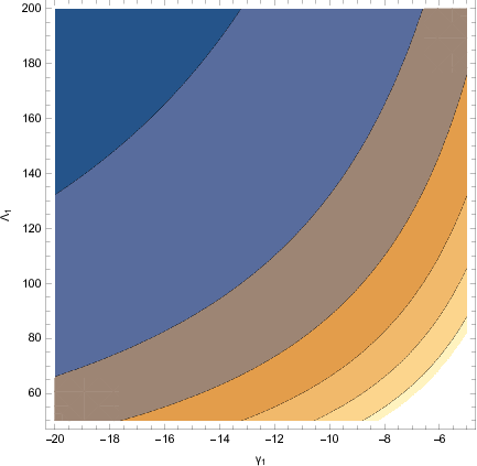
This in turn implies that the scalar field has a unique evolution throughout the inflationary era. Concerning the observational indices, the results are produced by designating the free parameters of the model. Assigning the values (ω\omega, λ1\lambda_{1}, Λ1\Lambda_{1}, V1V_{1}, NN, cc, γ1\gamma_{1})=(1, 1, 100, 1, 60, 0.002, -10) in reduced Planck units where κ=1\kappa=1, then the scalar spectral index of primordial curvature perturbations becomes nS=0.967296n_{S}=0.967296, the tensor spectral index obtains the value nT=−0.0000167n_{T}=-0.0000167 and finally the tensor-to-scalar ratio is equal to r=0.00013223r=0.00013223, which are obviously compatible values with the latest Planck 2018 data. Furthermore, the scalar field seems to decrease with time as ϕi=6.05002\phi_{i}=6.05002 and ϕf=0.0500497\phi_{f}=0.0500497, the sound wave velocity cAc_{A} is equal to unity, as expected hence no ghost instabilities are present. Furthermore, the numerical values of the slow-roll indices are ϵ1=0.00827266\epsilon_{1}=0.00827266, ϵ2=−ϵ1\epsilon_{2}=-\epsilon_{1}, ϵ3=−0.00826439\epsilon_{3}=-0.00826439, ϵ4=−0.00030204\epsilon_{4}=-0.00030204 and finally, indices ϵ5\epsilon_{5} and ϵ6\epsilon_{6} are both equal to ϵ6\epsilon_{6}. The small values of the slow-roll indices is indicative of the validity of the slow-roll approximations imposed previously. In Figs. 1 and 2 we present the dependence of the observational indices on two of the free parameters of the model. As it shown, the viability of the model is achieved for a wide range of the free parameters.

Refer to caption
Refer to caption
Refer to caption
Refer to caption
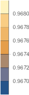
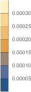
Figure 1: The scalar spectral index of primordial curvature perturbations nSn_{S} (left) and tensor-to-scalar ratio rr (right) as functions of γ1\gamma_{1} and Λ1\Lambda_{1}. Their values are chosen in the ranges [-20,-5] and [50,200] respectively. The plots are derived from the initial assumption where equations (27) through (29) are valid.

There are many differences between the minimally and non-minimally coupled case which are not attributed to this specific choice of coupling functions. Firstly, the string corrections are now indeed inferior compared to other terms and one does not need to decrease λ1\lambda_{1} in order to make this assumption valid. In this case, trivial values seem to yield a viable phenomenology. Moreover, the non-minimally coupled term in stronger than string corrections, as it can easily be inferred from the values of slow-roll indices ϵ3\epsilon_{3}, ϵ5\epsilon_{5} and ϵ6\epsilon_{6}. As a result, indices ϵ5\epsilon_{5} and ϵ6\epsilon_{6} are once again equal, as was the case with the minimally and non-minimally coupled string corrections of the form ξ⁡(ϕ)​𝒢\xi(\phi)\mathcal{G} only. As mentioned before, this specific choice of values for the free parameters leads to the exponent of the scalar potential being equal to 2.001, which is close to 2 as stated before. Hence, the overall model is quite simple as it is comprised of two trivial power law scalar functions and one exponential.

Finally, we mention that each and every approximation made throughout this procedure is indeed valid. Beginning from the slow-roll conditions, which here hinted to be indeed valid from the numerical values of the slow-roll indices during the first horizon crossing, we note that H˙∼𝒪⁡(10)\dot{H}\sim\mathcal{O}(10) whereas H2∼𝒪⁡(103)H^{2}\sim\mathcal{O}(10^{3}), 12​ω​ϕ˙2∼𝒪⁡(10)\frac{1}{2}\omega\dot{\phi}^{2}\sim\mathcal{O}(10) while V∼𝒪⁡(106)V\sim\mathcal{O}(10^{6}) and finally ϕ¨∼𝒪⁡(1)\ddot{\phi}\sim\mathcal{O}(1) compared to H​ϕ˙∼𝒪⁡(100)H\dot{\phi}\sim\mathcal{O}(100). For the string corrections, we mention that 24​ξ˙​H3∼𝒪⁡(10−18)24\dot{\xi}H^{3}\sim\mathcal{O}(10^{-18}) and 9​c​ξ​ϕ˙2​H2∼𝒪⁡(10−23)9c\xi\dot{\phi}^{2}H^{2}\sim\mathcal{O}(10^{-23}) where V∼𝒪⁡(106)V\sim\mathcal{O}(10^{6}), 16​ξ˙​H​H˙∼𝒪⁡(10−21)16\dot{\xi}H\dot{H}\sim\mathcal{O}(10^{-21}), 8​H2​(ξ¨−H​ξ˙)∼𝒪⁡(10−21)8H^{2}(\ddot{\xi}-H\dot{\xi})\sim\mathcal{O}(10^{-21}) and c​ϕ˙​(2​ξ​ϕ˙​(H˙−3​H2)+4​H​ξ​ϕ¨+2​H​ξ˙​ϕ˙)∼𝒪⁡(10−24)c\dot{\phi}\left(2\xi\dot{\phi}(\dot{H}-3H^{2})+4H\xi\ddot{\phi}+2H\dot{\xi}\dot{\phi}\right)\sim\mathcal{O}(10^{-24}) compared to ϕ˙2∼𝒪⁡(10)\dot{\phi}^{2}\sim\mathcal{O}(10) and H​h˙∼𝒪⁡(104)H\dot{h}\sim\mathcal{O}(10^{4}) and finally, ξ′​𝒢∼𝒪⁡(10−17)\xi^{\prime}\mathcal{G}\sim\mathcal{O}(10^{-17}), 3​c​(H2​(ξ˙​H˙+2​ξ​ϕ¨)+2​H​(2​H˙+3​H2)​ξ​ϕ˙)∼𝒪⁡(10−22)3c\left(H^{2}(\dot{\xi}\dot{H}+2\xi\ddot{\phi})+2H(2\dot{H}+3H^{2})\xi\dot{\phi}\right)\sim\mathcal{O}(10^{-22}) in contrast to V′∼𝒪⁡(106)V^{\prime}\sim\mathcal{O}(10^{6}), 6​H2​h′∼𝒪⁡(106)6H^{2}h^{\prime}\sim\mathcal{O}(10^{6}) and 3​ω​H​ϕ˙∼𝒪⁡(103)3\omega H\dot{\phi}\sim\mathcal{O}(10^{3}). Last but not least, for Eq. (8), we mention that neglecting 3​H​h˙3H\dot{h} in order to produce Eq. (27) is valid since V∼𝒪⁡(106)V\sim\mathcal{O}(10^{6}) while 3​H​h˙∼𝒪⁡(104)3H\dot{h}\sim\mathcal{O}(10^{4}). Hence, all the approximations made are indeed valid.

Refer to caption
Refer to caption
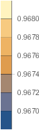
Figure 2: Scalar spectral index of primordial curvature perturbations nSn_{S} depending on parameters γ1\gamma_{1} and Λ1\Lambda_{1} in the value ranges [-20,-5] and [50,200] respectively. In the case of the only change being Eq. (36), the scalar spectral index remains the same. Since the tensor-to-scalar ratio is effectively zero, no corresponding plot is showcased.

As a last comment, it is worth mentioning that different equations of motion are capable of producing similar results. As it was hinted previously, since 3​H​h˙3H\dot{h} is smaller than VV, then using Eq. (8) as Hubble’s form results in the exactly same observational indices, without altering even a single one, thus it is reasonable to discard such term. Moreover, 3​ω​H​ϕ˙3\omega H\dot{\phi} is orders of magnitude smaller than V′V^{\prime} which implies that such term can be omitted. As a matter of fact, doing so leads to an exponent for the scalar potential which is exactly 2. This is the same regardless of keeping 3​H​h˙3H\dot{h} or not in Eq. (8). The most striking result happens when ω​ϕ˙2\omega\dot{\phi}^{2} is neglected from Eq. (6). Assuming that the only change in the equations of motion is,

H˙=2​H2​ξ′4​ξ′′+c​ξ​h′h,\centering\dot{H}=\frac{2H^{2}\xi^{\prime}}{4\xi^{\prime\prime}+c\xi}\frac{h^{\prime}}{h}\,,\@add@centering (36)

then for the same values for the free parameters, the scalar spectral index experiences a mild change as now nS=0.967313n_{S}=0.967313 but on the other hand the tensor spectral index becomes equal to zero, along with the tensor-to-scalar ratio which numerically speaking is r=3⋅10−26r=3\cdot 10^{-26} but essentially is zero. This approach implies that no B (curl) modes are present, which is a striking result compared to the one obtained previously, assuming that the only change is in Hubble rate derivative. The same result is acquired irrespective of 3​H​h˙3H\dot{h} being in Eq. (8) or 3​H​ϕ˙3H\dot{\phi} discarded from Eq. (7). This could be attributed to the choice of the free parameters but many other pairs which were used do not seem to increase the tensor-to-scalar ratio from the value r=10−18r=10^{-18} without breaking the value of the scalar spectral index.

III.2 Exponential Gauss-Bonnet And Power-Law Coupling

Let us now study a similar model but with a different approach. Instead of using a linear Ricci coupling, we shall assume a general power-law model in order to obtain a nonzero h′′h^{\prime\prime} derivative. Suppose that,

ξ⁡(ϕ)=λ2​eγ2​κ​ϕ,\centering\xi(\phi)=\lambda_{2}e^{\gamma_{2}\kappa\phi}\,,\@add@centering (37)
h⁡(ϕ)=Λ2​(κ​ϕ)m,\centering h(\phi)=\Lambda_{2}(\kappa\phi)^{m}\,,\@add@centering (38)

where once again λ2\lambda_{2}, γ2\gamma_{2} and Λ2\Lambda_{2} are the free parameters of the model, but the subscript is changed in order to differentiate from the previous model. Since this choice was made in order to have h′′≠0h^{\prime\prime}\neq 0, we shall take advantage of such feature and see whether a viable phenomenology can be produced. In the following, we shall assume that the proper equations of motion are,

H2=κ2​V3​h,\centering H^{2}=\frac{\kappa^{2}V}{3h}\,,\@add@centering (39)
H˙=−2​H2​ξ′4​ξ′′+c​ξ​(h′′h​4​ξ′4​ξ′′+c​ξ−h′h),\centering\dot{H}=-\frac{2H^{2}\xi^{\prime}}{4\xi^{\prime\prime}+c\xi}\left(\frac{h^{\prime\prime}}{h}\frac{4\xi^{\prime}}{4\xi^{\prime\prime}+c\xi}-\frac{h^{\prime}}{h}\right)\,,\@add@centering (40)
V′+3​H2​(4​ω​ξ′4​ξ′′+c​ξ−2​h′κ2)=0,\centering V^{\prime}+3H^{2}\left(\frac{4\omega\xi^{\prime}}{4\xi^{\prime\prime}+c\xi}-2\frac{h^{\prime}}{\kappa^{2}}\right)=0\,,\@add@centering (41)

where we made certain assumptions and we kept the leading order terms. In the end, we shall make comparisons between the different assumptions which can be made, but for now we shall continue with these. Due to this choice, the scalar potential reads,

V⁡(ϕ)=V2​(κ​ϕ)2​m​e4​γ1​κ2​ω(m−1)​Λ1​((2​γ1​κ)2+c)​(κ​ϕ)1−m,\centering V(\phi)=V_{2}(\kappa\phi)^{2m}e^{\frac{4\gamma_{1}\kappa^{2}\omega}{(m-1)\Lambda_{1}((2\gamma_{1}\kappa)^{2}+c)}(\kappa\phi)^{1-m}}\,,\@add@centering (42)

where now the integration constant is denoted as V2V_{2}. Here, the scalar potential is a combination of a power-law and an exponential function. In particular, the exponential has the form of δ​(κ​ϕ)1−m\delta(\kappa\phi)^{1-m} with δ\delta having a specific form proportional to the rest free parameters. Hence, the potential is a combination of the coupling functions. However, in the case of 3​ω​H​ϕ˙3\omega H\dot{\phi} being inferior to V′V^{\prime} in Eq. (41), the exponential part disappears and the potential is once again a power-law form. The same result is derived in the case we studied in the previous subsection, with a linear Ricci coupling, but now replacing m=1m=1 is forbidden. In addition, the slow-roll indices, or at least the first three, are,

ϵ1=−2​m​γ2​κ​((2​γ2​κ)2+c)​ϕ−4​(m−1)​γ2​κ((2​γ2​κ)2+c)2​ϕ2,\centering\epsilon_{1}=-2m\gamma_{2}\kappa\frac{((2\gamma_{2}\kappa)^{2}+c)\phi-4(m-1)\gamma_{2}\kappa}{((2\gamma_{2}\kappa)^{2}+c)^{2}\phi^{2}}\,,\@add@centering (43)
ϵ2=−ϵ1,\centering\epsilon_{2}=-\epsilon_{1}\,,\@add@centering (44)
ϵ3=2​m​γ2​κ((2​γ2​κ)2+c)​ϕ,\centering\epsilon_{3}=\frac{2m\gamma_{2}\kappa}{((2\gamma_{2}\kappa)^{2}+c)\phi}\,,\@add@centering (45)

Once again, the rest of the slow-roll indices have quite lengthy final form, so we omitted them, however it is worth mentioning that this was not the case with the ξ⁡(ϕ)​𝒢\xi(\phi)\mathcal{G} string corrections for ϵ5\epsilon_{5} and ϵ6\epsilon_{6} at least. Similarly to the previous model, the initial and final value of the scalar field are given by the following expressions,

ϕi=ϕf−4​N​γ2​κ(2​γ2​κ)2+c,\centering\phi_{i}=\phi_{f}-\frac{4N\gamma_{2}\kappa}{(2\gamma_{2}\kappa)^{2}+c}\,,\@add@centering (46)
ϕf=±(−2​c​γ2​κ​m−8​γ23​κ3​m)2−4​(−c2−8​c​γ22​κ2−16​γ24​κ4)​(8​γ22​κ2​m2−8​γ22​κ2​m)−2​c​γ2​κ​m−8​γ23​κ3​m2​(c2+8​c​γ22​κ2+16​γ24​κ4).\centering\phi_{f}=\frac{\pm\sqrt{\left(-2c\gamma_{2}\kappa m-8\gamma_{2}^{3}\kappa^{3}m\right)^{2}-4\left(-c^{2}-8c\gamma_{2}^{2}\kappa^{2}-16\gamma_{2}^{4}\kappa^{4}\right)\left(8\gamma_{2}^{2}\kappa^{2}m^{2}-8\gamma_{2}^{2}\kappa^{2}m\right)}-2c\gamma_{2}\kappa m-8\gamma_{2}^{3}\kappa^{3}m}{2\left(c^{2}+8c\gamma_{2}^{2}\kappa^{2}+16\gamma_{2}^{4}\kappa^{4}\right)}\,.\@add@centering (47)

Since a different equation for Hubble’s derivative is used, we now have two possible forms for the final value of the scalar field, however we shall use only the positive. Letting (ω\omega, λ2\lambda_{2}, Λ2\Lambda_{2}, V2V_{2}, NN, cc, γ2\gamma_{2}, mm)=(1, 1, 100, 1, 60, 0.002, 30, 2) yields viable results since nS=0.965156n_{S}=0.965156, nT=−0.00057706n_{T}=-0.00057706, and r=0.00453744r=0.00453744 which are compatible with the data provided by the Planck 2018 collaboration Akrami:2018odb. Moreover, ϵ1=0.0171237\epsilon_{1}=0.0171237, ϵ3=−0.0168401\epsilon_{3}=-0.0168401 and indices ϵ4\epsilon_{4} through ϵ6\epsilon_{6} are equal to ϵ3\epsilon_{3}.

Refer to caption
Refer to caption
Refer to caption
Refer to caption
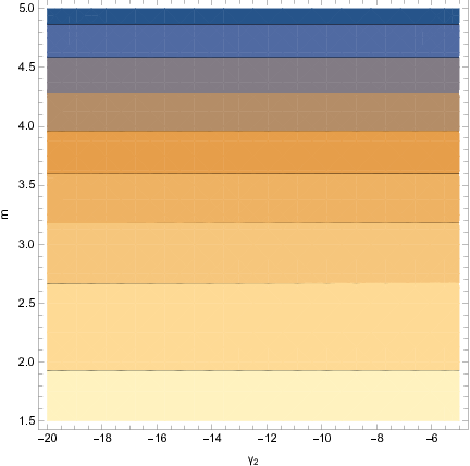
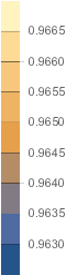
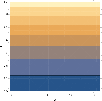
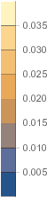
Figure 3: Scalar spectral index of primordial curvature perturbations nSn_{S} (left) and tensor-to-scalar ratio rr (right) depending on parameters γ2\gamma_{2} and mm ranging from [-20,-5] and [1.5,5] respectively. It becomes apparent that the dominant contributor is exponent mm which seems to have different effects on the observed indices. These plots correspond to the initial equations of motion of this particular model.

In this case, the scalar potential has an appealing form. The power-law part is V∼(κ​ϕ)4V\sim(\kappa\phi)^{4} whereas the exponential part is written as V∼e13.3⋅10−4​ϕV\sim e^{\frac{1}{3.3\cdot 10^{-4}\phi}}, implying that the exponential part is not so dominant compared to the power-law. The behavior of the observational indices as functions of several free parameters is depicted in Figs. 3 and 4. As it can be seen, the phenomenological viability of the model is guaranteed for a wide range of the values of the free parameters.

It is worth mentioning that this model is also valid, as all the approximations made indeed apply. Concerning the slow-roll indices, we have H˙∼𝒪⁡(10−4)\dot{H}\sim\mathcal{O}(10^{-4}) whereas H2∼𝒪⁡(10−2)H^{2}\sim\mathcal{O}(10^{-2}), 12​ω​ϕ˙2∼𝒪⁡(10−6)\frac{1}{2}\omega\dot{\phi}^{2}\sim\mathcal{O}(10^{-6}) in contrast to V∼𝒪⁡(10)V\sim\mathcal{O}(10) and lastly, ϕ¨∼𝒪⁡(10−6)\ddot{\phi}\sim\mathcal{O}(10^{-6}) and H​∼˙​𝒪​(10−4)H\dot{\sim}\mathcal{O}(10^{-4}) thus the slow-roll approximations apply. For the string corrections, we have 24​ξ˙​H3∼𝒪⁡(10−33CLOSE24\dot{\xi}H^{3}\sim\mathcal{O}(10^{-33} and 9​c​ξ​ϕ˙2​H2∼𝒪⁡(10−39CLOSE9c\xi\dot{\phi}^{2}H^{2}\sim\mathcal{O}(10^{-39}, 16​ξ˙​H​H˙∼𝒪⁡(10−35)16\dot{\xi}H\dot{H}\sim\mathcal{O}(10^{-35}), 8​H2​(ξ¨−H​ξ˙)∼𝒪⁡(10−35)8H^{2}(\ddot{\xi}-H\dot{\xi})\sim\mathcal{O}(10^{-35}) and c​ϕ˙​(2​ξ​ϕ˙​(H˙−3​H2)+4​H​ξ​ϕ¨+2​H​ξ˙​ϕ˙)∼𝒪⁡(10−39)c\dot{\phi}\left(2\xi\dot{\phi}(\dot{H}-3H^{2})+4H\xi\ddot{\phi}+2H\dot{\xi}\dot{\phi}\right)\sim\mathcal{O}(10^{-39}), ξ′​𝒢∼𝒪⁡(10−31)\xi^{\prime}\mathcal{G}\sim\mathcal{O}(10^{-31}) and 3​c​(H2​(ξ˙​H˙+2​ξ​ϕ¨)+2​H​(2​H˙+3​H2)​ξ​ϕ˙)∼𝒪⁡(10−37)3c\left(H^{2}(\dot{\xi}\dot{H}+2\xi\ddot{\phi})+2H(2\dot{H}+3H^{2})\xi\dot{\phi}\right)\sim\mathcal{O}(10^{-37}) thus string corrections are negligible since in Planck units are effectively zero. Finally, for equations (39) through (41), we mention that 3​H​h˙∼𝒪⁡(10−1)3H\dot{h}\sim\mathcal{O}(10^{-1}) while V∼𝒪⁡(10)V\sim\mathcal{O}(10), ω​ϕ˙2∼𝒪⁡(10−5)\omega\dot{\phi}^{2}\sim\mathcal{O}(10^{-5}) while h′′​ϕ˙2∼𝒪⁡(10−3)h^{\prime\prime}\dot{\phi}^{2}\sim\mathcal{O}(10^{-3}) and H​h˙∼𝒪⁡(10−1)H\dot{h}\sim\mathcal{O}(10^{-1}) hence all the approximations are indeed valid.

Refer to caption
Refer to caption
Refer to caption
Refer to caption
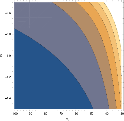
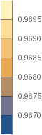
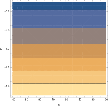
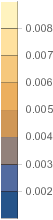
Figure 4: Scalar spectral index of primordial curvature perturbations nSn_{S} (left) and tensor-to-scalar ratio rr (right) as functions of γ2\gamma_{2} and mm which range take values [-100,-35] and [-1.5,-0.5] respectively. These plots correspond to Eq. (8) being the one used. In this case, the scalar spectral index depends on both parameters whereas the tensor-to-scalar ratio keeps being affected only by the power-law exponent mm.

Since V′∼𝒪⁡(10)V^{\prime}\sim\mathcal{O}(10) while 3​ω​H​ϕ˙∼𝒪⁡(10−3)3\omega H\dot{\phi}\sim\mathcal{O}(10^{-3}), the continuity equation can be further simplified. Discarding 3​ω​H​ϕ˙3\omega H\dot{\phi} from Eq. (41) leads to a power-law scalar potential which is similar to the previous model. Also, even if the reader might feel unsatisfied with the numerical value of the slow-roll indices during the first horizon crossing, we mention that by using Eq. (8) as Hubble’s parameter results in a perplexed scalar potential comprised of hypergeometric functions as shown below.

V⁡(ϕ)=V2​(4​m​γ2+(cκ+4​γ22​κ)​ϕ)2​m​e−4γ2κ2ω(−1+2F1(1,1−m,2−m;−((2​γ2​κ)2+c)​ϕ4​m​γ2​κ))(m−1)​Λ2​((2​γ2​κ)2+c),\centering V(\phi)=V_{2}(4m\gamma_{2}+(\frac{c}{\kappa}+4\gamma_{2}^{2}\kappa)\phi)^{2m}e^{-\frac{4\gamma_{2}\kappa^{2}\omega\left(-1+_{2}F_{1}\left(1,1-m,2-m;-\frac{((2\gamma_{2}\kappa)^{2}+c)\phi}{4m\gamma_{2}\kappa}\right)\right)}{(m-1)\Lambda_{2}((2\gamma_{2}\kappa)^{2}+c)}}\,,\@add@centering (48)

In this case, in order to obtain a viable phenomenology, a redefinition of the free parameters is needed. Reassigning the values m=−0.5m=-0.5 and γ2=−60\gamma_{2}=-60 restores compatibility as now nS=0.967962n_{S}=0.967962, r=0.00163923r=0.00163923 and nT=−0.0002041n_{T}=-0.0002041 are acceptable. In this case, the orders of magnitude decrease however the approximations made are still valid, although not in the same ratios. Referring to the slow-roll indices, we now have ϵi∼𝒪⁡(10−3)\epsilon_{i}\sim\mathcal{O}(10^{-3}) for the most part, specifically ϵ1=−0.0040298\epsilon_{1}=-0.0040298, ϵ3=ϵ5=ϵ6=0.00413223\epsilon_{3}=\epsilon_{5}=\epsilon_{6}=0.00413223 and only ϵ4=0.0242458\epsilon_{4}=0.0242458, meaning of order 𝒪⁡(10−2)\mathcal{O}(10^{-2}). The hypergeometric function on the other hand might be bizarre or unappealing, however since 3​ω​H​ϕ˙≪V′3\omega H\dot{\phi}\ll V^{\prime}, one can discard such term from Eq. (41). Consequently, the scalar potential acquires once again a power-law form and the exact same values of free parameters, with the only difference being m=−0.5m=-0.5 and γ2=−60\gamma_{2}=-60, seems to produce the exact same observational indices, as expected.

Similar to the previous subsection, by discarding h′′​ϕ˙2h^{\prime\prime}\dot{\phi}^{2} from Eq. (9), a reasonable assumption as hinted by the order of magnitudes of the showcased previously, then for (ω\omega, λ2\lambda_{2}, Λ2\Lambda_{2}, V2V_{2}, NN, cc, γ2\gamma_{2}, mm)=(1, 1, 100, 1, 60, 0.002, 30, 2), the scalar spectral index is nS=0.966667n_{S}=0.966667, and essentially r=0=nTr=0=n_{T}. In this case as well, no B-modes are expected. The orders of magnitude remain exactly the same, something which is expected since as stated before, h′′​ϕ˙2h^{\prime\prime}\dot{\phi}^{2} is two orders of magnitude lesser than H​h˙H\dot{h}. The same applies to the case of 3​H​h˙3H\dot{h} participating in Eq. (8) and for the scalar potential comprised of hypergeometric function or not and for the values (ω\omega, λ2\lambda_{2}, Λ2\Lambda_{2}, V2V_{2}, NN, cc, γ2\gamma_{2}, mm)=(1, 1, 100, 1, 60, 0.002, -60, -0.5), meaning that B-modes are absent. In both cases for the coupling functions, it seems that the choice for Eq. (6) determines and affects the existence of B-modes. Thus, this feature is a characteristic of the exponential Gauss-Bonnet coupling, since it is the only unchanged function from the previous model.

III.3 Linear Gauss-Bonnet And Power-Law Ricci Coupling

As a final model, we shall study another simple case for the coupling functions, which happens to facilitate our study greatly. Let the Gauss-Bonnet and Ricci scalar non-minimal couplings be chosen as follows,

ξ⁡(ϕ)=λ3​κ​ϕ,\centering\xi(\phi)=\lambda_{3}\kappa\phi\,,\@add@centering (49)
h⁡(ϕ)=Λ3​(κ​ϕ)n,\centering h(\phi)=\Lambda_{3}(\kappa\phi)^{n}\,,\@add@centering (50)

This is an interesting choice for the coupling functions due to the fact that the specific choice for hh simplifies the ratios h′/hh^{\prime}/h and h′′/hh^{\prime\prime}/h which appear in Eq. (6) but also the linear Gauss-Bonnet coupling simplifies ϕ˙\dot{\phi} from Eq. (4) since ξ′′=0\xi^{\prime\prime}=0. The linear Gauss-Bonnet coupling was proved to be inconsistent with the observations in the case of having solely the Gauss-Bonnet term ξ⁡(ϕ)​𝒢\xi(\phi)\mathcal{G} in the Lagrangian, while on the other hand it provided viable results by further assuming the constant-roll assumption for the minimally coupled case h⁡(ϕ)=1h(\phi)=1, hence it is interesting to examine this choice as well. In addition, we shall make use of the following equations of motion,

H2=κ2​V3​h​(1+h′h​4​ξ′4​ξ′′+c​ξ),\centering H^{2}=\frac{\kappa^{2}V}{3h\left(1+\frac{h^{\prime}}{h}\frac{4\xi^{\prime}}{4\xi^{\prime\prime}+c\xi}\right)}\,,\@add@centering (51)
H˙=−2​H2​ξ′4​ξ′′+c​ξ​(h′′h​4​ξ′4​ξ′′+c​ξ−h′h),\centering\dot{H}=-\frac{2H^{2}\xi^{\prime}}{4\xi^{\prime\prime}+c\xi}\left(\frac{h^{\prime\prime}}{h}\frac{4\xi^{\prime}}{4\xi^{\prime\prime}+c\xi}-\frac{h^{\prime}}{h}\right)\,,\@add@centering (52)
V′−6​H2​h′κ2=0,\centering V^{\prime}-6H^{2}\frac{h^{\prime}}{\kappa^{2}}=0\,,\@add@centering (53)

and in the next section we shall overview all the possible approximations that can be performed in order to simplify the equations of motion in the above form.

In the equations of motion, the term ξ′′\xi^{\prime\prime} was kept for the sake of completeness but essentially due to the linear Gauss-Bonnet coupling its zero. For the scalar potential, since the aforementioned equations are used, then subsequently we have,

V⁡(ϕ)=V3​(4​n+c​ϕ2)n,\centering V(\phi)=V_{3}(4n+c\phi^{2})^{n}\,,\@add@centering (54)

In this particular approach, each and every scalar function has a power-law dependence on the scalar field, with the exponents being not necessarily integers , but we shall use only integer values. In addition, the first three slow-roll indices are written as,

ϵ1=−2​n​c​ϕ2−4​n+4(c​ϕ2)2,\centering\epsilon_{1}=-2n\frac{c\phi^{2}-4n+4}{(c\phi^{2})^{2}}\,,\@add@centering (55)
ϵ2=2​c⁡(n−2)​ϕ2−4​n​(n−1)(c​ϕ2)2,\centering\epsilon_{2}=2\frac{c(n-2)\phi^{2}-4n(n-1)}{(c\phi^{2})^{2}}\,,\@add@centering (56)
ϵ3=2​nc​ϕ2.\centering\epsilon_{3}=\frac{2n}{c\phi^{2}}\,.\@add@centering (57)

From ϵ1\epsilon_{1} and Eq. (24), one easily obtains the expressions for the scalar field,

ϕi=c​ϕf2−8​Nc,\centering\phi_{i}=\sqrt{\frac{c\phi_{f}^{2}-8N}{c}}\,,\@add@centering (58)
ϕf=−nc+n⁡(9​n−8)c2,\centering\phi_{f}=\sqrt{-\frac{n}{c}+\sqrt{\frac{n(9n-8)}{c^{2}}}}\,,\@add@centering (59)

For ϕf\phi_{f}, since it is derived from the relation ϵ1=1\epsilon_{1}=1, there exist 4 possible expressions but we shall limit our work only to this particular. In consequence, designating (ω\omega, λ3\lambda_{3}, Λ3\Lambda_{3}, V3V_{3}, NN, cc, nn)=(1, 1, 100, 1, 60, -0.01, 2) then the observational indices take the values nS=0.966395n_{S}=0.966395, nT=−0.0001389n_{T}=-0.0001389 and r=0.0011023r=0.0011023 which are compatible with the latest Planck 2018 data Akrami:2018odb. The model is free of ghost instabilities, since cA=1c_{A}=1 and finally, ϵ1=0.00829\epsilon_{1}=0.00829, ϵ2=−0.000068\epsilon_{2}=-0.000068, ϵ3=−0.00822246\epsilon_{3}=-0.00822246, ϵ4=−0.00822687\epsilon_{4}=-0.00822687, ϵ5=−0.00822249\epsilon_{5}=-0.00822249 and ϵ6=ϵ3\epsilon_{6}=\epsilon_{3} at horizon crossing. These values are indicative of the validity of the slow-roll approximations, but it is worth stating that even though that essentially ϵ5≃ϵ6\epsilon_{5}\simeq\epsilon_{6}, the string corrections seem to have an impact on the dynamics of the model even for trivial values of the free parameters. It is expected that their contribution is not as negligible as previously.

Let us now proceed with the validity of the approximations made throughout the equations of motion. As it was hinted previously, the slow-roll conditions apply as H˙∼𝒪⁡(10−4)\dot{H}\sim\mathcal{O}(10^{-4}) while H2∼𝒪⁡(10−2)H^{2}\sim\mathcal{O}(10^{-2}), 12​ω​ϕ˙2∼𝒪⁡(10−2)\frac{1}{2}\omega\dot{\phi}^{2}\sim\mathcal{O}(10^{-2}) in contrast to V∼𝒪⁡(105)V\sim\mathcal{O}(10^{5}) and finally, ϕ¨∼𝒪⁡(10−6)\ddot{\phi}\sim\mathcal{O}(10^{-6}) whereas H​ϕ˙∼𝒪⁡(10−2)H\dot{\phi}\sim\mathcal{O}(10^{-2}). The string corrections now seem to be enhanced compared to the previous two examples but still inferior. Particularly, 24​ξ˙​H3∼𝒪⁡(10−2)24\dot{\xi}H^{3}\sim\mathcal{O}(10^{-2}), 9​c​ξ​ϕ˙2​H2∼𝒪⁡(10−2)9c\xi\dot{\phi}^{2}H^{2}\sim\mathcal{O}(10^{-2}), 16​ξ˙​H​H˙∼𝒪⁡(10−5)16\dot{\xi}H\dot{H}\sim\mathcal{O}(10^{-5}), 8​H2​(ξ¨−H​ξ˙)∼𝒪⁡(10−3)8H^{2}(\ddot{\xi}-H\dot{\xi})\sim\mathcal{O}(10^{-3}), c​ϕ˙​(2​ξ​ϕ˙​(H˙−3​H2)+4​H​ξ​ϕ¨+2​H​ξ˙​ϕ˙)∼𝒪⁡(10−2)c\dot{\phi}\left(2\xi\dot{\phi}(\dot{H}-3H^{2})+4H\xi\ddot{\phi}+2H\dot{\xi}\dot{\phi}\right)\sim\mathcal{O}(10^{-2}), ξ′​𝒢∼𝒪⁡(10−3)\xi^{\prime}\mathcal{G}\sim\mathcal{O}(10^{-3}) and 3​c​(H2​(ξ˙​H˙+2​ξ​ϕ¨)+2​H​(2​H˙+3​H2)​ξ​ϕ˙)∼𝒪⁡(10−2)3c\left(H^{2}(\dot{\xi}\dot{H}+2\xi\ddot{\phi})+2H(2\dot{H}+3H^{2})\xi\dot{\phi}\right)\sim\mathcal{O}(10^{-2}) which are all negligible compared to the dominant terms as stated before. Finally, we have 3​H​h˙∼𝒪⁡(103)3H\dot{h}\sim\mathcal{O}(10^{3}) and V∼𝒪⁡(105)V\sim\mathcal{O}(10^{5}) thus the first could in principle be neglected, ω​ϕ˙2∼𝒪⁡(10−2)\omega\dot{\phi}^{2}\sim\mathcal{O}(10^{-2}), h′′​ϕ˙2∼𝒪⁡(10)h^{\prime\prime}\dot{\phi}^{2}\sim\mathcal{O}(10) and H​h˙∼𝒪⁡(103)H\dot{h}\sim\mathcal{O}(10^{3}), meaning that once again h′′​ϕ˙2h^{\prime\prime}\dot{\phi}^{2} could be neglected, and finally V′∼𝒪⁡(103)V^{\prime}\sim\mathcal{O}(10^{3}) while 3​ω​H​ϕ˙∼𝒪⁡(10−2)3\omega H\dot{\phi}\sim\mathcal{O}(10^{-2}) thus all the approximations made are indeed valid.

As a final task, it is worth discussing some important issues. Firstly, if one were to keep the term 3​H​ω​ϕ˙3H\omega\dot{\phi} in the continuity equation, as it was the case with the previous two examples, then this would be intrinsically unrealistic, since even though a different scalar potential would be produced, which does not influence the results, for the sake of completeness one would have to add at least the string correction 3​c​(H2​(ξ˙​H˙+2​ξ​ϕ¨)+2​H​(2​H˙+3​H2)​ξ​ϕ˙)3c\left(H^{2}(\dot{\xi}\dot{H}+2\xi\ddot{\phi})+2H(2\dot{H}+3H^{2})\xi\dot{\phi}\right) since it is of the same order, in particular 𝒪⁡(10−2)\mathcal{O}(10^{-2}). Moreover, neglecting 3​H​h˙3H\dot{h} from Eq. (51) and by either increasing by one order Λ3\Lambda_{3} or decreasing λ3\lambda_{3}, produces a viable phenomenology. For instance, Λ3=103\Lambda_{3}=10^{3} gives nS=0.967562n_{S}=0.967562, r=0.00111947r=0.00111947 and nT=−0.00013637n_{T}=-0.00013637 which genuinely speaking are not dramatic changes. The only significant change is ϕ˙\dot{\phi} being independent of ϕ\phi, therefore the evolution of the scalar field follows a linear law ϕ⁡(t)=ϕi+4c​V33​Λ1​t\phi(t)=\phi_{i}+\frac{4}{c}\sqrt{\frac{V_{3}}{3\Lambda_{1}}}t thus the tine instance of the final stage of the inflationary era can be easily extracted. The scalar potential also experiences a mild change since the term 4​n4n in Eq. (54) vanishes. In contrast to the previous cases, neglecting h′′​ϕ˙2h^{\prime\prime}\dot{\phi}^{2} from Eq. (52) does not imply that B-modes are absent. Indeed, both the tensor-to-scalar ratio and the tensor spectral index are quite small as r=3.8⋅10−7r=3.8\cdot 10^{-7} and nT=−1.9⋅10−10n_{T}=-1.9\cdot 10^{-10} but for instance decreasing Λ3\Lambda_{3} to Λ3=6\Lambda_{3}=6 leads to nS=0.968855n_{S}=0.968855 and r=0.000105r=0.000105 which are obviously acceptable values. The same applies to the case of neglecting both h′′​ϕ˙2h^{\prime\prime}\dot{\phi}^{2} and 3​H​h˙3H\dot{h} from equations (52) and (51) respectively.

In consequence, the linear Gauss-Bonnet coupling can work either in the minimally or non-minimally coupled case, under the slow-roll and constant-roll assumption only if extra string corrections are assumed to be present.

IV A Panorama of Different Assumptions and Simplifications that Can be Performed for the Sake of Analyticity

In the previous sections, it was stated that there exist several possible forms that the gravitational equations of motion can take, under different assumptions. In principle none of them is intrinsically unrealistic from the beginning, unless a specific model is incapable of producing phenomenologies compatible with the observational data, after the free parameters of the model are specified. In all the models studied so far, we showcased only some of the possible configurations of the equations of motion due to the fact that there exist multiple paths one can follow for a single model function. Thus, it is worth devoting a section where we present the possible approximated forms of the equations of motion along with the relations that must be satisfied in order for a model to be rendered successful phenomenologically. Before we proceed however, it is worth relabelling the string correction terms in order not to obtain lengthy forms. In particular, we denote string corrections as,

S1​(ϕ)=24​ξ˙​H3−9​c​ξ​H2​ϕ˙2,\centering S_{1}(\phi)=24\dot{\xi}H^{3}-9c\xi H^{2}\dot{\phi}^{2}\,,\@add@centering (60)
S2=−8​H2​(ξ¨−H​ξ˙)−16​ξ˙​H​H˙+2​c​ϕ˙​(ξ⁡(H˙−3​H2)​ϕ˙+2​H​ξ​ϕ¨+H​ξ˙​ϕ˙),\centering S_{2}=-8H^{2}(\ddot{\xi}-H\dot{\xi})-16\dot{\xi}H\dot{H}+2c\dot{\phi}\left(\xi(\dot{H}-3H^{2})\dot{\phi}+2H\xi\ddot{\phi}+H\dot{\xi}\dot{\phi}\right)\,,\@add@centering (61)
S3=ξ′​𝒢−3​c​(H2​(ξ˙​H˙+2​ξ​ϕ¨)+2​H​(2​H˙+3​H2)​ξ​ϕ˙),\centering S_{3}=\xi^{\prime}\mathcal{G}-3c\left(H^{2}(\dot{\xi}\dot{H}+2\xi\ddot{\phi})+2H(2\dot{H}+3H^{2})\xi\dot{\phi}\right)\,,\@add@centering (62)

for convenience. Therefore, the main relations that must be satisfied are the slow-roll conditions,

H˙\displaystyle\centering\dot{H}\@add@centering ≪H2\displaystyle\ll H^{2} 12​ω​ϕ˙2\displaystyle\frac{1}{2}\omega\dot{\phi}^{2} ≪V\displaystyle\ll V ϕ¨\displaystyle\ddot{\phi} ≪H​ϕ˙,\displaystyle\ll H\dot{\phi}\,, (63)

and the string corrections being inferior compared to the rest terms, meaning,

S1\displaystyle\centering S_{1}\@add@centering ≪V\displaystyle\ll V κ2​S2\displaystyle\kappa^{2}S_{2} ≪2​h​H˙\displaystyle\ll 2h\dot{H} S3\displaystyle S_{3} ≪V′.\displaystyle\ll V^{\prime}\,. (64)

The approximations above refer to the order of magnitude and not the sign obviously and are the core assumptions, or in other words the same assumptions as in the minimally coupled case. The equations of motion, even after discarding string corrections SiS_{i} and implementing the slow-roll conditions still contain extra terms and can be further simplified. Genuinely speaking, further assumptions are not mandatory but are quite useful if these are appropriately justified. Let us showcase the necessary relations in case extra assumptions are assumed in each of the equations of motion separately.

We commence from the first equation of motion or in other words Hubble’s form. The possible forms are,

H2=κ2​V3​h​(1+4​ξ′4​ξ′′+c​ξ​h′h),\centering H^{2}=\frac{\kappa^{2}V}{3h\left(1+\frac{4\xi^{\prime}}{4\xi^{\prime\prime}+c\xi}\frac{h^{\prime}}{h}\right)}\,,\@add@centering (65)
H2=κ2​V3​h,\centering H^{2}=\frac{\kappa^{2}V}{3h}\,,\@add@centering (66)
H2=κ2​V3​h′​4​ξ′′+c​ξ4​ξ′.\centering H^{2}=\frac{\kappa^{2}V}{3h^{\prime}}\frac{4\xi^{\prime\prime}+c\xi}{4\xi^{\prime}}\,.\@add@centering (67)

The first two are the ones used mainly in this paper but we mention also the third choice since one can solve easily for squared Hubble’s parameter. Essentially, the first possible form of Eq. (65) has no extra assumptions while the other two have opposite relations which govern the appropriate form. In particular, we have,

h˙\displaystyle\centering\dot{h}\@add@centering ≪H​h\displaystyle\ll Hh H​h\displaystyle Hh ≪h˙,\displaystyle\ll\dot{h}\,, (68)

but since the slow-roll conditions are assumed to hold true, meaning that ϵ3≪1\epsilon_{3}\ll 1 then Eq. (67) is naturally discarded. Thus, there exist only two possible forms, namely equations (65) and (66).

Referring to the scalar field equation, there exist once again two possible forms which one can use. In particular,

V′+3​H2​(4​ω​ξ′4​ξ′′+c​ξ−2​h′κ2)=0,\centering V^{\prime}+3H^{2}\left(\frac{4\omega\xi^{\prime}}{4\xi^{\prime\prime}+c\xi}-2\frac{h^{\prime}}{\kappa^{2}}\right)=0\,,\@add@centering (69)
V′−6​H2​h′κ2=0.\centering V^{\prime}-6H^{2}\frac{h^{\prime}}{\kappa^{2}}=0\,.\@add@centering (70)

The first form is the one used mainly in this framework while the latter was used only in the final example. Genuinely speaking, one is free to also neglect the term 6​H2​h′κ26H^{2}\frac{h^{\prime}}{\kappa^{2}} and thus work with.

V′+ω​H2​12​ξ′4​ξ′′+c​ξ=0,\centering V^{\prime}+\omega H^{2}\frac{12\xi^{\prime}}{4\xi^{\prime\prime}+c\xi}=0\,,\@add@centering (71)

however this case is used for the non-minimally coupled scenario so it was not implemented in the present paper, although it can be used for a weak Ricci coupling without losing integrity of the theory, since in either case the Ricci coupling still participates in Eq. (6). Therefore, in order for the continuity equation to be valid, the following expressions must be valid,

κ2​ϕ˙\displaystyle\centering\kappa^{2}\dot{\phi}\@add@centering ≪2​H​h′\displaystyle\ll 2Hh^{\prime} 2​H​h′\displaystyle 2Hh^{\prime} ≪κ2​ϕ˙,\displaystyle\ll\kappa^{2}\dot{\phi}\,, (72)

for Eq. (70) and Eq. (71) respectively. As expected, the conditions are opposite. Finally, for Hubble’s derivative and in consequence the first slow-roll index, there exist 3!3! possible simplified expressions since 3 terms are present in Eq. (9). Specifically, we have,

H˙=2​H2​ξ′4​ξ′′+c​ξ​h′h,\centering\dot{H}=\frac{2H^{2}\xi^{\prime}}{4\xi^{\prime\prime}+c\xi}\frac{h^{\prime}}{h}\,,\@add@centering (73)
H˙=−H22​(4​ξ′4​ξ′′+c​ξ)2​h′′h,\centering\dot{H}=-\frac{H^{2}}{2}\left(\frac{4\xi^{\prime}}{4\xi^{\prime\prime}+c\xi}\right)^{2}\frac{h^{\prime\prime}}{h}\,,\@add@centering (74)
H˙=−ω​H22​h​(4​κ​ξ′4​ξ′′+c​ξ)2,\centering\dot{H}=-\frac{\omega H^{2}}{2h}\left(\frac{4\kappa\xi^{\prime}}{4\xi^{\prime\prime}+c\xi}\right)^{2}\,,\@add@centering (75)
H˙=2​H2​ξ′4​ξ′′+c​ξ​(h′h−h′′h​4​ξ′4​ξ′′+c​ξ),\centering\dot{H}=\frac{2H^{2}\xi^{\prime}}{4\xi^{\prime\prime}+c\xi}\left(\frac{h^{\prime}}{h}-\frac{h^{\prime\prime}}{h}\frac{4\xi^{\prime}}{4\xi^{\prime\prime}+c\xi}\right)\,,\@add@centering (76)
H˙=2​H2​ξ′4​ξ′′+c​ξ​(h′h−κ2​ωh​4​ξ′4​ξ′′+c​ξ),\centering\dot{H}=\frac{2H^{2}\xi^{\prime}}{4\xi^{\prime\prime}+c\xi}\left(\frac{h^{\prime}}{h}-\frac{\kappa^{2}\omega}{h}\frac{4\xi^{\prime}}{4\xi^{\prime\prime}+c\xi}\right)\,,\@add@centering (77)
H˙=−H22​(4​ξ′4​ξ′′+c​ξ)2​(κ2​ωh+h′′h).\centering\dot{H}=-\frac{H^{2}}{2}\left(\frac{4\xi^{\prime}}{4\xi^{\prime\prime}+c\xi}\right)^{2}\left(\frac{\kappa^{2}\omega}{h}+\frac{h^{\prime\prime}}{h}\right)\,.\@add@centering (78)

Essentially, Eq. (75) is reminiscing of the form of the minimally coupled case, something that can easily be inferred by replacing h⁡(ϕ)=1h(\phi)=1 and this is the reason that we did not study this case in the present paper. On the contrary, it was deemed suitable to examine the contribution of terms proportional to h′h\frac{h^{\prime}}{h} and h′′h\frac{h^{\prime\prime}}{h}. Once again, it is worth mentioning that these are all the possible simplified form of Eq. (9) since the latter is quite difficult to tackle for a given ξ⁡(ϕ)\xi(\phi) and h⁡(ϕ)h(\phi). Hence, the necessary relations that must be satisfied for each separate equation in order for a model to be rendered as viable are,

h′′​4​ξ′4​ξ′′+c​ξ\displaystyle\centering h^{\prime\prime}\frac{4\xi^{\prime}}{4\xi^{\prime\prime}+c\xi}\@add@centering ≪h′\displaystyle\ll h^{\prime} κ2​ω​4​ξ′4​ξ′′+c​ξ\displaystyle\kappa^{2}\omega\frac{4\xi^{\prime}}{4\xi^{\prime\prime}+c\xi} ≪h′,\displaystyle\ll h^{\prime}\,, (79)
κ2​ω\displaystyle\centering\kappa^{2}\omega\@add@centering ≪h′′\displaystyle\ll h^{\prime\prime} h′\displaystyle h^{\prime} ≪h′′​4​ξ′4​ξ′′+c​ξ,\displaystyle\ll h^{\prime\prime}\frac{4\xi^{\prime}}{4\xi^{\prime\prime}+c\xi}\,, (80)
h′′\displaystyle\centering h^{\prime\prime}\@add@centering ≪κ2​ω\displaystyle\ll\kappa^{2}\omega h′\displaystyle h^{\prime} ≪κ2​ω​4​ξ′4​ξ′′+c​ξ,\displaystyle\ll\kappa^{2}\omega\frac{4\xi^{\prime}}{4\xi^{\prime\prime}+c\xi}\,, (81)
κ2​ω\displaystyle\centering\kappa^{2}\omega\@add@centering ≪h′′\displaystyle\ll h^{\prime\prime} κ2​ω​4​ξ′4​ξ′′+c​ξ\displaystyle\kappa^{2}\omega\frac{4\xi^{\prime}}{4\xi^{\prime\prime}+c\xi} ≪h′,\displaystyle\ll h^{\prime}\,, (82)
h′′\displaystyle\centering h^{\prime\prime}\@add@centering ≪κ2​ω\displaystyle\ll\kappa^{2}\omega h′′​4​ξ′4​ξ′′+c​ξ\displaystyle h^{\prime\prime}\frac{4\xi^{\prime}}{4\xi^{\prime\prime}+c\xi} ≪h′,\displaystyle\ll h^{\prime}\,, (83)
h′\displaystyle\centering h^{\prime}\@add@centering ≪κ2​ω​4​ξ′4​ξ′′+c​ξ\displaystyle\ll\kappa^{2}\omega\frac{4\xi^{\prime}}{4\xi^{\prime\prime}+c\xi} h′\displaystyle h^{\prime} ≪h′′​4​ξ′4​ξ′′+c​ξ,\displaystyle\ll h^{\prime\prime}\frac{4\xi^{\prime}}{4\xi^{\prime\prime}+c\xi}\,, (84)

for each H˙\dot{H} respectively. Due to the slow-roll conditions, having h′≪h′′​4​ξ′4​ξ′′+c​ξh^{\prime}\ll h^{\prime\prime}\frac{4\xi^{\prime}}{4\xi^{\prime\prime}+c\xi} is impossible but such possibility is still presented for the sake of completeness. Therefore, there exist essentially 4 viable simplified expressions for H˙\dot{H}. One must be wary of these relations since they produce different phenomenologies, as it was demonstrated previously. Each and every respective relation here must be satisfied and most importantly, the slow-roll conditions along with string corrections being inferior to H2H^{2} and potential terms, in order to obtain a viable phenomenology. Even a single violation results in a false positive model, provided that compatible results where produced. This result is quite similar to the case of pure Einstein-Gauss-Bonnet gravity.

V Conclusions

In this work we developed a theoretical framework that practically revived non-minimally coupled Horndeski theories with non-minimal kinetic coupling. Particularly we studied kinetic coupling corrected non-minimally coupled Einstein-Gauss-Bonnet theory, and we demonstrated how it is possible to have primordial gravitational waves with propagation speed equal to that of light’s. The effective Lagrangian of this model consists of three parts, of a canonical scalar field theory non-minimally coupled to gravity (the Ricci scalar), a non-minimal coupling of the scalar field to the Gauss-Bonnet invariant, and a non-minimal kinetic coupling term. This theory without the Gauss-Bonnet invariant term is excluded by the GW170817 event, but the presence of the Gauss-Bonnet plays a catalytic role in rendering the whole theoretical framework compatible with the GW170817 event. The main constraint we imposed in the theory is the constraint that the propagation speed of the gravitational tensor perturbations is equal to unity in natural units. By also exploiting several slow-roll motivated approximations, we were able to write the initially quite involved equations of motion, in a simple form. Eventually we derived the slow-roll indices of the theory, and the corresponding observations indices. Accordingly, by using several appropriate models, we explicitly demonstrated how the theoretical framework of kinetic coupling corrected non-minimally coupled Einstein-Gauss-Bonnet theory can generate a viable inflationary era, compatible with the Planck 2018 observational data. For each model we showed that the compatibility can be achieved for a wide range of the free parameters of the model. Furthermore, we showed that all the appropriate approximations and assumptions which we made in order to derive the equations of motion in a more analytically tractable form, indeed hold true for all the studied cases, and for the values of the free parameters that guaranteed the viability of each model. The next step in all the classes of the new theoretical framework we developed, is applying the theory in the context of theoretical astrophysics, and specifically aiming for the physics of static neutron stars, basically a direct generalization of Maselli:2016gxk. In the literature, both the scalar Gauss-Bonnet coupling and the scalar field potential are freely chosen, so it is worth investigating the structure and evolution of neutron stars for this class of Horndeski theories we developed, under the constraint that the scalar potential and the non-minimal Gauss-Bonnet coupling are constrained. Also, the presence of the non-minimal kinetic coupling may eventually play an important role, so we aim in the near future to adopt the line of research we just described.

References

  • (1) B. P. Abbott et al. [LIGO Scientific and Virgo], Phys. Rev. Lett. 119 (2017) no.16, 161101 doi:10.1103/PhysRevLett.119.161101 [arXiv:1710.05832 [gr-qc]].
  • (2) B. P. Abbott et al. “Multi-messenger Observations of a Binary Neutron Star Merger,” Astrophys. J. 848 (2017) no.2, L12 doi:10.3847/2041-8213/aa91c9 [arXiv:1710.05833 [astro-ph.HE]].
  • (3) J. M. Ezquiaga and M. Zumalacárregui, Phys. Rev. Lett. 119 (2017) no.25, 251304 doi:10.1103/PhysRevLett.119.251304 [arXiv:1710.05901 [astro-ph.CO]].
  • (4) T. Baker, E. Bellini, P. G. Ferreira, M. Lagos, J. Noller and I. Sawicki, Phys. Rev. Lett. 119 (2017) no.25, 251301 doi:10.1103/PhysRevLett.119.251301 [arXiv:1710.06394 [astro-ph.CO]].
  • (5) P. Creminelli and F. Vernizzi, Phys. Rev. Lett. 119 (2017) no.25, 251302 doi:10.1103/PhysRevLett.119.251302 [arXiv:1710.05877 [astro-ph.CO]].
  • (6) J. Sakstein and B. Jain, Phys. Rev. Lett. 119 (2017) no.25, 251303 doi:10.1103/PhysRevLett.119.251303 [arXiv:1710.05893 [astro-ph.CO]].
  • (7) G. W. Horndeski, Int.J.Theor.Phys. 10, 363 (1974).
  • (8) T. Kobayashi, Rept. Prog. Phys. 82 (2019) no.8, 086901 doi:10.1088/1361-6633/ab2429 [arXiv:1901.07183 [gr-qc]].
  • (9) T. Kobayashi, Phys. Rev. D 94 (2016) no.4, 043511 doi:10.1103/PhysRevD.94.043511 [arXiv:1606.05831 [hep-th]].
  • (10) M. Crisostomi, M. Hull, K. Koyama and G. Tasinato, JCAP 03 (2016), 038 doi:10.1088/1475-7516/2016/03/038 [arXiv:1601.04658 [hep-th]].
  • (11) E. Bellini, A. J. Cuesta, R. Jimenez and L. Verde, JCAP 02 (2016), 053 doi:10.1088/1475-7516/2016/06/E01 [arXiv:1509.07816 [astro-ph.CO]].
  • (12) J. Gleyzes, D. Langlois, F. Piazza and F. Vernizzi, JCAP 02 (2015), 018 doi:10.1088/1475-7516/2015/02/018 [arXiv:1408.1952 [astro-ph.CO]].
  • (13) C. Lin, S. Mukohyama, R. Namba and R. Saitou, JCAP 10 (2014), 071 doi:10.1088/1475-7516/2014/10/071 [arXiv:1408.0670 [hep-th]].
  • (14) C. Deffayet and D. A. Steer, Class. Quant. Grav. 30 (2013), 214006 doi:10.1088/0264-9381/30/21/214006 [arXiv:1307.2450 [hep-th]].
  • (15) D. Bettoni and S. Liberati, Phys. Rev. D 88 (2013), 084020 doi:10.1103/PhysRevD.88.084020 [arXiv:1306.6724 [gr-qc]].
  • (16) K. Koyama, G. Niz and G. Tasinato, Phys. Rev. D 88 (2013), 021502 doi:10.1103/PhysRevD.88.021502 [arXiv:1305.0279 [hep-th]].
  • (17) A. A. Starobinsky, S. V. Sushkov and M. S. Volkov, JCAP 06 (2016), 007 doi:10.1088/1475-7516/2016/06/007 [arXiv:1604.06085 [hep-th]].
  • (18) S. Capozziello, K. F. Dialektopoulos and S. V. Sushkov, Eur. Phys. J. C 78 (2018) no.6, 447 doi:10.1140/epjc/s10052-018-5939-1 [arXiv:1803.01429 [gr-qc]].
  • (19) J. Ben Achour, M. Crisostomi, K. Koyama, D. Langlois, K. Noui and G. Tasinato, JHEP 12 (2016), 100 doi:10.1007/JHEP12(2016)100 [arXiv:1608.08135 [hep-th]].
  • (20) A. A. Starobinsky, S. V. Sushkov and M. S. Volkov, Phys. Rev. D 101 (2020) no.6, 064039 doi:10.1103/PhysRevD.101.064039 [arXiv:1912.12320 [hep-th]].
  • (21) S. V. Sushkov, Phys. Rev. D 80 (2009), 103505 doi:10.1103/PhysRevD.80.103505 [arXiv:0910.0980 [gr-qc]].
  • (22) M. Minamitsuji, Phys. Rev. D 89 (2014), 064017 doi:10.1103/PhysRevD.89.064017 [arXiv:1312.3759 [gr-qc]].
  • (23) E. N. Saridakis and S. V. Sushkov, Phys. Rev. D 81 (2010), 083510 doi:10.1103/PhysRevD.81.083510 [arXiv:1002.3478 [gr-qc]].
  • (24) A. Barreira, B. Li, A. Sanchez, C. M. Baugh and S. Pascoli, Phys. Rev. D 87 (2013), 103511 doi:10.1103/PhysRevD.87.103511 [arXiv:1302.6241 [astro-ph.CO]].
  • (25) S. Sushkov, Phys. Rev. D 85 (2012), 123520 doi:10.1103/PhysRevD.85.123520 [arXiv:1204.6372 [gr-qc]].
  • (26) A. Barreira, B. Li, C. M. Baugh and S. Pascoli, Phys. Rev. D 86 (2012), 124016 doi:10.1103/PhysRevD.86.124016 [arXiv:1208.0600 [astro-ph.CO]].
  • (27) M. A. Skugoreva, S. V. Sushkov and A. V. Toporensky, Phys. Rev. D 88 (2013), 083539 doi:10.1103/PhysRevD.88.083539 [arXiv:1306.5090 [gr-qc]].
  • (28) G. Gubitosi and E. V. Linder, Phys. Lett. B 703 (2011), 113-118 doi:10.1016/j.physletb.2011.07.066 [arXiv:1106.2815 [astro-ph.CO]].
  • (29) J. Matsumoto and S. V. Sushkov, JCAP 11 (2015), 047 doi:10.1088/1475-7516/2015/11/047 [arXiv:1510.03264 [gr-qc]].
  • (30) C. Deffayet, O. Pujolas, I. Sawicki and A. Vikman, JCAP 10 (2010), 026 doi:10.1088/1475-7516/2010/10/026 [arXiv:1008.0048 [hep-th]].
  • (31) L. Granda and W. Cardona, JCAP 07 (2010), 021 doi:10.1088/1475-7516/2010/07/021 [arXiv:1005.2716 [hep-th]].
  • (32) J. Matsumoto and S. V. Sushkov, JCAP 01 (2018), 040 doi:10.1088/1475-7516/2018/01/040 [arXiv:1703.04966 [gr-qc]].
  • (33) C. Gao, JCAP 06 (2010), 023 doi:10.1088/1475-7516/2010/06/023 [arXiv:1002.4035 [gr-qc]].
  • (34) L. Granda, JCAP 07 (2010), 006 doi:10.1088/1475-7516/2010/07/006 [arXiv:0911.3702 [hep-th]].
  • (35) C. Germani and A. Kehagias, Phys. Rev. Lett. 105 (2010), 011302 doi:10.1103/PhysRevLett.105.011302 [arXiv:1003.2635 [hep-ph]].
  • (36) C. Fu, P. Wu and H. Yu, Phys. Rev. D 100 (2019) no.6, 063532 doi:10.1103/PhysRevD.100.063532 [arXiv:1907.05042 [astro-ph.CO]].
  • (37) J. c. Hwang and H. Noh, Phys. Rev. D 71 (2005) 063536 doi:10.1103/PhysRevD.71.063536 [gr-qc/0412126].
  • (38) S. Nojiri, S. D. Odintsov and M. Sami, Phys. Rev. D 74 (2006) 046004 doi:10.1103/PhysRevD.74.046004 [hep-th/0605039].
  • (39) G. Cognola, E. Elizalde, S. Nojiri, S. Odintsov and S. Zerbini, Phys. Rev. D 75 (2007) 086002 doi:10.1103/PhysRevD.75.086002 [hep-th/0611198].
  • (40) S. Nojiri, S. D. Odintsov and M. Sasaki, Phys. Rev. D 71 (2005) 123509 doi:10.1103/PhysRevD.71.123509 [hep-th/0504052].
  • (41) S. Nojiri and S. D. Odintsov, Phys. Lett. B 631 (2005) 1 doi:10.1016/j.physletb.2005.10.010 [hep-th/0508049].
  • (42) M. Satoh, S. Kanno and J. Soda, Phys. Rev. D 77 (2008) 023526 doi:10.1103/PhysRevD.77.023526 [arXiv:0706.3585 [astro-ph]].
  • (43) K. Bamba, A. N. Makarenko, A. N. Myagky and S. D. Odintsov, JCAP 1504 (2015) 001 doi:10.1088/1475-7516/2015/04/001 [arXiv:1411.3852 [hep-th]].
  • (44) Z. Yi, Y. Gong and M. Sabir, Phys. Rev. D 98 (2018) no.8, 083521 doi:10.1103/PhysRevD.98.083521 [arXiv:1804.09116 [gr-qc]].
  • (45) Z. K. Guo and D. J. Schwarz, Phys. Rev. D 80 (2009) 063523 doi:10.1103/PhysRevD.80.063523 [arXiv:0907.0427 [hep-th]].
  • (46) Z. K. Guo and D. J. Schwarz, Phys. Rev. D 81 (2010) 123520 doi:10.1103/PhysRevD.81.123520 [arXiv:1001.1897 [hep-th]].
  • (47) P. X. Jiang, J. W. Hu and Z. K. Guo, Phys. Rev. D 88 (2013) 123508 doi:10.1103/PhysRevD.88.123508 [arXiv:1310.5579 [hep-th]].
  • (48) P. Kanti, R. Gannouji and N. Dadhich, Phys. Rev. D 92 (2015) no.4, 041302 doi:10.1103/PhysRevD.92.041302 [arXiv:1503.01579 [hep-th]].
  • (49) C. van de Bruck, K. Dimopoulos, C. Longden and C. Owen, arXiv:1707.06839 [astro-ph.CO].
  • (50) P. Kanti, J. Rizos and K. Tamvakis, Phys. Rev. D 59 (1999) 083512 doi:10.1103/PhysRevD.59.083512 [gr-qc/9806085].
  • (51) E. O. Pozdeeva, M. R. Gangopadhyay, M. Sami, A. V. Toporensky and S. Y. Vernov, arXiv:2006.08027 [gr-qc].
  • (52) I. Fomin, arXiv:2004.08065 [gr-qc].
  • (53) M. De Laurentis, M. Paolella and S. Capozziello, Phys. Rev. D 91 (2015) no.8, 083531 doi:10.1103/PhysRevD.91.083531 [arXiv:1503.04659 [gr-qc]].
  • (54) S. Chervon, I. Fomin, V. Yurov and A. Yurov, doi:10.1142/11405
  • (55) K. Nozari and N. Rashidi, Phys. Rev. D 95 (2017) no.12, 123518 doi:10.1103/PhysRevD.95.123518 [arXiv:1705.02617 [astro-ph.CO]].
  • (56) S. D. Odintsov and V. K. Oikonomou, Phys. Rev. D 98 (2018) no.4, 044039 doi:10.1103/PhysRevD.98.044039 [arXiv:1808.05045 [gr-qc]].
  • (57) S. Kawai, M. a. Sakagami and J. Soda, Phys. Lett. B 437, 284 (1998) doi:10.1016/S0370-2693(98)00925-3 [gr-qc/9802033].
  • (58) Z. Yi and Y. Gong, Universe 5 (2019) no.9, 200 doi:10.3390/universe5090200 [arXiv:1811.01625 [gr-qc]].
  • (59) C. van de Bruck, K. Dimopoulos and C. Longden, Phys. Rev. D 94 (2016) no.2, 023506 doi:10.1103/PhysRevD.94.023506 [arXiv:1605.06350 [astro-ph.CO]].
  • (60) B. Kleihaus, J. Kunz and P. Kanti, arXiv:1910.02121 [gr-qc].
  • (61) A. Bakopoulos, P. Kanti and N. Pappas, Phys. Rev. D 101 (2020) no.4, 044026 doi:10.1103/PhysRevD.101.044026 [arXiv:1910.14637 [hep-th]].
  • (62) K. i. Maeda, N. Ohta and R. Wakebe, Eur. Phys. J. C 72 (2012) 1949 doi:10.1140/epjc/s10052-012-1949-6 [arXiv:1111.3251 [hep-th]].
  • (63) A. Bakopoulos, P. Kanti and N. Pappas, arXiv:2003.02473 [hep-th].
  • (64) W. Ai, [arXiv:2004.02858 [gr-qc]].
  • (65) S. D. Odintsov and V. K. Oikonomou, Phys. Lett. B 797 (2019) 134874 doi:10.1016/j.physletb.2019.134874 [arXiv:1908.07555 [gr-qc]].
  • (66) V. K. Oikonomou and F. P. Fronimos, [arXiv:2007.11915 [gr-qc]].
  • (67) S. D. Odintsov, V. K. Oikonomou and F. P. Fronimos, Annals Phys. 420 (2020), 168250 doi:10.1016/j.aop.2020.168250 [arXiv:2007.02309 [gr-qc]].
  • (68) V. K. Oikonomou and F. P. Fronimos, [arXiv:2006.05512 [gr-qc]].
  • (69) S. D. Odintsov and V. K. Oikonomou, Phys. Lett. B 805 (2020), 135437 doi:10.1016/j.physletb.2020.135437 [arXiv:2004.00479 [gr-qc]].
  • (70) S. D. Odintsov, V. K. Oikonomou and F. P. Fronimos, [arXiv:2003.13724 [gr-qc]].
  • (71) S. D. Odintsov, V. K. Oikonomou, F. P. Fronimos and S. A. Venikoudis, Phys. Dark Univ. 30 (2020), 100718 doi:10.1016/j.dark.2020.100718 [arXiv:2009.06113 [gr-qc]].
  • (72) R. Easther and K. i. Maeda, Phys. Rev. D 54 (1996) 7252 doi:10.1103/PhysRevD.54.7252 [hep-th/9605173].
  • (73) I. Antoniadis, J. Rizos and K. Tamvakis, Nucl. Phys. B 415 (1994) 497 doi:10.1016/0550-3213(94)90120-1 [hep-th/9305025].
  • (74) I. Antoniadis, C. Bachas, J. R. Ellis and D. V. Nanopoulos, Phys. Lett. B 257 (1991), 278-284 doi:10.1016/0370-2693(91)91893-Z
  • (75) P. Kanti, N. Mavromatos, J. Rizos, K. Tamvakis and E. Winstanley, Phys. Rev. D 54 (1996), 5049-5058 doi:10.1103/PhysRevD.54.5049 [arXiv:hep-th/9511071 [hep-th]].
  • (76) P. Kanti, N. Mavromatos, J. Rizos, K. Tamvakis and E. Winstanley, Phys. Rev. D 57 (1998), 6255-6264 doi:10.1103/PhysRevD.57.6255 [arXiv:hep-th/9703192 [hep-th]].
  • (77) Y. Akrami et al. [Planck Collaboration], arXiv:1807.06211 [astro-ph.CO].
  • (78) A. Maselli, H. O. Silva, M. Minamitsuji and E. Berti, Phys. Rev. D 93 (2016) no.12, 124056 doi:10.1103/PhysRevD.93.124056 [arXiv:1603.04876 [gr-qc]].