Random logic networks: from classical Boolean to quantum dynamics
Abstract
We investigate dynamical properties of a quantum generalization of classical reversible Boolean networks. The state of each node is encoded as a single qubit, and classical Boolean logic operations are supplemented by controlled bit-flip and Hadamard operations. We consider synchronous updating schemes in which each qubit is updated at each step based on stored values of the qubits from the previous step. We investigate the periodic or quasiperiodic behavior of quantum networks, and we analyze the propagation of single site perturbations through the quantum networks with input degree one. A non-classical mechanism for perturbation propagation leads to substantially different evolution of the Hamming distance between the original and perturbed states.
I Introduction
Random Boolean networks exhibit behaviors that lend insights into a variety of fields, serving as generic models describing the dynamics of complex systems ranging from neural Rosin et al. 2013, social Hurford 2001, protein interaction Kauffman et al. 2003, or game theoretic networks Alexander 2003. Studies of random Boolean networks began in earnest with Kauffman’s introduction of a model framework for gene regulatory networks, which consisted of a set of nodes, each having random inputs from nodes chosen at random Kauffman 1969. At each time step, each node is updated according to a randomly assigned Boolean logic operation on its inputs.
The number of possible states of a Boolean network is finite (equal to ). Thus for any initial condition and any deterministic sequence chosen for updating the nodes, the network eventually settles on a periodic attractor. The nature of the set of such attractors for large networks has been a major research topic Flyvbjerg and Kjr 1988; Nielsen and Chuang 2011; Drossel et al. 2005; Derrida and Flyvbjerg 1986; Socolar and Kauffman 2003; Samuelsson and Troein 2003; Greil and Drossel 2005; Drossel et al. 2005; Samuelsson and Socolar 2006; Kaufman and Drossel 2005; Drossel et al. 2005; Paul et al. 2006, with special attention devoted to a dynamical phase transition that occurs as either or the probabilities of assigning different Boolean functions are varied.
The present work is motivated by the possibility of observing a dynamical phase transition or qualitatively different dynamics in random networks of quantum mechanical gates, where the classical states of the nodes are generalized to qubit states and the set of Boolean operations is expanded to include quantum logic functions. Random Boolean networks generally involve high rates of dissipation, as multiple different combinations of the input states to a given node produce the same output state. A naïve introduction of quantum logic into the system retains a high level of dissipation associated with the information loss intrinsic to the projection operations required to create a state of a qubit that is independent of its previous state. Preliminary studies revealed that the introduction of intrinsically quantum mechanical operations leads to a reduction of the dynamics to a single stable fixed point. Removing the projection operators from the quantum system results in reversible dynamics whose classical analogue is found in the reversible Boolean networks introduced by Coppersmith et al. Coppersmith et al. 2001a; Coppersmith et al. 2001b. In contrast to dissipative systems, every state of a reversible Boolean network lies on a periodic orbit; there are no transients. The key questions then concern the distribution of periods (cycle lengths), the scaling of the number of periodic orbits with for different choices or the set of Boolean functions employed, and the stability of cycles under single qubit perturbations.
In the present paper, we consider a modification of reversible random Boolean networks that incorporates inherently quantum operations at some or all of the nodes. We will refer to these as “quantum networks.” A quantum network consists of a set of qubits together with a set of operations determining how each qubit is updated based on the states of a subset of qubits referred to as its inputs. Like classical random Boolean networks, these quantum networks are updated in discrete time steps. Unlike their classical counterparts, however, the state space of the system is not necessarily discrete, as a given qubit can be in an arbitrary superposition of its two basis states (which we take to be the classical Boolean states).
In a quantum network, the operations analogous to Boolean logic functions are unitary operations on the states of some set of qubits. Classical reversible Boolean operations are a subset of these, and a minimal extension of this set includes quantum operations on single qubits. A typical operation might consist, for example, of a classical (reversible) operation applied to several qubits, followed by a quantum operation that creates a superposition of the 0 and 1 states of the output (e.g., a Hadamard operation). To extend the results of Coppermith et al. to the quantum realm, we formulate the reversible dynamics in a way that allows for a natural insertion of quantum operations. Each node in the Coppersmith model is now represented by two qubits, one representing the current state of that node and the other representing its state one time step in the past. This enables an efficient formulation of the dynamics in which the future state of the network depends only on the present state. In a recent study, Franco et al. introduced an equivalent formulation of the class of reversible quantum networks and examined the behavior of networks with Franco et al. 2021.
Our goal is to identify any new effects that arise when unitary operations are included that lead the system out of the discrete classical state space. We focus here on the cycles that arise in small networks and on the divergence of trajectories that differ initially in the state of a single qubit. To study the latter, we extend the concept of classical Hamming distance to one that is well suited to describing a special set of quantum networks employing only Hadamard operations and controlled-not gates. We study the divergence of trajectories in networks in which each qubit receives information from a single other qubit, and describe qualitative differences between the quantum and classical cases.
II Quantum generalizations of reversible Boolean networks
To establish notation, we introduce an example classical reversible Boolean network and describe the formalism for representing it as a quantum circuit. We then describe a particular extension of the set of Boolean truth functions to intrinsically quantum mechanical operations, which will produce the quantum dynamics we are interested in studying.
Consider the reversible classical Boolean networks introduced by Coppersmith et al. Coppersmith et al. 2001a; Coppersmith et al. 2001b. A network consists of spin variables which can be in state or . (Note: We use here rather than to avoid confusion with Pauli matrices below.) The time evolution of each of the Boolean variables depends on the values of other variables. The network updating rule is given by:
| (1) |
where is the value of spin at discrete time step , represents the state vector consisting of the input spins to node at time , and is a Boolean function of inputs. Each node is updated using its own value at time and the output of a truth function . Because can take only the values , this model can be written in the equivalent form
| (2) |
which makes manifest the time-reversal invariance of the dynamics.
A simple example circuit is the , case shown in Fig. 1. It consists of two nodes: is updated according to the OR function ; and is updated according to the AND function . Fig. 1(a) shows the wiring diagram indicating which nodes are inputs to each node, and (b) shows the results of applying Boolean functions and to each possible configuration of input states, i.e. the truth table.

Following Coppersmith et al., we choose to study the case in which the Boolean variables are updated synchronously. To perform the necessary operations, we first introduce one auxiliary bit for each node in the network. This bit holds the updated value of the node until all the operations at a given time step are completed, after which the values of the original bit and the corresponding auxiliary bit are swapped so that the original qubit assumes a new value and the auxiliary qubit holds the value of the original on the previous time step, and the operations for the next time step can begin.
An elementary operation is represented by the diagram in Fig. 1(c), where each line represents one bit, with lines 3 and 4 representing the auxiliary bits corresponding to bits 1 and 2, respectively. (For simplicity, we have relabeled , as , and , as , .) Time proceeds from left to right, and the open and solid dots on lines 1 and 2 indicate that the operation is controlled by the values of those bits. Open and solid dots correspond to states or , respectively. In order for to be applied to , and must take the specified values at time . In this example, just after time will be the result of applying if and only if and . Otherwise, will remain unchanged. The symbols connected by a vertical line indicate the bit values are swapped.
A Boolean function is represented as a sequence of operations, each implementing a single row in the corresponding truth table. We use the symbol to represent an identity operation and to represent a bit-flip (spin-flip). The Boolean logic is represented as shown in Fig. 1(d), where the four operations in the box labeled leave the auxiliary bit unchanged or flip this state, depending upon the value of . The analogous procedure is applied to in the box labeled , depending upon the value of . To complete a single time step, two swap operations are performed, so that and (representing the values at time t) now take the updated values of and , respectively, and and take the values of and on the previous time step.
The classical logic operations can be described as follows, using a notation that generalizes to quantum logic operations. We take each node to be a two-level system (qubit) and work in the computational basis and , where and correspond to and , respectively. The state of an isolated qubit is denoted by . The identity operation, denoted , leaves the state unchanged. The bit-flip operation takes to and to , which is the action induced by the Pauli-X operator, denoted in the diagram by . (In matrix notation, is represented by the Pauli matrix .) If the only operations used in the circuit are (controlled) and (controlled) , each qubit is always in one of the two computational basis states, and the dynamics is equivalent to a classical, reversible Boolean network.
The swap operation also generalizes to quantum systems, as the values of two qubits can be exchanged without loss of information Nielsen and Chuang 2011. We use the symbol to denote a swap, where , e.g., , where stands for .
To introduce nontrivial quantum superpositions and interference effects, we add one additional operation to our set: the Hadamard operation that takes to and to , corresponding to the matrix operation . We note that the Hadamard operation in combination with classical operations can generate entangled states of the network. For example, beginning with a state of two qubits , applying to the first qubit produces the state . If is then applied to the second qubit while controlled by the first, we obtain the entangled state ). As explained below, the restriction of quantum operations to , , and allows us to introduce a measure analogous to the Hamming distance between two network states. We will introduce this measure in Section III.1.
In the computational basis, it is clear that the controlled operations , which each leave all unchanged and change only the auxiliary qubit at node , can be performed in any order within a time step as long as the swap operations are all delayed until the end of the step. Under this protocol, each time step corresponds to a synchronous update of all of the . For each , the swap causes the auxiliary qubit at node at the end of step to takes the value , preparing it to be operated upon in step .
We use the symbol to represent the unitary propagator that advances the entire system through one complete time step. acts on a vector consisting of basis states for the system of nodes, each of which has two associated qubits. Each basis state has the form , where is the state of the auxiliary qubit at node . For the classical operations, the set of all states accessible from a given initial state consists entirely of the finite set of basis states, which immediately implies that the trajectory of the system on repeated application of must be periodic.
Reversibility ensures that each classically accessible state appears in exactly one periodic cycle, and a matrix representation of for a classical network must simply be a permutation matrix with block diagonal form, where each block operates on the subspace of states that form a single cycle. The characteristic polynomial of a single block of dimension is:
| (3) | ||||
| (4) |
which has roots
| (5) |
for integer ranging from to . The eigenvalues of thus consist of the union of complete sets of the roots of unity for a set of values of that sum to . Given the full set of eigenvalues, one can uniquely determine all of the periods by iteratively identifying the largest value of and removing one set of eigenvalues corresponding to it. As an example, Fig. 2 shows the eigenvalues of the classical reversible Boolean network of Fig. 1. Recall that Fig. 1(d) shows 4 qubits, each represented by a horizontal line, that store the values of two qubits for two time steps. Hence there are basis states, and one finds one cycle of length 6, one cycle of length 4 and two cycles of length 3. They correspond to the matrix blocks of dimension , , and (twofold), respectively, associated with the eigenvalues marked by red dots, black crosses, and blue squares, respectively.

When the Hadamard operation is added to the set of logic operations, the distribution of eigenvalues of takes a qualitatively different form; an example is shown in Fig. 3. The Hadamard operation is introduced before the first logic gate on qubit 1 at time t-1 (target-qubit) and is applied on every update step . First, while unitarity ensures that all eigenvalues fall on the unit circle, the eigenvalues are now generally not roots of unity. For networks with 2-input gates, the inclusion of the Hadamard operation makes an infinite set of superposition states accessible Nebe et al. 2001, which can accommodate quasiperiodic trajectories Aharonov 2003 corresponding to eigenvalues with phases that are irrational multiples of . Second, there is no degeneracy in the spectrum in this example.

The situation for networks is qualitatively different. Here, the use of operations consisting only of , , , and ensures that is a member of the Clifford group , defined as follows. Let be a tensor product of Pauli operators . consists of all unitary operators of dimension for which
| (6) |
for every , where represents an overall phase factor of no physical significance. Gottesman 1997. An important property of is that it contains a finite number of elements Ozols 2008; Calderbank et al. 1998. As a result, one can show that for some integer , which implies that all trajectories in these networks are periodic and the eigenvalues are roots of unity.
III Propagation of perturbations
III.1 Distances between states
In this section we introduce a measure for characterizing how perturbations spread through our networks. For classical networks, the evolution of the Hamming distance is often used for this purpose. It is defined as the number of nodes whose values differ between states at the same time step on two different trajectories. Coppersmith et al. Coppersmith et al. 2001b studied evolution of the Hamming distance Wegner 1960 in reversible networks for two states that initially differ at only a single node.
A straightforward generalization of the Hamming distance to quantum states is useful when a state can be written as . We define the distance between and as the number of factors in the first terms in that differ from the identity. This definition reduces to the classical Hamming distance in cases where the elements in include only the identity and the classical bit flips represented by . The restriction to the first terms picks out the factors representing the current states of the qubits, leaving out the auxiliary qubits that represent the state at time .
Given two states related at time by and a set of allowed quantum operations that is restricted to elements of the Clifford group, we have at time :
| (7) | ||||
| (8) | ||||
| (9) | ||||
| (10) |
for some , by Eq. (6). Thus the generalized Hamming distance remains a useful measure of the distance between the future trajectories of the states.
We emphasize again that this extended version of the Hamming distance applies only for networks in which each gate has at most a single input. We also note that any entanglement arising in one trajectory is necessarily mirrored in the other, as the elements of act on single qubits, preserving any entanglement among the different qubits.
III.2 Components of networks
A network drawn from a random ensemble with fixed may contain subsets of nodes forming connected components that have no effective inputs from any other nodes and no outputs to any other nodes. An input to node from node is not effective if the value of is completely independent of .
The numbers and sizes of these independent components strongly depend on the in- and out-degree distributions of the network. The dynamics generated on a given connected component is completely independent of the dynamics of the rest of the network, and it is clear that a perturbation occurring at a single node in a random Boolean network can propagate through only a single connected component. We are therefore interested in the dynamics supported by a single connected component of a network; we leave aside the question of combinatorial effects arising from multiple independent perturbations applied in independent components.
We discuss here only components of networks, where each node has in-degree equal to one, which allows for an analysis of the spread of perturbations using the generalized Hamming distance measure. For dissipative (classical) networks, a connected component must consist of a single loop of nodes with dead-end chains emanating from it (where the loop may be just a single node with a self-input). The dynamics generated by such structures has been characterized in detail Flyvbjerg and Kjr 1988. Here, however, we are interested in reversible networks, which exhibit qualitatively different dynamics from their dissipative counterparts. It is convenient to identify two special cases: (1) a chain, in which the first node receives a constant input and the last has no output (see Fig. 4(a)), and (2) a loop, in which each node receives its input from a neighbor such that the set of input edges forms a closed ring (see Fig. 4(c)). Coppersmith et al. 2001a All more complex components consist of a single loop or a constant node with directed trees emanating from it. The simplest examples are shown in Fig. 4(b) and (d): a chain and a loop with one additional node added.
For reversible networks, the meaning of the specification “” is slightly different because all nodes receive time-delayed self-inputs in addition to inputs from other nodes. here means that each node has exactly one input coming from the value of a node at the current time. Using the implementation in which auxiliary nodes hold the information about time-delayed values, each node effectively receives inputs, one being the auxiliary bit.
We emphasize here that the reversibility of the network dynamics is a logical property, not a guarantee of time-reversal symmetry. The directed links in the network generally break time-reversal symmetry by introducing different mechanisms for propagating information forwards or backwards across any given link.

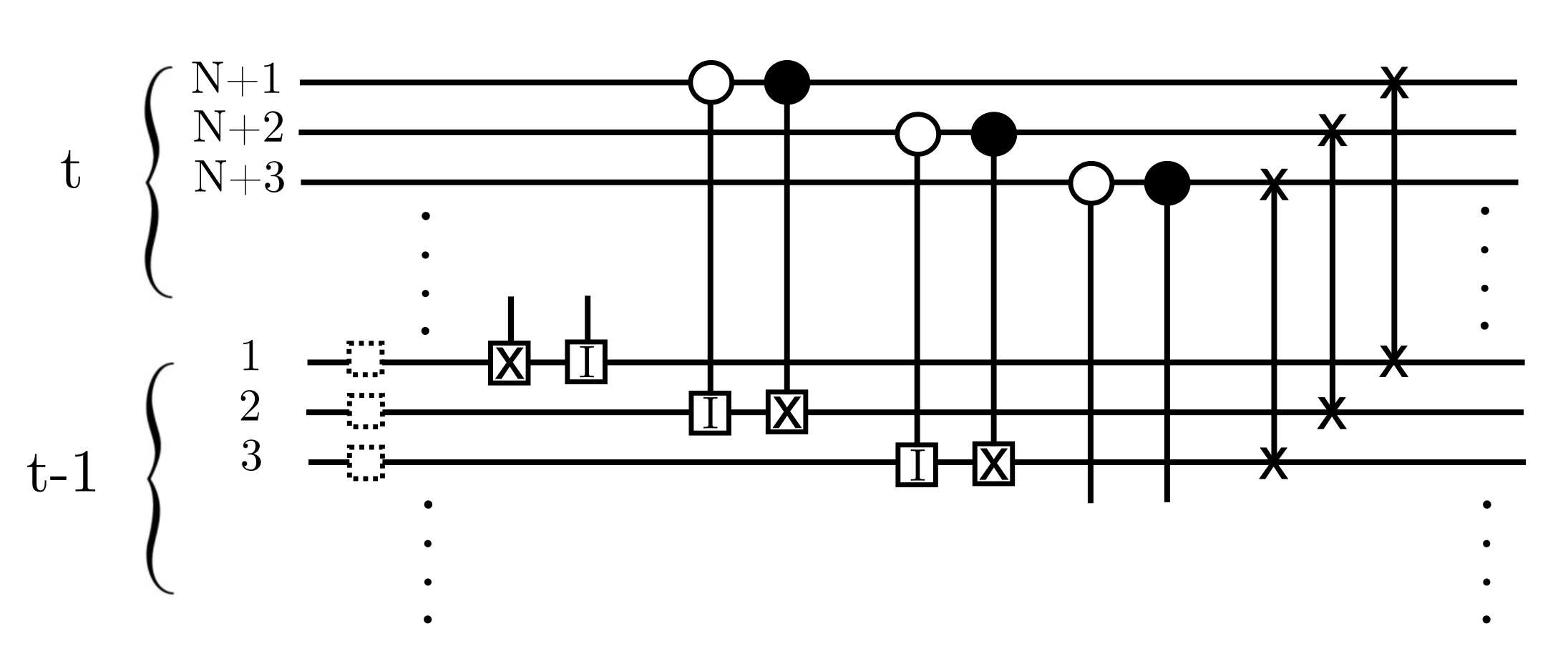
To avoid confusion, we use the term “loop” for a set of nodes connected topologically in a circle, “cycle” for the time-periodic dynamics of a network in state space, and “circuit” to refer to a quantum network.
III.3 Analysis of Spreading Perturbations
In this subsection we analyze the spatial propagation of small perturbations within a single network component. Table 1 shows the transformation of the Pauli matrices under the Hadamard operation. Because our logic operations involve only and , and because the perturbations considered are simple bit flips induced by , the operation relating the perturbed and original trajectories contains only and terms. Fig. 6 shows the classical and quantum mechanical spatial perturbation pattern for a chain (left column) and a loop (right column). Colored squares indicate differences between two trajectories that initially differ by a single bit flip. Blue and orange indicate and factors in .
Coppersmith et al.Coppersmith et al. 2001b already studied the pattern generated by small perturbations in the classical networks. As displayed in Fig. 6(a),(d), the pattern of the classical Hamming distance shows -rotated Sierpinski gaskets Mandelbrot 1977, which are generated by rule 90 of the automata scheme introduced in Wolfram 1983. Using our notation, the Boolean version of rule 90 can be written as
| (11) |
For our observed pattern, the time and space axes are exchanged with respect to the typical depiction of the rule 90 pattern. To show that this pattern results from Eq.(1), Coppersmith et al. consider two trajectories, and , on a chain or loop, where the trajectories begin from initial configurations that differ in one bit; . Next, they define the product of the two solutions as , with . Rewriting Eq. (1) for the case of a chain or loop we obtain
| (12) |
where . The evolution of perturbations can then be expressed as
| (13) |
which mirrors Eq.(11). Note that the evolution of the perturbation is independent of the initial values of the bits and also independent of the functions .
The evolution of a perturbation in the quantum network can be written as follows using the notation defined above. We denote in Eq. (10) by , or, after multiple time steps:
| (14) |
Let and represent the controlled-not gates activated by the control qubit being in state or , respectively. The propagator consists of a sequence of operations that may include or acting on single qubits, or acting on pairs of qubits, and finally a set of (swap) operations. Consider the action of one of these operations on each of the trajectories we are comparing. A given , , or operation clearly has no effect on , as it produces the same effect on both trajectories. One can also confirm by direct enumeration that the effects of and on are the same up to an overall sign that is physically irrelevant; i.e.,
| (15) |
for any and in the set . Thus, as long as the operations are all performed after all of the others, we see that for our networks does not depend on the logic functions associated with the directed links in the network graph. (Note that this is qualitatively similar to that of dissipative loops, where a single bit-flip creates a difference between two trajectories that simply propagates around the loop one step at a time, and the difference between the two is independent of whether a link performs a Copy or a Not operation.)
We now investigate the changes induced when quantum operations are added, considering perturbations applied to an initial state (compare Eq. (1)). From the 2N qubits needed to calculate the evolution of the network, Fig. 6(b),(e) displays qubits 1,…, N for every time step after the application of the Swap operations. In the quantum case, Hadamard operations are applied to each target qubit before applying the logic function. Both types of component, the chain and the loop, exhibit remarkable spatial propagation patterns that are substantially less complex than their classical counterparts. In the following we will discuss the quantum patterns in more detail. They are obtained by calculating Eq. (13) for each operation within the network.
For present purposes, we limit our investigation to networks in which the Hadamard operator is applied at every target qubit once per time step. This subset contains networks that show markedly different properties than the networks realizable by classical operations alone. We refer to the networks with Hadamard operators as “quantum networks” and to those with no Hadamard operators as “classical networks.” Exploration of the behavior of mixed cases in which is applied only to a subset of the qubits is beyond the scope of the present paper.
We begin by studying the evolution of a perturbation on a simple loop. Surprisingly, it spreads in only one direction, as shown in Fig. 6(e). The following pattern emerges:
| (16) | ||||
| (17) | ||||
| (18) | ||||
| (19) | ||||
| (20) | ||||
| (21) |

Each denotes a Pauli matrix, representing a term in the tensor product that relates the trajectory states and . All terms that are not explicitly listed are identity elements. The operations applied to the qubits are denoted by letters on top of the arrows. The presence of two letters on the same arrow indicates that the first operation does not change the state. Superscripts denote the target qubit, and denote the control qubits. The Pauli operators transform under the application of a single-input gate as indicated in Tab. 2. Note that elements are produced by Hadamard operations on single qubits and that elements are produced when the control bits differ by and the targets by .
| Control | Target | |||
Each line in Eqs.(16)-(21) corresponds to a single time step, which is concluded by the (swap) operation. For illustration we discuss in detail the first time step. The Pauli-X operator , describing the difference between the first two target qubits, i.e., at times and , transforms upon the application of a Hadamard operation into a operator which stays in the same position . Next, we apply a non-trivial truth function which is input-dependent. Both possible non-trivial truth functions and yield the same outcome, so need not be further specified. We can use Tab. 2 to show that, since is a perturbation on a target qubit, the application of a truth function generates yet another operator on the -th qubit (), which is a control qubit. Finally, all target and control qubits are swapped (W). Considering Fig. 6(e), we observe that one period of the 12-node loop takes 36 time steps.
We find that, contrary to the classical networks where the perturbations spreads over the whole network component, the quantum system exhibits a localized perturbation which moves through the system affecting only one qubit at a time. We will refer to the configuration of Pauli operators that propagates in this way as a solitary state. Equations. (16)-(21) show how the solitary state moves through the system. The general, 3-time-step, form can be expressed as , where each arrow represents a full time step.
This propagation of a highly localized perturbation in the reversible quantum loop is reminiscent of the situation in classical dissipative networks, where the only structures supporting nontrivial dynamics are loops of COPY and INVERT gates. In the reversible classical loops, a perturbation simply propagates to the next node in the loop on every time step, as the value of a given node is completely determined by the value of its input node on the previous time step. The mechanism sustaining a solitary state in the reversible quantum network, however, relies on quantum coherences between the primary and auxiliary qubits.
Next, we investigate the chain, displayed in Fig. 6(a)-(c). Here a solitary state first propagates in the opposite direction and with a different velocity than the one observed on the loop. Instead of requiring three time steps, the new pattern moves to the next qubit in just one time step. Equations (22)-(27) display the detailed propagation pattern of a chain with an initial perturbation applied at node 1. Each time step is concluded by the application of a swap operation and is indicated with an equation label. In total we display six time steps.
| (22) | ||||
| (23) | ||||
| (24) | ||||
| (25) | ||||
| (26) | ||||
| (27) |
A different solitary state emerges because the first qubit does not have an input. It takes the system five time steps to reach the solitary state, which propagates opposite to the direction of the solitary state produced on the loop. A full propagation step of this state is given in Eq. (27). We see that the Pauli-X operator propagates one bit with every time step. In general this solitary state can be written as: for and with every time step is increased by one.
When this solitary state reaches the end of the chain, it takes the system a few time steps to reach the same solitary state as was seen on the loop, described by Eqs. (18)-(21). The perturbation then reflects again off of the end of the chain, forming a periodic cycle. In total, one period takes approximately time steps (neglecting the transition process between two solitary states).
We note that the Hamming distance for both the chain in Fig. 6(c) and the loop in Fig. 6(f) never exceeds unity in the quantum case, whereas in the classical case the Hamming distance oscillates between zero and five for the case. In general, the maximum Hamming distance is a complicated function of . For , however, we have observed that it is simply the Fibonacci number.
Next, we briefly discuss the perturbation pattern of a slightly more complex network component. We consider the 5-node chain attached to a 1-node loop, displayed in Fig. 7. Two findings should be pointed out in particular. First, if the network component deviates from a plain loop or chain, the perturbation pattern becomes increasingly complex and can strongly differ from the ones shown for loops and chains. We will come back to that point in Section IV.

Second, the nature of the perturbation changes qualitatively as elements appear in . If a controlled gate is applied to the combination of (control) and (target) perturbation, the result is matrices on both the control and target qubit (Tab. 2). In the following we display the equations describing the time steps of the propagation of a perturbation on this network, showing how a Pauli-Y matrix can arise. We consider the case where the perturbation is introduced on the third target qubit (Fig. 7 middle row):
| (28) | ||||
| (29) | ||||
| (30) | ||||
| (31) | ||||
| (32) | ||||
| (33) | ||||
| (34) |
Recall that all figures of perturbation patterns show only the target qubits. Control qubits are not shown, but they are needed to determine the network evolution. For all cases shown, our initial perturbation is a single , with no further perturbation on neither target nor control bits. Adding “invisible” perturbations on the control bits can change the behaviour significantly. For example, considering a simple loop and initializing it with perturbation instead of simply would result in the solitary state described in Eq.(26)-(27), even though the initial perturbation would look the same in our plots.
Considering the fact that in the classical system only matrices are allowed as perturbations, there is only a single mechanism allowing perturbations to spread. If a operator is applied to a control qubit, the controlled gate will create an additional operator on the target qubit as shown in Tab. 2. This leads to the conclusion that for classical structures there is only one direction in which perturbations can spread. This direction is denoted in the network component scheme in the inset of Fig. 7 by black arrows. Only nodes that receive their input directly or indirectly from the initially perturbed node can exhibit perturbations.
The introduction of the Hadamard operation into our system allows for the perturbations to spread in both directions, allowing for a higher Hamming distance to arise in the quantum system. An example is shown in Fig. 7. Each row shows the perturbation pattern for a different initial perturbation. As we can see, the classical network only allows the perturbations to spread alongside the arrows indicating the wiring direction (Fig. 7 top left). The perturbation in the quantum case is confined to the same portion of the network.
While the presence of a branch point in the network gives rise to complicated perturbation patterns in the quantum networks, the implementation of the logic in our qubit systems consists only of linear operations. This means, for example, that a collision between solitary states traveling in opposite directions cannot produce complicated patterns; the two solitary states simply pass through each other. The complexity generated by a branch point is a combinatorial effect associated with the timings of solitary states reflecting off of branch endpoints or traversing a loop to return to the branch point.
IV Magnitude of classical and quantum Hamming distance
In this section, we consider the total Hamming distance and its dependence on network size. Again, only (in-degree 1) networks are considered. We construct ensembles of networks where the input to each node is randomly selected from the full set of nodes. These ensembles thus contain networks consisting of several independent components, and the statistics of perturbation growth are heavily influenced by the statistics of sizes of individual components.
Figure 8 displays the Hamming distance averaged over 1000 random realizations for each network size. It can be seen that the magnitude of the quantum Hamming distance exceeds the classical one but exhibits a similar monotonic increase. As pointed out in previous research Coppersmith et al. 2001b, the total Hamming distance is dependent on the network components of the system. Because initial perturbation (Eq. (10)) is applied to a single qubit, the Hamming distance evolution is determined by the dynamics within that component alone.

Although the quantum Hamming distances of simple chains and loops do not exceed the classical ones, the average quantum Hamming distance is larger because most components contain branch points. It is very rare for a large component to be a simple loop or chain. As we have seen, components with branch points give rise to complicated perturbation patterns with significantly higher Hamming distances than those reached in the classical networks.
V Conclusion
We have presented an approach to constructing quantum circuits that are natural generalizations of reversible random Boolean networks. Our formalism has allowed us to supplement the classical Boolean logic operations with quantum operations. The complexity of the quantum networks depends strongly on their connectivity. While generic systems show quasiperiodic dynamics, a certain nontrivial class of networks of single-input gates shows strictly periodic dynamics. For the special class showing periodic dynamics, we have extended the notion of the Hamming distance between trajectories as a measure to investigate quantitatively the difference patterns generated by small perturbations applied to a network state. For networks where each node has a single input (), these patterns can differ dramatically from their classical counterparts.
We have found that the propagation of perturbations is essentially different in quantum networks. In contrast to classical networks where the perturbations always spread, in the quantum case we find localized solitary perturbations moving through the network step by step. In particular, for simple chains and loops, the perturbation propagates as a localized solitary disturbance at constant velocity.
An open challenge is to develop measures to analyze and interpret the perturbation dynamics generated in quantum networks with multi-input logic gates.
Acknowledgements. We thank Iman Marvian for educational discussions about quantum circuits during the early stages of this work. This work was supported by the Deutsche Forschungsgemeinschaft (DFG, German Research Foundation) - Project Nos. 163436311 - SFB 910, 440145547, and 308748074. LK thanks DAAD for a scholarship and acknowledges the hospitality of Duke University, NC.
References
- Rosin et al. (2013) D. P. Rosin, D. Rontani, D. J. Gauthier, and E. Schöll, Physical review letters 110, 104102 (2013).
- Hurford (2001) R. Hurford, IEEE Transactions on Evolutionary Computation 5, 111 (2001).
- Kauffman et al. (2003) S. Kauffman, C. Peterson, B. Samuelsson, and C. Troein, Proceedings of the National Academy of Sciences 100, 14796 (2003).
- Alexander (2003) J. M. Alexander, Philosophy of Science 70, 1289 (2003).
- Kauffman (1969) S. A. Kauffman, Journal of theoretical biology 22, 437 (1969).
- Flyvbjerg and Kjr (1988) H. Flyvbjerg and N. Kjr, Journal of Physics A: Mathematical and General 21, 1695 (1988).
- Nielsen and Chuang (2011) M. A. Nielsen and I. L. Chuang, Quantum Computation and Quantum Information: 10th Anniversary Edition, 10th ed. (Cambridge University Press, New York, NY, USA, 2011).
- Drossel et al. (2005) B. Drossel, T. Mihaljev, and F. Greil, Physical Review Letters 94, 088701 (2005).
- Derrida and Flyvbjerg (1986) B. Derrida and H. Flyvbjerg, Journal of Physics A: Mathematical and General 19, L1003 (1986).
- Socolar and Kauffman (2003) J. E. Socolar and S. A. Kauffman, Physical review letters 90, 068702 (2003).
- Samuelsson and Troein (2003) B. Samuelsson and C. Troein, Physical Review Letters 90, 098701 (2003).
- Greil and Drossel (2005) F. Greil and B. Drossel, Physical Review Letters 95, 048701 (2005).
- Samuelsson and Socolar (2006) B. Samuelsson and J. E. Socolar, Physical Review E 74, 036113 (2006).
- Kaufman and Drossel (2005) V. Kaufman and B. Drossel, The European Physical Journal B-Condensed Matter and Complex Systems 43, 115 (2005).
- Paul et al. (2006) U. Paul, V. Kaufman, and B. Drossel, Physical Review E 73, 026118 (2006).
- Coppersmith et al. (2001a) S. Coppersmith, L. P. Kadanoff, and Z. Zhang, Physica D: Nonlinear Phenomena 149, 11 (2001a).
- Coppersmith et al. (2001b) S. Coppersmith, L. P. Kadanoff, and Z. Zhang, Physica D: Nonlinear Phenomena 157, 54 (2001b).
- Franco et al. (2021) M. Franco, O. Zapata, D. A. Rosenblueth, and C. Gershenson, Mathematics 9, 792 (2021).
- Nebe et al. (2001) G. Nebe, E. M. Rains, and N. J. Sloane, Designs, Codes and Cryptography 24, 99 (2001).
- Aharonov (2003) D. Aharonov, arXiv preprint quant-ph/0301040 (2003).
- Gottesman (1997) D. Gottesman, Stabilizer codes and quantum error correction, Ph.D. thesis, California Institute of Technology (1997).
- Ozols (2008) M. Ozols, Essays at University of Waterloo, Spring (2008).
- Calderbank et al. (1998) A. R. Calderbank, E. M. Rains, P. Shor, and N. J. Sloane, IEEE Transactions on Information Theory 44, 1369 (1998).
- Wegner (1960) P. Wegner, Commun. ACM 3, 322 (1960).
- Mandelbrot (1977) B. B. Mandelbrot, Fractals: form, chance, and dimension, Vol. 706 (WH Freeman San Francisco, 1977).
- Wolfram (1983) S. Wolfram, Review of Modern Physics 55, 601 (1983).