Bosonic field digitization for quantum computers

Alexandru Macridin, Andy C. Y. Li, Stephen Mrenna, Panagiotis Spentzouris Affiliation: Fermilab, P.O. Box 500, Batavia, Illinois 60510, USA

August 11, 2026

Abstract

Quantum simulation of quantum field theory is a flagship application of quantum computers that promises to deliver capabilities beyond classical computing. The realization of quantum advantage will require methods that can accurately predict error scaling as a function of the resolution and parameters of the model and that can be implemented efficiently on quantum hardware. In this paper, we address the representation of lattice bosonic fields in a discretized field amplitude basis, develop methods to predict error scaling, and present efficient qubit implementation strategies. A low-energy subspace of the bosonic Hilbert space, defined by a boson occupation number cutoff, can be represented with exponentially good accuracy by a low-energy subspace of a finite size Hilbert space. The finite representation construction and the associated errors are directly related to the accuracy of the Nyquist-Shannon sampling and the Finite Fourier transforms of the boson number states in the field and the conjugate-field bases. We analyze the relation between the boson mass, the discretization parameters used for wavefunction sampling and the finite representation size. Numerical simulations of small size $\Phi^{4}$ problems demonstrate that the boson mass optimizing the sampling of the ground state wavefunction is a good approximation to the optimal boson mass yielding the minimum low-energy subspace size. However, we find that accurate sampling of general wavefunctions does not necessarily result in accurate representation. We develop methods for validating and adjusting the discretization parameters to achieve more accurate simulations.

I Introduction

Numerical simulations of systems with continuous variables, whether classical or quantum, require digitization and truncation approximations. For a simulation to be useful, it is essential to know the limit and effect of these approximations. The impact of discretization is especially important when the computational resources required for simulation are scarce. This is a concern for present and near-future quantum computations and classical simulation of complex systems. For example, in the case of strongly correlated systems and lattice field theories, complex schemes are developed Privman 1990; Cardy 2012 to extrapolate the finite size results to the thermodynamic and continuous limits. Unlike the parameters defining the physical problem under investigation, the parameters defining the algorithm (discretization parameters, cutoffs, number of iterations, etc.) should be chosen by the user to optimize the efficiency of the simulations. To do this, criteria are needed to assess whether the choice of these parameters is valid and procedures are needed to adjust them for higher accuracy when necessary. In this paper, we present digitization procedures for bosonic fields, investigate the errors introduced by these procedures and the errors’ dependence on the discretization’s parameters, and introduce a guide for validating and adjusting the discretization’s parameters using feedback from quantum simulations.

Quantum computing offers a change of paradigm for numerical simulations. Many-body and field theory simulations, severely limited on classical computers by the exponentially large memory requirement or the insurmountable Monte Carlo sign problem, might be feasible on future quantum computers. Nevertheless, due to the characteristics of the hardware used for quantum computations, quantum algorithms require a radically different way of storing, manipulating and measuring the information compared to classical computations. As a consequence, specific methods are needed for error analysis, benchmarking and validation.

In a commonly used approach for the numerical simulation of continuous field theories, especially for High Energy Physics problems, the space (or the time-space) coordinates are discretized and the continuous theory is mapped to a lattice field theory. The lattice field problem is solved numerically with the best methods available. The continuous field results are obtained by extrapolating the lattice spacing to zero. This procedure is well studied in the literature and is not the subject of this work. In condensed matter problems, the lattice is given by the physical crystalline structure, and this procedure might not even be necessary. A different approach, which is the focus of this paper, involves the discretization and the truncation of the field amplitude and the representation of the lattice field with qubits.

Systems with bosonic degrees of freedom arise in the Standard Model (Higgs field, gauge fields) and in the low-energy effective models describing collective excitations in condensed matter physics (phonons, magnons, plasmons, etc.). One challenge in developing quantum algorithms for bosonic systems is related to the truncation of the Hilbert space, since, unlike fermion or spin systems, boson systems can have an unbounded occupation number. While it is easy to map a truncated Hilbert space onto the qubit space in a boson number basis, it is difficult to efficiently implement the evolution operator in this basis for many models of interest (such as relativistic scalar field models and electron-phonon systems). For this reason, truncation and discretization in the field amplitude basis has been considered. The first quantum algorithm for scalar field theories using field amplitude discretization was proposed by Jordan et al. Jordan et al. 2012; Jordan et al. 2014. Their error analysis, based on the Chebyshev’s inequality for estimating the probability to have large amplitude fields, implies a number of discretization points per site that scales as ${\cal{O}}(\epsilon^{-1})$ , where $\epsilon$ is the field truncation error. In fact Somma 2016; Macridin et al. 2018a; Macridin et al. 2018b; Klco and Savage 2019, the number of the discretization points scales exponentially better than this, i.e. ${\cal{O}}\left(\log\left(\epsilon^{-1}\right)\right)$ , when the wavefunction is restricted to a low-energy subspace defined by a boson number cutoff. This is a consequence of the properties of the Hermite-Gauss functions Macridin et al. 2018a; Macridin et al. 2018b when using Nyquist-Shannon sampling.

The main focus of this paper is the representation of the lattice bosonic fields on the finite space of the quantum hardware. By representation of a bosonic field on qubits, we mean two things: i) a mapping of the bosonic wavefunctions to qubit wavefunctions and, ii) an isomorphic mapping of the bosonic field operators to discrete field operators acting on the qubit space.

The paper starts with a general overview of the main results and concepts, in Section II.

Section III builds upon the work presented in Refs Macridin et al. 2018a; Macridin et al. 2018b and addresses the construction of the finite representation in the field amplitude basis. It extends the previous work by providing a thorough analysis of the errors associated with this construction and investigating the relation between the sampling errors of the field-variable wavefunction and the boson truncation. By errors in this paper, we mean only the theoretical errors related to the boson field representation on qubits. We do not consider other errors specific to quantum simulations that arise from Trotterization, qubit decoherence, gate fidelity, control noise, etc. The construction of the finite Hilbert space is possible because: i) the boson number wavefunctions both in the field and the conjugate-field bases can be accurately sampled in a finite number of points, which is a consequence of the Nyquist-Shannon sampling theorem applied to almost band-limited and field-limited functions Jaming et al. 2016; Slepian 1976; Landau and Pollak 1962 and, ii) the field and the conjugate field sampling sets can be accurately connected via a finite Fourier transform. The accuracy of the finite representation depends upon the errors arising from sampling, the Finite Fourier transform and the truncation introduced by the boson number cutoff. The dimension of the finite Hilbert space is the same as the number of the sampling points. The low-energy subspace is spanned by the boson number states below a cutoff. For a fixed cutoff, the errors decrease exponentially with increasing number of the sampling points. Empirically, we find that an accuracy $\epsilon\approx 10^{-4}$ requires a finite Hilbert space dimension that is $2$ times larger than the dimension of the low-energy subspace. Many interesting problems, including the broken symmetry phase of the $\Phi^{4}$ field model and the intermediate and the strongly coupled regimes of electron-phonon systems, can be addressed with no more than $6$ qubits per lattice site. However, a word of caution is appropriate. While accurate representation implies accurate sampling, the converse statement is not true. We present examples of functions that can be sampled with great accuracy but have a significant component outside the low-energy subspace. The action of the discrete field operators on states outside the low-energy subspace yields uncontrollable errors. Therefore, a measurement of the boson distribution is necessary to ensure that the wavefunction in a quantum simulation belongs to the low-energy subspace.

The second part of the paper (Section IV) addresses the choice of the discretization parameters in quantum simulations. Different choices of the discretization and sampling intervals correspond to different choices of the boson mass and boson vacuum. The optimal choice of the boson mass corresponds to the minimal boson number cutoff since this choice also implies the minimal size of the finite Hilbert space and implicitly the smallest number of required qubits for implementation. The optimal boson mass is interaction-dependent and it is not known a priori. While finding the optimal boson mass by minimizing the boson number cutoff is impractical, finding the boson mass that maximizes the accuracy of the wavefunction’s sampling is feasible, requiring only local field measurements. By employing exact diagonalization methods for small size $\Phi^{4}$ problems in different parameter regimes, we find that the boson mass providing optimal sampling corresponds to the optimal boson mass.

In the third part of this paper (Section V), we describe measurement methods for the local field and the conjugate-field distributions and additionally for the local boson distribution. We also introduce a practical guide for adjusting and validating the discretization parameters using the feedback from quantum simulation measurements. The guideline follows a simple procedure. First, based on the field distribution measurements, the sampling intervals are adjusted to minimize the sampling errors. The optimal sampling intervals determine the number of discretization points and the boson mass to be used in further simulations, provided that these parameters yield a measured boson distribution below the cutoff. Otherwise, the number of the discretization points is increased. Note that the boson distribution measurement is not needed during the optimization process, but only as a final check after the discretization parameters are adjusted.

In Section VI we discuss the applicability of the discretization method presented here to quantum problems written in the first quantization formalism and the challenges for implementing bosonic algorithms on present and future quantum computers.

Section VII contains our conclusions.

II Overview

The objective of our work is to present a comprehensive study of bosonic field digitization on quantum computers. We present our methodology in great detail to allow the readers to build their own models and perform calculations for specific problems. However, in this section we present a general overview of the main results and concepts.

A general assumption for our method is that the problem of interest can be addressed accurately by restricting the Hilbert space to a finite low-energy subspace defined by a cutoff of maximum $N_{b}$ bosons per lattice site.

While qubit encoding of the boson number states is straightforward (employing, for example, a binary representation of the boson number), the implementation in the boson number basis of the Trotter step operators corresponding to the field dependent interaction terms requires a lengthy decomposition in single and two qubit gates, as discussed in Section III.1. The implementation of these Trotter steps is much simpler in the field amplitude basis, since the Hamiltonian’s field dependent terms are diagonal in this basis. However, representing the truncated low-energy subspace in the field amplitude basis has its challenges, caused mainly by the fact that the field amplitude basis is a continuous and unbounded set. Controlled discretization and truncation procedures are required. We address the construction of the bosonic field representation in the field amplitude basis in Section III.2.

We start constructing the representation of a local Hilbert space in Section III.2.1 and then, in Section III.2.2, the representation for the lattice field is constructed as a direct product of local (one at each lattice site) representations. The construction of the local representation is based on the discretization properties of the Hilbert space’s vectors in the field amplitude basis. In this basis the vectors are equivalent to square integrable functions. Their weight at large argument decreases fast with increasing the argument. The same statement is true for the Fourier transform of these functions. The Nyquist-Shannon sampling theorem can be employed to approximate these functions and, as well, their Fourier transforms. A field variable wavefunction can be reconstructed with ${\cal{O}}(\epsilon)$ accuracy from its value in a finite set of sampled points. Analogous the Fourier transform of the wavefunction can be reconstructed with ${\cal{O}}(\epsilon)$ accuracy from its values in a finite set of conjugated-field sampled points. The set of field sampling points and the set of conjugate-field sampling points are related with ${\cal{O}}(\epsilon)$ accuracy via a Finite Fourier Transform. The error ${\cal{O}}(\epsilon)$ can be decreased by increasing the width of the field and conjugate-field sampling windows. In Sections B.1 and C.2 we calculate upper bounds for the sampling errors, relating these bounds to the wavefunction’s weight outside the field and conjugate-field sampling windows.

To construct the local representation we focus on the sampling properties of boson number states written in the field amplitude basis. Both the boson number states in the field amplitude basis and their Fourier transforms are proportional to Hermite-Gauss functions. For a cutoff $N_{b}$ and an accuracy $\epsilon$ a finite number of discretization points $N_{\varphi}>N_{b}$ can be chosen such that all boson states with $n<N_{b}$ can be sampled with ${\cal{O}}(\epsilon)$ accuracy in $N_{\varphi}$ field-variable points or $N_{\varphi}$ conjugate-field-variable points. The sampling and the recurrence properties of the Hermite-Gauss functions allows us to define a $N_{\varphi}$ finite size Hilbert space $\tilde{\cal{H}}$ and discrete version of the field and conjugate field operators, $\tilde{\Phi}$ and $\tilde{\Pi}$ , acting on $\tilde{\cal{H}}$ . On the subspace of $\tilde{\cal{H}}$ spanned by the first $N_{b}$ eigenvectors of the discrete harmonic oscillator Hamiltonian (i.e. constructed with the discrete field operators, $\tilde{\Phi}$ and $\tilde{\Pi}$ , see Eq. 45) the discrete field operators obey the canonical commutation relation $\left[\tilde{\Phi},\tilde{\Pi}\right]=iI+{\cal{O}}(\epsilon)$ . For a problem of interest, as long as $N_{b}$ is taken large enough such that the contribution of the boson states with $n>N_{b}$ can be neglected, the infinite Hilbert space can be replaced by $\tilde{\cal{H}}$ and the field operators $\Phi$ and $\Pi$ can be replaced by $\tilde{\Phi}$ and $\tilde{\Pi}$ with ${\cal{O}}(\epsilon)$ accuracy. The number of the qubits required for a local representation is $n_{q}=\log\left(N_{\varphi}\right)$ . The representation for a $N$ site lattice field, requires $N\log\left(N_{\varphi}\right)$ qubits.

In practice it is essential to quantify and control the errors. In the last part of Section III.2.1 a numerical analysis of the errors involved in the construction of the finite representation is presented. For $N_{\varphi}=64$ , $N_{\varphi}=128$ and $N_{\varphi}=256$ we calculate the sampling errors and the error associated with the commutations relation of the discrete field operators. These errors are proportional to the tail weights of the boson number states outside sampling interval windows. For a fixed $N_{b}$ the representation error can be reduced exponentially by increasing the number $N_{\varphi}$ of the discretization points. The ratio $N_{b}/N_{\varphi}$ belongs to $[0.3,0.7]$ when the error is in the range $\left[10^{-5},10^{-3}\right]$ . For example, a finite representation with an accuracy of order $10^{-4}$ can be obtained by taking $N_{\varphi}=2N_{b}$ . Encoding this representation requires only one extra qubit (per site) when compared to the encoding in the boson number basis.

The relation between the sampling accuracy of a general wavefunction and its projection onto the low-energy subspace defined by the boson number cutoff is further addressed in Section III.3. While belonging to the low-energy subspace implies accurate sampling (consequence of the representation’s construction described in Section III.2), we find that the converse is not true. We present two examples of functions with small tail weights outside sampling intervals which can be discretized with very good accuracy but have significant weight onto the subspace spanned by boson states with $n>N_{b}$ . As a consequence, the discrete field operators acting on these functions produce uncontrollable errors. Accurate discretization of bosonic field wavefunctions is not enough to ensure the accuracy of the numerical simulations. Boson number distribution measurements are required to ensure the wavefunction belongs to the low-energy subspace.

The construction of the field amplitude representation depends on the definition of bosons, which is not unique. The boson creation and annihilation operators depends on the mass parameter. Different mass bosons are related by a squeezing operator (Bogoliubov transformation). Different choices of the boson mass correspond to different representations. A representation which requires the smallest truncation cutoff $N_{b}$ for a given accuracy is optimal, since it requires the smallest amount of resources for algorithm implementation.

In principle the optimal boson mass can be determined by optimizing the boson distribution as a function of the mass parameter. However, this approach is impractical, since boson distribution measurement is expensive in quantum simulations. On the other hand the measurements of the local field and conjugate-field distribution is straightforward (as discussed in Section V.1). Calculating the sampling windows which minimize the sampling errors of the wavefunction is much easier than optimizing the boson mass for the smallest cutoff $N_{b}$ . In Section IV we investigate the relation between the optimal sampling intervals and the optimal boson mass.

For a given number of the discretization points, the sampling and Finite Fourier Transform errors are the smallest when the weight of the wavefunction outside the field sampling interval $F$ equals the weight of the wavefunction’s Fourier transform outside the conjugate-field sampling interval $K$ . For this choice of the sampling intervals, is the ratio $K/F$ , which equals the representation’s boson mass, the same as the optimal boson mass? While we don’t know the answer in general, numerical simulation for small size lattices find the answer to be yes in many cases. Several examples are presented.

The harmonic oscillator case is illustrated first in Section IV.1. The optimal boson mass is equal to the harmonic oscillator mass parameter $m_{0}$ , since in this case the ground state is the vacuum state. When the boson mass $m_{1}$ is larger (smaller) than $m_{0}$ , for a fixed truncation error, the cutoff number $N_{b}$ increases linearly with increasing the ratio $m_{1}/m_{0}$ ( $m_{0}/m_{1}$ ). The optimal boson mass can be obtained by optimizing the sampling errors. The ratio $K/F=m_{0}$ when $F$ and $K$ are chosen such that the the weight of the wavefunction outside the interval $F$ equals the weight of the wavefunction’s Fourier transform outside the interval $K$ .

Two examples of interacting systems, a local $\phi^{4}$ scalar field (Section IV.2.1) and a two-site $\phi^{4}$ scalar field with imaginary mass (Section IV.2.2) are also presented. In both cases the ground state local field distribution is narrower than the local conjugate-field distribution. Optimal sampling requires the ratio $K/F$ to be larger than the Hamiltonian mass parameter. The ratio $K/F$ determined this way agrees with the optimal boson mass obtained by optimizing the boson number distribution.

In order to enhance the fidelity of applications using our methodology, procedures for validating and adjusting the discretization parameters $N_{\varphi}$ and $m$ for optimal performance, using feedback from quantum simulations, are presented in Section V. The procedures require measurements of the local field distribution, the local conjugate-field distribution and the local boson distribution. These measurements, described in Section V.1, are local, involving the register of $\log(N_{\varphi})$ qubits assigned to encode the bosonic field at one lattice site. The field and conjugate-field distributions require a direct measurement of the qubits. The boson distribution measurement is more laborious. We present two methods for the boson distribution measurement. The first one employs quantum state tomography Altepeter et al. 2004; Nielsen and Chuang 2010 of the local qubit register of size $\log(N_{\varphi})$ . The second method is done by employing Quantum Phase Estimation method Nielsen and Chuang 2010; Cleve et al. 1998 for a local harmonic oscillator and requires an ancillary register of $\log(N_{\varphi})+1$ qubits. The boson distribution can be measured with great accuracy since the energy levels of a harmonic oscillator are equidistant. The probability of having bosons above the cutoff $N_{b}$ is given by the probability to measure integers larger than $N_{b}$ in the ancillary register.

Finally, to support efficient utilization of compute resources, a practical guide for adjusting the discretization parameters in order to improve quantum simulation’s performance is proposed in Section V.2. The initial discretization intervals are determined by assuming a mean-field value for the boson mass. Simulations are run and the local field and conjugate-field distributions are measured. The sampling intervals are adjusted to optimally cover the regions where the field and the conjugate-field distribution have significant support. New simulations which measure the boson distribution are run. If the number of bosons above the cutoff $N_{b}$ is negligible (i.e. it is of the order of the desired accuracy) the discretization parameters are good and the simulation’s results can be trusted. Otherwise the number of the discretization points $N_{\varphi}$ should be increased to accommodate for a larger cutoff $N_{b}$ .

III Low-energy subspace representation

The Hilbert space of a lattice bosonic field is a direct product of local Hilbert spaces at each lattice site. Every local Hilbert space is infinite dimensional, but for most problems can be represented by a finite subspace that contains the relevant degrees of freedom. In general, the relevant degrees of freedom depend on the problem under investigation. In this work, we study the low-energy physics of a field theory where a cut off $N_{b}$ on the boson occupation number can be imposed at each site, such that the states with more than $N_{b}$ bosons per site can be safely neglected. First we briefly discuss the problems associated with the representation of the bosonic field in the boson occupation number basis. Then we address the bosonic field representation in the field amplitude basis.

III.1 Representation in the occupation number basis

The lattice boson number states are a direct product of single site boson number states. At each site the boson number states $|n\rangle$ are eigenstates of the harmonic oscillator Hamiltonian:

\displaystyle H_{h}=\frac{1}{2}\Pi^{2}+\frac{1}{2}m_{0}^{2}\Phi^{2}=m_{0}\left(a^{\dagger}a+\frac{1}{2}\right).

(1)

The creation and the annihilation operators, $a^{\dagger}$ and $a$ , are related to the field operators by

\displaystyle\Phi=\frac{1}{\sqrt{2m_{0}}}\left(a+a^{\dagger}\right)~~\text{and}~~~\Pi=-i\sqrt{\frac{m_{0}}{2}}\left(a-a^{\dagger}\right),

(2)

and $|n\rangle=\frac{1}{\sqrt{n!}}a^{\dagger n}|0\rangle$ , where $|0\rangle$ is the boson vacuum state.

The boson number basis has been used extensively for numerical simulations of bosonic fields on classical computers. For field theories, it is intuitive to define a low-energy subspace by introducing a cutoff $N_{b}$ in the boson number states. The cutoff is chosen such that the states with more than $N_{b}$ bosons have a negligible contribution to the low-energy physics. In general, the cutoff $N_{b}$ depends on the interaction type and strength, but also on the boson mass parameter $m_{0}$ , as can be seen in Eq. 2. A particular choice of the boson mass $m_{0}$ makes the most efficient use of the computational resources, as we will discuss in Section IV.

At each site, boson number states truncated to a cutoff $N_{b}$ can be easily encoded on $n_{q}=\log(N_{b})$ qubits of a quantum computer. For example, a binary representations of the integer number $n$ can be used. Different encodings are also possible Sawaya et al. 2020. However, quantum computation using the boson number representation is difficult to implement in models with field amplitude dependent coupling when the cutoff $N_{b}$ is of the order of $10$ or larger (i.e. when $n_{q}>3$ ). For example, let’s consider coupling terms such as $\sum_{\langle j,l\rangle}\Phi_{j}\Phi_{l}$ present in $\Phi^{4}$ theory or in the phonon models, where $j$ and $l$ are nearest-neighbor lattice site indices. The correspondent Trotter step unitary operator,

\displaystyle e^{-i\theta\Phi_{j}\Phi_{l}}=e^{-i\frac{\theta}{2m_{0}}\left(a_{j}^{\dagger}a_{l}^{\dagger}+a_{j}^{\dagger}a_{l}+a_{j}a_{l}^{\dagger}+a_{j}a_{l}\right)},

(3)

have a dense matrix representation. Since a general unitary of size $k$ requires ${\cal{O}}(4^{k})$ CNOT gates Barenco et al. 1995; Shende et al. 2004; Krol et al. 2021 this Trotter step requires a lengthy decomposition with ${\cal{O}}(4^{2n_{q}})$ two-qubit gates (in this case $k=2n_{q}$ because bosons at two different sites are involved). Similarly, the Trotter step operators for $\frac{\lambda}{4!}\sum_{j}\Phi_{j}^{4}$ interaction in $\Phi^{4}$ theory or for electron-phonon coupling in phonon models requires a decomposition with ${\cal{O}}(4^{n_{q}})$ two-qubit gates (in this case bosons at only one site are involved, hence $k=n_{q}$ ).

For weakly interacting problems with small number of bosonic excitations, quantum algorithms implemented using a boson number representation for the bosonic field might be feasible. The study of different encoding schemes presented in Ref Sawaya et al. 2020 finds that the efficiency of a particular encoding is heavily dependent on the model and on the truncation cutoff. In this study we propose a finite representation suitable for quantum algorithms addressing both weakly and strongly interacting field theories.

III.2 Representation in the field amplitude basis

We consider first the local field construction and then we extend it to lattice field.

III.2.1 Representation of the local Hilbert space

In this section, we address the finite representation of local Hilbert space at a particular lattice site. The local Hilbert space is specified by the field and the conjugate-field operators, $\Phi$ and $\Pi$ , satisfying the canonical commutation relation

\displaystyle\left[\Phi,\Pi\right]=iI.

(4)

The local Hilbert space admits continuous bases, such as the field and the conjugate-field variable ones, and denumerable bases. In the field variable basis, the local Hilbert space is the space of the square integrable functions, $L^{2}(\mathbb{R})$ . The boson number states, discussed in Section III.1, are an example of a denumerable basis.

Considering the difficulties associated with the implementation of Trotter step operators for field amplitude dependent interaction terms in the boson number basis, a more convenient basis for quantum computation is the field amplitude basis $\{|\varphi\rangle\}$ . Here $\{|\varphi\rangle\}$ are the eigenvectors of the field operator, i.e. $\Phi|\varphi\rangle=\varphi|\varphi\rangle$ . The field dependent interaction terms and the corresponding Trotter step operators are diagonal in this basis and easy to implement in a quantum algorithm Macridin et al. 2018b; Macridin et al. 2018a; Li et al. 2021. However, the eigenvectors $\{|\varphi\rangle\}$ are Schwartz distributions and not proper vectors of the Hilbert space. The eigenspectrum of the field operators is continuous and unbounded, but a representation suitable for quantum computation requires discretization and truncation procedures. An apparent difficulty to introducing a finite representation for field operators is caused by their commutation relations. It is known (see for example Ref Gieres 2000) that the canonical commutation relations cannot be satisfied on a finite dimensional space, since on a finite dimensional space the trace of the left hand side of Eq. 4 is zero and the trace of the right hand side is not. However, we construct (see Section III.2.1) a finite Hilbert space $\tilde{{\cal{H}}}$ with a dimension $N_{\varphi}$ larger than the boson number cutoff $N_{b}$ to represent the low-energy subspace of dimension $N_{b}$ . We define the field operators $\tilde{\Phi}$ and $\tilde{\Pi}$ on the finite Hilbert space such that $\left[\tilde{\Phi},\tilde{\Pi}\right]I_{N_{b}}=iI_{N_{b}}$ , where $I_{N_{b}}$ is the projector operator onto the low-energy subspace spanned by the first $N_{b}$ eigenvectors of the harmonic oscillator Hamiltonian. The algebra generated by the operators $\tilde{\Phi}$ and $\tilde{\Pi}$ is isomorphic with the algebra generated by $\Phi$ and $\Pi$ , when both are restricted to the low-energy subspace.

The construction of the finite representation in the field amplitude basis is based on the discrete sampling of the square integrable functions, which is discussed in the next section.

Nyquist-Shannon sampling of wavefunctions

The field amplitude representation of the low-energy subspace is directly related to the discretization and the truncation of wavefunctions belonging to $L^{2}(\mathbb{R})$ space. The discretization procedure takes advantage of the fact that the weight of the square integrable functions at large argument is small and decreases with increasing argument.

To simplify our analysis we consider arbitrary wavefunctions $f(\varphi)\in S(\mathbb{R})$ , where $S(\mathbb{R})$ is the Schwartz space containing the smooth and rapidly decaying functions. The Schwartz space is dense in $L^{2}(\mathbb{R})$ Becnel and Sengupta 2015; Melrose 2017; Suijlekom 2021. The Fourier transform

\displaystyle\hat{f}(\kappa)

\displaystyle=\frac{1}{\sqrt{2\pi}}\int_{-\infty}^{\infty}f(\varphi)e^{-i\kappa\varphi}d\varphi,

(5)

also belongs to $S(\mathbb{R})$ .

We introduce the field limiting projector on the interval $\left[-F,F\right]$

\displaystyle P_{F}=\int_{-F}^{F}|\varphi\rangle\langle\varphi|d\varphi

(6)

and the tail vector

\displaystyle|w_{F}^{f}\rangle

\displaystyle=\left(1-P_{F}\right)|f\rangle\equiv Q_{F}|f\rangle,

(7)

with $|f\rangle=\displaystyle\int f(\varphi)|\varphi\rangle d\varphi$ . The norm of $|w_{F}\rangle$ is equal to the tail weight of $f(\varphi)$ outside the interval $\left[-F,F\right]$ ,

\displaystyle||w_{F}^{f}||=\left(\int_{-\infty}^{-F}|f(\varphi)|^{2}d\varphi+\int_{F}^{\infty}|f(\varphi)|^{2}d\varphi\right)^{\frac{1}{2}}.

(8)

Similarly, we introduce the conjugate-field limiting (we will also call it band-limiting borrowing a signal processing common nomenclature) projector on the interval $\left[-K,K\right]$ ,

\displaystyle P_{K}=\int_{-K}^{K}|\kappa\rangle\langle\kappa|d\kappa

(9)

and the tail vector

\displaystyle|w_{K}^{f}\rangle

\displaystyle=\left(1-P_{K}\right)|f\rangle\equiv Q_{K}|f\rangle.

(10)

The norm of $|w_{K}^{f}\rangle$ is equal to the tail weight of $\hat{f}(\kappa)$ outside the interval $\left[-K,K\right]$ ,

\displaystyle||w_{K}^{f}||=\left(\int_{-\infty}^{-K}|\hat{f}(\kappa)|^{2}d\kappa+\int_{K}^{\infty}|\hat{f}(\kappa)|^{2}d\kappa\right)^{\frac{1}{2}}.

(11)

The tail weight of $f(\varphi)$ outside the interval $\left[-F,F\right]$ can be made as small as desired by increasing $F$ . In the literature Jaming et al. 2016; Slepian 1976; Landau and Pollak 1962, functions with $\epsilon$ small tail weigh are called almost field-limited functions. Analogously, the tail weight of $\hat{f}(\kappa)$ outside the interval $\left[-K,K\right]$ can be made as small as desired by increasing $K$ . The function $f(\varphi)$ is almost band-limited.

When $||w_{K}^{f}||$ is small, the vector $|f\rangle$ can be considered band-limited to a good approximation, i.e. $|f\rangle\approx P_{K}|f\rangle$ . The Nyquist-Shannon sampling theorem Shannon 1949 for band-limited functions can be employed. The following approximation for $f(\varphi)$ (see Appendix A) follows:

\displaystyle f(\varphi)\approx\langle\varphi\vphantom{f}|P_{K}|f\vphantom{\varphi}\rangle=\sum_{i=-\infty}^{\infty}\langle\varphi_{i}\vphantom{f}|P_{K}|f\vphantom{\varphi_{i}}\rangle u_{K}(\varphi-\varphi_{i})\approx\sum_{i=-\infty}^{\infty}f(\varphi_{i})u_{K}(\varphi-\varphi_{i}),

(12)

where

\displaystyle\varphi_{i}=i\Delta_{\varphi},~~~\Delta_{\varphi}=\frac{\pi}{K},~~~\text{and}~~~u_{K}(\varphi)=\text{sinc}\left(\frac{\varphi}{\Delta_{\varphi}}\right)\equiv\frac{\sin\left(\pi\frac{\varphi}{\Delta_{\varphi}}\right)}{\pi\frac{\varphi}{\Delta_{\varphi}}}.

(13)

Moreover, $f(\varphi)$ is small for $|\varphi|>F$ when $F$ is large. The summation in Eq. 12 can be restricted to a finite number $N_{\varphi}$ of points

\displaystyle f(\varphi)\approx\tilde{f}_{\varphi}(\varphi)=\sum_{i=-\frac{N_{\varphi}-1}{2}}^{\frac{N_{\varphi}-1}{2}}f(\varphi_{i})u_{K}(\varphi-\varphi_{i}),

(14)

when the condition $N_{\varphi}\Delta_{\varphi}\geq 2F$ is fulfilled, i.e. when the sampling points cover the window interval $\left[-F,F\right]$ where $f$ has significant support. Note that the Nyquist-Shannon theorem commonly described in the literature considers the summation index $i$ in Eq. 12 to take integer values, but this is easily generalized to half-integer values (see Appendix A), which are more convenient for an even number of discretization points (as required by a qubit representation).

According to Eq. 14, the wavefunction $f(\varphi)$ can be approximated by a finite expansion of sinc functions with the coefficients equal to the value of the function in

\displaystyle N_{\varphi}=\lceil\frac{2}{\pi}FK\rceil

(15)

equidistant points. In Eq. 15 the notation $\lceil x\rceil$ means the ceiling function applied to the real number $x$ , and is equal to the least integer greater than or equal to $x$ . Finding analytical bounds for the accuracy of this approximation is not straightforward, see for example Ref Landau and Pollak 1962. We claim that (see Appendix B.1) a bound for Eq. 14 is:

\displaystyle||f-\tilde{f_{\varphi}}||\lesssim||w_{K}^{f}||+||w_{F}^{f}||+\frac{\pi r_{K}^{f}}{2K}+\sqrt{\frac{\pi}{2K}\left(|f(-F)|^{2}+|f(F)|^{2}\right)}

(16)

where $r_{K}^{f}$ is the weight of $\kappa\hat{f}(\kappa)$ outside the interval $\left[-K,K\right]$ ,

\displaystyle r_{K}^{f}=\bigg(\int_{-\infty}^{-K}\kappa^{2}|\hat{f}(\kappa)|^{2}d\kappa+\int_{K}^{\infty}\kappa^{2}|\hat{f}(\kappa)|^{2}d\kappa\bigg)^{\frac{1}{2}}.

(17)

All terms in Eq. 16 vanish rapidly in the limit of large $F$ and $K$ for the rapidly decaying functions belonging to the Schwartz space.

Using the same reasoning, the conjugate-field variable functions can approximated by a finite expansion of $N_{\varphi}$ sinc functions

\displaystyle\tilde{f}_{\kappa}(\kappa)=\sum_{p=-\frac{N_{\varphi}-1}{2}}^{\frac{N_{\varphi}-1}{2}}\hat{f}(\kappa_{p})u_{F}(\kappa-\kappa_{p}),

(18)

with

\displaystyle\kappa_{p}=p\Delta_{\kappa},~~~\Delta_{\kappa}=\frac{\pi}{F},~~~\text{and}~~~u_{F}(\kappa)=\text{sinc}\left(\frac{\kappa}{\Delta_{\kappa}}\right).

(19)

The vector $|\tilde{f}_{\kappa}\rangle$ differs from $|f\rangle$ by

\displaystyle||f-\tilde{f}_{\kappa}||\lesssim||w_{K}^{f}||+||w_{F}^{f}||+\frac{\pi r_{F}^{f}}{2F}+\sqrt{\frac{\pi}{2F}\left(|\hat{f}(-K)|^{2}+|\hat{f}(K)|^{2}\right)}

(20)

where $r_{F}^{f}$ is the weight of $\varphi f(\varphi)$ outside the interval $\left[-F,F\right]$ ,

\displaystyle r_{F}^{f}=\bigg(\int_{-\infty}^{-F}\varphi^{2}|f(\varphi)|^{2}d\varphi+\int_{F}^{\infty}\varphi^{2}|f(\varphi)|^{2}d\varphi\bigg)^{\frac{1}{2}}.

(21)

The accuracy of both approximations of $|f\rangle$ , $|\tilde{f}_{\varphi}\rangle$ and $|\tilde{f}_{\kappa}\rangle$ are determined by the values of $f(\varphi)$ and $\hat{f}(\kappa)$ outside the intervals $\left[-F,F\right]$ and $\left[-K,K\right]$ , respectively. Note that $|\tilde{f}_{\varphi}\rangle$ is a band-limited function and $|\tilde{f}_{\kappa}\rangle$ is a field-limited function, while $|f\rangle$ isn’t necessary band-limited or field-limited. An approximation of $|f\rangle$ that is both band-limited and field-limited does not exist, since no analytical function, except the zero function, can be simultaneously band-limited and field-limited Landau and Pollak 1962; Slepian 1976; Engelberg 2008.

The vector $|f\rangle$ can be reconstructed from a set containing the field sampled values $\{f(\varphi_{i})\}_{i}$ or from a set containing the conjugate-field sampled values $\{\hat{f}(\kappa_{p})\}_{p}$ . The accuracy of the reconstruction is determined by the values of $|f\rangle$ outside the field and conjugate-field sampling intervals. However, accurate sampling is only a necessary condition for the representation of the bosonic field on quantum hardware. A quantum algorithm also requires implementation of unitary operators that can describe accurately the evolution of the system. While the field and conjugate-field functions $f(\varphi)$ and $\hat{f}(\kappa)$ are related by a continuous Fourier transform, the representation for bosonic fields on qubits is based on the assumption that a Finite Fourier Transform (FFT) connects the sampling sets $\{f(\varphi_{i})\}_{i}$ and $\{\hat{f}(\kappa_{p})\}_{p}$ with high precision, as will be discussed in Section III.2.1.

The difference between the FFT $\tilde{\cal{F}}$ of the field sampling set $\{f(\varphi_{i})\}_{i}$ denoted by $\{(\tilde{\cal{F}}f)(\kappa_{p})\}_{p}$ and the function’s Fourier transform in the conjugate-field sampling points $\{\hat{f}(\kappa_{p})\}_{p}$ is determined by the weight of the function outside the sampling windows and decreases with increasing $F$ and $K$ . In Section C.1 we find that

\displaystyle\Delta_{\kappa}\sum_{p=-\frac{N_{\varphi}-1}{2}}^{\frac{N_{\varphi}-1}{2}}|(\tilde{\cal{F}}f)(\kappa_{p})-\hat{f}(\kappa_{p})|^{2}

\displaystyle\lesssim 2\left(||w_{F}^{f}||^{2}+||w_{K}^{f}||^{2}\right)+\frac{\pi}{K}\left(|f(-F)|^{2}+|f(F)|^{2}\right)+\frac{\pi}{F}\left(|\hat{f}(-K)|^{2}+|\hat{f}(K)|^{2}\right).

(22)

Similarly, the difference between the inverse finite Fourier transform of the set $\{\hat{f}(\kappa_{p})\}_{p}$ , denoted by $\{(\tilde{\cal{F}}^{-1}\hat{f})(\varphi_{i})\}_{i}$ , and the function at the field sampling points, $\{f(\varphi_{i})\}_{i}$ , is given by

\displaystyle\Delta_{\varphi}\sum_{i=-\frac{N_{\varphi}-1}{2}}^{\frac{N_{\varphi}-1}{2}}|(\tilde{\cal{F}}^{-1}f)(\varphi_{i})-f(\varphi_{i})|^{2}

\displaystyle\lesssim 2\left(||w_{F}^{f}||^{2}+||w_{K}^{f}||^{2}\right)+\frac{\pi}{K}\left(|f(-F)|^{2}+|f(F)|^{2}\right)+\frac{\pi}{F}\left(|\hat{f}(-K)|^{2}+|\hat{f}(K)|^{2}\right).

(23)

The definition of $\tilde{\cal{F}}$ and $\tilde{\cal{F}}^{-1}$ is given by Eqs. 188 and 189 in Section C.1.

Finite representation construction

In this section, we define the discrete field operators and construct the finite Hilbert space of the representation based on the discretization properties of the boson number states. This section ends with a detailed analysis of the errors generated by the approximations used in this construction.

Sampling of Hermite-Gauss functions.

The wavefunctions’ sampling procedures discussed in the previous section are applied here to the boson number states in the field amplitude basis. The boson number states form a denumerable basis for the local Hilbert space and provide an intuitive way to introduce the relevant low-energy subspace for the problem under investigation.

In the field amplitude basis the boson number state $|n\rangle$ is the Hermite-Gauss (HG) function of order $n$ ,

\displaystyle\langle\varphi\vphantom{n}|n\vphantom{\varphi}\rangle\equiv\phi_{n}(\varphi)=\left(\frac{m_{0}}{\pi}\right)^{1/4}\frac{1}{\sqrt{2^{n}n!}}e^{-\frac{m_{0}\varphi^{2}}{2}}H_{n}(\sqrt{m_{0}}\varphi),

(24)

where $H_{n}$ is the Hermite polynomial of order $n$ . The Fourier transform of $\phi_{n}(\varphi)$ to the conjugate-field variable $\kappa$ is also proportional to a Hermite-Gauss function of order $n$ Gradshteyn and Ryzhik 1980,

\displaystyle\langle\kappa\vphantom{n}|n\vphantom{\kappa}\rangle\equiv\hat{\phi}_{n}(\kappa)=\frac{\left(-i\right)^{n}}{\pi^{1/4}m_{0}^{1/4}\sqrt{2^{n}n!}}e^{-\frac{\kappa^{2}}{2m_{0}}}H_{n}(\frac{\kappa}{\sqrt{m_{0}}}).

(25)

The recurrence properties of the HG functions (see also Eq. 2) imply

	$\displaystyle\varphi\phi_{n}(\varphi)$	$\displaystyle=\langle\varphi\vphantom{n}\|\Phi\|n\vphantom{\varphi}\rangle=\frac{1}{\sqrt{2m_{0}}}\left(\sqrt{n}\phi_{n-1}(\varphi)+\sqrt{n+1}\phi_{n+1}(\varphi)\right)$		(26)
	$\displaystyle\kappa\hat{\phi}_{n}(\kappa)$	$\displaystyle=\langle\kappa\vphantom{n}\|\Pi\|n\vphantom{\kappa}\rangle=-i\sqrt{\frac{m_{0}}{2}}\left(\sqrt{n}\hat{\phi}_{n-1}(\kappa)-\sqrt{n+1}\hat{\phi}_{n+1}(\kappa)\right).$		(27)

Refer to caption — Figure 1: a) Hermite-Gauss functions $\phi_{0}(\varphi)$ , $\phi_{15}(\varphi)$ , and $\phi_{34}(\varphi)$ (solid, dashed and, respectively, dot-dashed lines) and the discrete harmonic oscillator (with $m_{0}=1$ ) eigenstates $\tilde{\phi}_{0}(\varphi_{i})$ , $\tilde{\phi}_{15}(\varphi_{i})$ , and $\tilde{\phi}_{34}(\varphi_{i})$ (circle, square and, respectively, triangle symbols) for a finite Hilbert space with $N_{\varphi}=64$ discretization points. Within ${\cal{O}}(10^{-4})$ accuracy the support of the HG functions with $n\leq N_{b}=34$ is inside the interval $\left[-L,L\right]$ , where $L=\sqrt{\pi N_{\varphi}/2}$ (see Eq. 29). These HG functions are sampled accurately by the discrete harmonic oscillator eigenvectors. b) The support of $\phi_{57}(\varphi)$ (solid line) has significant weight outside $\left[-L,L\right]$ and the function cannot be sampled by the eigenvector $\tilde{\phi}_{57}(\varphi_{i})$ (circle symbols) of the discrete harmonic oscillator.

The HG functions have significant weight on an interval centered on zero and are exponentially small at large argument, as can be inferred from Eqs. 24 and 25. The width of the window needed to contain a significant weight increases with increasing order $n$ . Several HG functions are shown in Fig. 1 for illustration.

For a boson state $\phi_{n}(\varphi)$ , the sampling errors appearing in Eqs. 16, 20, 22 and 23 can be written in terms of the tail weights $||w^{\phi_{n}}_{F}||$ and $||w^{\phi_{n}}_{K}||$ . This can be understood by noting that $||w^{\phi_{n}}_{F}||$ and $||w^{\phi_{n}}_{K}||$ are monotonically decreasing with increasing $F$ , respectively $K$ , when $F$ and $K$ are large enough. Therefore the dependence $F=F(||w^{\phi_{n}}_{F}||)$ , and $K=K(||w^{\phi_{n}}_{K}||)$ can be found, i.e. the sampling interval widths can be expressed as function of the tail weights. As a consequence, all of the terms $r^{\phi_{n}}_{F}$ , $r^{\phi_{n}}_{K}$ , $|\phi_{n}(F)|^{2}$ and $|\hat{\phi}_{n}(K)|^{2}$ can be written in terms of the tail weights.

For HG functions, a parameter $L$ can be defined that relates the field and conjugate-field sampling windows when $||w^{\phi_{n}}_{F}||=||w^{\phi_{n}}_{K}||$ :

\displaystyle F=\frac{L}{\sqrt{m_{0}}}\text{, }~~~K=L\sqrt{m_{0}}.

(28)

The HG function $\phi_{n}(\varphi)$ and its Fourier transform $\hat{\phi}_{n}(\kappa)$ , can be sampled with a finite set of points

\displaystyle N_{\varphi}=\lceil\frac{2}{\pi}FK\rceil=\lceil\frac{2}{\pi}L^{2}\rceil,

(29)

and an error determined by the function tail weights,

\displaystyle\epsilon_{w}(n,L)\equiv||w^{\phi_{n}}_{F}||=||w^{\phi_{n}}_{K}||.

(30)

By considering only the leading term $2^{n}\varphi^{n}$ of the Hermite polynomial $H_{n}(\varphi)$ , employing partial integration, and applying Stirling’s formula, it can be shown that

\displaystyle\epsilon_{w}^{2}(n,L)\lesssim\frac{1}{L\sqrt{\pi}}\frac{2^{n}L^{2n}}{n!}e^{-L^{2}}\approx e^{-L^{2}-\ln\sqrt{2}L\pi}e^{n\ln\frac{2eL^{2}}{n}}e^{-\frac{1}{2}\ln n}.

(31)

For a fixed $n$ , the tail weight $\epsilon_{w}(n,L)$ decreases exponentially with increasing $L$ . For a fixed $L$ and $n\ll 2eL^{2}$ , the tail weight $\epsilon_{w}(n,L)$ increases with increasing $n$ . Thus, for a cutoff $N_{b}$ and an error $\epsilon$ , a parameter $L(N_{b},\epsilon)$ can be chosen such that

\displaystyle\epsilon_{w}(n,L)<\epsilon\text{ ~~~~~for all }n<N_{b}.

(32)

By increasing $L$ , the error $\epsilon$ can be decreased exponentially, i.e. $\epsilon\propto e^{-\frac{L^{2}}{2}+\left(N_{b}-\frac{1}{2}\right)\ln L}$ , as can be inferred from Eq. 31.

Equations (14), (16) and (32) imply that, for $n<N_{b}$ ,

\displaystyle\phi_{n}(\varphi)=\sum_{i=-\frac{N_{\varphi}-1}{2}}^{\frac{N_{\varphi}-1}{2}}\phi_{n}(\varphi_{i})u_{K}(\varphi-\varphi_{i})+{\cal{O}}(\epsilon),

(33)

where

\displaystyle\varphi_{i}=i\Delta_{\varphi}~~~\text{and}~~~\Delta_{\varphi}=\sqrt{\frac{2\pi}{N_{\varphi}m_{0}}}.

(34)

Similarly, Eqs. 18, 20 and 32 imply that, for $n<N_{b}$ ,

\displaystyle\hat{\phi}_{n}(\kappa)=\sum_{p=-\frac{N_{\varphi}-1}{2}}^{\frac{N_{\varphi}-1}{2}}\hat{\phi}_{n}(\kappa_{p})u_{F}(\kappa-\kappa_{p})+{\cal{O}}(\epsilon),

(35)

where

\displaystyle\kappa_{p}=p\Delta_{\kappa}~~~\text{and}~~~\Delta_{\kappa}=\sqrt{\frac{2\pi m_{0}}{N_{\varphi}}}.

(36)

The orthogonality properties of the sinc functions,

\displaystyle\int u_{K}(\varphi-\varphi_{i})u_{K}(\varphi-\varphi_{j})d\varphi=\Delta_{\varphi}\delta_{ij},

(37)

and HG functions yield the following orthogonality relation

\displaystyle\Delta_{\varphi}\sum_{i=-\frac{N_{\varphi}-1}{2}}^{\frac{N_{\varphi}-1}{2}}\phi_{n}(\varphi_{i})\phi_{m}(\varphi_{i})=\delta_{nm}+{\cal{O}}(\epsilon)~~\text{ for }n,m<N_{b}.

(38)

Finally, Eqs. 22, 23 and 32 imply that, for $n<N_{b}$ , the field sampling set $\{\phi_{n}(\varphi_{i})\}_{i}$ and the conjugate-field one $\{\hat{\phi}_{n}(\kappa_{p})\}_{p}$ are related via a finite Fourier transform

\displaystyle\sqrt{\Delta_{\kappa}}\hat{\phi}_{n}(\kappa_{p})=\frac{1}{\sqrt{N_{\varphi}}}\sum_{j=-\frac{N_{\varphi}-1}{2}}^{\frac{N_{\varphi}-1}{2}}\sqrt{\Delta_{\varphi}}\phi_{n}(\varphi_{j})e^{-i\frac{2\pi jp}{N_{\varphi}}}+{\cal{O}}(\epsilon).

(39)

Finite Hilbert space construction.

The low-energy subspace of dimension $N_{b}$ can be represented by a Hilbert space $\tilde{{\cal{H}}}$ of dimension $N_{\varphi}>N_{b}$ , spanned by a set of orthogonal vectors $\{|\tilde{\varphi}_{i}\rangle\}_{i}$ . On $\tilde{\cal{H}}$ , we define the discrete field operator

\displaystyle\tilde{\Phi}|\tilde{\varphi}_{i}\rangle

\displaystyle=\varphi_{i}|\tilde{\varphi}_{i}\rangle,~~~\text{ with }\varphi_{i}=i\Delta_{\varphi}=i\sqrt{\frac{2\pi}{N_{\varphi}m_{0}}}~~~\text{ and }i=-\frac{N_{\varphi}-1}{2},-\frac{N_{\varphi}-1}{2}+1,...,\frac{N_{\varphi}-1}{2},

(40)

and the discrete conjugate-field operator

\displaystyle\tilde{\Pi}=m_{0}\tilde{\cal{F}}\tilde{\Phi}\tilde{\cal{F}}^{-1},

(41)

where $\tilde{\cal{F}}$ is the finite Fourier transform,

\displaystyle\tilde{\cal{F}}=\frac{1}{\sqrt{N_{\varphi}}}\sum_{j,p=-\frac{N_{\varphi}-1}{2}}^{\frac{N_{\varphi}-1}{2}}e^{i\frac{2\pi}{N_{\varphi}}jp}|\tilde{\varphi}_{j}\rangle\langle\tilde{\varphi}_{p}|.

(42)

Note that the vectors $\{|\tilde{\kappa}_{p}\rangle\}_{p}$ , obtained by applying a finite Fourier transform on $\{|\tilde{\varphi}_{i}\rangle\}_{i}$

\displaystyle|\tilde{\kappa}_{p}\rangle\equiv\tilde{\cal{F}}|\tilde{\varphi}_{p}\rangle=\frac{1}{\sqrt{N_{\varphi}}}\sum_{j=-\frac{N_{\varphi}-1}{2}}^{\frac{N_{\varphi}-1}{2}}|\tilde{\varphi}_{j}\rangle e^{i\frac{2\pi jp}{N_{\varphi}}},

(43)

are eigenvectors of $\tilde{\Pi}$ ,

\displaystyle\tilde{\Pi}|\tilde{\kappa}_{p}\rangle

\displaystyle=\kappa_{p}|\tilde{\kappa}_{p}\rangle~~~\text{ with }\kappa_{p}=p\Delta_{\kappa}=p\sqrt{\frac{2\pi m_{0}}{N_{\varphi}}}~~~\text{ and }p=-\frac{N_{\varphi}-1}{2},-\frac{N_{\varphi}-1}{2}+1,...,\frac{N_{\varphi}-1}{2}.

(44)

The subspace of $\tilde{\cal{H}}$ spanned by the first $N_{b}$ eigenvectors, $\{|\tilde{\phi}_{n}\rangle\}$ , of the discrete harmonic oscillator Hamiltonian

\displaystyle\tilde{H}_{h}

\displaystyle=\frac{1}{2}\tilde{\Pi}^{2}+\frac{1}{2}m_{0}^{2}\tilde{\Phi}^{2},

(45)

is a representation of the low-energy subspace of the full Hilbert space with ${\cal{O}}(\epsilon)$ accuracy, provided that $N_{\varphi}\Delta_{\varphi}\geq 2F$ , where $F$ is large enough that the weight of the $n=N_{b}+2$ Hermite-Gauss function outside the interval $\left[-F,F\right]$ is ${\cal{O}}(\epsilon)$ small.

To validate our construction, consider the subspace of $\tilde{\cal{H}}$ spanned by the vectors $\{|\tilde{n}\rangle\}_{n<N_{b}+2}$ defined as

\displaystyle|\tilde{n}\rangle\equiv\sqrt{\Delta_{\varphi}}\sum_{i}\phi_{n}(\varphi_{i})|\tilde{\varphi}_{i}\rangle=\sqrt{\Delta_{\kappa}}\sum_{p}\hat{\phi}_{n}(\kappa_{p})|\tilde{\kappa}_{p}\rangle+{\cal{O}}(\epsilon),

(46)

(see Eqs. 39 and 43). Note that the ability to relate accurately the field and conjugate-field sampling points of HG functions of order ${n<N_{b}+2}$ by the finite Fourier transform is essential for Eq. 46. The set $\{|\tilde{n}\rangle\}_{n<N_{b}+2}$ is orthogonal and normalized (within ${\cal{O}}(\epsilon)$ accuracy), as implied by Eq. 38. Moreover Eqs. 26 and 27 imply

	$\displaystyle\langle\tilde{\varphi}_{i}\vphantom{\tilde{n}}\|\tilde{\Phi}\|\tilde{n}\vphantom{\tilde{\varphi}_{i}}\rangle$	$\displaystyle=\varphi_{i}\langle\tilde{\varphi}_{i}\vphantom{\tilde{n}}\|\tilde{n}\vphantom{\tilde{\varphi}_{i}}\rangle=\frac{1}{\sqrt{2m_{0}}}\left(\sqrt{n}\langle\tilde{\varphi}_{i}\vphantom{\widetilde{n-1}}\|\widetilde{n-1}\vphantom{\tilde{\varphi}_{i}}\rangle+\sqrt{n+1}\langle\tilde{\varphi}_{i}\vphantom{\widetilde{n+1}}\|\widetilde{n+1}\vphantom{\tilde{\varphi}_{i}}\rangle\right)+{\cal{O}}(\epsilon)$		(47)
	$\displaystyle\langle\tilde{\kappa}_{p}\vphantom{\tilde{n}}\|\tilde{\Pi}\|\tilde{n}\vphantom{\tilde{\kappa}_{p}}\rangle$	$\displaystyle=\kappa_{p}\langle\tilde{\kappa}_{p}\vphantom{\tilde{n}}\|\tilde{n}\vphantom{\tilde{\kappa}_{p}}\rangle=-i\sqrt{\frac{m_{0}}{2}}\left(\sqrt{n}\langle\tilde{\kappa}_{p}\vphantom{\widetilde{n-1}}\|\widetilde{n-1}\vphantom{\tilde{\kappa}_{p}}\rangle-\sqrt{n+1}\langle\tilde{\kappa}_{p}\vphantom{\widetilde{n+1}}\|\widetilde{n+1}\vphantom{\tilde{\kappa}_{p}}\rangle\right)+{\cal{O}}(\epsilon),~~~\text{ when }n+1<N_{b}+2,$		(48)

since, as can be deduced from Eq. 46, $\langle\tilde{\varphi}_{i}\vphantom{\tilde{n}}|\tilde{n}\vphantom{\tilde{\varphi}_{i}}\rangle\propto\phi_{n}(\varphi_{i})$ and $\langle\tilde{\kappa}_{p}\vphantom{\tilde{n}}|\tilde{n}\vphantom{\tilde{\kappa}_{p}}\rangle\propto\hat{\phi}_{n}(\kappa_{p})$ . Equations 47 and 48 can be written as

	$\displaystyle\tilde{\Phi}\|\tilde{n}\rangle$	$\displaystyle=\frac{1}{\sqrt{2m_{0}}}\left(\sqrt{n}\|\widetilde{n-1}\rangle+\sqrt{n+1}\|\widetilde{n+1}\rangle\right)+{\cal{O}}(\epsilon)$		(49)
	$\displaystyle\tilde{\Pi}\|\tilde{n}\rangle$	$\displaystyle=-i\sqrt{\frac{m_{0}}{2}}\left(\sqrt{n}\|\widetilde{n-1}\rangle-\sqrt{n+1}\|\widetilde{n+1}\rangle\right)+{\cal{O}}(\epsilon),~~~\text{ when }n+1<N_{b}+2.$		(50)

Using Eqs. 49 and 50, it can be shown that

\displaystyle\tilde{H}_{h}|\tilde{n}\rangle

\displaystyle=m_{0}\left(n+\frac{1}{2}\right)|\tilde{n}\rangle+{\cal{O}}(\epsilon)~~~\text{ when }n+2<N_{b}+2.

(51)

The vectors $\{|\tilde{n}\rangle\}_{n<N_{b}}$ are approximations of order ${\cal{O}}(\epsilon)$ of the eigenstates of the discrete harmonic oscillator. For illustration, in Fig. 1-(a), we show several eigenvectors $\{|\tilde{\phi}_{n}\rangle\}_{n<N_{b}}$ of $\tilde{H}_{h}$ (circle, square and triangle symbols), obtained by exact diagonalization. As can be seen, they sample very well the HG functions plotted with lines.

Using Eqs. 49 and 50 to calculate the commutator of the discrete field operators, one gets

\displaystyle\left[\tilde{\Phi},\tilde{\Pi}\right]|\tilde{n}\rangle=i|\tilde{n}\rangle+{\cal{O}}(\epsilon),~~\text{ for }n<N_{b}.

(52)

Thus the operators $\tilde{\Phi}$ and $\tilde{\Pi}$ obey (within the error ${\cal{O}}(\epsilon)$ ) the same commutation relation as $\Phi$ and $\Pi$ (see Eq. 4) on the subspace spanned by the vectors $\{|\tilde{n}\rangle\}_{n<N_{b}}$ .

As long as the physics of the problem of interest can be addressed by truncating the number of bosons per site to $N_{b}$ (i.e. $N_{b}$ is taken large enough), the full Hilbert space can be replaced by the finite size $\tilde{{\cal{H}}}$ space and the operators $\Phi$ and $\Pi$ can be replaced by $\tilde{\Phi}$ and, respectively $\tilde{\Pi}$ . The operators $\tilde{\Phi}$ and $\tilde{\Pi}$ act on the subspace spanned by $\{|\tilde{\phi}_{n}\rangle\}_{n<N_{b}}$ as the field operators $\Phi$ and $\Pi$ act on the subspace spanned by $\{|n\rangle\}_{n<N_{b}}$ . The situation is illustrated in Fig. 2.

Nevertheless, the high-energy eigenvectors of the finite space $\tilde{{\cal{H}}}$ have very different properties then the corresponding eigenvectors of the full Hilbert space. For example, one can see in Fig. 1-(b) that the $\tilde{H}_{h}$ eigenvector coefficients $\langle\tilde{\varphi}_{i}\vphantom{\tilde{\phi}_{57}}|\tilde{\phi}_{57}\vphantom{\tilde{\varphi}_{i}}\rangle$ (circle symbols) do not sample the HG function $\phi_{57}(\varphi)$ (solid line), since $\phi_{57}(\varphi)$ does not belong to the low-energy subspace when $N_{\varphi}=64$ . When doing numerical simulations one has to make sure that $N_{b}$ and $N_{\varphi}$ are sufficiently large that the high-energy subspace contribution to the physical problem can be safely neglected. This will be discussed more in Section V.

An interesting property of the discrete harmonic oscillator Hamiltonian $\tilde{\cal{H}}_{h}$ , Eq. 45, is that it commutes with the FFT. By writing

\displaystyle\tilde{H}_{h}

\displaystyle=\frac{1}{2}m_{0}^{2}\left(\tilde{\cal{F}}\tilde{\Phi}^{2}\tilde{\cal{F}}^{-1}+\frac{1}{2}\tilde{\Phi}^{2}\right)=\frac{1}{2}m_{0}^{2}\left(\tilde{\cal{F}}^{-1}\tilde{\Phi}^{2}\tilde{\cal{F}}+\frac{1}{2}\tilde{\Phi}^{2}\right),

(53)

it is easy to see that $[\tilde{\cal{H}},\tilde{\cal{F}}]=0$ . The last equality in Eq. 53 is a consequence of the parity inversion symmetry of $\tilde{\cal{H}}$ . All eigenvectors $\{|\tilde{\phi}_{n}\rangle\}_{n}$ of $\tilde{\cal{H}}$ (the ones belonging to the high-energy subspace too) are eigenvectors of the finite Fourier transform. This is just the discrete version of the HG functions’ property of being eigenvectors of both the harmonic oscillator Hamiltonian and the continuous Fourier transform.

Error analysis.

We argued previously that the errors of the finite representation are of the same order of magnitude as the weight $\epsilon_{w}(n,L)$ of the HG functions with $n\leq N_{b}+2$ outside the interval $\left[-F,F\right]$ . In this section we investigate numerically the errors involved in the construction of the finite representation.

Figure 3 shows the tail weight of the HG functions, $\epsilon_{w}\left[n,L(N_{\varphi})\right]$ (see Eqs. 29 and 30), as a function of $n$ for $N_{\varphi}=64$ , $N_{\varphi}=128$ and $N_{\varphi}=256$ . The tail weight is obtained by numerical integration of Eq. 8. For comparison, the tail weight approximation obtained from Eqs. 29 and 31,

\displaystyle\epsilon_{w}(n,N_{\varphi})\approx\frac{1}{\pi\sqrt{\pi}}e^{-\frac{\pi}{4}N_{\varphi}}e^{\frac{2n-1}{4}\ln N_{\varphi}}e^{-\frac{n}{2}\ln n}e^{\frac{n}{2}\left(\ln\pi+1\right)}e^{-\frac{1}{4}\ln n},

(54)

is shown with dashed lines. Equation 54 is a good approximation for the tail weight for $n\lesssim 0.3N_{\varphi}$ and overestimates $\epsilon_{w}(n)$ at larger values of $n$ .

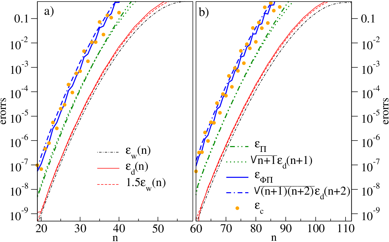
Nonzero $\epsilon_{w}(n)$ causes a finite difference between the discretized HG functions $|\tilde{n}\rangle$ defined by Eq. 46, and the eigenvectors of the discrete harmonic oscillator, $|\tilde{\phi}_{n}\rangle$ . Employing exact diagonalization to calculate $|\tilde{\phi}_{n}\rangle$ we find that

\displaystyle\epsilon_{d}(n)=\left|\left||\tilde{n}\rangle-|\tilde{\phi}_{n}\rangle\right|\right|,

(55)

is proportional to $\epsilon_{w}(n)$ , i.e. $\epsilon_{d}(n)\approx 1.5\epsilon_{w}(n)$ , as illustrated with thin continuous red and dashed red lines in Fig. 4.

Each time the field operators $\tilde{\Phi}$ and $\tilde{\Pi}$ act on the eigenvector $|\tilde{\phi}_{n}\rangle$ of $\tilde{H}_{h}$ , the errors are amplified approximately by a factor of $\sqrt{n+1}$ . This can be understood from Eqs. 49 and 50 when one replaces $|\widetilde{n+1}\rangle$ with $|\tilde{\phi}_{n+1}\rangle+\left(|\widetilde{n+1}\rangle-|\tilde{\phi}_{n+1}\rangle\right)$ . The leading error associated with the finite magnitude of $|\widetilde{n+1}\rangle-|\tilde{\phi}_{n+1}\rangle$ is magnified by a factor $\sqrt{n+1}$ . Numerical calculations agree with this assertion. For example, the state $\tilde{\Pi}|\tilde{\phi}_{n}\rangle$ behaves as $\Pi|n\rangle$ up to an error,

\displaystyle\epsilon_{\Pi}(n)=\left|\left|\tilde{\Pi}|\tilde{\phi}_{n}\rangle-\frac{-i}{\sqrt{2}}\left(\sqrt{n}|\tilde{\phi}_{n-1}\rangle-\sqrt{n+1}|\tilde{\phi}_{n+1}\rangle\right)\right|\right|.

(56)

As shown in Fig. 4 with dash-dot-dot green and dotted green lines, $\epsilon_{\Pi}(n)\approx\sqrt{n+1}\epsilon_{d}(n+1)$ . The same conclusion is valid for the error associated with the behavior of the state $\tilde{\Phi}|\tilde{\phi}_{n}\rangle$ (not shown).

The error associated to the commutation relation, $\left[\tilde{\Phi},\tilde{\Pi}\right]|\tilde{\phi}_{n}\rangle$ , is comparable with the errors associated to the states $\tilde{\Phi}\tilde{\Pi}|\tilde{\phi}_{n}\rangle$ and $\tilde{\Pi}\tilde{\Phi}|\tilde{\phi}_{n}\rangle$ . Figure 4 shows

\displaystyle\epsilon_{\Phi\Pi}(n)=\left|\left|\tilde{\Phi}\tilde{\Pi}|\tilde{\phi}_{n}\rangle-\frac{i}{2}\left(-\sqrt{(n-1)n}|\tilde{\phi}_{n-2}\rangle+\sqrt{(n+1)(n+2)}|\tilde{\phi}_{n+2}\rangle+|\tilde{\phi}_{n}\rangle\right)\right|\right|,

(57)

with a thick solid blue line, and

\displaystyle\epsilon_{c}=\left|\left|\left(\left[\tilde{\Phi},\tilde{\Pi}\right]-i\right)|\tilde{\phi}_{n}\rangle\right|\right|,

(58)

with orange dots. We find (see also the dot-dash-dash blue line) that

\displaystyle\epsilon_{\Phi\Pi}(n)\approx\epsilon_{c}\approx\sqrt{(n+1)(n+2)}\epsilon_{d}(n+2).

(59)

Since $\epsilon_{w}(n,N_{\varphi})$ increases with increasing $n$ , for a finite representation of size $N_{\varphi}$ and cutoff $N_{b}$ , the leading error is of the order of $\epsilon_{w}(N_{b}+2,N_{\varphi})$ . For a given cutoff $N_{b}$ , the error can be reduced exponentially by increasing the number of discretization points $N_{\varphi}$ , $\epsilon\propto\epsilon_{w}(N_{b}+2,N_{\varphi})\leq e^{-\frac{\pi}{4}N_{\varphi}+\frac{\left(2N_{b}+3\right)}{4}\ln N_{\varphi}}$ , as Eq. 54 and the numerical results shown in Fig. 3 imply.

For fixed accuracy, an increase of the low-energy subspace requires an increase of $N_{\varphi}$ . For small $N_{b}/N_{\varphi}$ the dependence between $N_{b}$ and $N_{\varphi}$ at fixed error is given by Eq. 54. The region where the accuracy is of order $\epsilon=10^{-3}\sim 10^{-5}$ is of practical interest for simulations. In this region $N_{b}/N_{\varphi}\in\approx\left[0.3,0.7\right]$ and Eq. 54 overestimates the errors. Numerical investigations and arguments based on the WKB approximation Macridin et al. 2018b; Macridin et al. 2018a indicate that, in this region

\displaystyle N_{\varphi}\approx c_{1}+c_{2}N_{b},

(60)

where $c_{1}$ and $c_{2}$ are accuracy dependent parameters. At fixed accuracy, there is a linear dependence between the size $N_{\varphi}$ of the finite space $\tilde{{\cal{H}}}$ and the boson cutoff number $N_{b}$ . For example, we find that the number of discretization points $N_{\varphi}\approx 32+1.5N_{b}$ for an accuracy $\epsilon=10^{-3}$ Macridin et al. 2018b. In practice, for many problems of interest, such as scalar $\Phi^{4}$ theory and electron-phonon systems, the representation in the field amplitude basis requires only one more qubit per harmonic oscillator than the representation in the boson number basis.

Numerical investigations in the region with the error range $\epsilon\in\left[10^{-5},10^{-3}\right]$ Macridin et al. 2018b, yield the following upper bound for the error associated with the commutation relation (Eq. 58),

\displaystyle\epsilon_{c}<10e^{-\left(0.51N_{\varphi}-0.765N_{b}\right)}.

(61)

In Fig. 3, we show with dotted lines $\epsilon_{w}(n)=\epsilon_{c}(n-2)/\left(1.5\sqrt{n\left(n-1\right)}\right)$ (see the numerical dependence between $\epsilon_{d}$ and $\epsilon_{c}$ in Eq. 59) where $\epsilon_{c}$ is given by Eq. 61.

III.2.2 Representation of the lattice Hilbert space

The construction of the lattice representation is a straightforward extension of the local representation construction. The lattice Hilbert space is a direct product of $N$ local infinite Hilbert spaces,

\displaystyle{\cal{H}}=\prod_{j=1}^{N}\otimes{\cal{H}}_{j}\equiv L^{2}(\mathbb{R}^{N}),

(62)

where $N$ represents the number of the lattice sites. The finite size Hilbert space of dimension $\left(N_{\varphi}\right)^{N}$ ,

\displaystyle\tilde{\cal{H}}=\prod_{j=1}^{N}\otimes\tilde{\cal{H}}_{j},

(63)

with $\tilde{\cal{H}}_{j}$ being the local Hilbert spaces of dimension $N_{\varphi}$ constructed in Section III.2.1, is a representation of the lattice low-energy subspace with maximum $N_{b}$ bosons per site. The Hilbert space $\tilde{\cal{H}}$ is spanned by the vectors

\displaystyle\left\{|\tilde{\varphi}_{i_{1}}\rangle_{1}|\tilde{\varphi}_{i_{2}}\rangle_{2}...|\tilde{\varphi}_{i_{N}}\rangle_{N}\right\},~~~~~~\text{with }~~~~i_{j}=\overline{-\frac{N_{\varphi}-1}{2},\frac{N_{\varphi}-1}{2}}.

(64)

The discrete field operators are defined as

	$\displaystyle\tilde{\Phi}_{j}\|\tilde{\varphi}_{i_{1}}\rangle_{1}..\|\tilde{\varphi}_{i_{j}}\rangle_{j}...\|\tilde{\varphi}_{i_{N}}\rangle_{N}$	$\displaystyle=i_{j}\Delta_{\varphi}\|\tilde{\varphi}_{i_{1}}\rangle_{1}..\|\tilde{\varphi}_{i_{j}}\rangle_{j}...\|\tilde{\varphi}_{i_{N}}\rangle_{N}$		(65)
	$\displaystyle\tilde{\Pi}_{j}\|\tilde{\varphi}_{i_{1}}\rangle_{1}..\|\tilde{\kappa}_{m_{j}}\rangle_{j}...\|\tilde{\varphi}_{i_{N}}\rangle_{N}$	$\displaystyle=m_{j}\Delta_{\kappa}\|\tilde{\varphi}_{i_{1}}\rangle_{1}..\|\tilde{\kappa}_{m_{j}}\rangle_{j}...\|\tilde{\varphi}_{i_{N}}\rangle_{N}$		(66)

where

\displaystyle|\tilde{\varphi}_{i_{1}}\rangle_{1}..|\tilde{\kappa}_{m_{j}}\rangle_{j}...|\tilde{\varphi}_{i_{N}}\rangle_{N}=\frac{1}{\sqrt{N_{\varphi}}}\sum_{i_{j}=-\frac{N_{\varphi}-1}{2}}^{\frac{N_{\varphi}-1}{2}}\sum|\tilde{\varphi}_{i_{1}}\rangle_{1}..|\tilde{\varphi}_{i_{j}}\rangle_{j}...|\tilde{\varphi}_{i_{N}}\rangle_{N}e^{i\frac{2\pi i_{j}m_{j}}{N_{\varphi}}}

(67)

is obtained via a local Fourier transform at site $j$ . The conjugate-field operator can be written as

\displaystyle\tilde{\Pi}_{j}

\displaystyle=m_{0}\tilde{\cal{F}}_{j}\tilde{\Phi}_{j}\tilde{\cal{F}}^{-1}_{j},

(68)

where

\displaystyle\tilde{\cal{F}}_{j}=I_{1}\otimes I_{2}\otimes...I_{j-1}\otimes(\tilde{\cal{F}})_{j}\otimes I_{j+1}...\otimes I_{N}

(69)

is the finite Fourier transform acting on the local Hilbert space $\tilde{\cal{H}}_{j}$ .

On the subspace spanned by

\displaystyle\{|\tilde{\phi}_{n_{1}}\rangle_{1}|\tilde{\phi}_{n_{2}}\rangle_{2}...|\tilde{\phi}_{n_{N}}\rangle_{N}\}_{{n_{1}},{n_{2}},...,{n_{N}}<N_{b}},

(70)

where $|\tilde{\phi}_{n}\rangle_{j}\in\tilde{\cal{H}}_{j}$ is the $n$ ’s’ eigenvector of a discrete harmonic oscillator Hamiltonian (45), the field operators satisfy

\displaystyle\left[\tilde{\Phi}_{i},\tilde{\Pi}_{j}\right]=\delta_{ij}\left(iI_{i}+{\cal{O}}(\epsilon)\right),

(71)

where ${\cal{O}}(\epsilon)$ represents the error of constructing local representations and was discussed in Section III.2.1. With ${\cal{O}}(\epsilon)$ accuracy, the algebra generated by the field operators is isomorphic with the algebra generated by the continuous field operators when restricted to the low-energy subspace defined by $n_{j}<N_{b}$ at every $j$ site.

III.3 Accurately sampled states not contained in the low-energy subspace

We have described how to map a low-energy subspace of the infinite Hilbert space onto a low-energy subspace of a finite Hilbert space. The dimension $N_{\varphi}$ of the local finite Hilbert space depends on the dimension $N_{b}$ of the low-energy subspace and the accuracy $\epsilon$ .

While an accurate representation of the low-energy subspace implies accurate sampling of the low-energy wavefunctions, the converse is not necessarily true. Good sampling of a wavefunction does not imply that the wavefunction belongs to the low-energy subspace. There are functions that can be sampled with $\epsilon$ -accuracy in $N_{\varphi}$ points and do not belong to the low-energy subspace of dimension $N_{b}(N_{\varphi},\epsilon)$ . Since the high-energy subspace projection of these wavefunctions is significant, the actions of the discrete field operators on them yield uncontrollable errors. Therefore, it is important to verify that the system wavefunction has a boson distribution that is below the cutoff. We describe how this can be accomplished with quantum simulations in Section V.

To emphasize this point, we present examples of wavefunctions with small tail weights outside sampling intervals that can be sampled accurately on $N_{\varphi}$ discretization points, but have a significant high-energy weight and therefore cannot be represented accurately on a finite Hilbert space of dimension $N_{\varphi}$ .

For the first example, we consider a band-limited function $f(\varphi)$ (see Eqs. 12 and 13)

\displaystyle f(\varphi)=\sum_{i=-\frac{N_{\varphi}-1}{2}}^{\frac{N_{\varphi}-1}{2}}a_{i}u_{K}(\varphi-\varphi_{i})\,

(72)

where we take $F=K=\sqrt{\pi N_{\varphi}/2}$ , (see Eq. 15), with $N_{\varphi}=64$ . As described in Appendix D, the coefficients $a_{i}$ are chosen such that the behavior as $\varphi\to\infty$ is

\displaystyle f(\varphi)\sim c_{f}\sin\left(\frac{\pi\varphi}{\Delta_{\varphi}}-\frac{\pi}{2}\right)\frac{\Delta_{\varphi}^{8}}{\pi\varphi^{8}}+{\cal{O}}\left(\frac{\Delta_{\varphi}^{10}}{\pi\varphi^{10}}\right),

(73)

where $c_{f}$ is a normalization constant, i.e. the function decays as $|\varphi|^{-8}$ with increasing $|\varphi|$ . The square amplitudes $|f(\varphi)|^{2}$ and $|\hat{f}(\kappa)|^{2}$ are plotted in Fig. 5. For $\varphi<-F$ , we have $|f(\varphi)|^{2}\approx{\cal{O}}(10^{-10})$ as can be seen in Fig. 5-(b). The weight outside the interval $\left[-F,F\right]$ is $||w_{F}^{f}||\approx 1.1\times 10^{-5}$ . Since the function is band-limited, $\hat{f}(\kappa)=0$ for $|\kappa|>K$ . By construction, the Finite Fourier transform connects the sets $\{f(\varphi_{i})\}_{i=\overline{-\left(N_{\varphi}-1\right)/2,\left(N_{\varphi}-1\right)/2}}$ and $\{\hat{f}(\kappa_{p})\}_{p=\overline{-\left(N_{\varphi}-1\right)/2,\left(N_{\varphi}-1\right)/2}}$ without error, since, in the sampling points, the function coincides with the aliased function (see Eqs. 186 and 187).

Despite the small tail weight and perfect sampling, the wavefunction $f(\varphi)$ cannot be represented accurately on a finite Hilbert space of size $N_{\varphi}=64$ . To demonstrate this, we show in Fig. 6-(a) the boson distribution of the wavefunction $f(\varphi)$ ,

\displaystyle p(n)=|\langle n\vphantom{f}|f\vphantom{n}\rangle|^{2}=\left|\int\phi_{n}(\varphi)f(\varphi)d\varphi\right|^{2},

(74)

and in Fig. 6-(b) the weight $1-W_{N_{b}}$ of the high-energy subspace versus the cutoff $N_{b}$ , where

\displaystyle W_{N_{b}}=\sum_{n<N_{b}}p(n).

(75)

The figure indicates a significant boson distribution for $n>N_{b}=30$ . In fact we observe that $50\%$ of the wavefunction belongs to the subspace spanned by boson states with $n>30$ and $20\%$ of the wavefunction belongs to the subspace spanned by boson states with $n>40$ . However, according to the data presented in Fig. 4-(a), the boson number states with $n>30$ cannot be represented with ${\cal{O}}(10^{-5})$ accuracy on $N_{\varphi}=64$ discretization points.

Due to the significant high-energy weight of $f(\varphi)$ , the representation of the function on a finite space with $N_{\varphi}=64$ ,

\displaystyle|\tilde{f}\rangle=\sum_{i=-\frac{N_{\varphi}-1}{2}}^{i=\frac{N_{\varphi}-1}{2}}f(\varphi_{i})|\tilde{\varphi}_{i}\rangle,

(76)

yields uncontrollable errors when measurements are taken. For example, the boson distribution calculated on the finite Hilbert space using the discrete representation $\tilde{f}$ and the harmonic oscillator eigenstates $\tilde{\phi_{n}}$ ,

\displaystyle\tilde{p}(n)=|\langle\tilde{\phi}_{n}\vphantom{\tilde{f}}|\tilde{f}\vphantom{\tilde{\phi}_{n}}\rangle|^{2},

(77)

is different from the real boson distribution given by Eq. 74, as illustrated in Fig. 6-(a).

Since the asymptotic behavior of the wavefunction might impact significantly its boson distribution, we consider a second example obtained by multiplying $f(\varphi)$ with the exponentially decaying function $s(\varphi)$

	$\displaystyle g(\varphi)$	$\displaystyle=c_{g}f(\varphi)s(\varphi),$		(78)
	$\displaystyle s(\varphi)$	$\displaystyle=\frac{1}{\left(e^{-\frac{\varphi+L}{\sigma}}+1\right)^{2}\left(e^{\frac{\varphi-L}{\sigma}}+1\right)^{2}}.$		(79)

In Eq. 78, $c_{g}$ is a normalization constant and, in Eq. 79, we take $\sigma=0.4$ . The function $s(\varphi)$ , plotted in Fig. 5-(d), takes the value $1$ almost everywhere inside the interval $\left[-F,F\right]$ and decays exponentially outside this interval ( $s(\varphi)\propto\mathrm{exp}(-\varphi^{2}/\sigma^{2})$ at large $|\varphi|$ ). Unlike $f(\varphi)$ , which might be considered a specially chosen case, $g(\varphi)$ is a more common example. It is not band-limited or field-limited and has exponentially decaying tails. However, at the scale shown in Fig. 5-(a), the functions $f(\varphi)$ and $g(\varphi)$ are indistinguishable. The difference between $f(\varphi)$ and $g(\varphi)$ can be seen in Fig. 5-(b). The difference between their Fourier transforms can be seen in Fig. 5-(c). The tail weight of $g(\varphi)$ outside $\left[-F,F\right]$ is $||w_{F}^{g}||\approx 6\times 10^{-6}$ . Unlike $\hat{f}(\kappa)$ , the conjugate variable function $\hat{g}(\kappa)$ is not zero for $\kappa>|K|$ . However, its tail weight is small, $||w_{K}^{g}||\approx 6.2\times 10^{-6}$ . Within accuracy ${\cal{O}}(10^{-5})$ , the discrete representation of $g(\varphi)$ is the same as the one for $f(\varphi)$ , $|\tilde{g}\rangle\approx|\tilde{f}\rangle$ .

Despite the different asymptotic behavior of the functions $f(\varphi)$ and $g(\varphi)$ at large argument, the difference between the boson distribution of these two functions functions is very small, indistinguishable on the scale shown in Fig. 6. The differences are noticeable for $n>80$ where the boson weight is small, of the order ${\cal{O}}(10^{-10})$ (not shown). All the conclusions we drew about $f(\varphi)$ are valid for $g(\varphi)$ too. The wavefunction $g(\varphi)$ is not restricted to the low-energy subspace corresponding to $N_{\varphi}=64$ and accuracy ${\cal{O}}(10^{-5})$ and cannot be represented accurately on a finite Hilbert space of size $N_{\varphi}=64$ . The boson distribution $|\langle n\vphantom{g}|g\vphantom{n}\rangle|^{2}$ of the wavefunction $g(\varphi)$ differs from the boson distribution $|\langle\tilde{\phi}_{n}\vphantom{\tilde{g}}|\tilde{g}\vphantom{\tilde{\phi}_{n}}\rangle|^{2}$ of the discrete representation.

These two examples of functions with small tail weight at large argument, one band-limited and having algebraic decay and one with exponential decay, that can be sampled accurately but cannot be restricted to the low-energy subspace, show that the criteria of small weight at large argument is not enough for determining the size of the finite representation. It would be useful to have an estimate of the Hermite-Gauss functions expansion series for almost band-limited and field-limited functions as a function of the tail weights and the cutoff $N_{b}$ ,

\displaystyle\left|\left||f\rangle-\sum_{n=0}^{N_{b}}c_{n}|n\rangle\right|\right|\approx{\cal{E}}(N_{b},||w_{F}^{f}||,||w_{K}^{f}||,...).

(80)

Such an expression could be used to estimate the cutoff $N_{b}$ and the number of the discretization points necessary for an accurate representation by measuring the field and conjugate-field distributions. We are not aware if an estimation like Eq. 80 exists in the literature. It is possible that combining the estimation of the prolate spheroidal wavefunctions expansion of almost band limited functions Landau and Pollak 1962 with the estimation of the Hermite-Gauss function expansion of prolate spheroidal wavefunctions Osipov et al. 2013 would yield an useful expression, but the problem requires further investigation.

IV Sampling parameters and the boson mass choice

As discussed previously, the low-energy subspace of a bosonic field can be mapped accurately onto a low-energy subspace of a finite Hilbert space. The dimension $N_{\varphi}$ of the local finite Hilbert space is monotonically increasing with the low-energy subspace dimension $N_{b}$ . The boson number states and implicitly the cutoff $N_{b}$ are dependent on the mass parameter $m_{0}$ (see Eq. 2). The definition of the finite Hilbert space $\tilde{\cal{H}}$ and of the discrete field operators depends on $m_{0}$ too, as implied by Eqs. 40 and 41. There are many possible finite representations of the bosonic field that correspond to different choices of the boson mass. The optimal representation is the one that requires the smallest cutoff $N_{b}$ for the ground state and for the low-energy excitations of the system.

IV.1 Squeezed boson states

To represent the ground state of a harmonic oscillator with mass $m_{0}$ , the optimal choice for the boson mass is simply $m_{0}$ , because for this choice the ground state has zero bosons (the ground state is the vacuum). However, other choices for the mass parameter can be taken, but they require more discretization points for a specified accuracy, as we discuss below. We work through this case as a prelude to more complicated Hamiltonians where the optimal choice of mass is not obvious.

The Hamiltonian (1) can be re-written as

\displaystyle H_{h}

\displaystyle=\frac{m_{1}}{4}\left(\frac{m_{0}^{2}}{m_{1}^{2}}-1\right)\left(a^{\dagger}_{1}a^{\dagger}_{1}+a_{1}a_{1}\right)+\frac{m_{1}}{4}\left(\frac{m_{0}^{2}}{m_{1}^{2}}+1\right)\left(2a^{\dagger}_{1}a_{1}+1\right).

(81)

where the mass $m_{1}$ -bosons are defined by

\displaystyle a^{\dagger}_{1}=\frac{1}{\sqrt{2}}\left(\sqrt{m_{1}}\Phi-i\frac{1}{\sqrt{m_{1}}}\Pi\right)~~~\text{and}~~~a_{1}=\frac{1}{\sqrt{2}}\left(\sqrt{m_{1}}\Phi+i\frac{1}{\sqrt{m_{1}}}\Pi\right).

(82)

The relation between the mass $m_{1}$ -bosons and the mass $m_{0}$ ones is given by the squeezing operation

\displaystyle a^{\dagger}_{0}=S(r)^{\dagger}a^{\dagger}_{1}S(r)

(83)

where

\displaystyle S(r)=e^{\frac{1}{2}r\left({a_{1}^{\dagger}}^{2}-a^{2}_{1}\right)}~~~\text{and}~~~r=\frac{1}{2}\ln\left(\frac{m_{1}}{m_{0}}\right).

(84)

In the basis $\{|n\rangle_{1}\}_{n}$ , where $|n\rangle_{1}=\frac{1}{\sqrt{n!}}a_{1}^{\dagger n}|0\rangle_{1}$ is the state with $n$ $m_{1}$ -bosons, the harmonic oscillator ground state $|0\rangle$ is a squeezed vacuum state Gerry and Knight 2004,

	$\displaystyle\|0\rangle\equiv\|0\rangle_{0}$	$\displaystyle=S^{\dagger}(r)\|0\rangle_{1}=\sum_{n=0}^{\infty}C_{n}\|n\rangle_{1},$		(85)
	$\displaystyle C_{2n}$	$\displaystyle=\left(-1\right)^{n}\frac{\sqrt{\left(2n\right)!}}{2^{n}n!}\frac{\left(\tanh r\right)^{n}}{\sqrt{\cosh r}},~~~\text{ }~~~C_{2n+1}=0.$		(86)

The magnitude of the coefficients $C_{2n}$ in Eq. 86 decrease rapidly with increasing $n$ . For any small $\epsilon$ a cutoff $N_{b}$ can be introduced such that the the harmonic oscillator ground state has $\epsilon$ probability to have more than $N_{b}$ $m_{1}$ -bosons.

The cutoff $N_{b}$ increases with increasing or decreasing $\frac{m_{1}}{m_{0}}$ . In Fig. 7-(a) we plot the $m_{1}$ -boson distribution, $p\left(n;\frac{m_{1}}{m_{0}}\right)=p\left(n;\frac{m_{0}}{m_{1}}\right)=\left|C_{n}\right|^{2}$ as a function of $n$ for different values of $\frac{m_{1}}{m_{0}}$ . When $m_{1}=m_{0}$ the distribution has $p(0)=1$ and $p(n>1)=0$ , since the ground state is the $m_{0}$ -bosons vacuum. The distribution weight at large $n$ increases with increasing $\frac{m_{1}}{m_{0}}$ or $\frac{m_{0}}{m_{1}}$ . The cutoff $N_{b}$ is defined by requiring that $1-W_{N_{b}}=\epsilon$ , where $W_{N_{b}}$ is the weight of the low-energy subspace spanned by the boson number states below the cutoff $N_{b}$ (see Eq. 75) and $\epsilon$ is the desired truncation error. In Fig. 7-(b) we show $N_{b}$ versus $\epsilon=1-W_{N_{b}}$ for different values of the squeezing parameter $r$ . The cutoff $N_{b}$ increases logarithmically with decreasing $1-W_{N_{b}}$ . In Fig. 7-(c) we show the cutoff $N_{b}$ versus $r$ for different values of $1-W_{N_{b}}$ . The cutoff $N_{b}$ increases exponentially with increasing $r$ , which implies linear dependence of $N_{b}$ on the boson mass $m_{1}$ . Numerical fitting yields $N_{b}\approx\left[-0.595-0.477\ln\epsilon\right]\frac{m_{1}}{m_{0}}$ . Since the number of the discretization points $N_{\varphi}$ needed to represent the low-energy subspace increases monotonically with $N_{b}$ , a boson mass choice $m_{1}\neq m_{0}$ is not optimal.

This same conclusion can be inferred just by analyzing the Nyquist-Shannon sampling parameters of the harmonic oscillator wavefunctions $\phi_{0}(\varphi)$ and $\hat{\phi}_{0}(\kappa)$ . For a given number $N_{\varphi}$ of discretization points, the $m_{0}$ -sampling implies the sampling intervals (see Eqs. 28 and 29)

\displaystyle F_{0}=\sqrt{\frac{\pi N_{\varphi}}{2m_{0}}},~~~~K_{0}=\sqrt{\frac{\pi N_{\varphi}m_{0}}{2}},

(87)

which yield equal tail weights $||w_{F_{0}}^{\phi_{0}}||=||w_{K_{0}}^{\phi_{0}}||$ . For $m_{1}$ -sampling one has

\displaystyle F_{1}=F_{0}\sqrt{\frac{m_{0}}{m_{1}}},~~~~K_{1}=K_{0}\sqrt{\frac{m_{1}}{m_{0}}}.

(88)

For $m_{1}>m_{0}$ , the field sampling interval decreases while the conjugate-field sampling interval increases by a factor $\sqrt{m_{1}/m_{0}}$ . Consequently the tail weight $||w_{F_{1}}^{\phi_{0}}||\gg||w_{F_{0}}^{\phi_{0}}||$ increases exponentially, while $||w_{K_{1}}^{\phi_{0}}||\ll||w_{K_{0}}^{\phi_{0}}||$ decreases exponentially (since the tail weights have an exponential dependence on the sampling intervals’ length). Similarly, when $m_{0}>m_{1}$ the tail weight $||w_{F_{1}}^{\phi_{0}}||\ll||w_{F_{0}}^{\phi_{0}}||$ and $||w_{K_{1}}^{\phi_{0}}||\gg||w_{K_{0}}^{\phi_{0}}||$ . In both cases, because of the large increase of one of the tail weights, the Finite Fourier transform that connects the field and the conjugate-field sampling sets yields a much larger error (see Eqs. 22 and 23) than in the case of $m_{0}$ -sampling. Since the error in constructing the finite Hilbert space representation is proportional to the error introduced by the Finite Fourier transform (see Eq. 46), sampling corresponding to $m_{1}\neq m_{0}$ implies larger errors than $m_{0}$ -sampling.

IV.2 Sampling intervals

The sampling and discretization intervals depend on the boson mass and the number of the discretization points, in accordance with Eqs. 34, 36 and 87. The ratio of the sampling intervals and, as well, the ratio of the discretization intervals, equal the boson mass

\displaystyle m=\frac{K}{F}=\frac{\Delta_{\kappa}}{\Delta_{\varphi}}.

(89)

By definition, the optimal boson mass requires the minimal number of the discretization points for an accurate representation. In principle, for a specified accuracy, the optimal boson mass can be obtained by minimizing the cutoff $N_{b}$ of the wavefunction’s expansion in the boson number basis. However, this is not easy to accomplish, since the extraction of $N_{b}$ from quantum simulations is laborious, as will be discussed in Section V.

Nevertheless, instead of finding the boson mass for optimal representation, one can ask about the boson mass that yields optimal sampling. Adjusting parameters for optimal sampling in quantum simulations is much easier than optimizing for the smallest cutoff $N_{b}$ , as will be discussed in Section V. The sampling accuracy of a wavefunction is determined by the wavefunction behavior outside the field and the conjugate-field sampling intervals. For a specified accuracy $\epsilon$ , the sampling intervals parameters $F$ and $K$ should be chosen such that (see Eq. 8 and Eq. 11)

\displaystyle||w_{F}^{\phi}||=||w_{K}^{\phi}||=\epsilon.

(90)

This choice will provide, via Eq. 15, the minimum number of discretization points required for a sampling approximation with ${\cal{O}}(\epsilon)$ accuracy.

Do the sampling intervals $F$ and $K$ determined by imposing Eq. 90 yield the optimal boson mass through Eq. 89? While we do not know the answer in general, numerical checks show that the answer is yes in many cases. That is the case of the harmonic oscillator, as was already discussed in Section IV.1. We also found the answer to be yes for small size $\Phi^{4}$ scalar field models that we can solve numerically using exact diagonalization methods. In the following, we present two relevant $\Phi^{4}$ scalar field examples .

IV.2.1 Local $\Phi^{4}$ scalar field

The first example is a strong interacting local $\Phi^{4}$ field model, equivalent to an anharmonic oscillator, with the Hamiltonian

\displaystyle H=\frac{\Pi^{2}}{2}+\frac{1}{2}m_{0}^{2}\Phi^{2}+\frac{g}{4!}\Phi^{4}.

(91)

Figure 8 (a) shows the field and the conjugate-field distribution of the ground state of the Hamiltonian (91) for interaction strength $\frac{g}{m_{0}^{3}}=100$ . One effect of the interaction is to narrow the field distribution $|\Phi(\varphi)|^{2}$ and to widen the conjugate-field distribution $|\hat{\Phi}(\kappa)|^{2}$ compared to the non-interacting case. The interaction also affects the field distributions behavior at large argument, as can be seen in the insets. The wavefunction $\hat{\Phi}(\kappa)$ has an oscillatory behavior at large $|\kappa|$ .

Optimal sampling implies a ratio ( $\propto K/F$ ) larger than the bare mass $m_{0}$ , because the $|\hat{\Phi}(\kappa)|^{2}$ distribution is wider than the $|\Phi(\varphi)|^{2}$ one. Figure 8-(b) shows the ratio of the sampling intervals $\frac{1}{m_{0}}\frac{K}{F}$ versus the tail weight $\epsilon$ , where $F$ and $K$ are determined by Eq. 90. The ratio $\frac{1}{m_{0}}\frac{K}{F}$ is dependent on $\epsilon$ , and increases logarithmically (and non-uniformly due to the oscillatory behavior of $|\hat{\Phi}(\kappa)|^{2}$ ) with increasing the accuracy, from $\frac{1}{m_{0}}\frac{K}{F}\approx 4$ for an accuracy $\epsilon=10^{-3}$ to $\frac{1}{m_{0}}\frac{K}{F}\approx 6$ for $\epsilon=10^{-9}$ . The number of discretization points $N_{\varphi}=\lceil 2KF/\pi\rceil$ , necessary to sample the local $\Phi^{4}$ field ground state increases logarithmically with increasing the accuracy, as can be seen in Fig. 8-(c).

To calculate the boson distribution, we diagonalize numerically the Hamiltonian (91) in the boson number basis. Figure 8-(d) shows the boson distribution, $p(n)$ , as function of $n$ for different choices of the boson mass. In all cases, the boson distribution decreases rapidly with increasing number of bosons. We find that the largest decreasing slope occurs when the boson mass $m/m_{0}\in\approx\left[4,8\right]$ . Figure 8-(e) shows the cutoff $N_{b}$ versus the boson mass for different truncation errors $1-W_{N_{b}}$ . Remember that $1-W_{N_{b}}$ , with $W_{N_{b}}$ defined by Eq. 75, is the weight of the subspace spanned by the boson number states above the cutoff. The optimal boson mass occurs at the minimum of $N_{b}(m/m_{0})$ . For a truncation error $1-W_{N_{b}}\approx 10^{-5}$ we find $m/m_{0}\approx 4$ . The optimal boson mass increases to $m/m_{0}\approx 8$ with decreasing the truncation error to $1-W_{N_{b}}\approx 10^{-12}$ .

The optimal boson mass determined by minimizing $N_{b}$ is in agreement with the boson mass calculated by minimizing the sampling errors of $\Phi(\varphi)$ and $\hat{\Phi}(\kappa)$ . Since the truncation error given by the weight of the subspace spanned by the boson number states above the cutoff is not the same as the sampling error determined by the wavefunction’s weight outside the sampling intervals, a quantitative comparison between $\frac{K}{F}$ plotted in Fig. 8-(b) and an optimal boson mass extracted from Fig. 8-(e) is not meaningful. However, we found in both cases that the optimal boson mass is in the same range, $m/m_{0}\in\left[4,8\right]$ , and that it increases when increasing the accuracy of the approximation.

IV.2.2 Two-site $\Phi^{4}$ scalar field

The next example is a two site $\Phi^{4}$ field theory,

\displaystyle H=\sum_{i=1,2}\left(\frac{\Pi_{i}^{2}}{2}+\frac{1}{2}m_{0}^{2}\Phi_{i}^{2}+\frac{g}{4!}\Phi_{i}^{4}\right)-h\Phi_{1}\Phi_{2},

(92)

with $m_{0}^{2}=-1$ , $\displaystyle\frac{g}{|m_{0}|^{3}}=2$ and $\displaystyle\frac{h}{|m_{0}|^{2}}=1$ . The coupling between the fields operators at neighboring sites is a consequence of the gradient term, $(\nabla\Phi)^{2}$ , present in the Lagrangian of a continuous $\Phi^{4}$ field theory. Although no real broken symmetry occurs for a two-site system, the negative value of $m_{0}^{2}$ yields interesting behavior relevant for exploring models with a broken symmetry phase. The field in the ground state has a two-peak structure and the excitation gap is small.

The local field distribution,

\displaystyle p_{1}(\varphi)=\langle\varphi\vphantom{\varphi}|\rho_{1}|\varphi\vphantom{\varphi}\rangle,

(93)

and the local conjugate-field distribution

\displaystyle p_{1}(\kappa)=\langle\kappa\vphantom{\kappa}|\rho_{1}|\kappa\vphantom{\kappa}\rangle,

(94)

are plotted in Fig. 9-(a). In Eqs. 93 and 94 $\rho_{1}$ is the local density matrix

\displaystyle\rho_{1}

\displaystyle=\text{Tr}_{2}(|\phi\rangle\langle\phi|),

(95)

obtained by tracing out the degrees of freedom at site $2$ , while $|\phi\rangle$ in Eq. 95 is the ground state of the Hamiltonian (92).

Since the sampling errors of lattice wavefunctions depend on the tail weights of the local distributions (see Section B.2), the sampling intervals lengths are determined by imposing $w_{1F}^{\phi}=w_{1K}^{\phi}=\epsilon$ , where

	$\displaystyle{w_{1F}^{\phi}}^{2}$	$\displaystyle=\int_{-\infty}^{-F}d\varphi\langle\varphi\vphantom{\varphi}\|\rho_{1}\|\varphi\vphantom{\varphi}\rangle+\int_{F}^{\infty}d\varphi\langle\varphi\vphantom{\varphi}\|\rho_{1}\|\varphi\vphantom{\varphi}\rangle,$		(96)
	$\displaystyle{w^{\phi}_{1K}}^{2}$	$\displaystyle=\int_{-\infty}^{-K}\langle\kappa\vphantom{\kappa}\|\rho_{1}\|\kappa\vphantom{\kappa}\rangle d\kappa+\int_{K}^{\infty}\langle\kappa\vphantom{\kappa}\|\rho_{1}\|\kappa\vphantom{\kappa}\rangle d\kappa,$		(97)

(see also Eqs. 181 and 169). As can be seen in the inset of Fig. 9-(a), the local field distribution decays more rapidly with increasing argument than the conjugate-field one. The ratio of the sampling intervals widths, $\displaystyle\frac{1}{|m_{0}|}\frac{K}{F}$ , versus the tail weight is plotted in Fig. 9-(b). It increases logarithmically with decreasing tail weight, from $\displaystyle\frac{1}{|m_{0}|}\frac{K}{F}\approx 1.2$ when the tail weight is $\epsilon\approx 10^{-4}$ to $\displaystyle\frac{1}{|m_{0}|}\frac{K}{F}\approx 2$ for a tail weight $\epsilon\approx 10^{-12}$ . The number of discretization points, $N_{\varphi}=\lceil\frac{2}{\pi}FK\rceil$ , increases logarithmically with the accuracy, as shown in Fig. 9-(c).

The local boson distribution,

\displaystyle p_{1}(n)=\langle n\vphantom{n}|\rho_{1}|n\vphantom{n}\rangle,

(98)

for different choices of the boson mass is shown in Fig. 9-(d). The boson distribution decreases rapidly with increasing number of bosons. The largest decreasing slope is observed for ${m}/{|m_{0}|}\approx 2$ . The cutoff $N_{b}$ versus the boson mass is shown in Fig. 9-(e) for different values of the truncation error $1-W_{N_{b}}$ . For a truncation error $1-W_{N_{b}}\approx 10^{-5}$ we find the optimal boson mass to be $m/|m_{0}|\approx 1.2$ . The optimal boson mass increases to $m/|m_{0}|\approx 2$ with decreasing the truncation error to $1-W_{N_{b}}\approx 10^{-12}$ .

As in the case of the local $\Phi^{4}$ field example, the boson optimal mass calculated by minimizing $N_{b}$ is in agreement with the boson mass that minimizes the sampling errors of the local field distributions $p_{1}(\varphi)$ and $p_{1}(\kappa)$ . In both cases, the boson mass is in the same range, $m/|m_{0}|\in\left[1.2,2\right]$ , and it increases when increasing the accuracy of the approximation.

Note that the optimal mass from our analysis is not determined by the standard deviation of the field distributions but by the field and conjugate-field distributions’ behavior at large argument. The ratio of the standard deviations in some mean-field theory approaches is related to the value of the boson mass. Our results suggest that the mean-field solutions obtained in this way are not very good approximations to the optimal mass.

V Post-simulation discretization validation and parameters adjustment

For an accurate simulation, the low-energy subspace should be large enough to contain the relevant physics. The number $N_{\varphi}$ of discretization points per lattice site and the boson mass determine the low-energy subspace, but the optimal values for these parameters are not known a priori. Therefore, it is important to determine a posteriori whether the chosen simulation’s parameters are good and to have procedures to adjust them for optimal performance.

Note that when sufficient quantum computational resources are available, in order to estimate the accuracy of the simulation’s results, one can run simulations for subsequently increasing values of $N_{\varphi}$ and analyze the results’ convergence properties. However, this approach does not provide direct information about optimal discretization intervals and likely will result in sub-optimal use of the available resources.

V.1 Local measurements

The results of a quantum simulation are obtained by measuring the state of the qubits in the computational basis. Not all information about the system is easily accessible from quantum simulations. To validate the choice of discretization parameters in our simulation, we only need measurements of the local field distribution, the local conjugate-field distribution and the local boson distribution. Fortunately, these observables can be measured relatively easily. We discuss their measurements below.

The implementation of quantum algorithms for bosonic fields is described at length in Refs. Macridin et al. 2018a; Macridin et al. 2018b; Li et al. 2021. Here we present only the minimum information necessary to understand the measurements methods. For every lattice site, $n_{q}=\log(N_{\varphi})$ qubits are assigned and the discrete field eigenvector $|\tilde{\varphi}_{i}\rangle_{j}$ is mapped to

\displaystyle|\tilde{\varphi}_{i}\rangle_{j}\equiv|x^{i}_{0},...x^{i}_{n_{q}-1}\rangle_{j},

(99)

where $x^{i}_{r}\in\{0,1\}$ and $j=\overline{1,N}$ is the site label. The field operators (see Eq. 40 and Eq. 65) are defined by

\displaystyle\tilde{\Phi}_{j}|\tilde{\varphi}_{i}\rangle_{j}=\varphi_{i}|\tilde{\varphi}_{i}\rangle_{j}~~~\text{ with }~~~\varphi_{i}=\Delta_{\varphi}\left(\sum_{r=0}^{n_{q}-1}2^{r}x^{i}_{r}-\frac{N_{\varphi}-1}{2}\right).

(100)

The field distribution at site $j$ is given by

\displaystyle p_{j}(\varphi_{i})=\langle\tilde{\varphi}_{i}\vphantom{\tilde{\varphi}_{i}}|\rho_{j}|\tilde{\varphi}_{i}\vphantom{\tilde{\varphi}_{i}}\rangle,

(101)

and is obtained by the direct measurement of the qubits assigned to represent the field at site $j$ , as shown in Fig. 10-(a).

The conjugate-field distribution at site $j$ is given by

\displaystyle p_{j}(\kappa_{p})=\langle\tilde{\kappa}_{p}\vphantom{\tilde{\kappa}_{p}}|\rho_{j}|\tilde{\kappa}_{p}\vphantom{\tilde{\kappa}_{p}}\rangle,

(102)

where $\{|\tilde{\kappa}_{p}\rangle_{j}\}_{p}$ are obtained by applying a local Fourier transform (i.e. a $n_{q}$ -qubit Fourier transform at site $j$ ) to $\{|\tilde{\varphi}_{i}\rangle_{j}\}_{i}$ , as described by Eq. 43. The measurement of this distribution requires an inverse Fourier transform, $\tilde{\cal{F}}^{-1}$ (see Eq. 42), at site $j$ before measuring the qubits, as shown in Fig. 10-(b).

The finite representation of the boson occupation number distribution (i.e. the probability of the discrete harmonic oscillator eigenstates) at site $j$ is given by

\displaystyle p_{j}(n)=\langle\tilde{\phi}_{n}\vphantom{\tilde{\phi}_{n}}|\rho_{j}|\tilde{\phi}_{n}\vphantom{\tilde{\phi}_{n}}\rangle.

(103)

If we write the system’s wavefunction as

\displaystyle|\phi\rangle=\sum_{e}\sum_{n=0}^{N_{\varphi}-1}c_{en}|e\rangle|\tilde{\phi}_{n}\rangle_{j},

(104)

where $\{|e\rangle\}$ is an arbitrary basis for the whole system with the site $j$ excluded, the boson distribution is

\displaystyle p_{j}(n)=\sum_{e}|c_{en}|^{2}.

(105)

The probability to have bosons above the cutoff $N_{b}$ is given by

\displaystyle\epsilon_{H}=\sum_{n=N_{b}}^{N_{\varphi}-1}p_{j}(n)=\sum_{e}\sum_{n=N_{b}}^{N_{\varphi}-1}|c_{en}|^{2}.

(106)

The bosonic field representation is accurate when $\epsilon_{H}$ is negligible.

We present two methods for the measurement of the local boson distribution. The first method employs quantum state tomography (QST) for the local density matrix $\rho_{j}$ . As described in Altepeter et al. 2004; Nielsen and Chuang 2010, $\rho_{j}$ can be written as

\displaystyle\rho_{j}=\frac{1}{2^{n_{q}}}\sum_{v_{0},...v_{n_{q}-1}=0}^{3}s_{v_{0},...v_{n_{q}-1}}P_{v_{0},...v_{n_{q}-1}}.

(107)

The Pauli strings $P_{v_{0},...v_{n_{q}-1}}\equiv\sigma^{j}_{v_{0}}\otimes\sigma^{j}_{v_{1}}\otimes...\otimes\sigma^{j}_{v_{n_{q}-1}}$ are products of Pauli matrices. The single-qubit operator $\sigma^{j}_{v_{q}}$ , acting on the qubit $q\in\left\{0,1,...,n_{q}-1\right\}$ belonging to the local register at site $j$ , takes four possible values, $\sigma^{j}_{v_{q}}\in\{I,\sigma_{x},\sigma_{y},\sigma_{z}\}$ . The coefficients $s_{v_{0},...v_{n_{q}-1}}=\text{Tr}\left(P_{v_{0},...v_{n_{q}-1}}\rho_{j}\right)$ are determined by measuring the corresponding Pauli strings. Similar measurements of the Pauli strings are also employed in Variational Quantum Eigensolver algorithms McClean et al. 2016. Since the number of the independent coefficients defining $\rho_{j}$ is $4^{n_{q}}-1$ , the number of measurements required for QST scales exponentially with $n_{q}$ . This put a severe limitation on QST with large $n_{q}$ Cramer et al. 2010; Lanyon et al. 2017; Titchener et al. 2018. However, the current experimental development Häffner et al. 2005; Song et al. 2017; Titchener et al. 2018 indicates that QST for $n_{q}\leq 8$ (which we believe is large enough for addressing most interesting boson problems) will be feasible in the near future.

Once the local density matrix is determined, its elements in the computational basis can be easily calculated, since this implies evaluating the matrix elements of the Pauli strings in the computational basis. Finally, the boson distribution is given by

\displaystyle p_{j}(n)=\sum_{i,l=0}^{N_{\varphi}-1}\langle\tilde{\phi}_{n}\vphantom{\tilde{\varphi}_{i}}|\tilde{\varphi}_{i}\vphantom{\tilde{\phi}_{n}}\rangle\langle\tilde{\varphi}_{i}\vphantom{\tilde{\varphi}_{l}}|\rho_{j}|\tilde{\varphi}_{l}\vphantom{\tilde{\varphi}_{i}}\rangle\langle\tilde{\varphi}_{l}\vphantom{\tilde{\phi}_{n}}|\tilde{\phi}_{n}\vphantom{\tilde{\varphi}_{l}}\rangle,

(108)

where the coefficients $\langle\tilde{\phi}_{n}\vphantom{\tilde{\varphi}_{i}}|\tilde{\varphi}_{i}\vphantom{\tilde{\phi}_{n}}\rangle$ are obtained from the exact diagonalization of the discrete harmonic oscillator Hamiltonian (45).

The second method for the measurement of the boson distribution at the lattice site $j$ employs quantum phase estimation (QPE) Nielsen and Chuang 2010; Cleve et al. 1998 measurements for the discrete harmonic oscillator

\displaystyle\tilde{H}_{h1}

\displaystyle=\frac{1}{2}\tilde{\Pi}^{2}+\frac{1}{2}m_{0}^{2}\tilde{\Phi}^{2}-\frac{1}{2}m_{0}=H_{h}-\frac{1}{2}m_{0},

(109)

where we subtract the constant term $\frac{1}{2}m_{0}$ for convenience. The eigenvalues of the Hamiltonian (109) have the following property (within the desired accuracy of the finite representation approximation)

	$\displaystyle\tilde{E}_{n}=m_{0}n,~~~~\text{for}~~~n<N_{b},$		(110)
	$\displaystyle\tilde{E}_{n}\neq m_{0}n,~~~~\text{for}~~~n\geq N_{b}.$		(111)

For example, see the eigenvalues of the discrete harmonic oscillator for $N_{\varphi}=64$ and $N_{\varphi}=128$ plotted in Fig.1-(a) of Ref Macridin et al. 2018b.

The time evolution operator corresponding to Hamiltonian (109)

\displaystyle U(\theta)\equiv e^{-i2\pi\theta H_{h1}}

(112)

can be implemented using Trotterization methods, as described in Ref Macridin et al. 2018a; Macridin et al. 2018b; Li et al. 2021. The operator (112) acts only on the $n_{q}$ qubits assigned to the field at the site $j$ .

The implementation of the phase estimation algorithm is illustrated in Fig. 10-(c). An ancillary register of $n_{r}$ qubits is used. On every ancillary qubit, a Hadamard gate is applied. Next, for every qubit $m$ from the ancillary register (with $m=\overline{0,n_{r}-1}$ ), a control- $U(2^{m}\theta)$ gate, acting on the ancilla qubit $m$ and the local field register at site $j$ , is applied.

The state of the system together with the ancillas changes from

\displaystyle|\phi\rangle|0\rangle_{a}=\sum_{e}\sum_{n=0}^{N_{\varphi}-1}c_{en}|e\rangle|\tilde{\phi}_{n}\rangle_{j}|0\rangle_{a},

(113)

where $|0\rangle_{a}$ is the ancillary register state, to

\displaystyle\sum_{e}\sum_{n=0}^{N_{\varphi}-1}c_{en}|e\rangle|\tilde{\phi}_{n}\rangle_{j}\frac{1}{2^{\frac{n_{r}}{2}}}\sum_{x=0}^{2^{n_{r}}-1}|x\rangle_{a}e^{-i2\pi\theta\tilde{E}_{n}x},

(114)

after applying the Hadamard and the $CU$ operators. In Eq. 114, $|x\rangle_{a}$ is the binary representation on qubits of the integer $x=\overline{0,2^{n_{r}}-1}$ . To distinguish between the phase factors corresponding to all eigenvalues of the Hamiltonian (109), the parameter $\theta$ should be chosen such that

\displaystyle\theta<\frac{1}{\Delta E},~~~\text{where}~~\Delta E=\max_{n}{\tilde{E}_{n}}-\min_{n}{\tilde{E}_{n}}

(115)

is the range of the Hamiltonian (109) spectrum.

After the Quantum Fourier transform is applied on the ancilla register, the state described previously by Eq. 114 becomes

\displaystyle|\chi\rangle\equiv\sum_{e}\sum_{n=0}^{N_{\varphi}-1}\sum_{k=0}^{2^{n_{r}}-1}c_{en}a_{nk}|e\rangle|\tilde{\phi}_{n}\rangle_{j}|k\rangle_{a}

(116)

where $|k\rangle_{a}$ is the binary representation on qubits of the integer $k=\overline{0,2^{n_{r}}-1}$ and

\displaystyle a_{nk}=\frac{1}{2^{n_{r}}}\sum_{x=0}^{2^{n_{r}}-1}e^{-i\frac{2\pi}{2^{n_{r}}}\left(2^{n_{r}}\theta\tilde{E}_{n}-k\right)x}.

(117)

The probability to measure the integer $k$ on the ancilla register is given by

\displaystyle p(k)=\sum_{e}\sum_{n=0}^{N_{\varphi}-1}|c_{en}a_{nk}|^{2}.

(118)

If we choose

\displaystyle\theta

\displaystyle=\frac{1}{m_{0}2^{n_{r}}},

(119)

then

\displaystyle a_{nk}=\frac{1}{2^{n_{r}}}\sum_{x=0}^{2^{n_{r}}-1}e^{-i\frac{2\pi}{2^{n_{r}}}\left(\frac{\tilde{E}_{n}}{m_{0}}-k\right)x}.

(120)

The choice of $\theta$ given by Eq. 119 is convenient since $\tilde{E}_{n}/m_{0}=n$ for $n<N_{b}$ . Thus, for $n<N_{b}$ Eq. 117 is a Kronecker delta function, $a_{nk}=\delta_{nk}$ . The probability to measure an integer $k\geq N_{b}$ in the ancilla register reduces to

\displaystyle p(k)=\sum_{e}\sum_{n=N_{b}}^{N_{\varphi}-1}|c_{en}|^{2}|a_{nk}|^{2},~~~~\text{for}~~~k\geq N_{b},

(121)

since the terms in Eq. 118 with $n<N_{b}$ are zero. Since $|a_{nk}|\leq 1$ (see Appendix E), we have the following inequality

\displaystyle p(k)\leq\sum_{e}\sum_{n=N_{b}}^{N_{\varphi}-1}|c_{en}|^{2}=\epsilon_{H},~~~~\text{for}~~~k\geq N_{b}.

(122)

For any $k\geq N_{b}$ , the probability to measure $k$ is smaller than the probability to have more than $N_{b}$ bosons. Thus

\displaystyle\epsilon_{H}\geq\max_{k\geq N_{b}}p(k)\equiv p_{1\text{max}}.

(123)

The probability to measure any integer $k\geq N_{b}$ in the ancilla register is given by

\displaystyle p_{\text{all}}=\sum_{k=N_{b}}^{2^{n_{r}}-1}p(k)=\sum_{e}\sum_{n=N_{b}}^{N_{\varphi}-1}|c_{en}|^{2}\sum_{k=N_{b}}^{2^{n_{r}}-1}|a_{nk}|^{2}\geq\frac{4}{\pi^{2}}\sum_{e}\sum_{n=N_{b}}^{N_{\varphi}-1}|c_{en}|^{2}=\frac{4}{\pi^{2}}\epsilon_{H}.

(124)

In Eq. 124, we used

\displaystyle\sum_{k=N_{b}}^{2^{n_{r}}-1}|a_{nk}|^{2}\geq\max_{k\geq N_{b}}|a_{nk}|^{2}\geq\frac{4}{\pi^{2}}~~~~\text{for}~~~n>N_{b},

(125)

which is proven in Appendix E (see Eq. 206).

Combining Eq. 123 and Eq. 124, the probability to have more than $N_{b}$ bosons is bounded as

\displaystyle p_{1\text{max}}\leq\epsilon_{H}\leq\frac{\pi^{2}}{4}p_{\text{all}}.

(126)

According to Eq. 126, the discretization parameters $N_{\varphi}$ and $m_{0}$ used for bosonic field representation are valid if there is a negligible probability to measure integers larger than the cutoff $N_{b}(N_{\varphi})$ on the ancillary registry.

$N_{\varphi}$	32	64	128	256	512	1024
$\Delta E/m_{0}$	42.319	89.396	185.376	379.976	772.944	1564.233
$N_{b}$ ( $\epsilon_{c}<10^{-4}$ )	10	30	74	164	353	741

Table 1: Middle row: Energy range of the discrete harmonic oscillator for different values of

N_{\varphi}

, calculated using exact diagonalization. Bottom row: Boson cutoff number corresponding to the commutation relation error ( Eq. 58)

\epsilon_{c}\approx 10^{-4}

The size of the ancillary register is determined by Eq. 115 and Eq. 119,

\displaystyle n_{r}

\displaystyle\geq\log\left(\left[\frac{\Delta E}{m_{0}}\right]\right).

(127)

The number of ancillary qubits scales logarithmically with the energy range of the discrete harmonic oscillator Hamiltonian. The values of the energy range $\Delta E$ corresponding to different $N_{\varphi}$ are given in Table 1. We find that $\Delta E/m_{0}<2N_{\varphi}$ for $N_{\varphi}\leq 1024$ (and probably true for larger values of $N_{\varphi}$ as well but numerical checks are necessary for confirmation). In practice the number of ancillary qubits required for the QPE register is

\displaystyle n_{r}=n_{q}+1.

(128)

Measuring energies in QPE algorithms with $2^{-n}$ accuracy and with $1-\epsilon$ probability requires registers of size $n_{r}=n+\log\left[2+1/(2\epsilon)\right]$ Nielsen and Chuang 2010; Cleve et al. 1998, thus larger than in our case when $\epsilon\lesssim 10^{-2}$ . In our case, the goal of the QPE measurement is not to estimate the energies of $H_{h}$ (which we know from exact diagonalization of the finite Hamiltonian matrix) but to measure the boson distribution and especially the probability to have states with the number of bosons larger than $N_{b}$ . When the probability to have bosons above the cutoff is negligible, i.e. $\epsilon_{H}\approx 0$ , the boson distribution can be measured with high precision. This is true because the energies of the states with $n<N_{b}$ are proportional to $n$ (see Eq. 110), Eq. 120 becomes a Kronecker delta function and the probability to measure $k<N_{b}$ on the ancillary register becomes equal to the probability to have $n$ bosons (see Eq. 105),

\displaystyle p(k=n)=\sum_{e}|c_{en}|^{2}=p_{j}(n)~~~\text{for}~~~k<N_{b}~~~\text{when}~~\epsilon_{H}=0.

(129)

V.2 Simulation guideline for parameters’ validation and adjustment

In this section, we present a guideline for quantum simulations of bosonic fields. The main goal is to provide a practical procedure for adjusting $N_{\varphi}$ and boson mass $m$ for optimal performance. Let’s assume for now that the system has translational symmetry and the local measurements yield identical results at all sites.

•

If $10$ or less bosons per site is expected to be adequate to capture the low-energy physics, start with $N_{\varphi}=32$ discretization points per lattice site. Otherwise start with a larger $N_{\varphi}$ . Equation (61) can be used to determine the dependence $N_{b}(N_{\varphi},\epsilon)$ . In Table 1 we provide the value of $N_{b}$ for different $N_{\varphi}$ when the accuracy is of order ${\cal{O}}(10^{-4})$ .
•

Start with a boson mass $m=m_{0}+\delta m$ , where $m_{0}$ is the bare mass and $\delta m$ is the mean-field contribution.
•

After the system state is prepared on qubits, measure the local field distribution, $p_{j}(\varphi_{i})$ , and the conjugate-field distribution, $p_{j}(\kappa_{p})$ at the arbitrary site $j$ , as described in Section V.1.

•

Determine the coefficients $\beta_{\varphi}$ and $\beta_{\kappa}$ such that the probability to measure the field outside the range $\left[-\beta_{\varphi}F,\beta_{\varphi}F\right]$ and, respectively, the probability to measure the conjugate-field outside the range $\left[-\beta_{\kappa}K,\beta_{\kappa}K\right]$ are smaller than $\epsilon$ ,

	$\displaystyle\sum_{i\text{ for }\|\varphi_{i}\|>\beta_{\varphi}F}p_{j}(\varphi_{i})<\epsilon$		(130)
	$\displaystyle\sum_{p\text{ for }\|\kappa_{p}\|>\beta_{\kappa}K}p_{j}(\kappa_{p})<\epsilon.$		(131)

If both $\beta_{\varphi}\leq f_{c}$ and $\beta_{\kappa}\leq f_{c}$ the wavefunction sampling is accurate. The parameter $0<f_{c}<1$ should be chosen to ensure confidence that the distribution weights at large argument are $\epsilon$ small. When $f_{c}$ is very large the confidence is low and when $f_{c}$ is very small resources are wasted. We believe that an acceptable range value for $f_{c}$ is $\left[0.6,0.8\right]$ .

The factors $\beta_{\varphi}$ and $\beta_{\kappa}$ can be modified by changing the mass factor since they depend on the intervals’ widths $F\propto m^{-1/2}$ and $K\propto m^{1/2}$ (see Eq. 87). A change of the boson mass by a factor $\mu$ , $m\rightarrow\mu m$ , implies $\beta_{\varphi}\rightarrow\sqrt{\mu}\beta_{\varphi}$ and $\beta_{\kappa}\rightarrow\left(1/\sqrt{\mu}\right)\beta_{\kappa}$ .

•

If $\beta_{\varphi}\beta_{\kappa}\leq f_{c}^{2}$ and $\beta_{\varphi}\approx\beta_{\kappa}$ the guess of the initial mass was close to optimal. If $\beta_{\varphi}\beta_{\kappa}\leq f_{c}^{2}$ and $\beta_{\varphi}\not\approx\beta_{\kappa}$ adjust the boson mass by multiplying it with a factor of $\mu=\beta_{\kappa}/\beta_{\varphi}$ . The new boson mass determines the optimal sampling discretization intervals.
•

The case $\beta_{\varphi}\beta_{\kappa}>f_{c}^{2}$ means that both the field and the conjugate-field distributions close to the sampling intervals’ edges are significant and cannot be adjusted properly by increasing one sampling interval and decreasing the other via boson mass scaling. The number $N_{\varphi}$ of the discretization points should be increased by at least a factor of $\beta_{\varphi}\beta_{\kappa}/f_{c}^{2}$ .

At this point the parameters $N_{\varphi}$ and $m$ are good for optimal field sampling. However, as shown in Section III.3, accurate field sampling does not necessary implies wavefunction containment to the low-energy subspace.
•

Measure the local boson distribution as described in Section V.1.
•

If the probability to measure integers $k\geq N_{b}$ are larger than $\epsilon$ , increase $N_{\varphi}$ (and implicitly $N_{b}(N_{\varphi},\epsilon)$ ) until the probability to measure integers $k\geq N_{b}$ are smaller than $\epsilon$ .

At this point the finite representation of the bosonic field defined by the parameters $N_{\varphi}$ and $m$ should be close to optimal for an accuracy ${\cal{O}}(\epsilon)$ .

In case the wavefunction has no translational symmetry, measurements at all sites are necessary for the validation and adjustment of the discretization parameters. The parameters $N_{\varphi}$ and $m$ should be chosen to provide accurate sampling and a boson distribution contained to the low-energy subspace at all sites. In this case, the global optimal $m$ might not be optimal at every site.

In many simulations, the system’s wavefunction changes in time under the action of the evolution operators. This might be the case for adiabatic continuation or for studying non-equilibrium physics, for example. In principle, measurements for the validation of the discretization parameters should be taken at every time step to make sure that the number of bosons above the cutoff is always smaller than $\epsilon$ . However, in practice, it is not necessary to take discretization validation measurements at every Trotter step. The effect of one Trotter step is of the order of the step size and, therefore, is small. Likely, it will be sufficient to take discretization validation measurements at a rather small number of time points, as long as the boson distribution is well below $N_{b}$ for these measurements.

Use of the optimal parameters will yield the highest precision results for the computational resources available, but this can be challenging in practice. However, accurate, error-controlled quantum simulations can still be performed without adjusting the parameters to their optimal value as long as the problem we address can be restricted to the low-energy subspace. Adjusting the boson mass to the one optimizing the sampling of the wavefunction might increase the precision of the simulations even when the mass is not optimal.

VI Discussion of Future Applications

In this paper, we used the boson number basis to construct a local finite Hilbert space. A low-energy subspace was defined by introducing a cutoff in this basis. A different denumerable basis, for example $\{|\alpha_{n}\rangle\}$ , might be considered for constructing a finite representation, following a similar procedure. However, this change is not trivial, and would require the investigation of the Nyquist-Shannon sampling properties of $\langle\varphi\vphantom{\alpha_{n}}|\alpha_{n}\vphantom{\varphi}\rangle$ and $\langle\kappa\vphantom{\alpha_{n}}|\alpha_{n}\vphantom{\kappa}\rangle$ , knowledge of the recurrence relations for $\varphi\langle\varphi\vphantom{\alpha_{n}}|\alpha_{n}\vphantom{\varphi}\rangle$ and $\kappa\langle\kappa\vphantom{\alpha_{n}}|\alpha_{n}\vphantom{\kappa}\rangle$ , (similar to the ones given by Eq. 26 and, respectively, Eq. 27) and measurement methods for the local distribution $\langle\alpha_{n}\vphantom{\alpha_{n}}|\rho_{j}|\alpha_{n}\vphantom{\alpha_{n}}\rangle$ . We mention this as a topic for future investigation.

Quantum mechanical problems written in the first quantization formalism can be simulated on a quantum computer by employing the discretization methods developed for the bosonic fields. The position $X_{j}$ and the momentum $P_{j}$ operators (here $j$ is an arbitrary label) entering the first quantization Hamiltonian $H(X_{1},X_{2},..,P_{1},P_{2}...)$ play the same role as the field operators $\Phi$ and $\Pi$ , since they obey the canonical commutation relation $\left[X_{j},P_{l}\right]=iI\delta_{jl}$ . The field variable $\varphi$ becomes the position variable $x$ while the conjugate-field variable $\kappa$ becomes the momentum variable $p$ . The system’s wavefunction is discretized in the position and momentum bases. For a general interaction potential $V(X_{1},X_{2},..)$ , a qubit implementation of the corresponding Trotter step operator requires the calculation of the phase factor proportional to $V(x_{1},x_{2},..)$ for each qubit configuration $|x_{1},x_{2},...\rangle$ . This can be challenging when the computation resources are finite, being of similar difficulty as designing a quantum circuit to calculate the function $V(x_{1},x_{2},..)$ Häner et al. 2018; Bhaskar et al. 2015. However, when the potential can be approximated by a truncated Taylor expansion, the implementation reduces to a number of Trotter steps for the monomial terms appearing in the expansion. The Trotter step corresponding to a monomial term with degree $r$ (for example $X_{i}X_{i+1}...X_{i+r}$ ) requires ${\cal{O}}(n_{q}^{r})$ two-qubit gates Macridin et al. 2018b. Special care should also be taken to ensure that the number of the discretization points is large enough such that the action of $V(X_{1},X_{2},..)$ does not violate the low-energy subspace constraints.

As for many quantum algorithms, the main limitation for the implementation of bosonic quantum algorithms on present-day quantum hardware is the two-qubit gate fidelity. Finite coherence time and control error restrict the maximum number of two-qubit gates to be less than 100 for quantum simulation algorithms implemented on state-of-art quantum processors Quantum et al. 2020; Jurcevic et al. 2021. This is not adequate for large bosonic field simulations, considering that a Trotter step requires $N\times 50\sim N\times 10000$ two-qubit gates, where $N$ is the lattice size (depending on the interaction type and strength). Problems which require time evolution simulations with thousands or millions of Trotter steps can probably be addressed only after error-corrected quantum technology is developed. However we are optimistic that interesting problems, such as the one-dimensional $\phi^{4}$ model and polaron and bipolaron models, can be addressed on near-future quantum computers that can run circuits with thousands of two-qubit gates. For example, for problems where the cutoff $N_{b}\leq 10$ and the accuracy is $\epsilon\approx 10^{-2}$ , we estimate Trotter steps requiring $N\times 50\sim N\times 100$ two-qubits gates. These problems can be simulated on near-future hardware by employing noise mitigation techniques Kim et al. 2021; Arute et al. 2020 and variational algorithms which only require the implementation of a few Trotter steps Cîrstoiu et al. 2020; Benedetti et al. 2021.

VII Conclusions

In this work, we address the representation of lattice bosonic fields on the finite Hilbert space of quantum computers. An accurate representation i) implies accurate storage of the wavefunction on qubits and ii) requires definition of qubit field operators whose action on the qubit wavefunction reproduces the action of the real field operators. We construct a finite representation for the low-energy subspace spanned by states with the number of bosons per site below a cutoff $N_{b}$ . Since the lattice Hilbert space is a direct product of local Hilbert spaces, the representation of the lattice Hilbert space is a direct product of local Hilbert space representations.

A local Hilbert space is infinite dimensional and equivalent to the space of the square integrable functions. The construction of the finite representation for a local Hilbert space is based on Nyquist-Shannon sampling properties of square integrable functions. Because the weight of these functions vanishes at large argument, they can be sampled with controlled accuracy both in a finite set of field variable points and in a finite set of conjugate-field variable points. Within the same level of accuracy as the sampling approximation, the two sampling sets, of field and of conjugate-field points, are connected by a Finite Fourier transform. The accuracy of the sampling approximation is determined by the weight of the functions outside the sampling intervals. The errors decrease with increasing the width of the sampling intervals and vanish in the infinite width limit.

By exploiting the sampling properties of the Hermite-Gauss functions, we construct a finite Hilbert space of dimension $N_{\varphi}$ and define discrete field operators $\tilde{\Phi}$ and $\tilde{\Pi}$ such that, within ${\cal{O}}(\epsilon)$ accuracy, the operators $\tilde{\Phi}$ and $\tilde{\Pi}$ act on the subspace spanned by the first $N_{b}<N_{\varphi}$ eigenstates of the discrete harmonic oscillator in the same way the field operators, $\Phi$ and, respectively $\Pi$ , act on the subspace spanned by the first $N_{b}$ harmonic oscillator eigenvectors. As long as the relevant physics of the system is restricted to the low-energy subspace defined by the cutoff $N_{b}$ , the low-energy subspace can be mapped to the low-energy subspace of the finite Hilbert space.

We investigate analytically and numerically the different errors associated with the sampling of the HG functions and with the action of the discrete field operators on the eigenstates of the discrete harmonic oscillator. These errors are proportional to the tail weight of the HG functions. The accuracy of the finite representation is of the same order as the weight of the HG function of the order $N_{b}+2$ outside the sampling interval. The errors are reduced exponentially by increasing the number of the discretization points. For fixed accuracy, the number of discretization points increases linearly with the size $N_{b}$ of the low-energy subspace.

The definition of the finite Hilbert space and of the discrete field operators depends on the boson mass. The optimal boson mass is the one that requires the smallest number of discretization points for a given accuracy. While a calculation of the optimal boson mass by minimizing the low-energy cutoff $N_{b}$ is difficult in quantum simulations, finding a boson mass that minimizes the sampling errors of the system wavefunction is much easier. The boson mass optimizing the wavefunction’s sampling equals the ratio of the sampling intervals that yield $\epsilon$ small tail weights. For scalar $\Phi^{4}$ models on small lattices, we find that the boson mass optimizing the sampling is a good approximation for the optimal boson mass.

The states belonging to the low-energy subspace are sampled accurately. However, the converse is not true: accurate sampling does not necessarily imply that the states belong to the low-energy subspace. We present two examples of functions that are sampled with high accuracy but have a significant high-energy component. As a consequence, local boson distribution measurements are necessary to validate the discretization parameters of a quantum simulation.

We present a guideline to validate and adjust the discretization parameters $N_{\varphi}$ and $m$ that determine the accuracy of the simulation for optimal performance. The guideline requires measurements of the local field, local conjugate-field and local boson distributions. The field and conjugate field measurements are done by measuring the qubits assigned to represent the field. For the measurement of the local boson distribution we present two methods. The first employs quantum state tomography of the $n_{q}$ -qubit register assigned to describe the boson field at a particular lattice site. The second method employs the QPE technique for a discrete harmonic oscillator evolution operator acting on the local $n_{q}$ qubit register. The QPE measurements require an ancillary register of size $n_{q}+1$ . The probability to measure bosons states above the cutoff is bounded by the probability to measure integers above the cutoff in the ancillary register. When the bosons number states above the cutoff have negligible weight, the local boson distribution can be measured with high precision. The guideline’s first part explains how, based on the field and conjugate-field distribution measurements, the discretization parameters can be optimized for optimal sampling. The validation of the discretization parameters is finally done by measuring the local boson distribution. The parameters are valid if the probability to measure bosons above the cutoff is negligible. Otherwise the number of the discretization points should be increased.

The methodology presented here can be applied to quantum problems written in the first quantization formalism, since the position and momentum operators obey the same commutation relation as the field and conjugate field operators.

The idea of using an interaction-dependent boson mass to represent the system’s relevant degrees of freedom in the most efficient way is not new. When the optimal mass is used, the state of the system has the smallest number of excitations per site above the boson vacuum. This might be related to the renormalization theory method of using an interaction-dependent physical mass in the diagrammatic calculations. Instead of the bare mass, which has no real physical significance, the physical mass absorbs many divergent diagrams from the diagrammatic expansion. In our case, a large number of bosonic excitations are absorbed by redefining the boson mass.

VIII Acknowledgments

A. M. is partially supported by the DOE/HEP QuantISED program grant of the theory consortium ”Intersections of QIS and Theoretical Particle Physics” at Fermilab.” A.C.Y.L. and S.M. are partially supported by the DOE/HEP QuantISED program grant ”HEP Machine Learning and Optimization Go Quantum”, identification number 0000240323. This manuscript has been authored by Fermi Research Alliance, LLC under Contract No. DE-AC02-07CH11359 with the U.S. Department of Energy, Office of Science, Office of High Energy Physics.

Appendix A Nyquist-Shannon sampling with half-integer summation indices

Let $f(\varphi)$ be a band-limited function, i.e. $\hat{f}(\kappa)=0$ for $|\kappa|>K$ , where $\hat{f}(\kappa)$ is the Fourier transform of $f(\varphi)$ defined by Eq. 5 and $K$ is a positive real number.

The anti-periodicity of the function defined as

	$\displaystyle\hat{f}_{ap}(\kappa)$	$\displaystyle=\hat{f}(\kappa)~~\text{for}~~~~\kappa\in\left[-K,K\right],$		(132)
	$\displaystyle\hat{f}_{ap}(\kappa+2K)$	$\displaystyle=-\hat{f}_{ap}(\kappa),$		(133)

implies

	$\displaystyle\hat{f}_{ap}(\kappa)$	$\displaystyle=\frac{\Delta_{\varphi}}{\sqrt{2\pi}}\sum_{i=-\infty}^{\infty}f(\varphi_{i})e^{-i\kappa\varphi_{i}},~~~\text{with}~~~\varphi_{i}=\left(i+\frac{1}{2}\right)\frac{\pi}{K}=\left(i+\frac{1}{2}\right)\Delta_{\varphi},$		(134)
	$\displaystyle f(\varphi_{i})$	$\displaystyle=\frac{1}{\sqrt{2\pi}}\int_{-K}^{K}\hat{f}_{ap}(\kappa)e^{i\kappa\varphi_{i}}d\kappa.$		(135)

Since $\hat{f}(\kappa)$ has support only on the interval $\left[-K,K\right]$ , it can be written as

\displaystyle\hat{f}(\kappa)=\hat{f}_{ap}(\kappa)R_{K}(\kappa),

(136)

where $R_{K}(\kappa)$ is the rectangular function defined as

\displaystyle R_{K}(\kappa)=\left\{\begin{array}[]{ll}1&~~\text{for}~~~~\kappa\in\left[-K,K\right]\\ 0&~~\text{for}~~~~|\kappa|>K\end{array}\right..

The Fourier transforms of $R_{K}(\kappa)$ is proportional to the sinc function $u_{K}(\varphi)$ (see Eq. 13),

\displaystyle\frac{1}{\sqrt{2\pi}}\int_{-K}^{K}e^{i\kappa\varphi}d\kappa=\sqrt{2\pi}\frac{\sin L\varphi}{\pi\varphi}=\frac{\sqrt{2\pi}}{\Delta_{\varphi}}\text{sinc}\bigg(\frac{\varphi}{\Delta_{\varphi}}\bigg)\equiv\frac{\sqrt{2\pi}}{\Delta_{\varphi}}u_{K}(\varphi).

(139)

The function $f(\varphi)$ is obtained by performing an inverse Fourier transform of Eq. 136,

\displaystyle f(\varphi)=\frac{1}{\sqrt{2\pi}}\int_{-\infty}^{\infty}d\kappa e^{i\kappa\varphi}\frac{\Delta_{\varphi}}{\sqrt{2\pi}}\sum_{i=-\infty}^{\infty}f(\varphi_{i})e^{-i\kappa\varphi_{i}}R_{K}(k)=\sum_{i=-\infty}^{\infty}f(\varphi_{i})u_{K}(\varphi-\varphi_{i}).

(140)

Any band-limited function can be reconstructed from its values on an infinite and discrete set of sampling points, $\{\varphi_{i}=\left(i+\frac{1}{2}\right)\Delta_{\varphi}\}_{i=\overline{-\infty,\infty}}$ .

Appendix B Sampling error

B.1 Local wavefunctions

Consider the function $f(\varphi)\in S(\mathbb{R})$ . The difference between $f(\varphi)$ and $\tilde{f_{\varphi}}(\varphi)$ defined by Eq. 14 is

$\displaystyle f(\varphi)-\tilde{f_{\varphi}}(\varphi)$	$\displaystyle=f(\varphi)-\sum_{i=-\infty}^{\infty}f(\varphi_{i})u_{K}(\varphi-\varphi_{i})+\sum_{\|i\|>\frac{N_{\varphi}-1}{2}}f(\varphi_{i})u_{K}(\varphi-\varphi_{i})$	(141)
	$\displaystyle=f(\varphi)-\langle\varphi\vphantom{f}\|P_{K}\|f\vphantom{\varphi}\rangle+\sum_{i=-\infty}^{\infty}\left(\langle\varphi_{i}\vphantom{f}\|P_{K}\|f\vphantom{\varphi_{i}}\rangle-f(\varphi_{i})\right)u_{K}(\varphi-\varphi_{i})+\sum_{i=-\infty}^{\infty}w_{F}^{f}(\varphi_{i})u_{K}(\varphi-\varphi_{i})$
	$\displaystyle=w_{K}^{f}(\varphi)-\sum_{i=-\infty}^{\infty}w_{K}^{f}(\varphi_{i})u_{K}(\varphi-\varphi_{i})+\sum_{i=-\infty}^{\infty}w_{F}^{f}(\varphi_{i})u_{K}(\varphi-\varphi_{i})$

where $w_{F}^{f}$ and $w_{K}^{f}$ were defined by Eq. 7 and Eq. 10, respectively. In the second line of Eq. 141, we added and subtracted the band-limited term $\langle\varphi\vphantom{f}|P_{K}|f\vphantom{\varphi}\rangle$ .

Eq. 141 can be written as

\displaystyle|f\rangle-|\tilde{f_{\varphi}}\rangle=|w_{K}^{f}\rangle-|v\rangle+|t\rangle

(142)

with

	$\displaystyle\langle\varphi\vphantom{v}\|v\vphantom{\varphi}\rangle=\sum_{i=-\infty}^{\infty}w_{K}^{f}(\varphi_{i})u_{K}(\varphi-\varphi_{i})$		(143)
	$\displaystyle\langle\varphi\vphantom{t}\|t\vphantom{\varphi}\rangle=\sum_{i=-\infty}^{\infty}w_{F}^{f}(\varphi_{i})u_{K}(\varphi-\varphi_{i}).$		(144)

The sampling error is bounded as:

\displaystyle||f-\tilde{f_{\varphi}}||\leq||w_{K}^{f}||+||v||+||t||.

(145)

To estimate $||v||$ , we write $|v\rangle$ in the conjugate-field basis. Using Eq. 139, we have

	$\displaystyle v(\kappa)$	$\displaystyle=\sum_{i=-\infty}^{\infty}w_{K}^{f}(\varphi_{i})\frac{\Delta_{\varphi}}{\sqrt{2\pi}}R_{K}(\kappa)e^{-i\kappa\varphi_{i}}=\frac{1}{2K}\int dqw_{K}^{f}(q)R_{K}(\kappa)\sum_{i=-\infty}^{\infty}e^{i(q-\kappa)\varphi_{i}}$		(146)
		$\displaystyle=\sum_{n=-\infty}^{\infty}\int dqw_{K}^{f}(q)R_{K}(\kappa)\left(-1\right)^{n}\delta(\kappa-q+2nK)=R_{K}(\kappa)\sum_{n=-\infty}^{\infty}\left(-1\right)^{n}w_{K}^{f}(\kappa+2nK)$

The $\left(-1\right)^{n}$ factor is a consequence of the half-integer values of the summation index $i$ in Eq. 146.

The vector $v(\kappa)$ can be written as

\displaystyle v(\kappa)

\displaystyle=\sum_{n=-\infty}^{\infty}v_{n}(\kappa)

(147)

where

\displaystyle v_{n}(\kappa)=R(\kappa)\left(-1\right)^{n}w_{K}^{f}(\kappa+2nK).

(148)

Note that $v_{0}(\kappa)=R(\kappa)w_{K}^{f}(\kappa)=0$ , since $w_{K}^{f}(\kappa)=\langle\kappa\vphantom{f}|Q_{K}|f\vphantom{\kappa}\rangle=0$ for $\kappa\in\left[-K,K\right]$ .

For $n\neq 0$

\displaystyle||v_{n}||^{2}

\displaystyle=\int_{-K}^{K}|w_{K}^{f}(\kappa+2nK)|^{2}d\kappa=\int_{2nK-K}^{2nK+K}|w_{K}^{f}(\kappa)|^{2}d\kappa.

(149)

Now consider the function $\kappa\hat{f}(\kappa)$ . Since $\hat{f}(\kappa)\in S(\mathbb{R})\Rightarrow\kappa\hat{f}(\kappa)\in S(\mathbb{R})$ . The tail weight of $\kappa\hat{f}(\kappa)$ outside the interval $\left[-K,K\right]$ , denoted by $r_{K}^{f}$ is

\displaystyle(r_{K}^{f})^{2}

\displaystyle=\int_{-\infty}^{\infty}\kappa^{2}|w_{K}^{f}(\kappa)|^{2}d\kappa=\sum_{n=-\infty}^{\infty}\int_{2nK-K}^{2nK+K}\kappa^{2}|w_{K}^{f}(\kappa)|^{2}d\kappa.

(150)

Since $k^{2}\geq K^{2}c^{2}(n)$ for $k\in\left[2nK-K,2nK+K\right]$ and

\displaystyle c(n)=\left\{\begin{array}[]{ll}2n-1&~~\text{for}~~~~n>0\\ 2n+1&~~\text{for}~~~~n<0\end{array}\right.,

the following inequality is true

\displaystyle(r_{K}^{f})^{2}

\displaystyle\geq K^{2}\sum_{n=-\infty}^{\infty}c(n)^{2}\int_{2nK-K}^{2nK+K}|w_{K}^{f}(\kappa)|^{2}=K^{2}\sum_{n=-\infty}^{\infty}c(n)^{2}||v_{n}||^{2}.

(153)

Employing Eq. 147, the Cauchy-Schwartz inequality and Eq. 153, one gets

\displaystyle\left|\left|v\right|\right|\leq\sum_{n\neq 0}\left|\left|v_{n}\right|\right|\left|c(n)\right|\frac{1}{\left|c(n)\right|}

\displaystyle\leq\sqrt{\sum_{n\neq 0}c(n)^{2}\left|\left|v_{n}\right|\right|^{2}}\sqrt{\sum_{n\neq 0}\frac{1}{c(n)^{2}}}=\frac{\pi}{2}\sqrt{\sum_{n\neq 0}c(n)^{2}\left|\left|v_{n}\right|\right|^{2}}\leq\frac{\pi r_{K}^{f}}{2K}.

(154)

In Eq. 154 we used

\displaystyle\sum_{n\neq 0}\frac{1}{c(n)^{2}}=2\sum_{n>1}\frac{1}{\left(2n-1\right)^{2}}=\frac{\pi^{2}}{4}.

(155)

The square norm $||t||^{2}$ is given by

	$\displaystyle\|\|t\|\|^{2}$	$\displaystyle=\int_{-\infty}^{\infty}d\varphi\sum_{i,j=-\infty}^{\infty}w_{F}^{f}(\varphi_{i})^{*}w_{F}^{f}(\varphi_{j})\int_{-\infty}^{\infty}u_{K}(\varphi-\varphi_{i})u_{K}(\varphi-\varphi_{j})d\varphi$		(156)
		$\displaystyle=\Delta_{\varphi}\sum_{i=-\infty}^{\infty}\|w_{F}^{f}(\varphi_{i})\|^{2}.$

Note that the sum over $i$ in Eq. 156 is just the Riemann approximation of the integral $\int|w_{F}^{f}(\varphi)|^{2}d\varphi$ . Using the Euler-Maclaurin integration rule DeVries and Hasbun 2011, one gets the following approximation

\displaystyle||t||^{2}\approx||w_{F}^{f}||^{2}+\frac{\Delta_{\varphi}}{2}\left(|f(-F)|^{2}+|f(F)|^{2}\right)+{\cal{O}}(\Delta^{2}_{\varphi}).

(157)

Equations (145), (154) and (157) imply

\displaystyle||f-\tilde{f_{\varphi}}||\lesssim||w_{K}^{f}||+||w_{F}^{f}||+\frac{\pi r_{K}^{f}}{2K}+\sqrt{\frac{\pi}{2K}\left(|f(-F)|^{2}+|f(F)|^{2}\right)}.

(158)

B.2 Lattice wavefunctions

For a wavefunction $f(\bm{\varphi})\equiv f(\varphi_{1},\varphi_{2},...,\varphi_{N})\in S(\mathbb{R}^{N})$ , let’s consider a sampling interval $\left[-\bm{F},\bm{F}\right]\equiv\left[-F,F\right]^{N}\subset\mathbb{R}^{N}$ , the projector

\displaystyle P_{\bm{F}}=\int_{-F}^{F}...\int_{-F}^{F}|\bm{\varphi}\rangle\langle\bm{\varphi}|d\bm{\varphi},

(159)

and the tail vector

\displaystyle|w_{\bm{F}}^{f}\rangle=\left(1-P_{\bm{F}}\right)|f\rangle\equiv Q_{\bm{F}}|f\rangle.

(160)

Analogously, for the conjugate-field function $\hat{f}(\bm{\kappa})\equiv\hat{f}(\kappa_{1},\kappa_{2},...,\kappa_{N})\in S(\mathbb{R}^{N})$ let’s consider the sampling interval $\left[-\bm{K},\bm{K}\right]\equiv\left[-K,K\right]^{N}\subset\mathbb{R}^{N}$ , the projector

\displaystyle P_{\bm{K}}=\int_{-K}^{K}...\int_{-K}^{K}|\bm{\kappa}\rangle\langle\bm{\kappa}|d\bm{\kappa}

(161)

and the tail vector

\displaystyle|w_{\bm{K}}^{f}\rangle=\left(1-P_{\bm{K}}\right)|f\rangle\equiv Q_{\bm{K}}|f\rangle.

(162)

As for the $1$ -dimensional functions, when $K$ is large $|f\rangle\approx P_{\bm{K}}|f\rangle$ , the Nyquist-Shannon theorem can be employed and $f(\bm{\varphi})$ can be approximated by a infinite series expansion of sinc functions products. When $F$ is large, the series can be truncated to $\left(N_{\varphi}\right)^{N}$ terms,

\displaystyle f(\bm{\varphi})\approx\tilde{f}_{\varphi}(\bm{\varphi})=\sum_{i_{1}=-\frac{N_{\varphi}-1}{2}}^{\frac{N_{\varphi}-1}{2}}...\sum_{i_{N}=-\frac{N_{\varphi}-1}{2}}^{\frac{N_{\varphi}-1}{2}}f(\varphi_{i_{1}},...,\varphi_{i_{N}})u_{K}(\varphi_{1}-\varphi_{i_{1}})...u_{K}(\varphi_{N}-\varphi_{i_{N}})

(163)

where $\varphi_{i_{j}}=i_{j}\Delta_{\varphi}$ , $\Delta_{\varphi}=\frac{\pi}{K}$ and $N_{\varphi}=\lceil\frac{2}{\pi}KF\rceil$ .

Analogously to Eq. 141, the difference between a $N$ -dimensional function $f(\bm{\varphi})\in S(\mathbb{R}^{N})$ and its truncated Nyquist-Shannon sampled approximation $\tilde{f}_{\varphi}(\bm{\varphi})$ defined by Eq. 163 is given by

\displaystyle f(\bm{\varphi})-\tilde{f}_{\varphi}(\bm{\varphi})=w_{\bm{K}}^{f}(\bm{\varphi})-v(\bm{\varphi})+t(\bm{\varphi})

(164)

where

	$\displaystyle v(\bm{\varphi})$	$\displaystyle=\sum_{\bm{i}=-\infty}^{\infty}w_{\bm{K}}(\bm{\varphi}_{\bm{i}})u_{\bm{K}}(\bm{\varphi}-\bm{\varphi}_{\bm{i}}),$		(165)
	$\displaystyle t(\bm{\varphi})$	$\displaystyle=\sum_{\bm{i}=-\infty}^{\infty}w_{\bm{F}}(\bm{\varphi}_{\bm{i}})u_{\bm{K}}(\bm{\varphi}-\bm{\varphi}_{\bm{i}}).$		(166)

The following notation was used in Eqs. 165 and 166

	$\displaystyle u_{\bm{K}}(\bm{\varphi})$	$\displaystyle=u_{K}(\varphi_{1})u_{K}(\varphi_{2})...u_{K}(\varphi_{N})$
	$\displaystyle\bm{i}$	$\displaystyle=\{i_{1},i_{2},...,i_{N}\}.$

The norm of the tail vector $|w_{\bm{K}}^{f}\rangle$ is bounded as

	$\displaystyle\|\|w_{\bm{K}}^{f}\|\|^{2}$	$\displaystyle\leq\sum_{j=1}^{N}\int d\kappa_{1}\left(\int_{-\infty}^{-K}d\kappa_{j}+\int_{K}^{\infty}d\kappa_{j}\right)...\int d\kappa_{N}\|\hat{f}(\kappa_{1},...,\kappa_{j},...,\kappa_{N})\|^{2}$		(167)
		$\displaystyle=\sum_{j=1}^{N}\left(\int_{-\infty}^{-K}\langle\kappa_{j}\vphantom{\kappa_{j}}\|\rho_{j}^{f}\|\kappa_{j}\vphantom{\kappa_{j}}\rangle d\kappa_{j}+\int_{K}^{\infty}\langle\kappa_{j}\vphantom{\kappa_{j}}\|\rho_{j}^{f}\|\kappa_{j}\vphantom{\kappa_{j}}\rangle d\kappa_{j}\right)=\sum_{j=1}^{N}{w_{jK}^{f}}^{2}$

where

\displaystyle\rho_{j}^{f}=\text{Tr}_{1,2,...j-1,j+1...,N}\left(|f\rangle\langle f|\right),

(168)

is the local density operator at site $j$ obtained by tracing over all other sites and

\displaystyle{w^{f}_{jK}}^{2}

\displaystyle=\int_{-\infty}^{-K}\langle\kappa\vphantom{\kappa}|\rho^{f}_{j}|\kappa\vphantom{\kappa}\rangle d\kappa+\int_{K}^{\infty}\langle\kappa\vphantom{\kappa}|\rho^{f}_{j}|\kappa\vphantom{\kappa}\rangle d\kappa.

(169)

is the tail weight of $\hat{f}(\bm{\kappa})$ at site $j$ .

To estimate $||v||$ , we write $|v\rangle$ in the conjugate-field basis. The Fourier transform of Eq. 165 yields

\displaystyle v(\bm{\kappa})=\sum_{\bm{n}}v_{\bm{n}}(\bm{\kappa})

(170)

where

\displaystyle v_{\bm{n}}(\bm{\kappa})=R_{\bm{K}}(\bm{\kappa})\left(-1\right)^{n_{1}+n_{2}+...n_{N}}w_{\bm{K}}(\bm{\kappa}+2\bm{n}\bm{K}),

(171)

with $R_{\bm{K}}(\bm{\kappa})=1$ for $\bm{\kappa}\in\left[-\bm{K},\bm{K}\right]$ and zero otherwise. The norm of $v_{\bm{n}}$ is

\displaystyle\left|\left|v_{\bm{n}}\right|\right|^{2}=\int_{-K}^{K}d\kappa_{1}...\int_{-K}^{K}d\kappa_{N}\left|w_{\bm{K}}(\bm{\kappa}+2\bm{n}\bm{K})\right|^{2}=\int_{2\bm{n}\bm{K}-\bm{K}}^{2\bm{n}\bm{K}+\bm{K}}\left|w_{\bm{K}}(\bm{\kappa})\right|^{2}d\bm{\kappa}

(172)

Now consider the function $\bm{\kappa}\hat{f}(\bm{\kappa})\equiv\kappa_{1}...\kappa_{n}\hat{f}(\kappa_{1},...,\kappa_{n})\in S(\mathbb{R}^{N})$ .

The tail weight of $\bm{\kappa}\hat{f}(\bm{\kappa})$ outside the interval $\left[-\bm{K},\bm{K}\right]$ , denoted by $r_{\bm{K}}^{f}$ is

\displaystyle{r_{\bm{K}}^{f}}^{2}=\sum_{\bm{n}}\int_{2n_{1}K-K}^{2n_{1}K+K}d\kappa_{1}\kappa_{1}^{2}...\int_{2n_{N}K-K}^{2n_{N}K+K}d\kappa_{N}\kappa_{N}^{2}\left|w_{\bm{K}}(\bm{\kappa})\right|^{2}.

(173)

The following inequality is true

\displaystyle{r_{\bm{K}}^{f}}^{2}\geq K^{2N}\sum_{\bm{n}}c(\bm{n})^{2}\int_{2\bm{n}\bm{K}-\bm{K}}^{2\bm{n}\bm{K}+\bm{K}}\left|w_{\bm{K}}(\bm{\kappa})\right|^{2}d\bm{\kappa}=K^{2N}\sum_{\bm{n}}c(\bm{n})^{2}\left|\left|v_{\bm{n}}\right|\right|^{2}

(174)

where

\displaystyle c(\bm{n})=c(n_{1})c(n_{2})...c(n_{N}),

(175)

with $c(n)$ defined by Section B.1. Employing the Cauchy-Schwartz inequality

\displaystyle\sum_{\bm{n}}\left|v_{\bm{n}}(\bm{\kappa})\right|=\sum_{\bm{n}}\left|v_{\bm{n}}(\bm{\kappa})\right|\left|c(\bm{n})\right|\frac{1}{\left|c(\bm{n})\right|}\leq\sqrt{\sum_{\bm{n}}\left|v_{\bm{n}}(\bm{\kappa})\right|^{2}\left|c(\bm{n})\right|^{2}}\sqrt{\sum_{\bm{n}}\frac{1}{\left|c(\bm{n})\right|^{2}}}

(176)

and

\displaystyle\sum_{\bm{n}\neq\bm{0}}\frac{1}{\left|c(\bm{n})\right|^{2}}=\left(2\sum_{n>0}\frac{1}{\left(2n-1\right)^{2}}+1\right)^{N}-1=\left(\frac{\pi^{2}}{4}+1\right)^{N}-1,

(177)

one gets

\displaystyle\left|\left|v\right|\right|\leq\left(\frac{\pi^{2}}{4}+1\right)^{N/2}\frac{r_{\bm{K}}^{f}}{K^{N}}.

(178)

Using Eq. 166 and the orthogonality properties of sinc functions, one gets

\displaystyle||t||^{2}=\int|t(\bm{\varphi})|^{2}d\bm{\varphi}=\Delta_{\varphi}^{N}\sum_{\bm{i}=-\infty}^{\infty}|w_{\bm{F}}(\bm{\varphi}_{\bm{i}})|^{2}

(179)

$\displaystyle\|\|t\|\|^{2}$	$\displaystyle\leq\sum_{j=1}^{N}\Delta_{\varphi}^{N}\sum_{i_{1}=\-\infty}^{\infty}...\sum_{\|i_{j}\|>\frac{N_{\varphi}-1}{2}}...\sum_{i_{N}=\-\infty}^{\infty}\|f(\varphi_{i_{1}},...,\varphi_{i_{j}},...,\varphi_{i_{N}})\|^{2}$	(180)
	$\displaystyle\approx\sum_{j=1}^{N}\int_{-\infty}^{\infty}d\varphi_{1}...\sum_{\|i_{j}\|>\frac{N_{\varphi}-1}{2}}\Delta_{\varphi}...\int_{-\infty}^{\infty}d\varphi_{N}f(\varphi_{1},...,\varphi_{i_{j}},...,\varphi_{N})\|^{2}$
	$\displaystyle\approx\sum_{j=1}^{N}\sum_{\|i_{j}\|>\frac{N_{\varphi}-1}{2}}\Delta_{\varphi}\langle\varphi_{i_{j}}\vphantom{\varphi_{i_{j}}}\|\rho^{f}_{j}\|\varphi_{i_{j}}\vphantom{\varphi_{i_{j}}}\rangle$
	$\displaystyle\approx\sum_{j=1}^{N}\left[{w_{jF}^{f}}^{2}+\frac{\Delta_{\varphi}}{2}\left(\langle-F\vphantom{-F}\|\rho^{f}_{j}\|-F\vphantom{-F}\rangle+\langle F\vphantom{F}\|\rho^{f}_{j}\|F\vphantom{F}\rangle\right)\right].$

where

\displaystyle{w_{jF}^{f}}^{2}=\int_{-\infty}^{-F}d\varphi\langle\varphi\vphantom{\varphi}|\rho^{f}_{j}|\varphi\vphantom{\varphi}\rangle+\int_{F}^{\infty}d\varphi\langle\varphi\vphantom{\varphi}|\rho^{f}_{j}|\varphi\vphantom{\varphi}\rangle,

(181)

is the tail weight of $f(\bm{\varphi})$ at site $j$ . Analogously to Eq. 157, in Eq. 180 we used the Euler-Maclaurin integration rule to approximate the Riemann sum with the integral.

Employing Eqs. 164, 167, 178 and 180, one has

\displaystyle||f-\tilde{f}_{\varphi}||\leq\sum_{j=1}^{N}\left[w_{jK}^{f}+w_{jF}^{f}+\sqrt{\frac{\pi}{2K}\left(\langle-F\vphantom{-F}|\rho^{f}_{j}|-F\vphantom{-F}\rangle+\langle F\vphantom{F}|\rho^{f}_{j}|F\vphantom{F}\rangle\right)}\right]+\left(\frac{\pi^{2}}{4}+1\right)^{N/2}\frac{r_{\bm{K}}^{f}}{K^{N}}.

(182)

Similarly, $|f\rangle$ can be approximated by the field-limited function $|\tilde{f}_{\kappa}\rangle$ defined as

\displaystyle\hat{f}(\bm{\kappa})\approx\tilde{f}_{\kappa}(\bm{\kappa})=\sum_{p_{1}=-\frac{N_{\varphi}-1}{2}}^{\frac{N_{\varphi}-1}{2}}...\sum_{p_{N}=-\frac{N_{\varphi}-1}{2}}^{\frac{N_{\varphi}-1}{2}}\hat{f}(\kappa_{p_{1}},...,\kappa_{p_{N}})u_{F}(\kappa_{1}-\kappa_{p_{1}})...u_{F}(\kappa_{N}-\kappa_{p_{N}})

(183)

where $\kappa_{p_{j}}=p_{j}\Delta_{\kappa}$ , $\Delta_{\kappa}=\frac{\pi}{F}$ . The error of the approximation is bounded as

\displaystyle||f-\tilde{f}_{\kappa}||\leq\sum_{j=1}^{N}\left[w_{jF}^{f}+w_{jK}^{f}+\sqrt{\frac{\pi}{2F}\left(\langle-K\vphantom{-K}|\rho^{f}_{j}|-K\vphantom{-K}\rangle+\langle K\vphantom{K}|\rho^{f}_{j}|K\vphantom{K}\rangle\right)}\right]+\left(\frac{\pi^{2}}{4}+1\right)^{N/2}\frac{r_{\bm{F}}^{f}}{F^{N}}.

(184)

where $r_{\bm{F}}^{f}$ is the weight of $\varphi_{1}\varphi_{2}...\varphi_{N}f(\varphi_{1},...,\varphi_{N})$ outside the $N$ -dimensional sampling interval $\left[-\bm{F},\bm{F}\right]$ ,

\displaystyle{r_{\bm{F}}^{f}}^{2}=\int d\varphi_{1}...\int d\varphi_{N}\varphi_{1}^{2}...\varphi_{N}^{2}\left|w_{\bm{F}}(\varphi_{1},...,\varphi_{N})\right|^{2}.

(185)

Appendix C Aliasing and Finite Fourier transform

C.1 Aliased functions

Consider a function $f(\varphi)\in L^{2}(\mathbb{R})$ and its Fourier transform $\hat{f}(\kappa)$ given by Eq. 5. Consider also a set of $N_{\varphi}$ field sampling points $\{\varphi_{i}=i\Delta_{\varphi}\}_{i}$ with $i=\overline{-\frac{N_{\varphi}-1}{2},\frac{N_{\varphi}-1}{2}}$ and a set of $N_{\varphi}$ conjugate-field sampling points $\{\kappa_{p}=p\Delta_{\kappa}\}_{p}$ with $p=\overline{-\frac{N_{\varphi}-1}{2},\frac{N_{\varphi}-1}{2}}$ , where the discretization intervals are chosen such that $\Delta_{\varphi}\Delta_{\kappa}=\frac{2\pi}{N_{\varphi}}$ .

Here we will show that the aliased functions at the sampling points,

	$\displaystyle f_{a}(\varphi_{i})$	$\displaystyle=\sqrt{\Delta_{\varphi}}\sum_{n=-\infty}^{\infty}\left(-1\right)^{n}f(\varphi_{i}+nN_{\varphi}\Delta_{\varphi})$		(186)
	$\displaystyle\hat{f}_{a}(\kappa_{p})$	$\displaystyle=\sqrt{\Delta_{\kappa}}\sum_{n=-\infty}^{\infty}\left(-1\right)^{n}\hat{f}(\kappa_{p}+nN_{\varphi}\Delta_{\kappa})$		(187)

are related via a Finite Fourier transform, i.e.

\displaystyle\hat{f}_{a}(\kappa_{p})=(\tilde{\cal{F}}f_{a})(\kappa_{p})\equiv\frac{1}{\sqrt{N_{\varphi}}}\sum_{j=-\frac{N_{\varphi}-1}{2}}^{\frac{N_{\varphi}-1}{2}}f_{a}(\varphi_{j})e^{-i\kappa_{p}\varphi_{j}},

(188)

and

\displaystyle f_{a}(\varphi_{j})=(\tilde{\cal{F}}^{-1}\hat{f}_{a})(\varphi_{j})\equiv\frac{1}{\sqrt{N_{\varphi}}}\sum_{p=-\frac{N_{\varphi}-1}{2}}^{\frac{N_{\varphi}-1}{2}}\hat{f}_{a}(\kappa_{p})e^{i\kappa_{p}\varphi_{j}}.

(189)

The proof of Eq. 188 and Eq. 189 is similar to the one presented in Ref. Cooley et al. 1967 and is sketched below.

The value of the function $f(\varphi)$ at $\{\varphi_{i}=\left(i+1/2\right)\Delta_{\varphi}\}_{i=\overline{-\infty,\infty}}$ is given by

\displaystyle f(\varphi_{i})=\frac{1}{\sqrt{2\pi}}\sum_{n=-\infty}^{\infty}\int_{-K+2nK}^{K+2nK}\hat{f}(\kappa)e^{i\kappa\varphi_{i}}d\kappa=\frac{1}{\sqrt{2\pi}}\sum_{n=-\infty}^{\infty}\int_{-K}^{K}\left(-1\right)^{n}\hat{f}(\kappa+nN_{\varphi}\Delta_{\kappa})e^{i\kappa\varphi_{i}}d\kappa.

(190)

where $K=N_{\varphi}\Delta_{\kappa}/2$ . Eq. 190 reads

\displaystyle f(\varphi_{i})

\displaystyle=\frac{1}{\sqrt{2\pi\Delta_{\kappa}}}\int_{-K}^{K}\hat{f}_{a}(\kappa)e^{i\kappa\varphi_{i}},

(191)

where

\displaystyle\hat{f}_{a}(\kappa)

\displaystyle\equiv\sqrt{\Delta_{\kappa}}\sum_{n=-\infty}^{\infty}\left(-1\right)^{n}\hat{f}(\kappa+nN_{\varphi}\Delta_{\kappa}).

(192)

Since $\hat{f}_{a}(\kappa)$ defined by Eq. 192 is anti-periodic, i.e. $\hat{f}_{a}(\kappa)=-\hat{f}_{a}(\kappa+N_{\varphi}\Delta_{\kappa})$ , it can be written as

\displaystyle\hat{f}_{a}(\kappa)=\sqrt{\Delta_{\kappa}}\frac{\Delta_{\varphi}}{\sqrt{2\pi}}\sum_{i=-\infty}^{\infty}f(\varphi_{i})e^{-i\kappa\varphi_{i}}.

(193)

The value of $\hat{f}_{a}(\kappa)$ at the sampling points $\{\kappa_{p}\}_{p=\overline{-\frac{N_{\varphi}-1}{2},\frac{N_{\varphi}-1}{2}}}$ is given by

\displaystyle\hat{f}_{a}(\kappa_{p})=\sqrt{\Delta_{\varphi}}\sqrt{\frac{\Delta_{\varphi}\Delta_{\kappa}}{2\pi}}\sum_{n=-\infty}^{\infty}\sum_{i=-\frac{N_{\varphi}-1}{2}}^{\frac{N_{\varphi}-1}{2}}\left(-1\right)^{n}f(\varphi_{i}+nN_{\varphi}\Delta_{\varphi})e^{-i\kappa_{p}\varphi_{i}}

(194)

which implies Eq. 188. Analogously, Eq. 189 can be derived.

C.2 Finite Fourier transform approximation for the continuous Fourier transform

The difference between the vector defined by the sampling points of a function and the vector defined by the aliased function is given by the function’s values outside the sampling interval. For example,

	$\displaystyle\Delta_{\varphi}\sum_{i=-\frac{N_{\varphi}-1}{2}}^{\frac{N_{\varphi}-1}{2}}\|f_{a}(\varphi_{i})-f(\varphi_{i})\|^{2}$	$\displaystyle=\Delta_{\varphi}\sum_{n=-\infty}^{\infty}\sum_{i=-\frac{N_{\varphi}-1}{2}}^{\frac{N_{\varphi}-1}{2}}\|w_{F}^{f}(\varphi_{i}+nN_{\varphi}\Delta_{\varphi})\|^{2}=\Delta_{\varphi}\sum_{i=-\infty}^{\infty}\|w_{F}^{f}(\varphi_{i})\|^{2}$		(195)
		$\displaystyle\approx\|\|w_{F}^{f}\|\|^{2}+\frac{\Delta_{\varphi}}{2}\left(\|f(-F)\|^{2}+\|f(F)\|^{2}\right),$

where the same approximation as in Eq. 157 was made. Similarly,

	$\displaystyle\Delta_{\kappa}\sum_{p=-\frac{N_{\varphi}-1}{2}}^{\frac{N_{\varphi}-1}{2}}\|\hat{f}_{a}(\kappa_{p})-\hat{f}(\kappa_{p})\|^{2}$	$\displaystyle=\Delta_{\kappa}\sum_{n=-\infty}^{\infty}\sum_{p=-\frac{N_{\varphi}-1}{2}}^{\frac{N_{\varphi}-1}{2}}\|w_{K}^{f}(\kappa_{p}+nN_{\varphi}\Delta_{\kappa})\|^{2}=\Delta_{\kappa}\sum_{p=-\infty}^{\infty}\|w_{K}^{f}(\kappa_{p})\|^{2}$		(196)
		$\displaystyle\approx\|\|w_{K}^{f}\|\|^{2}+\frac{\Delta_{\kappa}}{2}\left(\|\hat{f}(-K)\|^{2}+\|\hat{f}(K)\|^{2}\right).$

The difference between the Finite Fourier transform of the set $\{f(\varphi_{i})\}_{i}$ and the vector defined by the function $\hat{f}(\kappa)$ at the conjugate-field sampling points is given by

$\displaystyle\Delta_{\kappa}\sum_{p=-\frac{N_{\varphi}-1}{2}}^{\frac{N_{\varphi}-1}{2}}\|\tilde{\cal{F}}f(\kappa_{p})-\hat{f}(\kappa_{p})\|^{2}$	$\displaystyle=\Delta_{\kappa}\sum_{p=-\frac{N_{\varphi}-1}{2}}^{\frac{N_{\varphi}-1}{2}}\|(\tilde{\cal{F}}f)(\kappa_{p})-(\tilde{\cal{F}}f_{a})(\kappa_{p})+\hat{f}_{a}(\kappa_{p})-\hat{f}(\kappa_{p})\|^{2}$	(197)
	$\displaystyle\leq 2\Delta_{\kappa}\sum_{p=-\frac{N_{\varphi}-1}{2}}^{\frac{N_{\varphi}-1}{2}}\|(\tilde{\cal{F}}f)(\kappa_{p})-(\tilde{\cal{F}}f_{a})(\kappa_{p})\|^{2}+2\Delta_{\kappa}\sum_{p=-\frac{N_{\varphi}-1}{2}}^{\frac{N_{\varphi}-1}{2}}\|\hat{f}_{a}(\kappa_{p})-\hat{f}(\kappa_{p})\|^{2}$
	$\displaystyle=2\Delta_{\varphi}\sum_{i=-\frac{N_{\varphi}-1}{2}}^{\frac{N_{\varphi}-1}{2}}\|f(\varphi_{i})-f_{a}(\varphi_{i})\|^{2}+2\Delta_{\kappa}\sum_{p=-\frac{N_{\varphi}-1}{2}}^{\frac{N_{\varphi}-1}{2}}\|\hat{f}_{a}(\kappa_{p})-\hat{f}(\kappa_{p})\|^{2}$
	$\displaystyle\approx 2\left(\|\|w_{F}^{f}\|\|^{2}+\|\|w_{K}^{f}\|\|^{2}\right)$
	$\displaystyle+\frac{\pi}{K}\left(\|f(-F)\|^{2}+\|f(F)\|^{2}\right)+\frac{\pi}{F}\left(\|\hat{f}(-K)\|^{2}+\|\hat{f}(K)\|^{2}\right)$

In the first line of Eq. 197, we added and subtracted the aliased function $\hat{f}_{a}(\kappa_{p})=(\tilde{\cal{F}}f_{a})(\kappa_{p})$ . In the last line of Eq. 197, we used Eq. 195 and Eq. 196.

Appendix D Band-limited wavefunction with large number of bosons

For our example in Section III.3, we construct a band-limited function

\displaystyle f(\varphi)=\sum_{i}a_{i}u_{K}(\varphi-\varphi_{i})\,

(198)

where we take $F=K=\sqrt{\pi N_{\varphi}/2}$ , (see Eq. 15), with $N_{\varphi}=64$ .

When the summation over $i$ is restricted to a finite set, $|f(\varphi)|$ decays as least as $|\varphi|^{-1}$ with increasing $|\varphi|$ (since $u_{K}(\varphi)\propto\varphi^{-1}$ , see Eq. 139). As described below, we choose the coefficients $a_{i}$ such that $|f(\varphi)|$ decays as $|\varphi|^{-8}$ at large $|\varphi|$ . Let’s first take all the coefficients $a_{i}=0$ except for the one corresponding to the indices $i=\pm q_{1}$ , (where $q_{1}$ is an arbitrary half-integer). If $a_{\pm q_{1}}=1$ , one gets

	$\displaystyle f_{q_{1}}(\varphi)$	$\displaystyle=\frac{1}{\sqrt{2\Delta_{\varphi}}}\left(\frac{\sin\left(\frac{\pi\varphi}{\Delta_{\varphi}}-q_{1}\pi\right)}{\frac{\pi\varphi}{\Delta_{\varphi}}-q_{1}\pi}+\frac{\sin\left(\frac{\pi\varphi}{\Delta_{\varphi}}+q_{1}\pi\right)}{\frac{\pi\varphi}{\Delta_{\varphi}}+q_{1}\pi}\right)$		(199)
		$\displaystyle=-2\frac{1}{\sqrt{2\Delta_{\varphi}}}\sin\left(\frac{\pi\varphi}{\Delta_{\varphi}}-\frac{\pi}{2}\right)\left(q_{1}\frac{\Delta_{\varphi}^{2}}{\pi\varphi^{2}}+6q_{1}^{3}\frac{\Delta_{\varphi}^{4}}{\pi\varphi^{4}}+120q_{1}^{5}\frac{\Delta_{\varphi}^{6}}{\pi\varphi^{6}}+5040q_{1}^{7}\frac{\Delta_{\varphi}^{8}}{\pi\varphi^{8}}+{\cal{O}}\left(\frac{\Delta_{\varphi}^{10}}{\varphi^{10}}\right)\right).$

The function $f_{q_{1}}(\varphi)$ decays as $|\varphi|^{-2}$ with increasing $|\varphi|$ . We define our function as

\displaystyle f(\varphi)=c_{1}f_{q_{1}}(\varphi)+c_{2}f_{q_{2}}(\varphi)+c_{3}f_{q_{3}}(\varphi)+c_{4}f_{q_{4}}(\varphi)+c_{5}f_{q_{5}}(\varphi)+c_{6}f_{q_{6}}(\varphi)+c_{7}f_{q_{7}}(\varphi)+c_{8}f_{q_{8}}(\varphi),

(200)

where $q_{1},...,q_{8}$ are half-integer smaller than $N_{\varphi}/3$ and $c_{1},...,c_{8}$ are chosen such that the terms proportional to $|\varphi|^{-2}$ , $|\varphi|^{-4}$ and $|\varphi|^{-6}$ cancel out. The function can be written as

\displaystyle f(\varphi)=c_{f}\sin\left(\frac{\pi\varphi}{\Delta_{\varphi}}-\frac{\pi}{2}\right)\frac{\Delta_{\varphi}^{8}}{\pi\varphi^{8}}+{\cal{O}}\left(\frac{\Delta_{\varphi}^{10}}{\pi\varphi^{10}}\right).

(201)

where $c_{f}$ is a normalization constant term depending on $q_{1},...,q_{8}$ and $\Delta_{\varphi}$ .

Appendix E Inequalities for local boson distribution measurement

The probability to measure a certain integer $k$ on the ancillary register depends on the quantity $a_{nk}$ defined by Eq. 120.

We have

\displaystyle|a_{nk}|=\left|\frac{1}{2^{n_{r}}}\sum_{x=0}^{2^{n_{r}}-1}e^{-i\frac{2\pi}{2^{n_{r}}}\mu_{nk}x}\right|=\frac{1}{2^{n_{r}}}\frac{|\sin\left(\pi\mu_{nk}\right)|}{|\sin\left(\frac{\pi\mu_{nk}}{2^{n_{r}}}\right)|}

(202)

with

\displaystyle\mu_{nk}=\frac{\tilde{E}_{n}}{m_{0}}-k.

(203)

The following properties of $a_{nk}$ are true:

•

$|a_{nk}|=1$ when $\mu_{nk}=0$ . It can be checked by direct substitution in the first part of Eq. 202.
•

$|a_{nk}|\leq 1$ . It follows from the inequality $|\sin(Mx)|\leq M|\sin(x)|$ , which holds for any integer $M>1$ and any $x$ (it can be easily proven by induction). In Eq. 202 one needs to take $M=2^{n_{r}}$ and $x=\pi\mu_{nk}/2^{n_{r}}$ .

•

$|a_{nk}|\geq 2/\pi$ when $|\mu_{nk}|\leq 1/2$ . The proof is similar to the one in Refs Cleve et al. 1998; Nielsen and Chuang 2010 for estimating the probability to measure the nearest integer to the phase factor in a QPE algorithm. The inequality $|x|\geq|\sin(x)|$ implies

\displaystyle|a_{nk}|\geq\frac{1}{2^{n_{r}}}\frac{|\sin\left(\pi\mu_{nk}\right)|}{|\frac{\pi\mu_{nk}}{2^{n_{r}}}|}=\frac{|\sin\left(\pi\mu_{nk}\right)|}{|\pi\mu_{nk}|}.

(204)

Furthermore, the inequality $|\sin(x)|\geq|2x/\pi|$ , which holds for $|x|\leq\pi/2$ (on the interval $\left[0,\pi/2\right]$ $\sin(x)$ , is above the line connecting $\left(0,0\right)$ and $\left(\pi/2,1\right)$ ) implies

\displaystyle|a_{nk}|\geq\frac{2}{\pi}~~~\text{for}~~~|\mu_{nk}|\leq\frac{1}{2}.

(205)

For any $n\geq N_{b}$ we have $\mu_{nk}\leq 1/2$ when $k$ is the nearest integer to $\tilde{E}_{n}/m_{0}$ . Thus for any $n\geq N_{b}$ there is always a $k$ such that Eq. 205 is true. That implies

\displaystyle\max_{k\geq N_{b}}|a_{nk}|^{2}\geq\frac{4}{\pi^{2}}.

(206)

References

Privman (1990) V. Privman, Finite Size Scaling and Numerical Simulation of Statistical Systems (WORLD SCIENTIFIC, 1990) https://www.worldscientific.com/doi/pdf/10.1142/1011 .
Cardy (2012) J. L. Cardy, Finite Size Scaling, Vol. 2 (Elsevier, Amsterdam, 2012).
Jordan et al. (2012) S. P. Jordan, K. S. M. Lee, and J. Preskill, Science 336, 1130 (2012).
Jordan et al. (2014) S. P. Jordan, K. S. M. Lee, and J. Preskill, Quant. Inf. Comput. 14, 1014 (2014), arXiv:1112.4833 [hep-th] .
Somma (2016) R. D. Somma, Quant. Inf. Comput. 16, 1125 (2016).
Macridin et al. (2018a) A. Macridin, P. Spentzouris, J. Amundson, and R. Harnik, Phys. Rev. Lett. 121, 110504 (2018a).
Macridin et al. (2018b) A. Macridin, P. Spentzouris, J. Amundson, and R. Harnik, Phys. Rev. A 98, 042312 (2018b).
Klco and Savage (2019) N. Klco and M. J. Savage, Phys. Rev. A 99, 052335 (2019).
Jaming et al. (2016) P. Jaming, A. Karoui, and S. Spektor, Journal of Approximation Theory 212, 41 (2016).
Slepian (1976) D. Slepian, Proceedings of the IEEE 64, 292 (1976).
Landau and Pollak (1962) H. J. Landau and H. O. Pollak, The Bell System Technical Journal 41, 1295 (1962).
Altepeter et al. (2004) J. B. Altepeter, D. F. James, and P. G. Kwiat, “Qubit quantum state tomography,” in Quantum State Estimation, edited by M. Paris and J. Řeháček (Springer Berlin Heidelberg, Berlin, Heidelberg, 2004) pp. 113–145.
Nielsen and Chuang (2010) M. A. Nielsen and I. L. Chuang, Quantum Computation and Quantum Information: 10th Anniversary Edition (Cambridge University Press, 2010).
Cleve et al. (1998) R. Cleve, A. Ekert, C. Macchiavello, and M. Mosca, Proc. R. Soc. Lond. A 454, 339 (1998).
Sawaya et al. (2020) N. P. D. Sawaya, T. Menke, T. H. Kyaw, S. Johri, A. Aspuru-Guzik, and G. G. Guerreschi, npj Quantum Information 6, 49 (2020).
Barenco et al. (1995) A. Barenco, C. H. Bennett, R. Cleve, D. P. DiVincenzo, N. Margolus, P. Shor, T. Sleator, J. A. Smolin, and H. Weinfurter, Phys. Rev. A 52, 3457 (1995).
Shende et al. (2004) V. V. Shende, I. L. Markov, and S. S. Bullock, Phys. Rev. A 69, 062321 (2004).
Krol et al. (2021) A. M. Krol, A. Sarkar, I. Ashraf, Z. Al-Ars, and K. Bertels, (2021), 10.48550/ARXIV.2101.02993.
Li et al. (2021) A. Li, A. Macridin, P. Spentzouris, and S. Mrenna, preprint (2021).
Gieres (2000) F. Gieres, Reports on Progress in Physics 63, 1893 (2000).
Becnel and Sengupta (2015) J. Becnel and A. Sengupta, Mathematics 3, 527 (2015).
Melrose (2017) R. B. Melrose, “Differential analysis lecture notes,” (2017).
Suijlekom (2021) W. V. Suijlekom, Schwartz Space (From MathWorld. A Wolfram Web Resource, created by Eric W. Weisstein, 2021).
Shannon (1949) C. E. Shannon, Proceedings of the IRE 37, 10 (1949).
Engelberg (2008) S. Engelberg, “Time-limited functions are not band-limited,” in Digital Signal Processing: An Experimental Approach (Springer London, London, 2008) pp. 21–27.
Gradshteyn and Ryzhik (1980) I. Gradshteyn and I. Ryzhik, in Table of Integrals, Series, and Products, edited by I. Gradshteyn and I. Ryzhik (Academic Press, 1980) formula 7.376.
Osipov et al. (2013) A. Osipov, V. Rokhlin, and H. Xiao, Prolate Spheroidal Wave Functions of Order Zero: Mathematical Tools for Bandlimited Approximation, Applied Mathematical Sciences (Springer US, 2013).
Gerry and Knight (2004) C. Gerry and P. Knight, Introductory Quantum Optics (Cambridge University Press, 2004).
McClean et al. (2016) J. R. McClean, J. Romero, R. Babbush, and A. Aspuru-Guzik, New Journal of Physics 18, 023023 (2016).
Cramer et al. (2010) M. Cramer, M. B. Plenio, S. T. Flammia, R. Somma, D. Gross, S. D. Bartlett, O. Landon-Cardinal, D. Poulin, and Y.-K. Liu, Nature Communications 1, 149 (2010).
Lanyon et al. (2017) B. P. Lanyon, C. Maier, M. Holzäpfel, T. Baumgratz, C. Hempel, P. Jurcevic, I. Dhand, A. S. Buyskikh, A. J. Daley, M. Cramer, M. B. Plenio, R. Blatt, and C. F. Roos, Nature Physics 13, 1158 (2017).
Titchener et al. (2018) J. G. Titchener, M. Gräfe, R. Heilmann, A. S. Solntsev, A. Szameit, and A. A. Sukhorukov, npj Quantum Information 4, 19 (2018).
Häffner et al. (2005) H. Häffner, W. Hänsel, C. F. Roos, J. Benhelm, D. Chek-al kar, M. Chwalla, T. Körber, U. D. Rapol, M. Riebe, P. O. Schmidt, C. Becher, O. Gühne, W. Dür, and R. Blatt, Nature 438, 643 (2005).
Song et al. (2017) C. Song, K. Xu, W. Liu, C.-p. Yang, S.-B. Zheng, H. Deng, Q. Xie, K. Huang, Q. Guo, L. Zhang, P. Zhang, D. Xu, D. Zheng, X. Zhu, H. Wang, Y.-A. Chen, C.-Y. Lu, S. Han, and J.-W. Pan, Phys. Rev. Lett. 119, 180511 (2017).
Häner et al. (2018) T. Häner, M. Roetteler, and K. M. Svore, (2018), arXiv:1805.12445 [quant-ph] .
Bhaskar et al. (2015) M. K. Bhaskar, S. Hadfield, A. Papageorgiou, and I. Petras, (2015), arXiv:1511.08253 [quant-ph] .
Quantum et al. (2020) G. A. Quantum, Collaborators, et al., Science 369, 1084 (2020).
Jurcevic et al. (2021) P. Jurcevic, A. Javadi-Abhari, L. S. Bishop, I. Lauer, D. F. Bogorin, M. Brink, L. Capelluto, O. Günlük, T. Itoko, N. Kanazawa, et al., Quantum Science and Technology 6, 025020 (2021).
Kim et al. (2021) Y. Kim, C. J. Wood, T. J. Yoder, S. T. Merkel, J. M. Gambetta, K. Temme, and A. Kandala, (2021), 10.48550/ARXIV.2108.09197.
Arute et al. (2020) F. Arute, K. Arya, R. Babbush, D. Bacon, J. C. Bardin, R. Barends, A. Bengtsson, S. Boixo, M. Broughton, B. B. Buckley, D. A. Buell, B. Burkett, N. Bushnell, Y. Chen, Z. Chen, Y.-A. Chen, B. Chiaro, R. Collins, S. J. Cotton, W. Courtney, S. Demura, A. Derk, A. Dunsworth, D. Eppens, T. Eckl, C. Erickson, E. Farhi, A. Fowler, B. Foxen, C. Gidney, M. Giustina, R. Graff, J. A. Gross, S. Habegger, M. P. Harrigan, A. Ho, S. Hong, T. Huang, W. Huggins, L. B. Ioffe, S. V. Isakov, E. Jeffrey, Z. Jiang, C. Jones, D. Kafri, K. Kechedzhi, J. Kelly, S. Kim, P. V. Klimov, A. N. Korotkov, F. Kostritsa, D. Landhuis, P. Laptev, M. Lindmark, E. Lucero, M. Marthaler, O. Martin, J. M. Martinis, A. Marusczyk, S. McArdle, J. R. McClean, T. McCourt, M. McEwen, A. Megrant, C. Mejuto-Zaera, X. Mi, M. Mohseni, W. Mruczkiewicz, J. Mutus, O. Naaman, M. Neeley, C. Neill, H. Neven, M. Newman, M. Y. Niu, T. E. O’Brien, E. Ostby, B. Pató, A. Petukhov, H. Putterman, C. Quintana, J.-M. Reiner, P. Roushan, N. C. Rubin, D. Sank, K. J. Satzinger, V. Smelyanskiy, D. Strain, K. J. Sung, P. Schmitteckert, M. Szalay, N. M. Tubman, A. Vainsencher, T. White, N. Vogt, Z. J. Yao, P. Yeh, A. Zalcman, and S. Zanker, (2020), 10.48550/ARXIV.2010.07965.
Cîrstoiu et al. (2020) C. Cîrstoiu, Z. Holmes, J. Iosue, L. Cincio, P. J. Coles, and A. Sornborger, npj Quantum Information 6, 82 (2020).
Benedetti et al. (2021) M. Benedetti, M. Fiorentini, and M. Lubasch, Phys. Rev. Research 3, 033083 (2021).
DeVries and Hasbun (2011) P. DeVries and J. Hasbun, A First Course in Computational Physics (Jones & Bartlett Learning, 2011).
Cooley et al. (1967) J. Cooley, P. Lewis, and P. Welch, IEEE Transactions on Audio and Electroacoustics 15, 79 (1967).

	$\displaystyle\langle\tilde{\varphi}_{i}\vphantom{\tilde{n}}\|\tilde{\Phi}\|\tilde{n}\vphantom{\tilde{\varphi}_{i}}\rangle$	$\displaystyle=\varphi_{i}\langle\tilde{\varphi}_{i}\vphantom{\tilde{n}}\|\tilde{n}\vphantom{\tilde{\varphi}_{i}}\rangle=\frac{1}{\sqrt{2m_{0}}}\left(\sqrt{n}\langle\tilde{\varphi}_{i}\vphantom{\widetilde{n-1}}\|\widetilde{n-1}\vphantom{\tilde{\varphi}_{i}}\rangle+\sqrt{n+1}\langle\tilde{\varphi}_{i}\vphantom{\widetilde{n+1}}\|\widetilde{n+1}\vphantom{\tilde{\varphi}_{i}}\rangle\right)+{\cal{O}}(\epsilon)$		(47)
	$\displaystyle\langle\tilde{\kappa}_{p}\vphantom{\tilde{n}}\|\tilde{\Pi}\|\tilde{n}\vphantom{\tilde{\kappa}_{p}}\rangle$	$\displaystyle=\kappa_{p}\langle\tilde{\kappa}_{p}\vphantom{\tilde{n}}\|\tilde{n}\vphantom{\tilde{\kappa}_{p}}\rangle=-i\sqrt{\frac{m_{0}}{2}}\left(\sqrt{n}\langle\tilde{\kappa}_{p}\vphantom{\widetilde{n-1}}\|\widetilde{n-1}\vphantom{\tilde{\kappa}_{p}}\rangle-\sqrt{n+1}\langle\tilde{\kappa}_{p}\vphantom{\widetilde{n+1}}\|\widetilde{n+1}\vphantom{\tilde{\kappa}_{p}}\rangle\right)+{\cal{O}}(\epsilon),~~~\text{ when }n+1<N_{b}+2,$		(48)

	$\displaystyle\tilde{\Phi}\|\tilde{n}\rangle$	$\displaystyle=\frac{1}{\sqrt{2m_{0}}}\left(\sqrt{n}\|\widetilde{n-1}\rangle+\sqrt{n+1}\|\widetilde{n+1}\rangle\right)+{\cal{O}}(\epsilon)$		(49)
	$\displaystyle\tilde{\Pi}\|\tilde{n}\rangle$	$\displaystyle=-i\sqrt{\frac{m_{0}}{2}}\left(\sqrt{n}\|\widetilde{n-1}\rangle-\sqrt{n+1}\|\widetilde{n+1}\rangle\right)+{\cal{O}}(\epsilon),~~~\text{ when }n+1<N_{b}+2.$		(50)

	$\displaystyle\tilde{\Phi}_{j}\|\tilde{\varphi}_{i_{1}}\rangle_{1}..\|\tilde{\varphi}_{i_{j}}\rangle_{j}...\|\tilde{\varphi}_{i_{N}}\rangle_{N}$	$\displaystyle=i_{j}\Delta_{\varphi}\|\tilde{\varphi}_{i_{1}}\rangle_{1}..\|\tilde{\varphi}_{i_{j}}\rangle_{j}...\|\tilde{\varphi}_{i_{N}}\rangle_{N}$		(65)
	$\displaystyle\tilde{\Pi}_{j}\|\tilde{\varphi}_{i_{1}}\rangle_{1}..\|\tilde{\kappa}_{m_{j}}\rangle_{j}...\|\tilde{\varphi}_{i_{N}}\rangle_{N}$	$\displaystyle=m_{j}\Delta_{\kappa}\|\tilde{\varphi}_{i_{1}}\rangle_{1}..\|\tilde{\kappa}_{m_{j}}\rangle_{j}...\|\tilde{\varphi}_{i_{N}}\rangle_{N}$		(66)

	$\displaystyle\|\|w_{\bm{K}}^{f}\|\|^{2}$	$\displaystyle\leq\sum_{j=1}^{N}\int d\kappa_{1}\left(\int_{-\infty}^{-K}d\kappa_{j}+\int_{K}^{\infty}d\kappa_{j}\right)...\int d\kappa_{N}\|\hat{f}(\kappa_{1},...,\kappa_{j},...,\kappa_{N})\|^{2}$		(167)
		$\displaystyle=\sum_{j=1}^{N}\left(\int_{-\infty}^{-K}\langle\kappa_{j}\vphantom{\kappa_{j}}\|\rho_{j}^{f}\|\kappa_{j}\vphantom{\kappa_{j}}\rangle d\kappa_{j}+\int_{K}^{\infty}\langle\kappa_{j}\vphantom{\kappa_{j}}\|\rho_{j}^{f}\|\kappa_{j}\vphantom{\kappa_{j}}\rangle d\kappa_{j}\right)=\sum_{j=1}^{N}{w_{jK}^{f}}^{2}$

$\displaystyle\|\|t\|\|^{2}$	$\displaystyle\leq\sum_{j=1}^{N}\Delta_{\varphi}^{N}\sum_{i_{1}=\-\infty}^{\infty}...\sum_{\|i_{j}\|>\frac{N_{\varphi}-1}{2}}...\sum_{i_{N}=\-\infty}^{\infty}\|f(\varphi_{i_{1}},...,\varphi_{i_{j}},...,\varphi_{i_{N}})\|^{2}$	(180)
	$\displaystyle\approx\sum_{j=1}^{N}\int_{-\infty}^{\infty}d\varphi_{1}...\sum_{\|i_{j}\|>\frac{N_{\varphi}-1}{2}}\Delta_{\varphi}...\int_{-\infty}^{\infty}d\varphi_{N}f(\varphi_{1},...,\varphi_{i_{j}},...,\varphi_{N})\|^{2}$
	$\displaystyle\approx\sum_{j=1}^{N}\sum_{\|i_{j}\|>\frac{N_{\varphi}-1}{2}}\Delta_{\varphi}\langle\varphi_{i_{j}}\vphantom{\varphi_{i_{j}}}\|\rho^{f}_{j}\|\varphi_{i_{j}}\vphantom{\varphi_{i_{j}}}\rangle$
	$\displaystyle\approx\sum_{j=1}^{N}\left[{w_{jF}^{f}}^{2}+\frac{\Delta_{\varphi}}{2}\left(\langle-F\vphantom{-F}\|\rho^{f}_{j}\|-F\vphantom{-F}\rangle+\langle F\vphantom{F}\|\rho^{f}_{j}\|F\vphantom{F}\rangle\right)\right].$

Bosonic field digitization for quantum computers

Abstract

I Introduction

II Overview

III Low-energy subspace representation

III.1 Representation in the occupation number basis

III.2 Representation in the field amplitude basis

III.2.1 Representation of the local Hilbert space

Nyquist-Shannon sampling of wavefunctions

Finite representation construction

Sampling of Hermite-Gauss functions.

Finite Hilbert space construction.

Error analysis.

III.2.2 Representation of the lattice Hilbert space

III.3 Accurately sampled states not contained in the low-energy subspace

IV Sampling parameters and the boson mass choice

IV.1 Squeezed boson states

IV.2 Sampling intervals

IV.2.1 Local Φ4\Phi^{4} scalar field

IV.2.2 Two-site Φ4\Phi^{4} scalar field

V Post-simulation discretization validation and parameters adjustment

V.1 Local measurements

V.2 Simulation guideline for parameters’ validation and adjustment

VI Discussion of Future Applications

VII Conclusions

VIII Acknowledgments

Appendix A Nyquist-Shannon sampling with half-integer summation indices

Appendix B Sampling error

B.1 Local wavefunctions

B.2 Lattice wavefunctions

Appendix C Aliasing and Finite Fourier transform

C.1 Aliased functions

C.2 Finite Fourier transform approximation for the continuous Fourier transform

Appendix D Band-limited wavefunction with large number of bosons

Appendix E Inequalities for local boson distribution measurement

References

IV.2.1 Local $\Phi^{4}$ scalar field

IV.2.2 Two-site $\Phi^{4}$ scalar field