跳到论文正文
W Papers独立论文阅读器 arXiv:2108.10736 论文正文 计算阅读时间 · 0%
引用这篇论文根据当前论文元数据生成,正式投稿前建议核对。


License: arXiv.org perpetual non-exclusive license
arXiv:2108.10736v2 [hep-ph] 03 Dec 2021

August, 2021

Models of the Muonium to Antimuonium Transition

Takeshi Fukuyamaa\,{}^{a}, Yukihiro Mimurab\,{}^{b} and Yuichi Uesakac\,{}^{c}

aResearch Center for Nuclear Physics (RCNP), Osaka University,
Ibaraki, Osaka, 567-0047, Japan

bDepartment of Physical Sciences, College of Science and Engineering,
Ritsumeikan University, Shiga 525-8577, Japan

cFaculty of Science and Engineering, Kyushu Sangyo University,
2-3-1 Matsukadai, Higashi-ku, Fukuoka 813-8503, Japan

Abstract

Muonium is a bound state composed of an antimuon and an electron, and it constitutes a hydrogen-like atom. Because of the absence of the hadronic matter in the bound state, the muonium is a useful probe to explore new physics being free from the hadronic uncertainties. The process of the muonium-to-antimuonium transition is considered to be effective to identify fundamental interactions which relate to the lepton flavor and lepton number violation. New experiments are being planned at J-PARC in Japan and CSNS in China, and it is expected to attract more attention in the near future. In this paper, we will study what kind of model can be verified in the next generation of the muonium-to-antimuonium transition search experiments while escaping the limitations from other experiments. Though the transition probability is strongly suppressed by the lepton flavor conservation in the standard model, it can be much larger by the exchanges of neutral and doubly charged bosons, and by box loop diagrams in new physics beyond the standard model. We study the neutrino models with heavy Majorana neutrinos at TeV scale, a type-II seesaw model, left–right models, and models for radiative neutrino masses such as the Zee-Babu model in particular, in addition to other possible models to induce the sizable transition probability, which can be tested in the forthcoming experiments.

1 Introduction

The muonium (Mu : μ+​e−\mu^{+}e^{-}) to antimuonium (Mu¯\overline{\text{Mu}} : μ−​e+\mu^{-}e^{+}) transition is an interesting phenomenological possibility [1, 2, 3, 4]. There has been no new experimental result of the Mu-to-Mu¯\overline{\text{Mu}} transition since the Paul Scherrer Institute (PSI) experiment in the late 1990s [5]. The coefficient of the four-fermion transition operator is bounded to be less than 3×10⁻³³\times 10^{-3} in the unit of the Fermi constant by the experiment. A brand new idea of the transition experiment is now planning at Japan Proton Accelerator Research Complex (J-PARC) [6]. A new experiment is also planning at China Spallation Neutron Source (CSNS) [7]. It is expected that the bound will be updated for more than one digit by high-intensity μ+\mu^{+} beam lines. From the theoretical point of view, the Mu-to-Mu¯\overline{\text{Mu}} transition is an important ingredient to accumulate our knowledge on lepton flavor violation and lepton number violation, and to extract the fundamental interactions in the lepton sector. For these twenty years, there are lots of new experimental results: measurements of the parameters in neutrino oscillations, updated results to bound the Mu-to-Mu¯\overline{\text{Mu}} transition indirectly, and direct bounds on the new particles at the Large Hadron Collider (LHC). We believe that it is worth organizing the models of the Mu-to-Mu¯\overline{\text{Mu}} transition.

The Mu-to-Mu¯\overline{\text{Mu}} transition resembles K0K^{0} – K0¯\overline{K^{0}} mixings in the quark sector. The box diagrams via WW boson exchanges generate K0K^{0} – K0¯\overline{K^{0}} mixings in the standard model (SM). It is well-known that the K0K^{0} – K0¯\overline{K^{0}} mixings are suppressed due to the unitarity of the quark mixing matrix in the SM, but they do not vanish completely because the up-type quark masses are hierarchical, mu≪mc≪mt∼MWm_{u}\ll m_{c}\ll m_{t}\sim M_{W}. Similarly to the K0K^{0} – K0¯\overline{K^{0}} mixings, the Mu-to-Mu¯\overline{\text{Mu}} transition operator can be potentially generated by the box diagram via WW boson exchanges in the SM. However, the transition operator is strongly suppressed ∼10−30\sim 10^{-30} due to the unitarity of the neutrino mixing matrix and tiny neutrino masses, which is very different from the quark sector. If there is a new particle around a TeV scale and it couples to electrons and muons, the new interaction can induce the Mu-to-Mu¯\overline{\text{Mu}} transition in an observable size.

The induced size of the Mu-to-Mu¯\overline{\text{Mu}} transition via the TeV-scale particles in the models beyond the SM is indirectly restricted by the non-observation of lepton flavor violating (LFV) processes [8, 9], such as μ→e​γ\mu\to e\gamma and μ+→e−​e+​e+\mu^{+}\to e^{-}e^{+}e^{+} (μ→3​e\mu\to 3e). We remark that the severely constrained LFV decays are Δ​Le=−Δ​Lμ=±1\Delta L_{e}=-\Delta L_{\mu}=\pm 1 processes, while the change of the lepton flavor numbers in the Mu-to-Mu¯\overline{\text{Mu}} transition is Δ​Le=−Δ​Lμ=−2\Delta L_{e}=-\Delta L_{\mu}=-2. Therefore, if the lepton flavor numbers that new particles carry are odd, one needs the multiple flavor violating interactions to induce the transition operator, and therefore, it turns out that the size of the Mu-to-Mu¯\overline{\text{Mu}} transition will be much less than the one which can be observed in near-future experiments. However, if the lepton flavor numbers of the new particles are even, the severe experimental constraints can be avoided and an observable size of the Mu-to-Mu¯\overline{\text{Mu}} transition at near-future experiments can be induced at the tree level.

Those circumstances of the new physics contributions from flavor violation are similar to the meson mixings in the models beyond the SM. In the case of the Mu-to-Mu¯\overline{\text{Mu}} transition, an additional contribution from the lepton number violation can be considered. The transition operators can be generated by box diagrams in which the mass terms of the fields in the internal lines violate the lepton numbers, even if the interactions conserve the lepton flavor numbers. In this case, the size of the Mu-to-Mu¯\overline{\text{Mu}} transition relates to the mechanism to generate the proper size of the tiny active neutrino masses.

The purpose of this paper is to scrutinize the models to induce the transition operators in eager anticipation of the new experiments. In particular, we will study in detail those models with neutrino mass production.

We first review the model-independent issues of the Mu-to-Mu¯\overline{\text{Mu}} transition and Mu spectroscopy (Section 2). We next classify the new particles and interactions that causes the Mu-to-Mu¯\overline{\text{Mu}} transition in the models beyond the SM, and make introductory remarks on how a sizable transition to be observed in the near-future experiments can be induced avoiding the constraints such as LFV processes, which we have briefly mentioned above (Section 3). After those traditional reviews, we start up the Mu-to-Mu¯\overline{\text{Mu}} transitions in the orthodox neutrino models: TeV-scale Majorana neutrinos (Section 4), type-II seesaw (Section 5), and left–right models (Section 6). We learn how the LFV processes restrict the transition operators in the respective models. The box loop contribution is restricted by the μ→e​γ\mu\to e\gamma, and three-body LFV decays such as μ→3​e\mu\to 3e restrict the transition operators generated at the tree level.

We also learn the lepton number violation to induce the Mu-to-Mu¯\overline{\text{Mu}} transition in the orthodox models, and one finds that the Mu-to-Mu¯\overline{\text{Mu}} transition induced by the lepton number violation is restricted by the natural realization of the sub-eV neutrino masses. We thus study the models with the radiatively generated neutrino masses (Section 7), which will be the main issue of this paper. The radiative neutrino mass models fall into two broad categories: models with and without right-handed neutrinos. In the models with right-handed neutrinos, the Dirac neutrino masses are forbidden by a discrete symmetry and the tree-level neutrino mass is absent. The Mu-to-Mu¯\overline{\text{Mu}} transitions induced by the lepton number violation in such situations are discussed. The so-called Zee-Babu model [10, 11, 12, 13] is one of the representative radiative neutrino models without the right-handed SM singlet fermions. We show that the Zee-Babu model can produce the largest Mu-to-Mu¯\overline{\text{Mu}} transition among the radiative neutrino mass models, which can be tested in near-future experiments.

We also describe other models of the Mu-to-Mu¯\overline{\text{Mu}} transitions via the tree-level mediator exchanges, including the ones that have been known for a long time: neutral scalar exchange (Section 8), RR-parity violating supersymmetry (SUSY) (Section 9), dilepton gauge bosons (Section 10), and flavored neutral gauge bosons (Section 11). We will also investigate the radiative neutrino masses as a version of a SUSY model with RR-parity. Other possible exotics can be considered (Section 12): leptoquarks, vector-like fermions, and axion-like particles.

2 Model independent description of Mu-to-Mu¯\overline{\text{Mu}} transition

We review the model-independent issues on the Mu-to-Mu¯\overline{\text{Mu}} transitions. We first describe the quantum mechanics of the Mu-to-Mu¯\overline{\text{Mu}} transition and the probability of the transition. We next introduce the four-fermion operators of the Mu-to-Mu¯\overline{\text{Mu}} transition, and we obtain the transition amplitudes. Since the experiments for the Mu-to-Mu¯\overline{\text{Mu}} transition have been done in a magnetic field, we need to know the magnetic field dependence of the transition probability in order to decode the experimental results. We also comment on the corrections to the ground-state Mu hyperfine structure from the transition operators.

2.1 Mu – Mu¯\overline{\text{Mu}} mixings

The Schrödinger equation of the Mu – Mu¯\overline{\text{Mu}} system is

i​∂∂t​(αβ)=(ℳ11ℳ12ℳ21ℳ22)​(αβ),i\frac{\partial}{\partial t}\left(\begin{array}[]{c}\alpha\\ \beta\end{array}\right)=\left(\begin{array}[]{cc}{\cal M}_{11}&{\cal M}_{12}\\ {\cal M}_{21}&{\cal M}_{22}\end{array}\right)\left(\begin{array}[]{c}\alpha\\ \beta\end{array}\right), (2.1)

for |ψ⁡(t)⟩=α⁡(t)​|Mu⟩+β⁡(t)​|Mu¯⟩|\psi(t)\rangle=\alpha(t)|{\rm Mu}\rangle+\beta(t)|\overline{\text{Mu}}\rangle. The matrix elements can be written as ℳi​j=Mi​j−i​Γi​j/2{\cal M}_{ij}=M_{ij}-i\Gamma_{ij}/2. The CPT symmetry holds ℳ11=ℳ22{\cal M}_{11}={\cal M}_{22}, and Mu and Mu¯\overline{\text{Mu}} can mix largely even if the off-diagonal element is tiny. Solving the Schrödinger equation, we obtain the time evolution of the Mu state, which is purely Mu at t=0t=0, as

|Mu⁡(t)⟩=f+​(t)​|Mu⟩+(q/p)​f−​(t)​|Mu¯⟩,\displaystyle|{\rm Mu}(t)\rangle=f_{+}(t)|{\rm Mu}\rangle+(q/p)f_{-}(t)|\overline{\text{Mu}}\rangle, (2.2)

where

q/p=ℳ21ℳ12,f±​(t)=12​(e−i​λ+​t±e−i​λ−​t),q/p=\sqrt{\frac{{\cal M}_{21}}{{\cal M}_{12}}},\qquad f_{\pm}(t)=\frac{1}{2}(e^{-i\lambda_{+}t}\pm e^{-i\lambda_{-}t}), (2.3)
λ±=M−i​Γ2±12​(Δ​M−i​Δ​Γ2),Δ​M−i​Δ​Γ2=2​ℳ12​ℳ21.\lambda_{\pm}=M-i\frac{\Gamma}{2}\pm\frac{1}{2}(\Delta M-i\frac{\Delta\Gamma}{2}),\qquad\Delta M-i\frac{\Delta\Gamma}{2}=2\sqrt{{\cal M}_{12}{\cal M}_{21}}. (2.4)

Here, MM and Γ\Gamma are the averages of the masses and widths, respectively, and Δ​M\Delta M and Δ​Γ\Delta\Gamma are the differences of them. The transition probability at a time tt can be written as

P(Mu→Mu¯;t)∼|q/p|2|f−(t)|2,P(Mu→Mu;t)∼|f+(t)|2,P({\rm Mu}\to\overline{\text{Mu}};t)\sim|q/p|^{2}|f_{-}(t)|^{2},\qquad P({\rm Mu}\to{\rm Mu};t)\sim|f_{+}(t)|^{2}, (2.5)

and one can calculate

|f±​(t)|2=12​e−Γ​t​(cosh⁡Δ​Γ2​t±cos⁡Δ​M​t).|f_{\pm}(t)|^{2}=\frac{1}{2}e^{-\Gamma t}(\cosh\frac{\Delta\Gamma}{2}t\pm\cos\Delta Mt). (2.6)

If there is CP symmetry or |Γ12/M12|≪1|\Gamma_{12}/M_{12}|\ll 1, one obtains |q/p|=1|q/p|=1. We take a plausible assumption |Γ12/M12|≪1|\Gamma_{12}/M_{12}|\ll 1 to describe the following, and ℳ≡ℳ12=(Δ​M)/2{\cal M}\equiv{\cal M}_{12}=(\Delta M)/2.

The time-integrated probability of the Mu-to-Mu¯\overline{\text{Mu}} transition is obtained by

P⁡(Mu→Mu¯)=∫0∞d​t​Γ​e−Γ​t​sin2⁡ℳ​t=2​ℳ24​ℳ2+Γ2,\displaystyle P({\rm Mu}\to\overline{\text{Mu}})=\int_{0}^{\infty}dt\Gamma e^{-\Gamma t}\sin^{2}{\cal M}t=\frac{2{\cal M}^{2}}{4{\cal M}^{2}+\Gamma^{2}}, (2.7)

which corresponds to the probability that the decay of the Mu produced in the laboratory comes from the Mu(μ+​e−)(\mu^{+}e^{-}) →\to Mu¯​(μ−​e+)→(e−+ν¯e+νμ)+e+\overline{\text{Mu}}(\mu^{-}e^{+})\to(e^{-}+\bar{\nu}_{e}+\nu_{\mu})+e^{+} mode. For |Δ​M|≪Γ=1/τ|\Delta M|\ll\Gamma=1/\tau (τ\tau is the Mu lifetime, 2.20​μ2.20\,\mus), one can write the time-integrated transition propability as

P≃2​τ2​ℳ2.P\simeq 2\tau^{2}{\cal M}^{2}. (2.8)

2.2 Operators

The operators which can induce the Mu-to-Mu¯\overline{\text{Mu}} transition are [14]

Q1\displaystyle Q_{1} =\displaystyle= (μ¯​γμ​(1−γ5)​e)​(μ¯​γμ​(1−γ5)​e),\displaystyle(\bar{\mu}\gamma_{\mu}(1-\gamma_{5})e)(\bar{\mu}\gamma^{\mu}(1-\gamma_{5})e), (2.9)
Q2\displaystyle Q_{2} =\displaystyle= (μ¯​γμ​(1+γ5)​e)​(μ¯​γμ​(1+γ5)​e),\displaystyle(\bar{\mu}\gamma_{\mu}(1+\gamma_{5})e)(\bar{\mu}\gamma^{\mu}(1+\gamma_{5})e), (2.10)
Q3\displaystyle Q_{3} =\displaystyle= (μ¯​γμ​(1+γ5)​e)​(μ¯​γμ​(1−γ5)​e),\displaystyle(\bar{\mu}\gamma_{\mu}(1+\gamma_{5})e)(\bar{\mu}\gamma^{\mu}(1-\gamma_{5})e), (2.11)
Q4\displaystyle Q_{4} =\displaystyle= (μ¯​(1−γ5)​e)​(μ¯​(1−γ5)​e),\displaystyle(\bar{\mu}(1-\gamma_{5})e)(\bar{\mu}(1-\gamma_{5})e), (2.12)
Q5\displaystyle Q_{5} =\displaystyle= (μ¯​(1+γ5)​e)​(μ¯​(1+γ5)​e).\displaystyle(\bar{\mu}(1+\gamma_{5})e)(\bar{\mu}(1+\gamma_{5})e). (2.13)

Any dimension-six four-fermion operators for the Mu-to-Mu¯\overline{\text{Mu}} transition can be written by a linear combination of the above five by using Fierz identities. For example, one can find

(μ¯​(1+γ5)​e)​(μ¯​(1−γ5)​e)=−12​Q3,\displaystyle(\bar{\mu}(1+\gamma_{5})e)(\bar{\mu}(1-\gamma_{5})e)=-\frac{1}{2}Q_{3}, (2.14)
(μ¯​e)​(μ¯​e)=14​(−Q3+Q4+Q5),\displaystyle(\bar{\mu}e)(\bar{\mu}e)=\frac{1}{4}(-Q_{3}+Q_{4}+Q_{5}), (2.15)
(μ¯​γ5​e)​(μ¯​γ5​e)=14​(Q3+Q4+Q5),\displaystyle(\bar{\mu}\gamma_{5}e)(\bar{\mu}\gamma_{5}e)=\frac{1}{4}(Q_{3}+Q_{4}+Q_{5}), (2.16)
(μ¯​σμ​ν​e)​(μ¯​σμ​ν​e)=−3​(Q4+Q5).\displaystyle(\bar{\mu}\sigma_{\mu\nu}e)(\bar{\mu}\sigma^{\mu\nu}e)=-3(Q_{4}+Q_{5}). (2.17)

We denote the terms in the effective Lagrangian as

−ℒMu​ – ​Mu¯=∑i=1,⋯,5Gi2​Qi,-{\cal L}_{{\rm Mu}\mbox{\hskip 1.0pt--\hskip 1.0pt}\overline{\text{Mu}}}=\sum_{i=1,\cdots,5}\frac{G_{i}}{\sqrt{2}}Q_{i}, (2.18)

where the normalization of the coefficients mimics the Fermi constant GFG_{F}.

In practice, the state of the produced Mu is a mixture of four states made by the hyperfine structure. The four states (F,m)=(0,0)(F,m)=(0,0), (1,0)(1,0), and (1,±1)(1,\pm 1) are indicated by the magnitude of the total angular momentum FF and the zz component of the total angular momentum mm. The F=0F=0 state is called paramuonium, while the F=1F=1 state is called orthomuonium. The amplitudes of the Mu​(F,m)→Mu¯​(F,m)\textrm{Mu}\left(F,m\right)\to\overline{\textrm{Mu}}\left(F,m\right) transition11 1 If F≠F′F\neq F^{\prime} or m≠m′m\neq m^{\prime}, ⟨Mu¯;F,m|Qi|Mu;F′,m′⟩=0\braket{\overline{\textrm{Mu}};F,m|Q_{i}|\textrm{Mu};F^{\prime},m^{\prime}}=0 for any ii. are written as

ℳF,m=∑i=1,⋯,5Gi2​⟨Mu¯;F,m|Qi|Mu;F,m⟩.\displaystyle\mathcal{M}_{F,m}=\sum_{i=1,\cdots,5}\frac{G_{i}}{\sqrt{2}}\braket{\overline{\textrm{Mu}};F,m|Q_{i}|\textrm{Mu};F,m}. (2.19)

Treating the bound leptons nonrelativistically, we obtain

ℳ0,0=−8​|φ⁡(0)|22​(G1+G2−32​G3−14​G4−14​G5),{\cal M}_{0,0}=-\frac{8\left|\varphi(0)\right|^{2}}{\sqrt{2}}\left(G_{1}+G_{2}-\frac{3}{2}G_{3}-\frac{1}{4}G_{4}-\frac{1}{4}G_{5}\right), (2.20)

for the spin-singlet paramuonium, and

ℳ1,0=ℳ1,±1=−8​|φ⁡(0)|22​(G1+G2+12​G3−14​G4−14​G5),{\cal M}_{1,0}={\cal M}_{1,\pm 1}=-\frac{8\left|\varphi(0)\right|^{2}}{\sqrt{2}}\left(G_{1}+G_{2}+\frac{1}{2}G_{3}-\frac{1}{4}G_{4}-\frac{1}{4}G_{5}\right), (2.21)

for the spin-triplet orthomuonium. The derivation of Eqs. (2.20)-(2.21) is given in Appendix A.

Solving the Schrödinger equation for the hydrogen-like atom, we find that the wave function φ⁡(𝒓)\varphi(\bm{r}) is

φ⁡(𝒓)=\displaystyle\varphi(\bm{r})=\, (mred​α)3π​exp⁡(−mred​α​r),\displaystyle\sqrt{\frac{\left(m_{\textrm{red}}\alpha\right)^{3}}{\pi}}\exp\left(-m_{\textrm{red}}\alpha r\right), (2.22)

where mred=me​mμ/(mμ+me)≃mem_{\textrm{red}}=m_{e}m_{\mu}/\left(m_{\mu}+m_{e}\right)\simeq m_{e} is the reduced mass between a muon and an electron and α≃1/137\alpha\simeq 1/137 is the QED fine structure constant. The value of φ⁡(𝒓)\varphi(\bm{r}) at the origin is given by

|φ⁡(0)|2=(mred​α)3π.\displaystyle\left|\varphi\left(0\right)\right|^{2}=\frac{\left(m_{\textrm{red}}\alpha\right)^{3}}{\pi}. (2.23)

2.3 Magnetic field dependence

The transition probability of Mu to Mu¯\overline{\textrm{Mu}} is changed in a finite magnetic field BB. Since we have to care about the effects of the external magnetic field to describe the experimental constraints given by the PSI experiment, let us review the magnetic field dependence [15, 16]. For the Mu spectroscopy, see Appendix B.

The external magnetic field splits the (1,±1)(1,\pm 1) states and makes Δ​E=M11−M22\Delta E=M_{11}-M_{22} to be non-zero. As a consequence, the Mu – Mu¯\overline{\text{Mu}} mixing becomes small and the transition probability becomes

P(Mu→Mu¯,t)≃e−Γ​tℳ1,±12ℳ1,±12+(Δ​E/2)2sin2ℳ1,±12+(Δ​E/2)2t,P({\rm Mu}\to\overline{\text{Mu}},t)\simeq e^{-\Gamma t}\frac{{\cal M}^{2}_{1,\pm 1}}{{\cal M}^{2}_{1,\pm 1}+(\Delta E/2)^{2}}\sin^{2}\sqrt{{\cal M}^{2}_{1,\pm 1}+(\Delta E/2)^{2}}\,t, (2.24)

and the time-integrated probability is

∫0∞dtΓP(Mu→Mu¯,t)≃2​τ2​|ℳ1,±1|21+(τ​Δ​E)2.\int_{0}^{\infty}dt\,\Gamma P({\rm Mu}\to\overline{\text{Mu}},t)\simeq\frac{2\tau^{2}|{\cal M}_{1,\pm 1}|^{2}}{1+(\tau\Delta E)^{2}}. (2.25)

The energy splitting Δ​E\Delta E of the (1,±1)(1,\pm 1) states by the magnetic field can be obtained by Eq.(B.3), and one obtains

τ​Δ​E=3.85×10⁵×BTesla.\tau\Delta E=3.85\times 10^{5}\times\frac{B}{\rm Tesla}. (2.26)

Therefore, in the magnetic flux BB to be more than 1​μ​T1\,\mu T (micro Tesla), the transition probability is suppressed for (1,±1)(1,\pm 1) states. For one’s information, the geomagnetic flux density is ∼30\sim 30 – 6060 μ​T\mu T.

We note that the oscillation time without a magnetic field is O⁡(1)O(1) second or longer under the current experimental bound. Therefore, the Mu-to-Mu¯\overline{\text{Mu}} “oscillations” do not start before Mu decays. The behavior of the transition probability for the m=±1m=\pm 1 states near t=0t=0 is the same as the one without a magnetic field. However, if the external magnetic field is ∼1​μ​T\sim 1\,\mu T, the oscillation time is the same as the Mu lifetime, and therefore, the transition probability for m=±1m=\pm 1 is suppressed for B>∼O⁡(1)​μ​TB\mathrel{\mathchoice{\lower 2.58334pt\vbox{\halign{$\m@th\displaystyle\hfil#\hfil$\cr>\crcr\sim\crcr}}}{\lower 2.58334pt\vbox{\halign{$\m@th\textstyle\hfil#\hfil$\cr>\crcr\sim\crcr}}}{\lower 2.58334pt\vbox{\halign{$\m@th\scriptstyle\hfil#\hfil$\cr>\crcr\sim\crcr}}}{\lower 2.58334pt\vbox{\halign{$\m@th\scriptscriptstyle\hfil#\hfil$\cr>\crcr\sim\crcr}}}}O(1)\,\mu T.

The Mu – Mu¯\overline{\text{Mu}} mixing for m=0m=0 states is (nearly) maximal even in the magnetic field, contrary to the m=±1m=\pm 1 states. The (F,m)=(1,0)(F,m)=(1,0) and (0,0)(0,0) states are mixed due to the magnetic filed, and the transition amplitudes (halves of the mass differences) are modified as

ℳ0,0B\displaystyle{\cal M}_{0,0}^{B} =\displaystyle= 12​(ℳ0,0−ℳ1,0+ℳ0,0+ℳ1,01+X2),\displaystyle\frac{1}{2}\left({\cal M}_{0,0}-{\cal M}_{1,0}+\frac{{\cal M}_{0,0}+{\cal M}_{1,0}}{\sqrt{1+X^{2}}}\right), (2.27)
ℳ1,0B\displaystyle{\cal M}_{1,0}^{B} =\displaystyle= 12​(−ℳ0,0+ℳ1,0+ℳ0,0+ℳ1,01+X2),\displaystyle\frac{1}{2}\left(-{\cal M}_{0,0}+{\cal M}_{1,0}+\frac{{\cal M}_{0,0}+{\cal M}_{1,0}}{\sqrt{1+X^{2}}}\right), (2.28)

where X=6.31×B/TeslaX=6.31\times B/{\rm Tesla} is defined in Eq.(B.6).

The time-integrated transition probability is totally

P=2​τ2​(|c0,0|2​|ℳ0,0B|2+|c1,0|2​|ℳ1,0B|2+∑m=±1|c1,m|2​|M1,m|21+(τ​Δ​E)2),P=2\tau^{2}\left(|c_{0,0}|^{2}|{\cal M}_{0,0}^{B}|^{2}+|c_{1,0}|^{2}|{\cal M}_{1,0}^{B}|^{2}+\sum_{m=\pm 1}|c_{1,m}|^{2}\frac{|M_{1,m}|^{2}}{1+(\tau\Delta E)^{2}}\right), (2.29)

where |cF,m|2|c_{F,m}|^{2} gives the population of the Mu states. The experimental result by the PSI experiment at the magnetic flux density B=0.1B=0.1 Tesla is [5]

P<8.3×10−11.P<8.3\times 10^{-11}. (2.30)

The oscillations of the (1,±1)(1,\pm 1) states are dropped in the magnetic flux density. If G3=0G_{3}=0, we obtain

P\displaystyle P =\displaystyle= 64​mred6​α6​τ2​GF2π2​(G1+G2−14​(G4+G5)GF)2​|c0,0|2+|c1,0|21+X2\displaystyle\frac{64m_{\rm red}^{6}\alpha^{6}\tau^{2}G_{F}^{2}}{\pi^{2}}\left(\frac{G_{1}+G_{2}-\frac{1}{4}(G_{4}+G_{5})}{G_{F}}\right)^{2}\frac{|c_{0,0}|^{2}+|c_{1,0}|^{2}}{1+X^{2}} (2.31)
=\displaystyle= 2.57×10⁻⁵​(G1+G2−14​(G4+G5)GF)2​|c0,0|2+|c1,0|21+X2,\displaystyle 2.57\times 10^{-5}\left(\frac{G_{1}+G_{2}-\frac{1}{4}(G_{4}+G_{5})}{G_{F}}\right)^{2}\frac{|c_{0,0}|^{2}+|c_{1,0}|^{2}}{1+X^{2}},

and the experimental result is decoded as

|G1+G2−14​G4−14​G5|<3.0×10⁻³​GF.\left|G_{1}+G_{2}-\frac{1}{4}G_{4}-\frac{1}{4}G_{5}\right|<3.0\times 10^{-3}G_{F}. (2.32)

If G3≠0G_{3}\neq 0 and the others are zero, we find

|G3|<2.1×10⁻³​GF.|G_{3}|<2.1\times 10^{-3}G_{F}. (2.33)

We use the population of Mu states, |c0,0|2=0.32|c_{0,0}|^{2}=0.32, |c1,0|2=0.18|c_{1,0}|^{2}=0.18. If the operators are turned on containing Q3Q_{3}, the expression is a little complicated to write down here, but one can easily calculate the bound from the expressions above.

The PSI experiment tried to observe the decay product (electron) from an expected μ−\mu^{-} in Mu¯\overline{\text{Mu}} (μ−​e+\mu^{-}e^{+}) after Mu (μ+​e−\mu^{+}e^{-}) is produced in the laboratory. The external magnetic field is thus needed. The MACE group in China will also use this method [7]. The time is not specified, and the time-integrated transition probability is applied. The intrinsic beam-related and accidental backgrounds disturb the detection of the electrons emitted from the Mu¯\overline{\text{Mu}} decays, which determines the experimental bound of the Mu-to-Mu¯\overline{\text{Mu}} transition.

A new method of the Mu-to-Mu¯\overline{\text{Mu}} transition search is proposed using a high-intensity pulsed muon source in J-PARC and an intense laser [6]. The high-intensity beam (H-line) will work this summer. In their method, an expected Mu¯\overline{\text{Mu}} is ionized by a laser shot at a time and the dissolved μ−\mu^{-} is directly analyzed by a spectrometer. The transition probability is not time-integrated and is given at a time tt when the laser is shot. Therefore, the number of the possible transition events will be less (by a factor (t/τ)2exp(−t/τ)/2(t/\tau)^{2}\exp(-t/\tau)/2 up to the other experimental lacks in the laboratory) than the time-integrated transitions in the preceding method. This method, however, is free from the background noises from the accelerator and messy positrons’ scatterings from μ+\mu^{+} decays in the preceding experiment. Their method does not need an external magnetic flux to detect the decay products from Mu¯\overline{\text{Mu}} and Mu decays, and the Mu-to-Mu¯\overline{\text{Mu}} transition can be observed with the geomagnetic flux or with shielding it. The controllability of the external magnetic field has further advantages to confirm new physics and to investigate the operator dominance by the characteristic magnetic-field dependence.

2.4 Muonium hyperfine structure

The MuSEUM group is planning measurements of the 1​S1S hyperfine structure (HFS) of Mu using the H-line at J-PARC [17, 18]. The current most accurate experimental value of the Mu HFS interval is [19]

νHFSexp=4 463 302 765±53​Hz,\nu_{\rm HFS}^{\rm exp}=4\ 463\ 302\ 765\pm 53\ {\rm Hz}, (2.34)

which has been measured in a strong magnetic field. The MuSEUM group will reduce the systematic errors of the measurements to a few Hz in both zero and strong magnetic fields. The theoretical expression of the HFS interval can be written in Heaviside-Lorentz units as

νHFSth=14​π​163​μμ​μe​|φ⁡(0)|2​(1+δQED+δweak+δhadronic),\nu_{\rm HFS}^{\rm th}=\frac{1}{4\pi}\frac{16}{3}\mu_{\mu}\mu_{e}|\varphi(0)|^{2}(1+\delta_{\rm QED}+\delta_{\rm weak}+\delta_{\rm hadronic}), (2.35)

where μμ\mu_{\mu} and μe\mu_{e} are the magnetic moments of the muon and electron, respectively. The theoretical calculation with electroweak and intermediate hadronic corrections contains the uncertainty ∼300\sim 300 – 500500 Hz [20, 21, 22]. Precise measurement by MuSEUM also reduces the uncertainty in the muon-proton magnetic moment and muon-electron mass ratios, which can reduce the uncertainty in the theoretical calculation of the HFS interval. In this subsection, we describe the corrections from the Mu-to-Mu¯\overline{\text{Mu}} transition operators to the HFS interval. For the ground-state Mu spectroscopy, see Appendix B.

When the external magnetic field is zero B=0B=0, the HFS interval is defined as

h​νHFS​(B=0)≡EF=1−EF=0,h\nu_{\rm HFS}(B=0)\equiv E_{F=1}-E_{F=0}, (2.36)

where

EF=1=E0+14​h​νHFS,EF=0=E0−34​h​νHFS,E_{F=1}=E_{0}+\frac{1}{4}h\nu_{\rm HFS},\qquad E_{F=0}=E_{0}-\frac{3}{4}h\nu_{\rm HFS}, (2.37)

and the Planck constant is h=2​πh=2\pi since we are working in the natural unit ℏ=1(=6.582×10⁻²⁵CLOSE\hbar=1\,(=6.582\times 10^{-25} GeV⋅\cdot s). When there is a transition operator, the Mu and Mu¯\overline{\text{Mu}} is maximally mixed (even if the coefficient of the operator is small). The energy eigenstates correspond to CP eigenstates. The HFS interval is measured by using the resonance of microwave frequency in the cavity. The transitions to the different CP states are suppressed. As a result, the correction from the transition operators is given as

Δ​νH​F​S​(B=0)=±MF=1−MF=02​π=±4​mred3​α32​π2​2​|G3|.\Delta\nu_{HFS}(B=0)=\pm\frac{M_{F=1}-M_{F=0}}{2\pi}=\pm\frac{4m_{\rm red}^{3}\alpha^{3}}{\sqrt{2}\pi^{2}}2|G_{3}|. (2.38)

If there is Q3Q_{3}, the mass difference between Mu and Mu¯\overline{\text{Mu}} is different for spin-singlet and triplet, and then, it can modify the Mu HFS interval between the spin-singlet and triplet [23]. If there is only a Q3Q_{3} operator, the current bound of the Mu-to-Mu¯\overline{\text{Mu}} transition implies

|Δ​νHFS​(B=0)|<1.1​Hz.|\Delta\nu_{\rm HFS}(B=0)|<1.1\,{\rm Hz}. (2.39)

When there is an external magnetic field, the states split and thus the definition of the HFS interval should be modified:

h​νHFS​(B≠0)=h​ν12+h​ν34≡E(1,1)−E(1,0)+E(1,−1)−E(0,0).h\nu_{\rm HFS}(B\neq 0)=h\nu_{12}+h\nu_{34}\equiv E_{(1,1)}-E_{(1,0)}+E_{(1,-1)}-E_{(0,0)}. (2.40)

The energy eigenstates are not CP eigenstates in the magnetic field, and thus there are two resonant frequencies if there is a transition operator and the measurements of the frequency are very accurate. The corrections are given as

Δ​ν12\displaystyle\Delta\nu_{12} ≃\displaystyle\simeq ±M1,0B2​π=±4​mred3​α32​π2​|G3+G1+G2−12​G3−14​G4−14​G51+X2|,\displaystyle\pm\frac{M^{B}_{1,0}}{2\pi}=\pm\frac{4m_{\rm red}^{3}\alpha^{3}}{\sqrt{2}\pi^{2}}\left|G_{3}+\frac{G_{1}+G_{2}-\frac{1}{2}G_{3}-\frac{1}{4}G_{4}-\frac{1}{4}G_{5}}{\sqrt{1+X^{2}}}\right|, (2.41)
Δ​ν34\displaystyle\Delta\nu_{34} ≃\displaystyle\simeq ±M0,0B2​π=±4​mred3​α32​π2​|−G3+G1+G2−12​G3−14​G4−14​G51+X2|.\displaystyle\pm\frac{M^{B}_{0,0}}{2\pi}=\pm\frac{4m_{\rm red}^{3}\alpha^{3}}{\sqrt{2}\pi^{2}}\left|-G_{3}+\frac{G_{1}+G_{2}-\frac{1}{2}G_{3}-\frac{1}{4}G_{4}-\frac{1}{4}G_{5}}{\sqrt{1+X^{2}}}\right|. (2.42)

The splitting of the resonant frequency is less than about 1 Hz for the current experimental bound of the Mu-to-Mu¯\overline{\text{Mu}} transition.

The theoretical calculation of the HFS interval contains the uncertainty of the fine structure constant, and it will be hard to reduce the uncertainty of the theoretical prediction to be less than 1 Hz. Therefore, we cannot say anything about new physics even if the HFS interval is accurately measured only in the case of B=0B=0. The accurate measurements of the HFS intervals for both B=0B=0 and B≠0B\neq 0 will be important. According to Ref.[18], the HFS intervals for both B≃0B\simeq 0 and B≠0B\neq 0 will be measured with systematic errors of 22 – 33 Hz. The accurate measurement of the HFS intervals will give us an interesting cross-check, though the accuracy is not enough to say something, and the Mu-to-Mu¯\overline{\text{Mu}} transition bound will be updated when the HFS interval is accurately measured at J-PARC.

3 Classification of the mediators

The purpose of this paper is to study models to induce the transition operators, QiQ_{i}. Before moving to the concrete description of the individual models, we classify them by the LFV couplings to generate the operators to learn how the Mu-to-Mu¯\overline{\text{Mu}} transition can be sizable avoiding the LFV decay constraints. Though the assignments of the lepton (flavor) numbers may have ambiguity in respective models, this classification can specify the mediator in the model. This classification is useful to make clear what is needed to obtain the sizable Mu-to-Mu¯\overline{\text{Mu}} transition in a model-independent way.

  1. 1.

    Δ​Le=Δ​Lμ=0\Delta L_{e}=\Delta L_{\mu}=0

    The interactions do not violate the flavor numbers, but the mass terms of SM singlet fields have Le=±2L_{e}=\pm 2 and Lμ=±2L_{\mu}=\pm 2. Total lepton number conservation is violated in this case. Therefore, this case is friendly to the models to generate neutrino masses.

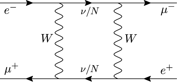
    The models with right-handed Majorana neutrinos are considered to induce the Mu-to-Mu¯\overline{\text{Mu}} transition, which will be studied mainly in Sections 4, 7.2 and 7.3. The transition operators can be generated by box loop diagrams (e.g., Fig.1 (right) and Fig.12 (right)).

  2. 2.

    (Δ​Le,Δ​Lμ)=(±2,0)(\Delta L_{e},\Delta L_{\mu})=(\pm 2,0) and (Δ​Le,Δ​Lμ)=(0,±2)(\Delta L_{e},\Delta L_{\mu})=(0,\pm 2)

    Interaction terms violate the flavor numbers separately.

    The mediators have the lepton number to be 2, and they are called dilepton bosons. The mediators have doubly electric charges. The dilepton doubly charged scalars will be studied in Sections 5, 6, and 7.1, and dilepton gauge boson will be considered in Section 10. The transition operators can be generated by tree diagrams (e.g., Fig.3 and Fig.16).

  3. 3.

    Δ​Le=−Δ​Lμ=±1\Delta L_{e}=-\Delta L_{\mu}=\pm 1

    Interaction terms violate both flavor numbers.

    The mediators are neutral bosons. The neutral scalars are considered in Sections 8 and 9.1, and neutral gauge bosons are studied in Section 11. The transition operators can be generated by tree diagram (e.g., Fig.15 and Fig.17).

    We remark that this mediator should not couple with quarks to generate the Mu-to-Mu¯\overline{\text{Mu}} transition to avoid the μ\mu – ee conversion in nuclei induced at the tree level.

  4. 4.

    (Δ​Le,Δ​Lμ)=(±1,0)(\Delta L_{e},\Delta L_{\mu})=(\pm 1,0) and (Δ​Le,Δ​Lμ)=(0,±1)(\Delta L_{e},\Delta L_{\mu})=(0,\pm 1)

    The transition operators can be generated by box loop diagrams (e.g., Fig.1 (left) and Fig.12 (left)). However, the interaction can induce μ→e​γ\mu\to e\gamma and/or μ→3​e\mu\to 3e, which restricts the size of coupling constants. Then, the magnitudes of the coefficients of the transition operators become much less than the achievement of the planned experiments, as we will see in many of the models.

In the cases 1, 2, and 3, there are interactions or mass terms with Δ​Le−Δ​Lμ=±2\Delta L_{e}-\Delta L_{\mu}=\pm 2, which are even numbers. Even in those cases, the interactions with Δ​Le−Δ​Lμ=±1\Delta L_{e}-\Delta L_{\mu}=\pm 1 may be intermingled in the respective models, and then, the magnitudes of the Mu-to-Mu¯\overline{\text{Mu}} transition is bounded by μ→e​γ\mu\to e\gamma and/or μ→3​e\mu\to 3e [8, 9]:

Br⁡(μ→e​γ)<4.2×10⁻¹³,\displaystyle{\rm Br}(\mu\to e\gamma)<4.2\times 10^{-13}, (3.1)
Br⁡(μ→3​e)<1.0×10⁻¹².\displaystyle{\rm Br}(\mu\to 3e)<1.0\times 10^{-12}. (3.2)

If ZnZ_{n} discrete symmetry can be imposed to suppress the Δ​Le−Δ​Lμ=±1\Delta L_{e}-\Delta L_{\mu}=\pm 1 interactions (while the Δ​Le−Δ​Lμ=±2\Delta L_{e}-\Delta L_{\mu}=\pm 2 interactions are allowed), the Mu-to-Mu¯\overline{\text{Mu}} transition can be as large as the current experimental bound. In other words, the observation of the Mu-to-Mu¯\overline{\text{Mu}} transition in the near-future experiments implies the existence of such discrete symmetry in the lepton sector.

The new Δ​Le−Δ​Lμ=±2\Delta L_{e}-\Delta L_{\mu}=\pm 2 interactions can induce a “wrong muon decay”:

μ+→νμ+e++ν¯e,\mu^{+}\to\nu_{\mu}+e^{+}+\bar{\nu}_{e}, (3.3)

and thus the couplings and masses of the mediators are restricted by the universality of the Fermi decay constant [23]. They are also constrained by e+​e−→e+​e−e^{+}e^{-}\to e^{+}e^{-} Bhabha scattering data. The couplings can also induce muon and electron anomalous magnetic moments. The couplings and the mediator masses to induce the Mu-to-Mu¯\overline{\text{Mu}} transition which is allowed by the PSI experiment, do not conflict with those low energy data at present. Rather, the experimental results of the Mu-to-Mu¯\overline{\text{Mu}} transitions restrict them. The data from the high-luminosity LHC, ILC, and Belle II will cooperate with the near-future Mu-to-Mu¯\overline{\text{Mu}} transition experiments.

4 Heavy Majorana neutrinos

The simplest neutrino model to acquire the Mu-to-Mu¯\overline{\text{Mu}} transition may be the models with TeV scale Majorana neutrinos, which are SM singlets. The coefficient of the transition operator from the neutrino box loop contribution is written as [24, 25, 26, 27]

G12\displaystyle\frac{G_{1}}{\sqrt{2}} =\displaystyle= GF2​MW216​π2​∑ℐ,𝒥[𝒰μL​ℐ​𝒰eL​ℐ∗​𝒰μL​𝒥​𝒰eL​𝒥∗​E0​(xℐ,x𝒥)+(𝒰μL​ℐ)2​(𝒰eL​𝒥∗)2​E1​(xℐ,x𝒥)]\displaystyle\frac{G_{F}^{2}M_{W}^{2}}{16\pi^{2}}\sum_{\cal I,J}\left[{\cal U}_{\mu_{L}{\cal I}}{\cal U}^{*}_{e_{L}{\cal I}}{\cal U}_{\mu_{L}{\cal J}}{\cal U}^{*}_{e_{L}{\cal J}}E_{0}(x_{\cal I},x_{\cal J})+({\cal U}_{\mu_{L}{\cal I}})^{2}({\cal U}^{*}_{e_{L}{\cal J}})^{2}E_{1}(x_{\cal I},x_{\cal J})\right] (4.1)
≃\displaystyle\simeq GF2​MW216​π2​∑I,J[Xμ​I​Xe​I∗​Xμ​J​Xe​J∗​E~0​(xI,xJ)+(Xμ​I)2​(Xe​J∗)2​E1​(xI,xJ)],\displaystyle\frac{G_{F}^{2}M_{W}^{2}}{16\pi^{2}}\sum_{I,J}\left[X_{\mu{I}}X^{*}_{e{I}}X_{\mu{J}}{X}^{*}_{e{J}}\tilde{E}_{0}(x_{I},x_{J})+(X_{\mu{I}})^{2}(X^{*}_{e{J}})^{2}E_{1}(x_{I},x_{J})\right],

where

xℐ=Mℐ2MW2,x_{\cal I}=\frac{M_{\cal I}^{2}}{M_{W}^{2}}, (4.2)

and see Appendix C and D for the neutrino mixing matrix 𝒰\cal U and the loop functions E0E_{0} and E1E_{1}. The E0E_{0} term comes from box diagrams such as Fig.1 (left), and E1E_{1} term comes from diagrams such as Fig.1 (right). We ignore the light neutrino masses xi=mi2/MW2≃0x_{i}=m_{i}^{2}/M_{W}^{2}\simeq 0, and one can rewrite the first line into the second line by using the unitary relation of the mixing matrix,

∑ℐ𝒰μL​ℐ​𝒰eL​ℐ∗=∑iUμ​i​Ue​i∗+∑IXμ​I​Xe​I∗=0,\sum_{\cal I}{\cal U}_{\mu_{L}{\cal I}}{\cal U}^{*}_{e_{L}{\cal I}}=\sum_{i}U_{\mu i}U^{*}_{ei}+\sum_{I}X_{\mu I}X^{*}_{eI}=0, (4.3)

and

E~0​(x,y)=E0​(x,y)−E0​(x,0)−E0​(0,y)+E0​(0,0)=E0​(x,y).\tilde{E}_{0}(x,y)=E_{0}(x,y)-E_{0}(x,0)-E_{0}(0,y)+E_{0}(0,0)=E_{0}(x,y). (4.4)
Refer to caption
Refer to caption
Figure 1: The box loop diagrams to generate the transition operator Q1Q_{1}. There are two types of contribution: the momentum parts (p/p\!\!\!/) of the numerators of neutrino propagators are picked (left), and the mass parts of the propagators are picked (right). The lepton flavors are changed at the vertices in the left diagram, while the lepton numbers are violated in the neutrino masses in the right diagram.

We enumerate the necessary facts to evaluate the loop contribution.

  1. 1.

    The mixings are bounded by electroweak precision data model-independently [28, 29]

    |Xe​I|2,|Xμ​I|2<∼0.003,|X_{eI}|^{2},|X_{\mu I}|^{2}\mathrel{\mathchoice{\lower 2.58334pt\vbox{\halign{$\m@th\displaystyle\hfil#\hfil$\cr<\crcr\sim\crcr}}}{\lower 2.58334pt\vbox{\halign{$\m@th\textstyle\hfil#\hfil$\cr<\crcr\sim\crcr}}}{\lower 2.58334pt\vbox{\halign{$\m@th\scriptstyle\hfil#\hfil$\cr<\crcr\sim\crcr}}}{\lower 2.58334pt\vbox{\halign{$\m@th\scriptscriptstyle\hfil#\hfil$\cr<\crcr\sim\crcr}}}}0.003, (4.5)

    individually (supposing only one of MIM_{I} is in the TeV scale).

  2. 2.

    The product of |Xe​I​Xμ​I||X_{eI}X_{\mu I}| is bounded by LFV processes, especially μ→e​γ\mu\to e\gamma.

    The μR→eL​γ\mu_{R}\to e_{L}\gamma decay amplitude is given as

    AR\displaystyle A_{R} =\displaystyle= e​mμ16​π2​GF2​(∑iUμ​i​Ue​i∗​F​(xi)+∑IXμ​I​Xe​I∗​F​(xI))\displaystyle\frac{em_{\mu}}{16\pi^{2}}\frac{G_{F}}{\sqrt{2}}\left(\sum_{i}U_{\mu i}U_{ei}^{*}F(x_{i})+\sum_{I}X_{\mu I}X_{eI}^{*}F(x_{I})\right) (4.6)
    =\displaystyle= e​mμ16​π2​GF2​∑IXμ​I​Xe​I∗​F~​(xI),\displaystyle\frac{em_{\mu}}{16\pi^{2}}\frac{G_{F}}{\sqrt{2}}\sum_{I}X_{\mu I}X_{eI}^{*}\tilde{F}(x_{I}),

    where

    F~​(x)=F⁡(x)−F⁡(0)=−x⁡(1−6​x+3​x2+2​x3−6​x2​ln⁡x)(1−x)4.\tilde{F}(x)=F(x)-F(0)=-\frac{x(1-6x+3x^{2}+2x^{3}-6x^{2}\ln x)}{(1-x)^{4}}. (4.7)

    One finds22 2 The decay width in our convention of the amplitude is Γ⁡(μ→e​γ)=mμ316​π2​(|AL|2+|AR|2).\Gamma(\mu\to e\gamma)=\frac{m_{\mu}^{3}}{16\pi^{2}}(|A_{L}|^{2}+|A_{R}|^{2}). (4.8) The branching ratio can be written as Br⁡(μ→e​γ)=3​α16​π​(|A~L|2+|A~R|2),{\rm Br}(\mu\to e\gamma)=\frac{3\alpha}{16\pi}(|\tilde{A}_{L}|^{2}+|\tilde{A}_{R}|^{2}), (4.9) where the dimensionless amplitude A~L,R\tilde{A}_{L,R} is defined by AL,R=e​mμ16​π2​GF​A~L,R.A_{L,R}=\frac{em_{\mu}}{16\pi^{2}}G_{F}\tilde{A}_{L,R}. (4.10)

    Br⁡(μ→e​γ)=3​α32​π​|∑IXμ​I​Xe​I∗​F~​(xI)|2,{\rm Br}(\mu\to e\gamma)=\frac{3\alpha}{32\pi}\left|\sum_{I}X_{\mu I}X^{*}_{eI}\tilde{F}\left(x_{I}\right)\right|^{2}, (4.11)

    and the bound of Br(μ→e​γ)<4.2×10⁻¹³(\mu\to e\gamma)<4.2\times 10^{-13} requires

    |∑IXμ​I∗​Xe​I​F~​(xI)|<∼4.4×10⁻⁵.\left|\sum_{I}X^{*}_{\mu I}X_{eI}\tilde{F}\left(x_{I}\right)\right|\mathrel{\mathchoice{\lower 2.58334pt\vbox{\halign{$\m@th\displaystyle\hfil#\hfil$\cr<\crcr\sim\crcr}}}{\lower 2.58334pt\vbox{\halign{$\m@th\textstyle\hfil#\hfil$\cr<\crcr\sim\crcr}}}{\lower 2.58334pt\vbox{\halign{$\m@th\scriptstyle\hfil#\hfil$\cr<\crcr\sim\crcr}}}{\lower 2.58334pt\vbox{\halign{$\m@th\scriptscriptstyle\hfil#\hfil$\cr<\crcr\sim\crcr}}}}4.4\times 10^{-5}. (4.12)
  3. 3.

    In the box loop contribution of the Mu-to-Mu¯\overline{\text{Mu}} transition in Eq.(4.1), the E0E_{0} term is generated by flavor violation, and therefore, its magnitude is bounded by μ→e​γ\mu\to e\gamma. The E1E_{1} term, on the other hand, is generated by the Majorana property of heavy neutrinos even if there is no flavor violation in principle, i.e., the E1E_{1} term can be enlarged without a constraint from μ→e​γ\mu\to e\gamma, if Xe​IX_{eI} and Xμ​JX_{\mu J} (I≠JI\neq J) can become large.

  4. 4.

    One finds

    E0​(x,y)∼14​x​yx−y​ln⁡xy,E1​(x,y)∼12​x​y​y​ln⁡x−x​ln⁡yx−y,E_{0}(x,y)\sim\frac{1}{4}\frac{xy}{x-y}\ln\frac{x}{y},\qquad E_{1}(x,y)\sim\frac{1}{2}\sqrt{xy}\frac{y\ln x-x\ln y}{x-y}, (4.13)

    and

    E0​(x,x)∼14​x,E1​(x,x)∼−12​x​ln⁡x,E_{0}(x,x)\sim\frac{1}{4}x,\qquad E_{1}(x,x)\sim-\frac{1}{2}x\ln x, (4.14)

    for large x,yx,y. Therefore, “if the neutrino mixings can be kept the same,” the Mu-to-Mu¯\overline{\text{Mu}} transition can be larger for heavier neutrinos. This is due to the longitudinal modes of gauge bosons in the unitary gauge (or Nambu-Goldstone bosons in the ’t Hooft-Feynman gauge).

  5. 5.

    For one generation (2×22\times 2 neutrino mass matrix), the light neutrino mass in type-I seesaw is mν=mD2/MNm_{\nu}=m_{D}^{2}/M_{N}, and the mixing is (Xα​I)2=mD2/MN2=mν/MN(X_{\alpha I})^{2}=m_{D}^{2}/M_{N}^{2}=m_{\nu}/M_{N}, and therefore, the Mu-to-Mu¯\overline{\text{Mu}} transition is tiny. For a three-generation case, there is freedom to enlarge the mixings, Xe​IX_{eI} and Xμ​IX_{\mu I}, while keeping the active neutrino masses tiny. Therefore, the E0E_{0} term can be larger than the naive expectation from the size of the light–heavy neutrino mixing in one generation. If two Xα​IX_{\alpha I}’s (say Xα​1X_{\alpha 1}, Xα​2X_{\alpha 2}) are large, the heavy neutrino masses need to be degenerate, M1=−M2M_{1}=-M_{2} and Xα​1=Xα​2X_{\alpha 1}=X_{\alpha 2} (or conventionally, M1=M2M_{1}=M_{2} and Xα​1=i​Xα​2X_{\alpha 1}=iX_{\alpha 2}), due to the freedom of the mass matrix. Such degeneracy can eliminate the E1E_{1} contribution. If there are more than three singlet neutrinos, such degeneracy can be released.

  6. 6.

    If the light–heavy neutrino mixing is enlarged, a sizable active neutrino mass can be generated by ZZ boson loop [30],

    (Mν)α​β≃α24​π​cos2⁡θW​∑IXα​I​Xβ​I​MI3MI2−MZ2​ln⁡MZ2MI2.(M_{\nu})_{\alpha\beta}\simeq\frac{\alpha_{2}}{4\pi\cos^{2}\theta_{W}}\sum_{I}X_{\alpha I}X_{\beta I}\frac{M_{I}^{3}}{M_{I}^{2}-M_{Z}^{2}}\ln\frac{M_{Z}^{2}}{M_{I}^{2}}. (4.15)

    The loop-induced neutrino mass can be canceled if the heavy neutrino masses are degenerate (M1=−M2M_{1}=-M_{2}). Therefore, the E1E_{1} contribution cannot be enlarged, unless the tree-level and loop-induced active neutrino masses are miraculously canceled. (Even if one allows such unnatural cancellation, the size of the coefficient is |G1|<∼O⁡(10−6)​GF|G_{1}|\mathrel{\mathchoice{\lower 2.58334pt\vbox{\halign{$\m@th\displaystyle\hfil#\hfil$\cr<\crcr\sim\crcr}}}{\lower 2.58334pt\vbox{\halign{$\m@th\textstyle\hfil#\hfil$\cr<\crcr\sim\crcr}}}{\lower 2.58334pt\vbox{\halign{$\m@th\scriptstyle\hfil#\hfil$\cr<\crcr\sim\crcr}}}{\lower 2.58334pt\vbox{\halign{$\m@th\scriptscriptstyle\hfil#\hfil$\cr<\crcr\sim\crcr}}}}O(10^{-6})G_{F} due to the constraints of light–heavy neutrino mixings from precision electroweak data, and near-future experiments cannot reach it.)

In total, the E0E_{0} contribution is bounded by μ→e​γ\mu\to e\gamma constraint, and the E1E_{1} contribution is bounded by the natural neutrino mass hierarchy.

Since the cancellation between the tree-level and loop-induced neutrino masses cannot be controlled by symmetry, an elaborated construction of the neutrino mass model is needed (e.g. the Dirac neutrino mass is forbidden) to enlarge the Mu-to-Mu¯\overline{\text{Mu}} transition naturally from the neutrino Majorana property, which we will see in Section 7. Here, we exhibit the Mu-to-Mu¯\overline{\text{Mu}} transition assuming the heavy neutrino mass degeneracy, which can be controlled by a flavor symmetry.

Refer to caption
Figure 2: The upper bound of |G1|/GF|G_{1}|/G_{F} as a function of the heavy neutrino mass. For the neutrino mass to be less than ∼30\sim 30 TeV, the Mu-to-Mu¯\overline{\text{Mu}} transition is bounded by the μ→e​γ\mu\to e\gamma constraint.

We assume that the right-handed neutrino mass matrix MNM_{N} is given as

MN=(00M10M30M100).M_{N}=\left(\begin{array}[]{ccc}0&0&M_{1}\\ 0&M_{3}&0\\ M_{1}&0&0\end{array}\right). (4.16)

Then, the light neutrino mass after seesaw is

−(Mν)α​β=(mD)α​1​(mD)β​3+(mD)α​3​(mD)β​1M1+(mD)α​2​(mD)β​2M3.-(M_{\nu})_{\alpha\beta}=\frac{(m_{D})_{\alpha 1}(m_{D})_{\beta 3}+(m_{D})_{\alpha 3}(m_{D})_{\beta 1}}{M_{1}}+\frac{(m_{D})_{\alpha 2}(m_{D})_{\beta 2}}{M_{3}}. (4.17)

The heavy neutrino masses are M1M_{1}, M2(=−M1)M_{2}\,(=-M_{1}), and M3M_{3}. The light–heavy neutrino mixings are approximately

Xα​1=Xα​2≃(mD)α​3M1,Xα​3≃0.X_{\alpha 1}=X_{\alpha 2}\simeq\frac{(m_{D})_{\alpha 3}}{M_{1}},\qquad X_{\alpha 3}\simeq 0. (4.18)

To obtain the proper size of light neutrino masses with sizable light–heavy neutrino mixings, (mD)α​1(m_{D})_{\alpha 1} needs to be small.

We plot the upper bound of |G1|/GF|G_{1}|/G_{F} in the above setup in Fig.2. For M1<∼30M_{1}\mathrel{\mathchoice{\lower 2.58334pt\vbox{\halign{$\m@th\displaystyle\hfil#\hfil$\cr<\crcr\sim\crcr}}}{\lower 2.58334pt\vbox{\halign{$\m@th\textstyle\hfil#\hfil$\cr<\crcr\sim\crcr}}}{\lower 2.58334pt\vbox{\halign{$\m@th\scriptstyle\hfil#\hfil$\cr<\crcr\sim\crcr}}}{\lower 2.58334pt\vbox{\halign{$\m@th\scriptscriptstyle\hfil#\hfil$\cr<\crcr\sim\crcr}}}}30 TeV, the Dirac mass (mD)α​3(m_{D})_{\alpha 3} is chosen just to satisfy the μ→e​γ\mu\to e\gamma bound. For M1>∼1M_{1}\mathrel{\mathchoice{\lower 2.58334pt\vbox{\halign{$\m@th\displaystyle\hfil#\hfil$\cr>\crcr\sim\crcr}}}{\lower 2.58334pt\vbox{\halign{$\m@th\textstyle\hfil#\hfil$\cr>\crcr\sim\crcr}}}{\lower 2.58334pt\vbox{\halign{$\m@th\scriptstyle\hfil#\hfil$\cr>\crcr\sim\crcr}}}{\lower 2.58334pt\vbox{\halign{$\m@th\scriptscriptstyle\hfil#\hfil$\cr>\crcr\sim\crcr}}}}1 TeV, the loop function F~\tilde{F} for μ→e​γ\mu\to e\gamma does not depend on M1M_{1} very much (due to the longitudinal modes of the gauge bosons in the unitary gauge), and thus the maximal value of |Xe​1​Xμ​1||X_{e1}X_{\mu 1}| does not depend on M1M_{1}. Therefore, in the region of 1​TeV<∼M1<∼301\ {\rm TeV}\mathrel{\mathchoice{\lower 2.58334pt\vbox{\halign{$\m@th\displaystyle\hfil#\hfil$\cr<\crcr\sim\crcr}}}{\lower 2.58334pt\vbox{\halign{$\m@th\textstyle\hfil#\hfil$\cr<\crcr\sim\crcr}}}{\lower 2.58334pt\vbox{\halign{$\m@th\scriptstyle\hfil#\hfil$\cr<\crcr\sim\crcr}}}{\lower 2.58334pt\vbox{\halign{$\m@th\scriptscriptstyle\hfil#\hfil$\cr<\crcr\sim\crcr}}}}M_{1}\mathrel{\mathchoice{\lower 2.58334pt\vbox{\halign{$\m@th\displaystyle\hfil#\hfil$\cr<\crcr\sim\crcr}}}{\lower 2.58334pt\vbox{\halign{$\m@th\textstyle\hfil#\hfil$\cr<\crcr\sim\crcr}}}{\lower 2.58334pt\vbox{\halign{$\m@th\scriptstyle\hfil#\hfil$\cr<\crcr\sim\crcr}}}{\lower 2.58334pt\vbox{\halign{$\m@th\scriptscriptstyle\hfil#\hfil$\cr<\crcr\sim\crcr}}}}30 TeV, the upper bound of the Mu-to-Mu¯\overline{\text{Mu}} transition behaves as |G1|∝M12|G_{1}|\propto M_{1}^{2} because of 4​E0∼M12/MW24E_{0}\sim M_{1}^{2}/M_{W}^{2} for M1≫MWM_{1}\gg M_{W}. For M1>∼30M_{1}\mathrel{\mathchoice{\lower 2.58334pt\vbox{\halign{$\m@th\displaystyle\hfil#\hfil$\cr>\crcr\sim\crcr}}}{\lower 2.58334pt\vbox{\halign{$\m@th\textstyle\hfil#\hfil$\cr>\crcr\sim\crcr}}}{\lower 2.58334pt\vbox{\halign{$\m@th\scriptstyle\hfil#\hfil$\cr>\crcr\sim\crcr}}}{\lower 2.58334pt\vbox{\halign{$\m@th\scriptscriptstyle\hfil#\hfil$\cr>\crcr\sim\crcr}}}}30 TeV, the μ→e​γ\mu\to e\gamma bound can satisfy for (mD)α​3<100(m_{D})_{\alpha 3}<100 GeV, and then, the upper bound behaves as |G1|∝1/M12|G_{1}|\propto 1/M_{1}^{2}.

5 Type-II seesaw model

The doubly charged scalar can couple with two charged leptons, and the Mu-to-Mu¯\overline{\text{Mu}} transition can be induced by the exchange of it at the tree level [31, 32] as shown in Fig.3. The doubly charged scalar which can couple to right-handed charged leptons is a S​U​(2)LSU(2)_{L} singlet with hypercharge Y=2Y=2, while a S​U​(2)LSU(2)_{L} triplet scalar with hypercharge Y=1Y=1 can couple to the left-handed lepton doublets ℓ\ell.

Refer to caption
Figure 3: The tree-level exchange of a doubly charged scalar boson Δ+⁣+\Delta^{++} to induce the Mu-to-Mu¯\overline{\text{Mu}} transition.

In the type-II seesaw model [33, 34, 35, 36], the neutrino masses are generated by a vacuum expectation value (vev) of the neutral component of the S​U​(2)LSU(2)_{L} triplet scalar:

(ΔL)a​b=(ΔL+⁣+ΔL+/2ΔL+/2ΔL0).(\Delta_{L})_{ab}=\left(\begin{array}[]{cc}\Delta_{L}^{++}&\Delta_{L}^{+}/\sqrt{2}\\ \Delta_{L}^{+}/\sqrt{2}&\Delta_{L}^{0}\end{array}\right). (5.1)

Therefore, the neutrino mass generation in the type-II seesaw model can be related to the Mu-to-Mu¯\overline{\text{Mu}} transition [37].

The Lagrangian of the type-II seesaw can be written as

−ℒ=(12κi​jL(ℓi​L)c¯ℓj​LΔL+μΔHHΔL∗+h.c.)+MΔ2|ΔL|2,-{\cal L}=\left(\frac{1}{2}\kappa^{L}_{ij}\overline{(\ell_{iL})^{c}}\ell_{jL}\Delta_{L}+\mu_{\Delta}HH\Delta_{L}^{*}+h.c.\right)+M_{\Delta}^{2}|\Delta_{L}|^{2}, (5.2)

where HH is a Higgs doublet with hypercharge Y=1/2Y=1/2, and μΔ\mu_{\Delta} is a dimensionful scalar trilinear coupling. The “ℓ​ℓ​ΔL\ell\ell\Delta_{L}” term is written down as

(ℓi​L)c¯​ℓj​L​ΔL=νi​Lc¯​νj​L​ΔL0−12​νi​Lc¯​ej​L​ΔL+−12​ei​Lc¯​νj​L​ΔL++ei​Lc¯​ej​L​ΔL+⁣+.\overline{(\ell_{iL})^{c}}\ell_{jL}\Delta_{L}=\overline{\nu^{c}_{iL}}\nu_{jL}\Delta_{L}^{0}-\frac{1}{\sqrt{2}}\overline{\nu^{c}_{iL}}e_{jL}\Delta_{L}^{+}-\frac{1}{\sqrt{2}}\overline{e^{c}_{iL}}\nu_{jL}\Delta_{L}^{+}+\overline{e^{c}_{iL}}e_{jL}\Delta_{L}^{++}. (5.3)

By integrating out ΔL\Delta_{L}, the dimension-five neutrino mass operator (so-called Weinberg operator, “ℓ​ℓ​H​H\ell\ell HH”) can be generated, which can be also interpreted to mean that the vev of ΔL0\Delta_{L}^{0} is vL≡⟨ΔL0⟩=−μΔ⟨H0⟩2/MΔ2v_{L}\equiv\langle\Delta_{L}^{0}\rangle=-\mu_{\Delta}\langle H^{0}\rangle^{2}/M_{\Delta}^{2}, and the type-II neutrino mass is

MνII=κL​vL.M_{\nu}^{\rm II}=\kappa^{L}v_{L}. (5.4)

As mentioned, the type-II seesaw Lagrangian contains the doubly charged scalar couplings to the left-handed charged leptons. We here describe it using two-component spinor convention to avoid the complication of the expressions33 3 𝖾i​𝖾j=eic¯​PL​ej=eiT​C​PL​ej.{\sf e}_{i}{\sf e}_{j}=\overline{e^{c}_{i}}P_{L}e_{j}=e_{i}^{T}CP_{L}e_{j}. (5.5) In the chiral representation, the four-component spinor can be expressed as e=(𝖾𝖾𝖼¯),ec=(𝖾𝖼𝖾¯),e¯=(𝖾c𝖾¯),ec¯=(𝖾𝖾𝖼¯).e=\left(\begin{array}[]{c}{\sf e}\\ \overline{\sf e^{c}}\end{array}\right),\quad e^{c}=\left(\begin{array}[]{c}{\sf e^{c}}\\ \overline{\sf e}\end{array}\right),\quad\bar{e}=\left(\begin{array}[]{cc}{\sf e}^{c}&\overline{\sf e}\end{array}\right),\quad\overline{e^{c}}=\left(\begin{array}[]{cc}{\sf e}&\overline{\sf e^{c}}\end{array}\right). (5.6) ,

−ℒ⊃12κLi​j𝖾i𝖾jΔL+⁣++12κL∗i​j𝖾¯𝗂𝖾¯𝗃Δ𝖫−⁣−+𝖬Δ𝟤Δ𝖫−⁣−Δ𝖫+⁣+,-{\cal L}\supset\frac{1}{2}\kappa^{L}_{ij}\,{\sf e}_{i}{\sf e}_{j}\Delta_{L}^{++}+\frac{1}{2}\kappa^{L*}_{ij}\,\overline{\sf e}_{i}\overline{\sf e}_{j}\Delta_{L}^{--}+M_{\Delta}^{2}\Delta_{L}^{--}\Delta_{L}^{++}, (5.7)

where 𝖾{\sf e} denotes the two-component spinor. Integrating out ΔL+⁣+=(ΔL−⁣−)∗\Delta_{L}^{++}=(\Delta_{L}^{--})^{*} by equation of motion, 1/2​κi​jL​𝖾i​𝖾j+MΔ2​Δ−⁣−=01/2\kappa^{L}_{ij}{\sf e}_{i}{\sf e}_{j}+M_{\Delta}^{2}\Delta^{--}=0, one obtains

−ℒ⊃−141MΔ2κi​jLκk​lL∗(𝖾i𝖾j)(𝖾¯𝗄𝖾¯𝗅).-{\cal L}\supset-\frac{1}{4}\frac{1}{M^{2}_{\Delta}}\kappa^{L}_{ij}\kappa^{L*}_{kl}({\sf e}_{i}{\sf e}_{j})(\overline{\sf e}_{k}\overline{\sf e}_{l}). (5.8)

Using

δβα​δα˙β˙=12​σβ​α˙μ​σ¯μβ˙​α,\delta_{\beta}^{\alpha}\delta^{\dot{\beta}}_{\dot{\alpha}}=\frac{1}{2}\sigma^{\mu}_{\beta\dot{\alpha}}\bar{\sigma}_{\mu}^{\dot{\beta}\alpha}, (5.9)

one finds

(𝖾i​𝖾j)​(𝖾¯𝗄​𝖾¯𝗅)=𝟣𝟤​(𝖾¯𝗅​σ¯μ​𝖾𝗂)​(𝖾¯𝗄​σ¯μ​𝖾𝗃).({\sf e}_{i}{\sf e}_{j})(\overline{\sf e}_{k}\overline{\sf e}_{l})=\frac{1}{2}(\overline{\sf e}_{l}\bar{\sigma}^{\mu}{\sf e}_{i})(\overline{\sf e}_{k}\bar{\sigma}_{\mu}{\sf e}_{j}). (5.10)

Expressing it in four-component fermion convention, we obtain

−ℒ⊃−181MΔ2κi​jLκk​lL∗(el¯γμPLei)(ek¯γμPLej),-{\cal L}\supset-\frac{1}{8}\frac{1}{M_{\Delta}^{2}}\kappa^{L}_{ij}\kappa^{L*}_{kl}(\overline{e_{l}}\gamma^{\mu}P_{L}e_{i})(\overline{e_{k}}\gamma_{\mu}P_{L}e_{j}), (5.11)

and the coefficient of the transition operator can be written as

G12=−κLe​eκL∗μ​μ32​MΔ2=−132​vL2​MΔ2​(MνII)e​e​(MνII)μ​μ∗.\frac{G_{1}}{\sqrt{2}}=-\frac{\kappa^{L}_{ee}\kappa^{L*}_{\mu\mu}}{32M_{\Delta}^{2}}=-\frac{1}{32v_{L}^{2}M_{\Delta}^{2}}(M_{\nu}^{\rm II})_{ee}(M_{\nu}^{\rm II})^{*}_{\mu\mu}. (5.12)

The four-Fermi operator Eq.(5.11) can generate LFV decays

Br⁡(la−→lb+​lc−​ld−)=12​(1+δc​d)​|κLa​bκL∗c​d4​GF​MΔ2|2×Br⁡(la−→lb−​ν​ν¯).{\rm Br}(l_{a}^{-}\to l_{b}^{+}l_{c}^{-}l_{d}^{-})=\frac{1}{2(1+\delta_{cd})}\left|\frac{\kappa^{L}_{ab}\kappa^{L*}_{cd}}{4G_{F}M_{\Delta}^{2}}\right|^{2}\times{\rm Br}(l_{a}^{-}\to l_{b}^{-}\nu\bar{\nu}). (5.13)

The μ→3​e\mu\to 3e decay process gives the most stringent constraint to the Mu-to-Mu¯\overline{\text{Mu}} transition in the model:

Br⁡(μ→3​e)<1.0×10⁻¹².{\rm Br}(\mu\to 3e)<1.0\times 10^{-12}. (5.14)

We find

|G1|GF=Br⁡(μ→3​e)​12​2​|κμ​μLκe​μL|<∼3.5×10⁻⁷​|κμ​μLκe​μL|.\frac{|G_{1}|}{G_{F}}=\sqrt{{\rm Br}(\mu\to 3e)}\frac{1}{2\sqrt{2}}\left|\frac{\kappa^{L}_{\mu\mu}}{\kappa^{L}_{e\mu}}\right|\mathrel{\mathchoice{\lower 2.58334pt\vbox{\halign{$\m@th\displaystyle\hfil#\hfil$\cr<\crcr\sim\crcr}}}{\lower 2.58334pt\vbox{\halign{$\m@th\textstyle\hfil#\hfil$\cr<\crcr\sim\crcr}}}{\lower 2.58334pt\vbox{\halign{$\m@th\scriptstyle\hfil#\hfil$\cr<\crcr\sim\crcr}}}{\lower 2.58334pt\vbox{\halign{$\m@th\scriptscriptstyle\hfil#\hfil$\cr<\crcr\sim\crcr}}}}3.5\times 10^{-7}\left|\frac{\kappa^{L}_{\mu\mu}}{\kappa^{L}_{e\mu}}\right|. (5.15)

We suppose that the type-II term dominates the active neutrino mass (e.g., there is no right-handed neutrino, or the type-I contribution is negligible for the right-handed neutrinos to be very heavy), and the type-II neutrino mass matrix is

MνII=UPMNS∗​diag​(m1​ei​α1,m2​ei​α2,m3)​UPMNS†,M_{\nu}^{\rm II}=U_{\rm PMNS}^{*}{\rm diag}(m_{1}e^{i\alpha_{1}},m_{2}e^{i\alpha_{2}},m_{3})U_{\rm PMNS}^{\dagger}, (5.16)

where UPMNSU_{\rm PMNS} is the Pontecorvo-Maki-Nakagawa-Sakata (PMNS) neutrino mixing matrix given by Particle Data Group convention [38], and mim_{i}’s are the active neutrino masses. Naively, one obtains

κe​μLκμ​μL∼O⁡(θ13,Δ​msol2/Δ​matm2),\frac{\kappa^{L}_{e\mu}}{\kappa^{L}_{\mu\mu}}\sim O\left(\theta_{13},\sqrt{{\Delta m^{2}_{\rm sol}}/{\Delta m^{2}_{\rm atm}}}\right), (5.17)

and |κe​μL/κμ​μL||\kappa^{L}_{e\mu}/\kappa^{L}_{\mu\mu}| is roughly 1010 – 2020%. Then, |G1|/GF|G_{1}|/G_{F} is smaller than O⁡(10−6)O(10^{-6}), which cannot be observed in near-future experiments. However, the observed neutrino mixings can be realized even if κe​μL→0\kappa^{L}_{e\mu}\to 0. From the viewpoints of the masses and mixings, κe​μL→0\kappa^{L}_{e\mu}\to 0 can happen if

  1. 1.

    The neutrino masses are degenerate, m1​ei​α1≃m2​ei​α2(≃m3)m_{1}e^{i\alpha_{1}}\simeq m_{2}e^{i\alpha_{2}}(\simeq m_{3}).

  2. 2.

    ∑Ue​i∗​Uμ​i∗​mi​ei​αi\sum U_{ei}^{*}U_{\mu i}^{*}m_{i}e^{i\alpha_{i}} is accidentally canceled, which can happen since θ13∼Δ​msol2/Δ​matm2\theta_{13}\sim\sqrt{{\Delta m^{2}_{\rm sol}}/{\Delta m^{2}_{\rm atm}}} and θ23,θ12∼O⁡(1)\theta_{23},\theta_{12}\sim O(1).

In the case of the degenerate solution, the transition probability is maximized (for fixed vLv_{L} and MΔM_{\Delta}), and then, the half-life of neutrinoless double beta decay can be just above the current bound (if other experimental data allow the solution).

Let us calculate the numerical upper bounds of |G1|/GF|G_{1}|/G_{F} allowed by the constraints from LFV decays [38]:

{Br⁡(τ→3​e),Br⁡(τ→3​μ)}<{2.7,2.1}×10−8,\displaystyle\{{\rm Br}(\tau\to 3e),{\rm Br}(\tau\to 3\mu)\}<\{2.7,2.1\}\times 10^{-8}, (5.18)
{Br⁡(τ−→e+​μ−​μ−),Br⁡(τ−→μ+​e−​e−)}<{1.7,1.5}×10−8.\displaystyle\{{\rm Br}(\tau^{-}\to e^{+}\mu^{-}\mu^{-}),{\rm Br}(\tau^{-}\to\mu^{+}e^{-}e^{-})\}<\{1.7,1.5\}\times 10^{-8}. (5.19)

The LFV decay bounds can give the upper bounds of the Mu-to-Mu¯\overline{\text{Mu}} transition as

|G1|GF\displaystyle\frac{|G_{1}|}{G_{F}} ≃\displaystyle\simeq Br⁡(τ→3​e)Br⁡(τ→e​ν​ν¯)​12​2​|κμ​μLκe​τL|<∼1.4×10⁻⁴​|κμ​μLκe​τL|,\displaystyle\sqrt{\frac{{\rm Br}(\tau\to 3e)}{{\rm Br}(\tau\to e\nu\bar{\nu})}}\frac{1}{2\sqrt{2}}\left|\frac{\kappa^{L}_{\mu\mu}}{\kappa^{L}_{e\tau}}\right|\mathrel{\mathchoice{\lower 2.58334pt\vbox{\halign{$\m@th\displaystyle\hfil#\hfil$\cr<\crcr\sim\crcr}}}{\lower 2.58334pt\vbox{\halign{$\m@th\textstyle\hfil#\hfil$\cr<\crcr\sim\crcr}}}{\lower 2.58334pt\vbox{\halign{$\m@th\scriptstyle\hfil#\hfil$\cr<\crcr\sim\crcr}}}{\lower 2.58334pt\vbox{\halign{$\m@th\scriptscriptstyle\hfil#\hfil$\cr<\crcr\sim\crcr}}}}1.4\times 10^{-4}\left|\frac{\kappa^{L}_{\mu\mu}}{\kappa^{L}_{e\tau}}\right|,
|G1|GF\displaystyle\frac{|G_{1}|}{G_{F}} ≃\displaystyle\simeq Br⁡(τ−→μ+​e−​e−)Br⁡(τ→μ​ν​ν¯)​12​2​|κμ​μLκμ​τL|<∼1.0×10⁻⁴​|κμ​μLκμ​τL|,\displaystyle\sqrt{\frac{{\rm Br}(\tau^{-}\to\mu^{+}e^{-}e^{-})}{{\rm Br}(\tau\to\mu\nu\bar{\nu})}}\frac{1}{2\sqrt{2}}\left|\frac{\kappa^{L}_{\mu\mu}}{\kappa^{L}_{\mu\tau}}\right|\mathrel{\mathchoice{\lower 2.58334pt\vbox{\halign{$\m@th\displaystyle\hfil#\hfil$\cr<\crcr\sim\crcr}}}{\lower 2.58334pt\vbox{\halign{$\m@th\textstyle\hfil#\hfil$\cr<\crcr\sim\crcr}}}{\lower 2.58334pt\vbox{\halign{$\m@th\scriptstyle\hfil#\hfil$\cr<\crcr\sim\crcr}}}{\lower 2.58334pt\vbox{\halign{$\m@th\scriptscriptstyle\hfil#\hfil$\cr<\crcr\sim\crcr}}}}1.0\times 10^{-4}\left|\frac{\kappa^{L}_{\mu\mu}}{\kappa^{L}_{\mu\tau}}\right|,
|G1|GF\displaystyle\frac{|G_{1}|}{G_{F}} ≃\displaystyle\simeq Br⁡(τ−→e+​μ−​μ−)Br⁡(τ→e​ν​ν¯)​12​2​|κe​eLκe​τL|<∼1.1×10⁻⁴​|κe​eLκe​τL|,\displaystyle\sqrt{\frac{{\rm Br}(\tau^{-}\to e^{+}\mu^{-}\mu^{-})}{{\rm Br}(\tau\to e\nu\bar{\nu})}}\frac{1}{2\sqrt{2}}\left|\frac{\kappa^{L}_{ee}}{\kappa^{L}_{e\tau}}\right|\mathrel{\mathchoice{\lower 2.58334pt\vbox{\halign{$\m@th\displaystyle\hfil#\hfil$\cr<\crcr\sim\crcr}}}{\lower 2.58334pt\vbox{\halign{$\m@th\textstyle\hfil#\hfil$\cr<\crcr\sim\crcr}}}{\lower 2.58334pt\vbox{\halign{$\m@th\scriptstyle\hfil#\hfil$\cr<\crcr\sim\crcr}}}{\lower 2.58334pt\vbox{\halign{$\m@th\scriptscriptstyle\hfil#\hfil$\cr<\crcr\sim\crcr}}}}1.1\times 10^{-4}\left|\frac{\kappa^{L}_{ee}}{\kappa^{L}_{e\tau}}\right|,
|G1|GF\displaystyle\frac{|G_{1}|}{G_{F}} ≃\displaystyle\simeq Br⁡(τ→3​μ)Br⁡(τ→μ​ν​ν¯)​12​2​|κe​eLκe​τL|<∼1.2×10⁻⁴​|κe​eLκe​τL|.\displaystyle\sqrt{\frac{{\rm Br}(\tau\to 3\mu)}{{\rm Br}(\tau\to\mu\nu\bar{\nu})}}\frac{1}{2\sqrt{2}}\left|\frac{\kappa^{L}_{ee}}{\kappa^{L}_{e\tau}}\right|\mathrel{\mathchoice{\lower 2.58334pt\vbox{\halign{$\m@th\displaystyle\hfil#\hfil$\cr<\crcr\sim\crcr}}}{\lower 2.58334pt\vbox{\halign{$\m@th\textstyle\hfil#\hfil$\cr<\crcr\sim\crcr}}}{\lower 2.58334pt\vbox{\halign{$\m@th\scriptstyle\hfil#\hfil$\cr<\crcr\sim\crcr}}}{\lower 2.58334pt\vbox{\halign{$\m@th\scriptscriptstyle\hfil#\hfil$\cr<\crcr\sim\crcr}}}}1.2\times 10^{-4}\left|\frac{\kappa^{L}_{ee}}{\kappa^{L}_{e\tau}}\right|.

The μ→e​γ\mu\to e\gamma (and μ\mu – ee conversion [39]) constraint can be written as44 4 Br⁡(μ→e​γ)=3​α16​π​|κLe​iκL∗μ​i3​GF​(1MΔ+⁣+2+18​MΔ+2)|2.{\rm Br}(\mu\to e\gamma)=\frac{3\alpha}{16\pi}\left|\frac{\kappa^{L}_{ei}\kappa^{L*}_{\mu i}}{3G_{F}}\left(\frac{1}{M_{\Delta^{++}}^{2}}+\frac{1}{8M_{\Delta^{+}}^{2}}\right)\right|^{2}. (5.56) The S​U​(2)LSU(2)_{L} triplet contains a single charged scalar, which contributes μ→e​γ\mu\to e\gamma.

|κLe​τκL∗μ​τ|MΔ2<∼1×10−3×1(1​TeV)2,\frac{|\kappa^{L}_{e\tau}\kappa^{L*}_{\mu\tau}|}{M_{\Delta}^{2}}\mathrel{\mathchoice{\lower 2.58334pt\vbox{\halign{$\m@th\displaystyle\hfil#\hfil$\cr<\crcr\sim\crcr}}}{\lower 2.58334pt\vbox{\halign{$\m@th\textstyle\hfil#\hfil$\cr<\crcr\sim\crcr}}}{\lower 2.58334pt\vbox{\halign{$\m@th\scriptstyle\hfil#\hfil$\cr<\crcr\sim\crcr}}}{\lower 2.58334pt\vbox{\halign{$\m@th\scriptscriptstyle\hfil#\hfil$\cr<\crcr\sim\crcr}}}}1\times 10^{-3}\times\frac{1}{(1\,{\rm TeV})^{2}}, (5.57)

which is interpreted as

|G1|GF<3.8×10⁻⁶​|κe​eL​κμ​μLκe​τL​κμ​τL|.\frac{|G_{1}|}{G_{F}}<3.8\times 10^{-6}\left|\frac{\kappa^{L}_{ee}\kappa^{L}_{\mu\mu}}{\kappa^{L}_{e\tau}\kappa^{L}_{\mu\tau}}\right|. (5.58)

We solve the equation κe​μL=0\kappa^{L}_{e\mu}=0 by m1​ei​α1m_{1}e^{i\alpha_{1}} to satisfy the severe μ→3​e\mu\to 3e bound. Eliminating m1​ei​α1m_{1}e^{i\alpha_{1}} from the equation, we obtain the neutrino mass matrix as a function of a Dirac phase δ\delta in the PMNS matrix and a Majorana phase α2\alpha_{2}. Therefore, the upper bounds of the Mu-to-Mu¯\overline{\text{Mu}} transition are obtained as shown in Fig.4. Surely, the plot in Fig.4 is symmetric under δ→−δ\delta\to-\delta and α2→−α2\alpha_{2}\to-\alpha_{2}, because of G1→G1∗G_{1}\to G_{1}^{*}. Near δ∼0,π\delta\sim 0,\pi (and α2∼0\alpha_{2}\sim 0), the degenerate solution can be obtained, and thus, the Mu-to-Mu¯\overline{\text{Mu}} transition can be largest there. In the inverted hierarchy case, m1m_{1} and m2m_{2} are degenerate by themselves, and the Mu-to-Mu¯\overline{\text{Mu}} transition can be large at all the points (if there is a solution to make κe​μL→0\kappa^{L}_{e\mu}\to 0). In the normal hierarchy case, κe​μL\kappa^{L}_{e\mu} can be canceled even without mass degeneracy. Actually, both κe​eL\kappa^{L}_{ee} and κe​μL\kappa^{L}_{e\mu} can be small to reproduce the neutrino oscillation data. Therefore, there is a band where the Mu-to-Mu¯\overline{\text{Mu}} transition is small in the plot.

The current strongest bound of the absolute neutrino mass is from cosmological measurement: the total neutrino mass Σ​mν<0.12\Sigma\,m_{\nu}<0.12 eV [40]. Therefore, unless there is a loophole (e.g. the neutrinos are not stable in the cosmological time scale [41]), the solution of the large degree of degeneracy is excluded and the Mu-to-Mu¯\overline{\text{Mu}} transition is bounded. In Fig.5, we show the plot of the coefficient of the Mu-to-Mu¯\overline{\text{Mu}} transition operator versus the total neutrino mass. The shown Mu-to-Mu¯\overline{\text{Mu}} transition in the plot is the upper bound from LFV as described above, generated by a mesh of δ\delta and α2\alpha_{2}. The cosmological measurements bound the Mu-to-Mu¯\overline{\text{Mu}} transition as |G1|/GF<∼O⁡(10−5)|G_{1}|/G_{F}\mathrel{\mathchoice{\lower 2.58334pt\vbox{\halign{$\m@th\displaystyle\hfil#\hfil$\cr<\crcr\sim\crcr}}}{\lower 2.58334pt\vbox{\halign{$\m@th\textstyle\hfil#\hfil$\cr<\crcr\sim\crcr}}}{\lower 2.58334pt\vbox{\halign{$\m@th\scriptstyle\hfil#\hfil$\cr<\crcr\sim\crcr}}}{\lower 2.58334pt\vbox{\halign{$\m@th\scriptscriptstyle\hfil#\hfil$\cr<\crcr\sim\crcr}}}}O(10^{-5}).

Refer to caption
Refer to caption
Figure 4: Contour plots of upper bound of log10⁡(|G1|/GF)\log_{10}(|G_{1}|/G_{F}) from LFV decays as a function of δ\delta and α2\alpha_{2} (in radian) for normal mass ordering (left) and inverted mass ordering (right). In the dark blue region, there is no solution to make κe​μL→0\kappa^{L}_{e\mu}\to 0.
Refer to caption
Refer to caption
Figure 5: The plot of |G1|/GF|G_{1}|/G_{F} allowed by LFV constraints versus the total neutrino mass for normal mass ordering (left) and inverted mass ordering (right). The vertical red line shows ∑mν=0.12\sum m_{\nu}=0.12 eV.

If we adopt the type-I seesaw contributions in addition to type-II, one can tune κe​μL\kappa^{L}_{e\mu} to be zero irrespective of the neutrino masses and mixings, and because of the many parameters, any size of the Mu-to-Mu¯\overline{\text{Mu}} transition can be fit satisfying experimental constraints in principle [37]. Supposing κe​eL∼κμ​μL∼0.3\kappa^{L}_{ee}\sim\kappa^{L}_{\mu\mu}\sim 0.3, and MΔ=600M_{\Delta}=600 GeV (the experimental bound of the doubly charged scalar mass can be found in [42, 43]), one finds

|G1|∼1×10⁻³​GF,|G_{1}|\sim 1\times 10^{-3}\,G_{F}, (5.59)

which can be soon tested by the near-future experiments.

6 Left–right model

The S​U​(3)c×S​U​(2)L×S​U​(2)R×U​(1)B−L(≡G3221)SU(3)_{c}\times SU(2)_{L}\times SU(2)_{R}\times U(1)_{B-L}(\equiv G_{3221}) gauge theory (left–right model) to induce the Mu-to-Mu¯\overline{\text{Mu}} transition [44, 45] is one of the representative models where the new experimental results in this quarter-century have brought about changes drastically. In the early 1990s, there was still room that the active neutrinos can lie around 1010 – 100100 keV. Surely, the neutrino oscillations exclude the room, and a large mixing between left-handed neutrinos and SM singlet right-handed neutrinos at such mass scale is not allowed. The meson mixing data pushes up the WRW_{R} gauge boson mass to be more than 3 TeV [46, 47]. The direct LHC data from WR+→NR​ℓR+→j​j​ℓR±​ℓR+W_{R}^{+}\to N_{R}\ell_{R}^{+}\to jj\ell_{R}^{\pm}\ell_{R}^{+} processes gives the lower bound of the WRW_{R} mass to be more than 4 TeV [48, 49, 50]. Therefore, the resume for the Mu-to-Mu¯\overline{\text{Mu}} transition in the quarter-century ago is not valid anymore.

Various experimental constraints in the left–right model, especially on the flavor physics, can be found in [51, 52]. We note that the same sign and opposite sign of the two-lepton signals from the WR+→j​j​ℓR±​ℓR+W_{R}^{+}\to jj\ell_{R}^{\pm}\ell_{R}^{+} processes can be a probe of the structure in the neutrino mass matrix, which is related to the degeneracy of the heavy neutrino masses [53].

The Dirac mass of tau neutrino is supposed to be (at least) of the order of GeV due to left–right symmetry, and thus, one needs fine-tuning to obtain the sub-eV active neutrino mass in the TeV-scale left–right model. Therefore, an extended seesaw model to generate sub-eV active neutrino mass is often considered in the TeV-scale left–right model. We employ three SM singlet fermions SiS_{i}, and consider the neutrino mass as

−ℒ=12​((νc)R¯NR¯(Sc)R¯)​ℳ​(νL(Nc)LSL)+h.c.,-{\cal L}=\frac{1}{2}\left(\begin{array}[]{ccc}\overline{(\nu^{c})_{R}}&\overline{N_{R}}&\overline{(S^{c})_{R}}\end{array}\right){\cal M}\left(\begin{array}[]{c}\nu_{L}\\ (N^{c})_{L}\\ S_{L}\end{array}\right)+h.c., (6.1)

where ℳ{\cal M} is a 9×99\times 9 mass matrix (in the basis where the charged-lepton mass matrix is diagonal),

ℳ=(0mD0mDTμNMS0MSTμS).{\cal M}=\left(\begin{array}[]{ccc}0&m_{D}&0\\ m_{D}^{T}&\mu_{N}&M_{S}\\ 0&M_{S}^{T}&\mu_{S}\end{array}\right). (6.2)

The light neutrino mass matrix is

Mνlight=mD​(MS​μS−1​MST−μN)−1​mDT≃mD​(MST)−1​μS​MS−1​mDT.M_{\nu}^{\rm light}=m_{D}(M_{S}\mu_{S}^{-1}M_{S}^{T}-\mu_{N})^{-1}m_{D}^{T}\simeq m_{D}(M_{S}^{T})^{-1}\mu_{S}M_{S}^{-1}m_{D}^{T}. (6.3)

We suppose that the Majorana mass μS\mu_{S} of the singlet SS is small, and then the active neutrino mass can be sub-eV easily even in the TeV-scale left–right model. This is sometimes called an inverse seesaw.

The Dirac mass mDm_{D} comes from the usual Dirac Yukawa coupling to Higgs bi-doublet : (𝟏,𝟐,𝟐,0)({\bf 1},{\bf 2},{\bf 2},0) under G3221G_{3221}, and MSM_{S} comes from the Φ​ℓR¯​SL\Phi\overline{\ell_{R}}S_{L} coupling with Φ:(𝟏,𝟏,𝟐,−1)\Phi:({\bf 1},{\bf 1},{\bf 2},-1) under G3221G_{3221}. The vev of Φ\Phi breaks G3221G_{3221} down to SM gauge symmetry. The Majorana mass μN\mu_{N} is generated if there is a S​U​(2)RSU(2)_{R} triplet ΔR:(𝟏,𝟏,𝟑,2)\Delta_{R}:({\bf 1},{\bf 1},{\bf 3},2) and it acquires a vev to break G3221G_{3221}. How the Mu-to-Mu¯\overline{\text{Mu}} transition is induced in the left–right model depends on with or without the S​U​(2)RSU(2)_{R} triplet. In the case without the triplet, the Mu-to-Mu¯\overline{\text{Mu}} transition is generated at the loop level, while in the case with the triplet, it can be generated at the tree level since the triplet contains the doubly charged scalar.

We parameterize55 5 Since the singlet SS does not have a reference current basis, one can parameterize the matrix MSM_{S} to be given in Eq.(6.6) without loss of generality and μS\mu_{S} to be a general 3×33\times 3 matrix.

mD=U0∗​diag​(mD1,mD2,mD3)​V0†,\displaystyle m_{D}=U_{0}^{*}\,{\rm diag}(m_{D}^{1},m_{D}^{2},m_{D}^{3})\,V_{0}^{\dagger}, (6.4)
μN=V1∗​diag​(μN1,μN2,μN3)​V1†,\displaystyle\mu_{N}=V_{1}^{*}\,{\rm diag}(\mu_{N}^{1},\mu_{N}^{2},\mu_{N}^{3})\,V_{1}^{\dagger}, (6.5)
MS=V2∗​diag​(MS1,MS2,MS3).\displaystyle M_{S}=V_{2}^{*}\,{\rm diag}(M_{S}^{1},M_{S}^{2},M_{S}^{3}). (6.6)

The convention in the diagonalization of the neutrino mass matrix is given in Appendix C. The matrix UU in the 9×99\times 9 diagonalization matrix in Eq.(C.9), which corresponds to nearly the 3×33\times 3 PMNS matrix, is a diagonalization matrix of

U0∗​mDdiag​V0†​V2​(MSdiag)−1​μS​(MSdiag)−1​V2T​V0∗​mDdiag​U0T.U_{0}^{*}m_{D}^{\rm diag}V_{0}^{\dagger}V_{2}(M_{S}^{\rm diag})^{-1}\mu_{S}(M_{S}^{\rm diag})^{-1}V_{2}^{T}V_{0}^{*}m_{D}^{\rm diag}U_{0}^{T}. (6.7)

In the left–right model, the mixings in U0U_{0} and V0V_{0} are expected to be small as CKM mixings, but the structure of MSM_{S} and μS\mu_{S} can have freedom to generate large neutrino mixings. Surely, one can also employ a S​U​(2)LSU(2)_{L} triplet and consider the type-II seesaw contribution for the active neutrino mass.

6.1 Case 1: Without S​U​(2)RSU(2)_{R} triplet

If there is no S​U​(2)RSU(2)_{R} triplet, the Mu-to-Mu¯\overline{\text{Mu}} transition is generated by a box loop diagram. In addition to the WLW_{L} – WLW_{L} loop diagram in Fig.1, we have WRW_{R} – WRW_{R} box loop contributions:

G22=GF2​MWL216​π2​gR4gL4​1z​∑I,J[Yμ​I∗​Ye​I​Yμ​J∗​Ye​J​E0​(x~I,x~J)+(Yμ​I∗)2​(Ye​J)2​E1​(x~I,x~J)],\displaystyle\frac{G_{2}}{\sqrt{2}}=\frac{G_{F}^{2}M_{W_{L}}^{2}}{16\pi^{2}}\frac{g_{R}^{4}}{g_{L}^{4}}\frac{1}{z}\sum_{I,J}\left[Y^{*}_{\mu{I}}Y_{e{I}}Y^{*}_{\mu{J}}{Y}_{e{J}}E_{0}(\tilde{x}_{I},\tilde{x}_{J})+(Y^{*}_{\mu{I}})^{2}(Y_{e{J}})^{2}E_{1}(\tilde{x}_{I},\tilde{x}_{J})\right], (6.8)

and WLW_{L} – WRW_{R} box loop contributions:

G32=−GF2​MWL28​π2gR2gL2∑I,J[Xμ​IYμ​I∗Xe​J∗Ye​JE0(xI,xJ,z)+Xμ​IYe​IXe​J∗Yμ​J∗E1(xI,xJ,z)],\displaystyle\frac{G_{3}}{\sqrt{2}}=-\frac{G_{F}^{2}M_{W_{L}}^{2}}{8\pi^{2}}\frac{g_{R}^{2}}{g_{L}^{2}}\sum_{I,J}\left[X_{\mu{I}}Y^{*}_{\mu{I}}X^{*}_{e{J}}{Y}_{e{J}}E_{0}(x_{I},x_{J},z)+X_{\mu I}Y_{e{I}}X^{*}_{eJ}Y^{*}_{\mu{J}}E_{1}(x_{I},x_{J},z)\right], (6.9)

where

x~I=MNI2MWR2,xI=MNI2MWL2,z=MWR2MWL2.\tilde{x}_{I}=\frac{M_{N_{I}}^{2}}{M_{W_{R}}^{2}},\qquad x_{I}=\frac{M_{N_{I}}^{2}}{M_{W_{L}}^{2}},\qquad z=\frac{M_{W_{R}}^{2}}{M_{W_{L}}^{2}}. (6.10)

The loop functions E0E_{0} and E1E_{1} are given in Appendix D. Strictly speaking, since there is a WLW_{L} – WRW_{R} mixing due to vevs of Higgs bi-doublets, the mass eigenstates should be quoted as their mixed states. We here neglect their mixing in the box contributions.

One can find that E1E_{1} term in G2G_{2} and E0E_{0} term in G3G_{3} correspond to the Mu-to-Mu¯\overline{\text{Mu}} transition utilized by the Majorana property of the heavy neutrinos. If there is no S​U​(2)RSU(2)_{R} triplet, the Majorana mass of the right-handed neutrino μN\mu_{N} is absent, and the heavy neutrino masses are degenerate in the setup of the inverse seesaw. Then, their contributions are canceled. Therefore, our concerns are E0E_{0} term in G2G_{2} and E1E_{1} term in G3G_{3}, which are bounded by μ→e​γ\mu\to e\gamma. The μR→eL​γ\mu_{R}\to e_{L}\gamma amplitude via WLW_{L} loop is

AR​(WL)=e​mμ16​π2​GF2​∑IXμ​I∗​Xe​I​F~​(xI),A_{R}(W_{L})=\frac{em_{\mu}}{16\pi^{2}}\frac{G_{F}}{\sqrt{2}}\sum_{I}X^{*}_{\mu I}X_{eI}\tilde{F}\left(x_{I}\right), (6.11)

where F~\tilde{F} is given in Eq.(4.7), and the μL→eR​γ\mu_{L}\to e_{R}\gamma amplitude via WRW_{R} loop is

AL​(WR)=e​mμ16​π2​GF2​gR2gL2​1z​∑IYμ​I​Ye​I∗​F~​(x~I).A_{L}(W_{R})=\frac{em_{\mu}}{16\pi^{2}}\frac{G_{F}}{\sqrt{2}}\frac{g_{R}^{2}}{g_{L}^{2}}\frac{1}{z}\sum_{I}Y_{\mu I}Y_{eI}^{*}\tilde{F}\left(\tilde{x}_{I}\right). (6.12)

Because there is a WLW_{L} – WRW_{R} mixing ξL​R\xi_{LR}, the chirality can flip at the internal line in the loop and the decay amplitudes are

AR​(WL​ – ​WR)\displaystyle A_{R}(W_{L}{\mbox{\hskip 1.0pt--\hskip 1.0pt}}W_{R}) =\displaystyle= e16​π2​ξL​R​gRgL​GF2​∑IYμ​I​Xe​I​MNI​(G⁡(xI)−1z​G​(x~I)),\displaystyle\frac{e}{16\pi^{2}}\xi_{LR}\frac{g_{R}}{g_{L}}\frac{G_{F}}{\sqrt{2}}\sum_{I}Y_{\mu I}X_{eI}M_{N_{I}}\left(G\left(x_{I}\right)-\frac{1}{z}G(\tilde{x}_{I})\right), (6.13)
AL​(WL​ – ​WR)\displaystyle A_{L}(W_{L}{\mbox{\hskip 1.0pt--\hskip 1.0pt}}W_{R}) =\displaystyle= e16​π2​ξL​R​gRgL​GF2​∑IXμ​I∗​Ye​I∗​MNI​(G⁡(xI)−1z​G​(x~I)),\displaystyle\frac{e}{16\pi^{2}}\xi_{LR}\frac{g_{R}}{g_{L}}\frac{G_{F}}{\sqrt{2}}\sum_{I}X_{\mu I}^{*}Y_{eI}^{*}M_{N_{I}}\left(G\left(x_{I}\right)-\frac{1}{z}G(\tilde{x}_{I})\right), (6.14)

where

G⁡(x)=2​(4−15​x+12​x2−x3−6​x2​ln⁡x)(1−x)3.G(x)=\frac{2(4-15x+12x^{2}-x^{3}-6x^{2}\ln x)}{(1-x)^{3}}. (6.15)

The μ→e​γ\mu\to e\gamma experimental result implies

|∑IXμ​I∗​Xe​I​F~​(xI)|,gR2gL2​1z​|∑IYμ​I​Ye​I∗​F~​(x~I)|<∼4×10⁻⁵,\left|\sum_{I}X^{*}_{\mu I}X_{eI}\tilde{F}\left(x_{I}\right)\right|,\quad\frac{g_{R}^{2}}{g_{L}^{2}}\frac{1}{z}\left|\sum_{I}Y_{\mu I}Y_{eI}^{*}\tilde{F}\left(\tilde{x}_{I}\right)\right|\mathrel{\mathchoice{\lower 2.58334pt\vbox{\halign{$\m@th\displaystyle\hfil#\hfil$\cr<\crcr\sim\crcr}}}{\lower 2.58334pt\vbox{\halign{$\m@th\textstyle\hfil#\hfil$\cr<\crcr\sim\crcr}}}{\lower 2.58334pt\vbox{\halign{$\m@th\scriptstyle\hfil#\hfil$\cr<\crcr\sim\crcr}}}{\lower 2.58334pt\vbox{\halign{$\m@th\scriptscriptstyle\hfil#\hfil$\cr<\crcr\sim\crcr}}}}4\times 10^{-5}, (6.16)

if we assume that there is no cancellation in each ALA_{L} and ARA_{R}. These two constraints restrict the Mu-to-Mu¯\overline{\text{Mu}} transition operators from WLW_{L} – WLW_{L} box and WRW_{R} – WRW_{R} box diagrams, respectively. The μ→e​γ\mu\to e\gamma bound via the WLW_{L} – WRW_{R} mixing is written as

|∑IYμ​I∗​Xe​I∗​MNI​G​(xI)|,|∑IYe​I∗​Xμ​I∗​MNI​G​(xI)|<∼40​MeV×gLgR×10−4ξL​R,\left|\sum_{I}Y_{\mu I}^{*}X_{eI}^{*}M_{N_{I}}G(x_{I})\right|,\quad\left|\sum_{I}Y_{eI}^{*}X_{\mu I}^{*}M_{N_{I}}G(x_{I})\right|\mathrel{\mathchoice{\lower 2.58334pt\vbox{\halign{$\m@th\displaystyle\hfil#\hfil$\cr<\crcr\sim\crcr}}}{\lower 2.58334pt\vbox{\halign{$\m@th\textstyle\hfil#\hfil$\cr<\crcr\sim\crcr}}}{\lower 2.58334pt\vbox{\halign{$\m@th\scriptstyle\hfil#\hfil$\cr<\crcr\sim\crcr}}}{\lower 2.58334pt\vbox{\halign{$\m@th\scriptscriptstyle\hfil#\hfil$\cr<\crcr\sim\crcr}}}}40\ {\rm MeV}\times\frac{g_{L}}{g_{R}}\times\frac{10^{-4}}{\xi_{LR}}, (6.17)

which restricts the Mu-to-Mu¯\overline{\text{Mu}} transition from the WLW_{L} – WRW_{R} box diagram. Because of

∑IXα​I∗​Yβ​I∗​MNI≃(mD)α​β,\sum_{I}X_{\alpha I}^{*}Y_{\beta I}^{*}M_{N_{I}}\simeq(m_{D})_{\alpha\beta}, (6.18)

those roughly correspond to the bounds of the e​μe\mu and μ​e\mu e elements of the Dirac neutrino mass matrix. We remark that the restriction to the Mu-to-Mu¯\overline{\text{Mu}} transition via WLW_{L} – WRW_{R} box (G3G_{3}) is severer due to the internal chirality flipping in the μ→e​γ\mu\to e\gamma diagram.

In the case without a S​U​(2)RSU(2)_{R} triplet, the Majorana mass μN=0\mu_{N}=0 at the tree level. The flavor violation of the right-handed neutrino is characterized by V2V_{2} in Eq.(6.6). To show the evaluation of the size of the Mu-to-Mu¯\overline{\text{Mu}} transition, we assume MS1≃MS2M_{S}^{1}\simeq M_{S}^{2} and (V2)13=(V2)23=0(V_{2})_{13}=(V_{2})_{23}=0 (so that MS3M_{S}^{3} does not contribute). In Fig.6, we show the upper bound of the Mu-to-Mu¯\overline{\text{Mu}} transition by the WRW_{R} box loop allowed by μ→e​γ\mu\to e\gamma constraint. We suppose gL=gRg_{L}=g_{R} in the plot. When MN(=MS1)M_{N}(=M_{S}^{1}) is fixed, the μ→e​γ\mu\to e\gamma bound to the mixing (V2)12(V_{2})_{12} is relaxed for a heavier WRW_{R}. The upper bound of the Mu-to-Mu¯\overline{\text{Mu}} transition becomes the largest for a mass of WRW_{R} just when the maximal mixing is allowed. The largest upper bound (for fixed MNM_{N}) becomes larger for larger MNM_{N} because of the behavior of the box loop function. The mass MNM_{N} comes from Φ​ℓ¯R​SL\Phi\bar{\ell}_{R}S_{L} coupling and the vev of Φ\Phi gives WRW_{R} mass. Therefore, the mass MNM_{N} should not be much larger than MWRM_{W_{R}}, and the bound of the Mu-to-Mu¯\overline{\text{Mu}} transition is estimated as |G2|/GF<∼O⁡(10−8)|G_{2}|/G_{F}\mathrel{\mathchoice{\lower 2.58334pt\vbox{\halign{$\m@th\displaystyle\hfil#\hfil$\cr<\crcr\sim\crcr}}}{\lower 2.58334pt\vbox{\halign{$\m@th\textstyle\hfil#\hfil$\cr<\crcr\sim\crcr}}}{\lower 2.58334pt\vbox{\halign{$\m@th\scriptstyle\hfil#\hfil$\cr<\crcr\sim\crcr}}}{\lower 2.58334pt\vbox{\halign{$\m@th\scriptscriptstyle\hfil#\hfil$\cr<\crcr\sim\crcr}}}}O(10^{-8}).

As we have remarked, the μ→e​γ\mu\to e\gamma bound is stronger in the case of internal chirality flipping. The Mu-to-Mu¯\overline{\text{Mu}} transition via WLW_{L} – WRW_{R} diagram is bounded to be |G3|/GF<∼O⁡(10−10)|G_{3}|/G_{F}\mathrel{\mathchoice{\lower 2.58334pt\vbox{\halign{$\m@th\displaystyle\hfil#\hfil$\cr<\crcr\sim\crcr}}}{\lower 2.58334pt\vbox{\halign{$\m@th\textstyle\hfil#\hfil$\cr<\crcr\sim\crcr}}}{\lower 2.58334pt\vbox{\halign{$\m@th\scriptstyle\hfil#\hfil$\cr<\crcr\sim\crcr}}}{\lower 2.58334pt\vbox{\halign{$\m@th\scriptscriptstyle\hfil#\hfil$\cr<\crcr\sim\crcr}}}}O(10^{-10}) as long as ξL​R>∼0.01​MWL2/MWR2\xi_{LR}\mathrel{\mathchoice{\lower 2.58334pt\vbox{\halign{$\m@th\displaystyle\hfil#\hfil$\cr>\crcr\sim\crcr}}}{\lower 2.58334pt\vbox{\halign{$\m@th\textstyle\hfil#\hfil$\cr>\crcr\sim\crcr}}}{\lower 2.58334pt\vbox{\halign{$\m@th\scriptstyle\hfil#\hfil$\cr>\crcr\sim\crcr}}}{\lower 2.58334pt\vbox{\halign{$\m@th\scriptscriptstyle\hfil#\hfil$\cr>\crcr\sim\crcr}}}}0.01M_{W_{L}}^{2}/M_{W_{R}}^{2}. We note that the WLW_{L} – WRW_{R} mixing ξL​R\xi_{LR} is proportional to MWL2/MWR2M_{W_{L}}^{2}/M_{W_{R}}^{2}, and the proportionality coefficient is determined by the ratio of the vevs of Higgs bidoublet, though we do not describe it in detail in this paper.

Refer to caption
Figure 6: The upper bound of |G2|/GF|G_{2}|/G_{F} as a function of MWRM_{W_{R}} and the heavy neutrino mass MNM_{N}.

6.2 Case 2: With S​U​(2)RSU(2)_{R} triplet

If there is S​U​(2)RSU(2)_{R} triplet Higgs to break S​U​(2)R×U​(1)B−LSU(2)_{R}\times U(1)_{B-L}, Majorana masses of the right-handed neutrinos can be generated:

−ℒ⊃12​κi​jR​ℓi​R¯​(ℓjc)L​ΔR+h.c.,-{\cal L}\supset\frac{1}{2}\kappa^{R}_{ij}\,\overline{\ell_{iR}}(\ell^{c}_{j})_{L}\Delta_{R}+h.c., (6.19)
μN=κR​⟨ΔR0⟩.\mu_{N}=\kappa^{R}\langle\Delta_{R}^{0}\rangle. (6.20)

The box loop contribution can be larger than in case 1. In this case, however, the coupling to induce the Majorana mass can generate the transition operator at the tree level, which can be surely larger than the box loop:

−ℒ⊃−181MΔ2κi​jRκk​lR∗(ei¯γμPRel)(ej¯γμPRek),-{\cal L}\supset-\frac{1}{8}\frac{1}{M_{\Delta}^{2}}\kappa^{R}_{ij}\kappa_{kl}^{R*}(\overline{e_{i}}\gamma^{\mu}P_{R}e_{l})(\overline{e_{j}}\gamma_{\mu}P_{R}e_{k}), (6.21)

and

G22=−κR∗e​eκRμ​μ32​MΔ2.\frac{G_{2}}{\sqrt{2}}=-\frac{\kappa^{R*}_{ee}\kappa^{R}_{\mu\mu}}{32M_{\Delta}^{2}}. (6.22)

When we parameterize the Majorana mass matrix as

μN=V~​diag​(μN​1,μN​2,μN​3)​V~T,\mu_{N}=\tilde{V}{\rm diag}(\mu_{N1},\mu_{N2},\mu_{N3})\tilde{V}^{T}, (6.23)

the κR\kappa^{R} matrix is written as

κα​βR=V~α​I​V~β​I​μN​I.\kappa^{R}_{\alpha\beta}=\tilde{V}_{\alpha I}\tilde{V}_{\beta I}\mu_{NI}. (6.24)

The μ→3​e\mu\to 3e bound, Br(OPENμ→3​e)<1.0×10⁻¹²\mu\to 3e)<1.0\times 10^{-12}, restricts the Mu-to-Mu¯\overline{\text{Mu}} transition similarly to the previous,

|G2|GF<∼10−6×12​2​|κμ​μRκe​μR|.\frac{|G_{2}|}{G_{F}}\mathrel{\mathchoice{\lower 2.58334pt\vbox{\halign{$\m@th\displaystyle\hfil#\hfil$\cr<\crcr\sim\crcr}}}{\lower 2.58334pt\vbox{\halign{$\m@th\textstyle\hfil#\hfil$\cr<\crcr\sim\crcr}}}{\lower 2.58334pt\vbox{\halign{$\m@th\scriptstyle\hfil#\hfil$\cr<\crcr\sim\crcr}}}{\lower 2.58334pt\vbox{\halign{$\m@th\scriptscriptstyle\hfil#\hfil$\cr<\crcr\sim\crcr}}}}10^{-6}\times\frac{1}{2\sqrt{2}}\left|\frac{\kappa^{R}_{\mu\mu}}{\kappa^{R}_{e\mu}}\right|. (6.25)

There are three ways to suppress κe​μR=V~e​1​V~μ​1​μN​1+V~e​2​V~μ​2​μN​2+V~e​3​V~μ​3​μN​3\kappa^{R}_{e\mu}=\tilde{V}_{e1}\tilde{V}_{\mu 1}\mu_{N1}+\tilde{V}_{e2}\tilde{V}_{\mu 2}\mu_{N2}+\tilde{V}_{e3}\tilde{V}_{\mu 3}\mu_{N3}.

  1. 1.

    The mixings are small: V~≃𝟏\tilde{V}\simeq{\bf 1}.

  2. 2.

    The right-handed neutrino masses are degenerate: μN​1≃μN​2\mu_{N1}\simeq\mu_{N2}.

  3. 3.

    The mixings are not small, and the masses are not degenerate, but the κe​μR\kappa^{R}_{e\mu} is accidentally canceled by the μN​3\mu_{N3} contribution.

In models with “left–right parity” (exchange symmetry ℓL↔(ℓR)c\ell_{L}\leftrightarrow(\ell_{R})^{c}), one obtains

κL=κR,\kappa^{L}=\kappa^{R}, (6.26)

and Yukawa matrices are symmetric. Therefore, in the case of the type-II dominance (μS→0\mu_{S}\to 0), κR\kappa^{R} is also related to the neutrino masses and mixings:

κR∝Mν=UPMNS∗​diag​(m1​ei​α1,m2​ei​α2,m3)​UPMNS†,\kappa^{R}\propto M_{\nu}=U_{\rm PMNS}^{*}{\rm diag}(m_{1}e^{i\alpha_{1}},m_{2}e^{i\alpha_{2}},m_{3})U_{\rm PMNS}^{\dagger}, (6.27)

and the Mu-to-Mu¯\overline{\text{Mu}} transition is estimated in parallel to the analysis in the type-II seesaw.

In general, there is no reason that V~e​2\tilde{V}_{e2} and V~μ​1\tilde{V}_{\mu 1} are small in the model construction in the left–right model. Rather, the mixing is not small in the unification scenarios, and the Mu-to-Mu¯\overline{\text{Mu}} transition is much smaller than the near-future experimental reach. If we do not go beyond the left–right symmetry, a global discrete flavor symmetry to suppress LFV can be assigned in the lepton sector and V~≃𝟏\tilde{V}\simeq{\bf 1}. (Large neutrino mixings can originate from a hidden sector with singlet fermions, where the discrete symmetry is broken.) The right-handed neutrinos (more precisely, mass eigenstates of the heavy neutrinos from NRN_{R} and SS for μN∼MS\mu_{N}\sim M_{S}), as well as WRW_{R} gauge boson, should be heavier than 44 – 55 TeV to satisfy the bound from the WR+→NR​ℓR+→j​j​ℓR±​ℓR+W_{R}^{+}\to N_{R}\ell_{R}^{+}\to jj\ell_{R}^{\pm}\ell_{R}^{+} processes at the LHC [48, 49, 50]. The doubly charged scalar mass, on the other hand, can be around 1 TeV [42, 43], and thus, the Mu-to-Mu¯\overline{\text{Mu}} transition with |G2|/GF∼10−3|G_{2}|/G_{F}\sim 10^{-3} can be obtained, which can be tested by the near-future Mu-to-Mu¯\overline{\text{Mu}} transition experiments along with the direct search at high-luminosity LHC experiment.

7 Radiative neutrino mass

There are plenty of models in which the neutrino masses are induced radiatively. The models can be roughly classified into two groups.

(1) There is no SM singlet fermion.

(2) There are SM singlet fermions, but the Dirac neutrino Yukawa coupling, N​H​ℓNH\ell, is forbidden by a discrete symmetry.

The representative model for (1) is called Zee-Babu model [10, 11, 12, 13, 54, 55, 56]. The improved version of the model has a hypercharge ±2\pm 2, S​U​(2)LSU(2)_{L} singlet scalar, which is a doubly charged scalar and can be a mediator to induce the transition operator. Neutrino masses are generated at the two-loop level. The model where the neutrino masses are induced at a three-loop level is also considered (so-called Cocktail model) [57, 58].

In the models for (2), the tree-level active neutrino masses are forbidden by discrete symmetries. Because the discrete symmetries can be exploited, the models are often discussed together with dark matter candidates [59]. As we have studied in Section 4, the enlargement of the Mu-to-Mu¯\overline{\text{Mu}} transition from the Majorana property suffers from the natural neutrino mass hierarchy due to the light–heavy neutrino mixings induced by the Dirac neutrino masses. Because of the absence of the Dirac neutrino mass, the models are also suitable to discuss the Mu-to-Mu¯\overline{\text{Mu}} transition from the Majorana property. The model for (2) has a Yukawa coupling N​η​ℓ(=N​η+​eL−N​η0​νL)N\eta\ell\,(=N\eta^{+}e_{L}-N\eta^{0}\nu_{L}) to generate the neutrino mass at the one-loop level, where the neutral component of the S​U​(2)LSU(2)_{L} doublet η\eta does not acquire a vev (η\eta is often called an inert Higgs doublet). Alternatively, the model has a N​S+​eRNS^{+}e_{R} type coupling (S+S^{+} is a hypercharge +1+1 S​U​(2)LSU(2)_{L} singlet scalar), and the neutrino masses are generated at the three-loop level [58, 60, 61]. The N​η+​eLN\eta^{+}e_{L} and N​S+​eRNS^{+}e_{R} couplings can induce the transition operators via box diagrams.

7.1 Models with doubly charged scalar

7.1.1 Zee-Babu model

In the Zee-Babu model, there are S​U​(2)LSU(2)_{L} singlet scalars, h+h^{+} and k+⁣+k^{++}, with hypercharge Y=1Y=1 and Y=2Y=2, respectively. The couplings to the leptons and the masses of the scalars are given as

−ℒ⊃(fi​jℓic¯⋅ℓjh++gi​jei¯ejck−⁣−+μh​h​kh+h+k−⁣−+h.c.)+mh2h−h++mk2k−⁣−k+⁣+,-{\cal L}\supset(f_{ij}\overline{\ell_{i}^{c}}\cdot\ell_{j}h^{+}+g_{ij}\overline{e_{i}}e_{j}^{c}k^{--}+\mu_{hhk}\,h^{+}h^{+}k^{--}+h.c.)+m_{h}^{2}h^{-}h^{+}+m_{k}^{2}k^{--}k^{++}, (7.1)

where ‘⋅\cdot’ stands for the contraction of the S​U​(2)LSU(2)_{L} doublet: A⋅B≡ϵa​b​Aa​Bb=A1​B2−A2​B1A\cdot B\equiv\epsilon_{ab}A_{a}B_{b}=A_{1}B_{2}-A_{2}B_{1}. The coupling matrix ff is antisymmetric under the flavor index, and gg is symmetric. The scalar trilinear coupling μh​h​k\mu_{hhk} violates the lepton number symmetry.

Refer to caption
Figure 7: The diagram to induce the neutrino masses in the Zee-Babu model. The symbol ⟨H⟩\langle H\rangle stands for the vev of the SM Higgs boson.

The neutrino mass can be induced by two-loop diagram in Fig.7, and the mass matrix is given as

Mν=1M0​f​Me​g​Me​fT,M_{\nu}=\frac{1}{M_{0}}fM_{e}gM_{e}f^{T}, (7.2)

where Me=diag⁡(me,mμ,mτ)M_{e}={\rm diag}(m_{e},m_{\mu},m_{\tau}),

1M0=μh​h​k48​π2​max​(mh2,mk2)​I~,\frac{1}{M_{0}}=\frac{\mu_{hhk}}{48\pi^{2}\,{\rm max}(m_{h}^{2},m_{k}^{2})}\tilde{I}, (7.3)

and the loop function is approximately given as [54, 55, 56]

I~≃{1for ​mk≪mh,1+3π2​(ln2⁡mk2mh2−1)for ​mk≫mh.\tilde{I}\simeq\left\{\begin{array}[]{cc}1&\mbox{for }\ m_{k}\ll m_{h},\\ 1+\frac{3}{\pi^{2}}\left(\ln^{2}\frac{m_{k}^{2}}{m_{h}^{2}}-1\right)&\mbox{for }\ m_{k}\gg m_{h}.\end{array}\right. (7.4)

Because ff is anti-symmetric, the neutrino mass matrix is rank 2 (i.e., m1=0m_{1}=0), and the neutrino mass matrix in the normal mass hierarchy is given by the PMNS matrix UU as

Mν=U∗​diag​(0,m2,m3)​U†=m2​u2∗​u2†+m3​u3∗​u3†,M_{\nu}=U^{*}{\rm diag}(0,m_{2},m_{3})U^{\dagger}=m_{2}u_{2}^{*}u_{2}^{\dagger}+m_{3}u_{3}^{*}u_{3}^{\dagger}, (7.5)

where mim_{i}’s are the active neutrino masses as used throughout this paper, and u2u_{2} and u3u_{3} are column vectors in U=(u1,u2,u3)U=(u_{1},u_{2},u_{3}):

u1=(c12​c13−s12​c23−ei​δ​c12​s13​s23s12​s23−ei​δ​c12​s13​c23),u2=(s12​c13c12​c23−ei​δ​s12​s13​s23−c12​s23−ei​δ​s12​s13​c23),u3=(e−i​δ​s13c13​s23c13​c23).u_{1}=\left(\begin{array}[]{c}c_{12}c_{13}\\ -s_{12}c_{23}-e^{i\delta}c_{12}s_{13}s_{23}\\ s_{12}s_{23}-e^{i\delta}c_{12}s_{13}c_{23}\end{array}\right),\ u_{2}=\left(\begin{array}[]{c}s_{12}c_{13}\\ c_{12}c_{23}-e^{i\delta}s_{12}s_{13}s_{23}\\ -c_{12}s_{23}-e^{i\delta}s_{12}s_{13}c_{23}\end{array}\right),\ u_{3}=\left(\begin{array}[]{c}e^{-i\delta}s_{13}\\ c_{13}s_{23}\\ c_{13}c_{23}\end{array}\right). (7.6)

We parameterize the anti-symmetric matrix ff as

f=(0f3−f2−f30f1f2−f10),f=\left(\begin{array}[]{ccc}0&f_{3}&-f_{2}\\ -f_{3}&0&f_{1}\\ f_{2}&-f_{1}&0\end{array}\right), (7.7)

and then,

f​f†=|vf|2​I−vf∗​vfT,ff^{\dagger}=|v_{f}|^{2}I-v_{f}^{*}v_{f}^{T}, (7.8)

where vfv_{f} is a column vector, vf=(f1,f2,f3)Tv_{f}=(f_{1},f_{2},f_{3})^{T}, and II is an identity matrix. Suppose that vfv_{f} is orthogonal to u2u_{2} and u3u_{3}, i.e., vfT​u2∗=vfT​u3∗=0v_{f}^{T}u_{2}^{*}=v_{f}^{T}u_{3}^{*}=0, which means that vf=f0​u1v_{f}=f_{0}u_{1} (f0f_{0} is a coefficient). Then, one finds

f​f†​Mν​f∗​fT=|f0|4​Mν,ff^{\dagger}M_{\nu}f^{*}f^{T}=|f_{0}|^{4}M_{\nu}, (7.9)

and

f​u1=0.fu_{1}=0. (7.10)

One can also obtain

f†​u2∗=−f0∗​u3,f†​u3∗=f0∗​u2.f^{\dagger}u_{2}^{*}=-f_{0}^{*}u_{3},\quad f^{\dagger}u_{3}^{*}=f_{0}^{*}u_{2}. (7.11)

Therefore, we find that the solution of Eq.(7.2) is

f=f0​(0Uτ​1−Uμ​1−Uτ​10Ue​1Uμ​1−Ue​10),f=f_{0}\left(\begin{array}[]{ccc}0&U_{\tau 1}&-U_{\mu 1}\\ -U_{\tau 1}&0&U_{e1}\\ U_{\mu 1}&-U_{e1}&0\end{array}\right), (7.12)

and

f02M0​Me​g​Me=m2​u3​u3T+m3​u2​u2T+a1​u1​u1T+a2​(u1​u2T+u2​u1T)+a3​(u1​u3T+u3​u1T),\frac{f_{0}^{2}}{M_{0}}M_{e}gM_{e}=m_{2}\,u_{3}u_{3}^{T}+m_{3}\,u_{2}u_{2}^{T}+a_{1}u_{1}u_{1}^{T}+a_{2}(u_{1}u_{2}^{T}+u_{2}u_{1}^{T})+a_{3}(u_{1}u_{3}^{T}+u_{3}u_{1}^{T}), (7.13)

where aia_{i}’s are arbitrary coefficients with mass dimension. Because any vectors can be given by a linear combination of uiu_{i}, there are three free complex parameters aia_{i} (and one parameter f0f_{0} in ff) in the solution.

Roughly, we obtain (supposing ai=0a_{i}=0)

f02​mμ2​gμ​μM0∼(Uμ​2)2​Δ​matm2,\frac{f_{0}^{2}m_{\mu}^{2}g_{\mu\mu}}{M_{0}}\sim(U_{\mu 2})^{2}\sqrt{\Delta m^{2}_{\rm atm}}, (7.14)

and the size of the scalar mass is estimated as

M048​π2=max⁡(mh2,mk2)μh​h​k​I~∼420​GeV×f02​gμ​μ/(Uμ​2)210−3.\frac{M_{0}}{48\pi^{2}}=\frac{{\rm max}(m_{h}^{2},m_{k}^{2})}{\mu_{hhk}\tilde{I}}\sim 420\ {\rm GeV}\times\frac{f_{0}^{2}g_{\mu\mu}/(U_{\mu 2})^{2}}{10^{-3}}. (7.15)

The coupling ff can generate μ→e​γ\mu\to e\gamma process by fe​τ​fμ​τ∗f_{e\tau}f_{\mu\tau}^{*} product:

Br⁡(μ→e​γ)=3​α16​π​|fe​τ​fμ​τ∗3​GF​mh2|2,{\rm Br}(\mu\to e\gamma)=\frac{3\alpha}{16\pi}\left|\frac{f_{e\tau}f_{\mu\tau}^{*}}{3G_{F}m_{h}^{2}}\right|^{2}, (7.16)

and therefore, the magnitude of f0f_{0} is bounded to satisfy the μ→e​γ\mu\to e\gamma experimental constraint: roughly, |f0|2<∼0.002×(mh/1​TeV)2|f_{0}|^{2}\mathrel{\mathchoice{\lower 2.58334pt\vbox{\halign{$\m@th\displaystyle\hfil#\hfil$\cr<\crcr\sim\crcr}}}{\lower 2.58334pt\vbox{\halign{$\m@th\textstyle\hfil#\hfil$\cr<\crcr\sim\crcr}}}{\lower 2.58334pt\vbox{\halign{$\m@th\scriptstyle\hfil#\hfil$\cr<\crcr\sim\crcr}}}{\lower 2.58334pt\vbox{\halign{$\m@th\scriptscriptstyle\hfil#\hfil$\cr<\crcr\sim\crcr}}}}0.002\times(m_{h}/1\ {\rm TeV})^{2}.

Since there are three free parameters aia_{i}, one can eliminate all off-diagonal elements of the coupling matrix gg to suppress the LFV three-body decays of charged leptons. In that case, however, ge​eg_{ee} becomes larger than 1 since ge​e​me2∼gμ​μ​mμ2g_{ee}m_{e}^{2}\sim g_{\mu\mu}m_{\mu}^{2}. Therefore, using one degree of freedom, we need to adjust the e​eee element of Me​g​MeM_{e}gM_{e}. Then, one of the three off-diagonal elements of gg cannot be eliminated. Because it is expected that gμ​τg_{\mu\tau} is small (gμ​τ≃gμ​μ​mμ/mτg_{\mu\tau}\simeq g_{\mu\mu}m_{\mu}/m_{\tau}), τ→3​μ\tau\to 3\mu bound can be satisfied and the other bounds of LFV processes can be satisfied by eliminating e​μe\mu and e​τe\tau elements of Me​g​MeM_{e}gM_{e} using the remaining two degrees of freedom.

Refer to caption
Refer to caption
Figure 8: The contour plots of |G2|/GF|G_{2}|/G_{F} (left), Br(τ→3​μ\tau\to 3\mu) (right) as functions of the Dirac phase δ\delta and the Majorana phase α2\alpha_{2}. The choices of parameters in the Zee-Babu model are given in the text.

In Fig.8 (left), we show the contour plot of |G2|/GF|G_{2}|/G_{F} as a function of the Dirac phase δ\delta and the Majorana phase α2\alpha_{2}, by adjusting ge​μ=ge​τ=0g_{e\mu}=g_{e\tau}=0 and ge​e=gμ​μg_{ee}=g_{\mu\mu}. The Majorana phase α2\alpha_{2} defined in the convention by Particle Data Group [38] is α2=arg⁡(m2/m3)\alpha_{2}={\rm arg}(m_{2}/m_{3}) here. We choose f02=0.002f_{0}^{2}=0.002, mk=1.2m_{k}=1.2 TeV and M0/(48​π2)=500M_{0}/(48\pi^{2})=500 GeV. In Fig.8 (right), we show Br(τ→3​μ\tau\to 3\mu). Because ge​e=gμ​μg_{ee}=g_{\mu\mu} is chosen, we obtain Br⁡(τ−→μ+​e−​e−)=Br⁡(τ→3​μ){\rm Br}(\tau^{-}\to\mu^{+}e^{-}e^{-})={\rm Br}(\tau\to 3\mu). As can be seen in Fig.8 (left), |G2|/GF|G_{2}|/G_{F} can be as large as the current experimental bound shown in Eq.(2.32).

We comment on the model-parameter dependence of the Mu-to-Mu¯\overline{\text{Mu}} transition. The coefficient of the transition operator is roughly proportional to the model parameters as

|G2|2=|ge​e​gμ​μ|8​mk2∝1f04​max⁡(mk4,mh4)μh​h​k2​mk2​ge​egμ​μ.\frac{|G_{2}|}{\sqrt{2}}=\frac{|g_{ee}g_{\mu\mu}|}{8m_{k}^{2}}\propto\frac{1}{f_{0}^{4}}\frac{{\rm max}(m_{k}^{4},m_{h}^{4})}{\mu_{hhk}^{2}m_{k}^{2}}\frac{g_{ee}}{g_{\mu\mu}}. (7.17)

Here we use Eq.(7.15) to include the constraint to reproduce the neutrino mass. The non-observation of μ→e​γ\mu\to e\gamma gives the lower bound of mh4/f04m_{h}^{4}/f_{0}^{4}. If f0f_{0} (namely ff) becomes smaller, the coupling gμ​μg_{\mu\mu} needs to be larger to reproduce the size of neutrino mass m3m_{3}, and thus, the Mu-to-Mu¯\overline{\text{Mu}} transition becomes larger. The scalar trilinear coupling μh​h​k\mu_{hhk} should not be much larger than mhm_{h} and mkm_{k} to avoid a charge breaking global minimum. Therefore, the search of the Mu-to-Mu¯\overline{\text{Mu}} transition gives a good test of the Zee-Babu model in the range of ge​e∼gμ​μg_{ee}\sim g_{\mu\mu}.

Since gμ​τg_{\mu\tau} cannot be eliminated, the τ→3​μ\tau\to 3\mu and τ−→μ+​e−​e−\tau^{-}\to\mu^{+}e^{-}e^{-} processes are generated:

{Br⁡(τ→3​μ),Br⁡(τ−→μ+​e−​e−)}=8​|G2GF|2​Br​(τ→μ​ν​ν¯)×{|gμ​τge​e|2,|gμ​τgμ​μ|2}.\{{\rm Br}(\tau\to 3\mu),{\rm Br}(\tau^{-}\to\mu^{+}e^{-}e^{-})\}=8\left|\frac{G_{2}}{G_{F}}\right|^{2}{\rm Br}(\tau\to\mu\nu\bar{\nu})\times\left\{\left|\frac{g_{\mu\tau}}{g_{ee}}\right|^{2},\left|\frac{g_{\mu\tau}}{g_{\mu\mu}}\right|^{2}\right\}. (7.18)

Because of gμ​τ≃gμ​μ​mμ/mτg_{\mu\tau}\simeq g_{\mu\mu}m_{\mu}/m_{\tau}, if the Mu-to-Mu¯\overline{\text{Mu}} transition is observed at G2/GF∼10−3G_{2}/G_{F}\sim 10^{-3}, those two LFV tau decays will be observed.

We note on the case of inverted mass hierarchy. Similarly, the rank-2 neutrino mass matrix (m3=0m_{3}=0 in this case) is given as

Mν=m1​u1∗​u1†+m2​u2∗​u2†,M_{\nu}=m_{1}u_{1}^{*}u_{1}^{\dagger}+m_{2}u_{2}^{*}u_{2}^{\dagger}, (7.19)

and the solution of Eq.(7.2) is

f=f0​(0Uτ​3−Uμ​3−Uτ​30Ue​3Uμ​3−Ue​30),f=f_{0}\left(\begin{array}[]{ccc}0&U_{\tau 3}&-U_{\mu 3}\\ -U_{\tau 3}&0&U_{e3}\\ U_{\mu 3}&-U_{e3}&0\end{array}\right), (7.20)

and

f02M0​Me​g​Me=m1​u2​u2T+m2​u1​u1T+a1​(u3​u1T+u1​u3T)+a2​(u3​u2T+u2​u3T)+a3​u3​u3T.\frac{f_{0}^{2}}{M_{0}}M_{e}gM_{e}=m_{1}\,u_{2}u_{2}^{T}+m_{2}\,u_{1}u_{1}^{T}+a_{1}(u_{3}u_{1}^{T}+u_{1}u_{3}^{T})+a_{2}(u_{3}u_{2}^{T}+u_{2}u_{3}^{T})+a_{3}u_{3}u_{3}^{T}. (7.21)

The size of gμ​μg_{\mu\mu} becomes larger than the one in the normal hierarchy to make e​eee, e​μe\mu, and e​τe\tau elements of Me​g​MeM_{e}gM_{e} to be small, under the same model parameters above. This is because Ue​3U_{e3} is small compared to the other elements, and a3a_{3} needs to be larger. Consequently, the coefficient G2G_{2} becomes larger than the current bound unless ge​eg_{ee} is made to be much smaller than gμ​μg_{\mu\mu}.

7.1.2 Cocktail model

In the Cocktail model [57], an inert Higgs doublet η\eta (which does not acquire a vev) and a hypercharge Y=1Y=1 S​U​(2)LSU(2)_{L} singlet S+S^{+} are introduced in addition to the doubly charged scalar k+⁣+k^{++}. Contrary to the Zee-Babu model, the S+S^{+} scalar does not couple to leptons directly, and the μ→e​γ\mu\to e\gamma induced by S+S^{+} loop does not bother us. The neutrino masses are generated by three-loop diagrams, which look like cocktail glass as shown in Fig.9. The mass matrix is given as

(Mν)α​β=1(16​π2)3​mα​gα​β​mβ​Fcocktailmk,(M_{\nu})_{\alpha\beta}=\frac{1}{(16\pi^{2})^{3}}m_{\alpha}g_{\alpha\beta}m_{\beta}\frac{F_{\rm cocktail}}{m_{k}}, (7.22)

where gg is a doubly charged scalar coupling to right-handed charged leptons (same as in Zee-Babu model), mαm_{\alpha} (α=e,μ,τ\alpha=e,\mu,\tau) is the charged lepton mass, mkm_{k} is a doubly charged scalar mass, and FcocktailF_{\rm cocktail} stands for a loop function containing couplings in the model.

Refer to caption
Figure 9: A diagram to induce the neutrino mass in the cocktail model. The charged scalar in the inert doublet η\eta and the S​U​(2)LSU(2)_{L} singlet scalar S+S^{+} are mixed to be H1,2+H_{1,2}^{+}. By splitting the masses of the real and imaginary parts (H0,A0H^{0},A^{0}) of the neutral scalar in η\eta, neutrino masses are generated. The symbol ⟨H⟩\langle H\rangle stands for the vev of the SM Higgs boson.

The mass scale to generate the neutrino mass matrix, Mν=U∗​diag​(m1,m2,m3)​U†M_{\nu}=U^{*}{\rm diag}(m_{1},m_{2},m_{3})U^{\dagger}, in the normal mass ordering is estimated as

mkFcocktail∼1(16​π2)3​mμ2​gμ​μm3​Uμ​32∼100​GeV×gμ​μ.\frac{m_{k}}{F_{\rm cocktail}}\sim\frac{1}{(16\pi^{2})^{3}}\frac{m_{\mu}^{2}g_{\mu\mu}}{m_{3}U_{\mu 3}^{2}}\sim 100\ {\rm GeV}\times g_{\mu\mu}. (7.23)

A large value of FcocktailF_{\rm cocktail} is needed for a realistic model to satisfy the experimental constraints. More numerical works to obtain the scale by model parameters can be found in [58]. One can immediately notice that the magnitude of e​eee and e​μe\mu elements of the neutrino mass matrix MνM_{\nu} should be much smaller than the magnitude of μ​μ\mu\mu element unless ge​eg_{ee} and ge​μg_{e\mu} are much larger than 1. Indeed, we want to make ge​μ→0g_{e\mu}\to 0 to obtain a reachable Mu-to-Mu¯\overline{\text{Mu}} transition while suppressing the μ→3​e\mu\to 3e process. If the e​eee and e​μe\mu elements of MνM_{\nu} are much smaller than the μ​μ\mu\mu element, neutrino mixings and mass ratio, and phases are constrained. The analytic relation of the neutrino mixings and mass ratio is given in Ref.[62]. In Fig.10, we show the relation between the PMNS phase δ\delta and θ23\theta_{23}. We vary θ12\theta_{12} since the relation is sensitive to it. The 3​σ3\sigma range of θ12\theta_{12} is 31.3o31.3^{\rm o} – 35.9o35.9^{\rm o} by NuFIT 5.0 [63]. Because θ23\theta_{23} is in the 3​σ3\sigma range of 40o40^{\rm o} – 52o52^{\rm o}, it predicts that δ\delta is preferred to be in the second or third quadrant roughly.

Refer to caption
Figure 10: The relation between δ\delta (radian) and θ23\theta_{23} for various θ12\theta_{12} in the case of (Mν)e​e,e​μ→0(M_{\nu})_{ee,e\mu}\to 0. We use central values for the 1-3 neutrino mixing and mass squared differences: θ13=8.57o\theta_{13}=8.57^{\rm o}, Δ​msol2=7.42×10⁻⁵\Delta m^{2}_{\rm sol}=7.42\times 10^{-5} eV2, and Δ​matm2=2.52×10⁻³\Delta m^{2}_{\rm atm}=2.52\times 10^{-3} eV2 [63].

Let us choose θ12=33.4o\theta_{12}=33.4^{\rm o}, θ13=8.57o\theta_{13}=8.57^{\rm o}, Δ​msol2=7.42×10⁻⁵\Delta m^{2}_{\rm sol}=7.42\times 10^{-5} eV2, and Δ​matm2=2.52×10⁻³\Delta m^{2}_{\rm atm}=2.52\times 10^{-3} eV2. Then, we can choose θ23=45o\theta_{23}=45^{\rm o} and δ≃π\delta\simeq\pi as a benchmark point. For ge​e=gμ​μg_{ee}=g_{\mu\mu} and ge​μ=0g_{e\mu}=0, we obtain

gα​β=(10−4.57010.0454−4.570.04540.00321)​gμ​μ.g_{\alpha\beta}=\left(\begin{array}[]{ccc}1&0&-4.57\\ 0&1&0.0454\\ -4.57&0.0454&0.00321\end{array}\right)g_{\mu\mu}. (7.24)

Because of me≪mμm_{e}\ll m_{\mu}, the numerical values of the elements are insensitive to ge​eg_{ee} to reproduce the neutrino mass matrix. It is important to notice that ge​τg_{e\tau} is large, and the Mu-to-Mu¯\overline{\text{Mu}} transition is bounded by the τ→3​e\tau\to 3e process:

|G2|GF=Br⁡(τ→3​e)Br⁡(τ→e​ν​ν¯)​12​2​|gμ​μge​τ|<3×10⁻⁵.\frac{|G_{2}|}{G_{F}}=\frac{{\rm Br}(\tau\to 3e)}{{\rm Br}(\tau\to e\nu\bar{\nu})}\frac{1}{2\sqrt{2}}\left|\frac{g_{\mu\mu}}{g_{e\tau}}\right|<3\times 10^{-5}. (7.25)

The μ→e​γ\mu\to e\gamma process also bounds the Mu-to-Mu¯\overline{\text{Mu}} transition similarly to Eq.(5.58) as

|G2|GF<3.8×10⁻⁶​|ge​e​gμ​μge​τ​gμ​τ|=1.8×10⁻⁵×|ge​egμ​μ|\frac{|G_{2}|}{G_{F}}<3.8\times 10^{-6}\left|\frac{g_{ee}g_{\mu\mu}}{g_{e\tau}g_{\mu\tau}}\right|=1.8\times 10^{-5}\times\left|\frac{g_{ee}}{g_{\mu\mu}}\right| (7.26)

in this benchmark point. We note that the Zee-Babu model has freedom to suppress ge​τg_{e\tau}, while in the cocktail model, ge​τg_{e\tau} is needed to generate θ12\theta_{12} and θ13\theta_{13} neutrino mixings. Consequently, the Mu-to-Mu¯\overline{\text{Mu}} transition is bounded in the cocktail model rather than the Zee-Babu model.

7.2 Charged Higgs contribution

Refer to caption
Figure 11: The diagram to generate the neutrino mass radiatively in the model without the Dirac neutrino masses. The symbol ⟨H⟩\langle H\rangle stands for the vev of the SM Higgs boson.

The Dirac mass is supposed to be forbidden by Z2Z_{2} symmetry. Namely, the Dirac Yukawa coupling with the SM Higgs doublet Φ\Phi is absent, but couplings with an additional inert doublet η\eta are allowed:

−ℒ⊃yα​i​ℓα¯​PR​Ni​η+12​Mi​Nic¯​Ni+h.c.-{\cal L}\supset y_{\alpha i}\overline{\ell_{\alpha}}P_{R}N_{i}\eta+\frac{1}{2}M_{i}\overline{N_{i}^{c}}N_{i}+h.c. (7.27)

If the scalar potential contains the λ5\lambda_{5} term,

V⊃λ54​(η​Φ†)2+h.c.,V\supset\frac{\lambda_{5}}{4}(\eta\Phi^{\dagger})^{2}+h.c., (7.28)

the masses (mHm_{H} and mAm_{A}) of the real and imaginary parts (H0H^{0} and A0A^{0}) of the neutral Higgs boson in the inert doublet η\eta are split:

mH2−mA2=λ5​v2,m_{H}^{2}-m_{A}^{2}=\lambda_{5}v^{2}, (7.29)

where vv is the vev of the SM Higgs boson. Then, the active neutrino masses are generated radiatively by the diagram given in Fig.11 as [59]

(Mν)α​β\displaystyle(M_{\nu})_{\alpha\beta} =\displaystyle= 116​π2​yα​i​yβ​i​Mi​(mH2mH2−Mi2​ln⁡mH2Mi2−mA2mA2−Mi2​ln⁡mA2Mi2)\displaystyle\frac{1}{16\pi^{2}}y_{\alpha i}y_{\beta i}M_{i}\left(\frac{m_{H}^{2}}{m_{H}^{2}-M_{i}^{2}}\ln\frac{m_{H}^{2}}{M_{i}^{2}}-\frac{m_{A}^{2}}{m_{A}^{2}-M_{i}^{2}}\ln\frac{m_{A}^{2}}{M_{i}^{2}}\right) (7.30)
≃\displaystyle\simeq λ5​v216​π2​yα​i​yβ​iMi​(Mi2mH2−Mi2−Mi4(mH2−Mi2)2​ln⁡mH2Mi2).\displaystyle\frac{\lambda_{5}v^{2}}{16\pi^{2}}\frac{y_{\alpha i}y_{\beta i}}{M_{i}}\left(\frac{M_{i}^{2}}{m_{H}^{2}-M_{i}^{2}}-\frac{M_{i}^{4}}{(m_{H}^{2}-M_{i}^{2})^{2}}\ln\frac{m_{H}^{2}}{M_{i}^{2}}\right).
Refer to caption
Refer to caption
Figure 12: The box loop diagrams to generate the Mu-to-Mu¯\overline{\text{Mu}} transition via the charged Higgs bosons.

The charged Higgs boson in η\eta can generate the Mu-to-Mu¯\overline{\text{Mu}} transition by the box diagrams in Fig.12:

G12=ye​i∗​yμ​i​ye​j∗​yμ​j512​π2​mη2​I2​(xi,xj)+(ye​i∗)2​(yμ​j)2256​π2​mη2​xi​xj​I1​(xi,xj),\frac{G_{1}}{\sqrt{2}}=\frac{y^{*}_{ei}y_{\mu i}y_{ej}^{*}y_{\mu j}}{512\pi^{2}m_{\eta}^{2}}I_{2}(x_{i},x_{j})+\frac{(y^{*}_{ei})^{2}(y_{\mu j})^{2}}{256\pi^{2}m_{\eta}^{2}}\sqrt{x_{i}x_{j}}\,I_{1}(x_{i},x_{j}), (7.31)

where xi=Mi2/mη2x_{i}=M_{i}^{2}/m_{\eta}^{2}, and In​(xi,xj)I_{n}(x_{i},x_{j})’s are the box loop functions given in Appendix D, and mηm_{\eta} stands for the charged Higgs boson mass. The first term is bounded by μ→e​γ\mu\to e\gamma. Let us consider whether the Mu-to-Mu¯\overline{\text{Mu}} transition from the second term can be generated avoiding the μ→e​γ\mu\to e\gamma constraint. To do that, we consider

yα​i=(ye​1000yμ​20yτ​1yτ​2yτ​3)y_{\alpha i}=\left(\begin{array}[]{ccc}y_{e1}&0&0\\ 0&y_{\mu 2}&0\\ y_{\tau 1}&y_{\tau 2}&y_{\tau 3}\end{array}\right) (7.32)

to eliminate the one-loop μ→e​γ\mu\to e\gamma amplitude via η\eta loop. (For the purpose to eliminate μ→e​γ\mu\to e\gamma, one of he​3h_{e3} and hμ​3h_{\mu 3} can be non-zero. We here suppose that both are zero to reduce the number of parameters.) Then the neutrino mass matrix is

Mν=λ5​v216​π2​(ye​12M~10ye​1​yτ​1M~10yμ​22M~2yμ​2​yτ​2M~2ye​1​yτ​1M~1yμ​2​yτ​2M~2yτ​12M~1+yτ​22M~2+yτ​32M~3),M_{\nu}=\frac{\lambda_{5}v^{2}}{16\pi^{2}}\left(\begin{array}[]{ccc}\frac{y_{e1}^{2}}{\tilde{M}_{1}}&0&\frac{y_{e1}y_{\tau 1}}{\tilde{M}_{1}}\\ 0&\frac{y_{\mu 2}^{2}}{\tilde{M}_{2}}&\frac{y_{\mu 2}y_{\tau 2}}{\tilde{M}_{2}}\\ \frac{y_{e1}y_{\tau 1}}{\tilde{M}_{1}}&\frac{y_{\mu 2}y_{\tau 2}}{\tilde{M}_{2}}&\frac{y_{\tau 1}^{2}}{\tilde{M}_{1}}+\frac{y_{\tau 2}^{2}}{\tilde{M}_{2}}+\frac{y_{\tau 3}^{2}}{\tilde{M}_{3}}\end{array}\right), (7.33)

where M~i\tilde{M}_{i} is defined to be MiM_{i} divided by a loop function so that the neutrino mass matrix is ∝yα​i​yβ​i/M^i\propto y_{\alpha i}y_{\beta i}/{\hat{M}_{i}}. The size of the coupling is estimated as

λ5​yμ​22∼10−10×M~21​TeV.\lambda_{5}y_{\mu 2}^{2}\sim 10^{-10}\times\frac{\tilde{M}_{2}}{1\,{\rm TeV}}. (7.34)

Because there are four complex parameters (up to normalization), one can fit three neutrino mixings, one mass ratio, and phases, in principle. The lightest neutrino mass m1m_{1} (with its phase) is a function of the other parameters since the e​μe\mu element is chosen to be zero.

Though the couplings have been chosen to eliminate the μ→e​γ\mu\to e\gamma process, one needs to care about τ→lα​γ\tau\to l_{\alpha}\gamma (lα=e,μl_{\alpha}=e,\mu) processes since yτ​1y_{\tau 1} and yτ​2y_{\tau 2} are needed to reproduce the neutrino mixings:

Br⁡(τ→lα​γ)=3​α16​π​|yα​i​yτ​i∗​FN​(xi)GF​mη2|2​Br​(τ→lα​ν​ν¯),{\rm Br}(\tau\to l_{\alpha}\gamma)=\frac{3\alpha}{16\pi}\left|\frac{y_{\alpha i}y_{\tau i}^{*}F_{N}(x_{i})}{G_{F}m_{\eta}^{2}}\right|^{2}{\rm Br}(\tau\to l_{\alpha}\nu\bar{\nu}), (7.35)

where

FN​(x)=1−6​x+3​x2+2​x3−6​x2​ln⁡x12​(1−x)4.F_{N}(x)=\frac{1-6x+3x^{2}+2x^{3}-6x^{2}\ln x}{12(1-x)^{4}}. (7.36)

We also need to care about muon g−2g-2 since the loop contribution gives a negative contribution to it:

Δ​aμ=−18​π2​mμ2mη2​|yμ​i|2​FN​(xi).\Delta a_{\mu}=-\frac{1}{8\pi^{2}}\frac{m_{\mu}^{2}}{m_{\eta}^{2}}|y_{\mu i}|^{2}F_{N}(x_{i}). (7.37)

We can check that the experimental bound can be satisfied even if the non-zero elements of yα​iy_{\alpha i} are O⁡(1)O(1) for mη=500m_{\eta}=500 GeV. The transition amplitude can be maximal for Mi≃mηM_{i}\simeq m_{\eta}, and we find |G1|/GF<∼O⁡(10−5)|G_{1}|/G_{F}\mathrel{\mathchoice{\lower 2.58334pt\vbox{\halign{$\m@th\displaystyle\hfil#\hfil$\cr<\crcr\sim\crcr}}}{\lower 2.58334pt\vbox{\halign{$\m@th\textstyle\hfil#\hfil$\cr<\crcr\sim\crcr}}}{\lower 2.58334pt\vbox{\halign{$\m@th\scriptstyle\hfil#\hfil$\cr<\crcr\sim\crcr}}}{\lower 2.58334pt\vbox{\halign{$\m@th\scriptscriptstyle\hfil#\hfil$\cr<\crcr\sim\crcr}}}}O(10^{-5}) for mη=500m_{\eta}=500 GeV and |yα​i|<1|y_{\alpha i}|<1.

7.3 N​S+​eRNS^{+}e_{R} coupling

We consider models with right-handed charged lepton couplings to SM singlet fermion NN:

−ℒ=hα​i​eαc¯​PR​Ni​S++12​Mi​Nic¯​Ni+MS2​S+​S−,-{\cal L}=h_{\alpha i}\overline{e^{c}_{\alpha}}P_{R}N_{i}S^{+}+\frac{1}{2}M_{i}\overline{N_{i}^{c}}N_{i}+M_{S}^{2}S^{+}S^{-}, (7.38)

where S+S^{+} is a S​U​(2)LSU(2)_{L} singlet with hypercharge Y=1Y=1. The transition operator Q2Q_{2} is generated and the coefficient is

G22=he​i​hμ​i∗​he​j​hμ​j∗512​π2​MS2​I2​(xi,xj)+(he​i)2​(hμ​j∗)2256​π2​MS2​xi​xj​I1​(xi,xj),\frac{G_{2}}{\sqrt{2}}=\frac{h_{ei}h_{\mu i}^{*}h_{ej}h_{\mu j}^{*}}{512\pi^{2}M_{S}^{2}}I_{2}(x_{i},x_{j})+\frac{(h_{ei})^{2}(h_{\mu j}^{*})^{2}}{256\pi^{2}M_{S}^{2}}\sqrt{x_{i}x_{j}}\,I_{1}(x_{i},x_{j}), (7.39)

where xi=Mi2/MS2x_{i}=M_{i}^{2}/M_{S}^{2}.

7.3.1 KNT model

Refer to caption
Figure 13: A diagram to induce the neutrino mass in the KNT model. The symbol ⟨H⟩\langle H\rangle stands for the vev of the SM Higgs boson.

In the model by Krauss-Nasri-Trodden (KNT) [60], two Y=1Y=1 S​U​(2)LSU(2)_{L} singlet scalars (we call them S1S_{1} and S2S_{2}) are introduced:

−ℒ⊃fα​β​ℓαc¯⋅ℓβ​S1++hα​j​eαc¯​PR​Nj​S2++λS​(S1+​S2−)2+h.c.-{\cal L}\supset f_{\alpha\beta}\overline{\ell^{c}_{\alpha}}\cdot\ell_{\beta}S_{1}^{+}+h_{\alpha j}\overline{e^{c}_{\alpha}}P_{R}N_{j}S^{+}_{2}+\lambda_{S}(S_{1}^{+}S_{2}^{-})^{2}+h.c. (7.40)

The neutrino mass is generated by a three-loop diagram shown in Fig.13:

(Mν)α​β=λS(16​π2)3​MS22​fα​α′​mα′​hα′​i​FKNT​(MN​i/MS2,MS1/MS2)​hβ′​i​mβ′​fβ​β′,(M_{\nu})_{\alpha\beta}=\frac{\lambda_{S}}{(16\pi^{2})^{3}M_{S_{2}}^{2}}f_{\alpha\alpha^{\prime}}m_{\alpha^{\prime}}h_{\alpha^{\prime}i}F_{\rm KNT}(M_{Ni}/M_{S_{2}},M_{S_{1}}/M_{S_{2}})h_{\beta^{\prime}i}m_{\beta^{\prime}}f_{\beta\beta^{\prime}}, (7.41)

where mα=(me,mμ,mτ)m_{\alpha}=(m_{e},m_{\mu},m_{\tau}) and FKNTF_{\rm KNT} is a loop function. The equation can be solved just similarly to the Zee-Babu model. However, the coupling hh becomes large to be in a non-perturbative region if one assumes that the observed neutrino masses are all covered by this contribution. Actually, in the Zee-Babu model in which the neutrino masses are generated by the two-loop diagram, the coupling can be O⁡(1)O(1) for several hundred GeV scalar masses, and thus, one can imagine that the coupling needs to be large to generate the neutrino mass by three-loop. This is because the anti-symmetric coupling ff needs to be small to avoid μ→e​γ\mu\to e\gamma constraint. Of course, it is possible to give up on explaining the entire neutrino mass matrix with this loop-induced contribution and assume that the neutrino masses come primarily from somewhere else. In such a situation, the hh couplings can be O⁡(1)O(1) without a contradiction with observables, and they can induce the Mu-to-Mu¯\overline{\text{Mu}} transition, potentially as large as the current bound, from the second term in Eq.(7.39).

7.3.2 AKS model

In the model by Aoki-Kanemura-Seto (AKS) [61], two Higgs doublets Φ1\Phi_{1} and Φ2\Phi_{2} to have a physical charged Higgs scalar (HH) in the loop, and one real scalar singlet η0\eta^{0} are introduced. The neutrino mass is generated by three-loop diagrams such as shown in Fig.14:

(Mν)α​β=κ2​tan2⁡β(16​π2)3​mα​mβ​hα​i​hβ​i​FAKS​(MN​i,Mη,MS,MH+)MN​i,(M_{\nu})_{\alpha\beta}=\frac{\kappa^{2}\tan^{2}\beta}{(16\pi^{2})^{3}}m_{\alpha}m_{\beta}h_{\alpha i}h_{\beta i}\frac{F_{\rm AKS}(M_{Ni},M_{\eta},M_{S},M_{H^{+}})}{M_{Ni}}, (7.42)

where κ\kappa is Φ1​Φ2​η​S\Phi_{1}\Phi_{2}\eta S coupling.

Refer to caption
Figure 14: A diagram to induce the neutrino mass in the AKS model. The symbol ⟨H⟩\langle H\rangle stands for the vev of the SM Higgs boson.

Let us consider if the observed parameters of neutrino oscillations can be reproduced with satisfying the μ→e​γ\mu\to e\gamma constraint, and see if the Mu-to-Mu¯\overline{\text{Mu}} transition can be induced by the hα​ih_{\alpha i} coupling. To do that, let us consider

hα​i=(he​1000hμ​20hτ​1hτ​2hτ​3),h_{\alpha i}=\left(\begin{array}[]{ccc}h_{e1}&0&0\\ 0&h_{\mu 2}&0\\ h_{\tau 1}&h_{\tau 2}&h_{\tau 3}\end{array}\right), (7.43)

similarly to Eq.(7.32), in order to eliminate the one-loop μ→e​γ\mu\to e\gamma amplitude via hα​ih_{\alpha i} coupling. Then the neutrino mass matrix is

Mν=κ2​tan2⁡β(16​π2)3​(me2​he​12M~10me​mτ​he​1​hτ​1M~10mμ2​hμ​22M~2mμ​mτ​hμ​2​hτ​2M~2me​mτ​he​1​hτ​1M~1mμ​mτ​hμ​2​hτ​2M~2mτ2​(hτ​12M~1+hτ​22M~2+hτ​32M~3)),M_{\nu}=\frac{\kappa^{2}\tan^{2}\beta}{(16\pi^{2})^{3}}\left(\begin{array}[]{ccc}\frac{m_{e}^{2}h_{e1}^{2}}{\tilde{M}_{1}}&0&\frac{m_{e}m_{\tau}h_{e1}h_{\tau 1}}{\tilde{M}_{1}}\\ 0&\frac{m_{\mu}^{2}h_{\mu 2}^{2}}{\tilde{M}_{2}}&\frac{m_{\mu}m_{\tau}h_{\mu 2}h_{\tau 2}}{\tilde{M}_{2}}\\ \frac{m_{e}m_{\tau}h_{e1}h_{\tau 1}}{\tilde{M}_{1}}&\frac{m_{\mu}m_{\tau}h_{\mu 2}h_{\tau 2}}{\tilde{M}_{2}}&m_{\tau}^{2}\left(\frac{h_{\tau 1}^{2}}{\tilde{M}_{1}}+\frac{h_{\tau 2}^{2}}{\tilde{M}_{2}}+\frac{h_{\tau 3}^{2}}{\tilde{M}_{3}}\right)\end{array}\right), (7.44)

where M~i=MN​i/FAKS​(MN​i)\tilde{M}_{i}=M_{Ni}/F_{\rm AKS}(M_{Ni}). We obtain the mass scale of M~2\tilde{M}_{2} as

M~2≃100​GeV×hμ​22​κ2​tan2⁡β.\tilde{M}_{2}\simeq 100\ {\rm GeV}\times h_{\mu 2}^{2}\kappa^{2}\tan^{2}\beta. (7.45)

There are two types of solutions:

  1. 1.

    Naive solution: hμ​2≪he​1∼1h_{\mu 2}\ll h_{e1}\sim 1.

    If there is no cancellation in the τ​τ\tau\tau element of MνM_{\nu}, one needs hμ​2≪he​1h_{\mu 2}\ll h_{e1} to realize the neutrino mixings. This is due to me≪mμm_{e}\ll m_{\mu}. Since hμ​2h_{\mu 2} is small, a large value of κ​tan⁡β\kappa\tan\beta is needed to obtain the proper size of the neutrino mass in this solution. Any observed neutrino mixings (within errors) and a PMNS phase δ\delta can be realized. The Mu-to-Mu¯\overline{\text{Mu}} transition is estimated as |G2|/GF<∼O⁡(10−7)|G_{2}|/G_{F}\mathrel{\mathchoice{\lower 2.58334pt\vbox{\halign{$\m@th\displaystyle\hfil#\hfil$\cr<\crcr\sim\crcr}}}{\lower 2.58334pt\vbox{\halign{$\m@th\textstyle\hfil#\hfil$\cr<\crcr\sim\crcr}}}{\lower 2.58334pt\vbox{\halign{$\m@th\scriptstyle\hfil#\hfil$\cr<\crcr\sim\crcr}}}{\lower 2.58334pt\vbox{\halign{$\m@th\scriptscriptstyle\hfil#\hfil$\cr<\crcr\sim\crcr}}}}O(10^{-7}). (If one allows a nearly non-perturbative value of he​1∼10h_{e1}\sim 10, the Mu-to-Mu¯\overline{\text{Mu}} transition can be enlarged, though.)

  2. 2.

    he​1∼hμ​2h_{e1}\sim h_{\mu 2}.

    If we allow a tuning of the τ​τ\tau\tau element of MνM_{\nu} (hτ​12/M~1+hτ​32/M~3≪hτ​22/M~2h_{\tau 1}^{2}/\tilde{M}_{1}+h_{\tau 3}^{2}/\tilde{M}_{3}\ll h_{\tau 2}^{2}/\tilde{M}_{2}) to obtain the atmospheric mixing properly, he​1∼hμ​2h_{e1}\sim h_{\mu 2} can be allowed. Both e​eee and e​μe\mu elements of MνM_{\nu} are much smaller than μ​μ\mu\mu element in this solution, and therefore, the neutrino mixings and the Dirac phase δ\delta are related as shown in Fig.10. To realize the solar neutrino mixing, one needs to enlarge hτ​1h_{\tau 1} compared to the naive solution. Since hτ​1h_{\tau 1} becomes O⁡(1)O(1), one needs to care about τ→e​γ\tau\to e\gamma process. Our estimation of the Mu-to-Mu¯\overline{\text{Mu}} transition is |G2|/GF<∼O⁡(10−6)|G_{2}|/G_{F}\mathrel{\mathchoice{\lower 2.58334pt\vbox{\halign{$\m@th\displaystyle\hfil#\hfil$\cr<\crcr\sim\crcr}}}{\lower 2.58334pt\vbox{\halign{$\m@th\textstyle\hfil#\hfil$\cr<\crcr\sim\crcr}}}{\lower 2.58334pt\vbox{\halign{$\m@th\scriptstyle\hfil#\hfil$\cr<\crcr\sim\crcr}}}{\lower 2.58334pt\vbox{\halign{$\m@th\scriptscriptstyle\hfil#\hfil$\cr<\crcr\sim\crcr}}}}O(10^{-6}).

8 Neutral scalar exchange

The Mu-to-Mu¯\overline{\text{Mu}} transition induced by the neutral scalar exchange shown in Fig.15 is considered [64].

Refer to caption
Figure 15: The tree-level exchange of a neutral scalar boson (H0H^{0}, here) to induce the Mu-to-Mu¯\overline{\text{Mu}} transition.

In general two-Higgs-doublets model, so-called type-III, the Yukawa couplings can be written as

−ℒ=(Y1)i​j​ℓi​L¯​ej​R​Φ1′+(Y2)i​j​ℓi​L¯​ej​R​Φ2′+h.c.-{\cal L}=(Y_{1})_{ij}\overline{\ell_{iL}}e_{jR}\Phi_{1}^{\prime}+(Y_{2})_{ij}\overline{\ell_{iL}}e_{jR}\Phi_{2}^{\prime}+h.c. (8.1)

and the vevs of the neutral components are ⟨Φ1′0⟩=vcosβ′\langle\Phi_{1}^{\prime 0}\rangle=v\cos\beta^{\prime}, ⟨Φ2′0⟩=vsinβ′\langle\Phi_{2}^{\prime 0}\rangle=v\sin\beta^{\prime}. Redefining the Higgs fields so that Φ1\Phi_{1} does not acquire a vev,

(Φ2Φ1)=(sin⁡β′cos⁡β′−cos⁡β′sin⁡β′)​(Φ2′Φ1′),\left(\begin{array}[]{c}\Phi_{2}\\ \Phi_{1}\end{array}\right)=\left(\begin{array}[]{cc}\sin\beta^{\prime}&\cos\beta^{\prime}\\ -\cos\beta^{\prime}&\sin\beta^{\prime}\end{array}\right)\left(\begin{array}[]{c}\Phi_{2}^{\prime}\\ \Phi_{1}^{\prime}\end{array}\right), (8.2)

we can rewrite the Yukawa interaction as

−ℒ=(Ye)i​j​ℓi​L¯​ej​R​Φ2+ρi​j​ℓi​L¯​ej​R​Φ1+h.c.,-{\cal L}=(Y_{e})_{ij}\overline{\ell_{iL}}e_{jR}\Phi_{2}+\rho_{ij}\overline{\ell_{iL}}e_{jR}\Phi_{1}+h.c., (8.3)

where

Ye=Y1sinβ′+Y2cosβ′,ρ=−Y1cosβ′+Y2sinβ′.Y_{e}=Y_{1}\sin\beta^{\prime}+Y_{2}\cos\beta^{\prime},\qquad\rho=-Y_{1}\cos\beta^{\prime}+Y_{2}\sin\beta^{\prime}. (8.4)

We can redefine sin⁡β=1\sin\beta=1. The Yukawa coupling YeY_{e} generates the charged lepton masses, and thus, we work on the flavor basis where YeY_{e} is diagonal, Ye=diag⁡(ye,yμ,yτ)Y_{e}={\rm diag}(y_{e},y_{\mu},y_{\tau}). The neutral physical Higgs interaction can be written as

−ℒ=12​(Ye​cα+ρ​sα)i​j​ei​L¯​ej​R​h+12​(Ye​sα−ρ​cα)i​j​ei​L¯​ej​R​H+i​12​ρi​j​ei​L¯​ej​R​A+h.c.,-{\cal L}=\frac{1}{\sqrt{2}}(Y_{e}c_{\alpha}+\rho s_{\alpha})_{ij}\overline{e_{iL}}e_{jR}h+\frac{1}{\sqrt{2}}(Y_{e}s_{\alpha}-\rho c_{\alpha})_{ij}\overline{e_{iL}}e_{jR}H+i\frac{1}{\sqrt{2}}\rho_{ij}\overline{e_{iL}}e_{jR}A+h.c., (8.5)

where sα=sin⁡αs_{\alpha}=\sin\alpha and cα=cos⁡αc_{\alpha}=\cos\alpha are the mixings of CP even Higgs bosons (hh and HH). Integrating out the neutral Higgs bosons, hh, HH, and AA, we extract the terms which can be the transition operators:

−ℒ=−14​(ρ212​(μL¯​eR)2+ρ12∗2​(μR¯​eL)2)​(sα2mh2+cα2mH2−1mA2)\displaystyle-{\cal L}=-\frac{1}{4}\left(\rho_{21}^{2}(\overline{\mu_{L}}e_{R})^{2}+\rho_{12}^{*2}(\overline{\mu_{R}}e_{L})^{2}\right)\left(\frac{s_{\alpha}^{2}}{m_{h}^{2}}+\frac{c_{\alpha}^{2}}{m_{H}^{2}}-\frac{1}{m_{A}^{2}}\right)
−12​ρ21​ρ12∗​(μL¯​eR)​(μR¯​eL)​(sα2mh2+cα2mH2+1mA2)+h.c.,\displaystyle-\frac{1}{2}\rho_{21}\rho_{12}^{*}(\overline{\mu_{L}}e_{R})(\overline{\mu_{R}}e_{L})\left(\frac{s_{\alpha}^{2}}{m_{h}^{2}}+\frac{c_{\alpha}^{2}}{m_{H}^{2}}+\frac{1}{m_{A}^{2}}\right)+h.c., (8.6)

and

G32\displaystyle\frac{G_{3}}{\sqrt{2}} =\displaystyle= 116​ρ21​ρ12∗​(sα2mh2+cα2mH2+1mA2),\displaystyle\frac{1}{16}\rho_{21}\rho_{12}^{*}\left(\frac{s_{\alpha}^{2}}{m_{h}^{2}}+\frac{c_{\alpha}^{2}}{m_{H}^{2}}+\frac{1}{m_{A}^{2}}\right), (8.7)
G42\displaystyle\frac{G_{4}}{\sqrt{2}} =\displaystyle= −116​ρ12∗2​(sα2mh2+cα2mH2−1mA2),\displaystyle-\frac{1}{16}\rho_{12}^{*2}\left(\frac{s_{\alpha}^{2}}{m_{h}^{2}}+\frac{c_{\alpha}^{2}}{m_{H}^{2}}-\frac{1}{m_{A}^{2}}\right), (8.8)
G52\displaystyle\frac{G_{5}}{\sqrt{2}} =\displaystyle= −116​ρ212​(sα2mh2+cα2mH2−1mA2).\displaystyle-\frac{1}{16}\rho_{21}^{2}\left(\frac{s_{\alpha}^{2}}{m_{h}^{2}}+\frac{c_{\alpha}^{2}}{m_{H}^{2}}-\frac{1}{m_{A}^{2}}\right). (8.9)

If we suppose that ρ21\rho_{21} and ρ12\rho_{12} are not zero with the other ρi​j=0\rho_{ij}=0 and sin⁡α(=cos⁡(β−α))→0\sin\alpha(=\cos(\beta-\alpha))\to 0 (alignment limit), LFV processes such as μ→e​γ\mu\to e\gamma and μ→3​e\mu\to 3e do not occur. In the limit, one obtains G4G_{4}, G5→0G_{5}\to 0. Actually, in that case, there is a global discrete Z4Z_{4} symmetry, and the charge assignments are

eL:1,eR:1,μL:3,μR:3,Φ1:2,e_{L}:1,\quad e_{R}:1,\quad\mu_{L}:3,\quad\mu_{R}:3,\quad\Phi_{1}:2, (8.10)

and the charges of the others are 0. Therefore, once the selection of ρ\rho with the alignment limit is given, LFV is not generated perturbatively. We note that the electron mass can have a loop correction from ρ12​ρ21\rho_{12}\rho_{21}. The ρ\rho terms can also induce the electron g−2g-2 and electric dipole moment (therefore, ρ12​ρ21\rho_{12}\rho_{21} should be real). The coefficient G3G_{3} can be generated satisfying the LFV constraints in the alignment limit, and the Mu-to-Mu¯\overline{\text{Mu}} transition can be around the current experimental bound.

9 SUSY

Similarly to the meson mixings, the box diagram in which superparticles propagate can generate the transition operators. Indeed, the minimally extended SUSY standard model (MSSM) contains Majorana particles known as gauginos: Bino B~\tilde{B} and Wino W~0\tilde{W}^{0}. Though the Majorana property of gauginos can be utilized to generate the Mu-to-Mu¯\overline{\text{Mu}} transition, the transition probability is bounded by the μ→e​γ\mu\to e\gamma constraint as we have seen in various models.

In the MSSM, the left-handed slepton doublet and the down-type Higgs doublet have the same quantum numbers, and thus, so-called RR-parity is introduced to distinguish them. The RR-parity is also needed to avoid rapid proton decays. If the RR-parity is broken in the lepton sector, the Mu-to-Mu¯\overline{\text{Mu}} transition can be induced at the tree-level sneutrino exchange [65], as a simple corollary of the neutral Higgs exchange (in the alignment limit) in the previous section.

In this section, we first briefly describe the previously well-known Mu-to-Mu¯\overline{\text{Mu}} transition in the RR-parity violating SUSY model, and then study the box contribution of the neutralinos and charginos in extended models.

9.1 R-parity violation

If we consider RR-parity violating terms, the transition operators can be induced at the tree level [65]. The superpotential is

W=12​λi​j​k​ℓi⋅ℓj​ekc,W=\frac{1}{2}\lambda_{ijk}\ell_{i}\cdot\ell_{j}e^{c}_{k}, (9.1)

where λj​i​k=−λi​j​k\lambda_{jik}=-\lambda_{ijk}. We introduce only λ312\lambda_{312} and λ321\lambda_{321}:

W=λ312​(ν3​e1−e3​ν1)​e2c+λ321​(ν3​e2−e3​ν2)​e1c,W=\lambda_{312}(\nu_{3}e_{1}-e_{3}\nu_{1})e^{c}_{2}+\lambda_{321}(\nu_{3}e_{2}-e_{3}\nu_{2})e^{c}_{1}, (9.2)

and Lagrangian contains

−ℒ⊃(λ312ν~τμ¯PLe+λ321ν~τe¯PLμ+h.c.)+mν~τ2|ν~τ|2,-{\cal L}\supset(\lambda_{312}\tilde{\nu}_{\tau}\overline{\mu}P_{L}e+\lambda_{321}\tilde{\nu}_{\tau}\overline{e}P_{L}\mu+h.c.)+m_{\tilde{\nu}_{\tau}}^{2}|\tilde{\nu}_{\tau}|^{2}, (9.3)

where mν~τm_{\tilde{\nu}_{\tau}} is a SUSY breaking tau-sneutrino mass. By the tau-sneutrino exchange, one obtains

G32=λ321∗​λ3128​mν~τ2.\frac{G_{3}}{\sqrt{2}}=\frac{\lambda_{321}^{*}\lambda_{312}}{8m^{2}_{\tilde{\nu}_{\tau}}}. (9.4)

The tau-neutrino mass can be generated by loop:

mντ∼λ231​λ13216​π2​A​me​mμmℓ~2,m_{\nu_{\tau}}\sim\frac{\lambda_{231}\lambda_{132}}{16\pi^{2}}\frac{Am_{e}m_{\mu}}{m_{\tilde{\ell}}^{2}}, (9.5)

where AA is a SUSY breaking trilinear scalar coupling.

9.2 Gaugino contribution

In this subsection, we describe how large Mu-to-Mu¯\overline{\text{Mu}} transition can be induced by box contribution in the MSSM with RR-parity.

Though gauginos are new Majorana particles in the MSSM, the Mu-to-Mu¯\overline{\text{Mu}} transition is strongly restricted by μ→e​γ\mu\to e\gamma constraints as we have seen several times since the gaugino interactions are (Δ​Le,Δ​Lμ)=(±1,0)(\Delta L_{e},\Delta L_{\mu})=(\pm 1,0), (0,±1)(0,\pm 1) processes. Therefore, it is not very worth describing it in detail, and we here note the rough estimation of the bound of the Mu-to-Mu¯\overline{\text{Mu}} transition from the μ→e​γ\mu\to e\gamma bound.

Using mass insertion approximation [66, 67], the μ→e​γ\mu\to e\gamma constraints of the off-diagonal elements of slepton mass matrix can be written as

g22​tan⁡β​|δ12L​L|mℓ~2​GF2<∼O⁡(10−5)\frac{g_{2}^{2}\tan\beta|\delta_{12}^{LL}|}{m_{\tilde{\ell}}^{2}G_{F}^{2}}\mathrel{\mathchoice{\lower 2.58334pt\vbox{\halign{$\m@th\displaystyle\hfil#\hfil$\cr<\crcr\sim\crcr}}}{\lower 2.58334pt\vbox{\halign{$\m@th\textstyle\hfil#\hfil$\cr<\crcr\sim\crcr}}}{\lower 2.58334pt\vbox{\halign{$\m@th\scriptstyle\hfil#\hfil$\cr<\crcr\sim\crcr}}}{\lower 2.58334pt\vbox{\halign{$\m@th\scriptscriptstyle\hfil#\hfil$\cr<\crcr\sim\crcr}}}}O(10^{-5}) (9.6)

with

δ12L​L=(Mℓ~2)12/mℓ~2.\delta_{12}^{LL}=(M_{\tilde{\ell}}^{2})_{12}/m_{\tilde{\ell}}^{2}. (9.7)

Here, Mℓ~2M_{\tilde{\ell}}^{2} is a 3×33\times 3 SUSY breaking left-handed slepton squared mass matrix, and mℓ~m_{\tilde{\ell}} is an averaged left-handed slepton mass. This L​LLL constraint mainly comes from the chargino loop diagram, and the neutralino loop can also constrain δ12R​R,L​R,R​L\delta_{12}^{RR,LR,RL} similarly. The coefficient G1G_{1} of the transition operator from Wino loop can be roughly written as

G12∼g24​(δ12L​L)2512​π2​mℓ~2​I2​(x,x)+g24​(δ12L​L)2256​π2​mℓ~2​x​I1​(x,x),\frac{G_{1}}{\sqrt{2}}\sim\frac{g_{2}^{4}(\delta^{LL}_{12})^{2}}{512\pi^{2}m_{\tilde{\ell}}^{2}}I_{2}(x,x)+\frac{g_{2}^{4}(\delta^{LL}_{12})^{2}}{256\pi^{2}m_{\tilde{\ell}}^{2}}xI_{1}(x,x), (9.8)

where x≃mW~2/mℓ~2x\simeq m_{\tilde{W}}^{2}/m_{\tilde{\ell}}^{2}. One should notice that the Mu-to-Mu¯\overline{\text{Mu}} transition needs the mass insertion twice irrespective of whether the Majorana property of Wino is used or not. Because G2b​(x,x)≃x​G1b​(x,x)<∼1G_{2}^{b}(x,x)\simeq xG_{1}^{b}(x,x)\mathrel{\mathchoice{\lower 2.58334pt\vbox{\halign{$\m@th\displaystyle\hfil#\hfil$\cr<\crcr\sim\crcr}}}{\lower 2.58334pt\vbox{\halign{$\m@th\textstyle\hfil#\hfil$\cr<\crcr\sim\crcr}}}{\lower 2.58334pt\vbox{\halign{$\m@th\scriptstyle\hfil#\hfil$\cr<\crcr\sim\crcr}}}{\lower 2.58334pt\vbox{\halign{$\m@th\scriptscriptstyle\hfil#\hfil$\cr<\crcr\sim\crcr}}}}1, it is estimated as

|G1|GF<∼O⁡(10−8)​g22​|δ12L​L|tan⁡β.\frac{|G_{1}|}{G_{F}}\mathrel{\mathchoice{\lower 2.58334pt\vbox{\halign{$\m@th\displaystyle\hfil#\hfil$\cr<\crcr\sim\crcr}}}{\lower 2.58334pt\vbox{\halign{$\m@th\textstyle\hfil#\hfil$\cr<\crcr\sim\crcr}}}{\lower 2.58334pt\vbox{\halign{$\m@th\scriptstyle\hfil#\hfil$\cr<\crcr\sim\crcr}}}{\lower 2.58334pt\vbox{\halign{$\m@th\scriptscriptstyle\hfil#\hfil$\cr<\crcr\sim\crcr}}}}O(10^{-8})\frac{g^{2}_{2}|\delta_{12}^{LL}|}{\tan\beta}. (9.9)

Therefore, the Mu-to-Mu¯\overline{\text{Mu}} transition becomes the largest if δ12L​L∼1\delta_{12}^{LL}\sim 1 is allowed for the slepton mass to be several times 10 TeV. The Bino and charged Wino box loop contribution with R​RRR, L​RLR mass insertions can be also estimated similarly. The coefficients can depend on the detail of the superparticle spectrum, but we do not survey the numerical detail since the Mu-to-Mu¯\overline{\text{Mu}} transition is tiny. The chargino and neutralino contribution of μR→eL​γ\mu_{R}\to e_{L}\gamma amplitude can be canceled, but the μ\mu – ee conversion is not simultaneously canceled, and thus, it constrains the Mu-to-Mu¯\overline{\text{Mu}} transition.

9.3 Charged Higgsino contribution

If Δ​L=±2\Delta L=\pm 2 neutrino mass can be utilized, the Mu-to-Mu¯\overline{\text{Mu}} transition can be potentially generated avoiding the μ→e​γ\mu\to e\gamma constraint. However, as we have seen, the size of neutrino mass restricts the Mu-to-Mu¯\overline{\text{Mu}} transition. This is because Dirac neutrino masses induce light–heavy neutrino mixings, and large active neutrino masses can be generated at the loop level, even if we adjust the tree-level neutrino masses to be zero. In the situation that the loop-induced mass is suppressed by a flavor symmetry, the box contribution of the Mu-to-Mu¯\overline{\text{Mu}} transition is also suppressed. In the SUSY limit, the loop-induced masses are zero due to the non-renormalization theorem. By soft terms of SUSY breaking, the neutrino masses are induced but the size of the loop-induced mass can be suppressed compared to the non-SUSY case [68]. As a result, the Dirac mass or the light–heavy neutrino mixing can be larger than the one in the non-SUSY case, and the Mu-to-Mu¯\overline{\text{Mu}} transition can be larger. Although it can be larger, it is not large enough to observe in near-future experiments. Therefore, similarly to the non-SUSY model, let us consider a model with inert Higgs doublets and Dirac mass is forbidden by discrete symmetry.

The model we now consider is the SUSY version of the model in Section 7.2. We introduce additional Higgs doublets η\eta and η′\eta^{\prime} (because of gauge anomaly, we need to introduce a pair of Higgs doubles in the SUSY model), and the Yukawa coupling to η\eta with hypercharge Y=1/2Y=1/2:

W=yα​i​η⋅ℓα​Ni=yα​i​(η+​eα−η0​να)​Ni.W=y_{\alpha i}\,\eta\cdot\ell_{\alpha}N_{i}=y_{\alpha i}(\eta^{+}e_{\alpha}-\eta^{0}\nu_{\alpha})N_{i}. (9.10)

We suppose that η0\eta^{0} does not acquire a vev and the Dirac neutrino mass is absent. In order to avoid too large neutrino masses, we introduce a discrete symmetry to forbid a η⋅Hd\eta\cdot H_{d} mass term. In the SUSY model, the so-called λ5\lambda_{5} term (η​Hd)2(\eta H_{d})^{2} is absent in the FF-term and DD-term scalar potentials in the SUSY limit, and the neutrino mass shown in Section 7.2 is not generated. Introducing the (η​Hd)2(\eta H_{d})^{2} term in the superpotential, one obtains the λ5\lambda_{5} term by Bino and Wino dressing, and the tiny neutrino masses can be generated. Alternatively, one can apply the type-II seesaw to generate the neutrino mass.

The box loop via the charged scalar η+\eta^{+} is the same as in Section 7.2. We here consider the box loop via the charged Higgsino η~+\tilde{\eta}^{+} and sneutrino N~\tilde{N}. The sneutrino masses are given as

−ℒ⊃(mN~2)i​jN~iN~j†+(12Bi​jN~iN~j+h.c.),-{\cal L}\supset(m_{\tilde{N}}^{2})_{ij}\tilde{N}_{i}\tilde{N}_{j}^{\dagger}+(\frac{1}{2}B_{ij}\tilde{N}_{i}\tilde{N}_{j}+h.c.), (9.11)

where mN~2m_{\tilde{N}}^{2} contains the SUSY breaking squared mass and Majorana mass of NN, 1/2​Mi​Ni​Ni1/2M_{i}N_{i}N_{i}, and Bi​jB_{ij}’s are the coefficients of the SUSY breaking bilinear terms. For simplicity, we assume that (mN~2)i​j(m_{\tilde{N}}^{2})_{ij} and Bi​jB_{ij} are flavor diagonal. By a field redefinition, Bi​iB_{ii} can be made to be real and positive. Then, masses of the sneutrinos for 2​Re​N~\sqrt{2}\,{\rm Re}\,\tilde{N} and 2​Im​N~\sqrt{2}\,{\rm Im}\,\tilde{N} are (mN~2)i​i±Bi​i(m_{\tilde{N}}^{2})_{ii}\pm B_{ii}. The coefficient of the Mu-to-Mu¯\overline{\text{Mu}} transition operator from the sneutrino box loop diagram is obtained as

G12\displaystyle\frac{G_{1}}{\sqrt{2}} =\displaystyle= 12048​π2​mη~2​(ye​i​yμ​i∗​ye​j​yμ​j∗​(I2​(xR​i,xR​j)+I2​(xR​i,xI​j)+I2​(xI​i,xR​j)+I2​(xI​i,xI​j))CLOSE\displaystyle\frac{1}{2048\pi^{2}m_{\tilde{\eta}}^{2}}\left(y_{ei}y_{\mu i}^{*}y_{ej}y_{\mu j}^{*}\left(I_{2}(x_{Ri},x_{Rj})+I_{2}(x_{Ri},x_{Ij})+I_{2}(x_{Ii},x_{Rj})+I_{2}(x_{Ii},x_{Ij})\right)\right. (9.12)
OPEN+(ye​i)2​(yμ​j∗)2​(I2​(xR​i,xR​j)−I2​(xR​i,xI​j)−I2​(xI​i,xR​j)+I2​(xI​i,xI​j))),\displaystyle\left.+(y_{ei})^{2}(y_{\mu j}^{*})^{2}\left(I_{2}(x_{Ri},x_{Rj})-I_{2}(x_{Ri},x_{Ij})-I_{2}(x_{Ii},x_{Rj})+I_{2}(x_{Ii},x_{Ij})\right)\right),

where

xR​i=(mN~2+B)i​imη~2,xI​i=(mN~2−B)i​imη~2.x_{Ri}=\frac{(m^{2}_{\tilde{N}}+B)_{ii}}{m^{2}_{\tilde{\eta}}},\qquad x_{Ii}=\frac{(m^{2}_{\tilde{N}}-B)_{ii}}{m^{2}_{\tilde{\eta}}}. (9.13)

We suppose that the Yukawa coupling is given in Eq.(7.32) to eliminate μ→e​γ\mu\to e\gamma. Then, the first term of G1G_{1} in Eq.(9.12) becomes zero, and the second term remains if Bi​i≠0B_{ii}\neq 0 (which reminds us the BB-term violates lepton number conservation). The Yukawa coupling can generate τ→μ⁡(e)​γ\tau\to\mu(e)\gamma:

Br⁡(τ→lα​γ)=3​α16​π​|yα​i∗​yτ​i​(FN​(xR​i)+FN​(xI​i)2​GF​mη~2−FN​(xi)GF​mη2)|2​Br​(τ→lα​ν​ν¯),{\rm Br}(\tau\to l_{\alpha}\gamma)=\frac{3\alpha}{16\pi}\left|y_{\alpha i}^{*}y_{\tau i}\left(\frac{F_{N}(x_{Ri})+F_{N}(x_{Ii})}{2G_{F}m_{\tilde{\eta}}^{2}}-\frac{F_{N}(x_{i})}{G_{F}m_{\eta}^{2}}\right)\right|^{2}{\rm Br}(\tau\to l_{\alpha}\nu\bar{\nu}), (9.14)

where xi=Mi2/mη2x_{i}=M_{i}^{2}/m_{\eta}^{2}, and the loop function FN​(x)F_{N}(x) is given in Eq.(7.36). The Mu-to-Mu¯\overline{\text{Mu}} transition can be the largest when xI​i≪1≪xR​ix_{Ii}\ll 1\ll x_{Ri}, and our estimation is |G1|/GF<∼O⁡(10−5)|G_{1}|/G_{F}\mathrel{\mathchoice{\lower 2.58334pt\vbox{\halign{$\m@th\displaystyle\hfil#\hfil$\cr<\crcr\sim\crcr}}}{\lower 2.58334pt\vbox{\halign{$\m@th\textstyle\hfil#\hfil$\cr<\crcr\sim\crcr}}}{\lower 2.58334pt\vbox{\halign{$\m@th\scriptstyle\hfil#\hfil$\cr<\crcr\sim\crcr}}}{\lower 2.58334pt\vbox{\halign{$\m@th\scriptscriptstyle\hfil#\hfil$\cr<\crcr\sim\crcr}}}}O(10^{-5}).

10 Dilepton gauge bosons

Refer to caption
Figure 16: The tree-level exchange of the doubly charged gauge boson to induce the Mu-to-Mu¯\overline{\text{Mu}} transition.

In a gauge extension model where the left- and right-handed charged leptons are in one multiplet, a doubly-charged dilepton gauge boson can be introduced [69, 70, 71, 72, 73, 23]:

ℒ=g3​l2​(Yμ+⁣+​𝖾𝖼¯𝗂​σ¯μ​𝖾𝗂+𝖸μ−⁣−​𝖾𝖼𝗂​σμ​𝖾¯𝗂)+𝖬𝖸𝟤​𝖸μ+⁣+​𝖸μ−−.{\cal L}=\frac{g_{3l}}{\sqrt{2}}(Y^{++}_{\mu}\overline{\sf e^{c}}_{i}\bar{\sigma}^{\mu}{\sf e}_{i}+Y^{--}_{\mu}{{\sf e^{c}}_{i}}\sigma^{\mu}\overline{\sf e}_{i})+M_{Y}^{2}Y_{\mu}^{++}Y^{\mu--}. (10.1)

The gauge coupling g3​lg_{3l} is the same as the S​U​(2)LSU(2)_{L} gauge coupling g2g_{2} (up to a renormalization correction) in the S​U​(3)c×S​U​(3)L×U​(1)XSU(3)_{c}\times SU(3)_{L}\times U(1)_{X} model. The tree-level exchange of the doubly-charged dilepton gauge boson in Fig.16 can induce the Mu-to-Mu¯\overline{\text{Mu}} transition. Integrating out the gauge boson, one obtains

ℒ=−g3​l22​MY2​(𝖾𝖼¯𝗂​σ¯μ​𝖾𝗂)​(𝖾𝖼𝗃​σμ​𝖾¯𝗃)=−𝗀𝟥​𝗅𝟤𝖬𝖸𝟤​(𝖾𝖼¯𝗂​𝖾¯𝗃)​(𝖾𝖼𝗃​𝖾𝗂).{\cal L}=-\frac{g_{3l}^{2}}{2M_{Y}^{2}}(\overline{\sf e^{c}}_{i}\bar{\sigma}^{\mu}{\sf e}_{i})({{\sf e^{c}}_{j}}\sigma^{\mu}\overline{\sf e}_{j})=-\frac{g_{3l}^{2}}{M_{Y}^{2}}(\overline{\sf e^{c}}_{i}\overline{\sf e}_{j})({\sf e^{c}}_{j}{\sf e}_{i}). (10.2)

In four-component convention, it is written as

ℒ=−g3​l2MY2​(e¯j​PR​ei)​(e¯j​PL​ei)=+g3​l22​MY2​(e¯j​γμ​PR​ei)​(e¯j​γμ​PL​ei).{\cal L}=-\frac{g_{3l}^{2}}{M_{Y}^{2}}(\overline{e}_{j}P_{R}e_{i})(\overline{e}_{j}P_{L}e_{i})=+\frac{g_{3l}^{2}}{2M_{Y}^{2}}(\overline{e}_{j}\gamma^{\mu}P_{R}e_{i})(\overline{e}_{j}\gamma_{\mu}P_{L}e_{i}). (10.3)

Assuming that the current eigenstates 𝖾i{\sf e}_{i}, 𝖾𝖼i{\sf e^{c}}_{i} correspond to the mass eigenstates of charged leptons, one finds that the transition operator Q3Q_{3} is generated and the coefficient is

G32=−g3​l28​MY2.\frac{G_{3}}{\sqrt{2}}=-\frac{g_{3l}^{2}}{8M_{Y}^{2}}. (10.4)

The transition bound, Eq.(2.33), implies

MY>1.8×g3​lg2​TeV.M_{Y}>1.8\times\frac{g_{3l}}{g_{2}}\ {\rm TeV}. (10.5)

In general, the current eigenstates are not the same as the mass eigenstates. Writing the four-component charged leptons of the mass eigenstates as

ei=(𝖾i(V†​𝖾𝖼¯)𝗂),e_{i}=\left(\begin{array}[]{c}{\sf e}_{i}\\ (V^{\dagger}\overline{\sf e^{c}})_{i}\end{array}\right), (10.6)

we obtain the gauge interaction as

ℒ⊃−g3​l2​2​(Vi​j−Vj​i2​eiT​C​γμ​ej+Vi​j+Vj​i2​eiT​C​γμ​γ5​ej)​Yμ+⁣++h.c.{\cal L}\supset-\frac{g_{3l}}{2\sqrt{2}}\left(\frac{V_{ij}-V_{ji}}{2}e^{T}_{i}C\gamma^{\mu}e_{j}+\frac{V_{ij}+V_{ji}}{2}e^{T}_{i}C\gamma^{\mu}\gamma_{5}e_{j}\right)Y^{++}_{\mu}+h.c. (10.7)

Due to the anti-commutation of the fermions, the vector term is anti-symmetric and the axial-vector term is symmetric under the flavor indices. Therefore, LFV decays such as μ→3​e\mu\to 3e are induced by the gauge boson exchange in general. If the charged lepton mass matrix Mi​jM_{ij} is symmetric (where Mi​j​𝖾i​𝖾𝖼jM_{ij}{\sf e}_{i}{\sf e^{c}}_{j} is the mass term) and no extra fields are mixed with the charged leptons, one finds that the current eigenstates correspond to the mass eigenstates and Vi​j=δi​jV_{ij}=\delta_{ij}. Then, LFV decays are not induced by this term.

11 Flavored gauge bosons

If there is a neutral gauge boson whose interaction is Δ​Le=−Δ​Lμ=±1\Delta L_{e}=-\Delta L_{\mu}=\pm 1, the Mu-to-Mu¯\overline{\text{Mu}} transition can be induced by its exchange at the tree level as in Fig.17. The gauge boson should have a flavor-dependent charge. For example, the Mu-to-Mu¯\overline{\text{Mu}} transition in non-Abelian flavor gauge symmetry is discussed in Ref.[74]. We here consider an Abelian flavor gauge symmetry to induce the Mu-to-Mu¯\overline{\text{Mu}} transition.

Refer to caption
Figure 17: The tree-level exchange of a neutral gauge boson to induce the Mu-to-Mu¯\overline{\text{Mu}} transition.

As an example, the extra U⁡(1)U(1) charges of the lepton doublets ℓ=(νL,eL)\ell=(\nu_{L},e_{L}) and scalars ϕi\phi_{i} are assigned as in Table 1,

Table 1: An example of the extra U⁡(1)U(1) charge assignments for the flavored gauge model.
ℓ1\ell_{1} ℓ2\ell_{2} ϕ1\phi_{1} ϕ2\phi_{2}
1 −1-1 −1-1 1

and the charges of the other fields are zero. We introduce vector-like lepton doublets LL, L¯\bar{L}. The mass terms for the first and second generations can be written as

−ℒ=y1​ϕ1​LR¯​ℓ1+y2​ϕ2​LR¯​ℓ2+ML​L¯​L+y¯1​e1​R¯​LL​Hd+y¯2​e2​R¯​LL​Hd.-{\cal L}=y_{1}\phi_{1}\overline{L_{R}}\ell_{1}+y_{2}\phi_{2}\overline{L_{R}}\ell_{2}+M_{L}\bar{L}L+\bar{y}_{1}\overline{e_{1R}}L_{L}H_{d}+\bar{y}_{2}\overline{e_{2R}}L_{L}H_{d}. (11.1)

Integrating out the vector-like lepton doublets, we obtain the Yukawa interactions of the first and second generations of charged leptons. The electron and muon mass eigenstates are given by

eL=cos⁡θ​e1+sin⁡θ​e2,μL=−sin⁡θ​e1+cos⁡θ​e2,e_{L}=\cos\theta\,e_{1}+\sin\theta\,e_{2},\qquad\mu_{L}=-\sin\theta\,e_{1}+\cos\theta\,e_{2}, (11.2)

where tanθ=−y1ϕ1/(y2ϕ2)\tan\theta=-y_{1}\phi_{1}/(y_{2}\phi_{2}). Denoting the extra U⁡(1)U(1) gauge field as XμX_{\mu}, we can write the gauge interaction as

ℒ=gX​Xμ​(ℓ¯1​γμ​ℓ1−ℓ¯2​γμ​ℓ2)+12​MX2​Xμ​Xμ.{\cal L}=g_{X}X_{\mu}(\bar{\ell}_{1}\gamma^{\mu}\ell_{1}-\bar{\ell}_{2}\gamma^{\mu}\ell_{2})+\frac{1}{2}M_{X}^{2}X_{\mu}X^{\mu}. (11.3)

The gauge interaction of the electron and muon is

gX​Xμ​(e¯1​γμ​e1−e¯2​γμ​e2)=gX​Xμ​((e¯L​γμ​μL+μ¯L​γμ​eL)​sin⁡2​θ+(e¯L​γμ​eL−μ¯L​γμ​μL)​cos⁡2​θ).g_{X}X_{\mu}(\bar{e}_{1}\gamma^{\mu}e_{1}-\bar{e}_{2}\gamma^{\mu}e_{2})=g_{X}X_{\mu}((\bar{e}_{L}\gamma^{\mu}\mu_{L}+\bar{\mu}_{L}\gamma^{\mu}e_{L})\sin 2\theta+(\bar{e}_{L}\gamma^{\mu}e_{L}-\bar{\mu}_{L}\gamma^{\mu}\mu_{L})\cos 2\theta). (11.4)

The sin⁡2​θ\sin 2\theta term can induce the Mu-to-Mu¯\overline{\text{Mu}} transition,

ℒ⊃−gX2​sin2⁡2​θ2​MX2​(μ¯L​γμ​eL)​(μ¯L​γμ​eL),{\cal L}\supset-\frac{g_{X}^{2}\sin^{2}2\theta}{2M_{X}^{2}}(\bar{\mu}_{L}\gamma_{\mu}e_{L})(\bar{\mu}_{L}\gamma^{\mu}e_{L}), (11.5)

and

G12=gX2​sin2⁡2​θ8​MX2.\frac{G_{1}}{\sqrt{2}}=\frac{g_{X}^{2}\sin^{2}2\theta}{8M_{X}^{2}}. (11.6)

We need to assume |cos⁡2​θ|≪1|\cos 2\theta|\ll 1 to suppress μ→3​e\mu\to 3e. (Surely, we assume that the mixings of XX to photon and ZZ boson are negligibly small). Naively, Br(OPENμ→3​e)<10−12\mu\to 3e)<10^{-12} provides a bound:

G1GF​|cot⁡2​θ|<∼12​2×10⁻⁶.\frac{G_{1}}{G_{F}}|\cot 2\theta|\mathrel{\mathchoice{\lower 2.58334pt\vbox{\halign{$\m@th\displaystyle\hfil#\hfil$\cr<\crcr\sim\crcr}}}{\lower 2.58334pt\vbox{\halign{$\m@th\textstyle\hfil#\hfil$\cr<\crcr\sim\crcr}}}{\lower 2.58334pt\vbox{\halign{$\m@th\scriptstyle\hfil#\hfil$\cr<\crcr\sim\crcr}}}{\lower 2.58334pt\vbox{\halign{$\m@th\scriptscriptstyle\hfil#\hfil$\cr<\crcr\sim\crcr}}}}\frac{1}{2\sqrt{2}}\times 10^{-6}. (11.7)

Since the signs of e​eee and μ​μ\mu\mu couplings to XμX_{\mu} in the above are opposite, the constraint of cos⁡2​θ\cos 2\theta from μ→e​γ\mu\to e\gamma is loose for me,mμ≪MXm_{e},m_{\mu}\ll M_{X}. Theoretically, if there is an exchange symmetry ϕ1↔ϕ2\phi_{1}\leftrightarrow\phi_{2}, ℓ1↔ℓ2\ell_{1}\leftrightarrow\ell_{2} in the Lagrangian, one finds that |tan⁡θ|=1|\tan\theta|=1 and the unwanted LFV is absent.

One can similarly consider a model where XμX_{\mu} can couple to both left- and right-handed electron and muons. In that model, the bounds of the diagonal couplings to electrons and muons are stronger. The right-handed operators for μ→3​e\mu\to 3e are simply added at the tree level, while the bound becomes stronger due to the chirality flipping in the internal line for μ→e​γ\mu\to e\gamma. In any cases, the models are free from LFV constraints by a choice that the diagonal couplings are absent. Even in the choice, the electron and muon g−2g-2 can be induced. If XμX_{\mu} couples only to the left-handed leptons (as the example above), the ratio of the induced anomalous magnetic moments66 6 The current muon g−2g-2 measurement [75] implies Δ​aμ=(2.51±0.59)×10−9.\Delta a_{\mu}=(2.51\pm 0.59)\times 10^{-9}. (11.8) The values of the anomalous electron g−2g-2 are reported by Berkeley [76] and Laboratoire Kastler Brossel (LKB) [77] groups: Δ​ae​(Berkeley)=(−8.8±3.6)×10−13,Δ​ae​(LKB)=(4.8±3.0)×10−13,\Delta a_{e}({\rm Berkeley})=(-8.8\pm 3.6)\times 10^{-13},\qquad\Delta a_{e}({\rm LKB})=(4.8\pm 3.0)\times 10^{-13}, (11.9) which seem to depend on the fine structure constant extracted from the Rydberg constant. is

Δ​aeΔ​aμ=me2mμ2.\frac{\Delta a_{e}}{\Delta a_{\mu}}=\frac{m_{e}^{2}}{m_{\mu}^{2}}. (11.10)

If XμX_{\mu} couples to both left- and right-handed ones, the muon and electron mass can be hit at internal lines, and thus, the above flavor relation is violated. One can find that the magnitude of Δ​ae/me2\Delta a_{e}/m_{e}^{2} can be much larger than Δ​aμ/mμ2\Delta a_{\mu}/m_{\mu}^{2}.

Let us consider the model where both left- and right-handed leptons couple to the extra gauge boson in the absence of the diagonal couplings:

ℒ=gX​Xμ​(eL¯​γμ​μL+a​eR¯​γμ​μR+(μ↔e)),{\cal L}=g_{X}X_{\mu}(\overline{e_{L}}\gamma^{\mu}\mu_{L}+a\overline{e_{R}}\gamma^{\mu}\mu_{R}+(\mu\leftrightarrow e)), (11.11)

where aa is a U⁡(1)U(1) charge for the right-handed charged leptons. In this case, we obtain

G12=gX28​MX2,G22=a2​gX28​MX2,G32=2​a​gX28​MX2.\frac{G_{1}}{\sqrt{2}}=\frac{g_{X}^{2}}{8M_{X}^{2}},\qquad\frac{G_{2}}{\sqrt{2}}=\frac{a^{2}g_{X}^{2}}{8M_{X}^{2}},\qquad\frac{G_{3}}{\sqrt{2}}=\frac{2ag_{X}^{2}}{8M_{X}^{2}}. (11.12)

The contributions to (g−2)/2(g-2)/2 of the muon and electron can be calculated as

Δ​aμ\displaystyle\Delta a_{\mu} =\displaystyle= −mμ2(1+a2)​gX232​π2​MX2×83,\displaystyle-m_{\mu}^{2}\frac{(1+a^{2})g_{X}^{2}}{32\pi^{2}M_{X}^{2}}\times\frac{8}{3}, (11.13)
Δ​ae\displaystyle\Delta a_{e} =\displaystyle= me​mμ​2​a​gX232​π2​MX2​GX​(mμ2MX2),\displaystyle m_{e}m_{\mu}\frac{2ag_{X}^{2}}{32\pi^{2}M_{X}^{2}}G_{X}\left(\frac{m_{\mu}^{2}}{M_{X}^{2}}\right), (11.14)

where the loop function is

GX​(x)=4−3​x−x3+6​x​ln⁡x(1−x)3.\displaystyle G_{X}(x)=\frac{4-3x-x^{3}+6x\ln x}{(1-x)^{3}}. (11.15)

The contribution of the neutral gauge boson to the muon g−2g-2 is negative. The experimental bound of the Mu-to-Mu¯\overline{\text{Mu}} transition implies

−Δ​aμ<∼2×10⁻¹¹.\displaystyle-\Delta a_{\mu}\mathrel{\mathchoice{\lower 2.58334pt\vbox{\halign{$\m@th\displaystyle\hfil#\hfil$\cr<\crcr\sim\crcr}}}{\lower 2.58334pt\vbox{\halign{$\m@th\textstyle\hfil#\hfil$\cr<\crcr\sim\crcr}}}{\lower 2.58334pt\vbox{\halign{$\m@th\scriptstyle\hfil#\hfil$\cr<\crcr\sim\crcr}}}{\lower 2.58334pt\vbox{\halign{$\m@th\scriptscriptstyle\hfil#\hfil$\cr<\crcr\sim\crcr}}}}2\times 10^{-11}.

Therefore, the muon g−2g-2 anomaly cannot be explained. In Fig.18, we show the electron g−2g-2 as a function of aa when the Mu-to-Mu¯\overline{\text{Mu}} transition is just on the current experimental bound. The magnitude of the electron g−2g-2 is one digit smaller than the current central value. Though the electron g−2g-2 can be larger than the naive expectation without flavor violation, the Mu-to-Mu¯\overline{\text{Mu}} transition constrains the magnitude of it.

Refer to caption
Figure 18: The contribution to the electron g−2g-2 (Δ​ae\Delta a_{e}) is shown as a function of the U⁡(1)U(1) charge aa for the right-handed charged leptons when the Mu-to-Mu¯\overline{\text{Mu}} transition is assumed to be just the same as the experimental upper bound.

12 Other models

12.1 Leptoquark

If there are F¯​PL​ℓi​S\bar{F}P_{L}\ell_{i}S and/or F¯​PR​ei​S\bar{F}P_{R}e_{i}S types of interactions (FF: fermion, SS: boson), the Mu-to-Mu¯\overline{\text{Mu}} transition can be induced by a box diagram. As an example, we consider a “leptoquark” scalar,

D:(𝟑,𝟏,−13),D:({\bf 3},{\bf 1},-\frac{1}{3}), (12.1)

and we allow the following interactions77 7 In this section, we use two-component fermion convention to avoid complicated expressions.:

−ℒ=y¯i​j​ℓi​qj​D∗+yi​j​eic​ujc​D+h.c.-{\cal L}=\bar{y}_{ij}\ell_{i}q_{j}D^{*}+y_{ij}e^{c}_{i}u^{c}_{j}D+h.c. (12.2)

We must forbid “diquark” interactions (q​q​DqqD and uc​dc​D∗u^{c}d^{c}D^{*} terms) to avoid a rapid proton decay. There is a fairly merit to introduce the leptoquark coupling: it induces the b→s​e+​e−b\to se^{+}e^{-}, b→s​μ+​μ−b\to s\mu^{+}\mu^{-} for lepton non-universality at the tree level [78, 79].

Let us consider μ→e​γ\mu\to e\gamma constraints. We suppose yi​j→0y_{ij}\to 0. Then, the bound is roughly

y¯1​i∗​y¯2​iMD2​GF​F1<∼O⁡(10−5),\frac{\bar{y}_{1i}^{*}\bar{y}_{2i}}{M_{D}^{2}G_{F}}F_{1}\mathrel{\mathchoice{\lower 2.58334pt\vbox{\halign{$\m@th\displaystyle\hfil#\hfil$\cr<\crcr\sim\crcr}}}{\lower 2.58334pt\vbox{\halign{$\m@th\textstyle\hfil#\hfil$\cr<\crcr\sim\crcr}}}{\lower 2.58334pt\vbox{\halign{$\m@th\scriptstyle\hfil#\hfil$\cr<\crcr\sim\crcr}}}{\lower 2.58334pt\vbox{\halign{$\m@th\scriptscriptstyle\hfil#\hfil$\cr<\crcr\sim\crcr}}}}O(10^{-5}), (12.3)

where F1F_{1} is a form factor. If both yi​jy_{ij} and y¯i​j\bar{y}_{ij} are switched on, the chirality can flip at an internal line, and the bound can be roughly

muimμ​y1​i​y¯2​iMD2​GF​F2<∼O⁡(10−5),\frac{m_{u_{i}}}{m_{\mu}}\frac{y_{1i}\bar{y}_{2i}}{M_{D}^{2}G_{F}}F_{2}\mathrel{\mathchoice{\lower 2.58334pt\vbox{\halign{$\m@th\displaystyle\hfil#\hfil$\cr<\crcr\sim\crcr}}}{\lower 2.58334pt\vbox{\halign{$\m@th\textstyle\hfil#\hfil$\cr<\crcr\sim\crcr}}}{\lower 2.58334pt\vbox{\halign{$\m@th\scriptstyle\hfil#\hfil$\cr<\crcr\sim\crcr}}}{\lower 2.58334pt\vbox{\halign{$\m@th\scriptscriptstyle\hfil#\hfil$\cr<\crcr\sim\crcr}}}}O(10^{-5}), (12.4)

where F2F_{2} is a form factor. Therefore, for y,y¯<O⁡(1)y,\bar{y}<O(1), the μ→e​γ\mu\to e\gamma constraints roughly give the bound,

|G1,2,3|GF<∼O⁡(10−8).\frac{|G_{1,2,3}|}{G_{F}}\mathrel{\mathchoice{\lower 2.58334pt\vbox{\halign{$\m@th\displaystyle\hfil#\hfil$\cr<\crcr\sim\crcr}}}{\lower 2.58334pt\vbox{\halign{$\m@th\textstyle\hfil#\hfil$\cr<\crcr\sim\crcr}}}{\lower 2.58334pt\vbox{\halign{$\m@th\scriptstyle\hfil#\hfil$\cr<\crcr\sim\crcr}}}{\lower 2.58334pt\vbox{\halign{$\m@th\scriptscriptstyle\hfil#\hfil$\cr<\crcr\sim\crcr}}}}O(10^{-8}). (12.5)

This is a consequence when only (Δ​Le,Δ​Lμ)=(±1,0),(0,±1)(\Delta L_{e},\Delta L_{\mu})=(\pm 1,0),(0,\pm 1) interactions are introduced.

12.2 Vector-like fermions

Vector-like fermions are often introduced in flavor models. Via the box diagram in which the vector-like fermions propagate, the Mu-to-Mu¯\overline{\text{Mu}} transition can be generated. Here, we consider a minimal version to illustrate the essence. We introduce S​U​(2)LSU(2)_{L} singlet fermions:

E¯c:(𝟏,𝟏,−1),Ec:(𝟏,𝟏,1),\bar{E}^{c}:({\bf 1},{\bf 1},-1),\qquad E^{c}:({\bf 1},{\bf 1},1), (12.6)

and SM singlet flavon complex scalars ϕe\phi_{e} and ϕμ\phi_{\mu}. The global U⁡(1)U(1) charges are assigned as in Table 2,

Table 2: The global U⁡(1)U(1) charge assignments for the model with vector-like fermions discussed in Section 12.2.
ece^{c} μc\mu^{c} ϕe\phi_{e} ϕμ\phi_{\mu} E¯c\bar{E}^{c} EcE^{c}
aa bb −a-a −b-b 0 0

and Lagrangian is

−ℒ=he​ϕe​ec​E¯c+hμ​ϕμ​μc​E¯c+∑i=1,2yi​ℓi​H​Ec+ME​E¯c​Ec.-{\cal L}=h_{e}\phi_{e}e^{c}\bar{E}^{c}+h_{\mu}\phi_{\mu}\mu^{c}\bar{E}^{c}+\sum_{i=1,2}y_{i}\ell_{i}HE^{c}+M_{E}\bar{E}^{c}E^{c}. (12.7)

The mass matrix is given as

−ℒ⊃(eμE¯c)​(00y1​v00y2​vhe​ϕehμ​ϕμME)​(ecμcEc).-{\cal L}\supset\left(\begin{array}[]{ccc}e&\mu&\bar{E}^{c}\end{array}\right)\left(\begin{array}[]{ccc}0&0&y_{1}v\\ 0&0&y_{2}v\\ h_{e}\phi_{e}&h_{\mu}\phi_{\mu}&M_{E}\end{array}\right)\left(\begin{array}[]{c}e^{c}\\ \mu^{c}\\ E^{c}\end{array}\right). (12.8)

The muon mass is generated as

mμ≃y12+y22​(he​ϕe)2+(hμ​ϕμ)2ME​v.m_{\mu}\simeq\frac{\sqrt{y_{1}^{2}+y_{2}^{2}}\sqrt{(h_{e}\phi_{e})^{2}+(h_{\mu}\phi_{\mu})^{2}}}{M_{E}}v. (12.9)

Even if the Yukawa couplings are O⁡(1)O(1), the smallness of muon mass is explained by the vev hierarchy ϕe≪ϕμ≪ME\phi_{e}\ll\phi_{\mu}\ll M_{E}. Surely, the electron is massless at this stage, unless we introduce additional heavier vector-like fermions. To suppress μ→e​γ\mu\to e\gamma via the vector-like fermions, ϕe≪ϕμ\phi_{e}\ll\phi_{\mu} is needed.

The ϕe\phi_{e} field has partial lepton numbers as (Le,Lμ)=(−1,1)(L_{e},L_{\mu})=(-1,1). Once ϕe\phi_{e} and ϕμ\phi_{\mu} acquire vevs, partial lepton number symmetry is broken (while total lepton number symmetry is kept). Then, the Mu-to-Mu¯\overline{\text{Mu}} transition can be generated as

G22=he∗2​hμ22048​π2​ME2​(I2​(xR​e,xR​μ)−I2​(xR​e,xI​μ)−I2​(xI​e,xR​μ)+I2​(xI​e,xI​μ)),\displaystyle\frac{G_{2}}{\sqrt{2}}=\frac{h_{e}^{*2}h_{\mu}^{2}}{2048\pi^{2}M_{E}^{2}}\left(I_{2}(x_{Re},x_{R\mu})-I_{2}(x_{Re},x_{I\mu})-I_{2}(x_{Ie},x_{R\mu})+I_{2}(x_{Ie},x_{I\mu})\right), (12.10)

where

xR​α=mRe​ϕα2ME2,xI​α=mIm​ϕα2ME2.x_{R\alpha}=\frac{m_{{\rm Re}\,\phi_{\alpha}}^{2}}{M^{2}_{E}},\qquad x_{I\alpha}=\frac{m_{{\rm Im}\,\phi_{\alpha}}^{2}}{M^{2}_{E}}. (12.11)

If soft breaking terms of the global U⁡(1)U(1) symmetry are absent, the imaginary parts are massless. Because the masses of real and imaginary parts split, G2G_{2} becomes non-zero.

12.3 Axion-like particle

If a global flavor symmetry is broken spontaneously, the following flavored axion-like coupling can be considered [80, 81, 82]:

ℒ=∂μa2​fa​f¯i​γμ​(vi​j+γ5​ai​j)​fj.{\cal L}=\frac{\partial_{\mu}a}{2f_{a}}\bar{f}_{i}\gamma^{\mu}(v_{ij}+\gamma_{5}a_{ij})f_{j}. (12.12)

By a field redefinition ff, one can consider the axion-like coupling as

a​f¯​(yi​jS+γ5​yi​jP)​f.a\bar{f}(y^{S}_{ij}+\gamma_{5}y^{P}_{ij})f. (12.13)

Therefore, one can think that the coupling can be a global symmetry version of the model in Section 11, or the Higgs scalar has a Peccei-Quinn-like global charge in the model in Section 8. The Mu-to-Mu¯\overline{\text{Mu}} transition can be induced by the exchange of the axion-like particle at the tree level. The Mu-to-Mu¯\overline{\text{Mu}} transition induced by the axion-like particle is intensively discussed in Ref.[82].

13 Conclusion

The Mu-to-Mu¯\overline{\text{Mu}} transition is one of the interesting probes for physics beyond the SM. In near future, the search experiments will be performed in some facilities, such as J-PARC in Japan and CSNS in China. In anticipation of those upcoming experiments, we have evaluated their impact on models and the connection to other experiments. Assuming appropriate mediators, we are allowed to consider five independent effective operators to induce the transition. In terms of the effective couplings, we have shown the general formula of the transition probability in the zero or nonzero magnetic field. We have pointed out that the magnetic-field dependence helps us to identify the type of dominant effective operators.

For each plausible new physics model, we have estimated the maximum size of the induced effective couplings GiG_{i} (i=1i=1 – 55) given in Eq.(2.18), taking into account current experimental constraints. The result shows that the Mu-to-Mu¯\overline{\text{Mu}} transition is most sensitive to the cases where the mediator has Δ​Le−Δ​Lμ=±2\Delta L_{e}-\Delta L_{\mu}=\pm 2 interactions in the model: such as a doubly charged scalar, doubly charged gauge boson, neutral scalar, and neutral gauge boson. Since the transition is generated at the tree level by the exchange of the mediator, the size of the effective couplings can be |Gi|/GF<∼O⁡(10−3)|G_{i}|/G_{F}\mathrel{\mathchoice{\lower 2.58334pt\vbox{\halign{$\m@th\displaystyle\hfil#\hfil$\cr<\crcr\sim\crcr}}}{\lower 2.58334pt\vbox{\halign{$\m@th\textstyle\hfil#\hfil$\cr<\crcr\sim\crcr}}}{\lower 2.58334pt\vbox{\halign{$\m@th\scriptstyle\hfil#\hfil$\cr<\crcr\sim\crcr}}}{\lower 2.58334pt\vbox{\halign{$\m@th\scriptscriptstyle\hfil#\hfil$\cr<\crcr\sim\crcr}}}}O(10^{-3}), which is as large as the current experimental bound (See Eqs.(2.29)-(2.33) for the bound). The severe experimental constraints from LFV decays such as μ→e​γ\mu\to e\gamma and μ→3​e\mu\to 3e can be avoided for the mediators with the Δ​Le−Δ​Lμ=±2\Delta L_{e}-\Delta L_{\mu}=\pm 2 interactions. The left–right model with S​U​(2)RSU(2)_{R} triplet is typically the case, for example. To generate the sizable Mu-to-Mu¯\overline{\text{Mu}} transition avoiding the LFV decays, one needs some ideas such as introducing a discrete flavor symmetry. Thus, the possible observation of the Mu-to-Mu¯\overline{\text{Mu}} transition at the near-future experiment can give us the drastic paradigm change of the understanding of the lepton flavors.

In the models with Δ​Le−Δ​Lμ=±1\Delta L_{e}-\Delta L_{\mu}=\pm 1 interactions, the Mu-to-Mu¯\overline{\text{Mu}} transition can be generated by box loop diagrams. However, the μ→e​γ\mu\to e\gamma constraint severely bounds the transition, and we have obtained |Gi|/GF<∼O⁡(10−8)|G_{i}|/G_{F}\mathrel{\mathchoice{\lower 2.58334pt\vbox{\halign{$\m@th\displaystyle\hfil#\hfil$\cr<\crcr\sim\crcr}}}{\lower 2.58334pt\vbox{\halign{$\m@th\textstyle\hfil#\hfil$\cr<\crcr\sim\crcr}}}{\lower 2.58334pt\vbox{\halign{$\m@th\scriptstyle\hfil#\hfil$\cr<\crcr\sim\crcr}}}{\lower 2.58334pt\vbox{\halign{$\m@th\scriptscriptstyle\hfil#\hfil$\cr<\crcr\sim\crcr}}}}O(10^{-8}) at most.

If mass terms violate the (partial) lepton numbers, the Mu-to-Mu¯\overline{\text{Mu}} transition can be generated by box loop diagrams even without the LFV interactions. The light–heavy neutrino mixing needs to be large in order to enlarge the Mu-to-Mu¯\overline{\text{Mu}} transition induced by the lepton number violation. However, the large light–heavy neutrino mixing can induce sizable active neutrino masses radiatively, which spoils the realization of the sub-eV neutrino mass. In the sense, the Mu-to-Mu¯\overline{\text{Mu}} transition induced by the lepton number violation is conceptually constrained to realize the sub-eV neutrino masses. We need to assume the neutrino masses to be zero by a discrete symmetry at the tree level, and the sub-eV active neutrino masses are generated radiatively to obtain a large size of the Mu-to-Mu¯\overline{\text{Mu}} transition. We have found |Gi|/GF<∼O⁡(10−5)|G_{i}|/G_{F}\mathrel{\mathchoice{\lower 2.58334pt\vbox{\halign{$\m@th\displaystyle\hfil#\hfil$\cr<\crcr\sim\crcr}}}{\lower 2.58334pt\vbox{\halign{$\m@th\textstyle\hfil#\hfil$\cr<\crcr\sim\crcr}}}{\lower 2.58334pt\vbox{\halign{$\m@th\scriptstyle\hfil#\hfil$\cr<\crcr\sim\crcr}}}{\lower 2.58334pt\vbox{\halign{$\m@th\scriptscriptstyle\hfil#\hfil$\cr<\crcr\sim\crcr}}}}O(10^{-5}) in such models.

Table 3: The models to generate the Mu-to-Mu¯\overline{\text{Mu}} transition at the tree level and the corresponding coefficients GiG_{i}. For each model, a checkmark ✓\checkmark is placed in the column where the coefficient can be obtained around the current experimental bound (|Gi|/GF∼O⁡(10−3)|G_{i}|/G_{F}\sim O(10^{-3})). In the column where the coefficient that is generated but becomes smaller due to LFV bounds, a triangle mark △\triangle is placed. The section column contains the section number in which the model is described.
Model G1G_{1} G2G_{2} G3G_{3} G4G_{4} G5G_{5} Section
Type I + II hybrid seesaw ✓ – – – – 5
Left-right model with S​U​(2)RSU(2)_{R} triplet – ✓ – – – 6.2
Inert Higgs doublet – – ✓ △\triangle △\triangle 8
RR-parity violating SUSY – – ✓ – – 9.1
Dilepton gauge boson – – ✓ – – 10
Neutral flavor gauge boson ✓ ✓ ✓ – – 11
Table 4: The models in which the Mu-to-Mu¯\overline{\text{Mu}} transitions are induced at the one-loop level by Δ​Le−Δ​Lμ=±1\Delta L_{e}-\Delta L_{\mu}=\pm 1 interactions, and the estimation of the corresponding coefficients. Due to the LFV constraints, the induced size is tiny in this category of the interaction.
Model |G1|/GF|G_{1}|/G_{F} |G2|/GF|G_{2}|/G_{F} |G3|/GF|G_{3}|/G_{F} Section
Heavy singlet neutrino <∼O⁡(10−8)\mathrel{\mathchoice{\lower 2.58334pt\vbox{\halign{$\m@th\displaystyle\hfil#\hfil$\cr<\crcr\sim\crcr}}}{\lower 2.58334pt\vbox{\halign{$\m@th\textstyle\hfil#\hfil$\cr<\crcr\sim\crcr}}}{\lower 2.58334pt\vbox{\halign{$\m@th\scriptstyle\hfil#\hfil$\cr<\crcr\sim\crcr}}}{\lower 2.58334pt\vbox{\halign{$\m@th\scriptscriptstyle\hfil#\hfil$\cr<\crcr\sim\crcr}}}}O(10^{-8}) – – 4
Left-right model without S​U​(2)RSU(2)_{R} triplet <∼O⁡(10−8)\mathrel{\mathchoice{\lower 2.58334pt\vbox{\halign{$\m@th\displaystyle\hfil#\hfil$\cr<\crcr\sim\crcr}}}{\lower 2.58334pt\vbox{\halign{$\m@th\textstyle\hfil#\hfil$\cr<\crcr\sim\crcr}}}{\lower 2.58334pt\vbox{\halign{$\m@th\scriptstyle\hfil#\hfil$\cr<\crcr\sim\crcr}}}{\lower 2.58334pt\vbox{\halign{$\m@th\scriptscriptstyle\hfil#\hfil$\cr<\crcr\sim\crcr}}}}O(10^{-8}) <∼O⁡(10−8)\mathrel{\mathchoice{\lower 2.58334pt\vbox{\halign{$\m@th\displaystyle\hfil#\hfil$\cr<\crcr\sim\crcr}}}{\lower 2.58334pt\vbox{\halign{$\m@th\textstyle\hfil#\hfil$\cr<\crcr\sim\crcr}}}{\lower 2.58334pt\vbox{\halign{$\m@th\scriptstyle\hfil#\hfil$\cr<\crcr\sim\crcr}}}{\lower 2.58334pt\vbox{\halign{$\m@th\scriptscriptstyle\hfil#\hfil$\cr<\crcr\sim\crcr}}}}O(10^{-8}) <∼O⁡(10−10)\mathrel{\mathchoice{\lower 2.58334pt\vbox{\halign{$\m@th\displaystyle\hfil#\hfil$\cr<\crcr\sim\crcr}}}{\lower 2.58334pt\vbox{\halign{$\m@th\textstyle\hfil#\hfil$\cr<\crcr\sim\crcr}}}{\lower 2.58334pt\vbox{\halign{$\m@th\scriptstyle\hfil#\hfil$\cr<\crcr\sim\crcr}}}{\lower 2.58334pt\vbox{\halign{$\m@th\scriptscriptstyle\hfil#\hfil$\cr<\crcr\sim\crcr}}}}O(10^{-10}) 6.1
SUSY (Gaugino loop) <∼O⁡(10−8)\mathrel{\mathchoice{\lower 2.58334pt\vbox{\halign{$\m@th\displaystyle\hfil#\hfil$\cr<\crcr\sim\crcr}}}{\lower 2.58334pt\vbox{\halign{$\m@th\textstyle\hfil#\hfil$\cr<\crcr\sim\crcr}}}{\lower 2.58334pt\vbox{\halign{$\m@th\scriptstyle\hfil#\hfil$\cr<\crcr\sim\crcr}}}{\lower 2.58334pt\vbox{\halign{$\m@th\scriptscriptstyle\hfil#\hfil$\cr<\crcr\sim\crcr}}}}O(10^{-8}) – – 9.2
Leptoquark <∼O⁡(10−8)\mathrel{\mathchoice{\lower 2.58334pt\vbox{\halign{$\m@th\displaystyle\hfil#\hfil$\cr<\crcr\sim\crcr}}}{\lower 2.58334pt\vbox{\halign{$\m@th\textstyle\hfil#\hfil$\cr<\crcr\sim\crcr}}}{\lower 2.58334pt\vbox{\halign{$\m@th\scriptstyle\hfil#\hfil$\cr<\crcr\sim\crcr}}}{\lower 2.58334pt\vbox{\halign{$\m@th\scriptscriptstyle\hfil#\hfil$\cr<\crcr\sim\crcr}}}}O(10^{-8}) <∼O⁡(10−8)\mathrel{\mathchoice{\lower 2.58334pt\vbox{\halign{$\m@th\displaystyle\hfil#\hfil$\cr<\crcr\sim\crcr}}}{\lower 2.58334pt\vbox{\halign{$\m@th\textstyle\hfil#\hfil$\cr<\crcr\sim\crcr}}}{\lower 2.58334pt\vbox{\halign{$\m@th\scriptstyle\hfil#\hfil$\cr<\crcr\sim\crcr}}}{\lower 2.58334pt\vbox{\halign{$\m@th\scriptscriptstyle\hfil#\hfil$\cr<\crcr\sim\crcr}}}}O(10^{-8}) <∼O⁡(10−8)\mathrel{\mathchoice{\lower 2.58334pt\vbox{\halign{$\m@th\displaystyle\hfil#\hfil$\cr<\crcr\sim\crcr}}}{\lower 2.58334pt\vbox{\halign{$\m@th\textstyle\hfil#\hfil$\cr<\crcr\sim\crcr}}}{\lower 2.58334pt\vbox{\halign{$\m@th\scriptstyle\hfil#\hfil$\cr<\crcr\sim\crcr}}}{\lower 2.58334pt\vbox{\halign{$\m@th\scriptscriptstyle\hfil#\hfil$\cr<\crcr\sim\crcr}}}}O(10^{-8}) 12.1
Table 5: The radiative neutrino mass models in which the Mu-to-Mu¯\overline{\text{Mu}} transitions are induced at the one-loop level by using the lepton number violation. The constraints from LFV decays via Δ​Le−Δ​Lμ=±1\Delta L_{e}-\Delta L_{\mu}=\pm 1 interactions can be avoided. (∗)In order to realize the size of the active neutrino masses in the KNT model, one needs to consider a non-perturbative region of the couplings. Then, the induced size of the coefficient can be larger, but the quality of the estimate is different from others.
Model |G1|/GF|G_{1}|/G_{F} |G2|/GF|G_{2}|/G_{F} Section
Charged Higgs(ino) <∼O⁡(10−5)\mathrel{\mathchoice{\lower 2.58334pt\vbox{\halign{$\m@th\displaystyle\hfil#\hfil$\cr<\crcr\sim\crcr}}}{\lower 2.58334pt\vbox{\halign{$\m@th\textstyle\hfil#\hfil$\cr<\crcr\sim\crcr}}}{\lower 2.58334pt\vbox{\halign{$\m@th\scriptstyle\hfil#\hfil$\cr<\crcr\sim\crcr}}}{\lower 2.58334pt\vbox{\halign{$\m@th\scriptscriptstyle\hfil#\hfil$\cr<\crcr\sim\crcr}}}}O(10^{-5}) – 7.2, 9.3
KNT model – <∼O(10−5)(∗)\mathrel{\mathchoice{\lower 2.58334pt\vbox{\halign{$\m@th\displaystyle\hfil#\hfil$\cr<\crcr\sim\crcr}}}{\lower 2.58334pt\vbox{\halign{$\m@th\textstyle\hfil#\hfil$\cr<\crcr\sim\crcr}}}{\lower 2.58334pt\vbox{\halign{$\m@th\scriptstyle\hfil#\hfil$\cr<\crcr\sim\crcr}}}{\lower 2.58334pt\vbox{\halign{$\m@th\scriptscriptstyle\hfil#\hfil$\cr<\crcr\sim\crcr}}}}O(10^{-5}){}^{(*)} 7.3.1
AKS model – <∼O⁡(10−6)\mathrel{\mathchoice{\lower 2.58334pt\vbox{\halign{$\m@th\displaystyle\hfil#\hfil$\cr<\crcr\sim\crcr}}}{\lower 2.58334pt\vbox{\halign{$\m@th\textstyle\hfil#\hfil$\cr<\crcr\sim\crcr}}}{\lower 2.58334pt\vbox{\halign{$\m@th\scriptstyle\hfil#\hfil$\cr<\crcr\sim\crcr}}}{\lower 2.58334pt\vbox{\halign{$\m@th\scriptscriptstyle\hfil#\hfil$\cr<\crcr\sim\crcr}}}}O(10^{-6}) 7.3.2
Table 6: The neutrino mass models in which the Mu-to-Mu¯\overline{\text{Mu}} transitions are induced at the tree level via Δ​Le−Δ​Lμ=±2\Delta L_{e}-\Delta L_{\mu}=\pm 2 interactions with doubly charged scalars. (#)In the type-II seesaw, the induced size of the coefficient is bounded by the absolute neutrino mass from the cosmological measurements. If neutrinos are not stable in the cosmological time, the bound is not applied and the coefficient of |G1||G_{1}| can be larger.
Model |G1|/GF|G_{1}|/G_{F} |G2|/GF|G_{2}|/G_{F} Section
Type-II seesaw <∼O(10−5)(#)\mathrel{\mathchoice{\lower 2.58334pt\vbox{\halign{$\m@th\displaystyle\hfil#\hfil$\cr<\crcr\sim\crcr}}}{\lower 2.58334pt\vbox{\halign{$\m@th\textstyle\hfil#\hfil$\cr<\crcr\sim\crcr}}}{\lower 2.58334pt\vbox{\halign{$\m@th\scriptstyle\hfil#\hfil$\cr<\crcr\sim\crcr}}}{\lower 2.58334pt\vbox{\halign{$\m@th\scriptscriptstyle\hfil#\hfil$\cr<\crcr\sim\crcr}}}}O(10^{-5}){}^{(\#)} – 5
Zee-Babu model – <∼O⁡(10−3)\mathrel{\mathchoice{\lower 2.58334pt\vbox{\halign{$\m@th\displaystyle\hfil#\hfil$\cr<\crcr\sim\crcr}}}{\lower 2.58334pt\vbox{\halign{$\m@th\textstyle\hfil#\hfil$\cr<\crcr\sim\crcr}}}{\lower 2.58334pt\vbox{\halign{$\m@th\scriptstyle\hfil#\hfil$\cr<\crcr\sim\crcr}}}{\lower 2.58334pt\vbox{\halign{$\m@th\scriptscriptstyle\hfil#\hfil$\cr<\crcr\sim\crcr}}}}O(10^{-3}) 7.1.1
Cocktail model – <∼O⁡(10−5)\mathrel{\mathchoice{\lower 2.58334pt\vbox{\halign{$\m@th\displaystyle\hfil#\hfil$\cr<\crcr\sim\crcr}}}{\lower 2.58334pt\vbox{\halign{$\m@th\textstyle\hfil#\hfil$\cr<\crcr\sim\crcr}}}{\lower 2.58334pt\vbox{\halign{$\m@th\scriptstyle\hfil#\hfil$\cr<\crcr\sim\crcr}}}{\lower 2.58334pt\vbox{\halign{$\m@th\scriptscriptstyle\hfil#\hfil$\cr<\crcr\sim\crcr}}}}O(10^{-5}) 7.1.2

The existence of the doubly charged scalar can be related to the neutrino mass generation. As examples of such models, we have investigated the type-II seesaw, Zee-Babu, and cocktail models. The Zee-Babu model especially leaves the possibility of |G2|/GF∼O⁡(10−3)|G_{2}|/G_{F}\sim O(10^{-3}), which is related to τ−→μ+​μ−​μ−\tau^{-}\to\mu^{+}\mu^{-}\mu^{-} and τ−→μ+​e−​e−\tau^{-}\to\mu^{+}e^{-}e^{-}. In the type-II seesaw model, the large Mu-to-Mu¯\overline{\text{Mu}} transition favors degenerate neutrino masses, which results in |G1|/GF<∼O⁡(10−5)|G_{1}|/G_{F}\mathrel{\mathchoice{\lower 2.58334pt\vbox{\halign{$\m@th\displaystyle\hfil#\hfil$\cr<\crcr\sim\crcr}}}{\lower 2.58334pt\vbox{\halign{$\m@th\textstyle\hfil#\hfil$\cr<\crcr\sim\crcr}}}{\lower 2.58334pt\vbox{\halign{$\m@th\scriptstyle\hfil#\hfil$\cr<\crcr\sim\crcr}}}{\lower 2.58334pt\vbox{\halign{$\m@th\scriptscriptstyle\hfil#\hfil$\cr<\crcr\sim\crcr}}}}O(10^{-5}) if the cosmological neutrino mass bound is applied. The cocktail model predicts |G2|/GF<∼O⁡(10−5)|G_{2}|/G_{F}\mathrel{\mathchoice{\lower 2.58334pt\vbox{\halign{$\m@th\displaystyle\hfil#\hfil$\cr<\crcr\sim\crcr}}}{\lower 2.58334pt\vbox{\halign{$\m@th\textstyle\hfil#\hfil$\cr<\crcr\sim\crcr}}}{\lower 2.58334pt\vbox{\halign{$\m@th\scriptstyle\hfil#\hfil$\cr<\crcr\sim\crcr}}}{\lower 2.58334pt\vbox{\halign{$\m@th\scriptscriptstyle\hfil#\hfil$\cr<\crcr\sim\crcr}}}}O(10^{-5}) due to the constraints of τ−→e+​e−​e−\tau^{-}\to e^{+}e^{-}e^{-} and τ−→e+​μ−​μ−\tau^{-}\to e^{+}\mu^{-}\mu^{-}.

The Mu-to-Mu¯\overline{\text{Mu}} transition is model-independently related to the measurements of the Mu HFS interval by the effective couplings. Although the current sensitivity of the HFS interval is less than that of the Mu-to-Mu¯\overline{\text{Mu}} transition, future excellent upgrades will have the potential to provide us with a way to check the Mu-to-Mu¯\overline{\text{Mu}} transition. Furthermore, through specified models, the Mu-to-Mu¯\overline{\text{Mu}} transition is connected to the other observables in flavor physics (e.g., neutrino masses, muon/electron g−2g-2, LFV searches, and so on) and direct particle searches by collider experiments. The near-future experiments for the Mu-to-Mu¯\overline{\text{Mu}} transition will give us complementary information to investigate the detailed structure of high-energy physics.

We conclude with model-by-model tables of the Mu-to-Mu¯\overline{\text{Mu}} transition for the convenience of readers, though there are some overlaps with what we have already described in this section. In Table 3, we list the models in which the Mu-to-Mu¯\overline{\text{Mu}} transition operators are generated at the tree-level and they are tested by the near-future Mu-to-Mu¯\overline{\text{Mu}} transition experiments. In Table 4, we list the models in which the transition operators are generated by box diagrams via Δ​Le−Δ​Lμ=±1\Delta L_{e}-\Delta L_{\mu}=\pm 1 interactions, and the size of the transitions is suppressed by the constraints from LFV decays. If the active neutrino masses are generated radiatively, the lepton number violation is utilized to generate the Mu-to-Mu¯\overline{\text{Mu}} transitions by box diagrams avoiding the constraints from LFV decays. We list those models in Table 5. In Table 6, we list the predictive neutrino mass models with doubly charged scalars which can induce the Mu-to-Mu¯\overline{\text{Mu}} transitions at the tree level.

Acknowledgements

We would like to thank N. Kawamura and K. Shimomura for their useful comments. This work was supported by JSPS KAKENHI Grant Numbers JP18H01210 and JP21H00081 (Y.U.).

Appendix A Transition amplitude

Here, we show a calculation for the amplitude of the Mu-to-Mu¯\overline{\text{Mu}} transition [14].

The charged lepton fields l=μ,el=\mu,e included in the operators, QiQ_{i} in Eqs.(2.9)-(2.13), are explicitly written as

l(x)=∫d3​p(2​π)312​Ep∑s{al𝒑,suls(p)exp(−ipx)+bl𝒑,s†vls(p)exp(ipx)},\displaystyle l\left(x\right)=\int\frac{d^{3}p}{(2\pi)^{3}}\frac{1}{\sqrt{2E_{p}}}\sum_{s}\left\{a_{l}^{\bm{p},s}u_{l}^{s}\left(p\right)\exp\left(-ipx\right)+b_{l}^{\bm{p},s\dagger}v_{l}^{s}\left(p\right)\exp\left(ipx\right)\right\}, (A.1)

where uls​(p)u_{l}^{s}\left(p\right) and vls​(p)v_{l}^{s}\left(p\right) are the four-component Dirac spinors. In the nonrelativistic limit, the spinors are given as

uls=ml​(ξsξs),vls=ml​(ηs−ηs),\displaystyle u_{l}^{s}=\sqrt{m_{l}}\begin{pmatrix}\xi^{s}\\ \xi^{s}\end{pmatrix},\hskip 14.22636ptv_{l}^{s}=\sqrt{m_{l}}\begin{pmatrix}\eta^{s}\\ -\eta^{s}\end{pmatrix}, (A.2)

where ξ+1/2=(1,0)T\xi^{+1/2}=\left(1,0\right)^{T}, ξ−1/2=(0,1)T\xi^{-1/2}=\left(0,1\right)^{T}, η+1/2=(0,1)T\eta^{+1/2}=\left(0,1\right)^{T}, and η−1/2=(−1,0)T\eta^{-1/2}=\left(-1,0\right)^{T}. The creation and annihilation operators satisfy the anticommutation relation,

{al𝒑,s,al′𝒑′,s′†}={bl𝒑,s,bl′𝒑′,s′†}=(2π)3δ(3)(𝒑−𝒑′)δs,s′δl,l′.\displaystyle\left\{a_{l}^{\bm{p},s},a_{l^{\prime}}^{\bm{p}^{\prime},s^{\prime}\dagger}\right\}=\left\{b_{l}^{\bm{p},s},b_{l^{\prime}}^{\bm{p}^{\prime},s^{\prime}\dagger}\right\}=(2\pi)^{3}\delta^{(3)}\left(\bm{p}-\bm{p}^{\prime}\right)\delta_{s,s^{\prime}}\delta_{l,l^{\prime}}. (A.3)

Using the creation operators, we define the Mu state as

|Mu​(𝑷);F,m⟩=∑se,sμ(1/2,sμ,1/2,se|F,m)∫d3​q(2​π)3φ~(𝒒)ae𝒑e,se†bμ𝒑μ,sμ†|0⟩,\displaystyle\ket{\textrm{Mu}\left(\bm{P}\right);F,m}=\sum_{s_{e},s_{\mu}}\left(1/2,s_{\mu},1/2,s_{e}|F,m\right)\int\frac{d^{3}q}{(2\pi)^{3}}\tilde{\varphi}\left(\bm{q}\right)a_{e}^{\bm{p}_{e},s_{e}\dagger}b_{\mu}^{\bm{p}_{\mu},s_{\mu}\dagger}\ket{0}, (A.4)

where 𝑷\bm{P} and 𝒒\bm{q} are the total and relative momentums of the muon-electron system, respectively, so that 𝒑e=me/(me+mμ)​𝑷+𝒒\bm{p}_{e}=m_{e}/\left(m_{e}+m_{\mu}\right)\bm{P}+\bm{q} and 𝒑μ=mμ/(me+mμ)​𝑷−𝒒\bm{p}_{\mu}=m_{\mu}/\left(m_{e}+m_{\mu}\right)\bm{P}-\bm{q}. Here, (1/2,sμ,1/2,se|F,m)\left(1/2,s_{\mu},1/2,s_{e}|F,m\right) is the Clebsch-Gordan coefficient. The wave function φ~​(𝒒)\tilde{\varphi}\left(\bm{q}\right) of the ground state in the momentum space is normalized to be

∫d3​q(2​π)3​|φ~​(𝒒)|2=1.\displaystyle\int\frac{d^{3}q}{\left(2\pi\right)^{3}}\left|\tilde{\varphi}\left(\bm{q}\right)\right|^{2}=1. (A.5)

With the above definition, the Mu state obeys

⟨Mu​(𝑷);F,m|Mu​(𝑷′);F′,m′⟩=(2​π)3​δ(3)​(𝑷−𝑷′)​δF,F′​δm,m′.\displaystyle\braket{\textrm{Mu}(\bm{P});F,m|\textrm{Mu}(\bm{P}^{\prime});F^{\prime},m^{\prime}}=(2\pi)^{3}\delta^{(3)}\left(\bm{P}-\bm{P}^{\prime}\right)\delta_{F,F^{\prime}}\delta_{m,m^{\prime}}. (A.6)

On the other hand, the Mu¯\overline{\text{Mu}} state is defined by the charge conjugation of Eq.(A.4) 88 8 We note that the definition of the charge conjugations of the creation and annihilation operators can have unphysical sign freedom. We define the Mu¯\overline{\text{Mu}} state by Eq.(A.7). ,

|Mu¯​(𝑷);F,m⟩=∑se,sμ(1/2,sμ,1/2,se|F,m)∫d3​q(2​π)3φ~(𝒒)be𝒑e,se†aμ𝒑μ,sμ†|0⟩.\displaystyle\ket{\overline{\textrm{Mu}}\left(\bm{P}\right);F,m}=\sum_{s_{e},s_{\mu}}\left(1/2,s_{\mu},1/2,s_{e}|F,m\right)\int\frac{d^{3}q}{(2\pi)^{3}}\tilde{\varphi}\left(\bm{q}\right)b_{e}^{\bm{p}_{e},s_{e}\dagger}a_{\mu}^{\bm{p}_{\mu},s_{\mu}\dagger}\ket{0}. (A.7)

We show the calculation for the transition amplitude via the operator Q1Q_{1},

⟨Mu¯;F,m|Q1|Mu;F,m⟩=⟨Mu¯;F,m|(μ¯​γμ​(1−γ5)​e)​(μ¯​γμ​(1−γ5)​e)|Mu;F,m⟩,\displaystyle\braket{\overline{\mathrm{Mu}};F,m|Q_{1}|\mathrm{Mu};F,m}=\braket{\overline{\mathrm{Mu}};F,m|(\bar{\mu}\gamma_{\mu}(1-\gamma_{5})e)(\bar{\mu}\gamma^{\mu}(1-\gamma_{5})e)|\mathrm{Mu};F,m}, (A.8)

as an example. By substituting the explicit form of the field into the equation and using the anticommutation relation, we obtain

⟨Mu¯;F,m|Q1|Mu;F,m⟩=\displaystyle\braket{\overline{\mathrm{Mu}};F,m|Q_{1}|\mathrm{Mu};F,m}= |φ⁡(0)|2mμ​me∑s¯e,s¯μ(1/2,s¯μ,1/2,s¯e|F,m)∑se,sμ(1/2,sμ,1/2,se|F,m)\displaystyle\ \frac{\left|\varphi\left(0\right)\right|^{2}}{m_{\mu}m_{e}}\sum_{\overline{s}_{e},\overline{s}_{\mu}}\left(1/2,\overline{s}_{\mu},1/2,\overline{s}_{e}|F,m\right)\sum_{s_{e},s_{\mu}}\left(1/2,s_{\mu},1/2,s_{e}|F,m\right)
×[−(u¯μs¯μγαPLves¯e)(v¯μsμγαPLuese)−(v¯μsμγαPLues¯e)(u¯μs¯μγαPLvese)\displaystyle\!\!\!\!\!\!\times\left[-\left(\overline{u}_{\mu}^{\overline{s}_{\mu}}\gamma_{\alpha}P_{L}v_{e}^{\overline{s}_{e}}\right)\left(\overline{v}_{\mu}^{s_{\mu}}\gamma^{\alpha}P_{L}u_{e}^{s_{e}}\right)-\left(\overline{v}_{\mu}^{s_{\mu}}\gamma_{\alpha}P_{L}u_{e}^{\overline{s}_{e}}\right)\left(\overline{u}_{\mu}^{\overline{s}_{\mu}}\gamma^{\alpha}P_{L}v_{e}^{s_{e}}\right)\right.
+(v¯μsμγαPLves¯e)(u¯μs¯μγαPLuese)+(u¯μs¯μγαPLuese)(v¯μsμγαPLves¯e)],\displaystyle\left.+\left(\overline{v}_{\mu}^{s_{\mu}}\gamma_{\alpha}P_{L}v_{e}^{\overline{s}_{e}}\right)\left(\overline{u}_{\mu}^{\overline{s}_{\mu}}\gamma^{\alpha}P_{L}u_{e}^{s_{e}}\right)+\left(\overline{u}_{\mu}^{\overline{s}_{\mu}}\gamma_{\alpha}P_{L}u_{e}^{s_{e}}\right)\left(\overline{v}_{\mu}^{s_{\mu}}\gamma^{\alpha}P_{L}v_{e}^{\overline{s}_{e}}\right)\right], (A.9)

where φ\varphi is the wave function in the coordinate space,

φ⁡(𝒓)=\displaystyle\varphi(\bm{r})= ∫d3​q(2​π)3​φ~​(𝒒)​exp⁡(i​𝒒⋅𝒓).\displaystyle\int\frac{d^{3}q}{\left(2\pi\right)^{3}}\tilde{\varphi}\left(\bm{q}\right)\exp\left(i\bm{q}\cdot\bm{r}\right). (A.10)

The first term in the square bracket of Eq. (A.9) reduces to

(u¯μs¯μγαPLves¯e)(v¯μsμγαPLuese)=mμmeTr[ηs¯eξs¯μ†σ¯α]Tr[ξseηsμ†σ¯α],\displaystyle\left(\overline{u}_{\mu}^{\overline{s}_{\mu}}\gamma_{\alpha}P_{L}v_{e}^{\overline{s}_{e}}\right)\left(\overline{v}_{\mu}^{s_{\mu}}\gamma^{\alpha}P_{L}u_{e}^{s_{e}}\right)=m_{\mu}m_{e}\mathrm{Tr}\left[\eta^{\overline{s}_{e}}\xi^{\overline{s}_{\mu}\dagger}\overline{\sigma}_{\alpha}\right]\mathrm{Tr}\left[\xi^{s_{e}}\eta^{s_{\mu}\dagger}\overline{\sigma}^{\alpha}\right], (A.11)

where σ¯α=(σ00,−σ1i)\overline{\sigma}^{\alpha}=\left(\sigma_{0}^{0},-\sigma_{1}^{i}\right) and σ00\sigma_{0}^{0} is the 2×22\times 2 identity matrix, and σ1i\sigma_{1}^{i} (i=1,2,3i=1,2,3) is the Pauli matrix. The products of spinors, η\eta and ξ\xi, can be replaced with the Pauli matrices by

∑se,sμ(1/2,sμ,1/2,se|F,m)ξseηsμ†=\displaystyle\sum_{s_{e},s_{\mu}}\left(1/2,s_{\mu},1/2,s_{e}|F,m\right)\xi^{s_{e}}\eta^{s_{\mu}\dagger}= σ¯Fm2,\displaystyle\frac{\overline{\sigma}_{F}^{m}}{\sqrt{2}}, (A.12)
∑s¯e,s¯μ(1/2,s¯μ,1/2,s¯e|F,m)ηs¯eξs¯μ†=\displaystyle\sum_{\overline{s}_{e},\overline{s}_{\mu}}\left(1/2,\overline{s}_{\mu},1/2,\overline{s}_{e}|F,m\right)\eta^{\overline{s}_{e}}\xi^{\overline{s}_{\mu}\dagger}= −σFm2,\displaystyle-\frac{\sigma_{F}^{m}}{\sqrt{2}}, (A.13)

where σ00=σ¯00\sigma_{0}^{0}=\overline{\sigma}_{0}^{0} is the 2×\times2 identity matrix, and σ1m\sigma_{1}^{m} (m=0,±1m=0,\pm 1) in those equations represents the Pauli matrix in the spherical basis: σ1±1=−σ¯1±1=(∓σ1−i​σ2)/2\sigma_{1}^{\pm 1}=-\overline{\sigma}_{1}^{\pm 1}=\left(\mp\sigma_{1}-i\sigma_{2}\right)/\sqrt{2}, and σ10=−σ¯10=σ3\sigma_{1}^{0}=-\overline{\sigma}_{1}^{0}=\sigma_{3}. After calculating the traces, we obtain

∑s¯e,s¯μ(1/2,s¯μ,1/2,s¯e|F,m)∑se,sμ(1/2,sμ,1/2,se|F,m)(u¯μs¯μγαPLves¯e)(v¯μsμγαPLuese)=\displaystyle\sum_{\overline{s}_{e},\overline{s}_{\mu}}\left(1/2,\overline{s}_{\mu},1/2,\overline{s}_{e}|F,m\right)\sum_{s_{e},s_{\mu}}\left(1/2,s_{\mu},1/2,s_{e}|F,m\right)\left(\overline{u}_{\mu}^{\overline{s}_{\mu}}\gamma_{\alpha}P_{L}v_{e}^{\overline{s}_{e}}\right)\left(\overline{v}_{\mu}^{s_{\mu}}\gamma^{\alpha}P_{L}u_{e}^{s_{e}}\right)= 2​mμ​me.\displaystyle 2m_{\mu}m_{e}. (A.14)

By the Fierz transformation, the third term is changed into

(v¯μsμ​γα​PL​ves¯e)​(u¯μs¯μ​γα​PL​uese)=\displaystyle\left(\overline{v}_{\mu}^{s_{\mu}}\gamma_{\alpha}P_{L}v_{e}^{\overline{s}_{e}}\right)\left(\overline{u}_{\mu}^{\overline{s}_{\mu}}\gamma^{\alpha}P_{L}u_{e}^{s_{e}}\right)= −(u¯μs¯μ​γα​PL​ves¯e)​(v¯μsμ​γα​PL​uese).\displaystyle-\left(\overline{u}_{\mu}^{\overline{s}_{\mu}}\gamma_{\alpha}P_{L}v_{e}^{\overline{s}_{e}}\right)\left(\overline{v}_{\mu}^{s_{\mu}}\gamma^{\alpha}P_{L}u_{e}^{s_{e}}\right). (A.15)

The second and fourth terms are the same as the first and third ones in the case of the operator Q1Q_{1}. Thus, we obtain

⟨Mu¯;F,m|Q1|Mu;F,m⟩=−8​|φ⁡(0)|2,\displaystyle\braket{\overline{\mathrm{Mu}};F,m|Q_{1}|\mathrm{Mu};F,m}=-8\left|\varphi(0)\right|^{2}, (A.16)

for (F,m)=(1,±1)(F,m)=(1,\pm 1), (1,0)(1,0), and (0,0)(0,0).

By applying the similar procedure, we also find the amplitudes for Q2Q_{2} – Q5Q_{5},

⟨Mu¯;F,m|Q2|Mu;F,m⟩=−8​|φ⁡(0)|2,\displaystyle\braket{\overline{\mathrm{Mu}};F,m|Q_{2}|\mathrm{Mu};F,m}=-8\left|\varphi(0)\right|^{2}, (A.17)
⟨Mu¯;0,0|Q3|Mu;0,0⟩=12​|φ⁡(0)|2,⟨Mu¯;1,m|Q3|Mu;1,m⟩=−4​|φ⁡(0)|2,\displaystyle\braket{\overline{\mathrm{Mu}};0,0|Q_{3}|\mathrm{Mu};0,0}=12\left|\varphi(0)\right|^{2},\hskip 8.53581pt\braket{\overline{\mathrm{Mu}};1,m|Q_{3}|\mathrm{Mu};1,m}=-4\left|\varphi(0)\right|^{2}, (A.18)
⟨Mu¯;F,m|Q4|Mu;F,m⟩=⟨Mu¯;F,m|Q5|Mu;F,m⟩=2​|φ⁡(0)|2.\displaystyle\braket{\overline{\mathrm{Mu}};F,m|Q_{4}|\mathrm{Mu};F,m}=\braket{\overline{\mathrm{Mu}};F,m|Q_{5}|\mathrm{Mu};F,m}=2\left|\varphi(0)\right|^{2}. (A.19)

We now easily obtain Eqs.(2.20)-(2.21) 99 9 Ref.[14] includes some typos in the signs of amplitudes..

Appendix B Muonium ground-state spectroscopy

The Zeeman effect splits the energy levels of the Mu states. The spin Hamiltonian of Mu is given as

ℋ=a​𝑺μ⋅𝑺e−𝝁e−⋅𝑩−𝝁μ+⋅𝑩.{\cal H}=a\,{\bm{S}}_{\mu}\cdot{\bm{S}}_{e}-{\bm{\mu}}_{e^{-}}\cdot{\bm{B}}-{\bm{\mu}}_{\mu^{+}}\cdot{\bm{B}}. (B.1)

Here, a=h​νHFS=2​π​νHFSa=h\nu_{\rm HFS}=2\pi\nu_{\rm HFS} is the HFS coupling constant, and 𝝁e−,𝝁μ+{\bm{\mu}}_{e^{-}},{\bm{\mu}}_{\mu^{+}} are the magnetic moments of the electron and anti-muon:

𝝁e−=−ge​μB​𝑺e,𝝁μ+=gμ​memμ​μB​𝑺μ,{\bm{\mu}}_{e^{-}}=-g_{e}\mu_{B}{\bm{S}}_{e},\qquad{\bm{\mu}}_{\mu^{+}}=g_{\mu}\frac{m_{e}}{m_{\mu}}\mu_{B}{\bm{S}}_{\mu}, (B.2)

where μB\mu_{B} is the Bohr magneton, and ge,μg_{e,\mu} are gg-factors of the electron and muon.

We first ignore the Mu – Mu¯\overline{\text{Mu}} mixing interactions. The energy eigenvalues of Mu states |Mu;F,m⟩B|{\rm Mu};F,m\rangle_{B} are given as

EB​(Mu,1,±1)=\displaystyle E_{B}\left(\mathrm{Mu};1,\pm 1\right)= E0+a2​(12±Y),\displaystyle\,E_{0}+\frac{a}{2}\left(\frac{1}{2}\pm Y\right), (B.3)
EB​(Mu,1,0)=\displaystyle E_{B}\left(\mathrm{Mu};1,0\right)= E0+a2​(−12+1+X2),\displaystyle\,E_{0}+\frac{a}{2}\left(-\frac{1}{2}+\sqrt{1+X^{2}}\right), (B.4)
EB​(Mu,0,0)=\displaystyle E_{B}\left(\mathrm{Mu};0,0\right)= E0+a2​(−12−1+X2).\displaystyle\,E_{0}+\frac{a}{2}\left(-\frac{1}{2}-\sqrt{1+X^{2}}\right). (B.5)

Here, E0≃−mredα2/2E_{0}\simeq-m_{\textrm{red}}\alpha^{2}/2 is the 1​S1S binding energy and

X=\displaystyle X= μB​Ba​(ge+memμ​gμ)≃6.31​BTesla,\displaystyle\,\frac{\mu_{B}B}{a}\left(g_{e}+\frac{m_{e}}{m_{\mu}}g_{\mu}\right)\simeq 6.31\,\frac{B}{\rm Tesla}, (B.6)
Y=\displaystyle Y= μB​Ba​(ge−memμ​gμ)≃6.25​BTesla,\displaystyle\,\frac{\mu_{B}B}{a}\left(g_{e}-\frac{m_{e}}{m_{\mu}}g_{\mu}\right)\simeq 6.25\,\frac{B}{\rm Tesla}, (B.7)

where we have used μB≃5.788×10⁻⁵\mu_{B}\simeq 5.788\times 10^{-5} eV/Tesla, a≃1.846×10⁻⁵a\simeq 1.846\times 10^{-5} eV, and ge≃gμ≃2.002g_{e}\simeq g_{\mu}\simeq 2.002. Since the response of Mu¯\overline{\text{Mu}} to the magnetic field is opposite to that of Mu, we obtain the formulae for Mu¯\overline{\text{Mu}} by replacing XX and YY with −X-X and −Y-Y, respectively. It is found that the energy values for Mu¯\overline{\text{Mu}} are

EB​(Mu¯,1,±1)=\displaystyle E_{B}\left(\overline{\mathrm{Mu}};1,\pm 1\right)= E0+a2​(12∓Y),\displaystyle\,E_{0}+\frac{a}{2}\left(\frac{1}{2}\mp Y\right), (B.8)
EB​(Mu¯,1,0)=\displaystyle E_{B}\left(\overline{\mathrm{Mu}};1,0\right)= E0+a2​(−12+1+X2),\displaystyle\,E_{0}+\frac{a}{2}\left(-\frac{1}{2}+\sqrt{1+X^{2}}\right), (B.9)
EB​(Mu¯,0,0)=\displaystyle E_{B}\left(\overline{\mathrm{Mu}};0,0\right)= E0+a2​(−12−1+X2).\displaystyle\,E_{0}+\frac{a}{2}\left(-\frac{1}{2}-\sqrt{1+X^{2}}\right). (B.10)

We note that the (0,0)(0,0) and (1,0)(1,0) states for the zero magnetic field are mixed as

(|Mu;1,0⟩B|Mu;0,0⟩B)=\displaystyle\begin{pmatrix}\ket{\mathrm{Mu};1,0}_{B}\\ \ket{\mathrm{Mu};0,0}_{B}\end{pmatrix}= (C−SSC)​(|Mu;1,0⟩|Mu;0,0⟩),\displaystyle\begin{pmatrix}C&-S\\ S&C\end{pmatrix}\begin{pmatrix}\ket{\mathrm{Mu};1,0}\\ \ket{\mathrm{Mu};0,0}\end{pmatrix}, (B.11)
(|Mu¯;1,0⟩B|Mu¯;0,0⟩B)=\displaystyle\begin{pmatrix}\ket{\overline{\mathrm{Mu}};1,0}_{B}\\ \ket{\overline{\mathrm{Mu}};0,0}_{B}\end{pmatrix}= (CS−SC)​(|Mu¯;1,0⟩|Mu¯;0,0⟩),\displaystyle\begin{pmatrix}C&S\\ -S&C\end{pmatrix}\begin{pmatrix}\ket{\overline{\mathrm{Mu}};1,0}\\ \ket{\overline{\mathrm{Mu}};0,0}\end{pmatrix}, (B.12)

where the mixing is given as

C=12​(1+11+X2)12,S=12​(1−11+X2)12.\displaystyle C=\frac{1}{\sqrt{2}}\left(1+\frac{1}{\sqrt{1+X^{2}}}\right)^{\frac{1}{2}},\qquad S=\frac{1}{\sqrt{2}}\left(1-\frac{1}{\sqrt{1+X^{2}}}\right)^{\frac{1}{2}}. (B.13)

The experimental measurement of the HFS interval in the strong magnetic field is obtained as

a=h​ν12+h​ν34,a=h\nu_{12}+h\nu_{34}, (B.14)

where

h​ν12\displaystyle h\nu_{12} ≡\displaystyle\equiv EB​(Mu,1,1)−EB​(Mu,1,0)=a2​(1+Y−1+X2),\displaystyle E_{B}({\rm Mu};1,1)-E_{B}({\rm Mu};1,0)=\frac{a}{2}\left(1+Y-\sqrt{1+X^{2}}\right), (B.15)
h​ν34\displaystyle h\nu_{34} ≡\displaystyle\equiv EB​(Mu,1,−1)−EB​(Mu,0,0)=a2​(1−Y+1+X2).\displaystyle E_{B}({\rm Mu};1,-1)-E_{B}({\rm Mu};0,0)=\frac{a}{2}\left(1-Y+\sqrt{1+X^{2}}\right). (B.16)

Now we switch on the Mu – Mu¯\overline{\text{Mu}} mixing interactions and ℳF,m≠0{\cal M}_{F,m}\neq 0. To calculate the energy states, we drop the Γ12\Gamma_{12} part of ℳ12=M12−i​Γ12/2{\cal M}_{12}=M_{12}-i\Gamma_{12}/2 and we denote the M12M_{12} parts of F=0F=0 and F=1F=1 states as M0M_{0} and M1M_{1}, which can be made to be real by rephasing of the states.

If the external magnetic field is zero, Mu and Mu¯\overline{\text{Mu}} are maximally mixed and the energy eigenstates correspond to the CP eigenstates:

|±;F,m⟩≡12(|Mu;F,m⟩±|Mu¯;F,m⟩).|\pm;F,m\rangle\equiv\frac{1}{\sqrt{2}}(|{\rm Mu};F,m\rangle\pm|\overline{\rm Mu};F,m\rangle). (B.17)

The energy matrix of (|Mu,1,1⟩,|Mu¯,1,1⟩)(|{\rm Mu},1,1\rangle,|\overline{\text{Mu}},1,1\rangle) can be written as

E0​𝟏+(a4+a2​YM1M1a4−a2​Y).E_{0}{\bf 1}+\left(\begin{array}[]{cc}\frac{a}{4}+\frac{a}{2}Y&M_{1}\\ M_{1}&\frac{a}{4}-\frac{a}{2}Y\end{array}\right). (B.18)

The energy eigenvalues are

E(1,1),±=E0+a4±(a2​Y)2+M12,E_{(1,1),\pm}=E_{0}+\frac{a}{4}\pm\sqrt{\left(\frac{a}{2}Y\right)^{2}+M_{1}^{2}}, (B.19)

and Δ​E≃a​Y\Delta E\simeq aY. The Mu – Mu¯\overline{\text{Mu}} mixing becomes small in the magnetic field due to Δ​E≫M1\Delta E\gg M_{1}. The m=−1m=-1 state is similar to the m=1m=1 state.

The energy matrix of m=0m=0 states (|Mu;1,0⟩,|Mu;0,0⟩,|Mu¯;1,0⟩,|Mu¯;0,0⟩)(|{\rm Mu};1,0\rangle,|{\rm Mu};0,0\rangle,|\overline{\rm Mu};1,0\rangle,|\overline{\rm Mu};0,0\rangle) in an appropriate sign convention can be written as

E0​𝟏+(a4−a2​XM10−a2​X−34​a0M0M10a4a2​X0M0a2​X−34​a).E_{0}{\bf 1}+\left(\begin{array}[]{cccc}\frac{a}{4}&-\frac{a}{2}X&M_{1}&0\\ -\frac{a}{2}X&-\frac{3}{4}a&0&M_{0}\\ M_{1}&0&\frac{a}{4}&\frac{a}{2}X\\ 0&M_{0}&\frac{a}{2}X&-\frac{3}{4}a\end{array}\right). (B.20)

The energy eigenstates in the magnetic field are

|+;1,0⟩cosθM−|−;0,0⟩sinθM\displaystyle|+;1,0\rangle\cos\theta_{M}-|-;0,0\rangle\sin\theta_{M} ≃\displaystyle\simeq (|Mu;1,0⟩B+|Mu¯;1,0⟩B)/2,\displaystyle(|{\rm Mu};1,0\rangle_{B}+|\overline{\text{Mu}};1,0\rangle_{B})/\sqrt{2}, (B.21)
|+;1,0⟩sinθM+|−;0,0⟩cosθM\displaystyle|+;1,0\rangle\sin\theta_{M}+|-;0,0\rangle\cos\theta_{M} ≃\displaystyle\simeq (|Mu;0,0⟩B−|Mu¯;0,0⟩B)/2,\displaystyle(|{\rm Mu};0,0\rangle_{B}-|\overline{\text{Mu}};0,0\rangle_{B})/\sqrt{2}, (B.22)
|−;1,0⟩cosθM¯−|+;0,0⟩sinθM¯\displaystyle|-;1,0\rangle\cos\theta_{\bar{M}}-|+;0,0\rangle\sin\theta_{\bar{M}} ≃\displaystyle\simeq (|Mu;1,0⟩B−|Mu¯;1,0⟩B)/2,\displaystyle(|{\rm Mu};1,0\rangle_{B}-|\overline{\text{Mu}};1,0\rangle_{B})/\sqrt{2}, (B.23)
|−;1,0⟩sinθM¯+|+;0,0⟩cosθM¯\displaystyle|-;1,0\rangle\sin\theta_{\bar{M}}+|+;0,0\rangle\cos\theta_{\bar{M}} ≃\displaystyle\simeq (|Mu;0,0⟩B+|Mu¯;0,0⟩B)/2,\displaystyle(|{\rm Mu};0,0\rangle_{B}+|\overline{\text{Mu}};0,0\rangle_{B})/\sqrt{2}, (B.24)

where

tan⁡2​θM=a​Xa+M1+M0,tan⁡2​θM¯=a​Xa−M1−M0.\tan 2\theta_{M}=\frac{aX}{a+M_{1}+M_{0}},\qquad\tan 2\theta_{\bar{M}}=\frac{aX}{a-M_{1}-M_{0}}. (B.25)

The energy eigenvalues are

E(1,0),±\displaystyle E_{(1,0),\pm} =\displaystyle= E0−a4±M1−M02+12​(a±M1±M0)2+(a​X)2\displaystyle E_{0}-\frac{a}{4}\pm\frac{M_{1}-M_{0}}{2}+\frac{1}{2}\sqrt{(a\pm M_{1}\pm M_{0})^{2}+(aX)^{2}} (B.26)
≃\displaystyle\simeq E0−a4+a2​1+X2±(M1−M02+M1+M02​1+X2),\displaystyle E_{0}-\frac{a}{4}+\frac{a}{2}\sqrt{1+X^{2}}\pm\left(\frac{M_{1}-M_{0}}{2}+\frac{M_{1}+M_{0}}{2\sqrt{1+X^{2}}}\right),
E(0,0),±\displaystyle E_{(0,0),\pm} =\displaystyle= E0−a4±M1−M02−12​(a±M1±M0)2+(a​X)2\displaystyle E_{0}-\frac{a}{4}\pm\frac{M_{1}-M_{0}}{2}-\frac{1}{2}\sqrt{(a\pm M_{1}\pm M_{0})^{2}+(aX)^{2}} (B.27)
≃\displaystyle\simeq E0−a4−a2​1+X2∓(−M1−M02+M1+M02​1+X2).\displaystyle E_{0}-\frac{a}{4}-\frac{a}{2}\sqrt{1+X^{2}}\mp\left(-\frac{M_{1}-M_{0}}{2}+\frac{M_{1}+M_{0}}{2\sqrt{1+X^{2}}}\right).

The precise development is described by the 4×44\times 4 matrix, but the transitions can approximately happen only |Mu;1,0⟩B→|Mu¯;1,0⟩B|{\rm Mu};1,0\rangle_{B}\to|\overline{\text{Mu}};1,0\rangle_{B} and |Mu;0,0⟩B→|Mu¯;0,0⟩B|{\rm Mu};0,0\rangle_{B}\to|\overline{\text{Mu}};0,0\rangle_{B}, and the mass differences are

Δ​M1,0B2(=M1B)\displaystyle\frac{\Delta M^{B}_{1,0}}{2}\,(=M_{1}^{B}) =\displaystyle= C2​M1−S2​M0=M1−M02+M1+M02​1+X2,\displaystyle C^{2}M_{1}-S^{2}M_{0}=\frac{M_{1}-M_{0}}{2}+\frac{M_{1}+M_{0}}{2\sqrt{1+X^{2}}}, (B.28)
Δ​M0,0B2(=M0B)\displaystyle\frac{\Delta M^{B}_{0,0}}{2}\,(=M_{0}^{B}) =\displaystyle= C2​M0−S2​M1=−M1−M02+M1+M02​1+X2.\displaystyle C^{2}M_{0}-S^{2}M_{1}=-\frac{M_{1}-M_{0}}{2}+\frac{M_{1}+M_{0}}{2\sqrt{1+X^{2}}}. (B.29)

Appendix C Diagonalization of neutrino mass matrix

We work on the basis where the charged-lepton mass matrix is diagonal. The 6×66\times 6 neutrino mass matrix ℳ{\cal M} is written as

−ℒm=12​((νc)R¯NR¯)​ℳ​(νL(Nc)L)+h.c.,-{\cal L}_{m}=\frac{1}{2}\left(\begin{array}[]{cc}\overline{(\nu^{c})_{R}}&\overline{N_{R}}\end{array}\right){\cal M}\left(\begin{array}[]{c}\nu_{L}\\ (N^{c})_{L}\end{array}\right)+h.c., (C.1)

where ν\nu and NN are current-basis left- and right-handed neutrinos, and

ℳ=(0mDmDTMN).{\cal M}=\left(\begin{array}[]{cc}0&m_{D}\\ m_{D}^{T}&M_{N}\end{array}\right). (C.2)

The mass eigenstates ν′,N′\nu^{\prime},N^{\prime} are given as

(νL(Nc)L)=𝒰​(νL′NL′),\left(\begin{array}[]{c}\nu_{L}\\ (N^{c})_{L}\end{array}\right)={\cal U}\left(\begin{array}[]{c}\nu^{\prime}_{L}\\ N^{\prime}_{L}\end{array}\right), (C.3)

and

𝒰T​ℳ​𝒰=diag⁡(Mℐ)=diag⁡(mi,MI).{\cal U}^{T}{\cal M}\,{\cal U}={\rm diag}(M_{\cal I})={\rm diag}(m_{i},M_{I}). (C.4)

We choose phases in 𝒰\cal U so that MℐM_{\cal I}’s are real. We use index ii for the light neutrino mass eigenstates, index II for the “heavy” neutrino mass eigenstates, and index ℐ{\cal I} for both states. We use the Greek characters α,β\alpha,\beta for the generation index in the current basis. For convenience, we define

𝒰=(UXVY).{\cal U}=\left(\begin{array}[]{cc}U&X\\ V&Y\end{array}\right). (C.5)

Namely,

(νL)α\displaystyle(\nu_{L})_{\alpha} =\displaystyle= Uα​i​νi′+Xα​I​NI′,\displaystyle U_{\alpha i}\nu^{\prime}_{i}+X_{\alpha I}N^{\prime}_{I}, (C.6)
(NLc)α\displaystyle(N^{c}_{L})_{\alpha} =\displaystyle= Vα​i​νi′+Yα​I​NI′.\displaystyle V_{\alpha i}\nu^{\prime}_{i}+Y_{\alpha I}N^{\prime}_{I}. (C.7)

In the following, the mass eigenstates νi\nu_{i} and NIN_{I} are defined as Majorana fermions, e.g. νi=νi′+(νi′)c\nu_{i}=\nu^{\prime}_{i}+(\nu^{\prime}_{i})^{c}.

The interactions to the WLW_{L} and WRW_{R} gauge bosons are written as

gL2​WLμ​l¯Lα​γμ​(Uα​i​νi+Xα​I​NI)L+gR2​WRμ​l¯Rα​γμ​(Vα​i∗​νi+Yα​I∗​NI)R+h.c..\displaystyle\frac{g_{L}}{\sqrt{2}}W_{L}^{\mu}\,\bar{l}_{L}^{\alpha}\gamma_{\mu}(U_{\alpha i}\nu_{i}+X_{\alpha I}N_{I})_{L}+\frac{g_{R}}{\sqrt{2}}W_{R}^{\mu}\,\bar{l}_{R}^{\alpha}\gamma_{\mu}(V^{*}_{\alpha i}\nu_{i}+Y^{*}_{\alpha I}N_{I})_{R}+h.c.. (C.8)

If one adds three gauge singlets SS, the expressions can be easily extended. We define so that the 9×99\times 9 mass matrix ℳ{\cal M} for 𝒩=(νL,(Nc)L,S)T{\cal N}=(\nu_{L},(N^{c})_{L},S)^{T} is diagonalized by 9×99\times 9 diagonalization unitary matrix

𝒰=(UXVYWZ),{\cal U}=\left(\begin{array}[]{cc}U&X\\ V&Y\\ W&Z\end{array}\right), (C.9)

where U,V,WU,V,W are 3×33\times 3 matrices, and X,Y,ZX,Y,Z are 3×63\times 6 matrices. Then, the expression of the gauge interaction is unchanged under this convention, but the indices of the ‘heavy’ neutrinos are summed by I=1,2,…,6I=1,2,...,6.

Appendix D Box loop function

In the box loop calculation, one encounters an integral such as

In​(x,y,z,ξ)\displaystyle I_{n}(x,y,z;\xi) =\displaystyle= ∫0∞d​t​(−t)n(t+x)​(t+y)​(t+z)​(t+1)​(t+ξ1)a1​(t+ξ2​z)a2,\displaystyle\int_{0}^{\infty}dt\frac{(-t)^{n}}{(t+x)(t+y)(t+z)(t+1)(t+\xi_{1})^{a_{1}}(t+\xi_{2}z)^{a_{2}}}, (D.1)

where ai=0a_{i}=0 or 11, and ξi\xi_{i} is a gauge parameter for RξR_{\xi} gauge, e.g., ξ1=ξ2=ξ\xi_{1}=\xi_{2}=\xi and z=1z=1 in the box diagram with WLW_{L} – WLW_{L} exchanges. Since

t2(t+x)​(t+y)=1−xt+x−yt+y+x​y(t+x)​(t+y),\frac{t^{2}}{(t+x)(t+y)}=1-\frac{x}{t+x}-\frac{y}{t+y}+\frac{xy}{(t+x)(t+y)}, (D.2)

one finds

∑i,jλi​λj​In+2​(xi,xj,z,ξ)=∑i,jλi​λj​xi​xj​In​(xi,xj,z,ξ),\sum_{i,j}\lambda_{i}\lambda_{j}I_{n+2}(x_{i},x_{j},z;\xi)=\sum_{i,j}\lambda_{i}\lambda_{j}x_{i}x_{j}I_{n}(x_{i},x_{j},z;\xi), (D.3)

if ∑iλi=0\sum_{i}\lambda_{i}=0. Due to this equation, the ξ\xi dependence in the box loop calculation can vanish. For example, for

λi=Vα​i​Vβ​i∗,xi=mi2MW2,\lambda_{i}=V_{\alpha i}V^{*}_{\beta i},\quad x_{i}=\frac{m_{i}^{2}}{M_{W}^{2}}, (D.4)

∑iλi=0\sum_{i}\lambda_{i}=0 is satisfied due the unitarity of the mixing matrix VV, and thus, the box loop contribution of the meson mixings is gauge independent [83].

We define

In​(x,y,z)\displaystyle I_{n}(x,y,z) =\displaystyle= ∫0∞d​t​(−t)n(t+x)​(t+y)​(t+z)​(t+1)\displaystyle\int_{0}^{\infty}dt\frac{(-t)^{n}}{(t+x)(t+y)(t+z)(t+1)} (D.5)
=\displaystyle= xn​ln⁡x(x−1)​(x−y)​(x−z)+yn​ln⁡y(y−1)​(y−x)​(y−z)+zn​ln⁡z(z−1)​(z−x)​(z−y),\displaystyle\frac{x^{n}\ln x}{(x-1)(x-y)(x-z)}+\frac{y^{n}\ln y}{(y-1)(y-x)(y-z)}+\frac{z^{n}\ln z}{(z-1)(z-x)(z-y)},

for n=0,1,2n=0,1,2, and the loop functions of the box diagrams are given as

E0​(x,y,z)\displaystyle E_{0}(x,y,z) =\displaystyle= x​y​(I0​(x,y,z)−(1+1z)​I1​(x,y,z)+14​z​I2​(x,y,z)),\displaystyle xy\left(I_{0}(x,y,z)-\left(1+\frac{1}{z}\right)I_{1}(x,y,z)+\frac{1}{4z}I_{2}(x,y,z)\right), (D.6)
E1​(x,y,z)\displaystyle E_{1}(x,y,z) =\displaystyle= 2​x​y​(I1​(x,y,z)+x​y4​z​I1​(x,y,z)−14​(1+1z)​I2​(x,y,z)),\displaystyle 2\sqrt{xy}\left(I_{1}(x,y,z)+\frac{xy}{4z}I_{1}(x,y,z)-\frac{1}{4}\left(1+\frac{1}{z}\right)I_{2}(x,y,z)\right), (D.7)

where E0E_{0} is a function for the contributions where momentums (k/k\!\!\!/) are picked in the fermion propagators, and E1E_{1} is a function for the ones where masses (MℐM_{\cal I}) are picked. The coefficients of the transition operators can be written by E0E_{0} and E1E_{1} terms. The gauge invariance of the E0E_{0} term is assured by the unitarity of the neutrino mixing matrix 𝒰{\cal U}. On the other hand, E1E_{1} term is not necessarily gauge invariant. For the WLW_{L} – WLW_{L} exchange diagram in the type-I seesaw case, the function E1E_{1} is gauge invariant due to

𝒰∗​ℳdiag​𝒰†=ℳ,{\cal U}^{*}{\cal M}^{\rm diag}{\cal U}^{\dagger}={\cal M}, (D.8)

and

(𝒰∗​ℳdiag​𝒰†)eL,eL=0,(𝒰∗​ℳdiag​𝒰†)μL,μL=0.({\cal U}^{*}{\cal M}^{\rm diag}{\cal U}^{\dagger})_{e_{L},e_{L}}=0,\quad({\cal U}^{*}{\cal M}^{\rm diag}{\cal U}^{\dagger})_{\mu_{L},\mu_{L}}=0. (D.9)

Similarly, for the WRW_{R} – WRW_{R} exchange diagram in the left–right model without S​U​(2)RSU(2)_{R} triplet, the E1E_{1} term is gauge invariant. However, for the WRW_{R} – WRW_{R} exchange with S​U​(2)RSU(2)_{R} triplet, and WLW_{L} – WRW_{R} exchange box diagrams, the E1E_{1} term is not gauge invariant. In those cases, adding the loop corrections of the triplet and bi-doublet Higgs scalar exchange diagram, the gauge dependence is canceled. See Refs.[84, 85] for the gauge invariance in the case of the KK – K¯\overline{K} mixing. (Strictly speaking, in the case of the type-II seesaw with S​U​(2)LSU(2)_{L} triplet, the box loop is not gauge invariant similarly unless the light neutrino masses are ignored.) The loop function E1E_{1} above is given in the ’t Hooft-Feynman gauge.

The loop function E0E_{0} is usually redefined as given by the Inami-Lim function [83],

E~0​(x,y,z)=E0​(x,y,z)−E0​(x,0,z)−E0​(0,y,z)+E0​(0,0,z).\tilde{E}_{0}(x,y,z)=E_{0}(x,y,z)-E_{0}(x,0,z)-E_{0}(0,y,z)+E_{0}(0,0,z). (D.10)

The function E0E_{0} above is already redefined using Eq.(D.3) by the unitarity of the mixing matrix, and thus, E~0​(x,y,z)=E0​(x,y,z)\tilde{E}_{0}(x,y,z)=E_{0}(x,y,z).

To express the loop functions for WLW_{L} – WLW_{L} and WRW_{R} – WRW_{R} box diagrams shortly, we define

E0​(x,y)≡E0​(x,y,1),E1​(x,y)≡E1​(x,y,1).E_{0}(x,y)\equiv E_{0}(x,y,1),\quad E_{1}(x,y)\equiv E_{1}(x,y,1). (D.11)

We note

In​(x,y)≡In​(x,y,1)\displaystyle I_{n}(x,y)\equiv I_{n}(x,y,1) =\displaystyle= xn​ln⁡x(1−x)2​(x−y)+yn​ln⁡y(1−y)2​(y−x)+1(1−x)​(1−y)\displaystyle\frac{x^{n}\ln x}{(1-x)^{2}(x-y)}+\frac{y^{n}\ln y}{(1-y)^{2}(y-x)}+\frac{1}{(1-x)(1-y)} (D.12)
=\displaystyle= 1x−y​(xn​ln⁡x(1−x)2−yn​ln⁡y(1−y)2+11−x−11−y),\displaystyle\frac{1}{x-y}\left(\frac{x^{n}\ln x}{(1-x)^{2}}-\frac{y^{n}\ln y}{(1-y)^{2}}+\frac{1}{1-x}-\frac{1}{1-y}\right),

and

In​(x,x,z)\displaystyle I_{n}(x,x,z) =\displaystyle= zn​ln⁡z(z−1)​(x−z)2+xn−1​(1+n​ln⁡x)(x−1)​(x−z)−(2​x−1−z)​xn​ln⁡x(x−1)2​(x−z)2,\displaystyle\frac{z^{n}\ln z}{(z-1)(x-z)^{2}}+\frac{x^{n-1}(1+n\ln x)}{(x-1)(x-z)}-\frac{(2x-1-z)x^{n}\ln x}{(x-1)^{2}(x-z)^{2}}, (D.13)
In​(x,x)\displaystyle I_{n}(x,x) =\displaystyle= 1+xn−1​(1+n​ln⁡x)(1−x)2+2​xn​ln⁡x(1−x)3.\displaystyle\frac{1+x^{n-1}(1+n\ln x)}{(1-x)^{2}}+\frac{2x^{n}\ln x}{(1-x)^{3}}. (D.14)

References

  • [1] B. Pontecorvo, “Mesonium and anti-mesonium,” Sov. Phys. JETP 6, 429 (1957)
  • [2] G. Feinberg and S. Weinberg, “Conversion of Muonium into Antimuonium,” Phys. Rev. 123, 1439-1443 (1961) doi:10.1103/PhysRev.123.1439
  • [3] B. W. Lee and R. E. Shrock, “Natural Suppression of Symmetry Violation in Gauge Theories: Muon - Lepton and Electron Lepton Number Nonconservation,” Phys. Rev. D 16, 1444 (1977) doi:10.1103/PhysRevD.16.1444; B. W. Lee, S. Pakvasa, R. E. Shrock and H. Sugawara, “Muon and Electron Number Nonconservation in a V-A Gauge Model,” Phys. Rev. Lett. 38, 937 (1977) [erratum: Phys. Rev. Lett. 38, 1230 (1977)] doi:10.1103/PhysRevLett.38.937
  • [4] A. Halprin, “Neutrinoless Double Beta Decay and Muonium - Anti-Muonium Transitions,” Phys. Rev. Lett. 48, 1313-1316 (1982) doi:10.1103/PhysRevLett.48.1313
  • [5] L. Willmann, P. V. Schmidt, H. P. Wirtz, R. Abela, V. Baranov, J. Bagaturia, W. H. Bertl, R. Engfer, A. Grossmann and V. W. Hughes, et al. “New bounds from searching for muonium to anti-muonium conversion,” Phys. Rev. Lett. 82, 49-52 (1999) doi:10.1103/PhysRevLett.82.49 [arXiv:hep-ex/9807011 [hep-ex]].
  • [6] N. Kawamura, R. Kitamura, H. Yasuda, M. Otani, Y. Nakazawa, H. Iinuma and T. Mibe, “A New Approach for Mu - Mu¯\overline{\text{Mu}} Conversion Search,” JPS Conf. Proc. 33, 011120 (2021) doi:10.7566/JPSCP.33.011120
  • [7] J. Tang et al., MACE working group collaboration, “Search for Muonium to Antimuonium Conversion,” Letter of interest contribution to snowmass21, https://www.snowmass21.org/docs/files/summaries/RF/SNOWMASS21-RF5_RF0_Jian_Tang-126.pdf
  • [8] J. Adam et al. [MEG], “New constraint on the existence of the μ+→e+​γ\mu^{+}\to e^{+}\gamma decay,” Phys. Rev. Lett. 110, 201801 (2013) doi:10.1103/PhysRevLett.110.201801 [arXiv:1303.0754 [hep-ex]]; A. M. Baldini et al. [MEG], “Search for the lepton flavour violating decay μ+→e+​γ\mu^{+}\rightarrow\mathrm{e}^{+}\gamma with the full dataset of the MEG experiment,” Eur. Phys. J. C 76, no.8, 434 (2016) doi:10.1140/epjc/s10052-016-4271-x [arXiv:1605.05081 [hep-ex]].
  • [9] U. Bellgardt et al. [SINDRUM], “Search for the Decay μ+→e+​e+​e−\mu^{+}\to e^{+}e^{+}e^{-},” Nucl. Phys. B 299, 1-6 (1988) doi:10.1016/0550-3213(88)90462-2
  • [10] A. Zee, “A Theory of Lepton Number Violation, Neutrino Majorana Mass, and Oscillation,” Phys. Lett. B 93, 389 (1980) [erratum: Phys. Lett. B 95, 461 (1980)] doi:10.1016/0370-2693(80)90349-4
  • [11] A. Zee, “Quantum Numbers of Majorana Neutrino Masses,” Nucl. Phys. B 264, 99-110 (1986) doi:10.1016/0550-3213(86)90475-X
  • [12] K. S. Babu, “Model of ’Calculable’ Majorana Neutrino Masses,” Phys. Lett. B 203, 132-136 (1988) doi:10.1016/0370-2693(88)91584-5
  • [13] K. S. Babu and C. Macesanu, “Two loop neutrino mass generation and its experimental consequences,” Phys. Rev. D 67, 073010 (2003) doi:10.1103/PhysRevD.67.073010 [arXiv:hep-ph/0212058 [hep-ph]].
  • [14] R. Conlin and A. A. Petrov, “Muonium-antimuonium oscillations in effective field theory,” Phys. Rev. D 102, no.9, 095001 (2020) doi:10.1103/PhysRevD.102.095001 [arXiv:2005.10276 [hep-ph]].
  • [15] K. Horikawa and K. Sasaki, “Muonium - anti-muonium conversion in models with dilepton gauge bosons,” Phys. Rev. D 53, 560-563 (1996) doi:10.1103/PhysRevD.53.560 [arXiv:hep-ph/9504218 [hep-ph]].
  • [16] W. S. Hou and G. G. Wong, “Magnetic field dependence of muonium - anti-muonium conversion,” Phys. Lett. B 357, 145-150 (1995) doi:10.1016/0370-2693(95)00893-P [arXiv:hep-ph/9505300 [hep-ph]].
  • [17] S. Nishimura et al. [MuSEUM], “Rabi-oscillation spectroscopy of the hyperfine structure of muonium atoms,” Phys. Rev. A 104, no.2, L020801 (2021) doi:10.1103/PhysRevA.104.L020801 [arXiv:2007.12386 [hep-ex]].
  • [18] K. S. Tanaka, M. Iwasaki, O. Kamigaito, S. Kanda, N. Kawamura, Y. Matsuda, T. Mibe, S. Nishimura, N. Saito and N. Sakamoto, et al. “Development of microwave cavities for measurement of muonium hyperfine structure at J-PARC,” [arXiv:2104.06663 [physics.ins-det]].
  • [19] W. Liu, M. G. Boshier, S. Dhawan, O. van Dyck, P. Egan, X. Fei, M. Grosse Perdekamp, V. Hughes, M. Janousch and K. Jungmann, et al. “High precision measurements of the ground state hyperfine structure interval of muonium and of the muon magnetic moment,” Phys. Rev. Lett. 82, 711-714 (1999) doi:10.1103/PhysRevLett.82.711
  • [20] P. J. Mohr, D. B. Newell and B. N. Taylor, “CODATA Recommended Values of the Fundamental Physical Constants: 2014,” Rev. Mod. Phys. 88, no.3, 035009 (2016) doi:10.1103/RevModPhys.88.035009 [arXiv:1507.07956 [physics.atom-ph]].
  • [21] M. I. Eides, “Hyperfine Splitting in Muonium: Accuracy of the Theoretical Prediction,” Phys. Lett. B 795, 113-116 (2019) doi:10.1016/j.physletb.2019.06.011 [arXiv:1812.10881 [hep-ph]].
  • [22] S. G. Karshenboim and E. Y. Korzinin, “Theoretical prediction for the muonium hyperfine-structure interval and its accuracy,” Phys. Rev. A 103, no.2, 022805 (2021) doi:10.1103/PhysRevA.103.022805
  • [23] H. Fujii, Y. Mimura, K. Sasaki and T. Sasaki, “Muonium hyperfine structure and the decay μ+→e++ν¯e+νμ\mu^{+}\to e^{+}+\bar{\nu}_{e}+\nu_{\mu} in models with dilepton gauge baryons,” Phys. Rev. D 49, 559-562 (1994) doi:10.1103/PhysRevD.49.559 [arXiv:hep-ph/9309287 [hep-ph]].
  • [24] T. E. Clark and S. T. Love, “Muonium-antimuonium oscillations and massive Majorana neutrinos,” Mod. Phys. Lett. A 19, 297-306 (2004) doi:10.1142/S0217732304013143 [arXiv:hep-ph/0307264 [hep-ph]].
  • [25] G. Cvetic, C. O. Dib, C. S. Kim and J. D. Kim, “Muonium-antimuonium conversion in models with heavy neutrinos,” Phys. Rev. D 71, 113013 (2005) doi:10.1103/PhysRevD.71.113013 [arXiv:hep-ph/0504126 [hep-ph]].
  • [26] B. Liu, “Gauge Invariance of the Muonium-Antimuonium Oscillation Time Scale and Limits on Right-Handed Neutrino Masses,” Mod. Phys. Lett. A 24, 335-348 (2009) doi:10.1142/S021773230903000X [arXiv:0806.0884 [hep-ph]].
  • [27] A. Abada, V. De Romeri and A. M. Teixeira, “Impact of sterile neutrinos on nuclear-assisted cLFV processes,” JHEP 02, 083 (2016) doi:10.1007/JHEP02(2016)083 [arXiv:1510.06657 [hep-ph]]; A. Abada, J. Kriewald and A. M. Teixeira, “On the role of leptonic CPV phases in cLFV observables,” [arXiv:2107.06313 [hep-ph]].
  • [28] A. Atre, T. Han, S. Pascoli and B. Zhang, “The Search for Heavy Majorana Neutrinos,” JHEP 05, 030 (2009) doi:10.1088/1126-6708/2009/05/030 [arXiv:0901.3589 [hep-ph]].
  • [29] F. F. Deppisch, P. S. Bhupal Dev and A. Pilaftsis, “Neutrinos and Collider Physics,” New J. Phys. 17, no.7, 075019 (2015) doi:10.1088/1367-2630/17/7/075019 [arXiv:1502.06541 [hep-ph]].
  • [30] A. Pilaftsis, “Radiatively induced neutrino masses and large Higgs neutrino couplings in the standard model with Majorana fields,” Z. Phys. C 55, 275 (1992) doi:10.1007/BF01482590 [hep-ph/9901206].
  • [31] D. Chang and W. Y. Keung, “Constraints on Muonium-antiMuonium Conversion,” Phys. Rev. Lett. 62, 2583 (1989) doi:10.1103/PhysRevLett.62.2583
  • [32] M. L. Swartz, “Limits on Doubly Charged Higgs Bosons and Lepton Flavor Violation,” Phys. Rev. D 40, 1521 (1989) doi:10.1103/PhysRevD.40.1521
  • [33] J. Schechter and J. W. F. Valle, “Neutrino Masses in SU(2) x U(1) Theories,” Phys. Rev. D 22, 2227 (1980) doi:10.1103/PhysRevD.22.2227
  • [34] T. P. Cheng and L. F. Li, “Neutrino Masses, Mixings and Oscillations in SU(2)×\timesU(1) Models of Electroweak Interactions,” Phys. Rev. D 22, 2860 (1980) doi:10.1103/PhysRevD.22.2860
  • [35] G. Lazarides, Q. Shafi and C. Wetterich, “Proton Lifetime and Fermion Masses in an SO(10) Model,” Nucl. Phys. B 181, 287-300 (1981) doi:10.1016/0550-3213(81)90354-0
  • [36] R. N. Mohapatra and G. Senjanovic, “Neutrino Masses and Mixings in Gauge Models with Spontaneous Parity Violation,” Phys. Rev. D 23, 165 (1981) doi:10.1103/PhysRevD.23.165
  • [37] C. Han, D. Huang, J. Tang and Y. Zhang, “Probing the doubly-charged Higgs with Muonium to Antimuonium Conversion Experiment,” Phys. Rev. D 103, no.5, 055023 (2021) doi:10.1103/PhysRevD.103.055023 [arXiv:2102.00758 [hep-ph]].
  • [38] P. A. Zyla et al. [Particle Data Group], “Review of Particle Physics,” PTEP 2020, no.8, 083C01 (2020) doi:10.1093/ptep/ptaa104
  • [39] M. Raidal and A. Santamaria, “Muon electron conversion in nuclei versus mu →\to e gamma: An Effective field theory point of view,” Phys. Lett. B 421, 250-258 (1998) doi:10.1016/S0370-2693(98)00020-3 [arXiv:hep-ph/9710389 [hep-ph]].
  • [40] N. Aghanim et al. [Planck], “Planck 2018 results. VI. Cosmological parameters,” Astron. Astrophys. 641, A6 (2020) doi:10.1051/0004-6361/201833910 [arXiv:1807.06209 [astro-ph.CO]].
  • [41] Z. Chacko, A. Dev, P. Du, V. Poulin and Y. Tsai, “Cosmological Limits on the Neutrino Mass and Lifetime,” JHEP 04, 020 (2020) doi:10.1007/JHEP04(2020)020 [arXiv:1909.05275 [hep-ph]].
  • [42] M. Aaboud et al. [ATLAS], “Search for doubly charged Higgs boson production in multi-lepton final states with the ATLAS detector using proton–proton collisions at s=13​TeV\sqrt{s}=13\,\text{TeV},” Eur. Phys. J. C 78, no.3, 199 (2018) doi:10.1140/epjc/s10052-018-5661-z [arXiv:1710.09748 [hep-ex]].
  • [43] P. S. B. Dev, M. J. Ramsey-Musolf and Y. Zhang, “Doubly-Charged Scalars in the Type-II Seesaw Mechanism: Fundamental Symmetry Tests and High-Energy Searches,” Phys. Rev. D 98, no.5, 055013 (2018) doi:10.1103/PhysRevD.98.055013 [arXiv:1806.08499 [hep-ph]].
  • [44] P. B. Pal, “Constraints on a Muon-Neutrino Mass Around 100-keV,” Nucl. Phys. B 227, 237-251 (1983) doi:10.1016/0550-3213(83)90021-4
  • [45] P. Herczeg and R. N. Mohapatra, “Muonium to anti-muonium conversion and the decay μ+→e+\mu^{+}\to e^{+} anti-neutrino neutrino in left-right symmetric models,” Phys. Rev. Lett. 69, 2475-2478 (1992) doi:10.1103/PhysRevLett.69.2475
  • [46] M. Blanke, A. J. Buras, K. Gemmler and T. Heidsieck, “Delta F = 2 observables and B→Xq​γB\to X_{q}\gamma decays in the Left-Right Model: Higgs particles striking back,” JHEP 03, 024 (2012) doi:10.1007/JHEP03(2012)024 [arXiv:1111.5014 [hep-ph]].
  • [47] S. Bertolini, A. Maiezza and F. Nesti, “Present and Future K and B Meson Mixing Constraints on TeV Scale Left-Right Symmetry,” Phys. Rev. D 89, no.9, 095028 (2014) doi:10.1103/PhysRevD.89.095028 [arXiv:1403.7112 [hep-ph]].
  • [48] M. Nemevšek, F. Nesti and G. Popara, “Keung-Senjanović process at the LHC: From lepton number violation to displaced vertices to invisible decays,” Phys. Rev. D 97, no.11, 115018 (2018) doi:10.1103/PhysRevD.97.115018 [arXiv:1801.05813 [hep-ph]].
  • [49] A. M. Sirunyan et al. [CMS], “Search for a heavy right-handed W boson and a heavy neutrino in events with two same-flavor leptons and two jets at s=\sqrt{s}= 13 TeV,” JHEP 05, 148 (2018) doi:10.1007/JHEP05(2018)148 [arXiv:1803.11116 [hep-ex]].
  • [50] M. Aaboud et al. [ATLAS], “Search for a right-handed gauge boson decaying into a high-momentum heavy neutrino and a charged lepton in p​ppp collisions with the ATLAS detector at s=13\sqrt{s}=13 TeV,” Phys. Lett. B 798, 134942 (2019) doi:10.1016/j.physletb.2019.134942 [arXiv:1904.12679 [hep-ex]].
  • [51] J. Barry and W. Rodejohann, “Lepton number and flavour violation in TeV-scale left-right symmetric theories with large left-right mixing,” JHEP 09, 153 (2013) doi:10.1007/JHEP09(2013)153 [arXiv:1303.6324 [hep-ph]].
  • [52] P. S. Bhupal Dev, S. Goswami and M. Mitra, “TeV Scale Left-Right Symmetry and Large Mixing Effects in Neutrinoless Double Beta Decay,” Phys. Rev. D 91, no.11, 113004 (2015) doi:10.1103/PhysRevD.91.113004 [arXiv:1405.1399 [hep-ph]].
  • [53] A. Das, P. S. B. Dev and R. N. Mohapatra, “Same Sign versus Opposite Sign Dileptons as a Probe of Low Scale Seesaw Mechanisms,” Phys. Rev. D 97, no.1, 015018 (2018) doi:10.1103/PhysRevD.97.015018 [arXiv:1709.06553 [hep-ph]].
  • [54] K. L. McDonald and B. H. J. McKellar, “Evaluating the two loop diagram responsible for neutrino mass in Babu’s model,” [arXiv:hep-ph/0309270 [hep-ph]].
  • [55] M. Nebot, J. F. Oliver, D. Palao and A. Santamaria, “Prospects for the Zee-Babu Model at the CERN LHC and low energy experiments,” Phys. Rev. D 77, 093013 (2008) doi:10.1103/PhysRevD.77.093013 [arXiv:0711.0483 [hep-ph]].
  • [56] J. Herrero-Garcia, M. Nebot, N. Rius and A. Santamaria, “The Zee–Babu model revisited in the light of new data,” Nucl. Phys. B 885, 542-570 (2014) doi:10.1016/j.nuclphysb.2014.06.001 [arXiv:1402.4491 [hep-ph]].
  • [57] M. Gustafsson, J. M. No and M. A. Rivera, “Predictive Model for Radiatively Induced Neutrino Masses and Mixings with Dark Matter,” Phys. Rev. Lett. 110, no.21, 211802 (2013) [erratum: Phys. Rev. Lett. 112, no.25, 259902 (2014)] doi:10.1103/PhysRevLett.110.211802 [arXiv:1212.4806 [hep-ph]].
  • [58] R. Cepedello, M. Hirsch, P. Rocha-Morán and A. Vicente, “Minimal 3-loop neutrino mass models and charged lepton flavor violation,” JHEP 08, 067 (2020) doi:10.1007/JHEP08(2020)067 [arXiv:2005.00015 [hep-ph]].
  • [59] E. Ma, “Verifiable radiative seesaw mechanism of neutrino mass and dark matter,” Phys. Rev. D 73, 077301 (2006) doi:10.1103/PhysRevD.73.077301 [arXiv:hep-ph/0601225 [hep-ph]].
  • [60] L. M. Krauss, S. Nasri and M. Trodden, “A Model for neutrino masses and dark matter,” Phys. Rev. D 67, 085002 (2003) doi:10.1103/PhysRevD.67.085002 [arXiv:hep-ph/0210389 [hep-ph]].
  • [61] M. Aoki, S. Kanemura and O. Seto, “Neutrino mass, Dark Matter and Baryon Asymmetry via TeV-Scale Physics without Fine-Tuning,” Phys. Rev. Lett. 102, 051805 (2009) doi:10.1103/PhysRevLett.102.051805 [arXiv:0807.0361 [hep-ph]].
  • [62] T. Fukuyama, K. Ichikawa and Y. Mimura, “Relation between proton decay and PMNS phase in the minimal SUSY S​O​(10)SO(10) GUT,” Phys. Lett. B 764, 114-120 (2017) doi:10.1016/j.physletb.2016.11.014 [arXiv:1609.08640 [hep-ph]].
  • [63] I. Esteban, M. C. Gonzalez-Garcia, M. Maltoni, T. Schwetz and A. Zhou, “The fate of hints: updated global analysis of three-flavor neutrino oscillations,” JHEP 09, 178 (2020) doi:10.1007/JHEP09(2020)178 [arXiv:2007.14792 [hep-ph]]; NuFIT 5.0, http://www.nu-fit.org/
  • [64] W. S. Hou and G. G. Wong, “μ+​e−↔μ−​e+\mu^{+}e^{-}\leftrightarrow\mu^{-}e^{+} transitions via neutral scalar bosons,” Phys. Rev. D 53, 1537-1541 (1996) doi:10.1103/PhysRevD.53.1537 [arXiv:hep-ph/9504311 [hep-ph]].
  • [65] A. Halprin and A. Masiero, “Muonium-antimuonium oscillations and exotic muon decay in broken R-parity SUSY models,” Phys. Rev. D 48, R2987-R2989 (1993) doi:10.1103/PhysRevD.48.R2987
  • [66] F. Gabbiani, E. Gabrielli, A. Masiero and L. Silvestrini, “A Complete analysis of FCNC and CP constraints in general SUSY extensions of the standard model,” Nucl. Phys. B 477, 321-352 (1996) doi:10.1016/0550-3213(96)00390-2 [arXiv:hep-ph/9604387 [hep-ph]].
  • [67] J. Hisano, T. Moroi, K. Tobe, M. Yamaguchi and T. Yanagida, “Lepton flavor violation in the supersymmetric standard model with seesaw induced neutrino masses,” Phys. Lett. B 357, 579-587 (1995) doi:10.1016/0370-2693(95)00954-J [arXiv:hep-ph/9501407 [hep-ph]]; J. Hisano, T. Moroi, K. Tobe and M. Yamaguchi, “Lepton flavor violation via right-handed neutrino Yukawa couplings in supersymmetric standard model,” Phys. Rev. D 53, 2442-2459 (1996) doi:10.1103/PhysRevD.53.2442 [arXiv:hep-ph/9510309 [hep-ph]].
  • [68] P. Candia da Silva and A. Pilaftsis, “Radiative neutrino masses in the νR\nu_{R}MSSM,” Phys. Rev. D 102, no.9, 095013 (2020) doi:10.1103/PhysRevD.102.095013 [arXiv:2008.05450 [hep-ph]].
  • [69] P. H. Frampton and B. H. Lee, “SU(15) GRAND UNIFICATION,” Phys. Rev. Lett. 64, 619 (1990) doi:10.1103/PhysRevLett.64.619
  • [70] P. H. Frampton, “Chiral dilepton model and the flavor question,” Phys. Rev. Lett. 69, 2889-2891 (1992) doi:10.1103/PhysRevLett.69.2889
  • [71] P. H. Frampton and D. Ng, “Dileptons: Present status and future prospects,” Phys. Rev. D 45, 4240-4245 (1992) doi:10.1103/PhysRevD.45.4240
  • [72] P. H. Frampton and M. Harada, “Constraints from precision electroweak data on leptoquarks and bileptons,” Phys. Rev. D 58, 095013 (1998) doi:10.1103/PhysRevD.58.095013 [arXiv:hep-ph/9711448 [hep-ph]].
  • [73] H. Fujii, S. Nakamua and K. Sasaki, “Constraints on dilepton mass from low-energy muon experiments,” Phys. Lett. B 299, 342-344 (1993) doi:10.1016/0370-2693(93)90271-I
  • [74] Y. Koide, “New U(3) Family Gauge Symmetry and Muonium into Antimuonium Conversion,” [arXiv:1009.4254 [hep-ph]].
  • [75] B. Abi et al. [Muon g-2], “Measurement of the Positive Muon Anomalous Magnetic Moment to 0.46 ppm,” Phys. Rev. Lett. 126, no.14, 141801 (2021) doi:10.1103/PhysRevLett.126.141801 [arXiv:2104.03281 [hep-ex]].
  • [76] R. H. Parker, C. Yu, W. Zhong, B. Estey and H. Müller, “Measurement of the fine-structure constant as a test of the Standard Model,” Science 360, 191 (2018) doi:10.1126/science.aap7706 [arXiv:1812.04130 [physics.atom-ph]].
  • [77] L. Morel, Z. Yao, P. Cladé and S. Guellati-Khélifa, “Determination of the fine-structure constant with an accuracy of 81 parts per trillion,” Nature 588, no.7836, 61-65 (2020) doi:10.1038/s41586-020-2964-7
  • [78] R. Aaij et al. [LHCb], “Test of lepton universality in beauty-quark decays,” [arXiv:2103.11769 [hep-ex]].
  • [79] M. Bauer and M. Neubert, “Minimal Leptoquark Explanation for the RD(∗){}_{D^{(*)}}, RK, and (g−2)g(g-2)_{g} Anomalies,” Phys. Rev. Lett. 116, no.14, 141802 (2016) doi:10.1103/PhysRevLett.116.141802 [arXiv:1511.01900 [hep-ph]].
  • [80] L. Calibbi, D. Redigolo, R. Ziegler and J. Zupan, “Looking forward to Lepton-flavor-violating ALPs,” JHEP 09, 173 (2021) doi:10.1007/JHEP09(2021)173 [arXiv:2006.04795 [hep-ph]].
  • [81] M. Bauer, M. Neubert, S. Renner, M. Schnubel and A. Thamm, “Axionlike Particles, Lepton-Flavor Violation, and a New Explanation of aμa_{\mu} and aea_{e},” Phys. Rev. Lett. 124, no.21, 211803 (2020) doi:10.1103/PhysRevLett.124.211803 [arXiv:1908.00008 [hep-ph]].
  • [82] M. Endo, S. Iguro and T. Kitahara, “Probing e​μe\mu flavor-violating ALP at Belle II,” JHEP 06, 040 (2020) doi:10.1007/JHEP06(2020)040 [arXiv:2002.05948 [hep-ph]].
  • [83] T. Inami and C. S. Lim, “Effects of Superheavy Quarks and Leptons in Low-Energy Weak Processes KL→μ​ν¯μK_{L}\to\mu\bar{\nu}_{\mu}, K+→π+​ν​ν¯K^{+}\to\pi^{+}\nu\bar{\nu} and K0↔K¯0K^{0}\leftrightarrow\bar{K}^{0},” Prog. Theor. Phys. 65, 297 (1981) [erratum: Prog. Theor. Phys. 65, 1772 (1981)] doi:10.1143/PTP.65.297
  • [84] W. S. Hou and A. Soni, “Gauge Invariance of the KLK_{L}-KSK_{S} Mass Difference in Left-right Symmetric Model,” Phys. Rev. D 32, 163 (1985) doi:10.1103/PhysRevD.32.163
  • [85] J. Basecq, L. F. Li and P. B. Pal, “Gauge Invariant Calculation of the KLK_{L}-KSK_{S} Mass Difference in the Left-right Model,” Phys. Rev. D 32, 175 (1985) doi:10.1103/PhysRevD.32.175