GrADE: A graph based data-driven solver for time-dependent nonlinear partial differential equations

One of the key component of the proposed GrADE is fully connected feed-forward neural network (FNN) also known as multilayer perceptron. FNNs are universal approximator [37] and are extremely accurate in performing a wide array of tasks such as statistical pattern recognition, regression and classification. Consider a $\mathcal{N}_{N}:\mathbb{R}^{N_{in}}\mapsto\mathbb{R}^{N_{out}}$ to be a operator of a FNN. Considering $\bm{x}_{in}\in\mathbb{R}^{N_{in}}$ to be the input, the output $\bm{x}_{out}\in\mathbb{R}^{N_{out}}$ can be represented as

where $\bm{\theta}$ represents the parameters of the neural network operator $\mathcal{N}_{N}$. In essence, the neural network operator $\mathcal{N}_{N}$ is composition function of the form

where $\mathbf{W}_{j}$ is the weight matrix connecting layer $j$ and $(j+1)$, $\circ$ is operator composition, and $\sigma_{j}:\mathbb{R}\mapsto\mathbb{R}$ is the activation function corresponding to the $j-$th layer. Note that the activation function is applied on one component at a time. The choice activation plays an important role in neural network. Popular activation functions available in the literature includes sigmoid, tan-hyberbolic, and rectified linear unit. Details on the activation function used in this paper is provided later.

For using a FNN in practice, one needs to estimate the parameters of $\mathcal{N}_{N}(\cdot;\bm{\theta})$. This is generally achieved by maximizing the likelihood of the data (or minimizing an error function). Considering $\mathcal{D}_{d}=\left\{\bm{x}_{in}^{(i)},\bm{x}_{out}^{(i)}\right\}_{i=1}^{N_{d}}$ to be the training data available, we can estimate the parameters $\bm{\theta}$ by minimizing the $\mathcal{L}_{2}$ loss-function,

where $\left\|\cdot\right\|$ represents the $\mathcal{L}_{2}$ norm. Note that other loss-functions like $\mathcal{L}_{1}$ norm can also be used.

Remark 2: FNN, although universal approximators, can potentially be computationally expensive. This is because all neurons at layer $j$ are connected to all neurons at layer $j+1$. Therefore, the number of parameters in FNN is quite high.

Another core component of the proposed GrADE is the attention mechanism. In a conventional neural network, the hidden activation function $\sigma\left(\cdot\right)$ acts on a linear combination of the input activation. For instance, if $\bm{h}_{i}$ is the hidden state and $\bm{w}_{i}$ represents the weight, in a conventional neural network, we have

where $\bm{h}_{i+1}$ is the output of the $i-$th layer. Note that the $\bm{w}_{i}$ in Eq. (6) is constant. In attention mechanism, we take a different path where the weight vectors are dependent on the inputs. This is mathematically represented as

where $\bm{g}\left(\cdot;\bm{\theta}\right)$ represents a learnable function parameterized by parameters $\bm{\alpha}$. With such a setup, we are forcing the neural network to “pay attention” to different type of inputs in an adaptive manner.

The basic idea of attention was first proposed in the context of recurrent neural network (RNN); however the concept is equally applicable to other types of neural networks as well. For instance, [38, 39] proposed soft attention mechanism where the context vector in the decoder function of RNN is allowed to be function of input encoding vectors. On the other hand, [40] used attention mechanism within the convolutional neural network framework. Recently, PINN based on attention mechanism has also been developed [41]. Motivated from [35], we utilize attention mechanism within the graph neural network in this paper.

Researchers over the past few years have proposed different attention mechanism. For example, the attention mechanism shown in Eq. (7) is a type of multiplicative attention unit. The most popular attention mechanism are perhaps the ‘dot product attention’ and the ‘multi-head attention’. Transformers [42], for instance, utilizes multi-head attention. Similarly, ‘soft’ and ‘hard’ attention mechanism can also be found in the literature. In hard attention, each output only attends one input location. However, with such a setup, the loss-function of neural network becomes non-differentiable. In this work, we use a soft attention mechanism. For further detauils on different attention mechanism, interested readers may refer [42, 43].

Having discussed the attention mechanism, we proceed to the last component of proposed GrADE, namely Graph Attention (GAT) [35]. We first briefly discuss graph neural network followed by GAT.

We define a graph $\mathcal{G}=\{\mathcal{V},\mathcal{E}\}$ having vertices $\mathcal{V}=\left\{v_{1},v_{2},\ldots,v_{N}\right\},N=\left|\mathcal{V}\right|$ and edges $\mathcal{E}\subseteq\mathcal{V}\times\mathcal{V}$. An edge in a graph connects two vertices and is denoted as $e_{i,j}:=\left(v_{i},v_{j}\right)\in\mathcal{V}\times\mathcal{V}$ with $1\leq i,j\leq N$ and $i\neq j$. At this stage, we note that most real-world data lies on irregular domains (e.g., social networks, point cloud, biological networks) and can be represented using graphs. With graph neural network, it is possible to directly operate on these graphs. There are two major class of methods used for working with graphs. First is spectral methods which is based on spectral graph theory. It relies on convolution theorem for defining convolution on graph. Where Fourier transform of function on graph is performed via projecting the function on Fourier functions which are nothing but matrix of Eigenvectors of graph Laplacian obtained via expensive Eigen-decomposition. Moreover their is no guarantee of learning spatially localized filter. Henaff et al. 2015 used linear combination of smooth kernels to approximate spectral filter resulting in localized spacial filters and smaller number of parameters. Defferrard et al. 2016 and Levie et al. 2019 used Chebyshev and Cayley’s expansion for estimating spectral filter, bypassing the expensive Eigen-decomposition. Second is spatial methods which applies convolution directly on graph. Scarselli et al. 2009 introduced the vanilla GCNs in which nodes shared same weights with all neighbours. This approach can handle different neighborhood sizes and is independent of graph size. Recently developed GraphSAGE [48] differentiate between weights of central node from neighbours while sampling from neighborhood, this feature improves performance of the model over various inductive benchmarks. Unlike classic convolution nets, this setting is isotropic in nature and do not distinguish between neighbours. Anisotropy can be achieved naturally if we have edge feature or using mechanism differentiating neighbours. MoNets [49] leverages Bayesian Gaussian mixture model parameters to differentiate between neighbours based on information about degree of node. GAT [35] used attention mechanism on node embeddings during aggregation.

Similar to convolutional neural networks, graph neural networks are composed of stacked layers, each performing message-passing and propagation. Most basic type of graph neural network layer can be represented vectorially as

where, $\bm{h}^{l+1}_{i}\in\mathbb{R}^{d}$ has a dimensions of $d\times 1$. Eq. (8) represents the operation performed on each node $v\in\mathcal{V}$ while implementing a layer of graph neural network. Note that the summation in Eq. (8) is carried out over the $N_{i}$ neighbors of the $i-$th node.

Veličković et al. 2018 used attention mechanism for message passing on graph-structured data. This approach attend to neighbors based upon attention weights and were able to achieve state-of-the-art results on Cora, Citeseer and Pubmed citation network datasets. In GAT, Eq. (8) is modified as follows

where || represents concatenation, $\bm{W}^{k,l}$ is the weight matrix for input linear transformation, and $e^{k,l}_{ij}$ are the normalized attention coefficient and computed as

Note that $\sigma^{\prime}$ in Eq. (10) represents the activation functions and LeakyReLU is a popular choice in this case. $\bm{\alpha}$ in Eq. (10) represents the parameters of $\bm{f}\left(\cdot\right)$ defined in Eq. (7).

For approximating the operator $\bm{f}\left(\cdot\right)$ specified in Eq. (2) in the spatial domain, we consider a network consisting of two graph network layers. For building the custom graph network, we consider the followings:

• •

  Connection: A node $v_{i}$ in the graph is connected to its neighboring nodes. For 1D problem, we consider 4 nearest nodes to be neighbors. Similarly for 2D problem, we consider 8 neighboring nodes to be neighbors. This is schematically shown in Fig. 1. We use k-nearest neighbor algorithm [51] for determining neighbors of a node. Note that this will yield erroneous graph connection for the boundary nodes. In this work, the boundary nodes were modified manually.

• •

  Boundary conditions: Boundary conditions (BC) are met by altering connection between graph nodes. e.g. for Dirichlet BC, we can remove the edges going towards the boundary nodes. This will prevent the value of boundary nodes from changing in next time step. We can specify new value for boundary at each time. Similarly for Neumann BC, we first remove edges going towards the boundary nodes and compute the boundary state variables based on the neighboring nodes by using the Taylors’ series expansion. In this work, we consider examples with Periodic BC in which boundary nodes are connected both with local neighbours and nodes on opposite side of domain.

Once the graph network is designed using the method discussed above, we proceed with designing the architecture. This includes attention mechanism and different operations to be carried out within the network. Without loss of generality, let us consider the $i-$th node $v_{i}$ in a 2D graph. As per the rule discussed above, $v_{i}$ is connected to 8 neighbors. The edges connecting the nodes are denoted as $e_{i,k}:=\left(v_{i},v_{k}\right),k=1,\ldots,8$. For ease of understanding, we only focus on one edge $e_{i,j}$. We consider the spatial coordinates of the $i-$th and $j-$th nodes are $\bm{x}_{i}=\left[x_{i},y_{i}\right]$ and $\bm{x}_{j}=\left[x_{j},y_{j}\right]$, respectively. The graph architecture proposed in this work takes the relative difference between the spatial coordinates $\bm{\delta}\bm{x}_{i,j}=\left(\bm{x}_{i}-\bm{x}_{j}\right)$ and the relative difference between the state variable $\bm{\delta}\bm{u}_{i,j}=\left(\bm{u}_{i}-\bm{u}_{j}\right)$ as inputs. We consider a case where network is composed of $2$ graph layers symbolised as $\mathcal{GN}^{(1)}$ and $\mathcal{GN}^{(2)}$. First graph layer provides $\bm{\delta}\bm{x}_{i,j}$ as an input to a FNN $\mathcal{N}_{N_{1}}\left(\cdot;\bm{\theta}_{N}^{(1)}\right):\bm{\delta}\bm{x}_{i,j}\mapsto\bm{\gamma}_{i,j}$

where $\bm{\gamma}_{i,j}=\left[\gamma_{ux}^{(i,j)},\gamma_{uy}^{(i,j)},\gamma_{vx}^{(i,j)},\gamma_{vy}^{(i,j)}\right]\in\mathbb{R}^{4}$ is the vector of attention weights for message $\mathcal{M}_{i,j}$ from neighbor $v_{j}$. $\bm{\theta}_{N}^{(1)}$ represents the parameters of the FNN. The output of the FNN $\bm{\gamma}_{i,j}$ and the relative difference between the state variable $\bm{\delta}\bm{u}_{i,j}$ are then provided as an input to an operator $\bm{H}$ and the operator outputs the gradients of the state variable $\nabla\bm{u}_{i}$ at node $i$,

where $N_{i}$ represents the neighbors of the $i-$th node. In essence, we design the operator $\bm{H}$ to first replicate $\delta\bm{u}_{i,j}$ as $\bm{\tilde{u}}_{i,j}=[\bm{\delta}\bm{u}_{i,j},\bm{\delta}\bm{u}_{i,j}]$ and then carry out a Hadamard product with the neural network output,

where

$\odot$ in Eq. (16) denotes Hadamard product. Finally, we carry out a summation over the neighboring nodes to obtain the output of the first graph network layer. The basic premise here is that the first graph network layer, when trained, should output the gradients of the state vector $\nabla\bm{u}$. For sake of brevity, the overall operation carried out in the first layer of the graph network (at all nodes) is represented as

with $\bm{\theta}_{N}^{(1)}$ being the parameters of the network.

The second graph network also functions in similar way as the first layer. Similar to the first graph network layer, we first provide the relative spatial coordinates as an input to a FNN $\mathcal{N}_{N_{2}}\left(\cdot;\bm{\theta}_{N}^{(2)}\right):\bm{\delta}\bm{x}_{i,j}\mapsto\bm{\beta}_{i,j}$

where $\bm{\beta}_{i,j}=[\beta_{uxx}^{(i,j)},\beta_{uxy}^{(i,j)},\beta_{uyx}^{(i,j)},\beta_{uyy}^{(i,j)},\beta_{vxx}^{(i,j)},\beta_{vxy}^{(i,j)},\beta_{vyx}^{(i,j)},\beta_{vyy}^{(i,j)}]\in\mathbb{R}^{8}$ are the outputs from the FNN. Again, this step represents the attention mechanism with $\bm{\theta}_{N}^{(2)}$ representing the neural network parameters. The output from $\mathcal{N}_{N_{2}}\left(\cdot;\bm{\theta}_{N}^{(2)}\right)$, $\bm{\beta}_{i,j}$ and the relative difference between the output from the first graph network layer are provided as inputs to the operator $\bm{H}$ and the operator outputs the second derivative of the state variables,

$\mathbb{H}\left(\bm{u}_{i}\right)$ in Eq. (20) consist of the Hessian of the two state-variables, $u_{x}^{(i)}$ and $u_{y}^{(i)}$ at node $i$

where $\mathbb{H}_{s}\left(\cdot\right)$ represents the Hessian operator. Accordingly,

and

$\left(\cdot\right)_{kl}$ in Eqs. (22) and (23) represents derivative with respect to variables $k$ and $l$. $\bm{H}\left(\tilde{\bm{\beta}}_{i,j},\delta{\nabla}\tilde{\bm{u}}_{i,j}\right)$ in Eq. (20) is computed as

where $\bm{\tilde{\beta}}_{i,j}\in\mathbb{R}^{2\times 4}$ in Eq. (24) is a matrix formulated by using the output of $\mathcal{N}_{N_{2}}\left(\cdot;\bm{\theta}_{N}^{(2)}\right)$

$\delta_{\nabla}{\tilde{\bm{u}}}_{i,j}$ in Eq. (24) is formulated by first creating a copy of each column of $\delta_{\nabla}\bm{u}_{i,j}$, which in turn is computed by using the output of the first graph network layer

where

$i$ and $j$ in superscript denotes the $i-$th and $j-$th nodes in the graph connected through edge $e_{i,j}$. For sake of brevity, we represent the overall operation carried out in second graph network layer as

As the final piece of the puzzle, we concatenate the state vector $\bm{u}$ with the outputs of the two graph network layers, $\nabla\bm{u}$ and $\mathbb{H}\left(\bm{u}\right)$ and pass it through a FNN to obtain the operator $\mathcal{N}_{N}\left(\cdot;\bm{\Theta}\right)$ in Eq. (13). Mathematically, the overall operation being carried out inside the network can be represented as

with $\bm{\Theta}=\left[\bm{\theta}_{N}^{(1)},\bm{\theta}_{N}^{(2)},\bm{\theta}_{N}^{(3)}\right]$ and $\bm{y}=\left[\bm{y}_{1},\bm{y}_{2},\bm{y}_{3},\bm{y}_{4}\right]$. The neural network is supposed to learn the dependencies of $\bm{y}_{i}$ on $\bm{y}_{1:i-1}$ (see Eq. (13e)). Note that the graphical network includes the FNN used for inducing the attention mechanism. A schematic representation of the network architecture is shown in Fig. 2. $\bm{u}_{t}$ is computed by combining Eq. (29) with Eq. (13).

Remark 4: We note that the number of layers used in the graph network is in accordance with the highest order of the spatial derivative. In this paper, we have limited ourselves to PDEs having second order spatial derivatives only. Also dimension of output of $\mathcal{GN}^{(1)}$ and $\mathcal{GN}^{(2)}$ is dependent upon dimension of problem, we only discuss the dimensions used for a 2D problem.

Remark 5: Unlike the original work on GAT in [35], attention in GAT is introduced directly by using the nodal coordinates. This is possible because we are dealing with a physical domain where the nodal coordinates are available to us. Intuitively, GrADE assigns more “attention” to the edges that connects nearby nodes.

Remark 6: Although the mathematical expression in Eqs. (15) - (29) are expressed in matrix form, we have implemented it by expressing the same in vectorized form.

Remark 7: Although, we have mentioned gradient of state variables $\bm{u}$, $\nabla{\bm{u}}$ as output of the first graph network layer, this only holds when the network is trained. Similarly, once the network is trained, the second graph network layer yields the Hessian of the state variables. $\mathbb{H}\left(\bm{u}\right).$

Having discussed the architecture of the proposed GrADE, we proceed to discuss the algorithm used for training the network. However, the proposed architecture blends GAT, FNN, and Neural ODE, each of which is trained differently. For instance, we generally use Message Passing (MP) algorithms for training graph networks. On the other hand, numerical integration schemes are used for training Neural ODE. Therefore, training GrADE naturally involves both MP and numerical integration, with MP being used in the spatial domain and numerical integration being used in the temporal domain.

Consider $v_{i}$ to be the $i-$th node in the graph network. In MP, we update the state of $v_{i}$ based on information from its neighbors $N_{i}$. The MP step can be divided into two steps: message aggregation and state update. In the message aggregation step, the messages received from all the nodes are aggregated into a single message. In the first graph layer of GrADE, the message aggregation step represents computing $\bm{H}\left(\gamma_{i,j},\delta\bm{}{i,j}\right)$ in Eq. (15) for each neighboring nodes followed by mean operation. Similarly, for the second graph layer of GrADE, the message aggregation step represents computing the mean in Eq. (20). The update step involve computing $\nabla\bm{u}$ from $\bm{u}$ in the first graph layer, and $\mathbb{H}\left(\bm{u}\right)$ from $\nabla\bm{u}$ in the second graph layer. Once the updates for $\nabla\bm{u}$ and $\mathbb{H}\left(\bm{u}\right)$ are available, we utilize the same in computation of the numerical integration. As already stated earlier, RK4 scheme is used in this paper for numerical integration.

One major advantage of the proposed GrADE resides in the fact that time is not an explicit variable in the proposed framework; this allows the generalize the model better to future time-step. During the training phase, we allow the model to gradually explore the system and learn the network parameters. During the initial epochs, the proposed GrADE only explores a few steps starting from the initial condition. Slowly, as the model starts to learn, we allow GrADE to explore further time-steps. In practice, this is achieved by introducing a list variable $\tau_{l}$ that stores the number of time-steps GrADE is suppose to explore during each epoch. With this setup, GrADE is able to learn the dynamics that may be significantly different from the initial conditions and it neighbors. We also allow the learning rate $\eta$ to vary with epoch by maintaining another list variable $\eta_{l}$. Overall, we implemented RK4 schme using the open-source library torchdiffeq [52]. For ease of understanding, an algorithm depicting the training procedure is shown in Algorithm 1.

First, we consider 1D viscous Burgers’ equation with periodic boundary

where $u$ is the velocity and $\nu=0.0025$ in viscosity. We consider random initial condition given by a Fourier series with random coefficients

where

In Eq. (33), $a_{l},b_{l}\sim N\left(0,1\right)$ are drawn from standard Gaussian distribution and $c\sim\mathcal{U}\left(-1,1\right)$ is drawn from a uniform distribution. We have considered $L=1$ in Eq. (31) and $N_{l}=4$ in Eq. (33).

For generating data using FeNICS, we discretized the spatial domain into 512 points and use a time-step $\Delta t=0.001$. For training and testing the proposed GrADE, we use $\Delta t=0.007$. All the three FNNs present within the proposed GrADE are considered to be shallow nets with only hidden layer. We use LeakyReLU activation functions with a negative slope of 0.2 for all FNNs. For the two attention nets $\mathcal{N}_{N_{1}}\left(\cdot;\bm{\theta}_{N}^{(1)}\right)$ and $\mathcal{N}_{N_{2}}\left(\cdot;\bm{\theta}_{N}^{(2)}\right)$, the hidden layer has 32 neurons. As for the third network $\mathcal{N}_{N}\left(\cdot;\bm{\theta}_{N}^{(3)}\right)$, the hidden layer has 32 neurons. As we are dealing with a 1D problem here, all the three FNNs have only one output each. Overall the proposed GrADE has 387 parameters.

We trained the proposed GrADE using 120 samples of the initial condition and snapshots at four time instants only (i.e., last integration time index is 4). We use a learning rate of 0.07 and train the model for 201 epochs. For testing, we used 30 additional realizations of the random initial conditions. Fig. 3 shows the solutions of 1D Burgers’ equation for two random initial condition (from the test set) obtained using FeNICS (first row) and GrADE (second row). While $x-$ axis in Fig. 3 represents the spatial domain, $y-$ axis represents the temporal domain. The third row in Fig. 3 represents the L1 error between the FeNICS and the GrADE results. We observe that results obtained using GrADE and FeNICS matches almost exactly. We note that the underlying dynamics is extremely complex due to formation of shocks. It is impressive that the proposed model trained with data at four temporal snapshots only (with $\Delta t-0.007)$ is able capture the temporal evolution of the system dynamics far beyond the training regime (up to $0.2$s).

To illustrate the robustness of the proposed GrADE, we perform numerical experiments by varying the last integration time index and number of training scenarios provided to GrADE during training. For efficient training, different network hyperparameters have been used for different case. Details on the same is provided in Table 1. For comparing the accuracy in prediction, we compute the L2 error between the GrADE predicted results and true solution at each time-index as follows:

where $N_{s}$ denotes the number of test samples, $u_{p,j}$ is the Grade predicted result at time-index $j$, and $u_{t,j}$ represents the target obtained using FeNICS. $\epsilon_{j}$ is the error at time-index $j$.

Fig. 4 shows results for Experiment 1 which compares prediction error with increasing time, for networks trained on different last integration time index. We notice that for last integration time index of two, three and four, the network has identical predictive capability. However, for last integration time index of 5, the result starts deviating beyond time-index 5, indicating over-fitting. As for computational time, the network trained with higher last integration time index takes more time to train. Fig 4 shows results for Experiment 2 which compares prediction error with increasing time for networks trained with different number of training graphs (training scenarios). We use a learning rate of $0.07$ and last integration time index of 4 for all training sizes. As expected, we observe that the best result is obtained with 120 training scenarios and the worst with 30 scenarios. Results obtained with 60 and 90 scenarios are almost same.

Finally, we examine the output of the GAT present within the proposed GrADE. As stated earlier, once trained, the output of the first and second graph network layers should yield spatial derivatives $u_{x}$ and $u_{xx}$, respectively. In Fig 5, we compare the outputs of the two graph network layers with the derivative obtained using central difference scheme. Excellent match between the two is observed.

We consider the the 2D coupled Burgers’ system. It has the same convective and diffusion form as the incompressible Navier-Stokes equations. It is an important model for understanding of various physical flows and problems, such as hydrodynamic turbulence, shock wave theory, wave processes in thermo-elastic medium, vorticity transport, dispersion in porous medium. Numerical solution of Burgers’ equation is primary step towards when developing methods for complex flows. The governing equations for Burgers’ equation takes the following form:

with periodic boundary condition

Eq. (35) can be written in expanded form as

where $\nu=0.005$ is viscosity, $u$ and $v$ are the $x$ and $y$ components of velocity. We consider $\{x,y\}\in[0,1]$. Similar to the 1D case, the initial condition is defined using truncated Fourier series with random coefficients:

where

where $\bm{a}_{ij},\bm{b}_{ij}\sim\bm{N}(0,\mathbf{I}_{2})$, $L=4$ and $\bm{c}\sim\bm{\mathcal{U}}(-1,1)\in\mathbb{R}^{2}$. Some representative initial conditions generated using Eq. (38) are shown in Fig. 6.

Similar to the 1D case, we use FeNICS to generate the training data. We discretize the spatial domain in FeNICS into $64\times 64$ grid and use a time-step of $0.005$. For the FNNs present within the proposed GrADE, we consider shallow nets with only one hidden layer. For the two attention nets $\mathcal{N}_{N_{1}}\left(\cdot;\bm{\theta}_{N}^{(1)}\right)$ and $\mathcal{N}_{N_{2}}\left(\cdot;\bm{\theta}_{N}^{(2)}\right)$, the hidden layer has 32 neurons. The hidden layer of the third network $\mathcal{N}_{N}\left(\cdot;\bm{\theta}_{N}^{(3)}\right)$ has 64 neurons. Overall, the proposed GrADE has 2446 trainable parameters.

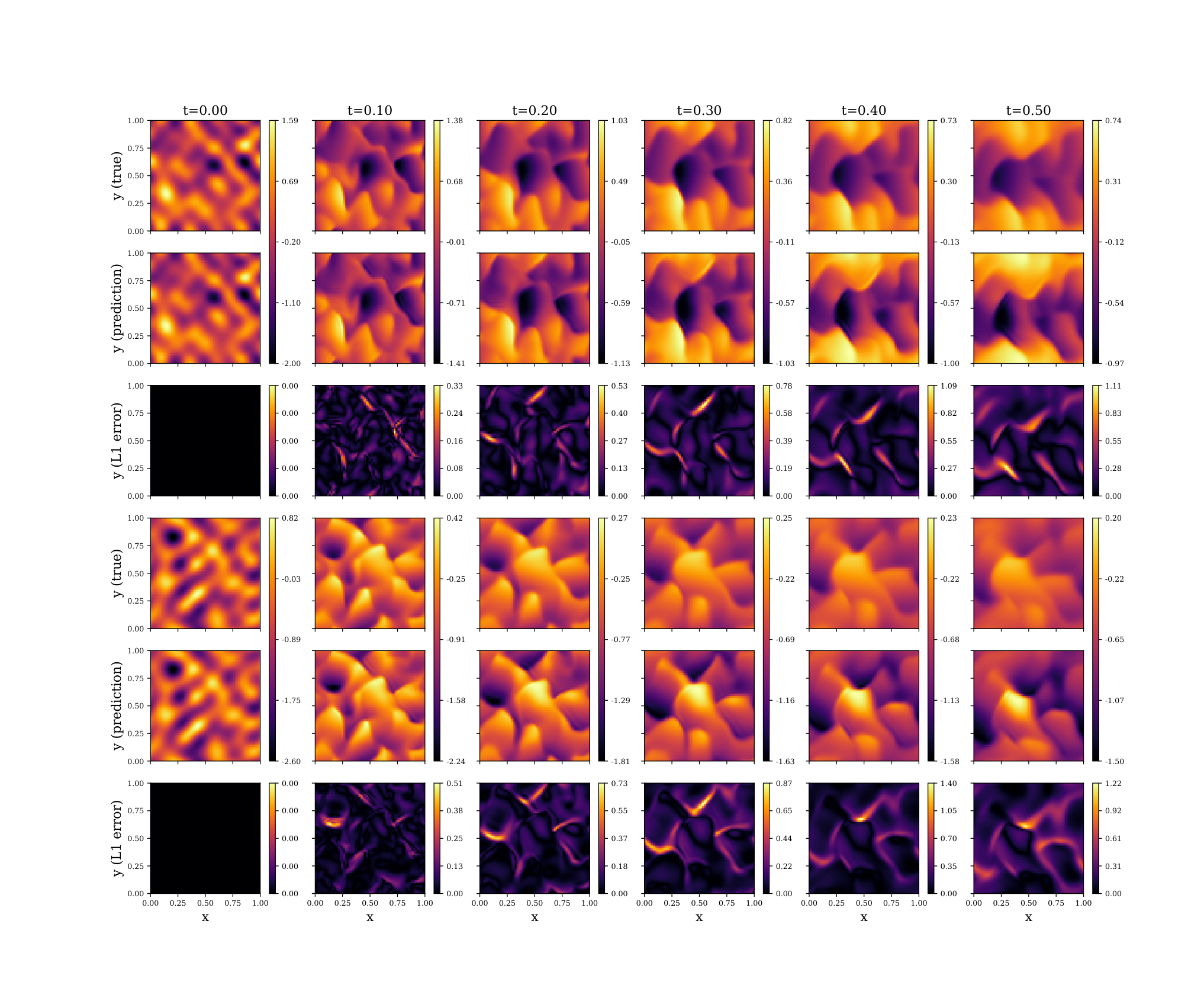
We trained the proposed GrADE using 120 samples of the initial condition and snapshots at three time instants only (i.e., last integration time index is 3). We allowed the learning rate to vary with number of epochs and trained the model for 501 epochs. For testing, we generated 20 additional realizations of the random initial conditions. Fig. 7 shows the the results corresponding to two initial conditions from the test dataset obtained using FeNICS and the proposed GrADE. The first and second rows depict the velocities (slices along $x$ and $y$ axes) obtained using FeNICS and the proposed approach respectively. Reasonable match among the results is observed. The third column shows the L1 error. Fig. 8 shows the velocities at different time-steps obtained using FeNICS and the proposed approach. Note that predicting the velocities for the 2D case as well is extremely difficult because of the formation of shocks. The fact that the proposed GrADE trained with observations at only three snapshots (with $\Delta t=0.02$) is able to provide reasonably accurate results is really impressive.

To understand the influence of last integration time index used during training, we perform case study by varying the last integration time index. The hyperparameter setting for all the cases are shown in Table 2. The results obtained are shown in Fig. 9. Unlike the 1D Burgers’ equation where the error was almost similar for all the cases, error is least when trained with last integration time index of 3. This is probably because the loss-function becomes extremely complex on increasing the last integration time index during training beyond 3. One way to address this issue is to use depth refinement. The idea is to alter depth of network during training. We use a smaller last integration time index during the initial training; however, as the training progresses, we start increasing the depth of the model. We recall that depth in GrADE refers to the number of time integration steps. This method enable us to train networks with more depth. The results corresponding to depth refinement are shown in Fig. 11. We start with a depth of 2 and gradually increased it till depth 4. Note that extra care is necessary with the depth refinement framework. The hyperparameters used are shown in Table 3. Results are compared with those obtained using a constant depth of 4. We observe that the computational time needed is less and the accuracy of the model is better for the depth refinement framework.

Next we concentrate on the role of attention model within the proposed framework. In this work, we have used FNN for computing the attention weights $\bm{\beta}$ and $\bm{\gamma}$. An alternative to this is to use Taylor net. SpiderConv proposed in [54] uses Taylor net in GNN for classification and segmentation tasks. It can be formulated as

where $p_{k}$ is element of $p\in\pi_{m}(\mathbb{R}^{2})$, $m$ is degree of polynomials, $Q$ is number of monomials and $w_{k}$ are trainable weights of networks. In Fig. 11, we present a comparative assessment between model accuracy when using FNN and Taylor net. We use $m=3,Q=10$ in Eq. (40). We observe that the results obtained using the FNN is slightly more accurate as compared to Taylor net. Recall that the output of the first graph network layer is supposed to yield the first derivative and those of the second layer is supposed to yield the second derivative. To validate the same, we plot the output of the two graph network layers in Fig. 12. Results obtained using central difference are also shown. A reasonably good match between the output of the graph network layers and those obtained using central difference is observed. This illustrates that the graph is able to capture the spatial derivatives.

References

- Zienkiewicz et al. [1977] Olgierd Cecil Zienkiewicz, Robert Leroy Taylor, Perumal Nithiarasu, and JZ Zhu. The finite element method, volume 3. McGraw-hill London, 1977.
- Moukalled et al. [2016] Fadl Moukalled, L Mangani, Marwan Darwish, et al. The finite volume method in computational fluid dynamics, volume 113. Springer, 2016.
- Liszka and Orkisz [1980] Tadeusz Liszka and Janusz Orkisz. The finite difference method at arbitrary irregular grids and its application in applied mechanics. Computers & Structures, 11(1-2):83–95, 1980.
- Aliabadi [2002] Mohammad H Aliabadi. The boundary element method, volume 2: applications in solids and structures, volume 2. John Wiley & Sons, 2002.
- Chakraborty and Zabaras [2018] Souvik Chakraborty and Nicholas Zabaras. Efficient data-driven reduced-order models for high-dimensional multiscale dynamical systems. Computer Physics Communications, 230:70–88, 2018. ISSN 0010-4655. doi: https://doi.org/10.1016/j.cpc.2018.04.007.
- Gao et al. [2020] Han Gao, Jian-Xun Wang, and Matthew J. Zahr. Non-intrusive model reduction of large-scale, nonlinear dynamical systems using deep learning. Physica D: Nonlinear Phenomena, 412:132614, 2020. ISSN 0167-2789. doi: https://doi.org/10.1016/j.physd.2020.132614.
- Xiu and Karniadakis [2002] Dongbin Xiu and George Em Karniadakis. The wiener–askey polynomial chaos for stochastic differential equations. SIAM Journal on Scientific Computing, 24(2):619–644, 2002. doi: 10.1137/S1064827501387826.
- Bilionis et al. [2013] Ilias Bilionis, Nicholas Zabaras, Bledar A. Konomi, and Guang Lin. Multi-output separable gaussian process: Towards an efficient, fully bayesian paradigm for uncertainty quantification. Journal of Computational Physics, 241:212–239, 2013. ISSN 0021-9991. doi: https://doi.org/10.1016/j.jcp.2013.01.011.
- Atkinson and Zabaras [2019] Steven Atkinson and Nicholas Zabaras. Structured bayesian gaussian process latent variable model: Applications to data-driven dimensionality reduction and high-dimensional inversion. Journal of Computational Physics, 383:166–195, 2019. ISSN 0021-9991. doi: https://doi.org/10.1016/j.jcp.2018.12.037.
- Schmidt and Lipson [2009] Michael Schmidt and Hod Lipson. Distilling free-form natural laws from experimental data. Science, 324(5923):81–85, 2009. ISSN 0036-8075. doi: 10.1126/science.1165893.
- Bongard and Lipson [2007] Josh Bongard and Hod Lipson. Automated reverse engineering of nonlinear dynamical systems. Proceedings of the National Academy of Sciences, 104(24):9943–9948, 2007. ISSN 0027-8424. doi: 10.1073/pnas.0609476104.
- Brunton et al. [2016] Steven L. Brunton, Joshua L. Proctor, and J. Nathan Kutz. Discovering governing equations from data by sparse identification of nonlinear dynamical systems. Proceedings of the National Academy of Sciences, 113(15):3932–3937, 2016. ISSN 0027-8424. doi: 10.1073/pnas.1517384113.
- Raissi and Karniadakis [2018] Maziar Raissi and George Em Karniadakis. Hidden physics models: Machine learning of nonlinear partial differential equations. Journal of Computational Physics, 357:125–141, 2018. ISSN 0021-9991. doi: https://doi.org/10.1016/j.jcp.2017.11.039.
- Patel and Desjardins [2018] Ravi G. Patel and Olivier Desjardins. Nonlinear integro-differential operator regression with neural networks, 2018.
- Geneva and Zabaras [2021] Nicholas Geneva and Nicholas Zabaras. Transformers for modeling physical systems, 2021.
- Nicholas Geneva [2020] Nicholas Zabaras Nicholas Geneva. Multi-fidelity generative deep learning turbulent flows. Foundations of Data Science, 2(4):391–428, 2020.
- Maulik et al. [2020] Romit Maulik, Romain Egele, Bethany Lusch, and Prasanna Balaprakash. Recurrent neural network architecture search for geophysical emulation. In Proceedings of the International Conference for High Performance Computing, Networking, Storage and Analysis, SC ’20. IEEE Press, 2020. ISBN 9781728199986.
- Geneva and Zabaras [2020] Nicholas Geneva and Nicholas Zabaras. Modeling the dynamics of pde systems with physics-constrained deep auto-regressive networks. Journal of Computational Physics, 403:109056, 2020. ISSN 0021-9991. doi: https://doi.org/10.1016/j.jcp.2019.109056.
- Wu and Xiu [2019] Kailiang Wu and Dongbin Xiu. Numerical aspects for approximating governing equations using data. Journal of Computational Physics, 384:200–221, 2019. ISSN 0021-9991. doi: https://doi.org/10.1016/j.jcp.2019.01.030.
- Lagaris et al. [1998] I.E. Lagaris, A. Likas, and D.I. Fotiadis. Artificial neural networks for solving ordinary and partial differential equations. IEEE Transactions on Neural Networks, 9(5):987–1000, 1998. doi: 10.1109/72.712178.
- Raissi et al. [2019] M. Raissi, P. Perdikaris, and G.E. Karniadakis. Physics-informed neural networks: A deep learning framework for solving forward and inverse problems involving nonlinear partial differential equations. Journal of Computational Physics, 378:686–707, 2019. ISSN 0021-9991. doi: https://doi.org/10.1016/j.jcp.2018.10.045.
- Wessels et al. [2020] Henning Wessels, Christian Weißenfels, and Peter Wriggers. The neural particle method–an updated lagrangian physics informed neural network for computational fluid dynamics. Computer Methods in Applied Mechanics and Engineering, 368:113127, 2020.
- Cai et al. [2021] Shengze Cai, Zhicheng Wang, Sifan Wang, Paris Perdikaris, and George Em Karniadakis. Physics-informed neural networks for heat transfer problems. Journal of Heat Transfer, 143(6):060801, 2021.
- Goswami et al. [2020] Somdatta Goswami, Cosmin Anitescu, Souvik Chakraborty, and Timon Rabczuk. Transfer learning enhanced physics informed neural network for phase-field modeling of fracture. Theoretical and Applied Fracture Mechanics, 106:102447, 2020.
- Chakraborty [2020] Souvik Chakraborty. Simulation free reliability analysis: A physics-informed deep learning based approach. arXiv preprint arXiv:2005.01302, 2020.
- Liu et al. [2020] Minliang Liu, Liang Liang, and Wei Sun. A generic physics-informed neural network-based constitutive model for soft biological tissues. Computer methods in applied mechanics and engineering, 372:113402, 2020.
- Zhu et al. [2019] Yinhao Zhu, Nicholas Zabaras, Phaedon-Stelios Koutsourelakis, and Paris Perdikaris. Physics-constrained deep learning for high-dimensional surrogate modeling and uncertainty quantification without labeled data. Journal of Computational Physics, 394:56–81, 2019.
- Chakraborty [2021] Souvik Chakraborty. Transfer learning based multi-fidelity physics informed deep neural network. Journal of Computational Physics, 426:109942, 2021.
- Meng and Karniadakis [2020] Xuhui Meng and George Em Karniadakis. A composite neural network that learns from multi-fidelity data: Application to function approximation and inverse pde problems. Journal of Computational Physics, 401:109020, 2020.
- Targ et al. [2016] Sasha Targ, Diogo Almeida, and Kevin Lyman. Resnet in resnet: Generalizing residual architectures. arXiv preprint arXiv:1603.08029, 2016.
- Chen et al. [2018a] Ricky TQ Chen, Yulia Rubanova, Jesse Bettencourt, and David Duvenaud. Neural ordinary differential equations. arXiv preprint arXiv:1806.07366, 2018a.
- Dupont et al. [2019] Emilien Dupont, Arnaud Doucet, and Yee Whye Teh. Augmented neural odes. In H. Wallach, H. Larochelle, A. Beygelzimer, F. d'Alché-Buc, E. Fox, and R. Garnett, editors, Advances in Neural Information Processing Systems, volume 32. Curran Associates, Inc., 2019.
- Zhuang et al. [2020] Juntang Zhuang, Nicha Dvornek, Xiaoxiao Li, Sekhar Tatikonda, Xenophon Papademetris, and James Duncan. Adaptive checkpoint adjoint method for gradient estimation in neural ode, 2020.
- Wang et al. [2009] Qiqi Wang, Parviz Moin, and Gianluca Iaccarino. Minimal repetition dynamic checkpointing algorithm for unsteady adjoint calculation. SIAM Journal on Scientific Computing, 31(4):2549–2567, 2009. doi: 10.1137/080727890.
- Veličković et al. [2018] Petar Veličković, Guillem Cucurull, Arantxa Casanova, Adriana Romero, Pietro Liò, and Yoshua Bengio. Graph attention networks, 2018.
- Qin et al. [2019] Tong Qin, Kailiang Wu, and Dongbin Xiu. Data driven governing equations approximation using deep neural networks. Journal of Computational Physics, 395:620–635, 2019.
- Pinkus [1999] Allan Pinkus. Approximation theory of the mlp model in neural networks. Acta Numerica, 8:143–195, 1999. doi: 10.1017/S0962492900002919.
- Bahdanau et al. [2014] Dzmitry Bahdanau, Kyunghyun Cho, and Yoshua Bengio. Neural machine translation by jointly learning to align and translate. arXiv preprint arXiv:1409.0473, 2014.
- Luong et al. [2015] Minh-Thang Luong, Hieu Pham, and Christopher D Manning. Effective approaches to attention-based neural machine translation. arXiv preprint arXiv:1508.04025, 2015.
- Zheng et al. [2017] Heliang Zheng, Jianlong Fu, Tao Mei, and Jiebo Luo. Learning multi-attention convolutional neural network for fine-grained image recognition. In Proceedings of the IEEE international conference on computer vision, pages 5209–5217, 2017.
- Rodriguez-Torrado et al. [2021] Ruben Rodriguez-Torrado, Pablo Ruiz, Luis Cueto-Felgueroso, Michael Cerny Green, Tyler Friesen, Sebastien Matringe, and Julian Togelius. Physics-informed attention-based neural network for solving non-linear partial differential equations. arXiv preprint arXiv:2105.07898, 2021.
- Vaswani et al. [2017] Ashish Vaswani, Noam Shazeer, Niki Parmar, Jakob Uszkoreit, Llion Jones, Aidan N Gomez, Łukasz Kaiser, and Illia Polosukhin. Attention is all you need. In Advances in neural information processing systems, pages 5998–6008, 2017.
- Murphy [2022] Kevin P. Murphy. Probabilistic Machine Learning: An introduction. MIT Press, 2022.
- Henaff et al. [2015] Mikael Henaff, Joan Bruna, and Yann LeCun. Deep convolutional networks on graph-structured data, 2015.
- Defferrard et al. [2016] Michaël Defferrard, Xavier Bresson, and Pierre Vandergheynst. Convolutional neural networks on graphs with fast localized spectral filtering. In D. Lee, M. Sugiyama, U. Luxburg, I. Guyon, and R. Garnett, editors, Advances in Neural Information Processing Systems, volume 29. Curran Associates, Inc., 2016.
- Levie et al. [2019] Ron Levie, Federico Monti, Xavier Bresson, and Michael M. Bronstein. Cayleynets: Graph convolutional neural networks with complex rational spectral filters. IEEE Transactions on Signal Processing, 67(1):97–109, 2019. doi: 10.1109/TSP.2018.2879624.
- Scarselli et al. [2009] Franco Scarselli, Marco Gori, Ah Chung Tsoi, Markus Hagenbuchner, and Gabriele Monfardini. The graph neural network model. IEEE Transactions on Neural Networks, 20(1):61–80, 2009. doi: 10.1109/TNN.2008.2005605.
- Hamilton et al. [2017] Will Hamilton, Zhitao Ying, and Jure Leskovec. Inductive representation learning on large graphs. In I. Guyon, U. V. Luxburg, S. Bengio, H. Wallach, R. Fergus, S. Vishwanathan, and R. Garnett, editors, Advances in Neural Information Processing Systems, volume 30. Curran Associates, Inc., 2017.
- Monti et al. [2017] F. Monti, D. Boscaini, J. Masci, E. Rodola, J. Svoboda, and M. M. Bronstein. Geometric deep learning on graphs and manifolds using mixture model cnns. In 2017 IEEE Conference on Computer Vision and Pattern Recognition (CVPR), pages 5425–5434, Los Alamitos, CA, USA, jul 2017. IEEE Computer Society. doi: 10.1109/CVPR.2017.576.
- Queiruga et al. [2020] Alejandro F Queiruga, N Benjamin Erichson, Dane Taylor, and Michael W Mahoney. Continuous-in-depth neural networks. arXiv preprint arXiv:2008.02389, 2020.
- Peterson [2009] Leif E Peterson. K-nearest neighbor. Scholarpedia, 4(2):1883, 2009.
- Chen et al. [2018b] Ricky T. Q. Chen, Yulia Rubanova, Jesse Bettencourt, and David Duvenaud. Neural ordinary differential equations. In Proceedings of the 32nd International Conference on Neural Information Processing Systems, NIPS’18, page 6572–6583, Red Hook, NY, USA, 2018b. Curran Associates Inc.
- Alnæs et al. [2015] Martin Alnæs, Jan Blechta, Johan Hake, August Johansson, Benjamin Kehlet, Anders Logg, Chris Richardson, Johannes Ring, Marie E Rognes, and Garth N Wells. The fenics project version 1.5. Archive of Numerical Software, 3(100), 2015.
- Xu et al. [2018] Yifan Xu, Tianqi Fan, Mingye Xu, Long Zeng, and Yu Qiao. Spidercnn: Deep learning on point sets with parameterized convolutional filters. September 2018.