A generalized stacked reinforcement learning method for sampled systems

RL showed remarkable performance in puzzles and video games [1, 2, 3], while also having demonstrated certain success in industrial tasks [4, 5]. Still, plain RL settings face performance guarantee requirements in industry, traditionally being addressed via classical control, such as MPC [6, 7, 8, 9, 10]. There is some promising research on hybridization of MPC with RL and, generally, learning-based methods. Offline learning hybrids of RL and MPC have been proposed in an attempt to augment the learning based estimation peculiar to RL with explicit computations of MPC (see , e. g., [11, 12, 13, 14]). Certain challenging control engineering tasks have been handled using novel online RL-MPC approaches [15], [16]. An online RL-MPC hybrid is known to produce safe policies for general affine systems with a quadratic stage cost [17]. Another online RL-MPC approach has been studied for nonlinear systems with discounted stage cost [18]. It can be seen that, although RL and MPC start off with fundamentally different optimal control problems (finite horizon vs. infinite horizon [19]), there is plenty of options to blend them for the sake of gaining the advantages of both. In this work, we study so-called stacked RL first proposed in [20] in the Q-learning format for discrete-time systems. Stacked RL is an approach that combines model-based computation of trajectories peculiar to MPC with learnable critics peculiar to RL. Unlike conventional methods of RL such as Q-learning and policy iteration, stacked RL is an online-learning method and thus it is intended to work “out of the box” without any pretraining, much like in the case of MPC. We generalize this approach to sample-and-hold systems and suggest a further variant of it called stacked RL-QV, where the optimal cost-to-go (or value, depending on the problem statement) function approximation is used as a terminal cost. This work concentrates on studying the performance of the suggested agents in experiments with a mobile robot, while the question of incorporating safety and stability constraints was addressed in [21, 22, 23].

The rest of the paper is organized as follows. A theoretical background is addressed in Section II. The description of the new stacked RL-QV algorithm and its theoretical analysis are given in Section III. Section IV is concerned with a particular practical realization of the algorithm. Experimental results and comparison with the stacked Q-learning as per [20], in the sample-and-hold variant, are given Section V.

Notation. For any $z$, denote $\{z_{i|k}\}_{i=1}^{N}\triangleq\{z_{1|k},\dots,z_{N|k}\}\triangleq\{z_{k},\dots,z_{k+N-1}\}$, $N\in\mathbb{N}$, if a starting index $k\in\mathbb{N}$ is emphasized; otherwise, it is just $\{z_{i}\}^{N}=\{z_{1},\dots,z_{N}\}$. If $N$ in the above is omitted, the sequence is considered infinite. The notation $[N]$ will mean the set $\{1,2,\dots,N\}$.

We consider an environment as a general non-linear dynamical system

where $x\in\mathbb{R}^{n}$ is the state, $u\in\mathbb{R}^{m}$ is the control action $u$, and $f:\mathbb{R}^{n}\times\mathbb{R}^{m}\rightarrow\mathbb{R}^{n}$ is the system dynamics function. The goal is to solve the following infinite-horizon optimal control problem:

where $x_{0}$ is the initial state, $r$ is the running cost, $\rho:\mathbb{R}^{n}\rightarrow\mathbb{R}^{m}$ is a control policy that belongs to some class of admissible policies $\mathcal{U}$ (we assume that all policies in $\mathcal{U}$ imply the convergence of the above integral and there exists a minimizer). Note, that unlike [18] our setup allows for undiscounted stage costs. This problem is given in the cost minimization format, as it is common in control, while RL usually treats $r$ as a reward and aims at its maximization. The integral cost is also called cost-to-go (analogously, reward-to-go). The optimum of the cost-to-go satisfies the Bellman optimality principle:

where $x^{\rho}(t)$ is the trajectory under the policy $\rho$. The respective minimizer $\rho^{*}$, that corresponds to $J^{*}$, is a (globally) optimal policy. Let $\eta$ be an arbitrary policy on $[0,t]$ (head policy). Then, the Bellman optimality principle can be rewritten in terms of a Q-function with an $\eta$ head:

Notice that there is, in general, no limiting case of a Q-function in the time-continuous case , i. e., where the head policy boils down to a single action.

In this section, we discuss stacked RL in a sampled setting. Let $\delta$ be a sampling step size so that the policy is updated every $\delta$ units of time. Fix an index $k\in\mathbb{N}$ and let us count sampled policies $\rho_{i|k}$ on $\delta$-intervals via an index $i\in\mathbb{N}$ starting at $k$. Then, the Q-function at the $i-1$st step reads:

where $x((k+i-1)\delta)$ is the starting state inside the sampling interval and $Q^{\delta}$ is the Q-function there. Let us use the shorthand notation, for a $j\in\mathbb{N}$, $x_{j}:=x(j\delta)$. Notice that a sampled state trajectory satisfies, for $t\in[(k+i-1)\delta,(k+i)\delta]$,

In the stacked RL setting, we consider a finite horizon of the described $\delta$-intervals, starting from every step $k$. Let the horizon be some $N\in\mathbb{N}$. Then, let $i$ run over $[N-1]$. Let us consider a stack of Q-functions as follows:

The optimization problem of the stacked RL-QV is suggested in the following form, while adding a $J^{*}$-terminal cost (cf. stacked Q-learning [20]):

Thus, the minimization is over a finite stack of sampled policies $\{\rho_{i|k}\}^{N-1}_{i=1}$. The next theorem shows that the optimal policy resulting from the Stacked RL-QV yields the globally optimally policy , i. e., the minimizer of $J^{*}$.

The following theorem illustrates how for a sufficiently high sampling frquency the difference between the two metrics in (8) is negligible.

In the next section, we discuss a particular realization of the stacked RL-QV algorithm using a double-critic for a sample-and-hold system, which is the simplest form of sampled system, in which the sampled policies simplify just to constant actions.

The sample-and-hold setting can be described as follows:

where $\mathcal{D}$ is a suitable derivative operator, $u^{\delta}$ is a control signal sampled at $\delta$-steps, $\rho:\mathbb{R}^{n}\rightarrow\mathbb{R}^{m}$ is a policy to be applied sample-wise, and $\delta>0$ is the sampling time as before. For any $k\in\mathbb{N}$, the state $x^{u_{k}}(t)$ at $t\geq k\delta$ under $u_{k}$ satisfies

When predicting these sampled states in practice, one has to use an approximation, in general , e. g., a numerical integration scheme. The Euler scheme is the simplest one:

where $\hat{x}_{i|k}$ denotes the approximate state. Whereas tabular methods of RL can effectively compute the Q- and/or value function, they are not suitable for online application, which is usually tackled using temporal-difference (TD). An actor-critic structure with neural networks is then employed to approximate the optimal Q- and/or value (or cost-to-go) function using the TD. In this work, we consider a double-critic structure, that approximates both, as follows:

where $w,v$ are the weights of the $\hat{Q}$- and $\hat{J}$-critic, respectively, $\varphi_{Q},\varphi_{V}$ are the corresponding activation functions, $\concat$ is the operator of concatenating vectors. We consider here shallow networks only for the ease of notation – deep topologies can be used analogously.

The critic objective can be formulated via an array of TDs formed from an experience replay as follows:

and $w_{k},v_{k}$ are the vectors of the critic neural network weights to be optimized over, $w_{k-1},v_{k-1}$ are the vectors of the weights from the previous time step, $M$ is the size of the experience replay.

The actor objective can be expressed in the following form, according to the stacked RL-QV principle:

The overall actor-critic realization of the stacked RL-QV in a sample-and-hold setting is summarized in Algorithm 1.

The stacked RL-QV was tested in mobile robot parking problem and compared to the stacked Q-learning based on [20] (further called stacked RL-Q for consistency) and an MPC agent.

The experiment consisted of a total of 150 runs. The robot started from different positions on a grid over an experimental polygon with a side of 4 m, turned away from the center – the target (see Fig 2). The goal was to park the robot at the target while achieving a desired orientation.

The model of the three-wheel robot was assumed in the following form:

where $x$ is the $x$-coordinate in [m], $y$ is the $y$-coordinate in [m], $\alpha$ is the orientation angle in [rad], $v$ is the linear velocity in [m/s], $\omega$ is the angular velocity in [rad/s]. The action is $u=[v|\omega]$.

The stage cost was taken in the following quadratic form:

where $\chi$ is equal either $\chi_{Q}$ or $\chi_{J}$ – the Q- and cost-to-go function regressor, respectively – $\chi_{Q}:=[(x,y,\alpha)|u]$, $\chi_{J}:=(x,y,\alpha)$, $R$ is a diagonal positive-definite matrix.

All the experiments were performed on a Robotis TurtleBot3 using a Robot Operating System (ROS) and a Python framework for RL called rcognita (see Fig. 1 and the Github link github.com/pavel-osinenko/rcognita for more details). Experiments were carried out in the following setups:

1. 1.

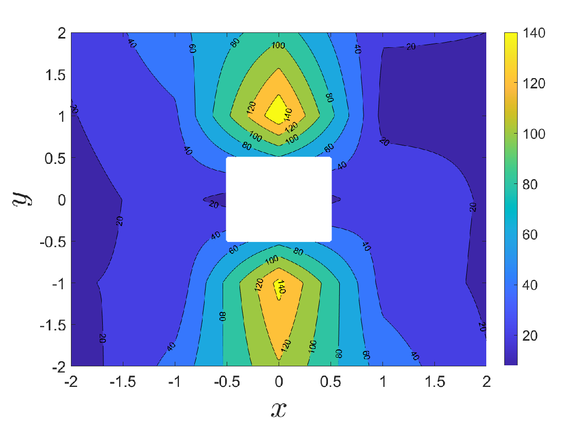
   Long-sighted horizon: $N=12,\delta=0.1s$. Here, the effective prediction horizon equals 1.2 seconds (see fig. 3);

2. 2.

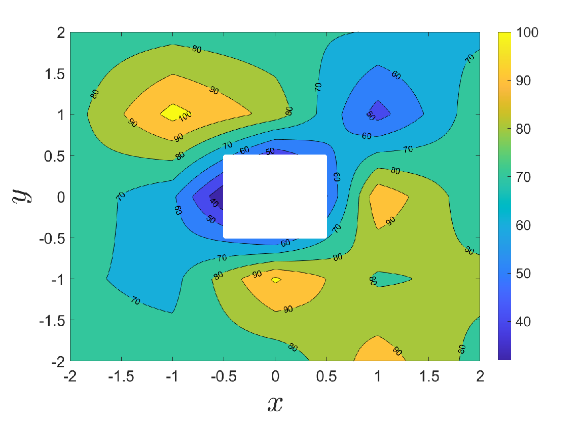
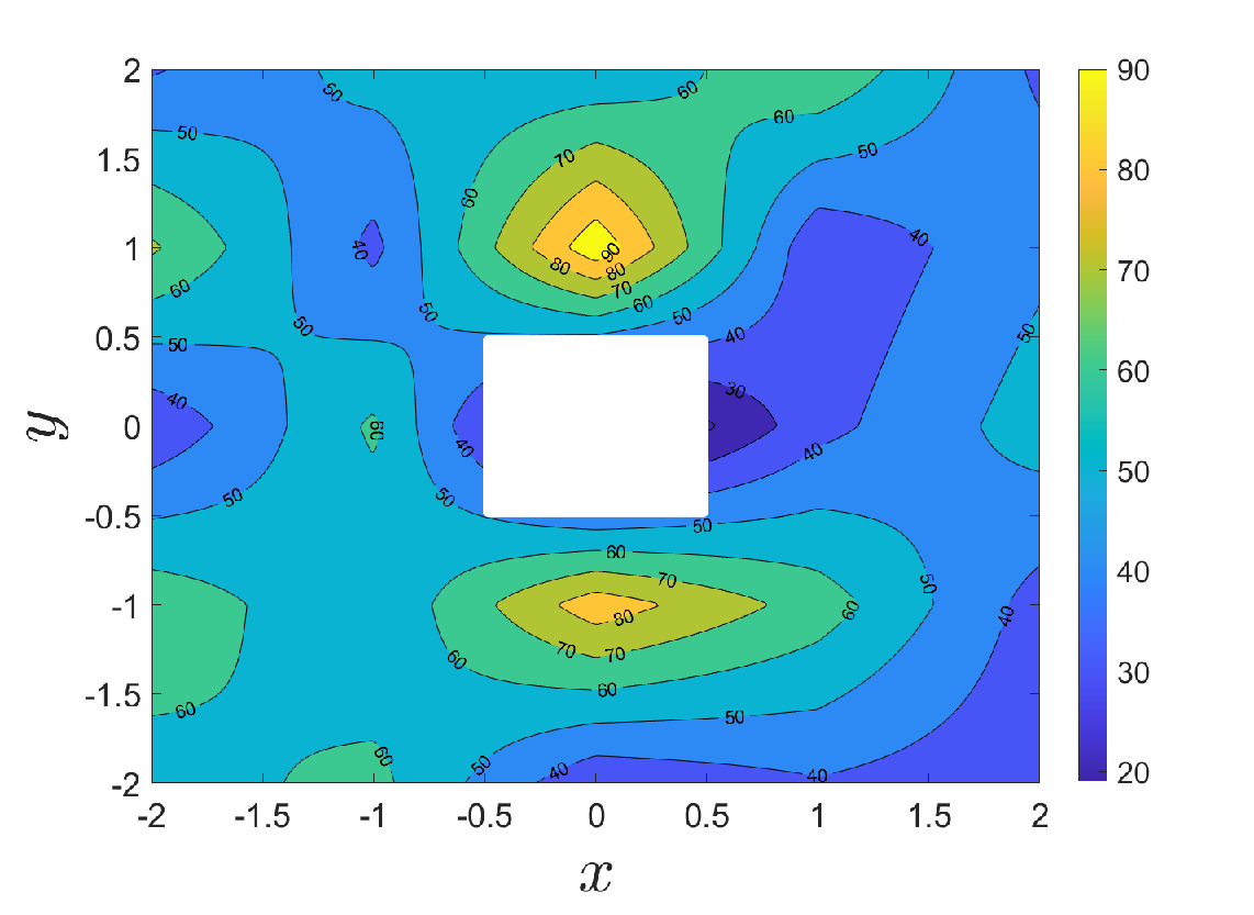
   Short-sighted horizon: $N=6,\delta=0.1s$. The effective prediction horizon equals 0.6 seconds (see fig. 4).

For each start on the grid, the accumulated stage costs $J_{\text{RL-Q}},J_{\text{RL-QV}},J_{\text{MPC}}$ were computed. The accumulated cost relationships

where then computed as performance marks.

The results of the cost difference percentage (20) are shown in Fig. 3a, 4a, while of (21) – in Fig. 3b, 4b.

It was observed that both the RL agents generally outperformed MPC in terms of the accumulated stage cost for both horizon setups (see Fig. 3–4). At the same time, the QV variant showed better results than the Q one. Notice that both have the same computational complexity for equal horizon. This indicated certain merits of the QV variant in the conducted experiment.

The results indicate that the advantage of the proposed stacked approaches over MPC strongly depends on the area of the state space, from which that agent begins its learning. It is also notable that both RL-Q and RL-QV seem to outperform MPC consistently for longer prediction horizons. Thus in a practical scenario, when MPC is done with the largest horizon that can be computed in a reasonable ammount of time, RL-Q and RL-QV seem to be superior to MPC.

References

• [1] D. Silver, T. Hubert, J. Schrittwieser, I. Antonoglou, M. Lai, A. Guez, M. Lanctot, L. Sifre, D. Kumaran, T. Graepel, T. Lillicrap, K. Simonyan, and D. Hassabis, “A general reinforcement learning algorithm that masters chess, shogi, and go through self-play,” Science, vol. 362, no. 6419, pp. 1140–1144, 2018.
• [2] C. Berner, G. Brockman, B. Chan, V. Cheung, P. Dkebiak, C. Dennison, D. Farhi, Q. Fischer, S. Hashme, C. Hesse, et al., “Dota 2 with large scale deep reinforcement learning,” arXiv preprint arXiv:1912.06680, 2019.
• [3] O. Vinyals et al., “Grandmaster level in StarCraft II using multi-agent reinforcement learning,” Nature, vol. 575, no. 7782, pp. 350–354, 2019.
• [4] J. Kober, J. A. Bagnell, and J. Peters, “Reinforcement learning in robotics: A survey,” The International Journal of Robotics Research, vol. 32, no. 11, pp. 1238–1274, 2013.
• [5] N. C. Luong, D. T. Hoang, S. Gong, D. Niyato, P. Wang, Y.-C. Liang, and D. I. Kim, “Applications of deep reinforcement learning in communications and networking: A survey,” IEEE Communications Surveys & Tutorials, vol. 21, no. 4, pp. 3133–3174, 2019.
• [6] N. Lazic, C. Boutilier, T. Lu, E. Wong, B. Roy, M. Ryu, and G. Imwalle, “Data center cooling using model-predictive control,” in Advances in Neural Information Processing Systems, S. Bengio, H. Wallach, H. Larochelle, K. Grauman, N. Cesa-Bianchi, and R. Garnett, Eds., vol. 31. Curran Associates, Inc., 2018, pp. 3814–3823. [Online]. Available: https://proceedings.neurips.cc/paper/2018/file/059fdcd96baeb75112f09fa1dcc740cc-Paper.pdf
• [7] D. Hrovat, S. Di Cairano, H. E. Tseng, and I. V. Kolmanovsky, “The development of model predictive control in automotive industry: A survey,” in 2012 IEEE International Conference on Control Applications, 2012, pp. 295–302.
• [8] M. G. Forbes, R. S. Patwardhan, H. Hamadah, and R. B. Gopaluni, “Model predictive control in industry: Challenges and opportunities,” IFAC-PapersOnLine, vol. 48, no. 8, pp. 531 – 538, 2015, 9th IFAC Symposium on Advanced Control of Chemical Processes ADCHEM 2015.
• [9] S. Kouro, M. A. Perez, J. Rodriguez, A. M. Llor, and H. A. Young, “Model predictive control: Mpc’s role in the evolution of power electronics,” IEEE Industrial Electronics Magazine, vol. 9, no. 4, pp. 8–21, 2015.
• [10] S. Vazquez, J. Rodriguez, M. Rivera, L. G. Franquelo, and M. Norambuena, “Model predictive control for power converters and drives: Advances and trends,” IEEE Transactions on Industrial Electronics, vol. 64, no. 2, pp. 935–947, 2016.
• [11] F. Berkenkamp, M. Turchetta, A. Schoellig, and A. Krause, “Safe model-based reinforcement learning with stability guarantees,” vol. 2017-December, 2017, pp. 909–919.
• [12] Y. Song and D. Scaramuzza, “Learning high-level policies for model predictive control.”
• [13] K. Napat, M. I. Valls, D. Hoeller, and M. Hutter, “Practical reinforcement learning for mpc: Learning from sparse objectives in under an hour on a real robot,” in 2nd Annual Conference on Learning for Dynamics and Control (L4DC 2020), 2020.
• [14] D. Hoeller, F. Farshidian, and M. Hutter, “Deep value model predictive control,” in Conference on Robot Learning, 2020, pp. 990–1004.
• [15] I. Lenz, R. A. Knepper, and A. Saxena, “Deepmpc: Learning deep latent features for model predictive control,” in Robotics: Science and Systems, 2015.
• [16] P. Drews, G. Williams, B. Goldfain, E. A. Theodorou, and J. M. Rehg, “Aggressive deep driving: Combining convolutional neural networks and model predictive control,” in Proceedings of the 1st Annual Conference on Robot Learning, ser. Proceedings of Machine Learning Research, S. Levine, V. Vanhoucke, and K. Goldberg, Eds., vol. 78. PMLR, 13–15 Nov 2017, pp. 133–142. [Online]. Available: http://proceedings.mlr.press/v78/drews17a.html
• [17] M. Zanon and S. Gros, “Safe reinforcement learning using robust mpc,” IEEE Transactions on Automatic Control, vol. 66, no. 8, pp. 3638–3652, 2021.
• [18] M. Bhardwaj, S. Choudhury, and B. Boots, “Blending mpc & value function approximation for efficient reinforcement learning,” arXiv preprint arXiv:2012.05909, 2020.
• [19] J. A. Primbs, V. Nevistić, and J. C. Doyle, “Nonlinear optimal control: A control lyapunov function and receding horizon perspective,” Asian Journal of Control, vol. 1, no. 1, pp. 14–24, 1999. [Online]. Available: https://onlinelibrary.wiley.com/doi/abs/10.1111/j.1934-6093.1999.tb00002.x
• [20] P. Osinenko, T. Göhrt, G. Devadze, and S. Streif, “Stacked adaptive dynamic programming with unknown system model,” IFAC-PapersOnLine, vol. 50, no. 1, pp. 4150–4155, 2017.
• [21] P. Osinenko, L. Beckenbach, T. Göhrt, and S. Streif, “A reinforcement learning method with closed-loop stability guarantee,” arXiv preprint arXiv:2006.14034, 2020.
• [22] L. Beckenbach, P. Osinenko, and S. Streif, “On closed-loop stability of model predictive controllers with learning costs,” in 2020 European Control Conference (ECC). IEEE, 2020, pp. 184–189.
• [23] L. Beckenbach, P. Osinenko, T. Göhrt, and S. Streif, “Constrained and stabilizing stacked adaptive dynamic programming and a comparison with model predictive control,” in 2018 European Control Conference (ECC). IEEE, 2018, pp. 1349–1354.
• [24] C. Tallec, L. Blier, and Y. Ollivier, “Making deep q-learning methods robust to time discretization,” in International Conference on Machine Learning, 2019.
• [25] K. Doya, “Reinforcement learning in continuous time and space,” vol. 12, no. 1, pp. 219–245, 2000.
• [26] H. Khalil, Nonlinear Systems. Prentice-Hall. 2nd edition, 1996.