A thesis presented to the Faculty of Science in partial fulfillment of the requirements for the degree of
Doctor Scientiarum (Dr. Scient.)
Towards Explainable Fact Checking
Preface
This document is a doktordisputats - a thesis within the Danish academic system required to obtain the degree of Doctor Scientiarum, in form and function equivalent to the French and German Habilitation and the Higher Doctorate of the Commonwealth.
This thesis documents and discusses my research in the field of content-based automatic fact checking, conducted in the period from 2016 to 2020. The first part of the thesis offers an executive summary, which provides a brief introduction to the field of fact checking for a broader computer science audience; a summary of this thesis’ contributions to science; a positioning of the contributions of this thesis in the broader research landscape of content-based automatic fact checking; and finally, perspectives for future work.
As this thesis is a cumulative one as opposed to a monograph, the remainder of this document contains in total 10 technical sections organised in 3 technical chapters, which are reformatted versions of previously published papers. While the chapters are all self-contained, they are arranged to follow the logical steps of a fact checking pipeline. Moreover, the methodology presented in Section 8 builds on Section 6, which in turn builds on Section 4. Thus, it is advised to read the chapters in the order they occur in.
Acknowledgements
This doktordisputats documents research within the area of Applied Computer Science, more specifically within Natural Language Processing. As such, to get from having an idea, including a detailed plan for the experimental setup, to results, which can be interpreted and written up in a paper, is a long and winding road, involving writing and debugging code, and starting and monitoring experiments on the computing cluster. I could therefore not have produced this thesis on my own, while also fulfilling my duties as a faculty member at the University of Copenhagen. I am therefore immensely grateful to all the early-career researchers for choosing to work with me and being inspired by my research vision.
In a similar vein, this research would not have been possible without external research funding. I should therefore like to give my sincere thanks to the funding programmes of the European Commission, which have funded most of the research in this thesis. The very first project I worked on related to fact checking was funded by the Commission, namely the PHEME FP7 project (grant No. 611233). Later on, two of my PhD students were supported by the Marie Skłodowska-Curie grant agreement No 801199. Moreover, two of my collaborators for research documented in this thesis were supported by EU grants, namely ERC Starting Grant Number 313695 and QUARTZ (721321, EU H2020 MSCA-ITN).
Next, I would like to thank my external collaborators and mentors over the years who supported and guided me. Working out how to succeed in academia is anything but easy, and would be even harder without positive role models and fruitful collaborations.
Last but not least, I would like to thank my partner, Barry, for his unwavering support, having read and provided useful comments on more of my academic writing than anyone else, including on this thesis.
Abstract
The past decade has seen a substantial rise in the amount of mis- and disinformation online, from targeted disinformation campaigns to influence politics, to the unintentional spreading of misinformation about public health. This development has spurred research in the area of automatic fact checking, from approaches to detect check-worthy claims and determining the stance of tweets towards claims, to methods to determine the veracity of claims given evidence documents.
These automatic methods are often content-based, using natural language processing methods, which in turn utilise deep neural networks to learn higher-order features from text in order to make predictions. As deep neural networks are black-box models, their inner workings cannot be easily explained. At the same time, it is desirable to explain how they arrive at certain decisions, especially if they are to be used for decision making. While this has been known for some time, the issues this raises have been exacerbated by models increasing in size, and by EU legislation requiring models to be used for decision making to provide explanations, and, very recently, by legislation requiring online platforms operating in the EU to provide transparent reporting on their services. Despite this, current solutions for explainability are still lacking in the area of fact checking.
A further general requirement of such deep learning based method is that they require large amounts of in-domain training data to produce reliable explanations. As automatic fact checking is a very recently introduced research area, there are few sufficiently large datasets. As such, research on how to learn from limited amounts of training data, such as how to adapt to unseen domains, is needed.
This thesis presents my research on automatic fact checking, including claim check-worthiness detection, stance detection and veracity prediction. Its contributions go beyond fact checking, with the thesis proposing more general machine learning solutions for natural language processing in the area of learning with limited labelled data. Finally, the thesis presents some first solutions for explainable fact checking.
Even so, the contributions presented here are only a start on the journey towards what is possible and needed. Future research should focus on more holistic explanations by combining instance- and model-based approaches, by developing large datasets for training models to generate explanations, and by collective intelligence and active learning approaches for using explainable fact checking models to support decision making.
Resume
I det forløbne årti har der været en betydelig stigning i mængden af mis- og desinformation online, fra målrettede desinformationskampagner til at påvirke politik til utilsigtet spredning af misinformation om folkesundhed. Denne udvikling har ansporet forskning inden for automatisk faktatjek, fra tilgange til at opdage kontrolværdige påstande og bestemmelse af tweets holdning til påstande til metoder til at bestemme rigtigheden af påstande, givet bevisdokumenter.
Disse automatiske metoder er ofte indholdsbaserede ved hjælp af naturlige sprogbehandlingsmetoder, som bruger dybe neurale netværk til at lære abstraktioner i data på højt niveau til klassificering. Da dybe neurale netværk er ‘black-box’-modeller, er der ikke direkte indsigt i, hvorfor modellerne når frem til deres forudsigelser. Samtidig er det ønskeligt at forklare, hvordan de når frem til bestemte forudsigelser, især hvis de skal benyttes til at træffe beslutninger. Selv om dette har været kendt i nogen tid, er problemerne, som dette rejser, blevet forværret af modeller, der stiger i størrelse, og af EU-lovgivning, der kræver, at modeller bruges til beslutningstagning for at give forklaringer, og for nylig af lovgivning, der kræver online platforme, der opererer i EU til at levere gennemsigtig rapportering om deres tjenester. På trods af dette mangler de nuværende løsninger til forklarlighed stadig inden for faktatjek.
Et yderligere generelt krav til en sådan ‘deep learning’ baseret metode er, at de kræver store mængder af i domæne træningsdata for at producere pålidelige forklaringer. Da automatisk faktatjek er et meget nyligt introduceret forskningsområde, er der få tilstrækkeligt store datasæt. Derfor er der behov for forskning i, hvordan man lærer af begrænsede mængder træningsdata, såsom hvordan man tilpasser sig til usete domæner.
Denne doktordisputats præsenterer min forskning om automatisk faktatjek, herunder opdagelse af påstande, og om de bør tjekkes (‘claim check-worthiness detection’), opdagelse af holdninger (‘stance detection’) og forudsigelse af sandhed (‘veracity prediction’). Dens bidrag går ud over faktatjek, idet afhandlingen foreslår mere generelle maskinindlæringsløsninger til naturlig sprogbehandling inden for læring med begrænsede mærkede data. Endelig præsenterer denne doktordisputats nogle første løsninger til forklarlig faktatjek.
Alligevel er bidragene, der præsenteres her, kun en start på rejsen mod hvad der er muligt og nødvendigt. Fremtidig forskning bør fokusere på mere holistiske forklaringer ved at kombinere instans- og modelbaserede tilgange, ved at udvikle store datasæt til træningsmodeller til generering af forklaringer og ved kollektiv intelligens og aktive læringsmetoder til brug af forklarlige faktatjekmodeller til støtte for beslutningstagning.
Publications
The following published papers are included in the text of this dissertation, listed in the order of their appearance:
- 1.
- 2.
- 3.
Augenstein et al. 2016
An earlier version of this work appeared as:- •
- 4.
Zubiaga et al. 2018
An earlier version of this work appeared as:- •
- 5.
- 6.
- 7.
- 8.
- 9.
- 10.
The papers listed below were published concurrently with my research on content-based automatic fact checking, and are unrelated or marginally related to the topic of this dissertation. Therefore, they are not included in it. They are listed here to indicate the broadness of my research and to contextualise the research presented in this dissertation. In chronological order, those papers are:
- 1.
- 2.
- 3.
- 4.
- 5.
- 6.
- 7.
- 8.
- 9.
- 10.
- 11.
- 12.
- 13.
- 14.
- 15.
- 16.
- 17.
- 18.
- 19.
- 20.
- 21.
- 22.
- 23.
- 24.
- 25.
- 26.
- 27.
- 28.
- 29.
- 30.
- 31.
- 32.
- 33.
- 34.
- 35.
- 36.
- 37.
- 38.
- 39.
- 40.
Finally, the following are, at the time of writing, unpublished manuscripts available on pre-print servers, which have been written concurrently with the research papers included in this dissertation. Some of them are strongly related to the topic of this dissertation, whereas others are not. As they are not yet accepted for publication, they do not fulfill the formal critera for inclusion into a doktordisputats at the Faculty of Science, University of Copenhagen. They are listed here to demonstrate my continued research efforts in the area of content-based automatic fact checking and related fields.
Part I Executive Summary
1
Executive Summary
1 Introduction
False information online is one of the greatest problems of the past decade, both from a societal and an individual decision making perspective. Among others, deliberate spreading of false information (disinformation) is being used to influence elections across the world (Bovet & Makse 2019; Juhász & Szicherle 2017; Howard & Kollany 2016; Derczynski et al. 2019; Ncube 2019), and accidental spreading of false information (misinformation) about public health in the wake of COVID-19 has led to what has been coined an ‘infodemic’ (Cuan-Baltazar et al. 2020; Kouzy et al. 2020; Brennen et al. 2020).
While manual journalistic efforts to curb false information are crucial (Waisbord 2018), they cannot scale to fact-checking hundreds of millions of daily Twitter posts. Consequently, detecting false information has become an important task to automate.
What follows hereafter is an introduction to the topic of automatic fact checking, covering fact checking sub-tasks, machine learning methods, as well as explainability methods. Where appropriate, this section cross-references the papers contained in the later methodological chapters. A more detailed introduction to the contributions of each paper can be subsequently found in Section 2.
1.1 Automatic Fact Checking
One typically differentiates automatic fact checking approaches by whether they are based on network or content information; we consider each of these in turn below.
1.1.1 Network-Based Approaches
Network-based approaches aim to identify false information purely based on interactions between people on e.g. social media platforms. Each social media user is connected to others in different ways, e.g. through following their posts, being followed or quoting users in posts. All these interactions together then form networks. Research has found that users in the same such networks often share common beliefs and, crucially here, that users spreading disinformation often tend to part of the same such networks.
To illustrate this, please find an example from a paper of mine (Hartmann et al. 2019) in Figure 1. The use case here is the visualisation of tweets around the crash of Malaysian Airlines (MH17) flight on 17 July 2014, on its way from Amsterdam to Kuala Lumpur over Ukrainian territory, resulting in the death of 298 civilians. The crash resulted in competing narratives around who was to blame – whether the plane was shot down by the Ukrainian military, or by Russian separatists in Ukraine supported by the Russian government (Oates 2016). The latter theory is the one subsequently confirmed by an international investigations team. The figure shows a retweet network, a graph that contains users as nodes and an edge between two users if at least one of the users retweets the other in a tweet that is detected to be on topic. Each edge is semi-automatically labelled as either pro-Russian, pro-Ukrainian or neutral, depending on the prevailing polarity of the content of the tweet being retweeted between users. As can be seen, the two networks corresponding to the two competing narratives are largely disconnected, i.e. they are being put forward by different groups of people. Based on such an analysis, disinformation can easily be detected, e.g. by flagging users11 1 At this point, it might be worth mentioning that not all such users are real people – many of them are bots. Bot detection, though, is beyond the scope of this thesis. who are part of disinformation networks.

1.1.2 Content-Based Approaches

A content-based automatic fact checking pipeline can be decomposed into the following tasks:
- 1.
Detection of check-worthy claims;
- 2.
Evidence retrieval and ranking;
- 3.
Stance detection;
- 4.
Veracity prediction.
1.1.3 Detection of check-worthy claims
An example of how this works for a given input is shown in Figure 2. Assume the statement ‘Immigrants are a drain on the economy’ is given. The first step would then be to determine if this statement constitutes a claim or an opinion and, if it constitutes a claim, whether or not that claim is worth fact checking (claim check-worthiness detection). Whether or not a claim is determined to be worth fact-checking is influenced by claim importance, which is subjective. Typically, only sentences unlikely to be believed without verification are marked as check-worthy. Furthermore, domain interests skew what is deemed check-worthy, which might e.g. only be certain political claims, or only celebrity gossip, depending on the application at hand. Lastly, claims can be very different in nature (Francis 2016). The main categories of claims are: 1) numerical claims involving numerical properties about entities and comparisons among them; 2) entity and event properties such as professional qualifications and event participants; 3) position statements such as whether a political entity supported a certain policy; 4) quote verification assessing whether the claim states precisely the source of a quote, its content, and the event at which it supposedly occurred. All of this already makes the first step in the fact checking pipeline, the detection of check-worthy claims, a surprisingly non-trivial task. A more in-depth discussion of these challenges can be found in Paper 1 (Section 2).
1.1.4 Evidence retrieval and ranking
Following this, if the statement indeed is a check-worthy claim, evidence documents which can be used to confirm or refute the claim are retrieved from the Web and ranked by their relevance to the claim (evidence retrieval and ranking). Note that the source of documents for retrieval can be restricted to certain domains, e.g. Wikipedia only, as done for the FEVER shared task and dataset (Thorne et al. 2018), the setup of which is used in Paper 9, contained in Section 10. Alternatively, the whole Web can be used as a source, in which case a search engine is often used in this part of the pipeline, as done for the MultiFC dataset presented in Paper 8, Section 9. Moreover, if the statement is a social media post, replies to this post can be used as evidence documents, as done in RumourEval Derczynski et al. 2017; Gorrell et al. 2019, the setting of which is used in Papers 4 (Section 5 and 6 (Section 7). For simplicity, some experimental settings skip this step altogether, assuming all relevant evidence is identified manually, as done in Paper 10 (Section 11). A less stark simplification, but a simplification nonetheless, is to assume all relevant evidence documents are provided, and merely have to be reranked, which is e.g. explored in Allein et al. 2020 (which has not been included in this thesis).
1.1.5 Stance detection
The next step is to determine if the evidence documents retrieved in the previous step agree with, disagree with or are neutral towards the claim. This step is typically referred to as either stance detection or textual entailment. More generally, the task can be called pairwise sequence classification, where a label corresponding to a pair of sequences is learned. The first sequence can be a claim, a headline, a premise, a hypothesis, or a target such as a person or a topic. There are many different labelling schemes for this task, ranging from simply ‘positive’ vs. ‘negative’ to a very fine-grained task with many different labels. This challenge is explored in more detail in Paper 5 (Section 6). Intuitively, this step is easier the more directly an evidence document discusses a claim – the less textual overlap there is between the two texts, the harder it to determine the stance automatically – which is discussed in Papers 3 (Section 4) and 8 (Section 9).
1.1.6 Veracity prediction
Lastly, given the predicted labels from the stance classifier for claim, evidence pairs obtained in Step 3, as well as a ranking of evidence pages obtained in Step 2, the overall veracity of the claim in question can be determined. As in stance detection, there exist many different labelling schemes for this step. In addition to fine-grained judgements about where on the scale from ‘completely true’ to ‘completely false’ a claim lies, labels such as ‘not enough information’ or ‘spins the truth’ are used. Solutions to this are discussed in great detail in Paper 8 (Section 9).
It should be noted at this point that what automatic fact checking models aim to predict is not the irrefutable, objective truth, but rather the veracity of a claim with respect to certain evidence documents. If there exists counter evidence, or important evidence is missing, but they are not available to the fact checking model in a machine-readable format, the model has no way of telling this. Thus, it is up to the person utilising the fact checking model to carefully examine how the model has arrived at its prediction. Supporting humans in this endeavour is possible through models which, as is the goal explored in this thesis, produce an explanation for the automatic fact-check. This is further described in Section 1.3.
An intuition behind some of the key machine learning challenges with building such automatic fact checking methods and how they are addressed in this thesis is given next.
1.2 Learning with Limited and Heterogeneous Labelled Data
A core methodological challenge addressed throughout this thesis is that most fact checking datasets are small in nature and apply different labelling schemes. Learning stable automatic fact checking models from those datasets thus presents a significant challenge.
This thesis proposes methods within the following areas to tackle this problem:
- 1.
Output space modelling;
- 2.
Multi-task learning;
- 3.
Transfer learning.
Automatic fact checking is, at its core, a classification task: each claim has to be categorised as belonging to one of a set of classes denoting the claim’s veracity. Hence, methods popular for text classification ought to be suitable for automatic fact checking as well. On a high level, standard text classification models take the input text (e.g. a claim, perhaps concatenated with an evidence sentence), transform it to higher-level abstract features using a feature transformation function, and output a class label.
1.2.1 Output space modelling
While this works well for most purposes, this formulation has several shortcomings, which can be addressed by different ways of modelling the output space. First of all, with classes simply being represented by IDs, the inherent meaning of these classes is not directly represented by the model. Moreover, in fact checking, different veracity labels represent fine-grained nuances in meaning, e.g. ‘partly true’, ‘mostly true’, ’more evidence needed’, i.e. there is a relationship between labels. Thus, this thesis proposes to not just learn input features, but also output features for fact checking, more concretely, label embeddings, which capture the semantic relationships between labels. Papers 5 (Section 6) and 8 (Section 9) show that this trick can be applied to not just improve the performance of pairwise sequence classification and veracity prediction models, respectively, but also to unify label schemes from different datasets, without having to attempt to do this unification manually.
Moreover, Paper 3 (Section 4) applies a similar idea to the task of unseen target stance detection – i.e. determining the stance towards a target (e.g. a person or topic) that is unseen at test time. Prior to that, ordinarily, approaches would consist of one model per stance target. By representing the targets as features as well and training a joint model, the resulting model can make stance predictions for any target, a formulation which resulted in state-of-the-art performance at the time.
Lastly, another form of output space modelling investigated in Paper 4 (Section 5) concerns the context of the target instance. As mentioned before, one task formulation of fact checking is detecting the veracity of rumours, where a rumour is verified by determining the stance of social media posts towards a rumour. As social media posts do not appear in isolation but, more often than not, are replies to previous posts, modelling them in isolation would mean losing out on important context. Therefore, this thesis proposes to frame rumour stance detection as a structured prediction task. The conversational structure on Twitter can be viewed as a tree, in turn consisting of branches that are made up of sequences of posts. We propose to treat each such branch as an instance. The labels for posts are then predicted in a sequential fashion, such that the model which makes these predictions has access to the posts as well as the predicted labels in the same conversational thread.
1.2.2 Multi-task learning
Different label schemes having been dealt with, another challenge concerns the generally low number of training instances of fact checking datasets – especially the earlier datasets such as Mohammad et al. 2016; Pomerleau & Rao 2017; Derczynski et al. 2017; Wang 2017 only contain around a couple of thousand training instances. Deep learning based text classification models tend to perform better the more examples they have available at training time. Moreover, with a paucity of training instances, they tend to struggle to even outperform simply predicting a random label or the most frequent label (see e.g. Hartmann et al. 2019). Two streams of research are explored in this thesis to tackle this problem – multi-task and transfer learning – both of which build on the general idea of obtaining more training data from other sources.
Multi-task learning is the idea of, in addition to the target task, obtaining training data for so-called auxiliary tasks. The latter are tasks which are often related to the target task, be it in form (i.e. if the target task is a text classification task, those would also be text classification tasks); in domain (e.g. the target task and auxiliary task data could all be from the legal domain); or in the nature of the task (e.g. only taking into consideration different variants of sentiment analysis). The idea is then to train a model on all such tasks at once, but to only utilise the predictions of the target task.
Deep neural network based text classification models typically consist of an: 1) input layer, which maps inputs to features, 2) hidden layers, which learn more abstract higher-order features; and 3) an output layer, which maps the features from the hidden layer to output labels. Since inputs as well as the type and number of classes tends to differ by task, in multi-task learning, only the hidden layers tend to be shared between tasks, whereas the input and output layers tend to be kept separate for each task. Intuitively, sharing the hidden layer means the model can better learn abstract features by having seen more examples. Training on several tasks at the same time also has a regularisation effect – it is more difficult for a model to overfit to spurious patterns for any one task if it is trained to perform several tasks at the same time. In this thesis, multi-task learning is used as a building block in several papers. In Papers 5 (Section 6) and 8 (Section 9), it is combined with the idea of label embeddings. In Papers 9 (Section 10) and 10 (Section 11), it is used as a way of specifically instilling different types of knowledge in a model – about semantic coherence and how to generate adversarial claims (Paper 9), and about veracity and how to generate instance-level explanations (Paper 10).
1.2.3 Transfer learning
Finally, this thesis examines transfer learning as a way of increasing the amount of training data for a task. Transfer learning can be seen as as special form of multi-task learning where a model is trained on several tasks, but instead of it being trained on several tasks at once, it is trained on several tasks sequentially. The last one of these tasks is typically the target task, unless there is no training data available for the target task at all, in which case one typically speaks of unsupervised or zero-shot transfer learning. The other tasks are typically referred to as the source tasks.
As with multi-task learning, the intuition that is typically applied is that the closer the source tasks are to the target task, be it in terms of form, domain, text type, or application task considered, the more likely it is to benefit the target task. The current de-facto approach to natural language processing at the time of writing is the so-called ‘pre-train, then fine-tune’ approach, where sentence encoding models are pre-trained on unsupervised tasks which require no manual annotation. The overall goal is for this pre-training procedure to result in a better initialisation of the hidden layers of a deep neural network, such that when it is fine-tuned for a target task, it converges more quickly and is less likely to get stuck in local minima. There are many different variants of such pre-training tasks for NLP, such as simple next-word prediction (language modelling), next-sentence prediction or term frequency prediction (Aroca-Ouellette & Rudzicz 2020). These pre-trained models, often pre-trained on large amounts of raw data, can then be re-used across different applications in a plug-and-play fashion, and a large number of such pre-trained models have been published in the last year alone Rogers et al. 2020.
This thesis is not concerned with learning better unsupervised representations from large amounts of data as such – though it does utilise such pre-trained models. Instead, it focuses on how to better fine-tune them for given target tasks. Three different types of fine-tuning settings are explored. Paper 1 (Section 2) explores the common setting where relatively little target-task data is available, but noisy training data for the same task, albeit from a different domain, is available. The paper then deals with how best to fine-tune a claim check-worthiness detection model in two steps – first on the out-of-domain data, then on the in-domain data. Paper 2 (Section 3) assumes no training data is available at all for the target domain. Instead, multiple training datasets for the same task, though from other domains, are available. Thus, the task becomes one of unsupervised multi-source domain adaptation. Lastly, Paper 6 (Section 7) addresses the problem that language, and thus test data, changes over time. To reflect that change, the paper proposes to perform sequential temporal domain adaptation, where models are adapted to more recent data sequentially, and shows that this improves performance.
1.3 Explainable Natural Language Understanding
The last vertical of relevance to fact checking is how to make fact checking models more transparent, such that end users can understand: 1) what a model as a whole has learned (model interpretabilty as well as 2) why a model produces a certain prediction for a certain instance (model explainability). Note here that the terms ‘interpretability’ and ‘explainability’ are often conflated in the literature, not least because an explainable model is often also interpretable.
The methods for explainable natural language understanding researched in this thesis can be divided into the following streams of approaches:
- 1.
Generating natural language explanations;
- 2.
Generating adversarial examples;
- 3.
Post-hoc explainability methods.
These are considered in turn below.
1.3.1 Generating natural language explanations
The inner workings of deep neural networks are, as already mentioned, relatively complex; especially since modern models have too many parameters to inspect them individually. One solution to this is to generate natural language explanations, based on the assumption that the easiest explanations to understand for users are those written in natural language.
The overall aim to produce free text (typically a sentence or a paragraph) that succinctly explains how the model has arrived at a certain prediction. Technically, this is achieved by training a model to both solve the main task and generate a textual explanation. In Paper 10 (Section 11), we approach this using multi-task learning. Ideally, such a free text explanation would be directly generated from a model’s hidden layers as an unsupervised task, however, this is extremely challenging to do. In Paper 10, we show that generating free-text explanations for fact checking is possible in a simplified setting. Namely, the model is given long articles written by journalists discussing evidence documents, and the model is trained to summarise those evidence documents, while also predicting the veracity of the corresponding claim. The summaries, in turn, represent justifications for the fact-check and thus an explanation for the respective fact checking label.
1.3.2 Generating adversarial examples
Another way of interpreting what a model has learned is to try to reveal systemic vulnerabilities of the model. Sometimes, usually because a model is trained on biased and/or small amounts of training data, it learns spurious correlations resulting in features that are red herrings – which a model has only seen a handful of times at training time, which were always associated with only one label, but which, in reality, are not indicative of the label. An example from the fact checking domain could be if a model is only exposed to false claims mentioning certain people, then it will very likely learn to always predict the veracity of ‘false’ whenever this name occurs in a claim.
The goal of generating adversarial examples is to identify such features, sometimes also called ‘universal adversarial triggers’, and use them to automatically generate instances which a fact checking model would predict an incorrect label for. This not only tells a user what a model would likely struggle with, but the automatically generated adversarial instances can in turn be used to improve models.
In Paper 10 (Section 10), we explore how to generate adversarial claims for fact checking. There are some additional challenges when researching this method for fact checking. First, the generated adversarial claims should contain these additional triggers, but without changing the meaning of the claim to the extent that they would change the ground truth label. To build on the example above, a trigger could be a certain name, which would not change the meaning of a claim, but could change what a fact checking model would predict for it. It could also be the word ‘not’, which in most cases would change the underlying meaning. The more different veracity labels are considered, the more difficult this becomes. Morever, generating a syntactically valid and semantically coherent claim is also non-trivial. While previous work generated claims from templates, this restricts the range of claim types that can be generated. We instead research how to do this automatically, using large language models, which generate these claims from scratch.
1.3.3 Post-hoc explainability methods
Lastly, another explainability technique explored in this thesis is post-hoc explainability. Unlike the approaches presented for generating natural language explanations and discovering universal adversarial triggers, post-hoc explainability methods are methods that can be applied after a model for a certain application task has already been trained. The general idea is to find regions of the input which best explain the predicted label for the corresponding instance. These regions of the input are typically called ‘rationales’, and are portions of the input text – words, phrases or sentences – which are salient for the predicted label given the trained model.
This can then very easily tell a user if a model focuses on the correct parts of the input or the incorrect parts of the input. Following up from the example above, in Section 1.3.2, an undesired part of the input to focus on for fact checking could be a person’s name in a claim, as this could be a reflection of the data selection process more than a reflection of the real world.
At the time of running experiments, and also of writing this thesis, there are no fact checking datasets annotated with human rationales. Veracity prediction models take not only claims as their input, but also evidence pages. As such, rationales would have to relate portions of claims and evidence pages, requiring a conceptually different annotation scheme than currently used. Therefore, Paper 8 (Section 8) focuses only on the subtask of fact checking which determines the relationship between two input texts, i.e. stance detection / natural language inference.
Paper 8 addresses the highly challenging task of automatically evaluating such post-hoc explainability methods. First off, they should of course be in line with human annotations, but these are not always available, and besides, should not be the only thing taken into account – for instance, an explanation should also be faithful to what the respective model has learned. The paper proposes different so-called ‘diagnostic properties’ for evaluating post-hoc explanations, and uses them to compare different types of post-hoc explainability methods across different classification tasks and datasets. Some of the findings are that different explainability methods produce very different explanations, and that explanations further differ by model. Different explanations can all be correct in their own way, e.g. they might offer true alternative explanations, which is just one of the things that makes explainability research challenging.
2 Scientific Contributions
Having given a general introduction to the topic of fact checking and the core challenges tackled in this thesis, this section now turns to describing the scientific contributions made by this thesis in more depth.
The core scientific contributions of models presented in thesis can be conceptualised along three axes:
Table 1 indicates where along these three axes each of the ten papers that make up this thesis are located. What follows next is a brief summary of the contributions of each paper, grouped by the ‘fact checking sub-task’ axis, following the structure of this thesis.22 2 The exception to this is evidence retrieval and reranking. As this is only a contribution in Paper 9, and there does not present the main contribution, this fact checking sub-task neither has its own subsection below, nor its own chapter in the thesis.
| FC Subtask | LLD Method | Explainability Method | ||||||||
| Claims | Evidence | Stance | Veracity | Output space | Multi-task | Transfer | Natural language | Adversarial | Post-hoc | |
| Augenstein et al. 2016 | X | X | ||||||||
| Zubiaga et al. 2018 | X | X | ||||||||
| Augenstein et al. 2018 | X | X | X | |||||||
| Augenstein et al. 2019 | X | X | X | X | ||||||
| Bjerva et al. 2020a | X | X | ||||||||
| Wright & Augenstein 2020 | X | X | ||||||||
| Wright & Augenstein 2020a | X | X | ||||||||
| Atanasova et al. 2020a | X | X | X | |||||||
| Atanasova et al. 2020 | X | X | ||||||||
| Atanasova et al. 2020b | X | X | X | X | ||||||
2.1 Detecting Check-Worthy Claims
The first fact checking area in which contributions are made concerns the detecting of check-worthy claims.
2.1.1 Paper 1: Positive Unlabelled Learning

This paper addresses the fact checking sub-task of claim check-worthiness detection, a text classification problem where, given a statement, one must predict if the content of that statement makes “an assertion about the world that is checkable” (Konstantinovskiy et al. 2018). There are multiple isolated lines of research which have studied variations of this problem: rumour detection on Twitter (Zubiaga et al. 2016b; Zubiaga et al. 2018), check-worthiness ranking in political debates and speeches (Nakov et al. 2018; Elsayed et al. 2019; Barrón-Cedeño et al. 2020), and ‘citation needed’ detection on Wikipedia (Redi et al. 2019) (see Figure 3). Each task is concerned with a shared underlying problem: detecting claims which warrant further verification. However, no work has been done to compare all three tasks to understand shared challenges in order to derive shared solutions, which could enable the improvement of claim check-worthiness detection systems across multiple domains. Therefore, we ask the following main research question in this work: are these (rumour detection on Twitter, check-worthiness ranking in political debates, ‘citation needed’ detection) all variants of the same task (claim check-worthiness detection), and if so, is it possible to have a unified approach to all of them?
In more detail, the contributions of this work are as follows:
- 1.
The first thorough comparison of multiple claim check-worthiness detection tasks.
- 2.
Positive Unlabelled Conversion (PUC), a novel extension of PU learning to support check-worthiness detection across domains.
- 3.
Results demonstrating that a unified approach to check-worthiness detection is achievable for 2 out of 3 tasks, improving over the state-of-the-art for those tasks.
2.1.2 Paper 2: Transformer Based Multi-Source Domain Adaptation

Multi-source domain adaptation is a well studied problem in deep learning for natural language processing. An example of this setting can be found in Figure 4: a model may e.g. be trained to predict the sentiment of product reviews for DVDs, electronics, and kitchen goods, and must utilise this learned knowledge to predict the sentiment of a review about a book. Proposed methods have been primarily studied using convolutional nets (CNNs) and recurrent nets (RNNs) trained from scratch, while the NLP community has recently begun to rely more and more on large pretrained transformer (LPX) models e.g. BERT (Devlin et al. 2019). To date there has been some preliminary investigation of how LPX models perform under domain shift in the single source-single target setting (Ma et al. 2019a; Han & Eisenstein 2019; Rietzler et al. 2020; Gururangan et al. 2020). What is lacking is a study into the effects of and best ways to apply classic multi-source domain adaptation techniques with LPX models, which can give insight into possible avenues for improved application of these models in settings where there is domain shift.
Given this, Paper 2 presents a study into unsupervised multi-source domain adaptation techniques for large pretrained transformer models, evaluating the proposed models on the tasks of rumour detection on Twitter as well as sentiment analysis of customer reviews. Our main research question is: do mixture of experts and domain adversarial training offer any benefit when using LPX models? The answer to this is not immediately obvious, as such models have been shown to generalize quite well across domains and tasks while still learning representations which are not domain invariant. Therefore, we experiment with four mixture of experts models, including one novel technique based on attending to different domain experts; as well as domain adversarial training with gradient reversal. Perhaps surprisingly, we find that, while domain adversarial training helps the model learn more domain invariant representations, this does not always result in increased target task performance. When using mixture-of-experts models, we see significant gains on out-of-domain rumour detection, and some gains on out-of-domain sentiment analysis. Further analysis reveals that the classifiers learned by domain expert models are highly homogeneous, making it challenging to learn a better mixing function than simple averaging.
2.2 Stance Detection
The second fact checking area in which contributions are made concerns the classification of stance and textual entailment.
2.2.1 Paper 3: Bidirectional Conditional Encoding
The goal of stance detection is to classify the attitude expressed in a text, towards a given target, here, as “positive”, ”negative”, or ”neutral”. The focus of this paper is on a novel stance detection task, namely tweet stance detection towards previously unseen target entities (mostly entities such as politicians or issues of public interest), as defined in the SemEval Stance Detection for Twitter task (Mohammad et al. 2016). This task is rather difficult, firstly due to not having training data for the targets in the test set, and secondly due to the targets not always being mentioned in the tweet. Thus the challenge is twofold. First, we need to learn a model that interprets the tweet stance towards a target that might not be mentioned in the tweet itself. Second, we need to learn such a model without labelled training data for the target with respect to which we are predicting the stance.
To address these challenges, we develop a neural network architecture based on conditional encoding (Rocktäschel et al. 2016), visualised in Figure 5. A long-short term memory (LSTM) network (Hochreiter & Schmidhuber 1997) is used to encode the target, followed by a second LSTM that encodes the tweet using the encoding of the target as its initial state. We show that this approach achieves better F1 than standard stance detection baselines, or an independent LSTM encoding of the tweet and the target. Results improve further with a bidirectional version of our model, which takes into account the context on either side of the word being encoded. In the shared task, this would be the second best result, except for an approach which uses automatically labelled tweets for the test targets. Lastly, when our bidirectional conditional encoding model is trained on such data, it achieves state-of-the-art performance.
2.2.2 Paper 4: Discourse-Aware Rumour Classification
[depth=0] u1: These are not timid colours; soldiers back guarding Tomb of Unknown Soldier after today’s shooting #StandforCanada –PICTURE– [support]
[depth=1] u2: @u1 Apparently a hoax. Best to take Tweet down. [deny]
[depth=1] u3: @u1 This photo was taken this morning, before the shooting. [deny]
[depth=1] u4: @u1 I don’t believe there are soldiers guarding this area right now. [deny]
[depth=2] u5: @u4 wondered as well. I’ve reached out to someone who would know just to confirm that. Hopefully get response soon. [comment]
[depth=3] u4: @u5 ok, thanks. [comment]
In this work we focus on the development of stance classification models for rumour detection. It has been argued that it could be helpful in determining the likely veracity to aggregate across multiple distinct stances in the multiple tweets discussing a rumour. This would provide, for example, the means to flag highly disputed rumours as being potentially false (Malon 2018). This approach has been justified by recent research that has suggested that the aggregation of the different stances expressed by users can be used for determining the veracity of a rumour (Derczynski et al. 2015a; Liu et al. 2015).
In this work, we examine in depth the use of so-called sequential approaches to the rumour stance classification task. Sequential classifiers are able to utilise the discursive nature of social media (Tolmie et al. 2017), learning from how ‘conversational threads’ evolve for a more accurate classification of the stance of each tweet – see Figure 6 for an example of such a conversational thread.
The work presented here advances research in rumour stance classification by performing an exhaustive analysis of different approaches to this task. In particular, we make the following contributions:
- •
We perform an analysis of whether – and the extent to which – the use of the sequential structure of conversational threads can improve stance classification in comparison to a classifier that determines a tweet’s stance from the tweet in isolation. To do so, we evaluate the effectiveness of a range of sequential classifiers: (1) a state-of-the-art classifier that uses Hawkes Processes to model the temporal sequence of tweets (Lukasik et al. 2016a); (2) two different variants of Conditional Random Fields (CRF), i.e., a linear-chain CRF and a tree CRF; and (3) a classifier based on Long Short Term Memory (LSTM) networks. We compare the performance of these sequential classifiers with non-sequential baselines, including the non-sequential equivalent of CRF, a Maximum Entropy classifier.
- •
We perform a detailed analysis of the results broken down by dataset and by depth of tweet in the thread, as well as an error analysis to further understand the performance of the different classifiers. We complete our analysis of results by delving into the features, and exploring whether and the extent to which they help characterise the different types of stances.
Our results show that sequential approaches do perform substantially better in terms of macro-averaged F1 score, proving that exploiting the dialogical structure improves classification performance. Specifically, the LSTM achieves the best performance in terms of macro-averaged F1 scores, with a performance that is largely consistent across different datasets and different types of stances. Our experiments show that LSTMs performs especially well when only local features are used, as compared to the rest of the classifiers, which need to exploit contextual features to achieve comparable – yet still inferior – performance scores. Our findings reinforce the importance of leveraging conversational context in stance classification. Our research also sheds light on open research questions that we suggest should be addressed in future work. Our work here complements other components of a rumour classification system that we implemented in the PHEME project, including a rumour detection component (Zubiaga et al. 2016a; Zubiaga et al. 2017), as well as a study into the diffusion of – and reactions to – rumour (Zubiaga et al. 2016b).
2.2.3 Paper 5: Multi-Task Learning Over Disparate Label Spaces

Contemporary work in multi-task learning for NLP typically focuses on learning representations that are useful across tasks, often through hard parameter sharing of hidden layers of neural networks (Collobert et al. 2011; Søgaard & Goldberg 2016). If tasks share optimal hypothesis classes at the level of these representations, multi-task learning leads to improvements (Baxter 2000). However, while sharing hidden layers of neural networks is an effective regulariser (Søgaard & Goldberg 2016), we potentially lose synergies between the classification functions trained to associate these representations with class labels. This paper sets out to build an architecture in which such synergies are exploited, with an application to pairwise sequence classification tasks (topic-based, target-depending and aspect-based sentiment analysis; stance detection; fake news detection; and natural language inference).
For many NLP tasks, disparate label sets are weakly correlated, e.g. part-of-speech tags correlate with dependencies (Hashimoto et al. 2017), sentiment correlates with emotion (Felbo et al. 2017; Eisner et al. 2016), etc. We thus propose to induce a joint label embedding space using a Label Embedding Layer that allows us to model these relationships, which we show helps with learning. A visualisation of the learned label embedding space is provided in Figure 7.
In addition, for tasks where labels are closely related, we should be able to not only model their relationship, but also to directly estimate the corresponding label of the target task based on auxiliary predictions. To this end, we propose to train a Label Transfer Network jointly with the model to produce pseudo-labels across tasks.
In summary, our contributions are as follows.
- 1.
We model the relationships between labels by inducing a joint label space for multi-task learning.
- 2.
We propose a Label Transfer Network that learns to transfer labels between tasks and propose to use semi-supervised learning to leverage them for training.
- 3.
We evaluate multi-task learning approaches on a variety of classification tasks and shed new light on settings where multi-task learning works.
- 4.
We perform an extensive ablation study of our model.
- 5.
We report state-of-the-art performance on topic-based sentiment analysis.
2.2.4 Paper 6: Temporal Domain Adaptation with Sequential Alignment
Evolution of language usage affects natural language processing tasks and, as such, models based on data from one point in time cannot be expected to generalise to the future. For example, the names ‘Bert’ and ‘Elmo’ would only rarely make an appearance prior to 2018 in the context of scientific writing. After the publication of BERT (Devlin et al. 2019) and ELMo (Peters et al. 2018), however, usage has increased in frequency. In the context of named entities on Twitter, it is also likely that these names would be tagged as person prior to 2018, and are now more likely to refer to an artefact. As such, their part-of-speech tags will also differ – see Figure 8, which aims to illustrate this point.
In order to become more robust to language evolution, data should be collected at multiple points in time. We consider a dynamic learning paradigm where one makes predictions for data points from the current time-step given labelled data points from previous time-steps. As time increments, data points from the current step are labelled and new unlabelled data points are observed. Changes in language usage cause a data drift between time-steps and some way of controlling for the shift between time-steps is necessary. Given that linguistic tokens are embedded in some vector space using neural language models, we observe that in time-varying dynamic tasks, the drift causes token embeddings to occupy different parts of embedding space over consecutive time-steps.
In each time-step we map linguistic tokens using the same pre-trained language model (a “BERT” network, Devlin et al. 2019) and align the resulting embeddings using a second procedure called subspace alignment (Fernando et al. 2013). We apply subspace alignment sequentially by finding the principal components in each time-step and transforming linearly the components from the previous step to match the current step. A classifier trained on the aligned embeddings from the previous step will be more suited to classify embeddings in the current step.
We show that sequential subspace alignment yields substantial improvements in three challenging tasks: paper acceptance prediction on the PeerRead data set (Kang et al. 2018); Named Entity Recognition on the Broad Twitter Corpus (Derczynski et al. 2016); and rumour stance detection on the RumourEval 2019 data set (Gorrell et al. 2019). These tasks are chosen to vary in terms of domains, timescales, and the granularity of the linguistic units.
In addition to evaluating sequential subspace alignment, we include two technical contributions as we extend the method both to allow for time series of unbounded length and to consider instance similarities between classes. The best-performing sequential subspace alignment methods proposed here are semi-supervised, but require only between 2 and 10 annotated data points per class from the test year for successful alignment. Crucially, the best proposed sequential subspace alignment models outperform baselines utilising more data, including the whole data set.
2.2.5 Paper 7: A Diagnostic Study of Explainability Techniques

Explainability methods attempt to reveal the reasons behind a model’s prediction for a single data point, as shown in Figure 9. They can be produced post-hoc, i.e., with already trained models. Such post-hoc explanation techniques can be applicable to one specific model (Martens et al. 2008; Wagner et al. 2019) or to a broader range thereof (Ribeiro et al. 2016; Lundberg & Lee 2017). They can further be categorised as: employing model gradients (Sundararajan et al. 2017; Simonyan et al. 2014), being perturbation based (Shapley 1953; Zeiler & Fergus 2014) or providing explanations through model simplifications (Ribeiro et al. 2016; Johansson et al. 2004). While there is a growing amount of explainability methods, we find that they can produce varying, sometimes contradicting explanations, as illustrated in Figure 9.
Hence, it is important to assess existing techniques and to provide a generally applicable and automated methodology for choosing one that is suitable for a particular model architecture and application task (Jacovi & Goldberg 2020).
In summary, the contributions of this work are:
- •
We compile a comprehensive list of diagnostic properties for explainability and automatic measurement of them, allowing for their effective assessment in practice.
- •
We study and compare the characteristics of different groups of explainability techniques (gradient-based, perturbation-based, simplification-based) in three different application tasks (natural language inference, sentiment analysis of movie reviews, sentiment analysis of tweets) and three different model architectures (CNN, LSTM, and Transformer).
- •
We study the attributions of the explainability techniques and human annotations of salient regions to compare and contrast the rationales of humans and machine learning models.
2.3 Veracity Prediction
2.3.1 Paper 8: Multi-Domain Evidence-Based Fact Checking of Claims
| Feature | Value |
|---|---|
| ClaimID | farg-00004 |
| Claim | Mexico and Canada assemble cars with foreign parts and send them to the U.S. with no tax. |
| Label | distorts |
| Claim URL | https://www.factcheck.org/2018/10/factchecking-trump-on-trade/ |
| Reason | None |
| Category | the-factcheck-wire |
| Speaker | Donald Trump |
| Checker | Eugene Kiely |
| Tags | North American Free Trade Agreement |
| Claim Entities | United_States, Canada, Mexico |
| Article Title | Fact Checking Trump on Trade |
| Publish Date | October 3, 2018 |
| Claim Date | Monday, October 1, 2018 |
Existing efforts for automatic veracity prediction either use small datasets consisting of naturally occurring claims (e.g. Mihalcea & Strapparava 2009; Zubiaga et al. 2016b), or datasets consisting of artificially constructed claims such as FEVER (Thorne et al. 2018). While the latter offer valuable contributions to further automatic claim verification work, they cannot replace real-world datasets.
In summary, Paper 8 makes the following contributions.
- 1.
We introduce the currently largest claim verification dataset of naturally occurring claims.33 3 The dataset is found here: https://copenlu.github.io/publication/2019_emnlp_augenstein/ It consists of 34,918 claims, collected from 26 fact checking websites in English; evidence pages to verify the claims; the context in which they occurred; and rich metadata (see Table 2 for an example).
- 2.
We perform a thorough analysis to identify characteristics of the dataset such as entities mentioned in claims.
- 3.
We demonstrate the utility of the dataset by training state of the art veracity prediction models, and find that evidence pages as well as metadata significantly contribute to model performance.
- 4.
Finally, we propose a novel model that jointly ranks evidence pages and performs veracity prediction. The best-performing model achieves a Macro F1 of 49.2%, showing that this is a non-trivial dataset with remaining challenges for future work.
2.3.2 Paper 9: Generating Label-Cohesive and Well-Formed Adversarial Claims
In this paper, we explore the vulnerabilities of fact checking models trained on the FEVER dataset (Thorne et al. 2018), where the inference between a claim and evidence text is predicted. We particularly construct universal adversarial triggers (Wallace et al. 2019) – single n-grams appended to the input text that can shift the prediction of a model from a source class to a target one. Such adversarial examples are of particular concern, as they can apply to a large number of input instances.
However, we find that the triggers also change the meaning of the claim such that the true label is in fact the target class. For example, when attacking a claim-evidence pair with a ‘SUPPORTS’ label, a common unigram found to be a universal trigger when switching the label to ‘REFUTES’ is ‘none’. Prepending this token to the claim drastically changes the meaning of the claim such that the new claim is in fact a valid ‘REFUTES’ claim as opposed to an adversarial ‘SUPPORTS’ claim. Furthermore, we find adversarial examples constructed in this way to be nonsensical, as a new token is simply being attached to an existing claim.
In summary, our contributions are as follows.
- 1.
We preserve the meaning of the source text and improve the semantic validity of universal adversarial triggers to automatically construct more potent adversarial examples. This is accomplished via: 1) a novel extension to the HotFlip attack (Ebrahimi et al. 2018), where we jointly minimize the target class loss of a FC model and the attacked class loss of a natural language inference model; 2) a conditional language model trained using GPT-2 (Radford et al. 2019), which takes trigger tokens and a piece of evidence, and generates a semantically coherent new claim containing at least one trigger. Our method is illustrated in Figure 10.
- 2.
The resulting triggers maintain potency against a FC model while preserving the original claim label.
- 3.
Moreover, the conditional language model produces semantically coherent adversarial examples containing triggers, on which a FC model performs 23.8% worse than with the original FEVER claims.
2.3.3 Paper 10: Generating Fact Checking Explanations
| Claim: The last major oil spill from a drilling accident in America happened over 40 years ago in 1969. |
|---|
| Ruling Comments: (…) The last major oil spill from a drilling accident in America happened over 40 years ago in 1969. |
| (…) The largest in volume was the Santa Barbara spill of 1969 referenced by Murdock and Johnson, in which an estimated 100,000 barrels of oil spilled into the Pacific Ocean, according to the API. The Santa Barbara spill was so big it ranked seventh among the 10 largest oil spills caused by marine well blowouts in the world, the report states. Two other U.S. spills, both in 1970, rank eighth and 10th. Fourteen marine blowouts have taken place in the U.S. between 1969 and 2007. Six of them took place after 1990 and spilled a total of nearly 13,700 barrels. |
| (…) We interviewed three scientists who said that the impact of a spill has little to do with its volume. Scientists have proven that spills far smaller than Santa Barbara’s have been devastating. |
| Justification: While the nation’s largest oil well blowout did take place in 1969, it’s not factually correct to call it the “last major oil spill”. First of all, two of the largest blowouts in the world took place in the U. S. the following year. More importantly, experts agree that spills far smaller in volume to the 1969 disaster have been devastating. From a scientific perspective, Johnson’s decision to single out the 1969 blowout as the last “major” one makes no sense. |
| Ruling: Half-True |
A prevalent component of existing fact checking systems is a stance detection or textual entailment model that predicts whether a piece of evidence contradicts or supports a claim (Ma et al. 2018; Mohtarami et al. 2018; Xu et al. 2018). Existing research, however, rarely attempts to directly optimise the selection of relevant evidence, i.e., the self-sufficient explanation for predicting the veracity label (Thorne et al. 2018; Stammbach & Neumann 2019). On the other hand, Alhindi et al. 2018 have reported a significant performance improvement of over 10% macro F1 score when the system is provided with a short human explanation of the veracity label. Still, there are no attempts at automatically producing explanations, and automating the most elaborate part of the process - producing the justification for the veracity prediction - is an understudied problem.
In this paper, we research how to generate explanations for veracity prediction. We frame this as a summarisation task, where, provided with elaborate fact checking reports, later referred to as ruling comments, the model has to generate veracity explanations close to the human justifications as in the example in Table 3. We then explore the benefits of training a joint model that learns to generate veracity explanations while also predicting the veracity of a claim.
In summary, our contributions are as follows:
- 1.
We present the first study on generating veracity explanations, showing that they can successfully describe the reasons behind a veracity prediction.
- 2.
We find that the performance of a veracity classification system can leverage information from the elaborate ruling comments, and can be further improved by training veracity prediction and veracity explanation jointly.
- 3.
We show that optimising the joint objective of veracity prediction and veracity explanation produces explanations that achieve better coverage and overall quality and serve better at explaining the correct veracity label than explanations learned solely to mimic human justifications.
3 Research Landscape of Content-Based Automatic Fact Checking
This section contextualises the contributions and findings of this thesis by presenting a broad and up to date literature review of content-based automatic fact checking, highlighting the main research streams and positioning the contributions of the thesis with respect to this. It is not meant to be a comprehensive review of relevant related work, for which the reader is instead referred to the related work sections of the individual papers.
3.1 Research Trends over Time
First of all, to get a sense of the popularity of the research area fact checking within natural language processing, Figure 11 shows a plot showing the number of paper on the topics over time in the ACL Anthology.44 4 The ACL Anthology (https://www.aclweb.org/anthology/) indexes papers for most publication venues within NLP. At the time of writing, the number of papers available there is 62 344. The x-axis shows the publication year, and the y-axis shows the number of papers on a specific topic. Note that only the year is taken into account to produce this plot, as the exact publication date is not always available.
These papers are identified by using a high-precision keyword-based search of the abstracts of these papers, using the paper’s title if the abstract is not readily available.55 5 It would, of course, be possible to parse the PDF documents to extract those, but this would be much more involved. More concretely, for each research sub-area addressed by this thesis (misinformation, fact checking, check-worthiness detection, stance detection, veracity prediction), a number of descriptive key phrases66 6 The full list of key phrases is: {misinformation, fake news, disinformation}; {fact checking, fact check, fact-check, check fact, checking fact}; {check-worthiness detection, check-worthy, check-worthiness, check worthiness, claim detection, claim identification, identifying claims, rumour detection, rumor detection}; {stance detection, stance classification, classifying stance, detecting stance, detect stance}; {veracity prediction, claim verification, rumour verification, rumor verification}. are collected using a top-down process, and if a paper’s abstract contains one of these key phrases, it is counted as a match for that research area.77 7 It might seem odd to the reader that such a simple heuristics-based method is applied here when this thesis otherwise proposes such sophisticated deep learning based methods. As with many real-world problems, no training data was readily available to the author to build a classification model. Hence, this heuristics-based method was chosen instead as a quick and high-precision alternative. While this process will not capture all papers on the topic, it should be a reasonably reliable estimate of the development of research trends over time.
As can be seen, there was very little research related to either of the five research topics prior to 2016, which is also when the research documented in this thesis began. Overall, there has been a stark increase in the number of publications on the broad topic of tackling false information over time. One outlier is the sub-area of stance detection; this will be explained further below. Notably, work on veracity prediction itself only began in 2017, and check-worthiness detection is the least researched topic out of the five.

3.2 Contextualisation of Contributions
To understand these research trends in more detail, this section next examines the individual papers on each of the five topics and relates them to the contributions of this thesis. Research on misinformation as a core NLP problem started around 2011, though only really taking off from 2016 onwards. There are several papers focusing on misinformation and fact checking in 2016, many of which are inspired by political events, namely the US presidential election.88 8 The US is one of the two most highly represented countries when it comes to ACL publication (the other one is China) – see e.g. https://acl2020.org/blog/general-conference-statistics/. So it is hardly surprising to see NLP research trends inspired by US politics. There is another big spike for all fact checking related topics in 2020, when many research papers on tackling misinformation related to COVID-19 were published.
3.2.1 Misinformation
Apart from the tasks researched in this thesis – fact checking as an overall task, check-worthiness detection, stance detection and veracity prediction – research within NLP has tackled a few other, related problems, which are briefly outlined below for context.
Annotation
Liang et al. 2012 present an annotator matching method for annotating rumourous tweets. Rehm et al. 2018 present a Web-based annotation tool for misinformation, which offers a combined automatic and manual annotation functionality. Fan et al. 2020 generate so-called ‘fact checking briefs’, which provide three pieces of information to fact checkers who are given a claim: a passage brief, containing a passage retrieved about the claim; entity briefs, containing more information the entities mentioned in the claim; and question answering briefs, which are questions generated about entities conditioned on the claim with answers. They show that these briefs reduce the time humans needed to complete a fact-check by 20%.
Satire Detection
Rubin et al. 2016 focus on satire detection, aiming to automatically distinguish between articles published on two satirical news websites (The Onion and The Beaverton) from two legitimate news sources (The Toronto Star and The New York Times). This turns out to be a relatively easy task, achieving an F1 score of 87% for the best-performing method, likely in part because the model picked up on the domain discrepancy more than satirical features such as humour. De et al. 2018 also study satire detection, but using more different sources for real news than Rubin et al. 2016. They combine deep learning with hand-crafted features, namely sentiment look-up, named entity, syntactic and typographic features, and achieve an F1 of 91.59%. Rashkin et al. 2017 work on a related problem, namely to analyse stylistic cues of satire, hoaxes and propaganda with that of real news. Levi et al. 2019 study how to differentiate fake news from satire, and find that an approach combining state-of-the-art deep learning with hand-crafted stylistic features works well. Saadany et al. 2020 present a case study of satire detection for Arabic, and Vincze & Szabó 2020 study clickbait detection for Hungarian. Maronikolakis et al. 2020 present a large-scale study of parody detection of social media, analysing linguistic markers.
Factuality Detection
Another task related to satire detection is factuality detection more broadly, namely to automatically distinguish facts from opinions. Dusmanu et al. 2017 study this problem for tweets, and find that it is a reasonably easy task, with their best model achieving an F1 of 78%. Alhindi et al. 2020 also study the task of distinguishing fact from opinion articles, and find that argumentation structure features are helpful for this. Li et al. 2017 identify to which degree scientific reporting by the news media exaggerates findings in scientific articles they report on. Baly et al. 2018 study factuality, not of individual articles, but of media sources as a whole, using features capturing the structure of articles, the sentiment, engagement on social media, topics, linguistic complexity, subjectivity and morality.
Hyperpartisanship Detection
Kiesel et al. 2019 propose a SemEval shared task99 9 SemEval is a semantic evaluation campaign, which consists of so-called ‘shared tasks’, proposed by groups of researchers, as well as teams of participants, who submit their systems to be evaluated on shared task datasets. on hyperpartisan news detection. Their large labelled dataset drawn from articles from 383 publishers is annotated using a 5-point Likert scale denoting to what degree an article is hyperpartisan. The best F1 of a submitted system is 82.1%, achieved by Srivastava et al. 2019 using sentiment and polarity features combined with sentence embeddings, indicating that the task it not too difficult.
Issue Framing
The task of detecting issue frames is about which facet of an issue is conveyed, for instance, one can discuss COVID-19 with an public health or an economic frame. Field et al. 2018 study political framing for Russian media, Hartmann et al. 2019a study issue framing on Reddit, and Huguet et al. 2020 study issue frame detection jointly with metaphor and emotion detection in political discourse. A case study of political framing in the Russian news is presented by Field et al. 2018.
Disinformation Network Detection
As introduced above, disinformation network detection is the task of detecting social sub-networks – e.g. retweet networks, mention networks, follower networks – which discuss aspects of a certain topic. In Hartmann et al. 2019, we found that that users sharing disinformation about the crash of the of Malaysian Airlines (MH17) flight can be differentiated from those not sharing disinformation using network detection methods.
Relationship to this Thesis
While none of the above-mentioned tasks are core components of fact checking, they are related to it. Finding good annotators for fact checking is important for creating new fact checking datasets. For the one fact checking dataset introduced in this thesis, MultiFC (Paper 8, Section 9), we crawled claims already annotated by journalists. Satire detection is related to fact checking, though it is a slightly different problem – it is often not categorically false, but rather amusing stories made up around real-word events. Compared to detecting mis- or disinformation, it is a much easier task, as a model can pick up on stylistic cues.
Factuality detection is one component of check-worthiness detection, and as such also an easier task than what is studied in this thesis. Hyperpartisanship detection can be an important indicator for determining how reliable evidence documents are, though this was out of scope for the study on joint evidence ranking and veracity prediction presented in Paper 8. Issue framing is a task related to stance detection, in that it determines which sub-aspect of a topic is discussed, which someone might then express a stance on. So far, it has not been directly studied in connection with stance detection.
Even though I have published on issue framing (Hartmann et al. 2019a), that specific paper has not been included in this thesis as issue framing is currently not part of a standard fact checking pipeline. The same goes for disinformation network detection (Hartmann et al. 2019), which I have published on, but is typically viewed as a separate problem from content-based fact checking.
3.2.2 Fact Checking
Task definition
Fact checking was first proposed as a task by Vlachos & Riedel 2014, who crawl political statements from Channel 4 and Politifact. They then propose two fact checking methods, though do not test them: comparing claims against previously fact-checked ones, and comparing claims against a large text corpus such as Wikipedia, which is likely to contain the ground truth for some of the claims. They argue that neither method would be able to deal with emerging claims. Thorne & Vlachos 2018 present a survey for fact checking, highlighting multi-modal fact checking, fact checking of longer documents, and fact checking of real-world claims as future directions.
User modelling
Some research further examines users who spread fake news. Del & Fernández 2020 show that tweets by fake news spreaders exhibit certain linguistic trends that hold across domains. Yuan et al. 2020 also study users together with source credibility, and find that this can be used for early detection of fake news.
Generating fake news
Saldanha et al. 2020 study how to automatically generate deceptive text, and find that it is important to differentiate topic from stylistic features. Pérez-Rosas et al. 2018 propose a paired approach, where crowd workers are asked to manipulate credible news to turn them into fake news. Tan et al. 2020 both generate and explore methods to defend against multi-modal fake news. They find that semantic inconsistencies between images and text serve as useful features.
Adversarial attacks
A significant challenge for fact checking is that systems can easily overfit to spurious patterns. Research has therefore focused on adversarial attacks for fact checking. Thorne et al. 2019 propose hand-crafted adversarial attacks for the FEVER dataset, which they formalise in the FEVER 2.0 shared task (Thorne et al. 2019a). The two most highly ranked systems participating in the task (Niewinski et al. 2019; Hidey et al. 2020) generate claims that require multi-hop reasoning.
Generating explanations
Lu & Li 2020 produce explanations for fact checking by highlighting words in tweets using neural attention. However, they do not evaluate the resulting explanations directly; rather, they evaluate how the model the propose as a whole compares to baselines without neural attention. Wu et al. 2020 create an explainable method by design, namely by proposing to use decision trees for modelling evidence documents, which are inherently interpretable. Kotonya & Toni 2020 propose to generate explanations for fact checking of public health claims, separately from the task of veracity prediction. They model this as a summarisation task, similarly to our work on explanation generation (Paper 9, Section 10). Another similar approach is Mishra et al. 2020, who generate summaries of evidence documents from the Web using an attention-based mechanism. They then use these summaries as evidence documents and find that using them performs better than using the original evidence documents directly.
Relationship to this Thesis
This thesis presents the first work to generate natural language explanations for fact checking (Paper 10, Section 11). While concurrent and subsequent work has investigated the generation of explanations for fact checking, our work is unique in that it generates natural language explanations, and does so jointly with veracity prediction. Unlike many articles on explanation generation, it also includes a thorough manual evaluation of the resulting explanations.
Our work on adversarial claims for fact checking (Paper 9, Section 10) is unique in that it does not simply propose local perturbations, but identifies universal adversarial triggers for fact checking, which can serve as explanations of the weak points of a fact checking model by highlighting the spurious correlations it has learned. We then show how they can be used to produce diverse semantically coherent and well-formed adversarial claims in a fully automated fashion, whereas prior work mostly focused on narrow categories of claim patterns.
The work on generating fake news is related to that of adversarial attacks for fact checking. The difference is that adversarial attacks are meant to trick (often specific) fact checking models, by generating claims which are confusing for fact checking models. On the other hand, generated fake news claims are not always fact checking model specific, and are mainly aimed at deceiving humans. There are unexploited synergies between the two streams of research though, e.g. in terms of generating claims that seem as natural as possible.
Lastly, user modelling is an orthogonal research stream to what is presented in this thesis. The main barrier to more research in this area is the lack of datasets for which user metadata is available.
3.2.3 Claim Check-Worthiness Detection
Claim check-worthiness detection is the least well-studied sub-task of fact checking, and has mainly taken place in the form of three disconnected research streams described below. In addition to claim check-worthiness detection, there is also the task of claim detection (detecting if a statement is a claim or not, without a regard for check-worthiness). This is omitted here for brevity.
Political debates
Political debates are the primary current source for the task of claim check-worthiness detection. Gencheva et al. 2017 propose a dataset constructed from US presidential debates, which they annotated for check-worthiness by comparing it against nine fact checking sources. Most other datasets of political speeches annotated for check-worthiness were created in the context of the Clef CheckThat! shared tasks (Nakov et al. 2018; Elsayed et al. 2019; Barrón-Cedeño et al. 2020) and ClaimRank (Jaradat et al. 2018). Each sentence is annotated by an independent news or fact-checking organisation as to whether or not the statement should be checked for veracity. Vasileva et al. 2019 show that it is helpful to frame check-worthiness detection as a multi-task learning approach, considering multiple sources at once.
Rumour Detection
Detecting rumours on Twitter is mainly studied using the PHEME dataset (Zubiaga et al. 2016b), which consists of a set of tweets and associated threads from breaking news events which are either rumourous or not. There are various papers showing that rumours can be detected based on their propagation structure on social media, i.e. based on how the rumour spreads. Ma et al. 2017 propose a kernel learning method for this, Ma et al. 2018a a tree RNN; other solutions involve conditional random fields (Zubiaga et al. 2017; Zubiaga et al. 2018), or tree Transformers (Ma & Gao 2020). Other streams of solutions identify salient rumour-related words (Abulaish et al. 2019), use a GAN to generate misinformation in order to improve a downstream discriminator (Ma et al. 2019), or try to identify the minimum amount of posts needed to determine with certainty if a tweet constitutes a rumour or not (Zhou et al. 2019; Xia et al. 2020).
Citation Needed Detection
A last task related to claim check-worthiness detection is citation needed detection for Wikpedia articles (Redi et al. 2019). The authors present a dataset of sentences from Wikipedia labelled for whether or not they have a citation attached to them. In addition to this, they also release a set of sentences which have been flagged as not having a citation but needing one (i.e. unverified). In contrast to other check-worthiness detection domains, there is much more training data available on Wikipedia. However, the rules for what requires a citation do not necessarily capture all “checkable” statements, as “all material in Wikipedia articles must be verifiable” (Redi et al. 2019).
Relationship to this Thesis
Paper 1 (Section 2) in this thesis presents a holistic approach to claim check-worthiness detection, which revisits different variants of this task previously researched in isolation, namely detecting check-worthy sentences in political debates, detecting rumours on Twitter, and detecting sentences requiring citations on Wikipedia. We suggest a transfer learning approach, pre-training on the large citation needed detection dataset, and fine-tuning on the smaller datasets for political debates and Twitter rumours. By combining this with positive unlabelled learning, we outperform the state of the art in two of the three tasks studied.
Paper 2 (Section 3) examines rumour detection as one of the tasks for studying domain adaptation. Among others, we find that using mixture-of-experts methods to adapt Transformer representations is an effective way of generalising across domains for rumour detection, which we find outperforms both internal and external methods on the PHEME rumour detection dataset. Ours it the only paper to use rumour detection for domain adaptation research. We find that the dataset is well-suited to it, due to it being a relatively challenging task, thus offering room for performance gains.
3.2.4 Stance Detection
Stance detection is most popular fact checking sub-task, and the one with the longest history. There have been many different ways of defining the stance detection task. An attempt to group them is presented below.
Stance detection in debates
Early work on stance detection focused on stance in the context of debates, and mostly considers binary stance – for or against an issue. One such genre is online debates, studied by Anand et al. 2011; Walker et al. 2012a; Hasan & Ng 2013b; Hasan & Ng 2013a; Ranade et al. 2013. An interesting observation in that context is that people rarely change their stance on an issue, which can be exploited by incorporating this into a model in the form of soft or hard constraints (Sridhar et al. 2014). Orbach et al. 2020 study stance in speeches, more concretely, trying to find speeches that directly counter one another, i.e. have the opposing stance on a topic. Sirrianni et al. 2020 propose to not only model stance polarity, but also stance intensity, and present a new dataset for this task.
Stance detection in tweets
Stance detection in tweets was first introduced as a SemEval shared task in 2016 (Mohammad et al. 2016), consisting of both ‘seen target’ subtask and an ‘unseen target’ subtask (see next paragraph). Some of the interesting approaches on this dataset include Sobhani et al. 2016; Ebrahimi et al. 2016; Sun et al. 2018; Li & Caragea 2019, who exploit the connection between plain sentiment analysis (not targeted) and stance detection (targeted) by predicting both in a joint model, and show that this improves stance performance. Zhang et al. 2020 build on this idea and show that external emotion knowledge can be used to generalise across domains more effectively. Conforti et al. 2020 present the largest stance detection dataset to date, consisting of just over 50k tweets. The dataset consists of tweets discussing mergers and acquisitions between companies, and thus presents and interesting alternative to other datasets mainly consisting of political tweets.
Unseen target stance detection
Unseen target stance detection was formalised as a subtask in the same above-mentioned SemEval 2016 shared task (Mohammad et al. 2016). The focus of this task is tweet stance detection towards previously unseen target entities – mostly entities such as politicians or issues of public interest. This dataset presents a much more difficult task than previous stance detection settings, not just due to the lack of training data for the test target, but also because the targets are often only implicitly mentioned in the tweets. Ebrahimi et al. 2016a show that a weak supervision approach, automatically annotating instances originally annotated towards other targets with labels indicating their stance towards the test target, yields a dataset that leads to improved performance on the unseen target test set compared to not using weakly annotated tweets. Allaway & McKeown 2020 present a dataset for unseen target stance detection from news data, which contains annotations for topics in addition to claim targets.
Multi-target stance detection
A follow-up dataset for unseen target stance detection is presented by Sobhani et al. 2017, who annotate the stance of each tweet towards multiple targets. Xu et al. 2018a present a solution to this cross-target stance detection task, consisting of self-attention networks. Ferreira & Vlachos 2019 present a solution to multi-target stance detection on three datasets, which models the cross-label dependency between softmax probabilities using a cross-label dependency loss.
Rumour stance detection
Stance detection towards rumours was first introduced as a task by Qazvinian et al. 2011, who propose it as a binary classification task (support vs deny). They train a model on past tweets about a rumour, and at test time, apply the trained model to new tweets about the same rumour. A shared task on rumour stance detection was then proposed at SemEval 2017, and extended in SemEval 2019 (Derczynski et al. 2017; Gorrell et al. 2019). Subtask A is concerned with classifying individual tweets discussing a rumour within a conversational thread as ‘support’, ‘deny’, ‘query’ or ‘comment’. Scarton et al. 2020 revisit the evaluation of rumour stance detection systems, proposing a new metric that better captures performance differences for this class-imbalanced task.
Topic stance detection
Levy et al. 2014 present a dataset and an approach to stance detection of topics in Wikipedia. Sasaki et al. 2017; Sasaki et al. 2018 study stance detection of Twitter users towards multiple targets, and find that this can be predicted effectively using a matrix factorisation approach, as common in recommender systems, that predicts the stances of all users towards all topics jointly.
Headline stance detection
Ferreira & Vlachos 2016 present a dataset and approach for headline stance detection, where the stance of a news article towards a headline is determined. This is also the setting explored in the 2017 Fake News Challenge Stage 1 (FNC-1, Pomerleau & Rao 2017), which was later criticised for presenting an class-imbalanced setting (Hanselowski et al. 2018).
Claim perspectives detection
There is further work on claim perspectives detection (Chen et al. 2019), meaning a claim is paired with several sentences and evidence documents. The stance of each of these towards the claim is then annotated. Popat et al. 2019 also address this task, and propose a consistency constraint for the loss function, which enforces that representations of claims and perspectives are similar if the perspective supports the claim, and dissimilar if it opposes the claim.
Detecting previously fact-checked claims
Shaar et al. 2020 study the detection of previously fact-checked claims. They frame this as a semantic matching task similar to stance detection. Vo & Lee 2020 present a similar study, but consider images in addition to text to identify previously fact-checked articles.
User Features
Some few works incorporate user features. Lynn et al. 2017 incorporate the predicted age, gender and ‘Big Five’ personality traits (Goldberg 1990) – training classifiers for these features on external datasets and applying them to the target tweets. They observe a noticeable increase in performance from this. Joseph et al. 2017 use user information not for stance prediction, but for annotation – they find that annotators have an easier task annotating stance correctly if they are provided profile information, previous tweets and the political party affiliation of the user whose tweet they are annotating.
Relationship to this Thesis
This thesis studies the settings of unseen target stance detection and rumour stance detection.
Our work on unseen target stance detection (Paper 3, Section 4) proposes a method to generalise to any unseen target, using bidirectional conditional encoding. The trick employed in that paper is to make what would ordinarily be part of the output (a stance towards a concrete stance target) part of the input instead, and to model the dependencies between tweets and targets. This, combined with a weak supervision approach, achieved state of the art performance on the SemEval 2016 Unseen Target Stance Detection dataset. This has inspired many follow-up papers, including other papers presented in this thesis (Papers 5 and 8), applying the architecture to not only stance detection, but also other pairwise sequence classification tasks.
More concretely, Paper 5 (Section 6) uses Paper 3 as a base architecture to study multi-task learning of pairwise sequence classification tasks. The key innovation of that work is to model outputs with label embeddings, which is shown to improve performance. This idea as such is neural architecture agnostic, and has subsequently been used in other settings, including in our own work (e.g. Bjerva et al. 2019a).
Our work on rumour stance detection (Paper 4, Section 5) shows that modelling the tree structure of tweet threads using nested LSTMs significantly improves performance, achieving the best performance on the SemEval 2017 Rumour Stance Detection dataset. While this was originally proposed for an LSTM architecture, the general idea is neural architecture independent. Subsequently, there have been many approaches to modelling the tree structure of tweets for rumour stance detection, specifically for the joint rumour stance and veracity prediction setting, further described in the next section.
Paper 6 (Section 7) is the only paper, to the best of our knowledge, which studies temporal domain adaptation for stance detection, but clearly demonstrates the benefits of doing so. It is also one of the few papers which study temporal domain adaptation for NLP as a whole, because most datasets do not contain time stamps for instances – they are either removed during dataset pre-processing, or are never available in the first place.
Lastly, Paper 7 (Section 8) studies explainability for sequence classification tasks, including pairwise sequence classification. There is currently no paper on explainable stance detection and in this work too, we study explainable textual entailment recognition, not stance detection. This is because there is currently no stance detection dataset annotated for explanations. As the task is very similar semantically, in form and in terms of the label scheme, the findings can be expected to be transferable. Paper 7 presents a holistic examination of rationale-based explainability techniques and proposes automatic evaluation metrics for them. It finds that gradient-based techniques perform best across different tasks, datasets, and model architectures.
3.2.5 Veracity Prediction
Veracity prediction has been studied for claims in isolation, either with or without evidence pages; and for claims appearing in social media contexts.
Claim Only
Early approaches to veracity prediction do not take evidence documents into account, but merely consider claims. Wang 2017 crawl claims from Politifact and propose a CNN-based approach to verify them. Long et al. 2017 extend this by also encoding meta-data about speakers, including speaker name, title, party affiliation, current job, location of speech, and credit history. Alhindi et al. 2018 propose an extension using not only the claim, but also the gold justification written by journalists and, unsurprisingly, find that this improves results. Naderi & Hirst 2018 explore claim-only prediction for parliamentary debates extracted from the Toronto Star newspaper. They further cross-reference the extracted claims against Politifact.
Evidence-Based
Karadzhov et al. 2017a propose an evidence-based framework for claim verification, which retrieves Web pages as evidence documents. They first convert the query to query terms, then retrieve Web pages via two search engines, then automatically extract sentences from the Web page to use as evidence documents, in addition to the snippet identified by the search engine. Popat et al. 2018 also propose a Web-based framework, and an attention-based method for veracity prediction. Baly et al. 2018a present a small dataset for fact checking of claims in Arabic, which, unlike prior work, has annotations not just for veracity, but also for stance towards evidence documents. A similar effort is made by Hanselowski et al. 2019, who annotate the stance of evidence documents towards claims from the Snopes fact checking portal.
FEVER Thorne et al. 2018 is the first large-scale dataset for fact checking, which, unlike others, consists not only of a couple of thousand claims, but close to 200k claims. It is artificially constructed from Wikipedia to ensure easier benchmarking. Each claim is annotated with a label of ‘supports’, ‘refutes’ or ‘not enough info’. Evidence sentences are also to be retrieved from Wikipedia in this setting. There have since been many papers benchmarking their approaches on the FEVER dataset. Some notable ones include: Lee et al. 2018, proposing the use of decomposable attention and semantic tagging; Yin & Schütze 2018, proposing an attention mechanism over CNNs, and applying this to modelling the relationships between evdience sentences; Suntwal et al. 2019, who show that entity masking as well as paraphrasing improves out-of-domain performance; and Zhong et al. 2020a, who improve the modelling of the relationship between evidence documents and claims using semantic role labelling.
The outbreak of COVID-19 further inspired veracity prediction of scientific claims. Wadden et al. 2020 present SciFact, a small dataset consisting of scientific claims, with evidence documents being the abstracts of scientific articles. Scientific claims are obtained from scientific articles themselves. Liu et al. 2020 experiment on this dataset and find that a domain adaptation approach works best to tackle the low-data problem. In addition to this, there are many preliminary studies on veracity prediction of COVID-related public health claims, which are left out here for brevity.
Knowledge Graphs
Thorne & Vlachos 2017 propose to tackle the verification of numerical claims using a semantic parsing approach, which compares the extracted statements against those found in a knowledge base. Zhong et al. 2020 also use a semantic parsing approach for the verification of tabular claims against a knowledge base, using a neural module network. Kim & Choi 2020 study fact checking in knowledge graphs and propose a new method to find positive and negative evidence paths in them. Zhang et al. 2020b propose to track the provenance of claims using a knowledge graph construction approach, and show that this can aid claim verification.
Multi-Modal Approaches
Approaches not only involving text, but also images or other modalities have also been investigated. Zlatkova et al. 2019 study the verification of claims about images. Nakamura et al. 2020 propose a large multi-modal dataset of images paired with captions. The task is to determine if the caption and image together constitute true content, or if the image is manipulated, the connection between the two is not genuine, etc. Medina et al. 2020 detect COVID-10 related misinformation in YouTube videos from user comments. Wen et al. 2018 present a cross-lingual cross-platform approach to – and dataset for rumour veracity prediction for – 17 events.
Rumour Veracity
A shared task for rumour veracity prediction was SemEval 2017 Task 7 Subtask B (Derczynski et al. 2017). There, participants should predict the veracity of a rumour based on the rumorous tweet alone. Note that this is a slighty different task from rumour detection, a subtask of check-worthiness detection, in that here, the dataset only consists of rumours (not non-rumours) and each rumour’s veracity has to be predicted. Kochkina et al. 2018; Wei et al. 2019; Kumar & Carley 2019; Li et al. 2019 later deviate from this setting and demonstrate the benefits of approaching rumour stance and veracity in a joint multi-task learning setting. A follow-up RumourEval shared task was held in 2019, which formalised this joint setting as Subtask B (Gorrell et al. 2019). Yu et al. 2020 propose a Transformer-based coupled rumour stance and veracity prediction model, which models the interactions between the two tasks in a more involved way than previous multi-task learning approaches. Li et al. 2019 shows the benefit of incorporating user credibility features into the rumour detection layer, e.g.: if the account is verified, if a location is provided in the profile, and if the profile includes a description. Kochkina & Liakata 2020 propose an active learning setting, i.e. to use uncertainty estimates to for rumour veracity prediction as a rumour unfolds, as a way of deciding when to solicit input from human fact checkers. Hossain et al. 2020 present a small social media data of COVID-19 related misconceptions/rumours, with tweets discussing those annotated with their stance.
Relationship to this Thesis
This thesis presents the first large dataset for evidence-based fact checking of real-world claims (MultiFC, Paper 8, Section 9). It is an order of magnitude larger than previous real-world datasets for fact checking. Unlike the popular FEVER dataset, it does not consist of artificial claims, but of naturally occurring claims.
Other contributions related to veracity prediction are the generation of adversarial claims and the generation of fact checking explanations, which were already discussed in Section 3.2.2.
4 Conclusions and Future Work
This section offers suggestions for future work on explainable fact checking.
4.1 Dataset Development
Research in natural language processing, and by extension also on fact checking, can have different types of core contributions. The most common such are: methodology-centric contributions, which are new methods published for existing tasks or datasets; and dataset-centric contributions, i.e. new datasets, potentially for entirely new tasks. Even though most research is on new methodologies, this research cannot exist without the introduction of datasets to benchmark these methods on. This also explains much of the research progress on, and related to, fact checking (visualised in Figure 11). The first very popular task that constitutes a fact checking component is stance detection, which spurred new research with the introduction of a dataset (SemEval 2016 Task 6, Mohammad et al. 2016) in 2016. Work on veracity prediction as a complete task consisting of several components only saw a large increase in popularity in 2018, when the large FEVER dataset (Thorne et al. 2018) was introduced.
For explainable fact checking, the research presented in this thesis presents some of the very first findings on this topic, published only in 2020. There is no commonly-agreed upon large dataset to benchmark methods for this task yet. The dataset we used for Paper 10 on generating instance-level fact checking explanations in the PolitiFact-based dataset LIAR-PLUS dataset (Alhindi et al. 2018), consists of only 10k training instances. As the results presented in the paper show, it is very difficult to beat simple baselines with such small amounts of training data. In Paper 10, on generating adversarial claims to reveal model-level vulnerabilities, the method presented to generate such claims is unsupervised, and thus requires no annotated training data for adversarial claims. Paper 8, which studies post-hoc explainability techniques for several text classification tasks, only studies a sub-task of fact checking, namely natural language inference / stance detection (on the e-SNLI dataset by Camburu et al. 2018). This is because, to date, there is no dataset for the task of fact checking as a whole annotated with so-called ‘human rationales’, i.e. portions of the input annotated for to what degree they are indicative of the instance’s label.
As such, significant progress on explainable fact checking would require the publication of large, annotated datasets for different explanation types, which future work should focus on.
4.2 Synergies between Explainable Fact Checking Methods
Next, as Table 1 providing an overview of the contributions of this thesis illustrates, research on fact checking has mostly taken place in the form of isolated case studies.
When it comes to fact-checking tasks, early research mostly studied stance detection as a core component of automated fact checking. Even though more recent research considers several components jointly, it is usually the components of stance detection and veracity prediction which are considered jointly, whereas evidence retrieval and especially the identification of check-worthy claims are often assumed to be solved. To the best of my knowledge, there is not a single paper which addresses the identification of check-worthy claims as part of a larger, joint learning approach, which I would propose for future work.
Moving on to methods for dealing with limited labelled data, there have been significantly more synergies in that area than on fact checking sub-tasks, especially on combining transfer learning with other types of approaches. There is, however, very little research on temporal domain adaptation, and Paper 7 is the only one I am aware of which tackles this within the broad area of fact checking. Hence, progress could certainly achieved by research on temporal domain adaptation for more sub-areas of fact checking. As outlined in Section 4.1 above, a perhaps surprising barrier preventing more research on this is that time steps are not always readily available for benchmark datasets. In cases where an effort would have to be to collect them, they are very rarely available, and in cases where they would be easy to obtain (e.g. for tweets), they are often discarded during dataset pre-processing, and can then be hard to obtain afterwards (because the content has been deleted by then).
Lastly, for explainability methods, it would be very interesting to study how to take advantage of different types of explainability methods in a joint framework. I am certain that jointly studying rationale-based, natural language based, and model-level explanations would generate more stable and informative explanations for users. The likely reason this has not been studied yet is simply the state of research as a whole – the unavailability of datasets, combined with so far relatively little methodology research, and, as is discussed next, the lack of user studies.
4.3 Explanations to Support Human Decision Making
The purpose of generating explanations for fact checking is to provide humans with more in-depth guidance about how a model has arrived at a prediction and whether the prediction can be trusted. Current research on explainable fact checking is still in its infancy, so real user studies, or even deploying explainable fact checking models in real-world settings may seem far off.
However, very recent EU legislation passed in December 2020, namely the Digital Services Act (Commission 2020) will soon require all digital service providers operating in the EU to provide transparent reporting on their services, which includes user-facing information, and, for larger provides, flag harmful content. While there is already legislation requiring decision makers operating in the EU to provide explanations, namely the regulation on a ‘Right to Explanation’ (Goodman & Flaxman 2017), this is much less far-reaching than this new legislation, as the former only applies to situations where individuals are strongly impacted by an algorithmic decision. The Digital Services Act is much more broad-reaching in that it affects all digital platform providers and, at its very core, has the goal of providing a better online experience, which protects users and society as a large from disinformation and other types of harm. As false information online is one type of harmful content, digital platform providers will likely soon look for ways to deploy explainable fact checking methods.
This development, inspired by new legislation, will in turn provide new opportunities for industry-driven research, involving user studies, which, can be expected to create new opportunities for basic research on explainable fact checking.
Part II Detecting Check-Worthy Claims
2
Claim Check-Worthiness Detection as Positive Unlabelled Learning
5 Introduction
Misinformation is being spread online at ever increasing rates (Del et al. 2016) and has been identified as one of society’s most pressing issues by the World Economic Forum (Howell 2013). In response, there has been a large increase in the number of organizations performing fact checking (Graves & Cherubini 2016). However, the rate at which misinformation is introduced and spread vastly outpaces the ability of any organization to perform fact checking, so only the most salient claims are checked. This obviates the need for being able to automatically find check-worthy content online and verify it.
The natural language processing and machine learning communities have recently begun to address the problem of automatic fact checking (Vlachos & Riedel 2014; Hassan et al. 2017; Thorne & Vlachos 2018; Augenstein et al. 2019; Atanasova et al. 2020a; Atanasova et al. 2020b; Ostrowski et al. 2020a; Allein et al. 2020). The first step of automatic fact checking is claim check-worthiness detection, a text classification problem where, given a statement, one must predict if the content of that statement makes “an assertion about the world that is checkable” (Konstantinovskiy et al. 2018). There are multiple isolated lines of research which have studied variations of this problem. Figure 15 provides examples from three tasks which are studied in this work: rumour detection on Twitter (Zubiaga et al. 2016b; Zubiaga et al. 2018), check-worthiness ranking in political debates and speeches (Nakov et al. 2018; Elsayed et al. 2019; Barrón-Cedeño et al. 2020), and citation needed detection on Wikipedia (Redi et al. 2019). Each task is concerned with a shared underlying problem: detecting claims which warrant further verification. However, no work has been done to compare all three tasks to understand shared challenges in order to derive shared solutions, which could enable improving claim check-worthiness detection systems across multiple domains.
Therefore, we ask the following main research question in this work: are these all variants of the same task, and if so, is it possible to have a unified approach to all of them? We answer this question by investigating the problem of annotator subjectivity, where annotator background and expertise causes their judgement of what is check-worthy to differ, leading to false negatives in the data (Konstantinovskiy et al. 2018). Our proposed solution is Positive Unlabelled Conversion (PUC), an extension of Positive Unlabelled (PU) learning, which converts negative instances into positive ones based on the estimated prior probability of an example being positive. We demonstrate that a model trained using PUC improves performance on English citation needed detection and Twitter rumour detection. We also show that by pretraining a model on citation needed detection, one can further improve results on Twitter rumour detection over a model trained solely on rumours, highlighting that a unified approach to these problems is achievable. Additionally, we show that one attains better results on political speeches check-worthiness ranking without using any form of PU learning, arguing through a dataset analysis that the labels are much more subjective than the other two tasks.
The contributions of this work are as follows:
- 1.
The first thorough comparison of multiple claim check-worthiness detection tasks.
- 2.
Positive Unlabelled Conversion (PUC), a novel extension of PU learning to support check-worthiness detection across domains.
- 3.
Results demonstrating that a unified approach to check-worthiness detection is achievable for 2 out of 3 tasks, improving over the state-of-the-art for those tasks.
6 Related Work
6.1 Claim Check-Worthiness Detection
As the first step in automatic fact checking, claim check-worthiness detection is a binary classification problem which involves determining if a piece of text makes “an assertion about the world which can be checked” (Konstantinovskiy et al. 2018). We adopt this broad definition as it allows us to perform a structured comparison of many publicly available datasets. The wide applicability of the definition also allows us to study if and how a unified cross-domain approach could be developed.
Claim check-worthiness detection can be subdivided into three distinct domains: rumour detection on Twitter, check-worthiness ranking in political speeches and debates, and citation needed detection on Wikipedia. A few studies have been done which attempt to create full systems for mining check-worthy statements, including the works of Konstantinovskiy et al. 2018, ClaimRank (Jaradat et al. 2018), and ClaimBuster (Hassan et al. 2017). They develop full software systems consisting of relevant source material retrieval, check-worthiness classification, and dissemination to the public via end-user applications. These works are focused solely on the political domain, using data from political TV shows, speeches, and debates. In contrast, in this work we study the claim check-worthiness detection problem across three domains which have publicly available data: Twitter (Zubiaga et al. 2017), political speeches (Nakov et al. 2018), and Wikipedia (Redi et al. 2019).
Rumour Detection on Twitter
Rumour detection on Twitter is primarily studied using the PHEME dataset (Zubiaga et al. 2016b), a set of tweets and associated threads from breaking news events which are either rumourous or not. Published systems which perform well on this task include contextual models (e.g. conditional random fields) acting on a tweet’s thread (Zubiaga et al. 2017; Zubiaga et al. 2018), identifying salient rumour-related words (Abulaish et al. 2019), and using a GAN to generate misinformation in order to improve a downstream discriminator (Ma et al. 2019).
Political Speeches
For political speeches, the most studied datasets come from the Clef CheckThat! shared tasks (Nakov et al. 2018; Elsayed et al. 2019; Barrón-Cedeño et al. 2020) and ClaimRank (Jaradat et al. 2018). The data consist of transcripts of political debates and speeches where each sentence has been annotated by an independent news or fact-checking organization for whether or not the statement should be checked for veracity. The most recent and best performing system on the data considered in this paper consists of a two-layer bidirectional GRU network which acts on both word embeddings and syntactic parse tags (Hansen et al. 2019). In addition, they augment the native dataset with weak supervision from unlabelled political speeches.
Citation Needed Detection
Wikipedia citation needed detection has been investigated recently in Redi et al. 2019. The authors present a dataset of sentences from Wikipedia labelled for whether or not they have a citation attached to them. They also released a set of sentences which have been flagged as not having a citation but needing one (i.e. unverified). In contrast to other check-worthiness detection domains, there are much more training data available on Wikipedia. However, the rules for what requires a citation do not necessarily capture all “checkable” statements, as “all material in Wikipedia articles must be verifiable” (Redi et al. 2019). Given this, we view Wikipedia citation data as a set of positive and unlabelled data: statements which have attached citations are positive samples of check-worthy statements, and within the set of statements without citations there exist some positive samples (those needing a citation) and some negative samples. Based on this, this domain constitutes the most general formulation of check-worthiness among the domains we consider. Therefore, we experiment with using data from this domain as a source for transfer learning, training variants of PU learning models on it, then applying them to target data from other domains.
6.2 Positive Unlabelled Learning
PU learning methods attempt to learn good binary classifiers given only positive labelled and unlabelled data. Recent applications where PU learning has been shown to be beneficial include detecting deceptive reviews online (Li et al. 2014; Ren et al. 2014), keyphrase extraction (Sterckx et al. 2016) and named entity recognition (Peng et al. 2019). For a survey on PU learning, see (Bekker & Davis 2020), and for a formal definition of PU learning, see §7.2.
Methods for learning positive-negative (PN) classifiers from PU data have a long history (Denis 1998; Deé et al. 1999; Letouzey et al. 2000), with one of the most seminal papers being from Elkan & Noto 2008. In this work, the authors show that by assuming the labelled samples are a random subset of all positive samples, one can utilize a classifier trained on PU data in order to train a different classifier to predict if a sample is positive or negative. The process involves training a PN classifier with positive samples being shown to the classifier once and unlabelled samples shown as both a positive sample and a negative sample. The loss for the duplicated samples is weighted by the confidence of a PU classifier that the sample is positive.
Building on this, Plessis et al. 2014 propose an unbiased estimator which improves the estimator introduced in Elkan & Noto 2008 by balancing the loss for positive and negative classes. The work of Kiryo et al. 2017 extends this method to improve the performance of deep networks on PU learning. Our work builds on the method of Elkan & Noto 2008 by relabelling samples which are highly confidently positive.
7 Methods

The task considered in this paper is to predict if a statement makes “an assertion about the world that is checkable” (Konstantinovskiy et al. 2018). As the subjectivity of annotations for existing data on claim check-worthiness detection is a known problem (Konstantinovskiy et al. 2018), we view the data as a set of positive and unlabelled (PU) data. In addition, we unify our approach to each of them by viewing Wikipedia data as an abundant source corpus. Models are then trained on this source corpus using variants of PU learning and transferred via fine-tuning to the other claim check-worthiness detection datasets, which are subsequently trained on as PU data. On top of vanilla PU learning, we introduce Positive Unlabelled Conversion (PUC) which relabels examples that are most confidently positive in the unlabelled data. A formal task definition, description of PU learning, and explanation of the PUC extension are given in the following sections.
7.1 Task Definition
The fundamental task is binary text classification. In the case of positive-negative (PN) data, we have a labelled dataset with input features and labels . The goal is to learn a classifier indicating the probability that the input belongs to the positive class. With PU data, the dataset instead consists of samples , where the value indicates if a sample is labelled or not. The primary difference from the PN case is that, unlike for the labels , a value of does not denote the sample is negative, but that the label is unknown. The goal is then to learn a PN classifier using a PU classifier which predicts whether or not a sample is labelled (Elkan & Noto 2008).
7.2 PU Learning
Our overall approach is depicted in Figure 37. We begin with an explanation of the PU learning algorithm described in Elkan & Noto 2008. Assume that we have a dataset randomly drawn from some probability distribution , where samples are of the form and indicates that the sample is labelled. The variable is unknown, but we make two assumptions which allow us to derive an estimator for probabilities involving . The first is that:
| (1) |
In other words, if we know that a sample is labelled, then that label cannot be 0. The second assumption is that labelled samples are Selected Completely At Random from the underlying distribution (also known as the SCAR assumption). Check-worthiness data can be seen as an instance of SCAR PU data; annotators tend to only label those instances which are very clearly check-worthy in their opinion (Konstantinovskiy et al. 2018). When combined across several annotators, we assume this leads to a random sample from the total set of check-worthy statements.
Given this, a classifier is trained to predict from the PU data. It is then employed to train a classifier to predict by first estimating on a set of validation data. Considering a validation set where is the set of positive samples in , is estimated as:
| (2) |
This says our estimate of is the average confidence of our classifier on known positive samples. Next, we can estimate for any arbitrary function empirically from a dataset of samples as follows:
| (3) |
| (4) |
In this case, is estimated using Equation 2 and is estimated using the classifier . The derivations for these equations can be found in Elkan & Noto 2008.
To estimate empirically, the unlabelled samples in the training data are duplicated, with one copy negatively labelled and one copy positively labelled. Each copy is trained on with a weighted loss when the label is positive and when the label is negative. Labelled samples are trained on normally (i.e. a single copy with unit weight).
7.3 Positive Unlabelled Conversion
For PUC, the motivation is to relabel those samples from the unlabelled data which are very clear cut positive. To accomplish this, we start with the fact that one can also estimate the prior probability of a sample having a positive label using . If instead of we want to estimate , the following is obtained:
| (5) |
This estimate is then utilized to convert the most confident unlabelled samples into positives. First, all of the unlabelled samples are ranked according to their calculated weight . The ranked samples are then iterated through and converted into positive-only samples until the distribution of positive samples is greater than or equal to the estimate of . Unlike in vanilla PU learning, these samples are discretized to have a positive weight of 1, and trained on by the classifier once per epoch as positive samples along with the labelled samples. The remaining unlabelled data are trained on in the same way as in vanilla PU learning.
7.4 Implementation
In order to create a unified approach to check-worthiness detection, transfer learning from Wikipedia citation needed detection is employed. To accomplish this, we start with a training dataset of statements from Wikipedia featured articles that are either labelled as containing a citation (positive) or unlabelled. We train a classifier on this dataset and obtain a classifier via PUC. For comparison, we also train models with vanilla PU learning and PN learning as baselines. The network architecture for both and is BERT (Devlin et al. 2019), a large pretrained transformer-based (vaswani2017) language model. We use the HuggingFace transformers implementation of the 12-layer 768 dimensional variation of BERT (Wolf et al. 2019). The classifier in this implementation is a two layer neural network acting on the [CLS] token.
From , we train a classifier using downstream check-worthiness detection dataset by initializing with the base BERT network from and using a new randomly initialized final layer. In addition, we train a model on the target dataset, and train with PUC from this model to obtain the final classifier. As a baseline, we also experiment with training on just the dataset without any pretraining. In the case of citation needed detection, since the data comes from the same domain we simply test on the test split of statements labelled as “citation needed” using the classifier . We compare our models to the published state of the art baselines on each dataset.
For all of our models (, , , ) we train for two epochs, saving the weights with the best F1 score on validation data as the final model. Training is performed with a max learning rate of 3e-5 and a triangular learning rate schedule (Howard & Ruder 2018) that linearly warms up for 200 training steps, then linearly decays to 0 for the rest of training. For regularization we add L2 loss with a coefficient of 0.01, and dropout with a rate of 0.1. Finally, we split the training sets into 80% train and 20% validation, and train with a batch size of 8. The code to reproduce our experiments can be found here.1010 10 https://github.com/copenlu/check-worthiness-pu-learning
8 Experimental Results
| Method | P | R | F1 | eP | eR | eF1 |
|---|---|---|---|---|---|---|
| Redi et al. 2019 | 75.3 | 70.9 | 73.0 [76.0]* | - | - | - |
| BERT | 78.8 1.3 | 83.7 4.5 | 81.0 1.5 | 79.0 | 85.3 | 82.0 |
| BERT + PU | 78.8 0.9 | 84.3 3.0 | 81.4 1.0 | 79.0 | 85.6 | 82.2 |
| BERT + PUC | 78.4 0.9 | 85.6 3.2 | 81.8 1.0 | 78.6 | 87.1 | 82.6 |
To what degree is claim check-worthiness detection a PU learning problem, and does this enable a unified approach to check-worthiness detection? In our experiments, we progressively answer this question by answering the following: 1) is PU learning beneficial for the tasks considered? 2) Does PU citation needed detection transfer to rumour detection? 3) Does PU citation needed detection transfer to political speeches? To investigate how well the data in each domain reflects the definition of a check-worthy statement as one which “makes an assertion about the world which is checkable” and thus understand subjectivity in the annotations, we perform a dataset analysis comparing the provided labels of the top ranked check-worthy claims from the PUC model with the labels given by two human annotators. In all experiments, we report the mean performance of our models and standard deviation across 15 different random seeds. Additionally, we report the performance of each model ensembled across the 15 runs through majority vote on each sample.
8.1 Datasets
See supplemental material for links to datasets.
Wikipedia Citations
We use the dataset from Redi et al. 2019 for citation needed detection. The dataset is split into three sets: one coming from featured articles (deemed ‘high quality’, 10k positive and 10k negative statments), one of statements which have no citation but have been flagged as needing one (10k positive, 10k negative), and one of statements from random articles which have citations (50k positive, 50k negative). In our experiments the models were trained on the high quality statements from featured articles and tested on the statements which were flagged as ‘citation needed’. The key differentiating features of this dataset from the other two datasets are: 1) the domain of text is Wikipedia and 2) annotations are based on the decisions of Wikipedia editors following Wikipedia guidelines for citing sources1111 11 https://en.wikipedia.org/wiki/Wikipedia:Citing_sources.
Twitter Rumours
The PHEME dataset of rumours is employed for Twitter claim check-worthiness detection (Zubiaga et al. 2016b). The data consists of 5,802 annotated tweets from 5 different events, where each tweet is labelled as rumourous or non-rumourous (1,972 rumours, 3,830 non-rumours). We followed the leave-one-out evaluation scheme of (Zubiaga et al. 2017), namely, we performed a 5-fold cross-validation for all methods, training on 4 events and testing on 1. The key differentiating features of this dataset from the other two datasets are: 1) the domain of data is tweets and 2) annotations are collected from professional journalists specifically for building a dataset to train machine learning models.
Political Speeches
The dataset we adopted in the political speeches domain is the same as in Hansen et al. 2019, consisting of 4 political speeches from the 2018 Clef CheckThat! competition (Nakov et al. 2018) and 3 political speeches from ClaimRank (Jaradat et al. 2018) (2,602 statements total). We performed a 7-fold cross-validation, using 6 splits as training data and 1 as test in our experimental setup. The data from ClaimRank is annotated using the judgements from 9 fact checking organizations, and the data from Clef 2018 is annotated by factcheck.org. The key differentiating features of this dataset from the other two datasets are: 1) the domain of data is transcribed spoken utterances from political speeches and 2) annotations are taken from 9 fact checking organizations gathered independently.
8.2 Is PU Learning Beneficial for Citation Needed Detection?
| Method | P | R | F1 | eP | eR | eF1 |
| Zubiaga et al. 2017 | 66.7 | 55.6 | 60.7 | - | - | - |
| BiLSTM | 62.3 | 56.4 | 59.0 | - | - | - |
| BERT | 69.9 1.7 | 60.8 2.6 | 65.0 1.3 | 71.3 | 61.9 | 66.3 |
| BERT + Wiki | 69.3 1.6 | 61.4 2.6 | 65.1 1.2 | 70.7 | 62.2 | 66.2 |
| BERT + WikiPU | 69.9 1.3 | 62.5 1.6 | 66.0 1.1 | 72.2 | 64.6 | 68.2 |
| BERT + WikiPUC | 70.1 1.1 | 61.8 1.8 | 65.7 1.0 | 71.5 | 62.7 | 66.8 |
| BERT + PU | 68.7 1.2 | 64.7 1.8 | 66.6 0.9 | 69.9 | 65.2 | 67.5 |
| BERT + PUC | 68.1 1.5 | 65.3 1.6 | 66.6 0.9 | 69.1 | 66.3 | 67.7 |
| BERT + PU + WikiPU | 68.4 1.2 | 66.1 1.2 | 67.2 0.6 | 69.3 | 67.2 | 68.3 |
| BERT + PUC + WikiPUC | 68.0 1.4 | 66.0 2.0 | 67.0 1.3 | 69.4 | 67.5 | 68.5 |
Our results for citation needed detection are given in Table 4. The vanilla BERT model already significantly outperforms the state of the art model from Redi et al. 2019 (a GRU network with global attention) by 6 F1 points. We see further gains in performance with PU learning, as well as when using PUC. Additionally, the models using PU learning have lower variance, indicating more consistent performance across runs. The best performing model we see is the one trained using PUC with an F1 score of 82.6. We find that this confirms our hypothesis that citation data is better seen as a set of positive and unlabelled data when used for check-worthiness detection. In addition, it gives some indication that PU learning improves the generalization power of the model, which could make it better suited for downstream tasks.
8.3 Does PU Citation Needed Detection Transfer to Rumour Detection?
8.3.1 Baselines
The best published method that we compare to is the CRF from Zubiaga et al. 2017. which utilizes a combination of content and social features. Content features include word vectors, part-of-speech tags, and various lexical features, and social features include tweet count, listed count, follow ratio, age, and whether or not a user is verified. The CRF acts on a timeline of tweets, making it contextual. In addition, we include results from a 2-layer BiLSTM with FastText embeddings (Bojanowski et al. 2017). There exist other deep learning models which have been developed for this task, including Ma et al. 2019 and Abulaish et al. 2019, but they do not publish results on the standard splits of the data and we were unable to recreate their results, and thus are omitted.
8.3.2 Results
The results for the tested systems are given in Table 5. Again we see large gains from BERT based models over the baseline from Zubiaga et al. 2017 and the 2-layer BiLSTM. Compared to training solely on PHEME, fine tuning from basic citation needed detection sees little improvement (0.1 F1 points). However, fine tuning a model trained using PU learning leads to an increase of 1 F1 point over the non-PU learning model, indicating that PU learning enables the Wikipedia data to be useful for transferring to rumour detection i.e. the improvement is not only from a better semantic representation learned from Wikipedia data. For PUC, we see an improvement of 0.7 F1 points over the baseline and lower overall variance than vanilla PU learning, meaning that the results with PUC are more consistent across runs. The best performing models also use PU learning on in-domain data, with the best average performance being from the models trained using PU/PUC on in domain data and initialized with weights from a Wikipedia model trained using PU/PUC. When models are ensembled, pretraining with vanilla PU learning improves over no pretraining by almost 2 F1 points, and the best performing models which are also trained using PU learning on in domain data improve over the baseline by over 2 F1 points. We conclude that framing rumour detection on Twitter as a PU learning problem leads to improved performance.
Based on these results, we are able to confirm two of our hypotheses. The first is that Wikipedia citation needed detection and rumour detection on Twitter are indeed similar tasks, and a unified approach for both of them is possible. Pretraining a model on Wikipedia provides a clear downstream benefit when fine-tuning on Twitter data, precisely when PU/PUC is used. Additionally, training using PUC on in domain Twitter data provides further benefit. This shows that PUC constitutes a unified approach to these two tasks.
The second hypothesis we confirm is that both Twitter and Wikipedia data are better seen as positive and unlabelled for claim check-worthiness detection. When pretraining with the data as a traditional PN dataset there is no performance gain and in fact a performance loss when the models are ensembled. PU learning allows the model to learn better representations for general claim check-worthiness detection.
To explain why this method performs better, Table 4 and Table 5 show that PUC improves model recall at very little cost to precision. The aim of this is to mitigate the issue of subjectivity in the annotations of check-worthiness detection datasets noted in previous work Konstantinovskiy et al. 2018. Some of the effects of this are illustrated in Table 8 and Table 9 in subsection 10.1. The PUC models are better at distinguishing rumours which involve claims of fact about people i.e. things that people said or did, or qualities about people. For non-rumours, the PUC pretrained model is better at recognizing statements which describe qualitative information surrounding the events and information that is self-evident e.g. a tweet showing the map where the Charlie Hebdo attack took place.
8.4 Does PU Citation Needed Detection Transfer to Political Speeches?
8.4.1 Baselines
The baselines we compare to are the state of the art models from Hansen et al. 2019 and Konstantinovskiy et al. 2018. The model from Konstantinovskiy et al. 2018 consists of InferSent embeddings (Conneau et al. 2017) concatenated with POS tag and NER features passed through a logistic regression classifier. The model from Hansen et al. 2019 is a bidirectional GRU network acting on syntatic parse features concatenated with word embeddings as the input representation.
8.4.2 Results
The results for political speech check-worthiness detection are given in Table 6. We find that the BERT model initialized with weights from a model trained on plain Wikipedia citation needed statements performs the best of all models. As we add transfer learning and PU learning, the performance steadily drops. We perform a dataset analysis to gain some insight into this effect in §8.5.
| Method | MAP |
|---|---|
| Konstantinovskiy et al. 2018 | 26.7 |
| Hansen et al. 2019 | 30.2 |
| BERT | 33.0 1.8 |
| BERT + Wiki | 34.4 2.7 |
| BERT + WikiPU | 33.2 1.7 |
| BERT + WikiPUC | 31.7 1.8 |
| BERT + PU | 18.8 3.7 |
| BERT + PUC | 26.7 2.8 |
| BERT + PU + WikiPU | 16.8 3.5 |
| BERT + PUC + WikiPUC | 27.8 2.7 |
8.5 Dataset Analysis
In order to understand our results in the context of the selected datasets, we perform an analysis to learn to what extent the positive samples in each dataset reflect the definition of a check-worthy claim as “an assertion about the world that is checkable”. We ranked all of the statements based on the predictions of 15 PUC models trained with different seeds, where more positive class predictions means a higher rank (thus more check-worthy), and had two experts manually relabel the top 100 statements. The experts were informed to label the statements based on the definition of check-worthy given above. We then compared the manual annotation to the original labels using F1 score. Higher F1 score indicates the dataset better reflects the definition of check-worthy we adopt in this work. Our results are given in Table 7.
| Dataset | P | R | F1 |
|---|---|---|---|
| 81.7 | 87.0 | 84.3 | |
| Wikipedia | 84.8 | 87.0 | 85.9 |
| 83.3 | 87.0 | 85.1 | |
| 87.5 | 82.4 | 84.8 | |
| 86.3 | 81.2 | 83.6 | |
| 86.9 | 81.8 | 84.2 | |
| 33.8 | 89.3 | 49.0 | |
| Politics | 31.1 | 100.0 | 47.5 |
| 32.5 | 94.7 | 48.3 |
We find that the Wikipedia and Twitter datasets contain labels which are more general, evidenced by similar high F1 scores from both annotators ( 80.0). For political speeches, we observe that the human annotators both found many more examples to be check-worthy than were labelled in the dataset. This is evidenced by examples such as It’s why our unemployment rate is the lowest it’s been in so many decades being labelled as not check-worthy and New unemployment claims are near the lowest we’ve seen in almost half a century being labelled as check-worthy in the same document in the dataset’s original annotations. This characteristic has been noted for political debates data previously (Konstantinovskiy et al. 2018), which was also collected using the judgements of independent fact checking organizations (Gencheva et al. 2017). Labels for this dataset were collected from various news outlets and fact checking organizations, which may only be interested in certain types of claims such as those most likely to be false. This makes it difficult to train supervised machine learning models for general check-worthiness detection based solely on text content and document context due to labelling inconsistencies.
9 Discussion and Conclusion
In this work, we approached claim check-worthiness detection by examining how to unify three distinct lines of work. We found that check-worthiness detection is challenging in any domain as there exist stark differences in how annotators judge what is check-worthy. We showed that one can correct for this and improve check-worthiness detection across multiple domains by using positive unlabelled learning. Our method enabled us to perform a structured comparison of datasets in different domains, developing a unified approach which outperforms state of the art in 2 of 3 domains and illuminating to what extent these datasets reflect a general definition of check-worthy.
Future work could explore different neural base architectures. Further, it could potentially benefit all tasks to consider the greater context in which statements are made. We would also like to acknowledge again that all experiments have only focused on English language datasets; developing models for other, especially low-resource languages, would likely result in additional challenges. We hope that this work will inspire future research on check-worthiness detection, which we see as an under-studied problem, with a focus on developing resources and models across many domains such as Twitter, news media, and spoken rhetoric.
Acknowledgements
This project has received funding from the European Union’s Horizon 2020 research and innovation programme under the Marie Skłodowska-Curie grant agreement No 801199.
10 Appendix
10.1 Examples of PUC Improvements for Rumour Detection
Examples of improvements for rumour detection using PUC can be found in Table 8.
| Rumour text | nPUC | nBaseline |
|---|---|---|
| Germanwings co-pilot had serious depressive episode: Bild newspaper http://t.co/RgSTrehD21 | 13 | 5 |
| Now hearing 148 passengers + crew on board the #A320 that has crashed in southern French Alps. #GermanWings flight. @BBCWorld | 10 | 2 |
| It appears that #Ferguson PD are trying to assassinate Mike Brown’s character after literally assassinating Mike Brown. | 13 | 5 |
| #Ferguson cops beat innocent man then charged him for bleeding on them: http://t.co/u1ot9Eh5Cq via @MichaelDalynyc http://t.co/AGJW2Pid1r | 9 | 2 |
| Non-Rumour text | nPUC | nBaseline |
|---|---|---|
| A female hostage stands by the front entrance of the cafe as she turns the lights off in Sydney. #sydneysiege http://t.co/qNfCMv9yZt | 11 | 5 |
| Map shows where gun attack on satirical magazine #CharlieHebdo took place in central Paris http://t.co/5AZAKumpNd http://t.co/ECFYztMVk9 | 10 | 4 |
| ”Hands up! Don’t shoot!” #ferguson https://t.co/svCE1S0Zek | 12 | 7 |
| Australian PM Abbott: Motivation of perpetrator in Sydney hostage situation is not yet known - @9NewsAUS http://t.co/SI01B997xf | 10 | 6 |
10.2 Reproducibility
10.2.1 Computing Infrastructure
All experiments were run on a shared cluster. Requested jobs consisted of 16GB of RAM and 4 Intel Xeon Silver 4110 CPUs. We used a single NVIDIA Titan X GPU with 12GB of RAM.
10.2.2 Average Runtimes
See Table 15 for model runtimes.
| Method | Wikipedia | PHEME | Political Speeches |
|---|---|---|---|
| BERT | 34m30s | 14m25s | 8m11s |
| BERT + PU | 40m7s | 20m40s | 15m38s |
| BERT + PUC | 40m8s | 21m20s | 15m32s |
| BERT + Wiki | - | 14m28s | 8m50s |
| BERT + WikiPU | - | 14m25s | 8m41s |
| BERT + WikiPUC | - | 14m28s | 8m38s |
| BERT + PU + WikiPU | - | 20m41s | 15m32s |
| BERT + PUC + WikiPUC | - | 21m52s | 15m40s |
10.2.3 Number of Parameters per Model
We used BERT with a classifier on top for each model which consists of 109,483,778 parameters.
10.2.4 Validation Performance
Validation performances for the tested models are given in Table 11.
| Method | Wikipedia | PHEME | Political Speeches |
|---|---|---|---|
| BERT | 88.9 | 81.6 | 31.3 |
| BERT + PU | 89.0 | 83.7 | 18.2 |
| BERT + PUC | 89.2 | 82.8 | 32.0 |
| BERT + Wiki | - | 80.8 | 32.3 |
| BERT + WikiPU | - | 82.0 | 35.7 |
| BERT + WikiPUC | - | 80.4 | 34.3 |
| BERT + PU + WikiPU | - | 82.9 | 33.3 |
| BERT + PUC + WikiPUC | - | 84.1 | 34.0 |
10.2.5 Evaluation Metrics
The primary evaluation metric used was F1 score. We used the sklearn implementation of precision_recall_fscore_support, which can be found here: https://scikit-learn.org/stable/modules/generated/sklearn.metrics.precision_recall_fscore_support.html. Briefly:
where are true positives, are false positives, and are false negatives.
Additionally, we used the mean average precision calculation from the Clef19 Check That! challenge for political speech data, which can be found here: https://github.com/apepa/clef2019-factchecking-task1/tree/master/scorer. Briefly:
where are the set of positive instances, is an indicator function which equals one when the th ranked sample is a true positive, and is the set of queries. In this work consists of the ranking of statements from each split of the political speech data.
10.2.6 Links to Data
- •
Citation Needed Detection (Redi et al. 2019): https://drive.google.com/drive/folders/1zG6orf0_h2jYBvGvso1pSy3ikbNiW0xJ
- •
- •
Political Speeches: We use the same 7 splits as used in Hansen et al. 2019. The first 5 can be found here: http://alt.qcri.org/clef2018-factcheck/data/uploads/clef18_fact_checking_lab_submissions_and_scores_and_combinations.zip. The files can be found under “task1_test_set/English/task1-en-file(3,4,5,6,7)”. The last two files can be found here: https://github.com/apepa/claim-rank/tree/master/data/transcripts_all_sources. The files are “clinton_acceptance_speech_ann.tsv” and “trump_inauguration _ann.tsv”.
10.2.7 Hyperparameters
We found that good defaults worked well, and thus did not perform hyperparameter search. The hyperparameters we used are given in Table 12.
| Hyperparameter | Value |
|---|---|
| Learning Rate | 3e-5 |
| Weight Decay | 0.01 |
| Batch Size | 8 |
| Dropout | 0.1 |
| Warmup Steps | 200 |
| Epochs | 2 |
3
Transformer Based Multi-Source Domain Adaptation
11 Introduction
Machine learning practitioners are often faced with the problem of evolving test data, leading to mismatches in training and test set distributions. As such, the problem of domain adaptation is of particular interest to the natural language processing community in order to build models which are robust this shift in distribution. For example, a model may be trained to predict the sentiment of product reviews for DVDs, electronics, and kitchen goods, and must utilize this learned knowledge to predict the sentiment of a review about a book (Figure 14). This paper is concerned with this setting, namely unsupervised multi-source domain adaptation.
Multi-source domain adaptation is a well studied problem in deep learning for natural language processing. Prominent techniques are generally based on data selection strategies and representation learning. For example, a popular representation learning method is to induce domain invariant representations using unsupervised target data and domain adversarial learning (Ganin & Lempitsky 2015). Adding to this, mixture of experts techniques attempt to learn both domain specific and global shared representations and combine their predictions (Guo et al. 2018; Li et al. 2018; Ma et al. 2019a). These methods have been primarily studied using convolutional nets (CNNs) and recurrent nets (RNNs) trained from scratch, while the NLP community has recently begun to rely more and more on large pretrained transformer (LPX) models e.g. BERT (Devlin et al. 2019). To date there has been some preliminary investigation of how LPX models perform under domain shift in the single source-single target setting (Ma et al. 2019a; Han & Eisenstein 2019; Rietzler et al. 2020; Gururangan et al. 2020). What is lacking is a study into the effects of and best ways to apply classic multi-source domain adaptation techniques with LPX models, which can give insight into possible avenues for improved application of these models in settings where there is domain shift.
Given this, we present a study into unsupervised multi-source domain adaptation techniques for large pretrained transformer models. Our main research question is: do mixture of experts and domain adversarial training offer any benefit when using LPX models? The answer to this is not immediately obvious, as such models have been shown to generalize quite well across domains and tasks while still learning representations which are not domain invariant. Therefore, we experiment with four mixture of experts models, including one novel technique based on attending to different domain experts; as well as domain adversarial training with gradient reversal. Surprisingly, we find that, while domain adversarial training helps the model learn more domain invariant representations, this does not always result in increased target task performance. When using mixture of experts, we see significant gains on out of domain rumour detection, and some gains on out of domain sentiment analysis. Further analysis reveals that the classifiers learned by domain expert models are highly homogeneous, making it challenging to learn a better mixing function than simple averaging.
12 Related Work
Our primary focus is multi-source domain adaptation with LPX models. We first review domain adaptation in general, followed by studies into domain adaptation with LPX models.
12.1 Domain Adaptation
Domain adaptation approaches generally fall into three categories: supervised approaches (e.g. Daumé 2007; Finkel & Manning 2009; Kulis et al. 2011), where both labels for the source and the target domain are available; semi-supervised approaches (e.g. Donahue et al. 2013; Yao et al. 2015), where labels for the source and a small set of labels for the target domain are provided; and lastly unsupervised approaches (e.g. Blitzer et al. 2006; Ganin & Lempitsky 2015; Sun et al. 2016; Lipton et al. 2018), where only labels for the source domain are given. Since the focus of this paper is the latter, we restrict our discussion to unsupervised approaches. A more complete recent review of unsupervised domain adaptation approaches is given in Kouw & Loog 2019.
A popular approach to unsupervised domain adaptation is to induce representations which are invariant to the shift in distribution between source and target data. For deep networks, this can be accomplished via domain adversarial training using a simple gradient reversal trick (Ganin & Lempitsky 2015). This has been shown to work in the multi-source domain adaptation setting too (Li et al. 2018). Other popular representation learning methods include minimizing the covariance between source and target features (Sun et al. 2016) and using maximum-mean discrepancy between the marginal distribution of source and target features as an adversarial objective (Guo et al. 2018).
Mixture of experts has also been shown to be effective for multi-source domain adaptation. Kim et al. 2017 use attention to combine the predictions of domain experts. Guo et al. 2018 propose learning a mixture of experts using a point to set metric, which combines the posteriors of models trained on individual domains. Our work attempts to build on this to study how multi-source domain adaptation can be improved with LPX models.
12.2 Transformer Based Domain Adaptation
There are a handful of studies which investigate how LPX models can be improved in the presence of domain shift. These methods tend to focus on the data and training objectives for single-source single-target unsupervised domain adaptation. The work of Ma et al. 2019a shows that curriculum learning based on the similarity of target data to source data improves the performance of BERT on out of domain natural language inference. Additionally, Han & Eisenstein 2019 demonstrate that domain adaptive fine-tuning with the masked language modeling objective of BERT leads to improved performance on domain adaptation for sequence labelling. Rietzler et al. 2020 offer similar evidence for task adaptive fine-tuning on aspect based sentiment analysis. Gururangan et al. 2020 take this further, showing that significant gains in performance are yielded when progressively fine-tuning on in domain data, followed by task data, using the masked language modeling objective of RobERTa. Finally, Lin et al. 2020 explore whether domain adversarial training with BERT would improve performance for clinical negation detection, finding that the best performing method is a plain BERT model, giving some evidence that perhaps well-studied domain adaptation methods may not be applicable to LPX models.
What has not been studied, to the best of our knowledge, is the impact of domain adversarial training via gradient reversal on LPX models on natural language processing tasks, as well as if mixture of experts techniques can be beneficial. As these methods have historically benefited deep models for domain adaptation, we explore their effect when applied to LPX models in this work.
13 Methods

This work is motivated by previous research on domain adversarial training and mixture of domain experts for domain adaptation. In this, the data consists of source domains and a target domain . The source domains consist of labelled datasets and the target domain consists only of unlabelled data . The goal is to learn a classifier , which generalizes well to using only the labelled data from and optionally unlabelled data from . We consider a base network corresponding to either a domain specific network or a global shared network. These networks are initialized using LPX models, in particular DistilBert (Sanh et al. 2019).
13.1 Mixture of Experts Techniques
We study four different mixture of expert techniques: simple averaging, fine-tuned averaging, attention with a domain classifier, and a novel sample-wise attention mechanism based on transformer attention (Vaswani et al. 2017). Prior work reports that utilizing mixtures of domain experts and shared classifiers leads to improved performance when having access to multiple source domains (Guo et al. 2018; Li et al. 2018). Given this, we investigate if mixture of experts can have any benefit when using LPX models.
Formally, for a setting with domains, we have set of different LPX models corresponding to each domain. There is also an additional LPX model corresponding to a global shared model. The output predictions of these models are and , respectively. Since the problems we are concerned with are binary classification, these are single values in the range . The final output probability is calculated as a weighted combination of a set of domain expert probabilities and the probability from the global shared model. Four methods are used for calculating the weighting.
13.1.1 Averaging
The first method is a simple averaging of the predictions of domain specific and shared classifiers. The final output of the model is
| (6) |
13.1.2 Fine Tuned Averaging
As an extension to simple averaging, we fine tune the weight given to each of the domain experts and global shared model. This is performed via randomized grid search evaluated on validation data, after the models have been trained. A random integer between zero and ten is generated for each of the models, which is then normalized to a set of probabilities . The final output probability is then given as follows.
| (7) |
13.1.3 Domain Classifier
It was recently shown that curriculum learning using a domain classifier can lead to improved performance for single-source domain adaptation (Ma et al. 2019a) when using LPX models. Inspired by this, we experiment with using a domain classifier as a way to attend to the predictions of domain expert models. First, a domain classifier is trained to predict the domain of an input sample given , the representation of the [CLS] token at the output of a LPX model. From the classifier, a vector is produced with the probabilities that a sample belongs to each source domain.
| (8) |
where and . The domain classifier is trained before the end-task network and is held static throughout training on the end-task. For this, a set of domain experts are trained and their predictions combined through a weighted sum of the attention vector .
| (9) |
where the superscript indexes into the vector. Note that in this case we only use domain experts and not a global shared model. In addition, the probability is always calculated with respect to each source domain.
13.1.4 Attention Model
Finally, a novel parameterized attention model is learned which attends to different domains based on the input sample. The attention method is based on the scaled dot product attention applied in transformer models (Vaswani et al. 2017), where a global shared model acts as a query network attending to each of the expert and shared models. As such, a shared model produces a vector , and each domain expert produces a vector . First, for an input sample , a probability for the end task is obtained from the classifier of each model yielding probabilities and . An attention vector is then obtained via the following transformations.
| (10) |
| (11) |
| (12) |
where and . The attention vector then attends to the individual predictions of each domain expert and the global shared model.
| (13) |
To ensure that each model is trained as a domain specific expert, a similar training procedure to that of Guo et al. 2018 is utilized, described in §13.3.
13.2 Domain Adversarial Training
The method of domain adversarial adaptation we investigate here is the well-studied technique described in Ganin & Lempitsky 2015. It has been shown to benefit both convolutional nets and recurrent nets on NLP problems (Li et al. 2018; Gui et al. 2017), so is a prime candidate to study in the context of LPX models. Additionally, some preliminary evidence indicates that adversarial training might improve LPX generalizability for single-source domain adaptation (Ma et al. 2019a).
To learn domain invariant representations, we train a model such that the learned representations maximally confuse a domain classifier . This is accomplished through a min-max objective between the domain classifier parameters and the parameters of an encoder . The objective can then be described as follows.
| (14) |
where is the domain of input sample . The effect of this is to improve the ability of the classifier to determine the domain of an instance, while encouraging the model to generate maximally confusing representations via minimizing the negative loss. In practice, this is accomplished by training the model using standard cross entropy loss, but reversing the gradients of the loss with respect to the model parameters .
13.3 Training
Our training procedure follows a multi-task learning setup in which the data from a single batch comes from a single domain. Domains are thus shuffled on each round of training and the model is optimized for a particular domain on each batch.
For the attention based (§13.1.4) and averaging (§13.1.1) models we adopt a similar training algorithm to Guo et al. 2018. For each batch of training, a meta-target is selected from among the source domains, with the rest of the domains treated as meta-sources . Two losses are then calculated. The first is with respect to all of the meta-sources, where the attention vector is calculated for only those domains. For target labels and a batch of size with samples from a single domain, this is given as follows.
| (15) |
The same procedure is followed for the averaging model . The purpose is to encourage the model to learn attention vectors for out of domain data, thus why the meta-target is excluded from the calculation.
The second loss is with respect to the meta-target, where the cross-entropy loss is calculated directly for the domain expert network of the meta-target.
| (16) |
This allows each model to become a domain expert through strong supervision. The final loss of the network is a combination of the three losses described previously, with and hyperparameters controlling the weight of each loss.
| (17) |
14 Experiments and Results
| Method | Sentiment Analysis (Accuracy) | Rumour Detection (F1) | |||||||||
| D | E | K | B | macroA | CH | F | GW | OS | S | F1 | |
| Li et al. 2018 | 77.9 | 80.9 | 80.9 | 77.1 | 79.2 | - | - | - | - | - | - |
| Guo et al. 2018 | 87.7 | 89.5 | 90.5 | 87.9 | 88.9 | - | - | - | - | - | - |
| Zubiaga et al. 2017 | - | - | - | - | - | 63.6 | 46.5 | 70.4 | 69.0 | 61.2 | 60.7 |
| Basic | 89.1 | 89.8 | 90.1 | 89.3 | 89.5 | 66.1 | 44.7 | 71.9 | 61.0 | 63.3 | 62.3 |
| Adv-6 | 88.3 | 89.7 | 90.0 | 89.0 | 89.3 | 65.8 | 42.0 | 66.6 | 61.7 | 63.2 | 61.4 |
| Adv-3 | 89.0 | 89.9 | 90.3 | 89.0 | 89.6 | 65.7 | 43.2 | 72.3 | 60.4 | 62.1 | 61.7 |
| Independent-Avg | 88.9 | 90.6 | 90.4 | 90.0 | 90.0 | 66.1 | 45.6 | 71.7 | 59.4 | 63.5 | 62.2 |
| Independent-Ft | 88.9 | 90.3 | 90.8 | 90.0 | 90.0 | 65.9 | 45.7 | 72.2 | 59.3 | 62.4 | 61.9 |
| MoE-Avg | 89.3 | 89.9 | 90.5 | 89.9 | 89.9 | 67.9 | 45.4 | 74.5 | 62.6 | 64.7 | 64.1 |
| MoE-Att | 88.6 | 90.0 | 90.4 | 89.6 | 89.6 | 65.9 | 42.3 | 72.5 | 61.2 | 63.3 | 62.2 |
| MoE-Att-Adv-6 | 87.8 | 89.0 | 90.5 | 88.3 | 88.9 | 66.0 | 40.7 | 69.0 | 63.8 | 63.7 | 61.8 |
| MoE-Att-Adv-3 | 88.6 | 89.1 | 90.4 | 88.9 | 89.2 | 65.6 | 42.7 | 73.4 | 60.9 | 61.0 | 61.8 |
| MoE-DC | 87.8 | 89.2 | 90.2 | 87.9 | 88.8 | 66.5 | 40.6 | 70.5 | 70.8 | 62.8 | 63.8 |
We focus our experiments on text classification problems with data from multiple domains. To this end, we experiment with sentiment analysis from Amazon product reviews and rumour detection from tweets. For both tasks, we perform cross-validation on each domain, holding out a single domain for testing and training on the remaining domains, allowing a comparison of each method on how well they perform under domain shift. The code to reproduce all of the experiments in this paper can be found here.1212 12 https://github.com/copenlu/xformer-multi-source-domain-adaptation
Sentiment Analysis Data
The data used for sentiment analysis come from the legacy Amazon Product Review dataset (Blitzer et al. 2007). This dataset consists of 8,000 total tweets from four product categories: books, DVDs, electronics, and kitchen and housewares. Each domain contains 1,000 positive and 1,000 negative reviews. In addition, each domain has associated unlabelled data. Following previous work we focus on the transductive setting (Guo et al. 2018; Ziser & Reichart 2017) where we use the same 2,000 out of domain tweets as unlabelled data for training the domain adversarial models. This data has been well studied in the context of domain adaptation, making for easy comparison with previous work.
Rumour Detection Data
The data used for rumour detection come from the PHEME dataset of rumourous tweets (Zubiaga et al. 2016b). There are a total of 5,802 annotated tweets from 5 different events labelled as rumourous or non-rumourous (1,972 rumours, 3,830 non-rumours). Methods which have been shown to work well on this data include context-aware classifiers (Zubiaga et al. 2017) and positive-unlabelled learning (Wright & Augenstein 2020). Again, we use this data in the transductive setting when testing domain adversarial training.
14.1 Baselines
What’s in a Domain?
We use the model from Li et al. 2018 as a baseline for sentiment analysis. This model consists of a set of domain experts and one general CNN, and is trained with a domain adversarial auxiliary objective.
Mixture of Experts
Additionally, we present the results from Guo et al. 2018 representing the most recent state of the art on the Amazon reviews dataset. Their method consists of domain expert classifiers trained on top of a shared encoder, with predictions being combined via a novel metric which considers the distance between the mean representations of target data and source data.
Zubiaga et al. 2017
Though not a domain adaptation technique, we include the results from Zubiaga et al. 2017 on rumour detection to show the current state of the art performance on this task. The model is a CRF, which utilizes a combination of content and social features acting on a timeline of tweets.

14.2 Model Variants
A variety of models are tested in this work. Therefore, each model is referred to by the following.
Basic
Basic DistilBert with a single classification layer at the output.
Adv-
DistilBert with domain adversarial supervision applied at the ’th layer (§13.2).
Independent-Avg
DistilBert mixture of experts averaged but trained individually (not with the algorithm described in §13.3).
Independent-FT
DistilBert mixture of experts averaged with mixing attention fine tuned after training (§13.1.2), trained individually.
MoE-Avg
DistilBert mixture of experts using averaging (§13.1.1).
MoE-Att
DistilBert mixture of experts using our novel attention based technique (§13.1.4).
MoE-Att-Adv-
DistilBert mixture of experts using attention and domain adversarial supervision applied at the ’th layer.
MoE-DC
DistilBert mixture of experts using a domain classifier for attention (§13.1.3).
14.3 Results
Our results are given in Table 13. Similar to the findings of Lin et al. 2020 on clinical negation, we see little overall difference in performance from both the individual model and the mixture of experts model when using domain adversarial training on sentiment analysis. For the base model, there is a slight improvement when domain adversarial supervision is applied at a lower layer of the model, but a drop when applied at a higher level. Additionally, mixture of experts provides some benefit, especially using the simpler methods such as averaging.
For rumour detection, again we see little performance change from using domain adversarial training, with a slight drop when supervision is applied at either layer. The mixture of experts methods overall perform better than single model methods, suggesting that mixing domain experts is still effective when using large pretrained transformer models. In this case, the best mixture of experts methods are simple averaging and static grid search for mixing weights, indicating the difficulty in learning an effective way to mix the predictions of domain experts. We elaborate on our findings further in §48. Additional experiments on domain adversarial training using Bert can be found in Table 14 in §17.1, where we similarly find that domain adversarial training leads to a drop in performance on both datasets.
15 Discussion
We now discuss our initial research questions in light of the results we obtained, and provide explanations for the observed behavior.
15.1 What is the Effect of Domain Adversarial Training?
We present PCA plots of the representations learned by different models in Figure 16. These are the final layer representations of 500 randomly sampled points for each split of the data. In the ideal case, the representations for out of domain samples would be indistinguishable from the representations for in domain data.
In the case of basic DistilBert, we see a slight change in the learned representations of the domain adversarial models versus the basic model (Figure 16 top half, a-c) for sentiment analysis. When the attention based mixture of experts model is used, the representations of out of domain data cluster in one region of the representation space (d). With the application of adversarial supervision, the model learns representations which are more domain agnostic. Supervision applied at layer 6 of DistilBert (plot f) yields a representation space similar to the version without domain adversarial supervision. Interestingly, the representation space of the model with supervision at layer 3 (plot e) yields representations similar to the basic classifier. This gives some potential explanation as to the similar performance of this model to the basic classifier on this split (kitchen and housewares). Overall, domain adversarial supervision has some effect on performance, leading to gains in both the basic classifier and the mixture of experts model for this split. Additionally, there are minor improvements overall for the basic case, and a minor drop in performance with the mixture of experts model.
The effect of domain adversarial training is more pronounced on the rumour detection data for the basic model (Figure 16 bottom half, a), where the representations exhibit somewhat less variance when domain adversarial supervision is applied. Surprisingly, this leads to a slight drop in performance for the split of the data depicted here (Sydney Siege). For the attention based model, the variant without domain adversarial supervision (d) already learns a somewhat domain agnostic representation. The model with domain adversarial supervision at layer 6 (f) furthers this, and the classifier learned from these representations perform better on this split of the data. Ultimately, the best performing models for rumour detection do not use domain supervision, and the effect on performance on the individual splits are mixed, suggesting that domain adversarial supervision can potentially help, but not in all cases.
15.2 Is Mixture of Experts Useful with LPX Models?
We performed experiments with several variants of mixture of experts, finding that overall, it can help, but determining the optimal way to mix LPX domain experts remains challenging. Simple averaging of domain experts (§13.1.1) gives better performance on both sentiment analysis and rumour detection over the single model baseline. Learned attention (§13.1.4) has a net positive effect on performance for sentiment analysis and a negative effect for rumour detection compared to the single model baseline. Additionally, simple averaging of domain experts consistently outperforms a learned sample by sample attention. This highlights the difficulty in utilizing large pretrained transformer models to learn to attend to the predictions of domain experts.
Comparing agreement
To provide some potential explanation for why it is difficult to learn to attend to domain experts, we compare the agreement on the predictions of domain experts of one of our models based on DistilBert, versus a model based on CNNs (Figure 17). CNN models are chosen in order to compare the agreement using our approach with an approach which has been shown to work well with mixture of experts on this data (Guo et al. 2018). Each CNN consists of an embedding layer initialized with 300 dimensional FastText embeddings (Bojanowski et al. 2017), a series of 100 dimensional convolutional layers with widths 2, 4, and 5, and a classifier. The end performance is on par with previous work using CNNs (Li et al. 2018) (78.8 macro averaged accuracy, validation accuracies of the individual models are between 80.0 and 87.0). Agreement is measured using Krippendorff’s alpha (3) between the predictions of domain experts on test data.
We observe that the agreement between DistilBert domain experts on test data is significantly higher than that of CNN domain experts, indicating that the learned classifiers of each expert are much more similar in the case of DistilBert. Therefore, it will potentially be more difficult for a mixing function on top of DistilBert domain experts to gain much beyond simple averaging, while with CNN domain experts, there is more to be gained from mixing their predictions. This effect may arise because each DistilBert model is highly pre-trained already, hence there is little change in the final representations, and therefore similar classifiers are learned between each domain expert.
16 Conclusion
In this work, we investigated the problem of multi-source domain adaptation with large pretrained transformer models. Both domain adversarial training and mixture of experts techniques were explored. While domain adversarial training could effectively induce more domain agnostic representations, it had a mixed effect on model performance. Additionally, we demonstrated that while techniques for mixing domain experts can lead to improved performance for both sentiment analysis and rumour detection, determining a beneficial mixing of such experts is challenging. The best method we tested was a simple averaging of the domain experts, and we provided some evidence as to why this effect was observed. We find that LPX models may be better suited for data-driven techniques such as that of Gururangan et al. 2020, which focus on inducing a better prior into the model through pretraining, as opposed to techniques which focus on learning a better posterior with architectural enhancements. We hope that this work can help inform researchers of considerations to make when using LPX models in the presence of domain shift.
Acknowledgements
This project has received funding from the European Union’s Horizon 2020 research and innovation programme under the Marie Skłodowska-Curie grant agreement No 801199.
17 Appendix
17.1 BERT Domain Adversarial Training Results
Additional results on domain adversarial training with Bert can be found in Table 14.
| Method | Sentiment Analysis (Accuracy) | Rumour Detection (F1) | |||||||||
| D | E | K | B | macroA | CH | F | GW | OS | S | F1 | |
| Bert | 90.3 | 91.6 | 91.7 | 90.4 | 91.0 | 66.4 | 46.2 | 68.3 | 67.3 | 62.3 | 63.3 |
| Bert-Adv-12 | 89.8 | 91.4 | 91.2 | 90.1 | 90.6 | 66.6 | 47.8 | 62.5 | 65.3 | 62.8 | 62.5 |
| Bert-Adv-4 | 89.9 | 91.1 | 91.7 | 90.4 | 90.8 | 65.6 | 43.6 | 71.0 | 68.1 | 60.8 | 62.8 |
17.2 Reproducibility
17.2.1 Computing Infrastructure
All experiments were run on a shared cluster. Requested jobs consisted of 16GB of RAM and 4 Intel Xeon Silver 4110 CPUs. We used a single NVIDIA Titan X GPU with 12GB of RAM.
17.2.2 Average Runtimes
The average runtime performance of each model is given in Table 15. Note that different runs may have been placed on different nodes within a shared cluster, thus why large time differences occurred.
| Method | Sentiment Analysis | Rumour Detection |
|---|---|---|
| Basic | 0h44m37s | 0h23m52s |
| Adv-6 | 0h54m53s | 0h59m31s |
| Adv-3 | 0h53m43s | 0h57m29s |
| Independent-Avg | 1h39m13s | 1h19m27 |
| Independent-Ft | 1h58m55s | 1h43m13 |
| MoE-Avg | 2h48m23s | 4h03m46s |
| MoE-Att | 2h49m44s | 4h07m3s |
| MoE-Att-Adv-6 | 4h51m38s | 4h58m33s |
| MoE-Att-Adv-3 | 4h50m13s | 4h54m56s |
| MoE-DC | 3h23m46s | 4h09m51s |
17.2.3 Number of Parameters per Model
The number of parameters in each model is given in Table 16.
| Method | Sentiment Analysis | Rumour Detection |
|---|---|---|
| Basic | 66,955,010 | 66,955,010 |
| Adv-6 | 66,958,082 | 66,958,850 |
| Adv-3 | 66,958,082 | 66,958,850 |
| Independent-Avg | 267,820,040 | 334,775,050 |
| Independent-Ft | 267,820,040 | 334,775,050 |
| MoE-Avg | 267,820,040 | 334,775,050 |
| MoE-Att | 268,999,688 | 335,954,698 |
| MoE-Att-Adv-6 | 269,002,760 | 335,958,538 |
| MoE-Att-Adv-3 | 269,002,760 | 335,958,538 |
| MoE-DC | 267,821,576 | 334,777,354 |
17.2.4 Validation Performance
The validation performance of each tested model is given in Table 17.
| Method | Sentiment Analysis (Acc) | Rumour Detection (F1) |
|---|---|---|
| Basic | 91.7 | 82.4 |
| Adv-6 | 91.5 | 83.3 |
| Adv-3 | 91.2 | 83.4 |
| Independent-Avg | 92.7 | 82.8 |
| Independent-Ft | 92.6 | 82.5 |
| MoE-Avg | 92.2 | 83.5 |
| MoE-Att | 92.0 | 83.3 |
| MoE-Att-Adv-6 | 91.2 | 83.3 |
| MoE-Att-Adv-3 | 91.4 | 82.8 |
| MoE-DC | 89.8 | 84.6 |
17.2.5 Evaluation Metrics
The primary evaluation metrics used were accuracy and F1 score. For accuracy, we used our implementation provided with the code. The basic implementation is as follows.
We used the sklearn implementation of precision_recall_fscore_support for F1 score, which can be found here: https://scikit-learn.org/stable/modules/generated/sklearn.metrics.precision_recall_fscore_support.html. Briefly:
where are true positives, are false positives, and are false negatives.
17.2.6 Hyperparameters
We performed and initial hyperparameter search to obtain good hyperparameters that we used across models. The bounds for each hyperparameter was as follows:
- •
Learning rate: [0.00003, 0.00004, 0.00002, 0.00001, 0.00005, 0.0001, 0.001].
- •
Weight decay: [0.0, 0.1, 0.01, 0.005, 0.001, 0.0005, 0.0001].
- •
Epochs: [2, 3, 4, 5, 7, 10].
- •
Warmup steps: [0, 100, 200, 500, 1000, 5000, 10000].
- •
Gradient accumulation: [1,2]
We kept the batch size at 8 due to GPU memory constraints and used gradient accumulation instead. We performed a randomized hyperparameter search for 70 trials. Best hyperparameters are chosen based on validation set performance (accuracy for sentiment data, F1 for rumour detection data). The final hyperparameters selected are as follows:
- •
Learning rate: 3e-5.
- •
Weight decay: 0.01.
- •
Epochs: 5.
- •
Warmup steps: 200.
- •
Batch Size: 8
- •
Gradient accumulation: 1
Additionally, we set the objective weighting parameters to for the mixture of experts models and for the adversarial models, in line with previous work (Guo et al. 2018; Li et al. 2018).
17.2.7 Links to data
Part III Stance Detection
4
Stance Detection with Bidirectional Conditional Encoding
18 Introduction
The goal of stance detection is to classify the attitude expressed in a text, towards a given target, as “positive”, ”negative”, or ”neutral”. Such information can be useful for a variety of tasks, e.g. Mendoza et al. 2010 showed that tweets stating actual facts were affirmed by 90% of the tweets related to them, while tweets conveying false information were predominantly questioned or denied. The focus of this paper is on a novel stance detection task, namely tweet stance detection towards previously unseen target entities (mostly entities such as politicians or issues of public interest), as defined in the SemEval Stance Detection for Twitter task (Mohammad et al. 2016). This task is rather difficult, firstly due to not having training data for the targets in the test set, and secondly, due to the targets not always being mentioned in the tweet. For example, the tweet “@realDonaldTrump is the only honest voice of the @GOP” expresses a positive stance towards the target Donald Trump. However, when stance is predicted with respect to Hillary Clinton as the target, this tweet expresses a negative stance, since supporting candidates from one party implies negative stance towards candidates from other parties.
Thus the challenge is twofold. First, we need to learn a model that interprets the tweet stance towards a target that might not be mentioned in the tweet itself. Second, we need to learn such a model without labelled training data for the target with respect to which we are predicting the stance. In the example above, we need to learn a model for Hillary Clinton by only using training data for other targets. While this renders the task more challenging, it is a more realistic scenario, as it is unlikely that labelled training data for each target of interest will be available.
To address these challenges we develop a neural network architecture based on conditional encoding (Rocktäschel et al. 2016). A long-short term memory (LSTM) network (Hochreiter & Schmidhuber 1997) is used to encode the target, followed by a second LSTM that encodes the tweet using the encoding of the target as its initial state. We show that this approach achieves better F1 than standard stance detection baselines, or an independent LSTM encoding of the tweet and the target. The latter achieves an F1 of 0.4169 on the test set. Results improve further (F1 of 0.4901) with a bidirectional version of our model, which takes into account the context on either side of the word being encoded. In the context of the shared task, this would be the second best result, except for an approach which uses automatically labelled tweets for the test targets (F1 of 0.5628). Lastly, when our bidirectional conditional encoding model is trained on such data, it achieves state-of-the-art performance (F1 of 0.5803).
19 Task Setup
The SemEval 2016 Stance Detection for Twitter task (Mohammad et al. 2016) consists of two subtasks, Task A and Task B. In Task A the goal is to detect the stance of tweets towards targets given labelled training data for all test targets (Climate Change is a Real Concern, Feminist Movement, Atheism, Legalization of Abortion and Hillary Clinton). In Task B, which is the focus of this paper, the goal is to detect stance with respect to an unseen target different from the ones considered in Task A, namely Donald Trump, for which labeled training/development data is not provided.
Systems need to classify the stance of each tweet as “positive” (FAVOR), “negative” (AGAINST) or “neutral” (NONE) towards the target. The official metric reported is F1 macro-averaged over FAVOR and AGAINST. Although the F1 of NONE is not considered, systems still need to predict it to avoid precision errors for the other two classes.
Although participants were not allowed to manually label data for the test target Donald Trump, they were allowed to label data automatically. The two best performing systems submitted to Task B, pkudblab (Wei et al. 2016a) and LitisMind (Zarrella & Marsh 2016), both made use of this. Making use of such techniques renders the task intp weakly supervised seen target stance detection, instead of an unseen target task. Although the goal of this paper is to present stance detection methods for targets for which no training data is available, we show that they can also be used in a weakly supervised framework and outperform the state-of-the-art on the SemEval 2016 Stance Detection for Twitter dataset.
20 Methods
A common stance detection approach is to treat it as a sentence-level classification task similar to sentiment analysis (Pang & Lee 2008; Socher et al. 2013). However, such an approach cannot capture the stance of a tweet with respect to a particular target, unless training data is available for each of the test targets. In such cases, we could learn that a tweet mentioning Donald Trump in a positive manner expresses a negative stance towards Hillary Clinton. Despite this limitation, we use two such baselines, one implemented with a Support Vector Machine (SVM) classifier and one with an LSTM, in order to assess whether we are successful in incorporating the target in stance prediction.
A naive approach to incorporate the target in stance prediction would be to generate features concatenating the target with words from the tweet. In principle, this could allow the classifier to learn that some words in the tweets have target-dependent stance weights, but it still assumes that training data is available for each target.
In order to learn how to combine the target with the tweet in a way that generalises to unseen targets, we focus on learning distributed representations and ways to combine them. The following sections develop progressively the proposed bidirectional conditional LSTM encoding model, starting from the independent LSTM encoding.
20.1 Independent Encoding
Our initial attempt to learn distributed representations for the tweets and the targets is to encode the target and tweet independently as -dimensional dense vectors using two LSTMs (Hochreiter & Schmidhuber 1997).
Here, is an input vector at time step , denotes the LSTM memory, is an output vector and the remaining weight matrices and biases are trainable parameters. We concatenate the two output vector representations and classify the stance using the softmax over a non-linear projection
into the space of the three classes for stance detection where are trainable weight matrices and is a trainable class bias. This model learns target-independent distributed representations for the tweets and relies on the non-linear projection layer to incorporate the target in the stance prediction.
20.2 Conditional Encoding
In order to learn target-dependent tweet representations, we use conditional encoding as previously applied to the task of recognizing textual entailment (Rocktäschel et al. 2016). We use one LSTM to encode the target as a fixed-length vector. Then, we encode the tweet with another LSTM, whose state is initialised with the representation of the target. Finally, we use the last output vector of the tweet LSTM to predict the stance of the target-tweet pair.
This effectively allows the second LSTM to read the tweet in a target-specific manner, which is crucial since the stance of the tweet depends on the target (recall the Donald Trump example above).
20.3 Bidirectional Conditional Encoding
Bidirectional LSTMs (Graves & Schmidhuber 2005) have been shown to learn improved representations of sequences by encoding a sequence from left to right and from right to left. Therefore, we adapt the conditional encoding model from Section 20.2 to use bidirectional LSTMs, which represent the target and the tweet using two vectors for each of them, one obtained by reading the target and then the tweet left-to-right (as in the conditional LSTM encoding) and one obtained by reading them right-to-left. To achieve this, we initialise the state of the bidirectional LSTM that reads the tweet by the last state of the forward and reversed encoding of the target (see Figure 18). The bidirectional encoding allows the model to construct target-dependent representations of the tweet such that when each word is considered, they take into account both the left- and the right-hand side context.
20.4 Unsupervised Pretraining
In order to counter-balance the relatively small training data available (5628 instances in total), unsupervised pre-training is employed. It initialises the word embeddings used in the LSTMs with an appropriately trained word2vec model (Mikolov et al. 2013). Note that these embeddings are used only for initialisation, as we allow them to be optimised further during training.
In more detail, we train a word2vec model on a corpus of 395,212 unlabelled tweets, collected with the Twitter Keyword Search API1313 13 https://dev.twitter.com/rest/public/search between November 2015 and January 2016, plus all the tweets contained in the official SemEval 2016 Stance Detection datasets (Mohammad et al. 2016). The unlabelled tweets are collected so they contain the training, dev and test targets, using up to two keywords per target, namely ‘‘hillary’’, ‘‘clinton’’, ‘‘trump’’, ‘‘climate’’, ‘‘femini’’, ‘‘aborti’’. Note that Twitter does not allow for regular expression search, so this is a free text search disregarding possible word boundaries. We combine this large unlabelled corpus with the official training data and train a skip-gram word2vec model (dimensionality 100, 5 min words, context window of 5). Tweets and targets are tokenised with the Twitter-adapted tokeniser twokenize1414 14 https://github.com/leondz/twokenize. Subsequently, all tokens are normalised to lower case, URLs are removed, and stopword tokens are filtered (i.e. punctuation characters, Twitter-specific stopwords (“rt”, “#semst”, “via”).
As demonstrated in our experiments, unsupervised pre-training is quite helpful, since it is difficult to learn representations for all the words using only the relatively small training datasets available. Finally, to ensure that the proposed neural network architectures contribute to the performance, we also use the word vectors from word2vec in a Bag-of-Word-Vectors baseline (BOWV), in which the tweet and target representations are fed into a logistic regression classifier with L2 regularization (Pedregosa et al. 2011).
| Corpus | Favor | Against | None | All |
|---|---|---|---|---|
| TaskA_Tr+Dv | 1462 | 2684 | 1482 | 5628 |
| TaskA_Tr+Dv_HC | 224 | 722 | 332 | 1278 |
| TaskB_Unlab | - | - | - | 278,013 |
| TaskB_Auto-lab* | 4681 | 5095 | 4026 | 13,802 |
| TaskB_Test | 148 | 299 | 260 | 707 |
| Crawled_Unlab* | - | - | - | 395,212 |
21 Experiments
Experiments are performed on the SemEval 2016 Task 6 corpus for Stance Detection on Twitter (Mohammad et al. 2016). We report experiments for two different experimental setups: one is the unseen target setup (Section 22), which is the main focus of this paper, i.e. detecting the stance of tweets towards previously unseen targets. We show that conditional encoding, by reading the tweets in a target-specific way, generalises to unseen targets better than baselines which ignore the target. Next, we compare our approach to previous work in a weakly supervised framework (Section 23) and show that our approach outperforms the state-of-the-art on the SemEval 2016 Stance Detection Subtask B corpus.
Table 18 lists the various corpora used in the experiments and their sizes. TaskA_Tr+Dv is the official SemEval 2016 Twitter Stance Detection TaskA training and development corpus, which contain instances for the targets Legalization of Abortion, Atheism, Feminist Movement, Climate Change is a Real Concern and Hillary Clinton. TaskA_Tr+Dv_HC is the part of the corpus which contains only the Hillary Clinton tweets, which we use for development purposes. TaskB_Test is the TaskB test corpus on which we report results containing Donald Trump testing instances. TaskB_Unlab is an unlabelled corpus containing Donald Trump tweets supplied by the task organisers, and TaskB_Auto-lab* is an automatically labelled version of a small portion of the corpus for the weakly supervised stance detection experiments reported in Section 23. Finally, Crawled_Unlab* is a corpus we collected for unsupervised pre-training (see Section 20.4).
For all experiments, the official task evaluation script is used. Predictions are postprocessed so that if the target is contained in a tweet, the highest-scoring non-neutral stance is chosen. This was motivated by the observation that in the training data most target-containing tweets express a stance, with only 16% of them being neutral.
21.1 Methods
We compare the following baseline methods:
- •
SVM trained with word and character tweet n-grams features (SVM-ngrams-comb) (Mohammad et al. 2016)
- •
a majority class baseline (Majority baseline), reported in Mohammad et al. 2016
- •
bag of word vectors (BoWV) (see Section 20.4)
- •
independent encoding of tweet and the target with two LSTMs (Concat) (see Section 20.1)
- •
encoding of the tweet only with an LSTM (TweetOnly) (see Section 20.1
to three versions of conditional encoding:
- •
target conditioned on tweet (TarCondTweet)
- •
tweet conditioned on target (TweetCondTar)
- •
a bidirectional encoding model (BiCond)
| Method | Stance | P | R | F1 |
|---|---|---|---|---|
| BoWV | FAVOR | 0.2444 | 0.0940 | 0.1358 |
| AGAINST | 0.5916 | 0.8626 | 0.7019 | |
| Macro | 0.4188 | |||
| TweetOnly | FAVOR | 0.2127 | 0.5726 | 0.3102 |
| AGAINST | 0.6529 | 0.4020 | 0.4976 | |
| Macro | 0.4039 | |||
| Concat | FAVOR | 0.1811 | 0.6239 | 0.2808 |
| AGAINST | 0.6299 | 0.4504 | 0.5252 | |
| Macro | 0.4030 | |||
| TarCondTweet | FAVOR | 0.3293 | 0.3649 | 0.3462 |
| AGAINST | 0.4304 | 0.5686 | 0.4899 | |
| Macro | 0.4180 | |||
| TweetCondTar | FAVOR | 0.1985 | 0.2308 | 0.2134 |
| AGAINST | 0.6332 | 0.7379 | 0.6816 | |
| Macro | 0.4475 | |||
| BiCond | FAVOR | 0.2588 | 0.3761 | 0.3066 |
| AGAINST | 0.7081 | 0.5802 | 0.6378 | |
| Macro | 0.4722 |
| Method | Stance | P | R | F1 |
|---|---|---|---|---|
| BoWV | FAVOR | 0.3158 | 0.0405 | 0.0719 |
| AGAINST | 0.4316 | 0.8963 | 0.5826 | |
| Macro | 0.3272 | |||
| TweetOnly | FAVOR | 0.2767 | 0.3851 | 0.3220 |
| AGAINST | 0.4225 | 0.5284 | 0.4695 | |
| Macro | 0.3958 | |||
| Concat | FAVOR | 0.3145 | 0.5270 | 0.3939 |
| AGAINST | 0.4452 | 0.4348 | 0.4399 | |
| Macro | 0.4169 | |||
| TarCondTweet | FAVOR | 0.2322 | 0.4188 | 0.2988 |
| AGAINST | 0.6712 | 0.6234 | 0.6464 | |
| Macro | 0.4726 | |||
| TweetCondTar | FAVOR | 0.3710 | 0.5541 | 0.4444 |
| AGAINST | 0.4633 | 0.5485 | 0.5023 | |
| Macro | 0.4734 | |||
| BiCond | FAVOR | 0.3033 | 0.5470 | 0.3902 |
| AGAINST | 0.6788 | 0.5216 | 0.5899 | |
| Macro | 0.4901 |
22 Unseen Target Stance Detection
As explained, the challenge is to learn a model without any manually labelled training data for the test target, but only using the data from the Task A targets. In order to avoid using any labelled data for Donald Trump, while still having a (labelled) development set to tune and evaluate our models, we used the tweets labelled for Hillary Clinton as a development set and the tweets for the remaining four targets as training. We refer to this as the development setup, and all models are tuned using this setup. The labelled Donald Trump tweets were only used in reporting our final results. For the final results we train on all the data from the development setup and evaluate on the official Task B test set, i.e. the Donald Trump tweets. We refer to this as our test setup.
Based on a small grid search using the development setup, the following settings for LSTM-based models were chosen: input layer size 100 (equal to word embedding dimensions), hidden layer size 60, training for max 50 epochs with initial learning rate 1e-3 using ADAM (Kingma & Ba 2015) for optimisation, dropout 0.1. Using one, relatively small hidden layer and dropout help avoid overfitting.
22.1 Results and Discussion
Results for the unseen target setting show how well conditional encoding is suited for learning target-dependent representations of tweets, and crucially, how well such representations generalise to unseen targets. The best performing method on both development (Table 19) and test setups (Table 20) is BiCond, which achieves an F1 of 0.4722 and 0.4901 respectively. Notably, Concat, which learns an indepedent encoding of the target and the tweets, does not achieve big F1 improvements over TweetOnly, which learns a representation of the tweets only. This shows that it is not only important to learn target-depedent encodings, but also the way in which they are learnt matters. Models that learn to condition the encoding of tweets on targets outperform all baselines on the test set.
It is further worth noting that the Bag-of-Word-Vectors baseline achieves results comparable with TweetOnly, Concat and one of the conditional encoding models, TarCondTweet, on the dev set, even though it achieves significantly lower performance on the test set. This indicates that the pre-trained word embeddings on their own are already very useful for stance detection.
Our best result in the test setup with BiCond is currently the second highest reported result on the Stance Detection corpus, however the first, third and fourth best approaches achieved their results by automatically labelling Donald Trump training data. BiCond for the unseen target setting outperforms the third and fourth best approaches by a large margin (5 and 7 points in Macro F1, respectively), as can be seen in Table 24. Results for weakly supervised stance detection are discussed in the next section.
Unsupervised Pre-Training
Table 21 shows the effect of unsupervised pre-training of word embeddings, and furthermore, the results of sharing these representations between the tweets and targets, on the development set. The first set of results is with a uniformly Random embeddings initialisation in . PreFixed uses the pre-trained word embeddings, whereas PreCont uses the pre-trained word embeddings and continues training them during LSTM training.
Our results show that, in the absence of a large labelled training dataset, unsupervised pre-training of word embeddings is more helpful than random initialisation of embeddings. Sing vs Sep shows the difference between using shared vs two separate embeddings matrices for looking up the word embeddings. Sing means the word representations for tweet and target vocabularies are shared, whereas Sep means they are different. Using shared embeddings performs better, which we hypothesise is because the tweets contain some mentions of targets that are tested.
Target in Tweet vs Not in Tweet
Table 22 shows results on the development set for BiCond, compared to the best unidirectional encoding model, TweetCondTar and the baseline Concat, split by tweets that contain the target and those that do not. All three models perform well when the target is mentioned in the tweet, but less so when the targets are not mentioned explicitly. In the case where the target is mentioned in the tweet, biconditional encoding outperforms unidirectional encoding and unidirectional encoding outperforms Concat. This shows that conditional encoding is able to learn useful dependencies between the tweets and the targets.
| EmbIni | NumMatr | Stance | P | R | F1 |
|---|---|---|---|---|---|
| Random | Sing | FAVOR | 0.1982 | 0.3846 | 0.2616 |
| AGAINST | 0.6263 | 0.5929 | 0.6092 | ||
| Macro | 0.4354 | ||||
| Sep | FAVOR | 0.2278 | 0.5043 | 0.3138 | |
| AGAINST | 0.6706 | 0.4300 | 0.5240 | ||
| Macro | 0.4189 | ||||
| PreFixed | Sing | FAVOR | 0.6000 | 0.0513 | 0.0945 |
| AGAINST | 0.5761 | 0.9440 | 0.7155 | ||
| Macro | 0.4050 | ||||
| Sep | FAVOR | 0.1429 | 0.0342 | 0.0552 | |
| AGAINST | 0.5707 | 0.9033 | 0.6995 | ||
| Macro | 0.3773 | ||||
| PreCont | Sing | FAVOR | 0.2588 | 0.3761 | 0.3066 |
| AGAINST | 0.7081 | 0.5802 | 0.6378 | ||
| Macro | 0.4722 | ||||
| Sep | FAVOR | 0.2243 | 0.4103 | 0.2900 | |
| AGAINST | 0.6185 | 0.5445 | 0.5792 | ||
| Macro | 0.4346 |
| Method | inTwe | Stance | P | R | F1 |
|---|---|---|---|---|---|
| Concat | Yes | FAVOR | 0.3153 | 0.6214 | 0.4183 |
| AGAINST | 0.7438 | 0.4630 | 0.5707 | ||
| Macro | 0.4945 | ||||
| No | FAVOR | 0.0450 | 0.6429 | 0.0841 | |
| AGAINST | 0.4793 | 0.4265 | 0.4514 | ||
| Macro | 0.2677 | ||||
| TweetCondTar | Yes | FAVOR | 0.3529 | 0.2330 | 0.2807 |
| AGAINST | 0.7254 | 0.8327 | 0.7754 | ||
| Macro | 0.5280 | ||||
| No | FAVOR | 0.0441 | 0.2143 | 0.0732 | |
| AGAINST | 0.4663 | 0.5588 | 0.5084 | ||
| Macro | 0.2908 | ||||
| BiCond | Yes | FAVOR | 0.3585 | 0.3689 | 0.3636 |
| AGAINST | 0.7393 | 0.7393 | 0.7393 | ||
| Macro | 0.5515 | ||||
| No | FAVOR | 0.0938 | 0.4286 | 0.1538 | |
| AGAINST | 0.5846 | 0.2794 | 0.3781 | ||
| Macro | 0.2660 |
| Method | Stance | P | R | F1 |
|---|---|---|---|---|
| BoWV | FAVOR | 0.5156 | 0.6689 | 0.5824 |
| AGAINST | 0.6266 | 0.3311 | 0.4333 | |
| Macro | 0.5078 | |||
| TweetOnly | FAVOR | 0.5284 | 0.6284 | 0.5741 |
| AGAINST | 0.5774 | 0.4615 | 0.5130 | |
| Macro | 0.5435 | |||
| Concat | FAVOR | 0.5506 | 0.5878 | 0.5686 |
| AGAINST | 0.5794 | 0.4883 | 0.5299 | |
| Macro | 0.5493 | |||
| TarCondTweet | FAVOR | 0.5636 | 0.6284 | 0.5942 |
| AGAINST | 0.5947 | 0.4515 | 0.5133 | |
| Macro | 0.5538 | |||
| TweetCondTar | FAVOR | 0.5868 | 0.6622 | 0.6222 |
| AGAINST | 0.5915 | 0.4649 | 0.5206 | |
| Macro | 0.5714 | |||
| BiCond | FAVOR | 0.6268 | 0.6014 | 0.6138 |
| AGAINST | 0.6057 | 0.4983 | 0.5468 | |
| Macro | 0.5803 |
| Method | Stance | F1 |
| SVM-ngrams-comb (Unseen Target) | FAVOR | 0.1842 |
| AGAINST | 0.3845 | |
| Macro | 0.2843 | |
| Majority baseline (Unseen Target) | FAVOR | 0.0 |
| AGAINST | 0.5944 | |
| Macro | 0.2972 | |
| BiCond (Unseen Target) | FAVOR | 0.3902 |
| AGAINST | 0.5899 | |
| Macro | 0.4901 | |
| INF-UFRGS (Weakly Supervised*) | FAVOR | 0.3256 |
| AGAINST | 0.5209 | |
| Macro | 0.4232 | |
| LitisMind (Weakly Supervised*) | FAVOR | 0.3004 |
| AGAINST | 0.5928 | |
| Macro | 0.4466 | |
| pkudblab (Weakly Supervised*) | FAVOR | 0.5739 |
| AGAINST | 0.5517 | |
| Macro | 0.5628 | |
| BiCond (Weakly Supervised) | FAVOR | 0.6138 |
| AGAINST | 0.5468 | |
| Macro | 0.5803 |
23 Weakly Supervised Stance Detection
The previous section showed the usefulness of conditional encoding for unseen target stance detection and compared results against internal baselines. The goal of experiments reported in this section is to compare against participants in the SemEval 2016 Stance Detection Task B. While we consider an unseen target setup, most submissions, including the three highest ranking ones for Task B, pkudblab (Wei et al. 2016a), LitisMind (Zarrella & Marsh 2016) and INF-UFRGS (Wei et al. 2016) considered a different experimental setup. They automatically annotated training data for the test target Donald Trump, thus rendering the task as a weakly supervised seen target stance detection. The pkudblab system uses a deep convolutional neural network that learns to make 2-way predictions on automatically labelled positive and negative training data for Donald Trump. The neutral class is predicted according to rules which are applied at test time.
Since the best performing systems which participated in the shared task consider a weakly supervised setup, we further compare our proposed approach to the state-of-the-art using such a weakly supervised setup. Note that, even though pkudblab, LitisMind and INF-UFRGS also use regular expressions to label training data automatically, the resulting datasets were not made available to us. Therefore, we had to develop our own automatic labelling method and dataset, which will be made publicly available on publication.
Weakly Supervised Test Setup
For this setup, the unlabelled Donald Trump corpus TaskB_Unlab is annotated automatically. For this purpose we created a small set of regular expressions1515 15 Note that “” indiates “or”, ( ?) indicates optional space, based on inspection of the TaskB_Unlab corpus, expressing positive and negative stance towards the target. The regular expressions for the positive stance were:
- •
make( ?)america( ?)great( ?)again
- •
trump( ?)(for4)( ?)president
- •
votetrump
- •
trumpisright
- •
the truth
- •
#trumprules
The keyphrases for negative stance were: #dumptrump, #notrump, #trumpwatch, racist, idiot, fired
A tweet is labelled as positive if one of the positive expressions is detected, else negative if a negative expressions is detected. If neither are detected, the tweet is annotated as neutral randomly with 2% chance. The resulting corpus size per stance is shown in Table 18. The same hyperparameters for the LSTM-based models are used as for the unseen target setup described in the previous section.
23.1 Results and Discussion
Table 23 lists our results in the weakly supervised setting. Table 24 shows all our results, including those using the unseen target setup, compared against the state-of-the-art on the stance detection corpus. It further lists baselines reported by Mohammad et al. 2016, namely a majority class baseline (Majority baseline), and a method using 1 to 3-gram bag-of-word and character n-gram features (SVM-ngrams-comb), which are extracted from the tweets and used to train a 3-way SVM classifier. Bag-of-word baselines (BoWV, SVM-ngrams-comb) achieve results comparable to the majority baseline (F1 of 0.2972), which shows how difficult the task is. The baselines which only extract features from the tweets, SVM-ngrams-comb and TweetOnly perform worse than the baselines which also learn representations for the targets (BoWV, Concat). By training conditional encoding models on automatically labelled stance detection data we achieve state-of-the-art results. The best result (F1 of 0.5803) is achieved with the bi-directional conditional encoding model (BiCond). This shows that such models are suitable for unseen, as well as seen target stance detection.
24 Related Work
Stance Detection: Previous work mostly considered target-specific stance prediction in debates (Hasan & Ng 2013b; Walker et al. 2012a) or student essays (Faulkner 2014). Recent work studied Twitter-based stance detection (Rajadesingan & Liu 2014), which is also a task at SemEval 2016 (Mohammad et al. 2016). The latter is more challenging than stance detection in debates because, in addition to irregular language, the (Mohammad et al. 2016) dataset is offered without any context, e.g., conversational structure or tweet metadata. The targets are also not always mentioned in the tweets, which makes the task very challenging (Augenstein et al. 2016a) and distinguishes it from target-dependent (Vo & Zhang 2015; Zhang et al. 2016; Alghunaim et al. 2015) and open-domain target-dependent sentiment analysis (Mitchell et al. 2013; Zhang et al. 2015).
Conditional Encoding: Conditional encoding has been applied in the related task of recognising textual entailment (Rocktäschel et al. 2016), using a dataset of half a million training examples (Bowman et al. 2015) and numerous different hypotheses. Our experiments show that conditional encoding is also successful on a relatively small training set and when applied to an unseen testing target. Moreover, we augment conditional encoding with bidirectional encoding and demonstrate the added benefit of unsupervised pre-training of word embeddings on unlabelled domain data.
25 Conclusions and Future Work
This paper showed that conditional LSTM encoding is a successful approach to stance detection for unseen targets. Our unseen target bidirectional conditional encoding approach achieves the second best results reported to date on the SemEval 2016 Twitter Stance Detection corpus. In a seen target minimally supervised scenario, as considered by prior work, our approach achieves the best results to date on the SemEval Task B dataset. We further show that in the absence of large labelled corpora, unsupervised pre-training can be used to learn target representations for stance detection and improves results on the SemEval corpus. Future work will investigate further the challenge of stance detection for tweets which do not contain explicit mentions of the target.
5
Discourse-Aware Rumour Stance Classification
26 Introduction
Social media platforms have established themselves as important sources for learning about the latest developments in breaking news. People increasingly use social media for news consumption (Hermida et al. 2012; Mitchell et al. 2015; Zubiaga et al. 2015a), while media professionals, such as journalists, increasingly turn to social media for news gathering (Zubiaga et al. 2013) and for gathering potentially exclusive updates from eyewitnesses (Diakopoulos et al. 2012; Tolmie et al. 2017). Social media platforms such as Twitter are a fertile and prolific source of breaking news, occasionally even outpacing traditional news media organisations (Kwak et al. 2010). This has led to the development of multiple data mining applications for mining and discovering events and news from social media (Dong et al. 2015; Stilo & Velardi 2016). However, the use of social media also comes with the caveat that some of the reports are necessarily rumours at the time of posting, as they have yet to be corroborated and verified (Malon 2018; Procter et al. 2013; Procter et al. 2013a). The presence of rumours in social media has hence provoked a growing interest among researchers for devising ways to determine veracity in order to avoid the diffusion of misinformation (Derczynski et al. 2015a).
Resolving the veracity of social rumours requires the development of a rumour classification system and we described in (Zubiaga et al. 2017), a candidate architecture for such a system consisting of the following four components: (1) detection, where emerging rumours are identified, (2) tracking, where those rumours are monitored to collect new related tweets, (3) stance classification, where the views expressed by different tweet authors are classified, and (4) veracity classification, where knowledge garnered from the stance classifier is put together to determine the likely veracity of a rumour.
In this work we focus on the development of the third component, a stance classification system, which is crucial to subsequently determining the veracity of the underlying rumour. The stance classification task consists in determining how individual posts in social media observably orientate to the postings of others (Walker et al. 2012a; Qazvinian et al. 2011). For instance, a post replying with “no, that’s definitely false” is denying the preceding claim, whereas “yes, you’re right” is supporting it. It has been argued that aggregation of the distinct stances evident in the multiple tweets discussing a rumour could help in determining its likely veracity, providing, for example, the means to flag highly disputed rumours as being potentially false (Malon 2018). This approach has been justified by recent research that has suggested that the aggregation of the different stances expressed by users can be used for determining the veracity of a rumour (Derczynski et al. 2015a; Liu et al. 2015).
In this work we examine in depth the use of so-called sequential approaches to the rumour stance classification task. Sequential classifiers are able to utilise the discursive nature of social media (Tolmie et al. 2017), learning from how ‘conversational threads’ evolve for a more accurate classification of the stance of each tweet. The use of sequential classifiers to model the conversational properties inherent in social media threads is still in its infancy. For example, in preliminary work we showed that a sequential classifier modelling the temporal sequence of tweets outperforms standard classifiers (Lukasik et al. 2016a; Zubiaga et al. 2016). Here we extend this preliminary experimentation in four different directions that enable exploring further the stance classification task using sequential classifiers: (1) we perform a comparison of a range of sequential classifiers, including a Hawkes Process classifier, a Linear CRF, a Tree CRF and an LSTM; (2) departing from the use of only local features in our previous work, we also test the utility of contextual features to model the conversational structure of Twitter threads; (3) we perform a more exhaustive analysis of the results looking into the impact of different datasets and the depth of the replies in the conversations on the classifiers’ performance, as well as performing an error analysis; and (4) we perform an analysis of features that gives insight into what characterises the different kinds of stances observed around rumours in social media. To the best of our knowledge, dialogical structures in Twitter have not been studied in detail before for classifying each of the underlying tweets and our work is the first to evaluate it exhaustively for stance classification. Twitter conversational threads are identifiable by the relational features that emerge as users respond to each others’ postings, leading to tree-structured interactions. The motivation behind the use of these dialogical structures for determining stance is that users’ opinions are expressed and evolve in a discursive manner, and that they are shaped by the interactions with other users.
The work presented here advances research in rumour stance classification by performing an exhaustive analysis of different approaches to this task. In particular, we make the following contributions:
- •
We perform an analysis of whether and the extent to which use of the sequential structure of conversational threads can improve stance classification in comparison to a classifier that determines a tweet’s stance from the tweet in isolation. To do so, we evaluate the effectiveness of a range of sequential classifiers: (1) a state-of-the-art classifier that uses Hawkes Processes to model the temporal sequence of tweets (Lukasik et al. 2016a); (2) two different variants of Conditional Random Fields (CRF), i.e., a linear-chain CRF and a tree CRF; and (3) a classifier based on Long Short Term Memory (LSTM) networks. We compare the performance of these sequential classifiers with non-sequential baselines, including the non-sequential equivalent of CRF, a Maximum Entropy classifier.
- •
We perform a detailed analysis of the results broken down by dataset and by depth of tweet in the thread, as well as an error analysis to further understand the performance of the different classifiers. We complete our analysis of results by delving into the features, and exploring whether and the extent to which they help characterise the different types of stances.
Our results show that sequential approaches do perform substantially better in terms of macro-averaged F1 score, proving that exploiting the dialogical structure improves classification performance. Specifically, the LSTM achieves the best performance in terms of macro-averaged F1 scores, with a performance that is largely consistent across different datasets and different types of stances. Our experiments show that LSTM performs especially well when only local features are used, as compared to the rest of the classifiers, which need to exploit contextual features to achieve comparable – yet still inferior – performance scores. Our findings reinforce the importance of leveraging conversational context in stance classification. Our research also sheds light on open research questions that we suggest should be addressed in future work. Our work here complements other components of a rumour classification system that we implemented in the PHEME project, including a rumour detection component (Zubiaga et al. 2016a; Zubiaga et al. 2017), as well as a study into the diffusion of and reactions to rumour (Zubiaga et al. 2016b).
27 Related Work
Stance classification is applied in a number of different scenarios and domains, usually aiming to classify stances as one of “in favour” or “against”. This task has been studied in political debates (Hasan & Ng 2013; Walker et al. 2012), in arguments in online fora (Hasan & Ng 2013b; Sridhar et al. 2014a) and in attitudes towards topics of political significance (Augenstein et al. 2016; Mohammad et al. 2016; Augenstein et al. 2016a). In work that is closer to our objectives, stance classification has also been used to help determine the veracity of information in micro-posts (Qazvinian et al. 2011), often referred to as rumour stance classification (Lukasik et al. 2015; Lukasik et al. 2016a; Procter et al. 2013a; Zubiaga et al. 2016). The idea behind this task is that the aggregation of distinct stances expressed by users in social media can be used to assist in deciding if a report is actually true or false (Derczynski et al. 2015a). This may be particularly useful in the context of rumours emerging during breaking news stories, where reports are released piecemeal and which may be lacking authoritative review; in consequence, using the ‘wisdom of the crowd’ may provide a viable, alternative approach. The types of stances observed while rumours circulate, however, tend to differ from the original “in favour/against”, and different types of stances have been discussed in the literature, as we review next.
Rumour stance classification of tweets was introduced in early work by Qazvinian et al. 2011. The line of research initiated by Qazvinian et al. 2011 has progressed substantially with revised definitions of the task and hence the task tackled in this paper differs from this early work in a number of aspects. Qazvinian et al. 2011 performed 2-way classification of each tweet as supporting or denying a long-standing rumour such as disputed beliefs that Barack Obama is reportedly Muslim. The authors used tweets observed in the past to train a classifier, which was then applied to new tweets discussing the same rumour. In recent work, rule-based methods have been proposed as a way of improving on Qazvinian et al. 2011’s baseline method; however, rule-based methods are likely to be difficult – if not impossible – to generalise to new, unseen rumours. Hamidian & Diab 2016 extended that work to analyse the extent to which a model trained from historical tweets could be used for classifying new tweets discussing the same rumour.
The work we present here has three different objectives towards improving stance classification. First, we aim to classify the stance of tweets towards rumours that emerge while breaking news stories unfold; these rumours are unlikely to have been observed before and hence rumours from previously observed events, which are likely to diverge, need to be used for training. As far as we know, only work by Lukasik et al. 2015; Lukasik et al. 2016; Lukasik et al. 2016a has tackled stance classification in the context of breaking news stories applied to new rumours. Zeng et al. 2016 have also performed stance classification for rumours around breaking news stories, but overlapping rumours were used for training and testing. Augenstein et al. 2016; Augenstein et al. 2016a studied stance classification of unseen events in tweets, but ignored the conversational structure. Second, recent research has proposed that a 4-way classification is needed to encompass responses seen in breaking news stories (Procter et al. 2013a; Zubiaga et al. 2016b). Moving away from the 2-way classification above, which Procter et al. 2013a found to be limited in the context of rumours during breaking news, we adopt this expanded scheme to include tweets that are supporting, denying, querying or commenting rumours. This adds more categories to the scheme used in early work, where tweets would only support or deny a rumour, or where a distinction between querying and commenting is not made (Augenstein et al. 2016; Mohammad et al. 2016; Augenstein et al. 2016a). Moreover, our approach takes into account the interaction between users on social media, whether it is about appealing for more information in order to corroborate a rumourous statement (querying) or to post a response that does not contribute to the resolution of the rumour’s veracity (commenting). Finally – and importantly – instead of dealing with tweets as single units in isolation, we exploit the emergent structure of interactions between users on Twitter, building a classifier that learns the dynamics of stance in tree-structured conversational threads by exploiting its underlying interactional features. While these interactional features do not, in the final analysis, map directly onto those of conversation as revealed by Conversation Analysis (Sacks et al. 1974), we argue that there are sufficient relational similarities to justify this approach (Tolmie et al. 2017a). The closest work is by Ritter et al. 2010 who modelled linear sequences of replies in Twitter conversational threads with Hidden Markov Models for dialogue act tagging, but the tree structure of the thread as a whole was not exploited.
As we were writing this article, we also organised, in parallel, a shared task on rumour stance classification, RumourEval (Derczynski et al. 2017), at the well-known natural language processing competition SemEval 2017. The subtask A consisted in stance classification of individual tweets discussing a rumour within a conversational thread as one of support, deny, query, or comment, which specifically addressed the task presented in this paper. Eight participants submitted results to this task, including work by Kochkina et al. 2017 using an LSTM classifier which is being also analysed in this paper. In this shared task, most of the systems viewed this task as a 4-way single tweet classification task, with the exception of the best performing system by Kochkina et al. 2017, as well as the systems by Wang et al. 2017 and Singh et al. 2017. The winning system addressed the task as a sequential classification problem, where the stance of each tweet takes into consideration the features and labels of the previous tweets. The system by Singh et al. 2017 takes as input pairs of source and reply tweets, whereas Wang et al. 2017 addressed class imbalance by decomposing the problem into a two step classification task, first distinguishing between comments and non-comments, to then classify non-comment tweets as one of support, deny or query. Half of the systems employed ensemble classifiers, where classification was obtained through majority voting (Wang et al. 2017; García et al. 2017; Bahuleyan & Vechtomova 2017; Srivastava et al. 2017). In some cases the ensembles were hybrid, consisting both of machine learning classifiers and manually created rules with differential weighting of classifiers for different class labels (Wang et al. 2017; García et al. 2017; Srivastava et al. 2017). Three systems used deep learning, with Kochkina et al. 2017 employing LSTMs for sequential classification, Chen et al. 2017 used convolutional neural networks (CNN) for obtaining the representation of each tweet, assigned a probability for a class by a softmax classifier and García et al. 2017 used CNN as one of the classifiers in their hybrid conglomeration. The remaining two systems by Enayet & El-Beltagy 2017 and Singh et al. 2017 used support vector machines with a linear and polynomial kernel respectively. Half of the systems invested in elaborate feature engineering, including cue words and expressions denoting Belief, Knowledge, Doubt and Denial (Bahuleyan & Vechtomova 2017) as well as Tweet domain features, including meta-data about users, hashtags and event specific keywords (Wang et al. 2017; Bahuleyan & Vechtomova 2017; Singh et al. 2017; Enayet & El-Beltagy 2017). The systems with the least elaborate features were Chen et al. 2017 and García et al. 2017 for CNNs (word embeddings), Srivastava et al. 2017 (sparse word vectors as input to logistic regression) and Kochkina et al. 2017 (average word vectors, punctuation, similarity between word vectors in current tweet, source tweet and previous tweet, presence of negation, picture, URL). Five out of the eight systems used pre-trained word embeddings, mostly Google News word2vec embeddings1616 16 https://github.com/mmihaltz/word2vec-GoogleNews-vectors, whereas Wang et al. 2017 used four different types of embeddings. The winning system used a sequential classifier, however the rest of the participants opted for other alternatives.
To the best of our knowledge Twitter conversational thread structure has not been explored in detail in the stance classification problem. Here we extend the experimentation presented in our previous work using Conditional Random Fields for rumour stance classification (Zubiaga et al. 2016) in a number of directions: (1) we perform a comparison of a broader range of classifiers, including state-of-the-art rumour stance classifiers such as Hawkes Processes introduced by Lukasik et al. 2016a, as well as a new LSTM classifier, (2) we analyse the utility of a larger set of features, including not only local features as in our previous work, but also contextual features that further model the conversational structure of Twitter threads, (3) we perform a more exhaustive analysis of the results, and (4) we perform an analysis of features that gives insight into what characterises the different kinds of stances observed around rumours in social media.
28 Research Objectives
The main objective of our research is to analyse whether, the extent to which and how the sequential structure of social media conversations can be exploited to improve the classification of the stance expressed by different posts towards the topic under discussion. Each post in a conversation makes its own contribution to the discussion and hence has to be assigned its own stance value. However, posts in a conversation contribute to previous posts, adding up to a discussion attempting to reach a consensus. Our work looks into the exploitation of this evolving nature of social media discussions with the aim of improving the performance of a stance classifier that has to determine the stance of each tweet. We set forth the following six research objectives:
RO 1. Quantify performance gains of using sequential classifiers compared with the use of non-sequential classifiers.
Our first research objective aims to analyse how the use of a sequential classifier that models the evolving nature of social media conversations can perform better than standard classifiers that treat each post in isolation. We do this by solely using local features to represent each post, so that the analysis focuses on the benefits of the sequential classifiers.
RO 2. Quantify the performance gains using contextual features extracted from the conversation.
With our second research objective we are interested in analysing whether the use of contextual features (i.e. using other tweets surrounding in a conversation to extract the features of a given tweet) are helpful to boost the classification performance. This is particularly interesting in the case of tweets as they are very short, and inclusion of features extracted from surrounding tweets would be especially helpful. The use of contextual features is motivated by the fact that tweets in a discussion are adding to each other, and hence they cannot be treated alone.
RO 3. Evaluate the consistency of classifiers across different datasets.
Our aim is to build a stance classifier that will generalise to multiple different datasets comprising data belonging to different events. To achieve this, we evaluate our classifiers on eight different events.
RO 4. Assess the effect of the depth of a post in its classification performance.
We want to build a classifier that will be able to classify stances of different posts occurring at different levels of depth in a conversation. A post can be from a source tweet that initiates a conversation, to a nested reply that occurs later in the sequence formed by a conversational thread. The difficulty increases as replies are deeper as there is more preceding conversation to be aggregated for the classification task. We assess the performance over different depths to evaluate this.
RO 5. Perform an error analysis to assess when and why each classifier performs best.
We want to look at the errors made by each of the classifiers. This will help us understand when we are doing well and why, as well as in what cases and with which types of labels we need to keep improving.
RO 6. Perform an analysis of features to understand and characterise stances in social media discussions.
In our final objective we are interested in performing an exploration of different features under study, which is informative in two different ways. On the one hand, to find out which features are best for a stance classifier and hence improve performance; on the other hand, to help characterise the different types of stances and hence further understand how people respond in social media discussions.
29 Rumour Stance Classification
In what follows we formally define the rumour stance classification task, as well as the datasets we use for our experiments.
29.1 Task Definition
The rumour stance classification task consists in determining the type of orientation that each individual post expresses towards the disputed veracity of a rumour. We define the rumour stance classification task as follows: we have a set of conversational threads, each discussing a rumour, . Each conversational thread has a variably sized set of tweets discussing it, with a source tweet (the root of the tree), , that initiates it. The source tweet can receive replies by a varying number of tweets , which can in turn receive replies by a varying number of tweets, e.g., , and so on. An example of a conversational thread is shown in Figure 19. The task consists in determining the stance of each of the tweets as one of .
29.2 Dataset
As part of the PHEME project (Derczynski et al. 2015a), we collected a rumour dataset associated with eight events corresponding to breaking news events (Zubiaga et al. 2016b).1717 17 The entire dataset included nine events, but here we describe the eight events with tweets in English, which we use for our classification experiments. The ninth dataset with tweets in German was not considered for this work. Tweets in this dataset include tree-structured conversations, which are initiated by a tweet about a rumour (source tweet) and nested replies that further discuss the rumour circulated by the source tweet (replying tweets). The process of collecting the tree-structured conversations initiated by rumours, i.e. having a rumour discussed in the source tweet, and associated with the breaking news events under study was conducted with the assistance of journalist members of the Pheme project team. Tweets comprising the rumourous tree-structured conversations were then annotated for stance using CrowdFlower1818 18 https://www.crowdflower.com/ as a crowdsourcing platform. The annotation process is further detailed in Zubiaga et al. 2015.
The resulting dataset includes 4,519 tweets and the transformations of annotations described above only affect 24 tweets (0.53%), i.e., those where the source tweet denies a rumour, which is rare. The example in Figure 19 shows a rumour thread taken from the dataset along with our inferred annotations, as well as how we establish the depth value of each tweet in the thread.
[depth=0] u1: These are not timid colours; soldiers back guarding Tomb of Unknown Soldier after today’s shooting #StandforCanada –PICTURE– [support]
[depth=1] u2: @u1 Apparently a hoax. Best to take Tweet down. [deny]
[depth=1] u3: @u1 This photo was taken this morning, before the shooting. [deny]
[depth=1] u4: @u1 I don’t believe there are soldiers guarding this area right now. [deny]
[depth=2] u5: @u4 wondered as well. I’ve reached out to someone who would know just to confirm that. Hopefully get response soon. [comment]
[depth=3] u4: @u5 ok, thanks. [comment]
One important characteristic of the dataset, which affects the rumour stance classification task, is that the distribution of categories is clearly skewed towards commenting tweets, which account for over 64% of the tweets. This imbalance varies slightly across the eight events in the dataset (see Table 32). Given that we consider each event as a separate fold that is left out for testing, this varying imbalance makes the task more realistic and challenging. The striking imbalance towards commenting tweets is also indicative of the increased difficulty with respect to previous work on stance classification, most of which performed binary classification of tweets as supporting or denying, which account for less than 28% of the tweets in our case representing a real world scenario.
| Event | Supporting | Denying | Querying | Commenting | Total |
|---|---|---|---|---|---|
| charliehebdo | 239 (22.0%) | 58 (5.0%) | 53 (4.0%) | 721 (67.0%) | 1,071 |
| ebola-essien | 6 (17.0%) | 6 (17.0%) | 1 (2.0%) | 21 (61.0%) | 34 |
| ferguson | 176 (16.0%) | 91 (8.0%) | 99 (9.0%) | 718 (66.0%) | 1,084 |
| germanwings-crash | 69 (24.0%) | 11 (3.0%) | 28 (9.0%) | 173 (61.0%) | 281 |
| ottawashooting | 161 (20.0%) | 76 (9.0%) | 63 (8.0%) | 477 (61.0%) | 777 |
| prince-toronto | 21 (20.0%) | 7 (6.0%) | 11 (10.0%) | 64 (62.0%) | 103 |
| putinmissing | 18 (29.0%) | 6 (9.0%) | 5 (8.0%) | 33 (53.0%) | 62 |
| sydneysiege | 220 (19.0%) | 89 (8.0%) | 98 (8.0%) | 700 (63.0%) | 1,107 |
| Total | 910 (20.1%) | 344 (7.6%) | 358 (7.9%) | 2,907 (64.3%) | 4,519 |
30 Classifiers
In this section we describe the different classifiers that we used for our experiments. Our focus is on sequential classifiers, especially looking at classifiers that exploit the discursive nature of social media, which is the case for Conditional Random Fields in two different settings – i.e. Linear CRF and tree CRF – as well as that of a Long Short-Term Memory (LSTM) in a linear setting – Branch LSTM. We also experiment with a sequential classifier based on Hawkes Processes that instead exploits the temporal sequence of tweets and has been shown to achieve state-of-the-art performance (Lukasik et al. 2016a). After describing these three types of classifiers, we outline a set of baseline classifiers.
30.1 Hawkes Processes
One approach for modelling arrival of tweets around rumours is based on point processes, a probabilistic framework where tweet occurrence likelihood is modelled using an intensity function over time. Intuitively, higher values of intensity function denote higher likelihood of tweet occurrence. For example, Lukasik et al. 2016a modelled tweet occurrences over time with a log-Gaussian Cox Process, a point process which models its intensity function as an exponentiated sample of a Gaussian Process (Lukasik et al. 2015a; Lukasik et al. 2015b; Lukasik & Cohn 2016). In related work, tweet arrivals were modelled with a Hawkes Process and a resulting model was applied for stance classification of tweets around rumours (Lukasik et al. 2016a). In this subsection we describe the sequence classification algorithm based on Hawkes Processes.
Intensity Function
The intensity function in a Hawkes Process is expressed as a summation of base intensity and the intensities corresponding to influences of previous tweets,
| (18) |
where the first term represents the constant base intensity of generating label . The second term represents the influence from the previous tweets. The influence from each tweet is modelled with an exponential kernel function . The matrix of size encodes how pairs of labels corresponding to tweets influence one another, e.g. how a querying label influences a rejecting label.
Likelihood function
The parameters governing the intensity function are learnt by maximising the likelihood of generating the tweets:
| (19) |
where the likelihood of generating text given the label is modelled as a multinomial distribution conditioned on the label (parametrised by matrix ). The second term provides the likelihood of occurrence of tweets at times and the third term provides the likelihood that no tweets happen in the interval except at times . We estimate the parameters of the model by maximising the log-likelihood. As in Lukasik et al. 2016a, Laplacian smoothing is applied to the estimated language parameter .
In one approach to and optimisation (Hawkes Process with Approximated Likelihood, or HP Approx. Lukasik et al. 2016a) a closed form updates for and are obtained using an approximation of the log-likelihood of the data. In a different approach (Hawkes Process with Exact Likelihood, or HP Grad. Lukasik et al. 2016a) parameters are found using joint gradient based optimisation over and , using derivatives of log-likelihood1919 19 For both implementations we used the ‘seqhawkes’ Python package: https://github.com/mlukasik/seqhawkes. L-BFGS approach is employed for gradient search. Parameters are initialised with those found by the HP Approx. method. Moreover, following previous work we fix the decay parameter to .
We predict the most likely sequence of labels, thus maximising the likelihood of occurrence of the tweets from Equation (19), or the approximated likelihood in case of HP Approx. Similarly as in Lukasik et al. 2016a, we follow a greedy approach, where we choose the most likely label for each consecutive tweet.
30.2 Conditional Random Fields (CRF): Linear CRF and Tree CRF
We use CRF as a structured classifier to model sequences observed in Twitter conversations. With CRF, we can model the conversation as a graph that will be treated as a sequence of stances, which also enables us to assess the utility of harnessing the conversational structure for stance classification. Different to traditionally used classifiers for this task, which choose a label for each input unit (e.g. a tweet), CRF also consider the neighbours of each unit, learning the probabilities of transitions of label pairs to be followed by each other. The input for CRF is a graph , where in our case each of the vertices is a tweet, and the edges are relations of tweets replying to each other. Hence, having a data sequence as input, CRF outputs a sequence of labels (Lafferty et al. 2001), where the output of each element will not only depend on its features, but also on the probabilities of other labels surrounding it. The generalisable conditional distribution of CRF is shown in Equation 20 (Sutton & McCallum 2011).
| (20) |
where Z(x) is the normalisation constant, and is the set of factors in the graph .
We use CRFs in two different settings.2020 20 We use the PyStruct to implement both variants of CRF Müller & Behnke 2014. First, we use a linear-chain CRF (Linear CRF) to model each branch as a sequence to be input to the classifier. We also use Tree-Structured CRFs (Tree CRF) or General CRFs to model the whole, tree-structured conversation as the sequence input to the classifier. So in the first case the sequence unit is a branch and our input is a collection of branches and in the second case our sequence unit is an entire conversation, and our input is a collection of trees. An example of the distinction of dealing with branches or trees is shown in Figure 20. With this distinction we also want to experiment whether it is worthwhile building the whole tree as a more complex graph, given that users replying in one branch might not have necessarily seen and be conditioned by tweets in other branches. However, we believe that the tendency of types of replies observed in a branch might also be indicative of the distribution of types of replies in other branches, and hence useful to boost the performance of the classifier when using the tree as a whole. An important caveat of modelling a tree in branches is also that there is a need to repeat parts of the tree across branches, e.g., the source tweet will repeatedly occur as the first tweet in every branch extracted from a tree.2121 21 Despite this also leading to having tweets repeated across branches in the test set and hence producing an output repeatedly for the same tweet with Linear CRF, this output does is consistent and there is no need to aggregate different outputs.
To account for the imbalance of classes in our datasets, we perform cost-sensitive learning by assigning weighted probabilities to each of the classes, these probabilities being the inverse of the number of occurrences observed in the training data for a class.
30.3 Branch LSTM

Another model that works with structured input is a neural network with Long Short-Term Memory (LSTM) units (Hochreiter & Schmidhuber 1997). LSTMs are able to model discrete time series and possess a ‘memory’ property of the previous time steps, therefore we propose a branch-LSTM model that utilises them to process branches of tweets.
Figure 21 illustrates how the input of the time step of the LSTM layer is a vector that is an average of word vectors from each tweet and how the information propagates between time steps.
The full model consists of several LSTM layers that are connected to several feed-forward ReLU layers and a softmax layer to obtain predicted probabilities of a tweet belonging to certain class. As a means for weight regularisation we utilise dropout and l2-norm. We use categorical cross-entropy as the loss function. The model is trained using mini-batches and the Adam optimisation algorithm (Kingma & Ba 2015).2222 22 For implementation of all models we used Python libraries Theano (Bastien et al. 2012) and Lasagne (Dieleman et al. 2015).
The number of layers, number of units in each layer, regularisation strength, mini-batch size and learning rate are determined using the Tree of Parzen Estimators (TPE) algorithm (Bergstra et al. 2011)2323 23 We use the implementation in the hyperopt package (Bergstra et al. 2013). on the development set.2424 24 For this setting, we use the ‘Ottawa shooting’ event for development.
The branch-LSTM takes as input tweets represented as the average of its word vectors. We also experimented with obtaining tweet representations through per-word nested LSTM layers, however, this approach did not result in significantly better results than the average of word vectors.
Extracting branches from a tree-structured conversation presents the caveat that some tweets are repeated across branches after this conversion. We solve this issue by applying a mask to the loss function to not take repeated tweets into account.
30.4 Summary of Sequential Classifiers
All of the classifiers described above make use of the sequential nature of Twitter conversational threads. These classifiers take a sequence of tweets as input, where the relations between tweets are formed by replies. If C replies to B, and B replies to A, it will lead to a sequence “A B C”. Sequential classifiers will use the predictions on preceding tweets to determine the possible label for each tweet. For instance, the classification for B will depend on the prediction that has been previously made for A, and the probabilities of different labels for B will vary for the classifier depending on what has been predicted for A.
Among the four classifiers described above, the one that differs in how the sequence is treated is the Tree CRF. This classifier builds a tree-structured graph with the sequential relationships composed by replying tweets. The rest of the classifiers, Hawkes Processes, Linear CRF and LSTM, will break the entire conversational tree into linear branches, and the input to the classifiers will be linear sequences. The use of a graph with the Tree CRF has the advantage of building a single structure, while the rest of the classifiers building linear sequences inevitably need to repeat tweets across different linear sequences. All the linear sequences will repeatedly start with the source tweet, while some of the subsequent tweets may also be repeated. The use of linear sequences has however the advantages of simplifying the model being used, and one may also hypothesise that inclusion of the entire tree made of different branches into the same graph may not be suitable when they may all be discussing issues that differ to some extent from one another. Figure 20 shows an example of a conversation tree, how the entire tree would make a graph, as well as how we break it down into smaller branches or linear sequences.
30.5 Baseline Classifiers
Maximum Entropy classifier (MaxEnt). As the non-sequential counterpart of CRF, we use a Maximum Entropy (or logistic regression) classifier, which is also a conditional classifier but which will operate at the tweet level, ignoring the conversational structure. This enables us to directly compare the extent to which treating conversations as sequences instead of having each tweet as a separate unit can boost the performance of the CRF classifiers. We perform cost-sensitive learning by assigning weighted probabilities to each class as the inverse of the number of occurrences in the training data.
Additional baselines. We also compare two more non-sequential classifiers2525 25 We use their implementation in the scikit-learn Python package, using the class_weight=“balanced” parameter to perform cost-sensitive learning.: Support Vector Machines (SVM), and Random Forests (RF).
30.6 Experiment Settings and Evaluation Measures
We experiment in an 8-fold cross-validation setting. Given that we have 8 different events in our dataset, we create 8 different folds, each having the data linked to an event. In our cross-validation setting, we run the classifier 8 times, on each occasion having a different fold for testing, with the other 7 for training. In this way, each fold is tested once, and the aggregation of all folds enables experimentation on all events. For each of the events in the test set, the experiments consist in classifying the stance of each individual tweet. With this, we simulate a realistic scenario where we need to use knowledge from past events to train a model that will be used to classify tweets in new events.
Given that the classes are clearly imbalanced in our case, evaluation based on accuracy arguably cannot suffice to capture competitive performance beyond the majority class. To account for the imbalance of the categories, we report the macro-averaged F1 scores, which measures the overall performance assigning the same weight to each category. We aggregate the macro-averaged F1 scores to get the final performance score of a classifier. We also use the McNemar test (McNemar 1947) throughout the analysis of results to further compare the performance of some classifiers.
It is also worth noting that all the sequential classifiers only make use of preceding tweets in the conversation to classify a tweet, and hence no later tweets are used. That is the case of a sequence , , of tweets, each responding to the preceding tweet. The sequential classifier attempting to classify would incorporate in the sequence, but would not be considered.
31 Features
While focusing on the study of sequential classifiers for discursive stance classification, we perform our experiments with three different types of features: local features, contextual features and Hawkes features. First, local features enable us to evaluate the performance of sequential classifiers in a comparable setting to non-sequential classifiers where features are extracted solely from the current tweet; this makes it a fairer comparison where we can quantify the extent to which mining sequences can boost performance. In a subsequent step, we also incorporate contextual features, i.e. features from other tweets in a conversation, which enables us to further boost performance of the sequential classifiers. Finally, and to enable comparison with the Hawkes process classifier, we describe the Hawkes features.
Table 26 shows the list of features used, both local and contextual, each of which can be categorised into several subtypes of features, as well as the Hawkes features. For more details on these features, please see 34.
| Local features | |
| Lexicon | Word embeddings |
| POS tags | |
| Negation | |
| Swear words | |
| Content formatting | Tweet length |
| Word count | |
| Punctuation | Question mark |
| Exclamation mark | |
| Tweet formatting | URL attached |
| Contextual features | |
| Relational | Word2Vec similarity wrt source tweet |
| Word2Vec similarity wrt preceding tweet | |
| Word2Vec similarity wrt thread | |
| Structural | Is leaf |
| Is source tweet | |
| Is source user | |
| Social | Has favourites |
| Has retweets | |
| Persistence | |
| Time difference | |
| Hawkes features | |
| Hawkes features | Bag of words |
| Timestamp | |
32 Experimental Results
32.1 Evaluating Sequential Classifiers (RO 1)
First, we evaluate the performance of the classifiers by using only local features. As noted above, this enables us to perform a fairer comparison of the different classifiers by using features that can be obtained solely from each tweet in isolation; likewise, it enables us to assess whether and the extent to which the use of a sequential classifier to exploit the discursive structure of conversational threads can be of help to boost performance of the stance classifier while using the same set of features as non-sequential classifiers.
Therefore, in this section we make use of the local features described in Section 34.1. Additionally, we also use the Hawkes features described in Section 34.3 for comparison with the Hawkes processes. For the set of local features, we show the results for three different scenarios: (1) using each subgroup of features alone, (2) in a leave-one-out setting where one of the subgroups is not used, and (3) using all of the subgroups combined.
Table 27 shows the results for the different classifiers using the combinations of local features as well as Hawkes features. We make the following observations from these results:
- •
LSTM consistently performs very well with different features.
- •
Confirming our main hypothesis and objective, sequential classifiers do show an overall superior performance to the non-sequential classifiers. While the two CRF alternatives perform very well, the LSTM classifier is slightly superior (the differences between CRF and LSTM results are statistically significant at , except for the LF1 features). Moreover, the CRF classifiers outperform their non-sequential counterpart MaxEnt, which achieves an overall lower performance (all the differences between CRF and MaxEnt results being statistically significant at ).
- •
The LSTM classifier is, in fact, superior to the Tree CRF classifier (all statistically significant except LF1). While the Tree CRF needs to make use of the entire tree for the classification, the LSTM classifier only uses branches, reducing the amount of data and complexity that needs to be processed in each sequence.
- •
Among the local features, combinations of subgroups of features lead to clear improvements with respect to single subgroups without combinations.
- •
Even though the combination of all local features achieves good performance, there are alternative leave-one-out combinations that perform better. The feature combination leading to the best macro-F1 score is that combining lexicon, content formatting and punctuation (i.e. LF123, achieving a score of 0.449).
Summarising, our initial results show that exploiting the sequential properties of conversational threads, while still using only local features to enable comparison, leads to superior performance with respect to the classification of each tweet in isolation by non-sequential classifiers. Moreover, we observe that the local features combining lexicon, content formatting and punctuation lead to the most accurate results. In the next section we further explore the use of contextual features in combination with local features to boost performance of sequential classifiers; to represent the local features, we rely on the best approach from this section (i.e. LF123).
| Macro-F1 | ||||||||||
|---|---|---|---|---|---|---|---|---|---|---|
| HF | LF1 | LF2 | LF3 | LF4 | LF123 | LF124 | LF134 | LF234 | LF1234 | |
| SVM | 0.336 | 0.356 | 0.231 | 0.258 | 0.313 | 0.403 | 0.365 | 0.403 | 0.420 | 0.408 |
| Random Forest | 0.325 | 0.308 | 0.276 | 0.267 | 0.437* | 0.322 | 0.310 | 0.351 | 0.357 | 0.329 |
| MaxEnt | 0.338 | 0.363 | 0.272 | 0.263 | 0.428 | 0.415 | 0.363 | 0.421 | 0.427 | 0.422 |
| Hawkes-approx | 0.309 | – | – | – | – | – | – | – | – | – |
| Hawkes-grad | 0.307 | – | – | – | – | – | – | – | – | – |
| Linear CRF | 0.362* | 0.357 | 0.268 | 0.318 | 0.317 | 0.413 | 0.365 | 0.403 | 0.425 | 0.412 |
| Tree CRF | 0.350 | 0.375* | 0.285 | 0.221 | 0.217 | 0.433 | 0.385 | 0.413 | 0.436* | 0.433 |
| LSTM | 0.318 | 0.362 | 0.318* | 0.407* | 0.419 | 0.449* | 0.395* | 0.412 | 0.429 | 0.437* |
32.2 Exploring Contextual Features (RO 2)
The experiments in the previous section show that sequential classifiers that model discourse, especially the LSTM classifier, can provide substantial improvements over non-sequential classifiers that classify each tweet in isolation, in both cases using only local features to represent each tweet. To complement this, we now explore the inclusion of contextual features described in Section 34.2 for the stance classification. We perform experiments with four different groups of features in this case, including local features and the three subgroups of contextual features, namely relational features, structural features and social features. As in the previous section, we show results for the use of each subgroup of features alone, in a leave-one-out setting, and using all subgroups of features together.
Table 28 shows the results for the classifiers incorporating contextual features along with local features. We make the following observations from these results:
- •
The use of contextual features leads to substantial improvements for non-sequential classifiers, getting closer to and even in some cases outperforming some of the sequential classifiers.
- •
Sequential classifiers, however, do not benefit much from using contextual features. It is important to note that sequential classifiers are taking the surrounding context into consideration when they aggregate sequences in the classification process. This shows that the inclusion of contextual features is not needed for sequential classifiers, given that they are implicitly including context through the use of sequences.
- •
In fact, for the LSTM, which is still the best-performing classifier, it is better to only rely on local features, as the rest of the features do not lead to any improvements. Again, the LSTM is able to handle context on its own, and therefore inclusion of contextual features is redundant and may be harmful.
- •
Addition of contextual features leads to substantial improvements for the non-sequential classifiers, achieving similar macro-averaged scores in some cases (e.g. MaxEnt / All vs LSTM / LF). This reinforces the importance of incorporating context in the classification process, which leads to improvements for the non-sequential classifier when contextual features are added, but especially in the case of sequential classifiers that can natively handle context.
| Macro-F1 | |||||||||
|---|---|---|---|---|---|---|---|---|---|
| LF | R | ST | SO | LF+R+ST | LF+R+SO | LF+ST+SO | R+ST+SO | All | |
| SVM | 0.403 | 0.335* | 0.318 | 0.260 | 0.429 | 0.347 | 0.388 | 0.295 | 0.375 |
| Random Forest | 0.322 | 0.325 | 0.269 | 0.328 | 0.356 | 0.358 | 0.376 | 0.343* | 0.364 |
| MaxEnt | 0.415 | 0.333 | 0.318 | 0.310 | 0.434 | 0.447 | 0.447 | 0.318 | 0.449 |
| Linear CRF | 0.413 | 0.318 | 0.318 | 0.334* | 0.424 | 0.431 | 0.431 | 0.342 | 0.437 |
| Tree CRF | 0.433 | 0.322 | 0.317 | 0.312 | 0.425 | 0.429 | 0.430 | 0.232 | 0.433 |
| LSTM | 0.449* | 0.318 | 0.318 | 0.315 | 0.445* | 0.436 | 0.448 | 0.314 | 0.437 |
Summarising, we observe that the addition of contextual features is clearly useful for non-sequential classifiers, which do not consider context natively. For the sequential classifiers, which natively consider context in the classification process, the inclusion of contextual features is not helpful and is even harmful in most cases, potentially owing to the contextual information being used twice. Still, sequential classifiers, and especially LSTM, are the best classifiers to achieve optimal results, which also avoid the need for computing contextual features.
32.3 Analysis of the Best-Performing Classifiers
Despite the clear superiority of LSTM with the sole use of local features, we now further examine the results of the best-performing classifiers to understand when they perform well. We compare the performance of the following five classifiers in this section: (1) LSTM with only local features, (2) Tree CRF with all the features, (3) Linear CRF with all the features, (4) MaxEnt with all the features, and (5) SVM using local features, relational and structural features. Note that while for LSTM we only need local features, for the rest of the classifiers we need to rely on all or almost all of the features. For these best-performing combinations of classifiers and features, we perform additional analyses by event and by tweet depth, and perform an analysis of errors.
32.3.1 Evaluation by Event (RO 3)
The analysis of the best-performing classifiers, broken down by event, is shown in Table 29. These results suggest that there is not a single classifier that performs best in all cases; this is most likely due to the diversity of events. However, we see that the LSTM is the classifier that outperforms the rest in the greater number of cases; this is true for three out of the eight cases (the difference with respect to the second best classifier being always statistically significant). Moreover, sequential classifiers perform best in the majority of the cases, with only three cases where a non-sequential classifier performs best. Most importantly, these results suggest that sequential classifiers outperform non-sequential classifiers across the different events under study, with LSTM standing out as a classifier that performs best in numerous cases using only local features.
| Macro-F1 | ||||||||
|---|---|---|---|---|---|---|---|---|
| CH | Ebola | Ferg. | GW crash | Ottawa | Prince | Putin | Sydney | |
| SVM | 0.399 | 0.380 | 0.382 | 0.427 | 0.492 | 0.491 | 0.509 | 0.427 |
| MaxEnt | 0.446 | 0.425 | 0.418 | 0.475 | 0.468 | 0.514 | 0.381 | 0.443 |
| Linear CRF | 0.443 | 0.619 | 0.380 | 0.470 | 0.412 | 0.512 | 0.528 | 0.454 |
| Tree CRF | 0.457 | 0.557 | 0.356 | 0.523 | 0.441 | 0.505 | 0.491 | 0.426 |
| LSTM | 0.465 | 0.657 | 0.373 | 0.543 | 0.475 | 0.379 | 0.457 | 0.446 |
32.3.2 Evaluation by Tweet Depth (RO 4)
The analysis of the best-performing classifiers, broken down by depth of tweets, is shown in Table 30. Note that the depth of the tweet reflects, as shown in Figure 19, the number of steps from the source tweet to the current tweet. We show results for all the depths from 0 to 4, as well as for the subsequent depths aggregated as 5+.
Again, we see that there is not a single classifier that performs best for all depths. We see, however, that sequential classifiers (Linear CRF, Tree CRF and LSTM) outperform non-sequential classifiers (SVM and MaxEnt) consistently. However, the best sequential classifier varies. While LSTM is the best-performing classifier overall when we look at macro-averaged F1 scores, as shown in Section 32.2, surprisingly it does not achieve the highest macro-averaged F1 scores at any depth. It does, however, perform well for each depth compared to the rest of the classifiers, generally being close to the best classifier in that case. Its consistently good performance across different depths makes it the best overall classifier, despite only using local features.
| Tweets by depth | ||||||
|---|---|---|---|---|---|---|
| 0 | 1 | 2 | 3 | 4 | 5+ | |
| Counts | 297 | 2,602 | 553 | 313 | 195 | 595 |
| Macro-F1 | ||||||
| 0 | 1 | 2 | 3 | 4 | 5+ | |
| SVM | 0.272 | 0.368 | 0.298 | 0.314 | 0.331 | 0.274 |
| MaxEnt | 0.238 | 0.385 | 0.286 | 0.279 | 0.369 | 0.290 |
| Linear CRF | 0.286 | 0.394 | 0.306 | 0.282 | 0.271 | 0.266 |
| Tree CRF | 0.278 | 0.404 | 0.280 | 0.331 | 0.230 | 0.237 |
| LSTM | 0.271 | 0.381 | 0.298 | 0.274 | 0.307 | 0.286 |
32.3.3 Error Analysis (RO 5)
To analyse the errors that the different classifiers are making, we look at the confusion matrices in Table 31. If we look at the correct guesses, highlighted in bold in the diagonals, we see that the LSTM clearly performs best for three of the categories, namely support, deny and query, and it is just slightly behind the other classifiers for the majority class, comment. Besides LSTM’s overall superior performance as we observed above, this also confirms that the LSTM is doing better than the rest of the classifiers in dealing with the imbalance inherent in our datasets. For instance, the Deny category proves especially challenging for being less common than the rest (only 7.6% of instances in our datasets); the LSTM still achieves the highest performance for this category, which, however, only achieves 0.212 in accuracy and may benefit from having more training instances.
We also notice that a large number of instances are misclassified as comments, due to this being the prevailing category and hence having a much larger number of training instances. One could think of balancing the training instances to reduce the prevalence of comments in the training set, however, this is not straightforward for sequential classifiers as one needs to then break sequences, losing not only some instances of comments, but also connections between instances of other categories that belong to those sequences. Other solutions, such as labelling more data or using more sophisticated features to distinguish different categories, might be needed to deal with this issue; given that the scope of this paper is to assess whether and the extent to which sequential classifiers can be of help in stance classification, further tackling this imbalance is left for future work.
| SVM | ||||
|---|---|---|---|---|
| Support | Deny | Query | Comment | |
| Support | 0.657 | 0.041 | 0.018 | 0.283 |
| Deny | 0.185 | 0.129 | 0.107 | 0.579 |
| Query | 0.083 | 0.081 | 0.343 | 0.494 |
| Comment | 0.150 | 0.075 | 0.053 | 0.723 |
| MaxEnt | ||||
| Support | Deny | Query | Comment | |
| Support | 0.794 | 0.044 | 0.003 | 0.159 |
| Deny | 0.156 | 0.130 | 0.079 | 0.634 |
| Query | 0.088 | 0.066 | 0.366 | 0.480 |
| Comment | 0.152 | 0.074 | 0.048 | 0.726 |
| Linear CRF | ||||
| Support | Deny | Query | Comment | |
| Support | 0.603 | 0.048 | 0.013 | 0.335 |
| Deny | 0.219 | 0.140 | 0.050 | 0.591 |
| Query | 0.071 | 0.095 | 0.357 | 0.476 |
| Comment | 0.139 | 0.072 | 0.062 | 0.726 |
| Tree CRF | ||||
| Support | Deny | Query | Comment | |
| Support | 0.552 | 0.066 | 0.019 | 0.363 |
| Deny | 0.145 | 0.169 | 0.081 | 0.605 |
| Query | 0.077 | 0.081 | 0.401 | 0.441 |
| Comment | 0.128 | 0.074 | 0.068 | 0.730 |
| LSTM | ||||
| Support | Deny | Query | Comment | |
| Support | 0.825 | 0.046 | 0.003 | 0.127 |
| Deny | 0.225 | 0.212 | 0.125 | 0.438 |
| Query | 0.090 | 0.087 | 0.432 | 0.390 |
| Comment | 0.144 | 0.076 | 0.057 | 0.723 |
32.4 Feature Analysis (RO 6)
To complete the analysis of our experiments, we now look at the different features we used in our study and perform an analysis to understand how distinctive the different features are for the four categories in the stance classification problem. We visualise the different distributions of features for the four categories in beanplots (Kampstra 2008). We show the visualisations pertaining to 16 of the features under study in Figure 22. This analysis leads us to some interesting observations towards characterising the different types of stances:
- •
As one might expect, querying tweets are more likely to have question marks.
- •
Interestingly, supporting tweets tend to have a higher similarity with respect to the source tweet, indicating that the similarity based on word embeddings can be a good feature to identify those tweets.
- •
Supporting tweets are more likely to come from the user who posted the source tweet.
- •
Supporting tweets are more likely to include links, which is likely indicative of tweets pointing to evidence that supports their position.
- •
Looking at the delay in time of different types of tweets (i.e., the time difference feature), we see that supporting, denying and querying tweets are more likely to be observed only in the early stages of a rumour, while later tweets tend to be mostly comments. In fact, these suggests that discussion around the veracity of a rumour occurs especially in the period just after it is posted, whereas the conversation then evolves towards comments that do not discuss the veracity of the rumour in question.
- •
Denying tweets are more likely to use negating words. However, negations are also used in other kinds of tweets to a lesser extent, which also makes it more complicated for the classifiers to identify denying tweets. In addition to the low presence of denying tweets in the datasets, the use of negations also in other kinds of responses makes it more challenging to classify them. A way to overcome this may be to use more sophisticated approaches to identify negations that are rebutting the rumour initiated in the source tweet, while getting rid of the rest of the negations.
- •
When we look at the extent to which users persist in their participation in a conversational thread (i.e., the persistence feature), we see that users tend to participate more when they are posting supporting tweets, showing that users especially insistent when they support a rumour. However, we observe a difference that is not highly remarkable in this particular case.
The rest of the features do not show a clear tendency that helps visually distinguish characteristics of the different types of responses. While some features like swear words or exclamation marks may seem indicative of how they orient to somebody else’s earlier post, there is no clear difference in reality in our datasets. The same is true for social features like retweets or favourites, where one may expect, for instance, that denying tweets may attract more retweets than comments, as people may want to let others know about rebuttals; the distributions of retweets and favourites are, however, very similar for the different categories.
One possible concern from this analysis is that there are very few features that characterise commenting tweets. In fact, the only feature that we have identified as being clearly distinct for comments is the time difference, given that they are more likely to appear later in the conversations. This may well help classify those late comments, however, early comments will be more difficult to be classified based on that feature. Finding additional features to distinguish comments from the rest of the tweets may be of help for improving the overall classification.
33 Conclusions and Future Work
While discourse and sequential structure of social media conversations have been barely explored in previous work, our work has performed an analysis on the use of different sequential classifiers for the rumour stance classification task. Our work makes three core contributions to existing work on rumour stance classification: (1) we focus on the stance of tweets towards rumours that emerge while breaking news stories unfold; (2) we broaden the stance types considered in previous work to encompass all types of responses observed during breaking news, performing a 4-way classification task; and (3) instead of dealing with tweets as single units in isolation, we exploit the emergent structure of interactions between users on Twitter. In this task, a classifier has to determine if each tweet is supporting, denying, querying or commenting on a rumour’s truth value. We mine the sequential structure of Twitter conversational threads in the form of users’ replies to one another, extending existing approaches that treat each tweet as a separate unit. We have used four different sequential classifiers: (1) a Hawkes Process classifier that exploits temporal sequences, which showed state-of-the-art performance (Lukasik et al. 2016a); (2) a linear-chain CRF modelling tree-structured conversations broken down into branches; (3) a tree CRF modelling them as a graph that includes the whole tree; and (4) an LSTM classifier that also models the conversational threads as branches. These classifiers have been compared with a range of baseline classifiers, including the non-sequential equivalent Maximum Entropy classifier, on eight Twitter datasets associated with breaking news.
While previous stance detection work had mostly limited classifiers to looking at tweets as single units, we have shown that exploiting the discursive characteristics of interactions on Twitter, by considering probabilities of transitions within tree-structured conversational threads, can lead to substantial improvements. Among the sequential classifiers, our results show that the LSTM classifier using a more limited set of features performs the best, thanks to its ability to natively handle context, as well as only relying on branches instead of the whole tree, which reduces the amount of data and complexity that needs to be processed in each sequence. The LSTM has been shown to perform consistently well across datasets, as well as across different types of stances. Besides the comparison of classifiers, our analysis also looks at the distributions of the different features under study as well as how well they characterise the different types of stances. This enables us both to find out which features are the most useful, as well as to suggest improvements needed in future work for improving stance classifiers.
To the best of our knowledge, this is the first attempt at aggregating the conversational structure of Twitter threads to produce classifications at the tweet level. Besides the utility of mining sequences from conversational threads for stance classification, we believe that our results will, in turn, encourage the study of sequential classifiers applied to other natural language processing and data mining tasks where the output for each tweet can benefit from the structure of the entire conversation, e.g., sentiment analysis (Kouloumpis et al. 2011; Tsytsarau & Palpanas 2012; Saif et al. 2016; Liu & Jansen 2016; Vilares et al. 2017; Pandey et al. 2017), tweet geolocation (Han et al. 2014; Zubiaga et al. 2017a), language identification (Bergsma et al. 2012; Zubiaga et al. 2016c), event detection (Srijith et al. 2017) and analysis of public perceptions on news (Reis et al. 2015; An et al. 2011) and other issues (Pak & Paroubek 2010; Bian et al. 2016).
Our plans for future work include further developing the set of features that characterise the most challenging and least-frequent stances, i.e., denying tweets and querying tweets. These need to be investigated as part of a more detailed and interdisciplinary, thematic analysis of threads (Tolmie et al. 2017; Housley et al. 2017; Housley et al. 2017a). We also plan to develop an LSTM classifier that mines the entire conversation as a single tree. Our approach assumes that rumours have been already identified or input by a human, hence a final and ambitious aim for future work is the integration with our rumour detection system (Zubiaga et al. 2016a), whose output would be fed to the stance classification system. The output of our stance classification will also be integrated with a veracity classification system, where the aggregation of stances observed around a rumour will be exploited to determine the likely veracity of the rumour.
Acknowledgments
This work has been supported by the PHEME FP7 project (grant No. 611233), the EPSRC Career Acceleration Fellowship EP/I004327/1, Elsevier through the UCL Big Data Institute, and The Alan Turing Institute under the EPSRC grant EP/N510129/1.
34 Appendix
34.1 Local Features
Local features are extracted from each of the tweets in isolation, and therefore it is not necessary to look at other features in a thread to generate them. We use four types of features to represent the tweets locally.
Local feature type #1: Lexicon.
- •
Word Embeddings: we use Word2Vec Mikolov et al. 2013a to represent the textual content of each tweet. First, we trained a separate Word2Vec model for each of the eight folds, each having the seven events in the training set as input data, so that the event (and the vocabulary) in the test set is unknown. We use large datasets associated with the seven events in the training set, including all the tweets we collected for those events. Finally, we represent each tweet as a vector with 300 dimensions averaging vector representations of the words in the tweet using Word2Vec.
- •
Part of speech (POS) tags: we parse the tweets to extract the part-of-speech (POS) tags using Twitie (Bontcheva et al. 2013). Once the tweets are parsed, we represent each tweet with a vector that counts the number of occurrences of each type of POS tag. The final vector therefore has as many features as different types of POS tags we observe in the dataset.
- •
Use of negation: this is a feature determining the number of negation words found in a tweet. The existence of negation words in a tweet is determined by looking at the presence of the following words: not, no, nobody, nothing, none, never, neither, nor, nowhere, hardly, scarcely, barely, don’t, isn’t, wasn’t, shouldn’t, wouldn’t, couldn’t, doesn’t.
- •
Use of swear words: this is a feature determining the number of ‘bad’ words present in a tweet. We use a list of 458 bad words2626 26 http://urbanoalvarez.es/blog/2008/04/04/bad-words-list/.
Local feature type #2: Content formatting.
- •
Tweet length: the length of the tweet in number of characters.
- •
Word count: the number of words in the tweet, counted as the number of space-separated tokens.
Local feature type #3: Punctuation.
- •
Use of question mark: binary feature indicating the presence or not of at least one question mark in the tweet.
- •
Use of exclamation mark: binary feature indicating the presence or not of at least one exclamation mark in the tweet.
Local feature type #4: Tweet formatting.
- •
Attachment of URL: binary feature, capturing the presence or not of at least one URL in the tweet.
34.2 Contextual Features
Contextual feature type #1: Relational features.
- •
Word2Vec similarity wrt source tweet: we compute the cosine similarity between the word vector representation of the current tweet and the word vector representation of the source tweet. This feature intends to capture the semantic relationship between the current tweet and the source tweet and therefore help inferring the type of response.
- •
Word2Vec similarity wrt preceding tweet: likewise, we compute the similarity between the current tweet and the preceding tweet, the one that is directly responding to.
- •
Word2Vec similarity wrt thread: we compute another similarity score between the current tweet and the rest of the tweets in the thread excluding the tweets from the same author as that in the current tweet.
Contextual feature type #2: Structural features.
- •
Is leaf: binary feature indicating if the current tweet is a leaf, i.e. the last tweet in a branch of the tree, with no more replies following.
- •
Is source tweet: binary feature determining if the tweet is a source tweet or is instead replying to someone else. Note that this feature can also be extracted from the tweet itself, checking if the tweet content begins with a Twitter user handle or not.
- •
Is source user: binary feature indicating if the current tweet is posted by the same author as that in the source tweet.
Contextual feature type #3: Social features.
- •
Has favourites: feature indicating the number of times a tweet has been favourited.
- •
Has retweets: feature indicating the number of times a tweet has been retweeted.
- •
Persistence: this feature is the count of the total number of tweets posted in the thread by the author in the current tweet. High numbers of tweets in a thread indicate that the author participates more.
- •
Time difference: this is the time elapsed, in seconds, from when the source tweet was posted to the time the current tweet was posted.
34.3 Hawkes Features
- •
Bag of words: a vector where each token in the dataset represents a feature, where each feature is assigned a number pertaining its count of occurrences in the tweet.
- •
Timestamp: The UNIX time in which the tweet was posted.
6
Multi-task Learning Over Disparate Label Spaces
35 Introduction
Multi-task learning (MTL) and semi-supervised learning are both successful paradigms for learning in scenarios with limited labelled data and have in recent years been applied to almost all areas of NLP. Applications of MTL in NLP, for example, include partial parsing (Søgaard & Goldberg 2016), text normalisation (Bollman et al. 2017), neural machine translation (Luong et al. 2016), and keyphrase boundary classification (Augenstein & Søgaard 2017).
Contemporary work in MTL for NLP typically focuses on learning representations that are useful across tasks, often through hard parameter sharing of hidden layers of neural networks (Collobert et al. 2011; Søgaard & Goldberg 2016). If tasks share optimal hypothesis classes at the level of these representations, MTL leads to improvements (Baxter 2000). However, while sharing hidden layers of neural networks is an effective regulariser (Søgaard & Goldberg 2016), we potentially lose synergies between the classification functions trained to associate these representations with class labels. This paper sets out to build an architecture in which such synergies are exploited, with an application to pairwise sequence classification tasks. Doing so, we achieve a new state of the art on topic-based sentiment analysis.
For many NLP tasks, disparate label sets are weakly correlated, e.g. part-of-speech tags correlate with dependencies (Hashimoto et al. 2017), sentiment correlates with emotion (Felbo et al. 2017; Eisner et al. 2016), etc. We thus propose to induce a joint label embedding space (visualised in Figure 24) using a Label Embedding Layer that allows us to model these relationships, which we show helps with learning.
In addition, for tasks where labels are closely related, we should be able to not only model their relationship, but also to directly estimate the corresponding label of the target task based on auxiliary predictions. To this end, we propose to train a Label Transfer Network (LTN) jointly with the model to produce pseudo-labels across tasks.
The LTN can be used to label unlabelled and auxiliary task data by utilising the ‘dark knowledge’ (Hinton et al. 2015) contained in auxiliary model predictions. This pseudo-labelled data is then incorporated into the model via semi-supervised learning, leading to a natural combination of multi-task learning and semi-supervised learning. We additionally augment the LTN with data-specific diversity features (Ruder & Plank 2017) that aid in learning.
Contributions
Our contributions are: a) We model the relationships between labels by inducing a joint label space for multi-task learning. b) We propose a Label Transfer Network that learns to transfer labels between tasks and propose to use semi-supervised learning to leverage them for training. c) We evaluate MTL approaches on a variety of classification tasks and shed new light on settings where multi-task learning works. d) We perform an extensive ablation study of our model. e) We report state-of-the-art performance on topic-based sentiment analysis.
36 Related work
Learning task similarities
Existing approaches for learning similarities between tasks enforce a clustering of tasks (Evgeniou et al. 2005; Jacob et al. 2009), induce a shared prior (Yu et al. 2005; Xue et al. 2007; Daumé III 2009), or learn a grouping (Kang et al. 2011; Kumar & Daumé III 2012). These approaches focus on homogeneous tasks and employ linear or Bayesian models. They can thus not be directly applied to our setting with tasks using disparate label sets.
Multi-task learning with neural networks
Recent work in multi-task learning goes beyond hard parameter sharing (Caruana 1993) and considers different sharing structures, e.g. only sharing at lower layers (Søgaard & Goldberg 2016) and induces private and shared subspaces (Liu et al. 2017; Ruder et al. 2017). These approaches, however, are not able to take into account relationships between labels that may aid in learning. Another related direction is to train on disparate annotations of the same task (Chen et al. 2016; Peng et al. 2017). In contrast, the different nature of our tasks requires a modelling of their label spaces.
Semi-supervised learning
There exists a wide range of semi-supervised learning algorithms, e.g., self-training, co-training, tri-training, EM, and combinations thereof, several of which have also been used in NLP. Our approach is probably most closely related to an algorithm called co-forest (Li & Zhou 2007). In co-forest, like here, each learner is improved with unlabeled instances labeled by the ensemble consisting of all the other learners. Note also that several researchers have proposed using auxiliary tasks that are unsupervised (Plank et al. 2016; Rei 2017), which also leads to a form of semi-supervised models.
Label transformations
The idea of manually mapping between label sets or learning such a mapping to facilitate transfer is not new. Zhang et al. 2012 use distributional information to map from a language-specific tagset to a tagset used for other languages, in order to facilitate cross-lingual transfer. More related to this work, Kim et al. 2015 use canonical correlation analysis to transfer between tasks with disparate label spaces. There has also been work on label transformations in the context of multi-label classification problems (Yeh et al. 2017).
37 Multi-task learning with disparate label spaces
37.1 Problem definition
In our multi-task learning scenario, we have access to labelled datasets for tasks at training time with a target task that we particularly care about. The training dataset for task consists of examples and their labels . Our base model is a deep neural network that performs classic hard parameter sharing (Caruana 1993): It shares its parameters across tasks and has task-specific softmax output layers, which output a probability distribution for task according to the following equation:
| (21) |
where , , is the weight matrix and bias term of the output layer of task respectively, is the jointly learned hidden representation, is the number of labels for task , and is the dimensionality of .
The MTL model is then trained to minimise the sum of the individual task losses:
| (22) |
where is the negative log-likelihood objective and is a parameter that determines the weight of task . In practice, we apply the same weight to all tasks. We show the full set-up in Figure 23(a).
37.2 Label Embedding Layer
In order to learn the relationships between labels, we propose a Label Embedding Layer (LEL) that embeds the labels of all tasks in a joint space. Instead of training separate softmax output layers as above, we introduce a label compatibility function that measures how similar a label with embedding is to the hidden representation :
| (23) |
where is the dot product. This is similar to the Universal Schema Latent Feature Model introduced by Riedel et al. 2013. In contrast to other models that use the dot product in the objective function, we do not have to rely on negative sampling and a hinge loss (Collobert & Weston 2008) as negative instances (labels) are known. For efficiency purposes, we use matrix multiplication instead of a single dot product and softmax instead of sigmoid activations:
| (24) |
where is the label embedding matrix for all tasks and is the dimensionality of the label embeddings. In practice, we set to the hidden dimensionality . We use padding if . We apply a task-specific mask to in order to obtain a task-specific probability distribution . The LEL is shared across all tasks, which allows us to learn the relationships between the labels in the joint embedding space. We show MTL with the LEL in Figure 23(b).
37.3 Label Transfer Network
The LEL allows us to learn the relationships between labels. In order to make use of these relationships, we would like to leverage the predictions of our auxiliary tasks to estimate a label for the target task. To this end, we introduce the Label Transfer Network (LTN). This network takes the auxiliary task outputs as input. In particular, we define the output label embedding of task as the sum of the task’s label embeddings weighted with their probability :
| (25) |
The label embeddings encode general relationship between labels, while the model’s probability distribution over its predictions encodes fine-grained information useful for learning (Hinton et al. 2015). The LTN is trained on labelled target task data. For each example, the corresponding label output embeddings of the auxiliary tasks are fed into a multi-layer perceptron (MLP), which is trained with a negative log-likelihood objective to produce a pseudo-label for the target task :
| (26) |
where designates concatenation. The mapping of the tasks in the LTN yields another signal that can be useful for optimisation and act as a regulariser. The LTN can also be seen as a mixture-of-experts layer (Jacobs et al. 1991) where the experts are the auxiliary task models. As the label embeddings are learned jointly with the main model, the LTN is more sensitive to the relationships between labels than a separately learned mixture-of-experts model that only relies on the experts’ output distributions. As such, the LTN can be directly used to produce predictions on unseen data.
37.4 Semi-supervised MTL
The downside of the LTN is that it requires additional parameters and relies on the predictions of the auxiliary models, which impacts the runtime during testing. Instead, of using the LTN for prediction directly, we can use it to provide pseudo-labels for unlabelled or auxiliary task data by utilising auxiliary predictions for semi-supervised learning.
We train the target task model on the pseudo-labelled data to minimise the squared error between the model predictions and the pseudo labels produced by the LTN:
| (27) |
We add this loss term to the MTL loss in Equation 22. As the LTN is learned together with the MTL model, pseudo-labels produced early during training will likely not be helpful as they are based on unreliable auxiliary predictions. For this reason, we first train the base MTL model until convergence and then augment it with the LTN. We show the full semi-supervised learning procedure in Figure 23(c).
37.5 Data-specific features
When there is a domain shift between the datasets of different tasks as is common for instance when learning NER models with different label sets, the output label embeddings might not contain sufficient information to bridge the domain gap.
To mitigate this discrepancy, we augment the LTN’s input with features that have been found useful for transfer learning (Ruder & Plank 2017). In particular, we use the number of word types, type-token ratio, entropy, Simpson’s index, and Rényi entropy as diversity features. We calculate each feature for each example.2727 27 For more information regarding the feature calculation, refer to Ruder & Plank 2017. The features are then concatenated with the input of the LTN.
37.6 Other multi-task improvements
Hard parameter sharing can be overly restrictive and provide a regularisation that is too heavy when jointly learning many tasks. For this reason, we propose several additional improvements that seek to alleviate this burden: We use skip-connections, which have been shown to be useful for multi-task learning in recent work (Ruder et al. 2017). Furthermore, we add a task-specific layer before the output layer, which is useful for learning task-specific transformations of the shared representations (Søgaard & Goldberg 2016; Ruder et al. 2017).
38 Experiments
For our experiments, we evaluate on a wide range of text classification tasks. In particular, we choose pairwise classification tasks—i.e. those that condition the reading of one sequence on another sequence—as we are interested in understanding if knowledge can be transferred even for these more complex interactions. To the best of our knowledge, this is the first work on transfer learning between such pairwise sequence classification tasks. We implement all our models in Tensorflow (Abadi et al. 2016) and release the code at https://github.com/coastalcph/mtl-disparate.
| Task | Domain | Metric | ||
|---|---|---|---|---|
| Topic-2 | 4,346 | 2 | ||
| Topic-5 | 6,000 | 5 | ||
| Target | 6,248 | 3 | ||
| Stance | 2,914 | 3 | ||
| ABSA-L | Reviews | 2,909 | 3 | |
| ABSA-R | Reviews | 2,507 | 3 | |
| FNC-1 | News | 39,741 | 4 | |
| MultiNLI | Diverse | 392,702 | 3 |
38.1 Tasks and datasets
| Topic-based sentiment analysis: |
| Tweet: No power at home, sat in the dark listening to AC/DC in the hope it’ll make the electricity come back again |
| Topic: AC/DC |
| Label: positive |
| Target-dependent sentiment analysis: |
| Text: how do you like settlers of catan for the wii? |
| Target: wii |
| Label: neutral |
| Aspect-based sentiment analysis: |
| Text: For the price, you cannot eat this well in Manhattan |
| Aspects: restaurant prices, food quality |
| Label: positive |
| Stance detection: |
| Tweet: Be prepared - if we continue the policies of the liberal left, we will be #Greece |
| Target: Donald Trump |
| Label: favor |
| Fake news detection: |
| Document: Dino Ferrari hooked the whopper wels catfish, (…), which could be the biggest in the world. |
| Headline: Fisherman lands 19 STONE catfish which could be the biggest in the world to be hooked |
| Label: agree |
| Natural language inference: |
| Premise: Fun for only children |
| Hypothesis: Fun for adults and children |
| Label: contradiction |
We use the following tasks and datasets for our experiments, show task statistics in Table 32, and summarise examples in Table 33:
Topic-based sentiment analysis
Topic-based sentiment analysis aims to estimate the sentiment of a tweet known to be about a given topic. We use the data from SemEval-2016 Task 4 Subtask B and C (Nakov et al. 2016) for predicting on a two-point scale of positive and negative (Topic-2) and five-point scale ranging from highly negative to highly positive (Topic-5) respectively. An example from this dataset would be to classify the tweet “No power at home, sat in the dark listening to AC/DC in the hope it’ll make the electricity come back again” known to be about the topic “AC/DC”, which is labelled as a positive sentiment. The evaluation metrics for Topic-2 and Topic-5 are macro-averaged recall () and macro-averaged mean absolute error () respectively, which are both averaged across topics.
Target-dependent sentiment analysis
Target-dependent sentiment analysis (Target) seeks to classify the sentiment of a text’s author towards an entity that occurs in the text as positive, negative, or neutral. We use the data from Dong et al. 2014. An example instance is the expression “how do you like settlers of catan for the wii?” which is labelled as neutral towards the target “wii’.’ The evaluation metric is macro-averaged ().
Aspect-based sentiment analysis
Aspect-based sentiment analysis is the task of identifying whether an aspect, i.e. a particular property of an item is associated with a positive, negative, or neutral sentiment (Ruder et al. 2016). We use the data of SemEval-2016 Task 5 Subtask 1 Slot 3 (Pontiki et al. 2016) for the laptops (ABSA-L) and restaurants (ABSA-R) domains. An example is the sentence “For the price, you cannot eat this well in Manhattan”, labelled as positive towards both the aspects “restaurant prices” and “food quality”. The evaluation metric for both domains is accuracy ().
Stance detection
Stance detection (Stance) requires a model, given a text and a target entity, which might not appear in the text, to predict whether the author of the text is in favour or against the target or whether neither inference is likely (Augenstein et al. 2016). We use the data of SemEval-2016 Task 6 Subtask B (Mohammad et al. 2016). An example from this dataset would be to predict the stance of the tweet “Be prepared - if we continue the policies of the liberal left, we will be #Greece” towards the topic “Donald Trump”, labelled as “favor”. The evaluation metric is the macro-averaged score of the “favour” and “against” classes ().
| Stance | FNC | MultiNLI | Topic-2 | Topic-5* | ABSA-L | ABSA-R | Target | |
| Augenstein et al. 2016 | 49.01 | - | - | - | - | - | - | - |
| Riedel et al. 2017 | - | 88.46 | - | - | - | - | - | - |
| Chen et al. 2017a | - | - | 74.90 | - | - | - | - | - |
| Palogiannidi et al. 2016 | - | - | - | 79.90 | - | - | - | - |
| Balikas & Amini 2016 | - | - | - | - | 0.719 | - | - | - |
| Brun et al. 2016 | - | - | - | - | - | - | 88.13 | - |
| Kumar et al. 2016 | - | - | - | - | - | 82.77 | 86.73 | - |
| Vo & Zhang 2015 | - | - | - | - | - | - | - | 69.90 |
| STL | 41.1 | 72.72 | 49.25 | 63.92 | 0.919 | 76.74 | 67.47 | 64.01 |
| MTL + LEL | 46.26 | 72.71 | 49.94 | 80.52 | 0.814 | 74.94 | 79.90 | 66.42 |
| MTL + LEL + LTN, main model | 43.16 | 72.73 | 48.75 | 73.90 | 0.810 | 75.06 | 83.71 | 66.10 |
| MTL + LEL + LTN + semi, main model | 43.56 | 72.72 | 48.00 | 72.35 | 0.821 | 75.42 | 83.26 | 63.00 |
Fake news detection
The goal of fake news detection in the context of the Fake News Challenge2828 28 http://www.fakenewschallenge.org/ is to estimate whether the body of a news article agrees, disagrees, discusses, or is unrelated towards a headline. We use the data from the first stage of the Fake News Challenge (FNC-1). An example for this dataset is the document “Dino Ferrari hooked the whopper wels catfish, (…), which could be the biggest in the world.” with the headline “Fisherman lands 19 STONE catfish which could be the biggest in the world to be hooked” labelled as “agree”. The evaluation metric is accuracy ()2929 29 We use the same metric as Riedel et al. 2017..
Natural language inference
Natural language inference is the task of predicting whether one sentences entails, contradicts, or is neutral towards another one. We use the Multi-Genre NLI corpus (MultiNLI) from the RepEval 2017 shared task (Nangia et al. 2017). An example for an instance would be the sentence pair “Fun for only children”, “Fun for adults and children”, which are in a “contradiction” relationship. The evaluation metric is accuracy ().
38.2 Base model
Our base model is the Bidirectional Encoding model (Augenstein et al. 2016), a state-of-the-art model for stance detection that conditions a bidirectional LSTM (BiLSTM) encoding of a text on the BiLSTM encoding of the target. Unlike Augenstein et al. 2016, we do not pre-train word embeddings on a larger set of unlabelled in-domain text for each task as we are mainly interested in exploring the benefit of multi-task learning for generalisation.
38.3 Training settings
We use BiLSTMs with one hidden layer of dimensions, -dimensional randomly initialised word embeddings, a label embedding size of . We train our models with RMSProp, a learning rate of , a batch size of , and early stopping on the validation set of the main task with a patience of .
39 Results
Our main results are shown in Table 34, with a comparison against the state of the art. We present the results of our multi-task learning network with label embeddings (MTL + LEL), multi-task learning with label transfer (MTL + LEL + LTN), and the semi-supervised extension of this model. On 7/8 tasks, at least one of our architectures is better than single-task learning; and in 4/8, all our architectures are much better than single-task learning.
The state-of-the-art systems we compare against are often highly specialised, task-dependent architectures. Our architectures, in contrast, have not been optimised to compare favourably against the state of the art, as our main objective is to develop a novel approach to multi-task learning leveraging synergies between label sets and knowledge of marginal distributions from unlabeled data. For example, we do not use pre-trained word embeddings (Augenstein et al. 2016; Palogiannidi et al. 2016; Vo & Zhang 2015), class weighting to deal with label imbalance (Balikas & Amini 2016), or domain-specific sentiment lexicons (Brun et al. 2016; Kumar et al. 2016). Nevertheless, our approach outperforms the state-of-the-art on two-way topic-based sentiment analysis (Topic-2).
The poor performance compared to the state-of-the-art on FNC and MultiNLI is expected; as we alternate among the tasks during training, our model only sees a comparatively small number of examples of both corpora, which are one and two orders of magnitude larger than the other datasets. For this reason, we do not achieve good performance on these tasks as main tasks, but they are still useful as auxiliary tasks as seen in Table 35.
40 Analysis
40.1 Label Embeddings
Our results above show that, indeed, modelling the similarity between tasks using label embeddings sometimes leads to much better performance. Figure 24 shows why. In Figure 24, we visualise the label embeddings of an MTL+LEL model trained on all tasks, using PCA. As we can see, similar labels are clustered together across tasks, e.g. there are two positive clusters (middle-right and top-right), two negative clusters (middle-left and bottom-left), and two neutral clusters (middle-top and middle-bottom).
Our visualisation also provides us with a picture of what auxilary tasks are beneficial, and to what extent we can expect synergies from multi-task learning. For instance, the notion of positive sentiment appears to be very similar across the topic-based and aspect-based tasks, while the conceptions of negative and neutral sentiment differ. In addition, we can see that the model has failed to learn a relationship between MultiNLI labels and those of other tasks, possibly accounting for its poor performance on the inference task. We did not evaluate the correlation between label embeddings and task performance, but Bjerva 2017 recently suggested that mutual information of target and auxiliary task label sets is a good predictor of gains from multi-task learning.
40.2 Auxilary Tasks
| Main task | Auxiliary tasks |
|---|---|
| Topic-2 | FNC-1, MultiNLI, Target |
| Topic-5 | FNC-1, MultiNLI, ABSA-L, |
| Target | |
| Target | FNC-1, MultiNLI, Topic-5 |
| Stance | FNC-1, MultiNLI, Target |
| ABSA-L | Topic-5 |
| ABSA-R | Topic-5, ABSA-L, Target |
| FNC-1 | Stance, MultiNLI, Topic-5, |
| ABSA-R, Target | |
| MultiNLI | Topic-5 |
For each task, we show the auxiliary tasks that achieved the best performance on the development data in Table 35. In contrast to most existing work, we did not restrict ourselves to performing multi-task learning with only one auxiliary task (Søgaard & Goldberg 2016; Bingel & Søgaard 2017). Indeed we find that most often a combination of auxiliary tasks achieves the best performance. In-domain tasks are less used than we assumed; only Target is consistently used by all Twitter main tasks. In addition, tasks with a higher number of labels, e.g. Topic-5 are used more often. Such tasks provide a more fine-grained reward signal, which may help in learning representations that generalise better. Finally, tasks with large amounts of training data such as FNC-1 and MultiNLI are also used more often. Even if not directly related, the larger amount of training data that can be indirectly leveraged via multi-task learning may help the model focus on relevant parts of the representation space (Caruana 1993). These observations shed additional light on when multi-task learning may be useful that go beyond existing studies (Bingel & Søgaard 2017).
| Stance | FNC | MultiNLI | Topic-2 | Topic-5* | ABSA-L | ABSA-R | Target | |
| MTL | 44.12 | 72.75 | 49.39 | 80.74 | 0.859 | 74.94 | 82.25 | 65.73 |
| MTL + LEL | 46.26 | 72.71 | 49.94 | 80.52 | 0.814 | 74.94 | 79.90 | 66.42 |
| MTL + LTN | 40.95 | 72.72 | 44.14 | 78.31 | 0.851 | 73.98 | 82.37 | 63.71 |
| MTL + LTN, main model | 41.60 | 72.72 | 47.62 | 79.98 | 0.814 | 75.54 | 81.70 | 65.61 |
| MTL + LEL + LTN | 44.48 | 72.76 | 43.72 | 74.07 | 0.821 | 75.66 | 81.92 | 65.00 |
| MTL + LEL + LTN, main model | 43.16 | 72.73 | 48.75 | 73.90 | 0.810 | 75.06 | 83.71 | 66.10 |
| MTL + LEL + LTN + main preds feats | 42.78 | 72.72 | 45.41 | 66.30 | 0.835 | 73.86 | 81.81 | 65.08 |
| MTL + LEL + LTN + main preds feats, main model | 42.65 | 72.73 | 48.81 | 67.53 | 0.803 | 75.18 | 82.59 | 63.95 |
| MTL + LEL + LTN + main preds feats – diversity feats | 42.78 | 72.72 | 43.13 | 66.3 | 0.835 | 73.5 | 81.7 | 63.95 |
| MTL + LEL + LTN + main preds feats – diversity feats, main model | 42.47 | 72.74 | 47.84 | 67.53 | 0.807 | 74.82 | 82.14 | 65.11 |
| MTL + LEL + LTN + semi | 42.65 | 72.75 | 44.28 | 77.81 | 0.841 | 74.10 | 81.36 | 64.45 |
| MTL + LEL + LTN + semi, main model | 43.56 | 72.72 | 48.00 | 72.35 | 0.821 | 75.42 | 83.26 | 63.00 |
40.3 Ablation analysis
We now perform a detailed ablation analysis of our model, the results of which are shown in Table 36. We ablate whether to use the LEL (+ LEL), whether to use the LTN (+ LTN), whether to use the LEL output or the main model output for prediction (main model output is indicated by , main model), and whether to use the LTN as a regulariser or for semi-supervised learning (semi-supervised learning is indicated by + semi). We further test whether to use diversity features (– diversity feats) and whether to use main model predictions for the LTN (+ main model feats).
Overall, the addition of the Label Embedding Layer improves the performance over regular MTL in almost all cases.
| Task | Main | LTN | Main (Semi) | LTN (Semi) |
|---|---|---|---|---|
| Stance | 2.12 | 2.62 | 1.94 | 1.28 |
| FNC | 4.28 | 2.49 | 6.92 | 4.84 |
| MultiNLI | 1.5 | 1.95 | 1.94 | 1.28 |
| Topic-2 | 6.45 | 4.44 | 5.87 | 5.59 |
| Topic-5* | 9.22 | 9.71 | 11.3 | 5.90 |
| ABSA-L | 3.79 | 2.52 | 9.06 | 6.63 |
| ABSA-R | 10.6 | 6.70 | 9.06 | 6.63 |
| Target | 26.3 | 14.6 | 20.1 | 15.7 |
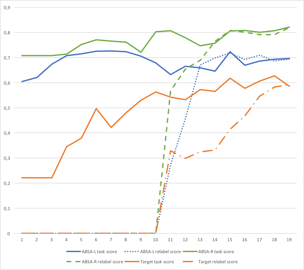
40.4 Label transfer network
To understand the performance of the LTN, we analyse learning curves of the relabelling function vs. the main model. Examples for all tasks without semi-supervised learning are shown in Figure 25. One can observe that the relabelling model does not take long to converge as it has fewer parameters than the main model. Once the relabelling model is learned alongside the main model, the main model performance first stagnates, then starts to increase again. For some of the tasks, the main model ends up with a higher task score than the relabelling model. We hypothesise that the softmax predictions of other, even highly related tasks are less helpful for predicting main labels than the output layer of the main task model. At best, learning the relabelling model alongside the main model might act as a regulariser to the main model and thus improve the main model’s performance over a baseline MTL model, as it is the case for TOPIC-5 (see Table 36).
To further analyse the performance of the LTN, we look into to what degree predictions of the main model and the relabelling model for individual instances are complementary to one another. Or, said differently, we measure the percentage of correct predictions made only by the relabelling model or made only by the main model, relative to the number of correct predictions overall. Results of this for each task are shown in Table 37 for the LTN with and without semi-supervised learning. One can observe that, even though the relabelling function overall contributes to the score to a lesser degree than the main model, a substantial number of correct predictions are made by the relabelling function that are missed by the main model. This is most prominently pronounced for ABSA-R, where the proportion is 14.6.
41 Conclusion
We have presented a multi-task learning architecture that (i) leverages potential synergies between classifier functions relating shared representations with disparate label spaces and (ii) enables learning from mixtures of labeled and unlabeled data. We have presented experiments with combinations of eight pairwise sequence classification tasks. Our results show that leveraging synergies between label spaces sometimes leads to big improvements, and we have presented a new state of the art for topic-based sentiment analysis. Our analysis further showed that (a) the learned label embeddings were indicative of gains from multi-task learning, (b) auxiliary tasks were often beneficial across domains, and (c) label embeddings almost always led to better performance. We also investigated the dynamics of the label transfer network we use for exploiting the synergies between disparate label spaces.
Acknowledgments
Sebastian Ruder is supported by the Irish Research Council Grant Number EBPPG/2014/30 and Science Foundation Ireland Grant Number SFI/12/RC/2289. Anders Søgaard is supported by the ERC Starting Grant Number 313695. Isabelle Augenstein is supported by Eurostars grant Number E10138. We further gratefully acknowledge the support of NVIDIA Corporation with the donation of the Titan Xp GPU used for this research.
7
Sequential Alignment of Text Representations
42 Introduction
As time passes, language usage changes. For example, the names ‘Bert’ and ‘Elmo’ would only rarely make an appearance prior to 2018 in the context of scientific writing. After the publication of BERT (Devlin et al. 2019) and ELMo (Peters et al. 2018), however, usage has increased in frequency. In the context of named entities on Twitter, it is also likely that these names would be tagged as person prior to 2018, and are now more likely to refer to an artefact. As such, their part-of-speech tags will also differ. Evidently, evolution of language usage affects natural language processing (NLP) tasks, and as such, models based on data from one point in time cannot be expected to generalise to the future.
In order to become more robust to language evolution, data should be collected at multiple points in time. We consider a dynamic learning paradigm where one makes predictions for data points from the current time-step given labelled data points from previous time-steps. As time increments, data points from the current step are labelled and new unlabelled data points are observed. This setting occurs in NLP in, for instance, the prediction of paper acceptance to conferences (Kang et al. 2018) or named entity recognition from yearly data dumps of Twitter (Derczynski et al. 2016). Changes in language usage cause a data drift between time-steps and some way of controlling for the shift between time-steps is necessary.
In this paper, we apply a domain adaptation technique to correct for shifts. Domain adaptation is a furtive area of research within machine learning that deals with learning from training data drawn from one data-generating distribution (source domain) and generalising to test data drawn from another, different data-generating distribution (target domain) (Kouw & Loog 2019). We are interested in whether a sequence of adaptations can compensate for the data drift caused by shifts in the meaning of words or features across time. Given that linguistic tokens are embedded in some vector space using neural language models, we observe that in time-varying dynamic tasks, the drift causes token embeddings to occupy different parts of embedding space over consecutive time-steps. We want to avoid the computational expense of re-training a neural network every time-step. Instead, in each time-step, we map linguistic tokens using the same pre-trained language model (a ”BERT” network, Devlin et al. 2019) and align the resulting embeddings using a second procedure called subspace alignment (Fernando et al. 2013). We apply subspace alignment sequentially: find the principal components in each time-step and linearly transform the components from the previous step to match the current step. A classifier trained on the aligned embeddings from the previous step will be more suited to classify embeddings in the current step. We show that sequential subspace alignment (SSA) yields substantial improvements in three challenging tasks: paper acceptance prediction on the PeerRead data set (Kang et al. 2018); Named Entity Recognition on the Broad Twitter Corpus (Derczynski et al. 2016); and rumour stance detection on the RumourEval 2019 data set (Gorrell et al. 2019). These tasks are chosen to vary in terms of domains, timescales, and the granularity of the linguistic units. In addition to evaluating SSA, we include two technical contributions as we extend the method both to allow for time series of unbounded length and to consider instance similarities between classes. The best-performing SSA methods proposed here are semi-supervised, but require only between 2 and 10 annotated data points per class from the test year for successful alignment. Crucially, the best proposed SSA models outperform baselines utilising more data, including the whole data set.
43 Subspace Alignment
Suppose we embed words from a named entity recognition task, where artefacts should be distinguished from persons. Figure 26 shows scatterplots with data collected at two different time-points, say 2017 (top; source domain) and 2018 (bottom; target domain). Red points are examples of artefacts embedded in this space and blue points are examples of persons. We wish to classify the unknown points (black) from 2018 using the labeled points (red/blue bottom) from 2018 and the labeled points from 2017 (red/blue top).
As can be seen, the data from 2017 is not particularly relevant to classification of data from 2018, because the red and blue point clouds do not match. In other words, a classifier trained to discriminate red from blue in 2017 would make a lot of mistakes when applied directly to the data from 2018, partly because words such as ’bert’ have changed from being persons to being artefacts. To make the source data from 2017 relevant – and reap the benefits of having more data – we wish to align source and target data points.
43.1 Unsupervised Subspace Alignment
Unsupervised alignment extracts a set of bases from each data set and transforms the source components such that they match the target components (Fernando et al. 2013). Let be the principal components of the source data and be the components of the target data set . The optimal linear transformation matrix is found by minimising the difference between the transformed source components and the target components:
| (28) |
where denotes the Frobenius norm. Note that we left-multiplied both terms in the norm with the same matrix and that due to orthonormality of the principal components, is the identity and drops out. Source data is aligned to target data by first mapping it onto its own principal components and then applying the transformation matrix, . Target data is also projected onto its target components, . The alignment is performed on the largest principal components, i.e. a subspace of the embedding. Keeping small avoids the high computational expense of eigendecomposition in high-dimensional data.
Unsupervised alignment will only match the total structure of both data sets. Therefore, global shifts between domains can be accounted for, but not local shifts. Figure 26 is an example of a setting with local shifts, i.e. red and blue classes are shifted differently. Performing unsupervised alignment on this setting would fail. Figure 27 (left middle) shows the source data (leftmost) aligned to the target data (rightmost) in an unsupervised fashion. Note that although the total data sets roughly match, the classes (red and blue ellipses) are not matched.
43.2 Semi-Supervised Subspace Alignment
In semi-supervised alignment, one performs subspace alignment per class. As such, at least target label per class needs to be available. However, even then, with only target label per class, we would only be able to find principal component. To allow for the estimation of more components, we provisionally label all target samples using a -nearest-neighbour classifier, starting from the given target labels. Using pseudo-labelled target samples, we estimate components.
Now, the optimal linear transformation matrix for each class can be found with an equivalent procedure as in Equation 28:
| (29) |
Afterwards, we transform the source samples of each class through the projection onto class-specific components and the optimal transformation: . Additionally, we centre each transformed source class on the corresponding target class. Figure 27 (right middle) shows the source documents transformed through semi-supervised alignment. Now, the classes match the target data classes.
43.3 Extending SSA to Unbounded Time
Semi-supervised alignment allows for aligning two time steps, and , to a joint space . However, when considering a further alignment to another time step , this can not trivially be mapped, since the joint space necessarily has a lower dimensionality. Observing that two independently aligned spaces, and , do have the same dimensionality, we further learn a new alignment between the two, resulting in the joint space of and , namely . While there are many ways of joining individual time steps to a single joint space, we approach this by building a binary branching tree, first joining adjacent timesteps with each other, and then joining the new adjacent subspaces with each other.
Although this is seemingly straight-forward, there is no guarantee that and will be coherent with one another, in the same way that two word embedding spaces trained with different algorithms might also differ in spite of having the same dimensionality. This issue is partially taken care of by using semi-supervised alignment which takes class labels into account when learning the ’deeper’ alignment . We further find that it is beneficial to also take the similarities between samples into account when aligning.
43.4 Considering Sample Similarities between Classes
Since intermediary spaces, such as and , do not necessarily share the same semantic properties, we add a step to the semi-supervised alignment procedure. Given that the initial unaligned spaces do encode similarities between instances, we run the -means clustering algorithm () to give us some course-grained indication of instance similarities in the original embedding space. This cluster ID is passed to SSA, resulting in an alignment which both attempts to match classes across time steps, in addition to instance similarities. Hence, even though and are not necessarily semantically coherent, an alignment to is made possible.
44 Experimental Setup
In the past year, several approaches to pre-training representations on language modelling based on transformer architectures (Vaswani et al. 2017) have been proposed. These models essentially use a multi-head self-attention mechanism in order to learn representations which are able to attend directly to any part of a sequence. Recent work has shown that such contextualised representations pre-trained on language modelling tasks offer highly versatile representations which can be fine-tuned on seemingly any given task (Peters et al. 2018; Devlin et al. 2019; Radford et al. 2018; Radford et al. 2019a). In line with the recommendations from experiments on fine-tuning representations (Peters et al. 2019), we use a frozen BERT to extract a consistent task-agnostic representation. Using a frozen BERT with subsequent subspace alignment allows us to avoid re-training a neural network each time-step while still working in an embedding learned by a neural language model. It also allows us to test the effectiveness of SSA without the confounding influence of representation updates.
Three Tasks.
We consider three tasks representing a broad selection of natural language understanding scenarios: paper acceptance prediction based on the PeerRead data set (Kang et al. 2018), Named Entity Recognition (NER) based on the Broad Twitter Corpus (Derczynski et al. 2016), and author stance prediction based on the RumourEval-2019 data set (Gorrell et al. 2019). These tasks were chosen so as to represent i) different textual domains, across ii) differing time scales, and iii) operating at varying levels of linguistic granularity. As we are dealing with dynamical learning, the vast majority of NLP data sets can unfortunately not be used since they do not include time stamps.
45 Paper Acceptance Prediction
| Test year | All | Same | Prev | Unsup. | Semi-sup. | Unsup. Unb. | S. Unb. | S. Unb. w/Clst |
|---|---|---|---|---|---|---|---|---|
| 2010 | 61.77 | 67.64 | 35.29 | 70.59 | 70.59 | 70.58 | 70.59 | 70.59 |
| 2011 | 61.77 | 58.82 | 55.88 | 14.71 | 72.35 | 24.71 | 72.35 | 72.35 |
| 2012 | 56.25 | 56.25 | 58.75 | 50.00 | 72.50 | 45.00 | 72.80 | 72.30 |
| 2013 | 67.54 | 56.14 | 58.78 | 76.31 | 78.07 | 72.31 | 78.97 | 79.03 |
| 2014 | 50.53 | 51.64 | 51.64 | 36.88 | 68.03 | 31.88 | 69.03 | 69.45 |
| 2015 | 57.83 | 54.05 | 54.05 | 49.19 | 58.37 | 41.19 | 59.97 | 59.93 |
| 2016 | 58.89 | 57.36 | 57.36 | 50.61 | 61.04 | 38.61 | 63.04 | 63.04 |
| 2017 | 56.04 | 58.24 | 58.24 | 68.13 | 63.73 | 58.13 | 68.73 | 69.80 |
| avg | 58.82 | 57.52 | 53.75 | 52.05 | 68.09 | 47.80 | 69.44 | 69.56 |
The PeerRead data set contains papers from ten years of arXiv history, as well as papers and reviews from major AI and NLP conferences (Kang et al. 2018).3030 30 https://github.com/allenai/PeerRead From the perspective of evaluating our method, the arXiv sub-set of this data set offers the possibility of evaluating our method while adapting to ten years of history. This is furthermore the only subset of the data annotated with both timestamps and with a relatively balanced accept/reject annotation.3131 31 The NIPS selection, ranging from 2013-2017, only contains accepted papers. The other conferences contain accept/reject annotation, but only represent single years. As arXiv naturally contains both accepted and rejected papers, this acceptance status has been assigned based on Sutton & Gong 2017 who match arXiv submissions to bibliographic entries in DBLP, and additionally defining acceptance as having been accepted to major conferences, and not to workshops. This results in a data set of nearly 12,000 papers, from which we use the raw abstract text as input to our system. The first three years were filtered out due to containing very few papers. We use the standard train/test splits supplied with the data set.
Kang et al. 2018 show that it is possible to predict paper acceptance status at major conferences at above baseline levels. Our intuition in applying SSA to this problem, is that the topic of a paper is likely to bias acceptance to certain conferences across time. For instance, it is plausible that the likelihood of a neural paper being accepted to an NLP conference before and after 2013 differs wildly. Hence, we expect that our model will, to some extent, represent the topic of an article, and that this will lend itself nicely to SSA.
45.1 Model
We use the pre-trained bert-base-uncased model as the base for our paper acceptance prediction model. Following the approach of Devlin et al. 2019, we take the final hidden state (i.e., the output of the transformer) corresponding to the special [CLS] token of an input sequence to be our representation of a paper, as this has aggregated information through the sequence (Figure 28). This gives us a -dimensional representation of each document, where . In all of the experiments for this task, we train an SVM with an RBF kernel on these representations, either with or without SSA depending on the setting.

45.2 Experiments & Results
We set up a series of experiments where we observe past data, and evaluate on present data. We compare both unsupervised and semi-supervised subspace alignment, with several strong baselines. The baselines represent cases in which we have access to more data, and consist of training our model on either all data (i.e. both past and future data), on the same year as the evaluation year, and on the previous year. In our alignment settings, we only observe data from the previous year, and apply subspace alignment. This is a different task than presented by Kang et al. 2018, as we evaluate paper acceptance for papers in the present. Hence, our scores are not directly comparable to theirs.
One parameter which significantly influences performance, is the number of labelled data points we use for learning the semi-supervised subspace alignment. We tuned this hyperparameter on the development set, finding an increasing trend. Using as few as 2 tuning points per class yielded an increase in performance in some cases (Figure 29).

Our results are shown in Table 38, using 10 tuning samples per class. With unsupervised subspace alignment, we observe relatively unstable results – in one exceptional case, namely testing on 2010, unsupervised alignment is as helpful as semi-supervised alignment. Semi-supervised alignment, however, yields consistent improvements in performance across the board. It is especially promising that adapting from past data outperforms training on all available data, as well as training on the actual in-domain data. This highlights the importance of controlling for data drift due to language evolution. It shows that this signal can be taken advantage of to increase performance on present data with only a small amount of annotated data. We further find that using several past time steps in the Unbounded condition is generally helpful, as is using instance similarities in the alignment.
46 Named Entity Recognition
| Test year | All | Same | Prev | Unsup. | Semi-sup. | Unsup. Unb. | S. Unb. | S. Unb. w/Clst |
|---|---|---|---|---|---|---|---|---|
| 2013 | 62.95 | 42.24 | 54.16 | 42.25 | 63.82 | 42.25 | 63.82 | 63.95 |
| 2014 | 72.77 | 77.76 | 59.53 | 50.43 | 73.67 | 50.43 | 73.67 | 78.75 |
| avg | 67.86 | 60.00 | 56.85 | 46.34 | 68.75 | 46.34 | 68.75 | 71.35 |
The Broad Twitter Corpus contains tweets annotated with named entities, collected between the years 2009 and 2014 (Derczynski et al. 2016). However, as only a handful of tweets are collected before 2012, we focus our analysis on the final three years of this period (i.e. two test years). The corpus includes diverse data, annotated in part via crowdsourcing and in part by experts. The inventory of tags in their tag scheme is relatively small, including Person, Location, and Organisation. To the best of our knowledge no one has evaluated on this corpus either in general or per year, and so we cannot compare with previous work.
In the case of NER, we expect the adaptation step of our model to capture the fact that named entities may change their meaning across time (e.g. the example with “Bert” and “BERT” in Figure 26). This is related to work showing temporal drift of topics (Wang & McCallum 2006).
46.1 Model
Since casing is typically an important feature in NER, we use the pre-trained bert-base-cased model as our base for NER. For each token, we extract its contextualised representation from BERT, before applying SSA. As Devlin et al. 2019 achieve state-of-the-art results without conditioning the predicted tag sequence on surrounding tags (as would be the case with a CRF, for example), we also opt for this simpler architecture. The resulting contextualised representations are therefore passed to an MLP with a single hidden layer (200 hidden units, ReLU activation), before predicting NER tags. We train the MLP over 5 epochs using the Adam optimiser (Kingma & Ba 2015).
46.2 Experiments & Results
As with previous experiments, we compare unsupervised and semi-supervised subspace alignment with baselines corresponding to using all data, data from the same year as the evaluation year, and data from the previous year. For each year, we divide the data into 80/10/10 splits for training, development, and test. Results on the two test years 2013 and 2014 are shown in Table 39. In the case of NER, we do not observe any positive results for unsupervised subspace alignment. In the case of semi-supervised alignment, however, we find increased performance as compared to training on the previous year, and compared to training on all data. This shows that learning an alignment from just a few data points can help the model to generalise from past data. However, unlike our previous experiments, results are somewhat better when given access to the entire set of training data from the test year itself in the case of NER. The fact that training on only 2013 and evaluating on the same year does not work well can be explained by the fact that the amount of data available for 2013 is only 10% of that for 2012. The identical results for the unbounded extension is because aligning from a single time step renders this irrelevant.
47 SDQC Stance Classification
The RumourEval-2019 data set consists of roughly 5500 tweets collected for 8 events surrounding well-known incidents, such as the Charlie Hebdo shooting in Paris (Gorrell et al. 2019).3232 32 http://alt.qcri.org/semeval2019/index.php?id=tasks Since the shared task test set is not available, we split the training set into a training, dev and test part based on rumours (one rumour will be training data with a 90/10 split for development and another rumour will be the test data, with a few samples labelled). For Subtask A, tweets are annotated with stances, denoting whether it is in the category Support, Deny, Query, or Comment (SDQC).
Each rumour only lasts a couple of days, but the total data set spans years, from August 2014 to November 2016. We regard each rumour as a time-step and adapt from the rumour at time - to the rumour at time . We note that this setting is more difficult than the previous two due to the irregular time intervals. We disregard the rumour ebola-essien as it has too few samples per class.
47.1 Model
For this task, we use the same modelling approach as described for paper acceptance prediction. This method is also suitable here, since we simply require a condensed representation of a few sentences on which to base our temporal adaptation and predictions. In the last iteration of the task, the winning system used hand-crafted features to achieve a high performance (Kochkina et al. 2017). Including these would complicate SSA, so we opt for this simpler architecture instead. We use the shorter time-scale of approximately weeks rather than years as rumours can change rapidly (Kwon et al. 2017).
47.2 Experiments & Results
In this experiment, we start with the earliest rumour and adapt to the next rumour in time. As before, we run the following baselines: training on all available labelled data (i.e. all previous rumours and the labelled data for the current rumour), training on the labelled data from the current rumour (designated as ‘same’) and training on the labelled data from the previous rumour. We perform both unsupervised and semi-supervised alignment using data from the previous rumour. We label 5 samples per class for each rumour.
In this data set, there is a large class imbalance, with a large majority of comment tweets and few support or deny tweets. To address this, we over-sample the minority classes. Afterwards, a SVM with RBF is trained and we test on unlabelled tweets for the current rumour. Table 40 shows the performance of the baselines and the two alignment procedures. As with the previous tasks, semi-supervised alignment generally helps, except for in the charliehebdo rumour.
| Test year | All | Same | Prev | Unsup. | Semi-sup. | Unsup. Unb. | S. Unb. | S. Unb. w/Clst |
|---|---|---|---|---|---|---|---|---|
| ottawashooting | 31.51 | 23.67 | 30.77 | 30.77 | 31.88 | 28.37 | 30.68 | 30.88 |
| prince-toronto | 36.27 | 23.37 | 34.46 | 34.46 | 40.32 | 31.36 | 39.12 | 39.52 |
| sydney-siege | 32.34 | 27.17 | 41.23 | 41.23 | 43.60 | 33.23 | 43.50 | 43.54 |
| charliehebdo | 38.51 | 31.67 | 35.73 | 35.73 | 33.76 | 33.71 | 32.70 | 32.61 |
| putinmissing | 28.33 | 22.38 | 34.53 | 34.53 | 36.11 | 31.95 | 35.10 | 35.81 |
| germanwings-crash | 29.38 | 22.01 | 44.79 | 44.79 | 44.84 | 40.30 | 44.88 | 44.80 |
| illary | 29.24 | 25.81 | 37.53 | 37.53 | 40.08 | 34.10 | 39.30 | 38.95 |
| avg | 31.13 | 25.16 | 37.00 | 37.00 | 38.65 | 33.29 | 37.90 | 38.02 |
48 Analysis and Discussion
We have shown that sequential subspace alignment is useful across natural language processing tasks. For the PeerRead data set we were particularly successful. This might be explained by the fact that the topic of a paper is a simple feature for SSA to pick up on, while being predictive of a paper’s acceptance chances. For NER, on the other hand, named entities can change in less predictable ways across time, proving a larger challenge for our approach. For SDQC, we were successful in cases where the tweets are nicely clustered by class. For instance, where both rumours are about terrorist attacks, many of the support tweets were headlines from reputable newspaper agencies. These agencies structure tweets in a way that is consistently dissimilar from comments and queries.
The effect of our unbounded time extension boosts results on the PeerRead data set, as the data stretches across a range of years. In the case of NER, however, this extension is excessive as only two time steps are available. In the case of SDQC, the lack of improvement could be due to the irregular time intervals, making it hard to learn consistent mappings from rumour to rumour. Adding instance similarity clustering aids alignment, since considering sample similarities across classes is important over longer time scales.
48.1 Example of Aligning Tweets
Finally, we set up the following simplified experiment to investigate the effect of alignment on SDQC data. First, we consider the rumour charliehebdo, where we picked the following tweet:
Support:
France: 10 people dead after shooting at HQ of satirical weekly newspaper #CharlieHebdo, according to witnesses <URL>
It has been labeled to be in support of the veracity of the rumour. We will consider the scenario where we use this tweet and others involving the charliehebdo incident to predict author stance in the rumour germanwings-crash. Before alignment, the following 2 germanwings-crash tweets are among the nearest neighbours in the embedding space:
Query:
@USER @USER if they had, it’s likely the descent rate would’ve been steeper and the speed not reduce, no ?
Comment:
@USER Praying for the families and friends of those involved in crash. I’m so sorry for your loss.
The second tweet is semantically similar (both are on the topic of tragedy), but the other is unrelated. Note that the news agency tweet differs from the comment and query tweets in that it stems from a reputable source, mentions details and includes a reference. After alignment, the charliehebdo tweet has the following 2 nearest neighbours:
Support:
“@USER: 148 passengers were on board #GermanWings Airbus A320 which has crashed in the southern French Alps <URL>”
Support:
Report: Co-Pilot Locked Out Of Cockpit Before Fatal Plane Crash <URL> #Germanwings <URL>
Now, both neighbours are of the support class. This example shows that semi-supervised alignment maps source tweets from one class close to target tweets of the same class.
48.2 Limitations
A necessary assumption in subspace alignment is that classes are clustered in the embedding space: most embedded tokens should lie closer to other embedded tokens of the same class than to embedded tokens of another class. If this is not the case, then aligning based on a few labelled samples of class does not imply that the embedded source tokens are aligned to other target points of class . This assumption is violated if, for instance, people only discuss one aspect of a rumour on day one and discuss several aspects of a rumour simultaneously on day two. One would observe a single cluster of token embeddings for supporters of the rumour initially and several clusters at a later time-step. Note that there is no unique solution for aligning a single cluster to multiple clusters.
Additionally, if those few samples labeled in the current time-step (for semi-supervised alignment) are falsely labeled or their label is ambiguous (e.g. a tweet that could equally be labeled as query or deny), then the source data could be aligned to the wrong point cloud. It is important that the few labeled tokens actually represent their classes. This is a common requirement in semi-supervised learning and is not specific to sequential alignment of text representations.
48.3 Related Work
The temporal nature of data can have a significant impact in natural language processing tasks. For instance, Kutuzov et al. 2018 compare a number of approaches to diachronic word embeddings, and detection of semantic shifts across time. For instance, such representations can be used to uncover changes of word meanings, or senses of new words altogether (Gulordava & Baroni 2011; Heyer et al. 2009; Michel et al. 2011; Mitra et al. 2014; Wijaya & Yeniterzi 2011). Other work has investigated changes in the usage of parts of speech across time (Mihalcea & Nastase 2012). Yao et al. 2018 investigate the changing meanings and associations of words across time, in the perspective of language change. By learning time-aware embeddings, they are able to outperform standard word representation learning algorithms, and can discover, e.g., equivalent technologies through time. Lukeš & Søgaard 2018 show that lexical features can change their polarity across time, which can have a significant impact in sentiment analysis. Wang & McCallum 2006 show that associating topics with continuous distributions of timestamps yields substantial improvements in terms of topic prediction and interpretation of trends. Temporal effects in NLP have also been studied in the context of scientific journals, for instance in the context of emerging themes and viewpoints (Blei & Lafferty 2006; Sipos et al. 2012), and in terms of topic modelling on news corpora across time (Allan et al. 2001). Finally, in the context of rumour stance classification, Lukasik et al. 2016a show that temporal information as a feature in addition to textual content offers an improvement in results. While this previous work has highlighted the extent to which language change across time is relevant for NLP, we present a concrete approach to taking advantage of this change. Nonetheless, these results could inspire more specialised forms of sequential adaptation for specific tasks.
Unsupervised subspace alignment has been used in computer vision to adapt between various types of representations of objects, such as high-definition photos, online retail images and illustrations (Fernando et al. 2013). Alignment is not restricted to linear transformations, but can be made non-linear through kernelisation (Aljundi et al. 2015). An extension to semi-supervised alignment has been done for images (Yao et al. 2015), but not in the context of classification of text embeddings or domain adaptation on a sequential basis.
49 Conclusions
In this paper, we introduced sequential subspace alignment (SSA) for natural language processing (NLP), which allows for improved generalisation from past to present data. Experimental evidence shows that this method is useful across diverse NLP tasks, in various temporal settings ranging from weeks to years, and for word-level and document-level representations. The best-performing SSA method, aligning sub-spaces in a semi-supervised way, outperforms simply training on all data with no alignment.
Acknowledgements
WMK was supported by the Niels Stensen Fellowship.
8
A Diagnostic Study of Explainability Techniques
50 Introduction
Understanding the rationales behind models’ decisions is becoming a topic of pivotal importance, as both the architectural complexity of machine learning models and the number of their application domains increases. Having greater insight into the models’ reasons for making a particular prediction has already proven to be essential for discovering potential flaws or biases in medical diagnosis (Caruana et al. 2015) and judicial sentencing (Rich 2016). In addition, European law has mandated “the right to obtain an explanation of the decision reached” (Regulation 2016).
Explainability methods attempt to reveal the reasons behind a model’s prediction for a single data point, as shown in Figure 30. They can be produced post-hoc, i.e., with already trained models. Such post-hoc explanation techniques can be applicable to one specific model (Martens et al. 2008; Wagner et al. 2019) or to a broader range thereof (Ribeiro et al. 2016; Lundberg & Lee 2017). They can further be categorised as: employing model gradients (Sundararajan et al. 2017; Simonyan et al. 2014), being perturbation based (Shapley 1953; Zeiler & Fergus 2014) or providing explanations through model simplifications (Ribeiro et al. 2016; Johansson et al. 2004). There also exist explainability methods that generate textual explanations (Camburu et al. 2018) and are trained post-hoc or jointly with the model at hand.
While there is a growing amount of explainability methods, we find that they can produce varying, sometimes contradicting explanations, as illustrated in Figure 30. Hence, it is important to assess existing techniques and to provide a generally applicable and automated methodology for choosing one that is suitable for a particular model architecture and application task (Jacovi & Goldberg 2020). Robnik-Sikonja & Bohanec 2018 compiles a list of property definitions for explainability techniques, but it remains a challenge to evaluate them in practice. Several other studies have independently proposed different setups for probing varied aspects of explainability techniques (DeYoung et al. 2020; Sundararajan et al. 2017). However, existing studies evaluating explainability methods are discordant and do not compare to properties from previous studies. In our work, we consider properties from related work and extend them to be applicable to a broader range of downstream tasks.
Furthermore, to create a thorough setup for evaluating explainability methods, one should include at least: (i) different groups of explainability methods (explanation by simplification, gradient-based, etc.), (ii) different downstream tasks, and (iii) different model architectures. However, existing studies usually consider at most two of these aspects, thus providing insights tied to a specific setup.
We propose a number of diagnostic properties for explainability methods and evaluate them in a comparative study. We consider explainability methods from different groups, all widely applicable to most ML models and application tasks. We conduct an evaluation on three text classification tasks, which contain human annotations of salient tokens. Such annotations are available for Natural Language Processing (NLP) tasks, as they are relatively easy to obtain. This is in contrast to ML sub-fields such as image analysis, for which we only found one relevant dataset – 536 manually annotated object bounding boxes for Visual Question Answering (Subramanian et al. 2020).
We further compare explainability methods across three of the most widely used model architectures – , , and . The model achieves state-of-the-art performance on many text classification tasks but has a complex architecture, hence methods to explain its predictions are strongly desirable. The proposed properties can also be directly applied to Machine Learning (ML) subfields other than NLP. The code for the paper is publicly available.3333
33
https://github.com/copenlu/xai-benchmark
In summary, the contributions of this work are:
- •
We compile a comprehensive list of diagnostic properties for explainability and automatic measurement of them, allowing for their effective assessment in practice.
- •
We study and compare the characteristics of different groups of explainability techniques in three different application tasks and three different model architectures.
- •
We study the attributions of the explainability techniques and human annotations of salient regions to compare and contrast the rationales of humans and machine learning models.
51 Related Work
Explainability methods can be divided into explanations by simplification, e.g., LIME (Ribeiro et al. 2016); gradient-based explanations (Sundararajan et al. 2017); perturbation-based explanations (Shapley 1953; Zeiler & Fergus 2014). Some studies propose the generation of text serving as an explanation, e.g., Camburu et al. 2018; Lei et al. 2016; Atanasova et al. 2020a. For extensive overviews of existing explainability approaches, see Arrieta et al. 2020.
Explainability methods provide explanations of different qualities, so assessing them systematically is pivotal. A common attempt to reveal shortcomings in explainability techniques is to reveal a model’s reasoning process with counter-examples (Alvarez-Melis & Jaakkola 2018; Kindermans et al. 2019; Atanasova et al. 2020b), finding different explanations for the same output. However, single counter-examples do not provide a measure to evaluate explainability techniques (Jacovi & Goldberg 2020).
Another group of studies performs human evaluation of the outputs of explainability methods (Lertvittayakumjorn & Toni 2019; Narayanan et al. 2018). Such studies exhibit low inter-annotator agreement and reflect mostly what appears to be reasonable and appealing to the annotators, not the actual properties of the method.
The most related studies to our work design measures and properties of explainability techniques. Robnik-Sikonja & Bohanec 2018 propose an extensive list of properties. The Consistency property captures the difference between explanations of different models that produce the same prediction; and the Stability property measures the difference between the explanations of similar instances given a single model. We note that similar predictions can still stem from different reasoning paths. Instead, we propose to explore instance activations, which reveal more of the model’s reasoning process than just the final prediction. The authors propose other properties as well, which we find challenging to apply in practice. We construct a comprehensive list of diagnostic properties tied with measures that assess the degree of each characteristic.
Another common approach to evaluate explainability methods is to measure the sufficiency of the most salient tokens for predicting the target label (DeYoung et al. 2020). We also include a sufficiency estimate, but instead of fixing a threshold for the tokens to be removed, we measure the decrease of a model’s performance, varying the proportion of excluded tokens. Other perturbation-based evaluation studies and measures exist (Sundararajan et al. 2017; Adebayo et al. 2018), but we consider the above, as it is the most widely applied.
Another direction of explainability evaluation is to compare the agreement of salient words annotated by humans to the saliency scores assigned by explanation techniques (DeYoung et al. 2020). We also consider the latter and further study the agreement across model architectures, downstream tasks, and explainability methods. While we consider human annotations at the word level (Camburu et al. 2018; Lei et al. 2016), there are also datasets (Clark et al. 2019; Khashabi et al. 2018) with annotations at the sentence-level, which would require other model architectures, so we leave this for future work.
Existing studies for evaluating explainability heavily differ in their scope. Some concentrate on a single model architecture - BERT-LSTM (DeYoung et al. 2020), RNN (Arras et al. 2019), CNN (Lertvittayakumjorn & Toni 2019), whereas a few consider more than one model (Guan et al. 2019; Poerner et al. 2018). Some studies concentrate on one particular dataset (Guan et al. 2019; Arras et al. 2019), while only a few generalize their findings over downstream tasks (DeYoung et al. 2020; Vashishth et al. 2019). Finally, existing studies focus on one (Vashishth et al. 2019) or a single group of explainability methods (DeYoung et al. 2020; Adebayo et al. 2018). Our study is the first to propose a unified comparison of different groups of explainability techniques across three text classification tasks and three model architectures.
52 Evaluating Attribution Maps
We now define a set of diagnostic properties of explainability techniques, and propose how to quantify them. Similar notions can be found in related work (Robnik-Sikonja & Bohanec 2018; DeYoung et al. 2020), and we extend them to be generally applicable to downstream tasks. We first introduce the prerequisite notation. Let be the test dataset, where each instance consists of a list of tokens = , a gold label , and a gold saliency score for each of the tokens in : with each . Let be an explanation technique that, given a model , a class , and a single instance , computes saliency scores for each token in the input: . Finally, let be models with the same architecture, each trained from a randomly chosen seed, and let be models of the same architecture, but with randomly initialized weights.
Agreement with human rationales (HA). This diagnostic property measures the degree of overlap between saliency scores provided by human annotators, specific to the particular task, and the word saliency scores computed by an explainability technique on each instance. The property is a simple way of approximating the quality of the produced feature attributions. While it does not necessarily mean that the saliency scores explain the predictions of a model, we assume that explanations with high agreement scores would be more comprehensible for the end-user as they would adhere more to human reasoning. With this diagnostic property, we can also compare how the type and the performance of a model and/or dataset affect the agreement with human rationales when observing one type of explainability technique.
During evaluation, we provide an estimate of the average agreement of the explainability technique across the dataset. To this end, we start at the instance level and compute the Average Precision (AP) of produced saliency scores by comparing them to the gold saliency annotations . Here, the label for computing the saliency scores is the gold label: . Then, we compute the average across all instances, arriving at Mean AP (MAP):
| (30) |
Confidence Indication (CI). A token from a single instance can receive several saliency scores, indicating its contribution to the prediction of each of the classes. Thus, when a model recognizes a highly indicative pattern of the predicted class , the tokens involved in the pattern would have highly positive saliency scores for this class and highly negative saliency scores for the remaining classes. On the other hand, when the model is not highly confident, we can assume that it is unable to recognize a strong indication of any class, and the tokens accordingly do not have high saliency scores for any class. Thus, the computed explanation of an instance should indicate the confidence of the model in its prediction.
We propose to measure the predictive power of the produced explanations for the confidence of the model. We start by computing the Saliency Distance (SD) between the saliency scores for the predicted class to the saliency scores of the other classes (Eq. 31). Given the distance between the saliency scores, we predict the confidence of the class with logistic regression (LR) and finally compute the Mean Absolute Error – MAE (Eq. 32), of the predicted confidence to the actual one.
| (31) | |||
| (32) |
For tasks with two classes, D is the subtraction of the saliency value for class k and the other class. For more than two classes, D is the concatenation of the max, min, and average across the differences of the saliency value for class k and the other classes. Low MAE indicates that model’s confidence can be easily identified by looking at the produced explanations.
Faithfulness (F). Since explanation techniques are employed to explain model predictions for a single instance, an essential property is that they are faithful to the model’s inner workings and not based on arbitrary choices. A well-established way of measuring this property is by replacing a number of the most-salient words with a mask token (DeYoung et al. 2020) and observing the drop in the model’s performance. To avoid choosing an unjustified percentage of words to be perturbed, we produce several dataset perturbations by masking 0, 10, 20, …, 100% of the tokens in order of decreasing saliency, thus arriving at , , …, . Finally, to produce a single number to measure faithfulness, we compute the area under the threshold-performance curve (AUC-TP):
| (33) | |||
where P is a task specific performance measure and . We also compare the AUC-TP of the saliency methods to a random saliency map to find whether there are explanation techniques producing saliency scores without any contribution over a random score.
Using AUC-TP, we perform an ablation analysis which is a good approximation of whether the most salient words are also the most important ones for a model’s prediction. However, some prior studies (Feng et al. 2018) find that models remain confident about their prediction even after stripping most input tokens, leaving a few that might appear nonsensical to humans. The diagnostic properties that follow aim to facilitate a more in-depth analysis of the alignment between the inner workings of a model and produced saliency maps.
Rationale Consistency (RC). A desirable property of an explainability technique is to be consistent with the similarities in the reasoning paths of several models on a single instance. Thus, when two reasoning paths are similar, the scores provided by an explainability technique should also be similar, and vice versa. Note that we are interested in similar reasoning paths as opposed to similar predictions, as the latter does not guarantee analogous model rationales. For models with diverse architectures, we expect rationales to be diverse as well and to cause low consistency. Therefore, we focus on a set of models with the same architecture, trained from different random seeds as well as the same architecture, but with randomly initialized weights. The latter would ensure that we can have model pairs with similar and distant rationales. We further claim that the similarity in the reasoning paths could be measured effectively with the distance between the activation maps (averaged across layers and neural nodes) produced by two distinct models (Eq. 34). The distance between the explanation scores is computed simply by subtracting the two (Eq. 35). Finally, we compute Spearman’s between the similarity of the explanation scores and the similarity of the attribution maps (Eq. 36).
| (34) | |||
| (35) | |||
| (36) |
The higher the positive correlation is, the more consistent the attribution method would be. We choose Spearman’s as it measures the monotonic correlation between the two variables. On the other hand, Pearson’s measures only the linear correlation, and we can have a non-linear correlation between the activation difference and the saliency score differences. When subtracting saliency scores and layer activations, we also take the absolute value of the vector difference as the property should be invariant to order of subtraction. An additional benefit of the property is that low correlation scores would also help to identify explainability techniques that are not faithful to a model’s rationales.
Dataset Consistency (DC). The next diagnostic property is similar to the above notion of rationale consistency but focuses on consistency across instances of a dataset as opposed to consistency across different models of the same architecture. In this case, we test whether instances with similar rationales also receive similar explanations. While Rationale Consistency compares instance explanations of the same instance for different model rationales, Dataset Consistency compares explanations for pairs of instances on the same model. We again measure the similarity between instances and by comparing their activation maps, as in Eq. 37. The next step is to measure the similarity of the explanations produced by an explainability technique , which is the difference between the saliency scores as in Eq. 38. Finally, we measure Spearman’s between the similarity in the activations and the saliency scores as in Eq. 39. We again take the absolute value of the difference.
| (37) | |||
| (38) | |||
| (39) |
53 Experiments
53.1 Datasets
| Dataset | Example | Size | Length |
|---|---|---|---|
|
e-SNLI
Camburu et al. 2018 |
Premise: An adult dressed in black holds a stick.
Hypothesis: An adult is walking away, empty-handed. Label: contradiction |
549 367 Train
9 842 Dev 9 824 Test |
27.4 inst.
5.3 expl. |
|
Movie
Reviews Zaidan et al. 2007 |
Review: he is one of the most exciting martial artists on the big screen, continuing to perform his own stunts and dazzling audiences with his flashy kicks and punches.
Class: Positive |
1 399 Train
199 Dev 199 Test |
834.9 inst.
56.18 expl. |
|
Tweet
Sentiment Extraction (TSE) 3434 34 https://www.kaggle.com/c/tweet-sentiment-extraction |
Tweet: im soo bored…im deffo missing my music channels
Class: Negative |
21 983 Train
2 747 Dev 2 748 Test |
20.5 inst.
9.99 expl. |
Table 41 provides an overview of the used datasets. For e-SNLI, models predict inference – contradiction, neutral, or entailment – between sentence tuples. For the Movie Reviews dataset, models predict the sentiment – positive, negative, or neutral – of reviews with multiple sentences. Finally, for the TSE dataset, models predict tweets’ sentiment – positive, negative, or neutral. The e-SNLI dataset provides three dataset splits with human-annotated rationales, which we use as training, dev, and test sets, respectively. The Movie Reviews dataset provides rationale annotations for nine out of ten splits. Hence, we use the ninth split as a test and the eighth split as a dev set, while the rest are used for training. Finally, the TSE dataset only provides rationale annotations for the training dataset, and we therefore randomly split it into 80/10/10% chunks for training, development and testing.
53.2 Models
| Model | Val | Test |
|---|---|---|
| e-SNLI | ||
| 0.897 (0.002) | 0.892 () | |
| 0.167 (0.003) | 0.167 () | |
| 0.773 (0.003) | 0.768 () | |
| 0.195 () | 0.194 () | |
| 0.794 (0.005) | 0.793 () | |
| 0.176 () | 0.176 () | |
| Movie Reviews | ||
| 0.859 (0.044) | 0.856 (0.018) | |
| 0.335 (0.003) | 0.333 () | |
| 0.831 (0.014) | 0.773 (0.005) | |
| 0.343 (0.020) | 0.333 () | |
| 0.614 (0.017) | 0.567 () | |
| 0.362 (0.030) | 0.363 () | |
| TSE | ||
| 0.772 (0.005) | 0.781 () | |
| 0.165 (0.025) | 0.171 () | |
| 0.708 (0.007) | 0.730 () | |
| 0.221 (0.060) | 0.226 () | |
| 0.701 (0.005) | 0.727 () | |
| 0.196 (0.070) | 0.204 () | |
We experiment with different commonly used base models, namely (Fukushima 1980), (Hochreiter & Schmidhuber 1997), and the (Vaswani et al. 2017) architecture BERT (Devlin et al. 2019). The selected models allow for a comparison of the explainability techniques on diverse model architectures. Table 44 presents the performance of the separate models on the datasets.
For the model, we use an embedding, a convolutional, a max-pooling, and a linear layer. The embedding layer is initialized with GloVe (Pennington et al. 2014) embeddings and is followed by a dropout layer. The convolutional layer computes convolutions with several window sizes and multiple-output channels with ReLU (Hahnloser et al. 2000) as an activation function. The result is compressed down with a max-pooling layer, passed through a dropout layer, and into a fine linear layer responsible for the prediction. The final layer has a size equal to the number of classes in the dataset.
The model again contains an embedding layer initialized with the GloVe embeddings. The embeddings are passed through several bidirectional LSTM layers. The final output of the recurrent layers is passed through three linear layers and a final dropout layer.
For the model, we fine-tune the pre-trained basic, uncased language model (LM) (Wolf et al. 2019). The fine-tuning is performed with a linear layer on top of the LM with a size equal to the number of classes in the corresponding task. Further implementation details for all of the models, as well as their F1 scores, are presented in 56.1.
53.3 Explainability Techniques
We select the explainability techniques to be representative of different groups – gradient (Sundararajan et al. 2017; Simonyan et al. 2014), perturbation (Shapley 1953; Zeiler & Fergus 2014) and simplification based (Ribeiro et al. 2016; Johansson et al. 2004).
Starting with the gradient-based approaches, we select Saliency (Simonyan et al. 2014) as many other gradient-based explainability methods build on it. It computes the gradient of the output w.r.t. the input. We also select two widely used improvements of the Saliency technique, namely InputXGradient (Kindermans et al. 2016), and Guided Backpropagation (Springenberg et al. 2015). InputXGradient additionally multiplies the gradient with the input and Guided Backpropagation overwrites the gradients of ReLU functions so that only non-negative gradients are backpropagated.
From the perturbation-based approaches, we employ Occlusion (Zeiler & Fergus 2014), which replaces each token with a baseline token (as per standard, we use the value zero) and measures the change in the output. Another popular perturbation-based technique is the Shapley Value Sampling (Castro et al. 2009). It is based on the Shapley Values approach that computes the average marginal contribution of each word across all possible word perturbations. The Sampling variant allows for a faster approximation of Shapley Values by considering only a fixed number of random perturbations as opposed to all possible perturbations.
Finally, we select the simplification-based explanation technique LIME (Ribeiro et al. 2016). For each instance in the dataset, LIME trains a linear model to approximate the local decision boundary for that instance.
Generating explanations. The saliency scores from each of the explainability methods are generated for each of the classes in the dataset. As all of the gradient approaches provide saliency scores for the embedding layer (the last layer that we can compute the gradient for), we have to aggregate them to arrive at one saliency score per input token. As we found different aggregation approaches in related studies (Bansal et al. 2016; DeYoung et al. 2020), we employ the two most common methods – L2 norm and averaging (denoted as and in the explainability method names).
54 Results and Discussion
We report the measures of each diagnostic property as well as FLOPs as a measure of the computing time used by the particular method. For all diagnostic properties, we also include the randomly assigned saliency as a baseline.
54.1 Results
| Saliency | e-SNLI | IMDB | TSE |
|---|---|---|---|
| Random | 0.201 | 0.517 | 0.185 |
| ShapSampl | 0.479 | 0.481 | 0.667 |
| LIME | 0.809 | 0.604 | 0.553 |
| Occlusion | 0.523 | 0.323 | 0.556 |
| 0.772 | 0.671 | 0.707 | |
| 0.781 | 0.687 | 0.696 | |
| 0.364 | 0.432 | 0.307 | |
| 0.796 | 0.676 | 0.754 | |
| 0.468 | 0.236 | 0.287 | |
| 0.782 | 0.676 | 0.685 | |
| Random | 0.209 | 0.468 | 0.384 |
| ShapSampl | 0.460 | 0.648 | 0.630 |
| LIME | 0.571 | 0.572 | 0.681 |
| Occlusion | 0.554 | 0.411 | 0.594 |
| 0.853 | 0.712 | 0.595 | |
| 0.875 | 0.796 | 0.631 | |
| 0.576 | 0.662 | 0.613 | |
| 0.881 | 0.759 | 0.636 | |
| 0.403 | 0.346 | 0.438 | |
| 0.875 | 0.788 | 0.628 | |
| Random | 0.166 | 0.343 | 0.225 |
| ShapSampl | 0.606 | 0.605 | 0.526 |
| LIME | 0.759 | 0.233 | 0.630 |
| Occlusion | 0.609 | 0.589 | 0.681 |
| 0.795 | 0.568 | 0.702 | |
| 0.800 | 0.583 | 0.704 | |
| 0.432 | 0.481 | 0.441 | |
| 0.820 | 0.685 | 0.693 | |
| 0.492 | 0.553 | 0.410 | |
| 0.805 | 0.660 | 0.720 | |
Of the three model architectures, unsurprisingly, the model performs best, while the and the models are close in performance. It is only for the IMDB dataset that the model performs considerably worse than the , which we attribute to the fact that the instances contain a large number of tokens, as shown in Table 41. As this is not the core focus of this paper, detailed results can be found in the supplementary material.
Overall results. Table 43 presents the mean of all properties across tasks and models with all property measures normalized to be in the range [0,1]. We see that gradient-based explainability techniques always have the best or the second-best performance for the diagnostic properties across all three model architectures and all three downstream tasks. Note that, and , which are computed with a mean aggregation of the scores, have some of the worst results. We conjecture that this is due to the large number of values that are averaged – the mean smooths out any differences in the values. In contrast, the L2 norm aggregation amplifies the presence of large and small values in the vector. From the non-gradient based explainability methods, LIME has the best performance, where in two out of nine cases it has the best performance. It is followed by ShapSampl and Occlusion. We can conclude that the occlusion based methods overall have the worst performance according to the diagnostic properties.
Furthermore, we see that the explainability methods achieve better performance for the e-SNLI and the TSE datasets with the and architectures, whereas the results for the IMDB dataset are the worst. We hypothesize that this is due to the longer text of the input instances in the IMDB dataset. The scores also indicate that the explainability techniques have the highest diagnostic property measures for the model with the e-SNLI and the IMDB datasets, followed by the , and the model. We suggest that the performance of the explainability tools can be worse for large complex architectures with a huge number of neural nodes, like the one, and perform better for small, linear architectures like the .


Diagnostic property performance. Figure 31 shows the performance of each explainability technique for all diagnostic properties on the e-SNLI dataset, and Figure 32 – for the TSE dataset, which are considerably bigger than IMDB. The IMDB dataset shows similar tendencies and a corresponding figure can be found in the supplementary material.
Agreement with human rationales. We observe that the best performing explainability technique for the model is followed by the gradient-based ones with L2 norm aggregation. While for the and the models, we observe similar trends, their MAP scores are always lower than for the , which indicates a correlation between the performance of a model and its agreement with human rationales. Furthermore, the MAP scores of the model are higher than for the model, even though the latter achieves higher F1 scores on the e-SNLI dataset. This might indicate that the representations of the model are less in line with human rationales. Finally, we note that the mean aggregations of the gradient-based explainability techniques have MAP scores close to or even worse than those from the randomly initialized models.
Faithfulness. We find that gradient-based techniques have the best performance for the Faithfulness diagnostic property. On the e-SNLI dataset, it is particularly , which performs well across all model architectures. We further find that the exhibits the highest Faithfulness scores for seven out of nine explainability methods. We hypothesize that this is due to the simple architecture with relatively few neural nodes compared to the recurrent nature of the model and the large number of neural nodes in the architecture. Finally, models with high Faithfulness scores do not necessarily have high Human agreement scores and vice versa. This suggests that these two are indeed separate diagnostic properties, and the first should not be confused with estimating the faithfulness of the techniques.
Confidence Indication. We find that the Confidence Indication of all models is predicted most accurately by the ShapSampl, LIME, and Occlusion explainability methods. This result is expected, as they compute the saliency of words based on differences in the model’s confidence using different instance perturbations. We further find that the model’s confidence is better predicted with . The lowest MAE with the balanced dataset is for the and models. We hypothesize that this could be due to these models’ overconfidence, which makes it challenging to detect when the model is not confident of its prediction.
Rationale Consistency. There is no single universal explainability technique that achieves the highest score for Rationale Consistency property. We see that LIME can be good at achieving a high performance, which is expected, as it is trained to approximate the model’s performance. The latter is beneficial, especially for models with complex architectures like the . The gradient-based approaches also have high Rationale Consistency scores. We find that the Occlusion technique is the best performing for the across all tasks, as it is the simplest of the explored explainability techniques, and does not inspect the model’s internals or try to approximate them. This might serve as an indication that models, due to their recurrent nature, can be best explained with simple perturbation based methods that do not examine a model’s reasoning process.
Dataset Consistency. Finally, the results for the Dataset Consistency property show low to moderate correlations of the explainability techniques with similarities across instances in the dataset. The correlation is present for LIME and the gradient-based techniques, again with higher scores for the L2 aggregated gradient-based methods.
Overall. To summarise, the proposed list of diagnostic properties allows for assessing existing explainability techniques from different perspectives and supports the choice of the best performing one. Individual property results indicate that gradient-based methods have the best performance. The only strong exception to the above is the better performance of ShapSampl and LIME for the Confidence Indication diagnostic property. However, ShapSampl, LIME and Occlusion take considerably more time to compute and have worse performance for all other diagnostic properties.
55 Conclusion
We proposed a comprehensive list of diagnostic properties for the evaluation of explainability techniques from different perspectives. We further used them to compare and contrast different groups of explainability techniques on three downstream tasks and three diverse architectures. We found that gradient-based explanations are the best for all of the three models and all of the three downstream text classification tasks that we consider in this work. Other explainability techniques, such as ShapSampl, LIME and Occlusion take more time to compute, and are in addition considerably less faithful to the models and less consistent with the rationales of the models and similarities in the datasets.
Acknowledgements
This project has received funding from the European Union’s Horizon 2020 research and innovation programme under the Marie Skłodowska-Curie grant agreement No 801199.
56 Appendix
56.1 Experimental Setup
| Model | Time | Score |
|---|---|---|
| e-SNLI | ||
| 244.763 (62.022) | 0.523 (0.356) | |
| 195.041 (53.994) | 0.756 (0.028) | |
| 377.180 (232.918) | 0.708 (0.205) | |
| Movie Reviews | ||
| 3.603 (0.031) | 0.785 (0.226) | |
| 4.777 (1.953) | 0.756 (0.058) | |
| 5.344 (1.593) | 0.584 (0.061) | |
| TSE | ||
| 9.393 (1.841) | 0.783 (0.006) | |
| 2.240 (0.544) | 0.730 (0.035) | |
| 3.781 (1.196) | 0.713 (0.076) | |
Machine Learning Models
. The models used in our experiments are trained on the training splits, and the parameters are selected according to the development split. We conducted fine-tuning in a grid-search manner with the ranges and parameters we describe next. We use superscripts to indicate when a parameter value was selected for one of the datasets e-SNLI – 1, Movie Review – 2, and TSE – 3. For the model, we experimented with the following parameters: embedding dimension , batch size , dropout rate , learning rate for an Adam optimizer , window sizes , and number of output channels . We leave the stride and the padding parameters to their default values – one and zero.
For the model we fine-tuned over the following grid of parameters: embedding dimension , batch size , dropout rate , learning rate for an Adam optimizer , number of LSTM layers , LSTM hidden layer size , and size of the two linear layers . We also experimented with other numbers of linear layers after the recurrent ones, but having three of them, where the final was the prediction layer, yielded the best results.
The and models are trained with an early stopping over the validation accuracy with a patience of five and a maximum number of training epochs of 100. We also experimented with other optimizers, but none yielded improvements.
Finally, for the model we fine-tuned the pre-trained basic, uncased LM (Wolf et al. 2019)(110M parameters) where the maximum input size is 512, and the hidden size of each layer of the 12 layers is 768. We performed a grid-search over learning rate of . The models were trained with a warm-up period where the learning rate increases linearly between 0 and 1 for 0.05% of the steps found with a grid-search. We train the models for five epochs with an early stopping with patience of one as the Transformer models are easily fine-tuned for a small number of epochs.
All experiments were run on a single NVIDIA TitanX GPU with 8GB, and 4GB of RAM and 4 Intel Xeon Silver 4110 CPUs.
The models were evaluated with macro F1 score, which can be found here https://scikit-learn.org/stable/modules/generated/sklearn.metrics.precision_recall_fscore_support.html and is defined as follows:
where TP is the number of true positives, FP is the number of false positives, and FN is the number of false negatives.
Explainability generation. When evaluating the Confidence Indication property of the explainability measures, we train a logistic regression for 5 splits and provide the MAE over the five test splits. As for some of the models, e.g. , the confidence is always very high, the LR starts to predict only the average confidence. To avoid this, we additionally randomly up-sample the training instances with a smaller confidence, making the number of instances in each confidence interval [0.0-0.1],…[0.9-1.0]) to be the same as the maximum number of instances found in one of the separate intervals.
For both Rationale and Dataset Consistency properties, we consider Spearman’s . While Pearson’s measures only the linear correlation between two variables (a change in one variable should be proportional to the change in the other variable), Spearman’s measures the monotonic correlation (when one variable increases, the other increases, too). In our experiments, we are interested in the monotonic correlation as all activation differences don’t have to be linearly proportional to the differences of the explanations and therefore measure Spearman’s .
The Dataset Consistency property is estimated over instance pairs from the test dataset. As computing it for all possible pairs in the dataset is computationally expensive, we select 2 000 pairs from each dataset in order of their decreasing word overlap and sample 2 000 from the remaining instance pairs. This ensures that we compute the diagnostic property on a set containing tuples of similar and different instances.
Both the Dataset Consistency property and the Rationale Consistency property estimate the difference between the instances based on their activations. For the model, the activations of the LSTM layers are limited to the output activation also used for prediction as it isn’t possible to compare activations with different lengths due to the different token lengths of the different instances. We also use min-max scaling of the differences in the activations and the saliencies as the saliency scores assigned by some explainability techniques are very small.
56.2 Spider Figures for the IMDB Dataset


56.3 Detailed Evaluation Results for the Explainability Techniques
| Explain. | e-SNLI | IMDB | TSE | ||||||
| MAP | MAP RI | FLOPs | MAP | MAP RI | FLOPs | MAP | MAP RI | FLOPs | |
| Random | .297 (.001) | – | 6.12e+3 (4.6e+1) | .079 (.001) | – | 9.41e+4 (1.8e+2) | .573 (.001) | – | 4.62e+3 (2.2e+1) |
| ShapSampl | .511 (.004) | .292 (.011) | 1.78e+7 (5.5e+5) | .168 (.003) | .084 (.001) | 3.00e+9 (1.3e+8) | .716 (.003) | .575 (.027) | 1.29e+7 (2.0e+6) |
| LIME | .465 (.008) | .264 (.004) | 2.39e+5 (1.5e+4) | .127 (.004) | .075 (.004) | 4.98e+8 (1.4e+8) | .745 (.003) | .570 (.028) | 2.82e+7 (1.6e+6) |
| Occlusion | .537 (.014) | .292 (.009) | 6.33e+5 (1.0e+3) | .091 (.001) | .084 (.001) | 8.05e+7 (4.5e+5) | .710 (.008) | .577 (.012) | 5.86e+5 (1.6e+2) |
| .614 (.003) | .255 (.008) | 5.38e+4 (1.8e+2) | .187 (.005) | .079 (.001) | 6.59e+5 (1.8e+3) | .725 (.011) | .499 (.002) | 4.93e+4 (2.1e+2) | |
| .615 (.003) | .255 (.009) | 5.39e+4 (1.3e+2) | .188 (.006) | .078 (.001) | 6.62e+5 (8.4e+2) | .726 (.014) | .498 (.001) | 4.93e+4 (1.4e+2) | |
| .356 (.005) | .280 (.016) | 5.38e+4 (1.8e+2) | .118 (.003) | .083 (.001) | 6.60e+5 (4.5e+3) | .620 (.008) | .558 (.011) | 4.92e+4 (1.4e+2) | |
| .624 (.004) | .254 (.013) | 5.39e+4 (1.5e+2) | .193 (.005) | .079 (.001) | 6.62e+5 (2.1e+3) | .774 (.009) | .499 (.005) | 4.92e+4 (8.0e+1) | |
| .340 (.012) | .281 (.025) | 5.39e+4 (1.8e+2) | .109 (.003) | .086 (.005) | 6.54e+5 (7.5e+3) | .589 (.006) | .567 (.008) | 4.94e+4 (4.1e+2) | |
| .615 (.003) | .255 (.009) | 5.38e+4 (1.1e+2) | .189 (.005) | .079 (.001) | 6.59e+5 (2.8e+3) | .726 (.012) | .498 (.001) | 4.97e+4 (4.2e+2) | |
| ShapSampl | .471 (.003) | .298 (.008) | 3.79e+7 (3.1e+3) | .119 (.004) | .084 (.001) | 1.26e+7 (1.6e+5) | .789 (.004) | .586 (.017) | 4.53e+6 (2.1e+4) |
| LIME | .466 (.002) | .300 (.017) | 1.81e+4 (1.2e+3) | .125 (.005) | .079 (.004) | 5.39e+7 (1.9e+4) | .737 (.002) | .581 (.021) | 1.52e+4 (7.1e+1) |
| Occlusion | .487 (.003) | .298 (.006) | 6.06e+4 (2.9e+2) | .090 (.001) | .084 (.001) | 3.36e+5 (2.6e+3) | .760 (.004) | .580 (.006) | 1.40e+4 (3.6e+1) |
| .600 (.002) | .339 (.007) | 1.08e+4 (5.6e+1) | .114 (.005) | .091 (.001) | 4.28e+3 (2.3e+2) | .816 (.003) | .593 (.008) | 4.16e+3 (1.9e+1) | |
| .600 (.002) | .339 (.007) | 1.06e+4 (5.6e+1) | .115 (.005) | .090 (.001) | 4.29e+3 (9.9e+1) | .815 (.003) | .596 (.009) | 4.16e+3 (1.2e+1) | |
| .435 (.001) | .294 (.014) | 1.07e+4 (2.3e+1) | .121 (.003) | .086 (.002) | 4.27e+3 (1.8e+2) | .736 (.002) | .572 (.011) | 4.16e+3 (1.2e+1) | |
| .580 (.001) | .280 (.003) | 1.06e+4 (6.5e+1) | .113 (.004) | .093 (.002) | 4.09e+3 (1.8e+2) | .774 (.003) | .501 (.006) | 4.12e+3 (2.7e+1) | |
| .269 (.001) | .299 (.017) | 1.08e+4 (1.7e+2) | .076 (.002) | .086 (.002) | 4.27e+3 (2.2e+2) | .501 (.006) | .573 (.013) | 4.32e+3 (4.0e+2) | |
| .600 (.002) | .339 (.007) | 1.07e+4 (3.4e+1) | .114 (.005) | .091 (.002) | 4.21e+3 (2.2e+2) | .815 (.003) | .594 (.009) | 4.14e+3 (1.7e+1) | |
| ShapSampl | .396 (.012) | .291 (.008) | 8.42e+5 (1.2e+4) | .086 (.001) | .084 (.000) | 2.30e+8 (2.5e+5) | .605 (.034) | .588 (.020) | 1.12e+7 (2.1e+6) |
| LIME | .429 (.012) | .309 (.018) | 1.68e+5 (2.1e+5) | .089 (.001) | .081 (.002) | 3.00e+8 (1.8e+5) | .638 (.025) | .588 (.021) | 5.20e+4 (4.1e+3) |
| Occlusion | .358 (.003) | .281 (.007) | 2.46e+5 (5.7e+0) | .086 (.002) | .083 (.002) | 1.18e+6 (1.1e+3) | .694 (.011) | .578 (.016) | 3.71e+4 (2.7e+0) |
| .502 (.008) | .411 (.011) | 5.11e+3 (6.8e+0) | .108 (.001) | .106 (.000) | 3.04e+3 (7.7e+1) | .710 (.009) | .546 (.000) | 1.11e+3 (2.8e+0) | |
| .502 (.008) | .410 (.010) | 5.12e+3 (4.6e+0) | .108 (.002) | .106 (.002) | 3.07e+3 (3.9e+1) | .710 (.010) | .546 (.001) | 1.10e+3 (1.4e+0) | |
| .364 (.004) | .349 (.027) | 5.12e+3 (7.2e+0) | .098 (.002) | .096 (.002) | 3.06e+3 (7.0e+1) | .570 (.010) | .601 (.017) | 1.11e+3 (2.2e+0) | |
| .511 (.007) | .389 (.004) | 5.12e+3 (4.2e+0) | .110 (.001) | .107 (.000) | 3.05e+3 (9.9e+1) | .697 (.007) | .544 (.001) | 1.10e+3 (1.6e+0) | |
| .333 (.009) | .382 (.033) | 5.11e+3 (4.4e+0) | .102 (.005) | .098 (.003) | 3.06e+3 (1.0e+2) | .527 (.005) | .570 (.031) | 1.10e+3 (2.2e+0) | |
| .502 (.009) | .410 (.009) | 5.10e+3 (2.5e+1) | .109 (.001) | .107 (.001) | 3.08e+3 (9.2e+1) | .711 (.009) | .547 (.001) | 1.10e+3 (2.4e+0) | |
| Explain. | e-SNLI | IMDB | TSE |
|---|---|---|---|
| Random | 56.05 (0.71) | 49.26 (1.94) | 56.45 (2.37) |
| ShapSampl | 56.05 (0.71) | 65.84 (11.8) | 52.99 (4.24) |
| LIME | 48.14 (10.8) | 59.04 (13.7) | 42.17 (7.89) |
| Occlusion | 55.24 (3.77) | 69.00 (6.22) | 52.23 (4.29) |
| 37.98 (2.18) | 49.32 (9.01) | 39.20 (3.06) | |
| 38.01 (2.19) | 49.05 (9.16) | 39.29 (3.14) | |
| 56.98 (1.89) | 64.47 (8.70) | 55.52 (2.59) | |
| 37.05 (2.29) | 50.22 (8.85) | 37.04 (2.69) | |
| 53.43 (1.00) | 67.68 (6.94) | 57.56 (2.60) | |
| 38.01 (2.19) | 49.47 (8.89) | 39.26 (3.18) | |
| ShapSampl | 51.78 (2.24) | 59.69 (8.37) | 64.72 (1.75) |
| LIME | 56.16 (1.67) | 59.09 (8.48) | 65.78 (1.59) |
| Occlusion | 54.32 (0.94) | 59.86 (7.78) | 61.17 (1.48) |
| 34.26 (1.78) | 49.61 (5.26) | 35.70 (2.94) | |
| 34.16 (1.81) | 49.04 (5.60) | 35.67 (2.91) | |
| 47.06 (3.82) | 62.05 (7.54) | 64.45 (2.99) | |
| 31.55 (2.83) | 49.20 (5.96) | 35.86 (3.22) | |
| 47.68 (2.65) | 67.03 (4.36) | 44.93 (1.57) | |
| 34.16 (1.81) | 49.80 (5.99) | 35.60 (2.91) | |
| ShapSampl | 51.05 (4.47) | 44.05 (3.06) | 53.97 (6.00) |
| LIME | 51.93 (7.73) | 44.41 (3.04) | 54.95 (3.19) |
| Occlusion | 54.73 (3.12) | 45.01 (3.84) | 48.68 (2.28) |
| 38.29 (1.77) | 35.98 (2.11) | 37.20 (3.48) | |
| 38.26 (1.84) | 36.22 (2.04) | 37.23 (3.50) | |
| 49.52 (1.81) | 43.57 (4.98) | 48.71 (3.23) | |
| 37.95 (2.06) | 36.03 (1.97) | 36.75 (3.35) | |
| 44.48 (2.12) | 46.00 (3.20) | 43.72 (5.69) | |
| 38.17 (1.80) | 35.87 (1.99) | 37.21 (3.48) | |
| e-SNLI | IMDB | TSE | ||||||||||
| Explain. | MAE | MAX | MAE-up | MAX-up | MAE | MAX | MAE-up | MAX-up | MAE | MAX | MAE-up | MAX-up |
| Random | .087 (.004) | .527 (.007) | .276 (.005) | .377 (.002) | .130 (.007) | .286 (.014) | .160 (.003) | .251 (.008) | .092 (.009) | .466 (.021) | .260 (.017) | .428 (.064) |
| ShapSampl | .071 (.005) | .456 (.037) | .158 (.029) | .437 (.046) | .071 (.008) | .238 (.036) | .120 (.033) | .213 (.035) | .073 (.012) | .408 (.043) | .169 (.052) | .415 (.030) |
| LIME | .068 (.002) | .368 (.151) | .136 (.028) | .395 (.128) | .077 (.008) | .288 (.024) | .184 (.018) | .260 (.021) | .084 (.009) | .521 (.072) | .232 (.013) | .661 (.225) |
| Occlusion | .074 (.004) | .499 (.020) | .224 (.006) | .518 (.048) | .085 (.011) | .306 (.015) | .196 (.015) | .252 (.011) | .085 (.011) | .463 (.035) | .247 (.015) | .482 (.091) |
| .078 (.005) | .544 (.014) | .269 (.004) | .416 (.043) | .083 (.009) | .303 (.008) | .197 (.017) | .269 (.023) | .085 (.012) | .474 (.021) | .248 (.017) | .467 (.091) | |
| .078 (.005) | .565 (.051) | .259 (.007) | .571 (.095) | .083 (.009) | .306 (.017) | .195 (.021) | .245(.004) | .085 (.012) | .465 (.021) | .255 (.012) | .479 (.074) | |
| .079 (.005) | .502 (.015) | .242 (.006) | .518 (.031) | .084 (.011) | .310 (.011) | .198 (.013) | .246 (.008) | .085 (.011) | .463 (.015) | .237 (.010) | .480 (.071) | |
| .078 (.005) | .568 (.057) | .258 (.007) | .581 (.096) | .083 (.011) | .301 (.014) | .193 (.023) | .249 (.016) | .086 (.013) | .469 (.022) | .252 (.016) | .480 (.087) | |
| .080 (.005) | .505 (.016) | .242 (.008) | .519 (.037) | .084 (.011) | .308 (.009) | .196 (.014) | .245 (.014) | .085 (.011) | .456 (.014) | .237 (.013) | .494 (.069) | |
| .078 (.005) | .565 (.051) | .258 (.007) | .573 (.095) | .080 (.012) | .306 (.009) | .192 (.018) | .244 (.008) | .086 (.012) | .503 (.053) | .261 (.017) | .450 (.081) | |
| ShapSampl | .103 (.001) | .439 (.020) | .133 (.003) | .643 (.032) | .077 (.018) | .210 (.041) | .085 (.023) | .196 (.026) | .093 (.002) | .372 (.011) | .148 (.004) | .479 (.030) |
| LIME | .125 (.003) | .498 (.018) | .190 (.006) | .494 (.028) | .128 (.006) | .289 (.019) | .156 (.003) | .260 (.011) | .103 (.001) | .469 (.027) | .202 (.014) | .633 (.090) |
| Occlusion | .119 (.004) | .492 (.018) | .176 (.007) | .507 (.037) | .130 (.007) | .289 (.018) | .160 (.006) | .254 (.005) | .114 (.002) | .463 (.018) | .250 (.007) | .418 (.035) |
| .137 (.002) | .496 (.011) | .220 (.006) | .399 (.010) | .129 (.007) | .288 (.021) | .159 (.003) | .253 (.013) | .115 (.002) | .467 (.014) | .245 (.007) | .425 (.028) | |
| .140 (.003) | .492 (.009) | .225 (.005) | .354 (.009) | .130 (.006) | .286 (.019) | .161 (.004) | .250 (.005) | .114 (.002) | .475 (.016) | .248 (.006) | .405 (.031) | |
| .110 (.001) | .436 (.014) | .153 (.007) | .460 (.009) | .071 (.004) | .191 (.010) | .071 (.005) | .190 (.010) | .090 (.002) | .379 (.012) | .135 (.004) | .477 (.025) | |
| .140 (.003) | .492 (.009) | .225 (.005) | .355 (.007) | .130 (.007) | .285 (.019) | .160 (.004) | .251 (.011) | .114 (.002) | .475 (.014) | .248 (.006) | .416 (.033) | |
| .140 (.003) | .485 (.011) | .225 (.005) | .367 (.023) | .129 (.006) | .286 (.019) | .159 (.003) | .253 (.011) | .114 (.002) | .462 (.013) | .234 (.011) | .441 (.036) | |
| .140 (.003) | .492 (.009) | .225 (.005) | .353 (.008) | .130 (.007) | .289 (.018) | .159 (.004) | .252 (.011) | .114 (.002) | .473 (.015) | .249 (.006) | .404 (.029) | |
| ShapSampl | .118 (.003) | .622 (.035) | .131 (.005) | .648 (.054) | .060 (.018) | .279 (.065) | .160 (.014) | .277 (.038) | .087 (.007) | .433 (.053) | .147 (.015) | .393 (.029) |
| LIME | .127 (.004) | .512 (.052) | .145 (.009) | .490 (.040) | .069 (.018) | .300 (.051) | .209 (.024) | .267 (.031) | .090 (.007) | .667 (.150) | .218 (.010) | .864 (.362) |
| Occlusion | .147 (.003) | .579 (.065) | .172 (.007) | .593 (.083) | .069 (.017) | .304 (.055) | .216 (.014) | .324 (.032) | .099 (.006) | .509 (.015) | .259 (.012) | .723 (.063) |
| .163 (.002) | .450 (.008) | .195 (.008) | .398 (.031) | .069 (.018) | .301 (.051) | .208 (.026) | .259 (.022) | .101 (.007) | .518 (.013) | .271 (.008) | .469 (.071) | |
| .163 (.002) | .448 (.011) | .195 (.008) | .399 (.034) | .070 (.018) | .299 (.051) | .206 (.024) | .263 (.027) | .101 (.007) | .523 (.011) | .273 (.008) | .441 (.051) | |
| .161 (.002) | .454 (.018) | .193 (.007) | .502 (.033) | .066 (.018) | .295 (.059) | .201 (.033) | .262 (.014) | .098 (.007) | .527 (.005) | .268 (.008) | .425 (.035) | |
| .163 (.002) | .445 (.011) | .195 (.007) | .394 (.029) | .068 (.018) | .303 (.050) | .201 (.031) | .277 (.024) | .101 (.007) | .523 (.008) | .273 (.007) | .445 (.038) | |
| .161 (.001) | .453 (.014) | .192 (.007) | .516 (.058) | .068 (.019) | .298 (.055) | .200 (.024) | .287 (.045) | .097 (.006) | .523 (.017) | .260 (.016) | .460 (.045) | |
| .163 (.002) | .446 (.010) | .195 (.007) | .396 (.042) | .069 (.017) | .300 (.050) | .204 (.024) | .279 (.025) | .101 (.007) | .525 (.010) | .273 (.007) | .474 (.051) | |
| Explain. | e-SNLI | IMDB | TSE |
|---|---|---|---|
| Random | -0.004 (2.6e-01) | -0.035 (1.4e-01) | 0.003 (6.1e-01) |
| ShapSampl | 0.310 (0.0e+00) | 0.234 (3.6e-12) | 0.259 (0.0e+00) |
| LIME | 0.519 (0.0e+00) | 0.269 (3.0e-31) | 0.110 (2.0e-29) |
| Occlusion | 0.215 (0.0e+00) | 0.341 (2.6e-50) | 0.255 (0.0e+00) |
| 0.356 (0.0e+00) | 0.423 (3.9e-79) | 0.294 (0.0e+00) | |
| 0.297 (0.0e+00) | 0.405 (6.9e-72) | 0.289 (0.0e+00) | |
| -0.102 (2.0e-202) | 0.426 (2.5e-80) | -0.010 (1.3e-01) | |
| 0.311 (0.0e+00) | 0.397 (3.8e-69) | 0.292 (0.0e+00) | |
| 0.064 (1.0e-79) | -0.083 (4.2e-04) | -0.005 (4.9e-01) | |
| 0.297 (0.0e+00) | 0.409 (1.2e-73) | 0.293 (0.0e+00) | |
| Random | -0.003 (4.0e-01) | 0.426 (2.6e-106) | -0.002 (7.4e-01) |
| ShapSampl | 0.789 (0.0e+00) | 0.537 (1.4e-179) | 0.704 (0.0e+00) |
| LIME | 0.790 (0.0e+00) | 0.584 (1.9e-219) | 0.730 (0.0e+00) |
| Occlusion | 0.730 (0.0e+00) | 0.528 (2.4e-172) | 0.372 (0.0e+00) |
| 0.701 (0.0e+00) | 0.460 (4.5e-126) | 0.320 (0.0e+00) | |
| 0.819 (0.0e+00) | 0.583 (4.0e-218) | 0.499 (0.0e+00) | |
| 0.136 (0.0e+00) | 0.331 (1.2e-62) | 0.002 (7.5e-01) | |
| 0.816 (0.0e+00) | 0.585 (8.6e-221) | 0.495 (0.0e+00) | |
| 0.160 (0.0e+00) | 0.373 (5.5e-80) | 0.173 (6.3e-121) | |
| 0.819 (0.0e+00) | 0.578 (2.4e-214) | 0.498 (0.0e+00) | |
| Random | 0.004 (1.8e-01) | 0.002 (9.2e-01) | 0.010 (1.8e-01) |
| ShapSampl | 0.657 (0.0e+00) | 0.382 (1.7e-63) | 0.502 (0.0e-00) |
| LIME | 0.700 (0.0e+00) | 0.178 (3.3e-14) | 0.540 (0.0e-00) |
| Occlusion | 0.697 (0.0e+00) | 0.498 (1.7e-113) | 0.454 (0.0e-00) |
| 0.645 (0.0e+00) | 0.098 (3.1e-05) | 0.667 (0.0e-00) | |
| 0.662 (0.0e+00) | 0.132 (1.8e-08) | 0.596 (0.0e-00) | |
| 0.026 (1.9e-14) | -0.032 (1.7e-01) | 0.385 (0.0e-00) | |
| 0.664 (0.0e+00) | 0.133 (1.5e-08) | 0.604 (0.0e-00) | |
| 0.144 (0.0e+00) | 0.122 (2.0e-07) | 0.295 (0.0e-00) | |
| 0.663 (0.0e+00) | 0.139 (3.1e-09) | 0.598 (0.0e-00) | |
| Explain. | e-SNLI | IMDB | TSE |
|---|---|---|---|
| Random | 0.047 (2.7e-04) | 0.127 (6.6e-07)/ | 0.121 (2.5e-01) |
| ShapSampl | 0.285 (1.8e-02) | 0.078 (5.8e-04) | 0.308 (3.4e-36) |
| LIME | 0.372 (3.1e-90) | 0.236 (4.6e-07) | 0.413 (3.4e-120) |
| Occlusion | 0.215 (9.6e-02) | 0.003 (2.0e-04) | 0.235 (7.3e-05) |
| 0.378 (4.3e-57) | 0.023 (4.3e-02) | 0.253 (1.4e-20) | |
| 0.027 (3.0e-05) | -0.043 (5.6e-02) | 0.260 (6.8e-21) | |
| 0.319 (3.0e-03) | 0.008 (1.2e-01) | 0.193 (7.5e-05) | |
| 0.399 (1.9e-78) | 0.028 (2.3e-03) | 0.247 (4.9e-17) | |
| 0.400 (6.7e-31) | 0.017 (1.9e-01) | 0.228 (5.2e-09) | |
| 0.404 (1.4e-84) | 0.019 (4.3e-04) | 0.255 (3.1e-20) | |
| Random | 0.018 (2.4e-01) | 0.115 (1.8e-04) | 0.008 (2.0e-01) |
| ShapSampl | 0.015 (1.8e-01) | -0.428 (5.3e-153) | 0.037 (1.4e-01) |
| LIME | 0.000 (4.4e-02) | 0.400 (1.4e-126) | 0.023 (4.0e-01) |
| Occlusion | -0.076 (6.5e-02) | -0.357 (1.9e-85) | 0.041 (1.7e-01) |
| 0.381 (6.9e-91) | 0.431 (1.1e-146) | -0.100 (3.9e-06) | |
| 0.391 (1.7e-98) | 0.427 (3.5e-135) | -0.100 (3.7e-06) | |
| 0.171 (5.1e-04) | 0.319 (1.4e-69) | 0.024 (3.5e-01) | |
| 0.399 (1.0e-93) | 0.428 (1.4e-132) | -0.076 (1.2e-03) | |
| 0.091 (7.9e-02) | 0.375 (5.7e-109) | -0.032 (1.1e-01) | |
| 0.391 (1.7e-98) | 0.432 (3.5e-140) | -0.102 (1.7e-06) | |
| Random | 0.018 (3.9e-01) | 0.037 (1.8e-01) | 0.016 (9.2e-03) |
| ShapSampl | 0.398 (3.5e-81) | 0.230 (8.9e-03) | 0.205 (2.1e-16) |
| LIME | 0.415 (1.2e-80) | 0.079 (8.6e-04) | 0.207 (4.3e-16) |
| Occlusion | 0.363 (1.1e-37) | 0.429 (7.5e-137) | 0.237 (2.9e-29) |
| 0.158 (1.7e-17) | -0.177 (1.6e-10) | 0.065 (5.8e-03) | |
| 0.160 (7.5e-19) | -0.168 (2.0e-15) | 0.096 (8.2e-03) | |
| 0.142 (3.3e-06) | -0.152 (1.2e-14) | 0.106 (2.8e-02) | |
| 0.183 (7.0e-24) | -0.175 (4.7e-17) | 0.089 (8.4e-03) | |
| 0.163 (1.9e-12) | -0.060 (4.7e-02) | 0.077 (1.2e-02) | |
| 0.169 (1.8e-12) | -0.214 (5.8e-16) | 0.115 (4.3e-02) | |
Part IV Veracity Prediction
9
Multi-Domain Evidence-Based Fact Checking of Claims
57 Introduction
Misinformation and disinformation are two of the most pertinent and difficult challenges of the information age, exacerbated by the popularity of social media. In an effort to counter this, a significant amount of manual labour has been invested in fact checking claims, often collecting the results of these manual checks on fact checking portals or websites such as politifact.com or snopes.com. In a parallel development, researchers have recently started to view fact checking as a task that can be partially automated, using machine learning and NLP to automatically predict the veracity of claims. However, existing efforts either use small datasets consisting of naturally occurring claims (e.g. Mihalcea & Strapparava 2009; Zubiaga et al. 2016b), or datasets consisting of artificially constructed claims such as FEVER (Thorne et al. 2018). While the latter offer valuable contributions to further automatic claim verification work, they cannot replace real-world datasets.
| Feature | Value |
|---|---|
| ClaimID | farg-00004 |
| Claim | Mexico and Canada assemble cars with foreign parts and send them to the U.S. with no tax. |
| Label | distorts |
| Claim URL | https://www.factcheck.org/2018/10/factchecking-trump-on-trade/ |
| Reason | None |
| Category | the-factcheck-wire |
| Speaker | Donald Trump |
| Checker | Eugene Kiely |
| Tags | North American Free Trade Agreement |
| Claim Entities | United_States, Canada, Mexico |
| Article Title | Fact Checking Trump on Trade |
| Publish Date | October 3, 2018 |
| Claim Date | Monday, October 1, 2018 |
Contributions.
We introduce the currently largest claim verification dataset of naturally occurring claims.3535 35 The dataset is found here: https://copenlu.github.io/publication/2019_emnlp_augenstein/ It consists of 34,918 claims, collected from 26 fact checking websites in English; evidence pages to verify the claims; the context in which they occurred; and rich metadata (see Table 50 for an example). We perform a thorough analysis to identify characteristics of the dataset such as entities mentioned in claims. We demonstrate the utility of the dataset by training state of the art veracity prediction models, and find that evidence pages as well as metadata significantly contribute to model performance. Finally, we propose a novel model that jointly ranks evidence pages and performs veracity prediction. The best-performing model achieves a Macro F1 of 49.2%, showing that this is a non-trivial dataset with remaining challenges for future work.
58 Related Work
| Dataset | # Claims | Labels | metadata | Claim Sources | |
| I: Veracity prediction w/o evidence | |||||
| wang2017liar | 12,836 | 6 | Yes | Politifact | |
| Pérez-Rosas et al. 2018 | 980 | 2 | No | News Websites | |
| II: Veracity | |||||
| Bachenko et al. 2008 | 275 | 2 | No | Criminal Reports | |
| Mihalcea & Strapparava 2009 | 600 | 2 | No | Crowd Authors | |
| Mitra & Gilbert 2015 | 1,049 | 5 | No | ||
| Ciampaglia et al. 2015 | 10,000 | 2 | No | Google, Wikipedia | |
| Popat et al. 2016 | 5,013 | 2 | Yes | Wikipedia, Snopes | |
| Shu et al. 2018 | 23,921 | 2 | Yes | Politifact, gossipcop.com | |
| Datacommons Fact Check3636 36 https://datacommons.org/factcheck/download | 10,564 | 2-6 | Yes | Fact Checking Websites | |
| III: Veracity (evidence encouraged, but not provided) | |||||
| Thorne et al. 2018 | 185,445 | 3 | No | Wikipedia | |
| Barrón-Cedeño et al. 2018 | 150 | 3 | No | factcheck.org, Snopes | |
| IV: Veracity + stance | |||||
| Vlachos & Riedel 2014 | 106 | 5 | Yes | Politifact, Channel 4 News | |
| Zubiaga et al. 2016b | 330 | 3 | Yes | ||
| Derczynski et al. 2017 | 325 | 3 | Yes | ||
| Baly et al. 2018a | 422 | 2 | No | ara.reuters.com, verify-sy.com | |
| V: Veracity + evidence relevancy | |||||
| MultiFC | 36,534 | 2-40 | Yes | Fact Checking Websites | |
58.1 Datasets
Over the past few years, a variety of mostly small datasets related to fact checking have been released. An overview over core datasets is given in Table 51, and a version of this table extended with the number of documents, source of annotations and SoA performances can be found in the appendix (Table 61). The datasets can be grouped into four categories (I--IV). Category I contains datasets aimed at testing how well the veracity3737 37 We use veracity, claim credibility, and fake news prediction interchangeably here – these terms are often conflated in the literature and meant to have the same meaning. of a claim can be predicted using the claim alone, without context or evidence documents. Category II contains datasets bundled with documents related to each claim – either topically related to provide context, or serving as evidence. Those documents are, however, not annotated. Category III is for predicting veracity; they encourage retrieving evidence documents as part of their task description, but do not distribute them. Finally, category IV comprises datasets annotated for both veracity and stance. Thus, every document is annotated with a label indicating whether the document supports or denies the claim, or is unrelated to it. Additional labels can then be added to the datasets to better predict veracity, for instance by jointly training stance and veracity prediction models.
Methods not shown in the table, but related to fact checking, are stance detection for claims (Ferreira & Vlachos 2016; Pomerleau & Rao 2017; Augenstein et al. 2016; Kochkina et al. 2017; Augenstein et al. 2016a; Zubiaga et al. 2018; Riedel et al. 2017), satire detection (Rubin et al. 2016), clickbait detection (Karadzhov et al. 2017), conspiracy news detection (Tacchini et al. 2017), rumour cascade detection (Vosoughi et al. 2018) and claim perspectives detection (Chen et al. 2019).
Claims are obtained from a variety of sources, including Wikipedia, Twitter, criminal reports and fact checking websites such as politifact.com and snopes.com. The same goes for documents – these are often websites obtained through Web search queries, or Wikipedia documents, tweets or Facebook posts. Most datasets contain a fairly small number of claims, and those that do not, often lack evidence documents. An exception is Thorne et al. 2018, who create a Wikipedia-based fact checking dataset. While a good testbed for developing deep neural architectures, their dataset is artificially constructed and can thus not take metadata about claims into account.
Contributions: We provide a dataset that, uniquely among extant datasets, contains a large number of naturally occurring claims and rich additional meta-information.
58.2 Methods
Fact checking methods partly depend on the type of dataset used. Methods only taking into account claims typically encode those with CNNs or RNNs (Wang 2017; Pérez-Rosas et al. 2018), and potentially encode metadata (Wang 2017) in a similar way. Methods for small datasets often use hand-crafted features that are a mix of bag of word and other lexical features, e.g. LIWC, and then use those as input to a SVM or MLP (Mihalcea & Strapparava 2009; Pérez-Rosas et al. 2018; Baly et al. 2018a). Some use additional Twitter-specific features (Enayet & El-Beltagy 2017). More involved methods taking into account evidence documents, often trained on larger datasets, consist of evidence identification and ranking following a neural model that measures the compatibility between claim and evidence (Thorne et al. 2018; Mihaylova et al. 2018; Yin & Roth 2018).
Contributions: The latter category above is the most related to our paper as we consider evidence documents. However, existing models are not trained jointly for evidence identification, or for stance and veracity prediction, but rather employ a pipeline approach. Here, we show that a joint approach that learns to weigh evidence pages by their importance for veracity prediction can improve downstream veracity prediction performance.
59 Dataset Construction
We crawled a total of 43,837 claims with their metadata (see details in Table 60). We present the data collection in terms of selecting sources, crawling claims and associated metadata (Section 59.1); retrieving evidence pages; and linking entities in the crawled claims (Section 59.3).
59.1 Selection of sources
We crawled all active fact checking websites in English listed by Duke Reporters’ Lab3838 38 https://reporterslab.org/fact-checking/ and on the Fact Checking Wikipedia page.3939 39 https://en.wikipedia.org/wiki/Fact_checking This resulted in 38 websites in total (shown in Table 60). Ten websites could not be crawled, as further detailed in Table 57. In the later experimental descriptions, we refer to the part of the dataset crawled from a specific fact checking website as a domain, and we refer to each website as source.
From each source, we crawled the ID, claim, label, URL, reason for label, categories, person making the claim (speaker), person fact checking the claim (checker), tags, article title, publication date, claim date, as well as the full text that appears when the claim is clicked. Lastly, the above full text contains hyperlinks, so we further crawled the full text that appears when each of those hyperlinks are clicked (outlinks).
There were a number of crawling issues, e.g. security protection of websites with SSL/TLS protocols, time out, URLs that pointed to pdf files instead of HTML content, or unresolvable encoding. In all of these cases, the content could not be retrieved. For some websites, no veracity labels were available, in which case, they were not selected as domains for training a veracity prediction model. Moreover, not all types of metadata (category, speaker, checker, tags, claim date, publish date) were available for all websites; and availability of articles and full texts differs as well.
We performed semi-automatic cleansing of the dataset as follows. First, we double-checked that the veracity labels would not appear in claims. For some domains, the first or last sentence of the claim would sometimes contain the veracity label, in which case we would discard either the full sentence or part of the sentence. Next, we checked the dataset for duplicate claims. We found 202 such instances, 69 of them with different labels. Upon manual inspection, this was mainly due to them appearing on different websites, with labels not differing much in practice (e.g. ‘Not true’, vs. ‘Mostly False’). We made sure that all such duplicate claims would be in the training split of the dataset, so that the models would not have an unfair advantage. Finally, we performed some minor manual merging of label types for the same domain where it was clear that they were supposed to denote the same level of veracity (e.g. ‘distorts’, ‘distorts the facts’).
This resulted in a total of 36,534 claims with their metadata. For the purposes of fact verification, we discarded instances with labels that occur fewer than 5 times, resulting in 34,918 claims. The number of instances, as well as labels per domain, are shown in Table 54 and label names in Table 59 in the appendix. The dataset is split into a training part (80%) and a development and testing part (10% each) in a label-stratified manner. Note that the domains vary in the number of labels, ranging from 2 to 27. Labels include both straight-forward ratings of veracity (‘correct’, ‘incorrect’), but also labels that would be more difficult to map onto a veracity scale (e.g. ‘grass roots movement!’, ‘misattributed’, ‘not the whole story’). We therefore do not postprocess label types across domains to map them onto the same scale, and rather treat them as is. In the methodology section (Section 60), we show how a model can be trained on this dataset regardless by framing this multi-domain veracity prediction task as a multi-task learning (MTL) one.
59.2 Retrieving Evidence Pages
The text of each claim is submitted verbatim as a query to the Google Search API (without quotes). The 10 most highly ranked search results are retrieved, for each of which we save the title; Google search rank; URL; time stamp of last update; search snippet; as well as the full Web page. We acknowledge that search results change over time, which might have an effect on veracity prediction. However, studying such temporal effects is outside the scope of this paper. Similar to Web crawling claims, as described in Section 59.1, the corresponding Web pages can in some cases not be retrieved, in which case fewer than 10 evidence pages are available. The resulting evidence pages are from a wide variety of URL domains, though with a predictable skew towards popular websites, such as Wikipedia or The Guardian (see Table 58 in the appendix for detailed statistics).
59.3 Entity Detection and Linking
To better understand what claims are about, we conduct entity linking for all claims. Specifically, mentions of people, places, organisations, and other named entities within a claim are recognised and linked to their respective Wikipedia pages, if available. Where there are different entities with the same name, they are disambiguated. For this, we apply the state-of-the-art neural entity linking model by Kolitsas et al. 2018. This results in a total of 25,763 entities detected and linked to Wikipedia, with a total of 15,351 claims involved, meaning that 42% of all claims contain entities that can be linked to Wikipedia. Later on, we use entities as additional metadata (see Section 60.3). The distribution of claim numbers according to the number of entities they contain is shown in Figure 34. We observe that the majority of claims have one to four entities, and the maximum number of 35 entities occurs in one claim only. Out of the 25,763 entities, 2,767 are unique entities. The top 30 most frequent entities are listed in Table 52. This clearly shows that most of the claims involve entities related to the United States, which is to be expected, as most of the fact checking websites are US-based.
| Entity | Frequency |
|---|---|
| United_States | 2810 |
| Barack_Obama | 1598 |
| Republican_Party_(United_States) | 783 |
| Texas | 665 |
| Democratic_Party_(United_States) | 560 |
| Donald_Trump | 556 |
| Wisconsin | 471 |
| United_States_Congress | 354 |
| Hillary_Rodham_Clinton | 306 |
| Bill_Clinton | 292 |
| California | 285 |
| Russia | 275 |
| Ohio | 239 |
| China | 229 |
| George_W._Bush | 208 |
| Medicare_(United_States) | 206 |
| Australia | 186 |
| Iran | 183 |
| Brad_Pitt | 180 |
| Islam | 178 |
| Iraq | 176 |
| Canada | 174 |
| White_House | 166 |
| New_York_City | 164 |
| Washington,_D.C. | 164 |
| Jennifer_Aniston | 163 |
| Mexico | 158 |
| Ted_Cruz | 152 |
| Federal_Bureau_of_Investigation | 146 |
| Syria | 130 |

60 Claim Veracity Prediction
We train several models to predict the veracity of claims. Those fall into two categories: those that only consider the claims themselves, and those that encode evidence pages as well. In addition, claim metadata (speaker, checker, linked entities) is optionally encoded for both categories of models, and ablation studies with and without that metadata are shown. We first describe the base model used in Section 60.1, followed by introducing our novel evidence ranking and veracity prediction model in Section 60.2, and lastly the metadata encoding model in Section 60.3.
60.1 Multi-Domain Claim Veracity Prediction with Disparate Label Spaces
Since not all fact checking websites use the same claim labels (see Table 54, and Table 59 in the appendix), training a claim veracity prediction model is not entirely straight-forward. One option would be to manually map those labels onto one another. However, since the sheer number of labels is rather large (165), and it is not always clear from the guidelines on fact checking websites how they can be mapped onto one another, we opt to learn how these labels relate to one another as part of the veracity prediction model. To do so, we employ the multi-task learning (MTL) approach inspired by collaborative filtering presented in Augenstein et al. 2018 (MTL with LEL–multitask learning with label embedding layer) that excels on pairwise sequence classification tasks with disparate label spaces. More concretely, each domain is modelled as its own task in a MTL architecture, and labels are projected into a fixed-length label embedding space. Predictions are then made by taking the dot product between the claim-evidence embeddings and the label embeddings. By doing so, the model implicitly learns how semantically close the labels are to one another, and can benefit from this knowledge when making predictions for individual tasks, which on their own might only have a small number of instances. When making predictions for individual domains/tasks, both at training and at test time, as well as when calculating the loss, a mask is applied such that the valid and invalid labels for that task are restricted to the set of known task labels.
Note that the setting here slightly differs from Augenstein et al. 2018. There, tasks are less strongly related to one another; for example, they consider stance detection, aspect-based sentiment analysis and natural language inference. Here, we have different domains, as opposed to conceptually different tasks, but use their framework, as we have the same underlying problem of disparate label spaces. A more formal problem definition follows next, as our evidence ranking and veracity prediction model in Section 60.2 then builds on it.
60.1.1 Problem Definition
We frame our problem as a multi-task learning one, where access to labelled datasets for tasks is given at training time with a target task that is of particular interest. The training dataset for task consists of examples and their labels . The base model is a classic deep neural network MTL model (Caruana 1993) that shares its parameters across tasks and has task-specific softmax output layers that output a probability distribution for task :
| (40) |
where , , is the weight matrix and bias term of the output layer of task respectively, is the jointly learned hidden representation, is the number of labels for task , and is the dimensionality of . The MTL model is trained to minimise the sum of individual task losses using a negative log-likelihood objective.
Label Embedding Layer.
To learn the relationships between labels, a Label Embedding Layer (LEL) embeds labels of all tasks in a joint Euclidian space. Instead of training separate softmax output layers as above, a label compatibility function measures how similar a label with embedding is to the hidden representation :
| (41) |
where is the dot product. Padding is applied such that and have the same dimensionality. Matrix multiplication and softmax are used for making predictions:
| (42) |
where is the label embedding matrix for all tasks and is the dimensionality of the label embeddings. We apply a task-specific mask to in order to obtain a task-specific probability distribution . The LEL is shared across all tasks, which allows the model to learn the relationships between labels in the joint embedding space.
60.2 Joint Evidence Ranking and Claim Veracity Prediction

So far, we have ignored the issue of how to obtain claim representation, as the base model described in the previous section is agnostic to how instances are encoded. A very simple approach, which we report as a baseline, is to encode claim texts only. Such a model ignores evidence for and against a claim, and ends up guessing the veracity based on surface patterns observed in the claim texts.
We next introduce two variants of evidence-based veracity prediction models that encode 10 pieces of evidence in addition to the claim. Here, we opt to encode search snippets as opposed to whole retrieved pages. While the latter would also be possible, it comes with a number of additional challenges, such as encoding large documents, parsing tables or PDF files, and encoding images or videos on these pages, which we leave to future work. Search snippets also have the benefit that they already contain summaries of the part of the page content that is most related to the claim.
60.2.1 Problem Definition
Our problem is to obtain encodings for examples . For simplicity, we will henceforth drop the task superscript and refer to instances as , as instance encodings are learned in a task-agnostic fashion. Each example further consists of a claim and evidence pages .
Each claim and evidence page is encoded with a BiLSTM to obtain a sentence embedding, which is the concatenation of the last state of the forward and backward reading of the sentence, i.e. , where is the sentence embedding.
Next, we want to combine claims and evidence sentence embeddings into joint instance representations. In the simplest case, referred to as model variant crawled_avg, we mean average the BiLSTM sentence embeddings of all evidence pages (signified by the overline) and concatenate those with the claim embeddings, i.e.
| (43) |
where is the resulting encoding for training example and denotes vector concatenation. However, this has the disadvantage that all evidence pages are considered equal.
Evidence Ranking
The here proposed alternative instance encoding model, crawled_ranked, which achieves the highest overall performance as discussed in Section 61, learns the compatibility between an instance’s claim and each evidence page. It ranks evidence pages by their utility for the veracity prediction task, and then uses the resulting ranking to obtain a weighted combination of all claim-evidence pairs. No direct labels are available to learn the ranking of individual documents, only for the veracity of the associated claim, so the model has to learn evidence ranks implicitly.
To combine claim and evidence representations, we use the matching model proposed for the task of natural language inference by Mou et al. 2016 and adapt it to combine an instance’s claim representation with each evidence representation, i.e.
| (44) |
where is the resulting encoding for training example and evidence page , denotes vector concatenation, and denotes the dot product.
All joint claim-evidence representations are then projected into the binary space via a fully connected layer , followed by a non-linear activation function , to obtain a soft ranking of claim-evidence pairs, in practice a 10-dimensional vector,
| (45) |
where denotes concatenation.
Scores for all labels are obtained as per (45) above, with the same input instance embeddings as for the evidence ranker, i.e. . Final predictions for all claim-evidence pairs are then obtained by taking the dot product between the label scores and binary evidence ranking scores, i.e.
| (46) |
Note that the novelty here is that, unlike for the model described in Mou et al. 2016, we have no direct labels for learning weights for this matching model. Rather, our model has to implicitly learn these weights for each claim-evidence pair in an end-to-end fashion given the veracity labels.
| Model | Micro F1 | Macro F1 |
|---|---|---|
| claim-only | 0.469 | 0.253 |
| claim-only_embavg | 0.384 | 0.302 |
| crawled-docavg | 0.438 | 0.248 |
| crawled_ranked | 0.613 | 0.441 |
| claim-only + meta | 0.494 | 0.324 |
| claim-only_embavg + meta | 0.418 | 0.333 |
| crawled-docavg + meta | 0.483 | 0.286 |
| crawled_ranked + meta | 0.611 | 0.459 |
60.3 Metadata
We experiment with how useful claim metadata is, and encode the following as one-hot vectors: speaker, category, tags and linked entities. We do not encode ‘Reason’ as it gives away the label, and do not include ‘Checker’ as there are too many unique checkers for this information to be relevant. The claim publication date is potentially relevant, but it does not make sense to merely model this as a one-hot feature, so we leave incorporating temporal information to future work. Since all metadata consists of individual words and phrases, a sequence encoder is not necessary, and we opt for a CNN followed by a max pooling operation as used in Wang 2017 to encode metadata for fact checking. The max-pooled metadata representations, denoted , are then concatenated with the instance representations, e.g. for the most elaborate model, crawled_ranked, these would be concatenated with .
61 Experiments
61.1 Experimental Setup
The base sentence embedding model is a BiLSTM over all words in the respective sequences with randomly initialised word embeddings, following Augenstein et al. 2018. We opt for this strong baseline sentence encoding model, as opposed to engineering sentence embeddings that work particularly well for this dataset, to showcase the dataset. We would expect pre-trained contextual encoding models, e.g. ELMO (Peters et al. 2018), ULMFit (Howard & Ruder 2018), BERT (Devlin et al. 2019), to offer complementary performance gains, as has been shown for a few recent papers (Wang et al. 2018; Rajpurkar et al. 2018).
For claim veracity prediction without evidence documents with the MTL with LEL model, we use the following sentence encoding variants: claim-only, which uses a BiLSTM-based sentence embedding as input, and claim-only_embavg, which uses a sentence embedding based on mean averaged word embeddings as input.
We train one multi-task model per task (i.e., one model per domain). We perform a grid search over the following hyperparameters, tuned on the respective dev set, and evaluate on the correspoding test set (final settings are underlined): word embedding size [64, 128, 256], BiLSTM hidden layer size [64, 128, 256], number of BiLSTM hidden layers [1, 2, 3], BiLSTM dropout on input and output layers [0.0, 0.1, 0.2, 0.5], word-by-word-attention for BiLSTM with window size 10 (Bahdanau et al. 2014) [True, False], skip-connections for the BiLSTM [True, False], batch size [32, 64, 128], label embedding size [16, 32, 64]. We use ReLU as an activation function for both the BiLSTM and the CNN. For the CNN, the following hyperparameters are used: number filters [32], kernel size [32]. We train using cross-entropy loss and the RMSProp optimiser with initial learning rate of and perform early stopping on the dev set with a patience of .
61.2 Results
| Domain | # Insts | # Labs | Micro F1 | Macro F1 |
|---|---|---|---|---|
| ranz | 21 | 2 | 1.000 | 1.000 |
| bove | 295 | 2 | 1.000 | 1.000 |
| abbc | 436 | 3 | 0.463 | 0.453 |
| huca | 34 | 3 | 1.000 | 1.000 |
| mpws | 47 | 3 | 0.667 | 0.583 |
| peck | 65 | 3 | 0.667 | 0.472 |
| faan | 111 | 3 | 0.682 | 0.679 |
| clck | 38 | 3 | 0.833 | 0.619 |
| fani | 20 | 3 | 1.000 | 1.000 |
| chct | 355 | 4 | 0.550 | 0.513 |
| obry | 59 | 4 | 0.417 | 0.268 |
| vees | 504 | 4 | 0.721 | 0.425 |
| faly | 111 | 5 | 0.278 | 0.5 |
| goop | 2943 | 6 | 0.822 | 0.387 |
| pose | 1361 | 6 | 0.438 | 0.328 |
| thet | 79 | 6 | 0.55 | 0.37 |
| thal | 163 | 7 | 1.000 | 1.000 |
| afck | 433 | 7 | 0.357 | 0.259 |
| hoer | 1310 | 7 | 0.694 | 0.549 |
| para | 222 | 7 | 0.375 | 0.311 |
| wast | 201 | 7 | 0.344 | 0.214 |
| vogo | 654 | 8 | 0.594 | 0.297 |
| pomt | 15390 | 9 | 0.321 | 0.276 |
| snes | 6455 | 12 | 0.551 | 0.097 |
| farg | 485 | 11 | 0.500 | 0.140 |
| tron | 3423 | 27 | 0.429 | 0.046 |
| avg | 7.17 | 0.625 | 0.492 |
| Metadata | Micro F1 | Macro F1 |
|---|---|---|
| None | 0.627 | 0.441 |
| Speaker | 0.602 | 0.435 |
| + Tags | 0.608 | 0.460 |
| Tags | 0.585 | 0.461 |
| Entity | 0.569 | 0.427 |
| + Speaker | 0.607 | 0.477 |
| + Tags | 0.625 | 0.492 |
| Model | Micro F1 | Macro F1 |
|---|---|---|
| STL | 0.527 | 0.388 |
| MTL | 0.556 | 0.448 |
| MTL + LEL | 0.625 | 0.492 |
For each domain, we compute the Micro as well as Macro F1, then mean average results over all domains. Core results with all vs. no metadata are shown in Table 53. We first experiment with different base model variants and find that label embeddings improve results, and that the best proposed models utilising multiple domains outperform single-task models (see Table 56). This corroborates the findings of Augenstein et al. 2018. Per-domain results with the best model are shown in Table 54. Domain names are from hereon after abbreviated for brevity, see Table 60 in the appendix for correspondences to full website names. Unsurprisingly, it is hard to achieve a high Macro F1 for domains with many labels, e.g. tron and snes. Further, some domains, surprisingly mostly with small numbers of instances, seem to be very easy – a perfect Micro and Macro F1 score of 1.0 is achieved on ranz, bove, buca, fani and thal. We find that for those domains, the verdict is often already revealed as part of the claim using explicit wording.
Claim-Only vs. Evidence-Based Veracity Prediction.
Our evidence-based claim veracity prediction models outperform claim-only veracity prediction models by a large margin. Unsurprisingly, claim-only_embavg is outperformed by claim-only. Further, crawled_ranked is our best-performing model in terms of Micro F1 and Macro F1, meaning that our model captures that not every piece of evidence is equally important, and can utilise this for veracity prediction.
Metadata.
We perform an ablation analysis of how metadata impacts results, shown in Table 55. Out of the different types of metadata, topic tags on their own contribute the most. This is likely because they offer highly complementary information to the claim text of evidence pages. Only using all metadata together achieves a higher Macro F1 at similar Micro F1 than using no metadata at all. To further investigate this, we split the test set into those instances for which no metadata is available vs. those for which metadata is available. We find that encoding metadata within the model hurts performance for domains where no metadata is available, but improves performance where it is. In practice, an ensemble of both types of models would be sensible, as well as exploring more involved methods of encoding metadata.

62 Analysis and Discussion
An analysis of labels frequently confused with one another, for the largest domain ‘pomt’ and best-performing model crawled_ranked + meta is shown in Figure 36. The diagonal represents when gold and predicted labels match, and the numbers signify the number of test instances. One can observe that the model struggles more to detect claims with labels ‘true’ than those with label ‘false’. Generally, many confusions occur over close labels, e.g. ‘half-true’ vs. ‘mostly true’.
We further analyse what properties instances that are predicted correctly vs. incorrectly have, using the model crawled_ranked meta. We find that, unsurprisingly, longer claims are harder to classify correctly, and that claims with a high direct token overlap with evidence pages lead to a high evidence ranking. When it comes to frequently occurring tags and entities, very general tags such as ‘government-and-politics’ or ‘tax’ that do not give away much, frequently co-occur with incorrect predictions, whereas more specific tags such as ‘brisbane-4000’ or ‘hong-kong’ tend to co-occur with correct predictions. Similar trends are observed for bigrams. This means that the model has an easy time succeeding for instances where the claims are short, where specific topics tend to co-occur with certain veracities, and where evidence documents are highly informative. Instances with longer, more complex claims where evidence is ambiguous remain challenging.
63 Conclusions
We present a new, real-world fact checking dataset, currently the largest of its kind. It consists of 34,918 claims collected from 26 fact checking websites, rich metadata and 10 retrieved evidence pages per claim. We find that encoding the metadata as well evidence pages helps, and introduce a new joint model for ranking evidence pages and predicting veracity.
Acknowledgments
This research is partially supported by QUARTZ (721321, EU H2020 MSCA-ITN) and DABAI (5153-00004A, Innovation Fund Denmark).
64 Appendix
| Websites (Sources) | Reason |
|---|---|
| Mediabiasfactcheck | Website that checks other news websites |
| CBC | No pattern to crawl |
| apnews.com/APFactCheck | No categorical label and no structured claim |
| weeklystandard.com/tag/fact-check | Mostly no label, and they are placed anywhere |
| ballotpedia.org | No categorical label and no structured claim |
| channel3000.com/news/politics/reality-check | No categorical label, lack of structure, and no clear claim |
| npr.org/sections/politics-fact-check | No label and no clear claim (only some titles are claims) |
| dailycaller.com/buzz/check-your-fact | Is a subset of checkyourfact which has already been crawled |
| sacbee.com4040 40 sacbee.com/news/politics-government/election/california-elections/poligraph/ | Contains very few labelled articles, and without clear claims |
| TheGuardian | Only a few websites have a pattern for labels. |
| Domain | % | ||
|---|---|---|---|
| https://en.wikipedia.org/ | 4.425 | ||
| https://www.snopes.com/ | 3.992 | ||
| https://www.washingtonpost.com/ | 3.025 | ||
| https://www.nytimes.com/ | 2.478 | ||
| https://www.theguardian.com/ | 1.807 | ||
| https://www.youtube.com/ | 1.712 | ||
| https://www.dailymail.co.uk/ | 1.558 | ||
| https://www.usatoday.com/ | 1.279 | ||
| https://www.politico.com/ | 1.241 | ||
| http://www.politifact.com/ | 1.231 | ||
| https://www.pinterest.com/ | 1.169 | ||
| https://www.factcheck.org/ | 1.09 | ||
| https://www.gossipcop.com/ | 1.073 | ||
| https://www.cnn.com/ | 1.065 | ||
| https://www.npr.org/ | 0.957 | ||
| https://www.forbes.com/ | 0.911 | ||
| https://www.vox.com/ | 0.89 | ||
| https://www.theatlantic.com/ | 0.88 | ||
| https://twitter.com/ | 0.767 | ||
| https://www.hoax-slayer.net/ | 0.655 | ||
| http://time.com/ | 0.554 | ||
| https://www.bbc.com/ | 0.551 | ||
| https://www.nbcnews.com/ | 0.515 | ||
| https://www.cnbc.com/ | 0.514 | ||
| https://www.cbsnews.com/ | 0.503 | ||
| https://www.facebook.com/ | 0.5 | ||
| https://www.newyorker.com/ | 0.495 | ||
| https://www.foxnews.com/ | 0.468 | ||
| https://people.com/ | 0.439 | ||
| http://www.cnn.com/ | 0.419 |
| Domain | # Insts | # Labels | Labels |
|---|---|---|---|
| abbc | 436 | 3 | in-between, in-the-red, in-the-green |
| afck | 433 | 7 | correct, incorrect, mostly-correct, unproven, misleading, understated, exaggerated |
| bove | 295 | 2 | none, rating: false |
| chct | 355 | 4 | verdict: true, verdict: false, verdict: unsubstantiated, none |
| clck | 38 | 3 | incorrect, unsupported, misleading |
| faan | 111 | 3 | factscan score: false, factscan score: true, factscan score: misleading |
| faly | 71 | 5 | true, none, partly true, unverified, false |
| fani | 20 | 3 | conclusion: accurate, conclusion: false, conclusion: unclear |
| farg | 485 | 11 | false, none, distorts the facts, misleading, spins the facts, no evidence, not the whole story, unsupported, cherry picks, exaggerates, out of context |
| goop | 2943 | 6 | 0, 1, 2, 3, 4, 10 |
| hoer | 1310 | 7 | facebook scams, true messages, bogus warning, statirical reports, fake news, unsubstantiated messages, misleading recommendations |
| huca | 34 | 3 | a lot of baloney, a little baloney, some baloney |
| mpws | 47 | 3 | accurate, false, misleading |
| obry | 59 | 4 | mostly_true, verified, unobservable, mostly_false |
| para | 222 | 7 | mostly false, mostly true, half-true, false, true, pants on fire!, half flip |
| peck | 65 | 3 | false, true, partially true |
| pomt | 15390 | 9 | half-true, false, mostly true, mostly false, true, pants on fire!, full flop, half flip, no flip |
| pose | 1361 | 6 | promise kept, promise broken, compromise, in the works, not yet rated, stalled |
| ranz | 21 | 2 | fact, fiction |
| snes | 6455 | 12 | false, true, mixture, unproven, mostly false, mostly true, miscaptioned, legend, outdated, misattributed, scam, correct attribution |
| thet | 79 | 6 | none, mostly false, mostly true, half true, false, true |
| thal | 74 | 2 | none, we rate this claim false |
| tron | 3423 | 27 | fiction!, truth!, unproven!, truth! & fiction!, mostly fiction!, none, disputed!, truth! & misleading!, authorship confirmed!, mostly truth!, incorrect attribution!, scam!, investigation pending!, confirmed authorship!, commentary!, previously truth! now resolved!, outdated!, truth! & outdated!, virus!, fiction! & satire!, truth! & unproven!, misleading!, grass roots movement!, opinion!, correct attribution!, truth! & disputed!, inaccurate attribution! |
| vees | 504 | 4 | none, fake, misleading, false |
| vogo | 653 | 8 | none, determination: false, determination: true, determination: mostly true, determination: misleading, determination: barely true, determination: huckster propaganda, determination: false, determination: a stretch |
| wast | 201 | 7 | 4 pinnochios, 3 pinnochios, 2 pinnochios, false, not the whole story, needs context, none |
| Website | Domain | Claims | Labels | Category | Speaker | Checker | Tags | Article | Claim date | Publish date | Full text | Outlinks |
|---|---|---|---|---|---|---|---|---|---|---|---|---|
| abc | abbc | 436 | 436 | 436 | - | - | 436 | 436 | - | 436 | 436 | 7676 |
| africacheck | afck | 436 | 436 | - | - | - | - | 436 | - | 436 | 436 | 2325 |
| altnews | - | 496 | - | - | - | 496 | - | 496 | - | 496 | 496 | 6389 |
| boomlive | - | 302 | 302 | - | - | - | - | 302 | - | 302 | 302 | 6054 |
| checkyourfact | chht | 358 | 358 | - | - | 358 | - | - | - | 358 | 358 | 5271 |
| climatefeedback | clck | 45 | 45 | - | - | - | - | 45 | - | 45 | 45 | 489 |
| crikey | - | 18 | 18 | 18 | - | 18 | 18 | 18 | - | 18 | 18 | 212 |
| factcheckni | - | 36 | 36 | 36 | - | - | - | 36 | - | - | 36 | 151 |
| factcheckorg | farg | 512 | 512 | 512 | 512 | 512 | 512 | 512 | 512 | 512 | 512 | 8282 |
| factly | - | 77 | 77 | - | - | - | - | 77 | - | - | 77 | 658 |
| factscan | - | 115 | 115 | - | 115 | - | - | - | 115 | 115 | 115 | 1138 |
| fullfact | - | 336 | 336 | 336 | - | 336 | - | 336 | - | 336 | 336 | 3838 |
| gossipcop | goop | 2947 | 2947 | - | - | 2947 | - | 2947 | - | 2947 | 2947 | 12583 |
| hoaxslayer | hoer | 1310 | 1310 | - | - | 1310 | - | 1310 | - | 1310 | 1310 | 14499 |
| huffingtonpostca | huca | 38 | 38 | - | 38 | 38 | - | 38 | 38 | 38 | 38 | 78 |
| leadstories | - | 1547 | 1547 | - | - | 1547 | - | 1547 | - | 1547 | 1547 | 12015 |
| mprnews | mpws | 49 | 49 | - | - | 49 | - | 49 | - | 49 | 49 | 319 |
| nytimes | - | 17 | 17 | - | - | 17 | - | 17 | - | 17 | 17 | 271 |
| observatory | obry | 60 | 60 | - | - | 60 | - | 60 | - | 60 | 60 | 592 |
| pandora | para | 225 | 225 | 225 | 225 | 225 | - | 225 | - | 225 | 225 | 114 |
| pesacheck | peck | 67 | 67 | - | - | 67 | - | 67 | - | 67 | 67 | 521 |
| politico | - | 102 | 102 | - | - | 102 | - | 102 | - | 102 | 102 | 150 |
| politifact_promise | pose | 1361 | 1361 | 1361 | 1361 | - | - | 1361 | - | 1361 | 1361 | 6279 |
| politifact_stmt | pomt | 15390 | 15390 | - | 15390 | - | - | - | 15390 | 15390 | 15390 | 78543 |
| politifact_story | - | 5460 | - | - | - | 5460 | - | - | - | 5460 | 5460 | 24836 |
| radionz | ranz | 32 | 32 | 32 | 32 | - | - | 32 | 32 | 32 | 32 | 44 |
| snopes | snes | 6457 | 6457 | 6457 | - | 6457 | - | 6457 | - | 6457 | 6457 | 46735 |
| swissinfo | - | 20 | 20 | 20 | 20 | 20 | - | 20 | - | 20 | 20 | 40 |
| theconversation | - | 62 | 62 | 62 | 62 | 62 | 62 | 62 | - | 62 | 62 | 723 |
| theferret | thet | 81 | 81 | 81 | 81) | - | - | 81 | - | 81(81) | 81 | 885 |
| theguardian | - | 155 | 155 | 155 | - | 155 | - | 155 | - | 155 | 155 | 2600 |
| thejournal | thal | 179 | 179 | - | - | - | - | 179 | - | 179 | 179 | 2375 |
| truthorfiction | tron | 3674 | 3674 | 3674 | - | - | 3674 | 3674 | - | 3674 | 3674 | 8268 |
| verafiles | vees | 509 | 509 | - | - | - | 509 | 509 | - | 509 | 509 | 23 |
| voiceofsandiego | vogo | 660 | 660 | - | - | - | - | 660 | - | 660 | 660 | 2352 |
| washingtonpost | wast | 227 | 227 | - | 227 | 227 | - | 227 | - | 227 | 227 | 2470 |
| wral | - | 20 | 20 | - | - | 20 | 20 | 20 | - | 20 | 20 | 355 |
| zimfact | - | 21 | 21 | 21 | 21 | 21 | - | 21 | - | 21 | 21 | 179 |
| Total | 43837 | 43837 | 43837 | 43837 | 43837 | 43837 | 43837 | 43837 | 43837 | 43837 | 260330 |
| Dataset | # Claims | Labels | # Doc | Source of Annos | metadata | Claim Sources | SoA performance |
| Veracity prediction w/o evidence | |||||||
| Wang 2017 | 12836 | 6 | no info | Journalists | Yes | Politifact | 38.81 (Acc) |
| Pérez-Rosas et al. 2018 | 980 | 2 | no info | Crowd annotators | No | News Websites | 76 (Acc) |
| Veracity | |||||||
| Bachenko et al. 2008 | 275 | 2 | no info | Linguists | No | Criminal Reports | 0.749 (Acc) |
| Mihalcea & Strapparava 2009 | 600 | 2 | no info | Crowd annotators | No | Crowd Authors | 0.708 (Acc) |
| Mitra & Gilbert 2015 | 1049 | 5 | 60 m | Crowd annotators | No | ||
| Ciampaglia et al. 2015 | 10000 | 2 | no info | Crowd annotation | No | Google+Wikipedia | |
| Popat et al. 2016 | 5013 | 2 | 133272 | Community/scholars | Yes | Wikipedia, Snopes | 0.7196 (Acc) |
| Mihaylova et al. 2018 | 249 | 6 | variable | Paper authors | No | qatarliving.com/forum | 0.7454 (F1), 0.7229 (Acc) |
| Shu et al. 2018 | 23,921 | 2 | 602,659 | Journalists | Yes | Politifact, gossipcop.com | 0.691(Pol),0.822(Gos) (Acc) |
| Santia & Williams 2018 | 2263 | 4 | 1.6 m | Journalists | Yes | News Websites | no info given |
| Datacommons Fact Check4141 41 https://datacommons.org/factcheck/download | 10564 | 2-6 | no info | Journalists | Yes | Fact Checking Websites | no info given |
| Veracity (evidence encouraged, but not provided) | |||||||
| Thorne et al. 2018 | 185445 | 3 | no info | Crowd Annotators | No | wikipedia | 54.33(SCOREEV, FC);47.15(F1) |
| Barrón-Cedeño et al. 2018 | 150 | 3 | no info | Journalists | No | factcheck.org, snopes.com | MAE0.705(En);0.658(Arabic) |
| Veracity + stance | |||||||
| Vlachos & Riedel 2014 | 106 | 5 | no info | Journalists | Yes | Politifact, Channel 4 News | no info given |
| Zubiaga et al. 2016b | 330 | 3 | 4,842 | Crowd annotators | Yes | no info | |
| Derczynski et al. 2017 | 325 | 3 | 5,274 | Crowd annotators | Yes | 0.536(macro accu+RMSE) | |
| Baly et al. 2018a | 422 | 2 | 3,042 | Journalists | No | ara.reuters.com, verify-sy.com | 55.8 (Macro F1) |
| Veracity + evidence relevancy | |||||||
| MultiFC | 43837 | 2-40 | 257982 | Journalist | Yes | Fact Checking Websites | 45.9 (Macro F1) |
10
Generating Label Cohesive and Well-Formed Adversarial Claims
65 Introduction
Adversarial examples (Goodfellow et al. 2015; Szegedy et al. 2014) are deceptive model inputs designed to mislead an ML system into making the wrong prediction. They expose regions of the input space that are outside the training data distribution where the model is unstable. It is important to reveal such vulnerabilities and correct for them, especially for tasks such as fact checking (FC).
In this paper, we explore the vulnerabilities of FC models trained on the FEVER dataset (Thorne et al. 2018), where the inference between a claim and evidence text is predicted. We particularly construct universal adversarial triggers (Wallace et al. 2019) – single n-grams appended to the input text that can shift the prediction of a model from a source class to a target one. Such adversarial examples are of particular concern, as they can apply to a large number of input instances.
However, we find that the triggers also change the meaning of the claim such that the true label is in fact the target class. For example, when attacking a claim-evidence pair with a ‘SUPPORTS’ label, a common unigram found to be a universal trigger when switching the label to ‘REFUTES’ is ‘none’. Prepending this token to the claim drastically changes the meaning of the claim such that the new claim is in fact a valid ‘REFUTES’ claim as opposed to an adversarial ‘SUPPORTS’ claim. Furthermore, we find adversarial examples constructed in this way to be nonsensical, as a new token is simply being attached to an existing claim.
Our contributions are as follows. We preserve the meaning of the source text and improve the semantic validity of universal adversarial triggers to automatically construct more potent adversarial examples. This is accomplished via: 1) a novel extension to the HotFlip attack (Ebrahimi et al. 2018), where we jointly minimize the target class loss of a FC model and the attacked class loss of a natural language inference model; 2) a conditional language model trained using GPT-2 (Radford et al. 2019), which takes trigger tokens and a piece of evidence, and generates a semantically coherent new claim containing at least one trigger. The resulting triggers maintain potency against a FC model while preserving the original claim label. Moreover, the conditional language model produces semantically coherent adversarial examples containing triggers, on which a FC model performs 23.8% worse than with the original FEVER claims. The code for the paper is publicly available.4242 42 https://github.com/copenlu/fever-adversarial-attacks
66 Related Work
66.1 Adversarial Examples
Adversarial examples for NLP systems can be constructed as automatically generated text (Ren et al. 2019) or perturbations of existing input instances (Kulynych 2017; Ebrahimi et al. 2018). For a detailed literature overview, see Zhang et al. 2020a.
One potent type of adversarial techniques are universal adversarial attacks (Gao & Oates 2019; Wallace et al. 2019) – single perturbation changes that can be applied to a large number of input instances and that cause significant performance decreases of the model under attack. (Wallace et al. 2019) find universal adversarial triggers that can change the prediction of the model using the HotFlip algorithm (Ebrahimi et al. 2018).
However, for NLI tasks, they also change the meaning of the instance they are appended to, and the prediction of the model remains correct. Michel et al. 2019 address this by exploring only perturbed instances in the neighborhood of the original one. Their approach is for instance-dependent attacks, whereas we suggest finding universal adversarial triggers that also preserve the original meaning of input instances. Another approach to this are rule-based perturbations of the input (Ribeiro et al. 2018) or imposing adversarial constraints on the produced perturbations (Dia et al. 2019). By contrast, we extend the HotFlip method by including an auxiliary Semantic Textual Similarity (STS) objective. We additionally use the extracted universal adversarial triggers to generate adversarial examples with low perplexity.
66.2 Fact Checking
Fact checking systems consist of components to identify check-worthy claims (Nakov et al. 2018; Hansen et al. 2019; Wright & Augenstein 2020), retrieve and rank evidence documents (Yin & Roth 2018; Allein et al. 2020), determine the relationship between claims and evidence documents (Bowman et al. 2015; Augenstein et al. 2016; Baly et al. 2018a), and finally predict the claims’ veracity (Thorne et al. 2018; Augenstein et al. 2019). As this is a relatively involved task, models easily overfit to shallow textual patterns, necessitating the need for adversarial examples to evaluate the limits of their performance.
Thorne et al. 2019 are the first to propose hand-crafted adversarial attacks. They follow up on this with the FEVER 2.0 task (Thorne et al. 2019a), where participants design adversarial attacks for existing FC systems. The first two winning systems (Niewinski et al. 2019; Hidey et al. 2020) produce claims requiring multi-hop reasoning, which has been shown to be challenging for fact checking models (Ostrowski et al. 2020). The other remaining system (Kim & Allan 2019) generates adversarial attacks manually. We instead find universal adversarial attacks that can be applied to most existing inputs while markedly decreasing fact checking performance. Niewinski et al. 2019 additionally feed a pre-trained GPT-2 model with the target label of the instance along with the text for conditional adversarial claim generation. Conditional language generation has also been employed by Keskar et al. 2019 to control the style, content, and the task-specific behavior of a Transformer.
67 Methods
67.1 Models
We take a RoBERTa (Liu et al. 2019) model pretrained with a LM objective and fine-tune it to classify claim-evidence pairs from the FEVER dataset as SUPPORTS, REFUTES, and NOT ENOUGH INFO (NEI). The evidence used is the gold evidence, available for the SUPPORTS and REFUTES classes. For NEI claims, we use the system of Malon 2018 to retrieve evidence sentences. To measure the semantic similarity between the claim before and after prepending a trigger, we use a large RoBERTa model fine-tuned on the Semantic Textual Similarity Task.4343 43 https://huggingface.co/SparkBeyond/roberta-large-sts-b For further details, we refer the reader to §70.1.
67.2 Universal Adversarial Triggers Method
The Universal Adversarial Triggers method is developed to find n-gram trigger tokens , which, appended to the original input , , cause the model to predict a target class : . In our work, we generate unigram triggers, as generating longer triggers would require additional objectives to later produce well-formed adversarial claims. We start by initializing the triggers with the token ‘a’. Then, we update the embeddings of the initial trigger tokens with embeddings of candidate adversarial trigger tokens that minimize the loss for the target class . Following the HotFlip algorithm, we reduce the brute-force optimization problem using a first-order Taylor approximation around the initial trigger embeddings:
| (47) |
where is the vocabulary of the RoBERTa model and is the average gradient of the task loss accumulated for all batches. This approximation allows for a space complexity of the brute-force candidate trigger search.
While HotFlip finds universal adversarial triggers that successfully fool the model for many instances, we find that the most potent triggers are often negation words, e.g., ‘not’, ‘neither’, ‘nowhere’. Such triggers change the meaning of the text, making the prediction of the target class correct. Ideally, adversarial triggers would preserve the original label of the claim. To this end, we propose to include an auxiliary STS model objective when searching for candidate triggers. The additional objective is used to minimize the loss for the maximum similarity score (5 out of 0) between the original claim and the claim with the prepended trigger. Thus, we arrive at the combined optimization problem:
| (48) |
where is the STS model embedding of word . For the initial trigger token, we use “[MASK]” as STS selects candidates from the neighborhood of the initial token.
67.3 Claim Generation
In addition to finding highly potent adversarial triggers, it is also of interest to generate coherent statements containing the triggers. To accomplish this, we use the HuggingFace implementation of the GPT-2 language model (Radford et al. 2019; Wolf et al. 2019), a large transformer-based language model trained on 40GB of text. The objective is to generate a coherent claim, which either entails, refutes, or is unrelated a given piece of evidence, while also including trigger words.
The language model is first fine tuned on the FEVER FC corpus with a specific input format. FEVER consists of claims and evidence with the labels SUPPORTS, REFUTES, or NOT ENOUGH INFO (NEI). We first concatenate evidence and claims with a special token. Next, to encourage generation of claims with certain tokens, a sequence of tokens separated by commas is prepended to the input. For training, the sequence consists of a single token randomly selected from the original claim, and four random tokens from the vocabulary. This encourages the model to only select the one token most likely to form a coherent and correct claim. The final input format is [trigger tokens]||[evidence]||[claim]. Adversarial claims are then generated by providing an initial input of a series of five comma-separated trigger tokens plus evidence, and progressively generating the rest of the sequence. Subsequently, the set of generated claims is pruned to include only those which contain a trigger token, and constitute the desired label. The latter is ensured by passing both evidence and claim through an external NLI model trained on SNLI (Bowman et al. 2015).
68 Results
We present results for universal adversarial trigger generation and coherent claim generation. Results are measured using the original FC model on claims with added triggers and generated claims (macro F1). We also measure how well the added triggers maintain the claim’s original label (semantic similarity score), the perplexity (PPL) of the claims with prepended triggers, and the semantic quality of generated claims (manual annotation). PPL is measured with a pretrained RoBERTa LM.
68.1 Adversarial Triggers
Table 62 presents the results of applying universal adversarial triggers to claims from the source class. The top-performing triggers for each direction are found in §70.2. The adversarial method with a single FC objective successfully deteriorates model performance by a margin of 0.264 F1 score overall. The biggest performance decrease is when the adversarial triggers are constructed to flip the predicted class from SUPPORTS to REFUTES. We also find that 8 out of 18 triggers from the top-3 triggers for each direction, are negation words such as ‘nothing’, ‘nobody’, ‘neither’, ‘nowhere’ (see Table 65 in the appendix). The first of these triggers decreases the performance of the model to 0.014 in F1. While this is a significant performance drop, these triggers also flip the meaning of the text. The latter is again indicated by the decrease of the semantic similarity between the claim before and after prepending a trigger token, which is the largest for the SUPPORTS to REFUTES direction. We hypothesise that the success of the best performing triggers is partly due to the meaning of the text being flipped.
Including the auxiliary STS objective increases the similarity between the claim before and after prepending the trigger for five out of six directions. Moreover, we find that now only one out of the 18 top-3 triggers for each direction are negation words. Intuitively, these adversarial triggers are worse at fooling the FC model as they also have to preserve the label of the original claim. Notably, for the SUPPORTS to REFUTES direction the trigger performance is decreased with a margin of 0.642 compared to the single FC objective. We conclude that including the STS objective for generating Universal Adversarial triggers helps to preserve semantic similarity with the original claim, but also makes it harder to both find triggers preserving the label of the claim while substantially decreasing the performance of the model.
| Class | F1 | STS | PPL |
| No Triggers | |||
| All | .866 | 5.139 | 11.92 (45.92) |
| S | .938 | 5.130 | 12.22 (40.34) |
| R | .846 | 5.139 | 12.14 (37.70) |
| NEI | .817 | 5.147 | 14.29 (84.45) |
| FC Objective | |||
| All | .602 (.289) | 4.586 (.328) | 12.96 (55.37) |
| SR | .060 (.034) | 4.270 (.295) | 12.44 (41.74) |
| SNEI | .611 (.360) | 4.502 (.473) | 12.75 (40.50) |
| RS | .749 (.027) | 4.738 (.052) | 11.91 (36.53) |
| RNEI | .715 (.026) | 4.795 (.094) | 11.77 (36.98) |
| NEIR | .685 (.030) | 4.378 (.232) | 14.20 (83.32) |
| NEIS | .793 (.054) | 4.832 (.146) | 14.72 (93.15) |
| FC+STS Objectives | |||
| All | .763 (.123) | 4.786 (.156) | 12.97 (58.30) |
| SR | .702 (.237) | 4.629 (.186) | 12.62 (41.91) |
| SNEI | .717 (.161) | 4.722 (.152) | 12.41 (39.66) |
| RS | .778 (.010) | 4.814 (.141) | 11.93 (37.04) |
| RNEI | .779 (.009) | 4.855 (.098) | 12.20 (37.67) |
| NEIR | .780 (.078) | 4.894 (.115) | 15.27 (111.2) |
| NEIS | .821 (.008) | 4.800 (.085) | 13.42 (82.30) |
| Evidence | Triggers | Generated Claim |
| SUPPORTS Claims | ||
| Since the 19th century, some Romani have also migrated to the Americas. | don,already,more,during,home | Romani have moved to the Americas during the 19th century. |
| Cyprus is a major tourist destination in the Mediterranean. | foreign,biggest,major,every, friends | Cyprus is a major tourist destination. |
| The first Nobel Prize in Chemistry was awarded in 1901 to Jacobus Henricus van’t Hoff, of the Netherlands, “for his discovery of the laws of chemical dynamics and osmotic pressure in solutions.” | later,already,quite,altern, whereas | Henricus Van’t Hoff was already awarded the Nobel Prize. |
| REFUTES Claims | ||
| California Attorney General Kamala Harris defeated Sanchez , 61.6% to 38.4%. | phys,incarn,not,occasionally, something | Kamala Harris did not defeat Sanchez, 61.6% to 38.4%. |
| Uganda is in the African Great Lakes region. | unless,endorsed,picks,pref, against | Uganda is against the African Great Lakes region. |
| Times Higher Education World University Rankings is an annual publication of university rankings by Times Higher Education (THE) magazine. | interested,reward,visit, consumer,conclusion | Times Higher Education World University Rankings is a consumer magazine. |
| NOT ENOUGH INFO Claims | ||
| The KGB was a military service and was governed by army laws and regulations, similar to the Soviet Army or MVD Internal Troops. | nowhere,only,none,no,nothing | The KGB was only controlled by a military service. |
| The series revolves around Frank Castle, who uses lethal methods to fight crime as the vigilante “the Punisher”, with Jon Bernthal reprising the role from Daredevil. | says,said,take,say,is | Take Me High is about Frank Castle’s use of lethal techniques to fight crime. |
| The Suite Life of Zack & Cody is an American sitcom created by Danny Kallis and Jim Geoghan. | whilst,interest,applic,someone, nevertheless | The Suite Life of Zack & Cody was created by someone who never had the chance to work in television. |
68.2 Generation
We use the method described in §67.3 to generate 156 claims using triggers found with the additional STS objective, and 156 claims without. 52 claims are generated for each class (26 flipping to one class, 26 flipping to the other). A different GPT-2 model is trained to generate claims for each specific class, with triggers specific to attacking that class used as input. The generated claims are annotated manually (see §70.5 for the procedure). The overall average claim quality is 4.48, indicating that most generated statements are highly semantically coherent. The macro F1 of the generative model w.r.t. the intended label is 58.9 overall. For the model without the STS objective, the macro F1 is 56.6, and for the model with the STS objective, it is 60.7, meaning that using triggers found with the STS objective helps the generated claims to retain their intended label.
We measure the performance of the original FC model on generated claims (Table 64). We compare between using triggers that are generated with the STS objective (Ex2) and without (Ex1). In both cases, the adversarial claims effectively fool the FC model, which performs 38.4% worse and 23.8% worse on Ex1 and Ex2, respectively. Additionally, the overall sentence quality increases when the triggers are found with the STS objective (Ex2). The FC model’s performance is higher on claims using triggers generated with the STS objective but still significantly worse than on the original claims. We provide examples of generated claims with their evidence in Table 63.
| Target | F1 | Avg Quality | # Examples |
| FC Objective | |||
| Overall | 0.534 | 4.33 | 156 |
| SUPPORTS | 0.486 | 4.79 | 39 |
| REFUTES | 0.494 | 4.70 | 32 |
| NEI | 0.621 | 3.98 | 85 |
| FC+STS Objectives | |||
| Overall | 0.635 | 4.63 | 156 |
| SUPPORTS | 0.617 | 4.77 | 67 |
| REFUTES | 0.642 | 4.68 | 28 |
| NEI | 0.647 | 4.44 | 61 |
Comparing FC performance with our generated claims vs. those from the development set of adversarial claims from the FEVER shared task , we see similar drops in performance (0.600 and 0.644 macro F1, respectively). While the adversarial triggers from FEVER cause a larger performance drop, they were manually selected to meet the label coherence and grammatical correctness requirements. Conversely, we automatically generate claims that meet these requirements.
69 Conclusion
We present a method for automatically generating highly potent, well-formed, label cohesive claims for FC. We improve upon previous work on universal adversarial triggers by determining how to construct valid claims containing a trigger word. Our method is fully automatic, whereas previous work on generating claims for fact checking is generally rule-based or requires manual intervention. As FC is only one test bed for adversarial attacks, it would be interesting to test this method on other NLP tasks requiring semantic understanding such as question answering to better understand shortcomings of models.
Acknowledgements
This project has received funding from the European Union’s Horizon 2020 research and innovation programme under the Marie Skłodowska-Curie grant agreement No 801199.
70 Appendix
70.1 Implementation Details
Models. The RoBERTa FC model (125M parameters) is fine-tuned with a batch size of 8, learning rate of 2e-5 and for a total of 4 epochs, where the epoch with the best performance is saved. We used the implementation provided by HuggingFace library. We performed a grid hyper-parameter search for the learning rate between the values 1e-5, 2e-5, and 3e-5. The average time for training a model with one set of hyperparameters is 155 minutes (). The average accuracy over the different hyperparameter runs is 0.862( 0.005) F1 score on the validation set.
For the models that measure the perplexity and the semantical similarity we use the pretrained models provided by HuggingFace– RoBERTa large model (125M parameters) fine tuned on the STS-b task and RoBERTa base model (355M parameters) pretrained on a LM objective.
We used the HuggingFace implementation of the small GPT-2 model, which consists of 124,439,808 parameters and is fine-tuned with a batch size of 4, learning rate of 3e-5, and for a total of 20 epochs. We perform early stopping on the loss of the model on a set of validation data. The average validation loss is 0.910. The average runtime for training one of the models is 31 hours and 28 minutes.
We note that, the intermediate models used in this work and described in this section, are trained on large relatively general-purpose datasets. While, they can make some mistakes, they work well enough and using them, we don’t have to rely on additional human annotations for the intermediate task.
Adversarial Triggers. The adversarial triggers are generated based on instances from the validation set. We run the algorithm for three epochs to allow for the adversarial triggers to converge. At each epoch the initial trigger is updated with the best performing trigger for the epoch (according to the loss of the FC or FC+STS objective). At the last step, we select only the top 10 triggers and remove any that have a negative loss. We choose the top 10 triggers as those are the most potent ones, adding more than top ten of the triggers preserves the same tendencies in the results, but smooths them as further down the list of adversarial attacks, the triggers do not decrease the performance of the model substantially. This is also supported by related literature (Wallace et al. 2019), where only the top few triggers are selected.
The adversarial triggers method is run for 28.75 ( 1.47) minutes for with the FC objective and 168.6( 28.44) minutes for the FC+STS objective. We perform the trigger generation with a batch size of four. We additionally normalize the loss for each objective to be in the range [0,1] and also re-weight the losses with a wieht of 0.6 for the FC loss and a weight of 0.4 for the SST loss as when generated with an equal weight, the SST loss tends to preserve the same initial token in all epochs.
Datasets. The datasets used for training the FC model consist of 161,249 SUPPORTS, 60,227 REFUTES, and 69,885 NEI claims for the training split; 6,207 SUPPORTS, 6,235 REFUTES, and 6,554 NEI claims for the dev set; 6,291 SUPPORTS, 5,992 REFUTES, and 6522 NEI claims. The evidence for each claim is the gold evidence provided from the FEVER dataset, which is available for REFUTES and SUPPORTS claims. When there is more than one annotation of different evidence sentences for an instance, we include them as separate instances in the datasets. For NEI claims, we use the system of Malon 2018 to retrieve evidence sentences.
70.2 Top Adversarial Triggers
Table 65 presents the top adversarial triggers for each direction found with the Universal Adversarial Triggers method. It offers an additional way of estimating the effectiveness of the STS objective by comparing the number of negation words generated by the basic model (8) and the STS objective (2) in the top-3 triggers for each direction.
| Class | Trigger | F1 | STS | PPL |
|---|---|---|---|---|
| FC Objective | ||||
| SR | only | 0.014 | 4.628 | 11.660 (36.191) |
| SR | nothing | 0.017 | 4.286 | 13.109 (56.882) |
| SR | nobody | 0.036 | 4.167 | 12.784 (37.390) |
| SNEI | neither | 0.047 | 3.901 | 11.509 (31.413) |
| SNEI | none | 0.071 | 4.016 | 13.136 (39.894) |
| SNEI | Neither | 0.155 | 3.641 | 11.957 (44.274) |
| RS | some | 0.687 | 4.694 | 11.902 (33.348) |
| RS | Sometimes | 0.724 | 4.785 | 10.813 (32.058) |
| RS | Some | 0.743 | 4.713 | 11.477 (37.243) |
| RNEI | recommended | 0.658 | 4.944 | 12.658 (36.658) |
| RNEI | Recommend | 0.686 | 4.789 | 10.854 (32.432) |
| RNEI | Supported | 0.710 | 4.739 | 11.972 (40.267) |
| NEIR | Only | 0.624 | 4.668 | 12.939 (57.666) |
| NEIR | nothing | 0.638 | 4.476 | 11.481 (48.781) |
| NEIR | nobody | 0.678 | 4.361 | 16.345 (111.60) |
| NEIS | nothing | 0.638 | 4.476 | 18.070 (181.85) |
| NEIS | existed | 0.800 | 4.950 | 15.552 (79.823) |
| NEIS | area | 0.808 | 4.834 | 13.857 (93.295) |
| FC+STS Objectives | ||||
| SR | never | 0.048 | 4.267 | 12.745 (50.272) |
| SR | every | 0.637 | 4.612 | 13.714 (51.244) |
| SR | didn | 0.719 | 4.986 | 12.416 (41.080) |
| SNEI | always | 0.299 | 4.774 | 11.906 (35.686) |
| SNEI | every | 0.637 | 4.612 | 12.222 (38.440) |
| SNEI | investors | 0.696 | 4.920 | 12.920 (42.567) |
| RS | over | 0.761 | 4.741 | 12.139 (33.611) |
| RS | about | 0.765 | 4.826 | 12.052 (37.677) |
| RS | her | 0.774 | 4.513 | 12.624 (41.350) |
| RNEI | top | 0.757 | 4.762 | 12.787 (39.418) |
| RNEI | also | 0.770 | 5.034 | 11.751 (35.670) |
| RNEI | when | 0.776 | 4.843 | 12.444 (37.658) |
| NEIR | only | 0.562 | 4.677 | 14.372 (83.059) |
| NEIR | there | 0.764 | 4.846 | 11.574 (42.949) |
| NEIR | just | 0.786 | 4.916 | 16.879 (135.73) |
| NEIS | of | 0.802 | 4.917 | 11.844 (55.871) |
| NEIS | is | 0.815 | 4.931 | 17.507 (178.55) |
| NEIS | A | 0.818 | 4.897 | 12.526 (67.880) |
70.3 Computing Infrastructure
All experiments were run on a shared cluster. Requested jobs consisted of 16GB of RAM and 4 Intel Xeon Silver 4110 CPUs. We used two NVIDIA Titan RTX GPUs with 12GB of RAM for training GPT-2 and one NVIDIA Titan X GPU with 8GB of RAM for training the FC models and finding the universal adversarial triggers.
70.4 Evaluation Metrics
The primary evaluation metric used was macro-F1 score. We used the sklearn implementation of precision_recall_fscore_support, which can be found here: https://scikit-learn.org/stable/modules/generated/sklearn.metrics.precision_recall_fscore_support.html. Briefly:
where are true positives, are false positives, and are false negatives.
70.5 Manual Evaluation
After generating the claims, two independent annotators label the overall claim quality (score of 1-5) and the true label for the claim. The inter-annotator agreement for the quality label using Krippendorff’s alpha is 0.54 for the quality score and 0.38 for the claim label. Given this, we take the average of the two annotator’s scores for the final quality score and have a third expert annotator examine and select the best label for each contested claim label.
11
Generating Fact Checking Explanations
71 Introduction
When a potentially viral news item is rapidly or indiscriminately published by a news outlet, the responsibility of verifying the truthfulness of the item is often passed on to the audience. To alleviate this problem, independent teams of professional fact checkers manually verify the veracity and credibility of common or particularly check-worthy statements circulating the web. However, these teams have limited resources to perform manual fact checks, thus creating a need for automating the fact checking process.
| Claim: The last major oil spill from a drilling accident in America happened over 40 years ago in 1969. |
|---|
| Ruling Comments: (…) The last major oil spill from a drilling accident in America happened over 40 years ago in 1969. |
| (…) The largest in volume was the Santa Barbara spill of 1969 referenced by Murdock and Johnson, in which an estimated 100,000 barrels of oil spilled into the Pacific Ocean, according to the API. The Santa Barbara spill was so big it ranked seventh among the 10 largest oil spills caused by marine well blowouts in the world, the report states. Two other U.S. spills, both in 1970, rank eighth and 10th. Fourteen marine blowouts have taken place in the U.S. between 1969 and 2007. Six of them took place after 1990 and spilled a total of nearly 13,700 barrels. |
| (…) We interviewed three scientists who said that the impact of a spill has little to do with its volume. Scientists have proven that spills far smaller than Santa Barbara’s have been devastating. |
| Justification: While the nation’s largest oil well blowout did take place in 1969, it’s not factually correct to call it the “last major oil spill”. First of all, two of the largest blowouts in the world took place in the U. S. the following year. More importantly, experts agree that spills far smaller in volume to the 1969 disaster have been devastating. From a scientific perspective, Johnson’s decision to single out the 1969 blowout as the last “major” one makes no sense. |
| Ruling: Half-True |
The current research landscape in automated fact checking is comprised of systems that estimate the veracity of claims based on available metadata and evidence pages. Datasets like LIAR (Wang 2017) and the multi-domain dataset MultiFC (Augenstein et al. 2019) provide real-world benchmarks for evaluation. There are also artificial datasets of a larger scale, e.g., the FEVER (Thorne et al. 2018) dataset based on Wikipedia articles. As evident from the effectiveness of state-of-the-art methods for both real-world – 0.492 macro F1 score (Augenstein et al. 2019), and artificial data – 68.46 FEVER score (label accuracy conditioned on evidence provided for ‘supported’ and ‘refuted’ claims) (Stammbach & Neumann 2019), the task of automating fact checking remains a significant and poignant research challenge.
A prevalent component of existing fact checking systems is a stance detection or textual entailment model that predicts whether a piece of evidence contradicts or supports a claim (Ma et al. 2018; Mohtarami et al. 2018; Xu et al. 2018). Existing research, however, rarely attempts to directly optimise the selection of relevant evidence, i.e., the self-sufficient explanation for predicting the veracity label (Thorne et al. 2018; Stammbach & Neumann 2019). On the other hand, Alhindi et al. 2018 have reported a significant performance improvement of over 10% macro F1 score when the system is provided with a short human explanation of the veracity label. Still, there are no attempts at automatically producing explanations, and automating the most elaborate part of the process - producing the justification for the veracity prediction - is an understudied problem.
In the field of NLP as a whole, both explainability and interpretability methods have gained importance recently, because most state-of-the-art models are large, neural black-box models. Interpretability, on one hand, provides an overview of the inner workings of a trained model such that a user could, in principle, follow the same reasoning to come up with predictions for new instances. However, with the increasing number of neural units in published state-of-the-art models, it becomes infeasible for users to track all decisions being made by the models. Explainability, on the other hand, deals with providing local explanations about single data points that suggest the most salient areas from the input or are generated textual explanations for a particular prediction.
Saliency explanations have been studied extensively (Adebayo et al. 2018; Arras et al. 2019; Poerner et al. 2018), however, they only uncover regions with high contributions for the final prediction, while the reasoning process still remains behind the scenes. An alternative method explored in this paper is to generate textual explanations. In one of the few prior studies on this, the authors find that feeding generated explanations about multiple choice question answers to the answer predicting system improved QA performance (Rajani et al. 2019).
Inspired by this, we research how to generate explanations for veracity prediction. We frame this as a summarisation task, where, provided with elaborate fact checking reports, later referred to as ruling comments, the model has to generate veracity explanations close to the human justifications as in the example in Table 66. We then explore the benefits of training a joint model that learns to generate veracity explanations while also predicting the veracity of a claim.
In summary, our contributions are as follows:
- 1.
We present the first study on generating veracity explanations, showing that they can successfully describe the reasons behind a veracity prediction.
- 2.
We find that the performance of a veracity classification system can leverage information from the elaborate ruling comments, and can be further improved by training veracity prediction and veracity explanation jointly.
- 3.
We show that optimising the joint objective of veracity prediction and veracity explanation produces explanations that achieve better coverage and overall quality and serve better at explaining the correct veracity label than explanations learned solely to mimic human justifications.
72 Dataset
Existing fact checking websites publish claim veracity verdicts along with ruling comments to support the verdicts. Most ruling comments span over long pages and contain redundancies, making them hard to follow. Textual explanations, by contrast, are succinct and provide the main arguments behind the decision. PolitiFact4444 44 https://www.politifact.com/ provides a summary of a claim’s ruling comments that summarises the whole explanation in just a few sentences.
We use the PolitiFact-based dataset LIAR-PLUS (Alhindi et al. 2018), which contains 12,836 statements with their veracity justifications. The justifications are automatically extracted from the long ruling comments, as their location is clearly indicated at the end of the ruling comments. Any sentences with words indicating the label, which Alhindi et al. 2018 select to be identical or similar to the label, are removed. We follow the same procedure to also extract the ruling comments without the summary at hand.
We remove instances that contain fewer than three sentences in the ruling comments as they indicate short veracity reports, where no summary is present. The final dataset consists of 10,146 training, 1,278 validation, and 1,255 test data points. A claim’s ruling comments in the dataset span over 39 sentences or 904 words on average, while the justification fits in four sentences or 89 words on average.
73 Method
We now describe the models we employ for training separately (1) an explanation extraction and (2) veracity prediction, as well as (3) the joint model trained to optimise both.
The models are based on DistilBERT (Sanh et al. 2019), which is a reduced version of BERT (Devlin et al. 2019) performing on par with it as reported by the authors. For each of the models described below, we take the version of DistilBERT that is pre-trained with a language-modelling objective and further fine-tune its embeddings for the specific task at hand.
73.1 Generating Explanations

Our explanation model, shown in Figure 38 (left) is inspired by the recent success of utilising the transformer model architecture for extractive summarisation (Liu & Lapata 2019). It learns to maximize the similarity of the extracted explanation with the human justification.
We start by greedily selecting the top sentences from each claim’s ruling comments that achieve the highest ROUGE-2 F1 score when compared to the gold justification. We choose , as that is the average number of sentences in veracity justifications. The selected sentences, referred to as oracles, serve as positive gold labels - , where is the total number of sentences present in the ruling comments. Appendix 79.1 provides an overview of the coverage that the extracted oracles achieve compared to the gold justification. Appendix 79.2 further presents examples of the selected oracles, compared to the gold justification.
At training time, we learn a function , that, based on the input , the text of the claim and the ruling comments, predicts which sentence should be selected - {0,1}, to constitute the explanation. At inference time, we select the top sentences with the highest confidence scores.
Our extraction model, represented by function , takes the contextual representations produced by the last layer of DistilBERT and feeds them into a feed-forward task-specific layer - . It is followed by the prediction layer with sigmoid activation. The prediction is used to optimise the cross-entropy loss function .
73.2 Veracity Prediction
For the veracity prediction model, shown in Figure 38 (right), we learn a function that, based on the input X, predicts the veracity of the claim , {true, false, half-true, barely-true, mostly-true, pants-on-fire}.
The function takes the contextual token representations from the last layer of DistilBERT and feeds them to a task-specific feed-forward layer . It is followed by the prediction layer with a softmax activation . We use the prediction to optimise a cross-entropy loss function .
73.3 Joint Training

Finally, we learn a function that, given the input X - the text of the claim and the ruling comments, predicts both the veracity explanation and the veracity label of a claim. The model is shown Figure 39. The function takes the contextual embeddings and produced by the last layer of DistilBERT and feeds them into a cross-stitch layer (Misra et al. 2016; Ruder et al. 2019), which consists of two layers with two shared subspaces each - and for the explanation task and and for the veracity prediction task. In each of the two layers, there is one subspace for task-specific representations and one that learns cross-task representations. The subspaces and layers interact trough values, creating the linear combinations and , where i,j:
| (49) |
We further combine the resulting two subspaces for each task - and with parameters to produce one representation per task:
| (50) |
where P is the corresponding task.
Finally, we use the produced representation to predict and , with feed-forward layers followed by sigmoid and softmax activations accordingly. We use the prediction to optimise the joint loss function , where and are used for weighted combination of the individual loss functions.
74 Automatic Evaluation
We first conduct an automatic evaluation of both the veracity prediction and veracity explanation models.
74.1 Experiments
In Table 68, we compare the performance of the two proposed models for generating extractive explanations. Explain-MT is trained jointly with a veracity prediction model, and Explain-Extractive is trained separately. We include the Lead-4 system (Nallapati et al. 2017) as a baseline, which selects as a summary the first four sentences from the ruling comments. The Oracle system presents the best greedy approximation of the justification with sentences extracted from the ruling comments. It indicates the upper bound that could be achieved by extracting sentences from the ruling comments as an explanation. The performance of the models is measured using ROUGE-1, ROUGE-2, and ROUGE-L F1 scores.
In Table 67, we again compare two models - one trained jointly - MT-Veracity@Rul, with the explanation generation task and one trained separately - Veracity@Rul. As a baseline, we report the work of Wang 2017, who train a model based on the metadata available about the claim. It is the best known model that uses only the information available from the LIAR dataset and not the gold justification, which we aim at generating.
We also provide two upper bounds serving as an indication of the approximate best performance that can be achieved given the gold justification. The first is the reported system performance from Alhindi et al. 2018, and the second - Veracity@Just, is our veracity prediction model but trained on gold justifications. The Alhindi et al. 2018 system is trained using a BiLSTM, while we train the Veracity@Just model using the same model architecture as for predicting the veracity from the ruling comments with Veracity@Rul.
Lastly, Veracity@RulOracles is the veracity model trained on the gold oracle sentences from the ruling comments. It provides a rough estimate of how much of the important information from the ruling comments is preserved in the oracles. The models are evaluated with a macro F1 score.
74.2 Experimental Setup
Our models employ the base, uncased version of the pre-trained DistilBERT model. The models are fed with text depending on the task set-up - claim and ruling sentences for the explanation and joint models; claim and ruling sentences, claim and oracle sentences or claim and justification for the fact-checking model. We insert a ‘[CLS]’ token before the start of each ruling sentence (explanation model), before the claim (fact-checking model), or at the combination of both for the joint model. The text sequence is passed through a number of Transformer layers from DistilBERT. We use the ‘[CLS]’ embeddings from the final contextual layer of DistilBERT and feed that in task-specific feed-forward layers , where h is 100 for the explanation task, 150 for the veracity prediction one and 100 for each of the joint cross-stitch subspaces. Following are the task-specific prediction layers .
The size of is picked with grid-search over {50, 100, 150, 200, 300}. We also experimented with replacing the feed-forward task-specific layers with an RNN or Transformer layer or including an activation function, which did not improve task performance.
The models are trained for up to 3 epochs, and, following Liu & Lapata 2019, we evaluate the performance of the fine-tuned model on the validation set at every 50 steps, after the first epoch. We then select the model with the best ROUGE-2 F1 score on the validation set, thus, performing a potential early stopping. The learning rate used is 3e-5, which is chosen with a grid search over {3e-5, 4e-5, 5e-5}. We perform 175 warm-up steps (5% of the total number of steps), after also experimenting with 0, 100, and 1000 warm-up steps. Optimisation is performed with AdamW (Loshchilov & Hutter 2017), and the learning rate is scheduled with a warm-up linear schedule (Goyal et al. 2017). The batch size during training and evaluation is 8.
The maximum input words to DistilBERT are 512, while the average length of the ruling comments is 904 words. To prevent the loss of any sentences from the ruling comments, we apply a sliding window over the input of the text and then merge the contextual representations of the separate sliding windows, mean averaging the representations in the overlap of the windows. The size of the sliding window is 300, with a stride of 60 tokens, which is the number of overlapping tokens between two successive windows. The maximum length of the encoded sequence is 1200. We find that these hyper-parameters have the best performance after experimenting with different values in a grid search.
We also include a dropout layer (with 0.1 rate for the separate and 0.15 for the joint model) after the contextual embedding provided by the transformer models and after the first linear layer as well.
The models optimise cross-entropy loss, and the joint model optimises a weighted combination of both losses. Weights are selected with a grid search - 0.9 for the task of explanation generation and 0.1 for veracity prediction. The best performance is reached with weights that bring the losses of the individual models to roughly the same scale.
74.3 Results and Discussion
| Model | Val | Test |
|---|---|---|
| Wang 2017, all metadata | 0.247 | 0.274 |
| Veracity@RulOracles | 0.308 | 0.300 |
| Veracity@Rul | 0.313 | 0.313 |
| MT-Veracity@Rul | 0.321 | 0.323 |
| Alhindi et al. 2018@Just | 0.37 | 0.37 |
| Veracity@Just | 0.443 | 0.443 |
| Model | Validation | Test | ||||
|---|---|---|---|---|---|---|
| ROUGE-1 | ROUGE-2 | ROUGE-L | ROUGE-1 | ROUGE-2 | ROUGE-L | |
| Lead-4 | 27.92 | 6.94 | 24.26 | 28.11 | 6.96 | 24.38 |
| Oracle | 43.27 | 22.01 | 38.89 | 43.57 | 22.23 | 39.26 |
| Explain-Extractive | 35.64 | 13.50 | 31.44 | 35.70 | 13.51 | 31.58 |
| Explain-MT | 35.18 | 12.94 | 30.95 | 35.13 | 12.90 | 30.93 |
rated explanation w.r.t. the gold justification.
For each claim, our proposed joint model (see 73.3) provides both (i) a veracity explanation and (ii) a veracity prediction. We compare our model’s performance with models that learn to optimise these objectives separately, as no other joint models have been proposed. Table 67 shows the results of veracity prediction, measured in terms of macro F1.
Judging from the performance of both Veracity@Rul and MT-Veracity@Rul, we can assume that the task is very challenging. Even given a gold explanation (Alhindi et al. 2018 and Veracity@Just), the macro F1 remains below 0.5. This can be due to the small size of the dataset and/or the difficulty of the task even for human annotators. We further investigate the difficulty of the task in a human evaluation, presented in Section 75.
Comparing Veracity@RulOracles and Veracity@Rul, the latter achieves a slightly higher macro F1 score, indicating that the extracted ruling oracles, while approximating the gold justification, omit information that is important for veracity prediction. Finally, when the fact checking system is learned jointly with the veracity explanation system - MT-Veracity@Rul, it achieves the best macro F1 score of the three systems. The objective to extract explanations provides information about regions in the ruling comments that are close to the gold explanation, which helps the veracity prediction model to choose the correct piece of evidence.
In Table 68, we present an evaluation of the generated explanations, computing ROUGE F1 score w.r.t. gold justification. Our first model, the Explain-Extractive system, optimises the single objective of selecting explanation sentences. It outperforms the baseline, indicating that generating veracity explanations is possible.
Explain-Extractive also outperforms the Explain-MT system. While we would expect that training jointly with a veracity prediction objective would improve the performance of the explanation model, as it does for the veracity prediction model, we observe the opposite. This indicates a potential mismatch between the ruling oracles and the salient regions for the fact checking model. We also find a potential indication of that in the observed performance decrease when the veracity model is trained solely on the ruling oracles compared to the one trained on all of the ruling comments. We hypothesise that, when trained jointly with the veracity extraction component, the explanation model starts to also take into account the actual knowledge needed to perform the fact check, which might not match the exact wording present in the oracles, thus decreasing the overall performance of the explanation system. We further investigate this in a manual evaluation of which of the systems - Explain-MT and Explain-Extractive, generates explanations with better qualities and with more information about the veracity label.
Finally, comparing the performance of the extractive models and the Oracle, we can conclude that there is still room for improvement of explanation systems when only considering extractive summarisation.
74.4 A Case Study
Table 69 presents two example explanations generated by the extractive vs. the multi-task model. In the first example, the multi-task explanation achieves higher ROUGE scores than the extractive one. The corresponding extractive summary contains information that is not important for the final veracity label, which also appears to affect the ROUGE scores of the explanation. On the other hand, the multi-task model, trained jointly with a veracity prediction component, selects sentences that are more important for the fact check, which in this case is also beneficial for the final ROUGE score of the explanation.
In the second example, the multi-task explanation has lower ROUGE scores than the extractive one. We observe that the gold justification contains some sentences that are not relevant to the fact check, and the extractive summary is fooled to select explanation sentences that are close to the gold summary. As a result, the explanation does not provide enough information about the chosen veracity label. The multi-task model, on the other hand, selects sentences that are also contributing to the prediction of the veracity labels. Thus, its explanation turns out to be more beneficial for the final fact check even though it has a lower ROUGE score compared to the gold justification.
| Label: Mostly-true Claim: Says opponent U.S. Rep. Gwen Moore is Wisconsin’s most absent member of Congress, missing nearly 17 percent of the House votes in the second quarter of 2012. |
| Just: Sebring says Moore is the state’s ”most absent” member of Congress and that she missed 17 percent of the House votes in the second quarter of 2012. Indeed, Moore missed nearly 17 percent of the votes in the second quarter. That is Moore’s worst quarter, but it also amounts to Sebring doing some cherry-picking of data. A longer period shows a lower percentage, but even that places Moore at the top of the state’s eight-member delegation. |
| Explain-Extr: Then he turns to the ad’s main point: ”Gwen Moore is Wisconsin’s most absent member of Congress, missing nearly 17 percent of the House votes in the second quarter of 2012.” That, again, compares to the median of 2.5 percent, according to GovTrack. Overall, the state delegation missed an average of 2.53 percent of the votes this session. But what about the other part of Sebring’s claim, that Moore is the ”most absent” member of the state delegation? |
| Explain-MT: Then he turns to the ad’s main point: ”Gwen Moore is Wisconsin’s most absent member of Congress, missing nearly 17 percent of the House votes in the second quarter of 2012.” If you take out the first two quarters of 2012, Moore missed an average of 3.4 percent of the votes in the other five quarters of this session. In the second quarter, the one cited by Sebring, the missed votes easily put Moore at the top of the state’s eight-member House delegation. Looking at the full session, Moore missed 112 votes, or 6.98 percent. |
| Label: Half-true Claim: Of the more than 1.3 million temporary mortgage modifications, over half have defaulted. |
| Just: In the final full week of the U.S. Senate race, how did Rubio fare on his numbers about the mortgage modification program? Rubio said ”over 1.3 million temporary work-outs, over half have now defaulted,” referring to a temporary mortgage modification program. |
| Explain-Extr: Over 1.3 million temporary work-outs, over half have now defaulted,” he said. There have been 500,000 permanent (modifications). Rubio also said that more than half of those 1.3 million had defaulted.” Rubio: ”The temporary modifications.” |
| Explain-MT: Rubio also said that more than half of those 1.3 million had ”defaulted.” ”Over 1.3 million temporary work-outs, over half have now defaulted,” he said. Of those permanent modifications, the majority survived while almost 29,000 were cancelled. The chart states that 699,924 trials had been cancelled – so note that is slightly more than half. |
75 Manual Evaluation
As the ROUGE score only accounts for word-level similarity between gold and predicted justifications, we also conduct a manual evaluation of the quality of the produced veracity explanations.
75.1 Experiments
Explanation Quality. We first provide a manual evaluation of the properties of three different types of explanations - gold justification, veracity explanation generated by the Explain-MT, and the ones generated by Explain-Extractive. We ask three annotators to rank these explanations with the ranks 1, 2, 3, (first, second, and third place) according to four different criteria:
- 1.
Coverage. The explanation contains important, salient information and does not miss any important points that contribute to the fact check.
- 2.
Non-redundancy. The summary does not contain any information that is redundant/repeated/not relevant to the claim and the fact check.
- 3.
Non-contradiction. The summary does not contain any pieces of information that are contradictory to the claim and the fact check.
- 4.
Overall. Rank the explanations by their overall quality.
We also allow ties, meaning that two veracity explanations can receive the same rank if they appear the same.
For the annotation task set-up, we randomly select a small set of 40 instances from the test set and collect the three different veracity explanations for each of them. We did not provide the participants with information of the three different explanations and shuffled them randomly to prevent easily creating a position bias for the explanations. The annotators worked separately without discussing any details about the annotation task.
Explanation Informativeness. In the second manual evaluation task, we study how well the veracity explanations manage to address the information need of the user and if they sufficiently describe the veracity label. We, therefore, design the annotation task asking annotators to provide a veracity label for a claim based on a veracity explanation coming from the justification, the Explain-MT, or the Explain-Extractive system. The annotators have to provide a veracity label on two levels - binary classification - true or false, and six-class classification - true, false, half-true, barely-true, mostly-true, pants-on-fire. Each of them has to provide the label for 80 explanations, and there are two annotators per explanation.
75.2 Results and Discussion
Explanation Quality. Table 70 presents the results from the manual evaluation in the first set-up, described in Section 75, where annotators ranked the explanations according to four different criteria.
We compute Krippendorff’s inter-annotator agreement (IAA, Hayes & Krippendorff 2007) as it is suited for ordinal values. The corresponding alpha values are 0.26 for Coverage, 0.18 for Non-redundancy, -0.1 for Non-contradiction, and 0.32 for Overall, where is regarded as significant, but vary a lot for different domains.
We assume that the low IAA can be attributed to the fact that in ranking/comparison tasks for manual evaluation, the agreement between annotators might be affected by small differences in one rank position in one of the annotators as well as by the annotator bias towards ranking explanations as ties. Taking this into account, we choose to present the mean average recall for each of the annotators instead. Still, we find that their preferences are not in a perfect agreement and report only what the majority agrees upon. We also consider that the low IAA reveals that the task might be “already too difficult for humans”. This insight proves to be important on its own as existing machine summarisation/question answering studies involving human evaluation do not report IAA scores (Liu & Lapata 2019), thus, leaving essential details about the nature of the evaluation tasks ambiguous.
We find that the gold explanation is ranked the best for all criteria except for Non-contradiction, where one of the annotators found that it contained more contradictory information than the automatically generated explanations, but Krippendorff’s indicates that there is no agreement between the annotations for this criterion.
Out of the two extractive explanation systems, Explain-MT ranks best in Coverage and Overall criteria, with 0.21 and 0.13 corresponding improvements in the ranking position. These results contradict the automatic evaluation in Section 74.3, where the explanation of Explain-MT had lower ROUGE F1 scores. This indicates that an automatic evaluation might be insufficient in estimating the information conveyed by the particular explanation.
On the other hand, Explain-Extr is ranked higher than Explain-MT in terms of Non-redundancy and Non-contradiction, where the last criterion was disagreed upon, and the rank improvement for the first one is only marginal at 0.04.
This implies that a veracity prediction objective is not necessary to produce natural-sounding explanations (Explain-Extr), but that the latter is useful for generating better explanations overall and with higher coverage Explain-MT.
| Annotators | Just | Explain-Extr | Explain-MT |
|---|---|---|---|
| Coverage | |||
| All | 1.48 | 1.89 | 1.68 |
| 1st | 1.50 | 2.08 | 1.87 |
| 2nd | 1.74 | 2.16 | 1.84 |
| 3rd | 1.21 | 1.42 | 1.34 |
| Non-redundancy | |||
| All | 1.48 | 1.75 | 1.79 |
| 1st | 1.34 | 1.84 | 1.76 |
| 2nd | 1.71 | 1.97 | 2.08 |
| 3rd | 1.40 | 1.42 | 1.53 |
| Non-contradiction | |||
| All | 1.45 | 1.40 | 1.48 |
| 1st | 1.13 | 1.45 | 1.34 |
| 2nd | 2.18 | 1.63 | 1.92 |
| 3rd | 1.03 | 1.13 | 1.18 |
| Overall | |||
| All | 1.58 | 2.03 | 1.90 |
| 1st | 1.58 | 2.18 | 1.95 |
| 2nd | 1.74 | 2.13 | 1.92 |
| 3rd | 1.42 | 1.76 | 1.82 |
Explanation Informativeness. Table 71 presents the results from the second manual evaluation task, where annotators provided the veracity of a claim based on an explanation from one of the systems. We here show the results for binary labels, as annotators struggled to distinguish between 6 labels. The latter follows the same trends and are shown in Appendix 79.3.
The Fleiss’ IAA for binary prediction is: Just – 0.269, Explain-MT – 0.345, Explain-Extr – 0.399. The highest agreement is achieved for Explain-Extr, which is supported by the highest proportion of agreeing annotations from Table 71. Surprisingly, the gold explanations from Just were most disagreed upon. Apart from that, looking at the agreeing annotations, gold explanations were found most sufficient in providing information about the veracity label and also were found to explain the correct label most of the time. They are followed by the explanations produced by Explain-MT. This supports the findings of the first manual evaluation, where the Explain-MT ranked better in coverage and overall quality than Explain-Extr.
| Just | Explain-Extr | Explain-MT | ||
|---|---|---|---|---|
| Agree-C | 0.403 | 0.237 | 0.300 | |
| Agree-NS | 0.065 | 0.250 | 0.188 | |
| Agree-NC | 0.064 | 0.113 | 0.088 | |
| Disagree | 0.468 | 0.400 | 0.425 |
76 Related Work
Generating Explanations. Generating textual explanations for model predictions is an understudied problem. The first study was Camburu et al. 2018, who generate explanations for the task of natural language inference. The authors explore three different set-ups: prediction pipelines with explanation followed by prediction, and prediction followed by explanation, and a joint multi-task learning setting. They find that first generating the explanation produces better results for the explanation task, but harms classification accuracy.
We are the first to provide a study on generating veracity explanations. We show that the generated explanations improve veracity prediction performance, and find that jointly optimising the veracity explanation and veracity prediction objectives improves the coverage and the overall quality of the explanations.
Fact Checking Interpretability. Interpreting fact checking systems has been explored in a few studies. Shu et al. 2019 study the interpretability of a system that fact checks full-length news pages by leveraging user comments from social platforms. They propose a co-attention framework, which selects both salient user comments and salient sentences from news articles. Yang et al. 2019 build an interpretable fact-checking system XFake, where shallow student and self-attention, among others, are used to highlight parts of the input. This is done solely based on the statement without considering any supporting facts. In our work, we research models that generate human-readable explanations, and directly optimise the quality of the produced explanations instead of using attention weights as a proxy. We use the LIAR dataset to train such models, which contains fact checked single-sentence claims that already contain professional justifications. As a result, we make an initial step towards automating the generation of professional fact checking justifications.
Veracity Prediction. Several studies have built fact checking systems for the LIAR dataset (Wang 2017). The model proposed by Karimi et al. 2018 reaches 0.39 accuracy by using metadata, ruling comments, and justifications. Alhindi et al. 2018 also trains a classifier, that, based on the statement and the justification, achieves 0.37 accuracy. To the best of our knowledge, Long et al. 2017a is the only system that, without using justifications, achieves a performance above the baseline of Wang 2017, an accuracy of 0.415—the current state-of-the-art performance on the LIAR dataset. Their model learns a veracity classifier with speaker profiles. While using metadata and external speaker profiles might provide substantial information for fact checking, they also have the potential to introduce biases towards a certain party or a speaker.
In this study, we propose a method to generate veracity explanations that would explain the reasons behind a certain veracity label independently of the speaker profile. Once trained, such methods could then be applied to other fact checking instances without human-provided explanations or even to perform end-to-end veracity prediction and veracity explanation generation given a claim.
Substantial research on fact checking methods exists for the FEVER dataset (Thorne et al. 2018), which comprises rewritten claims from Wikipedia. Systems typically perform document retrieval, evidence selection, and veracity prediction. Evidence selection is performed using keyword matching (Malon 2018; Yoneda et al. 2018), supervised learning (Hanselowski et al. 2018a; Chakrabarty et al. 2018) or sentence similarity scoring (Ma et al. 2018; Mohtarami et al. 2018; Xu et al. 2018). More recently, the multi-domain dataset MultiFC (Augenstein et al. 2019) has been proposed, which is also distributed with evidence pages. Unlike FEVER, it contains real-world claims, crawled from different fact checking portals.
While FEVER and MultiFC are larger datasets for fact checking than LIAR-PLUS, they do not contain veracity explanations and can thus not easily be used to train joint veracity prediction and explanation generation models, hence we did not use them in this study.
77 Conclusions
We presented the first study on generating veracity explanations, and we showed that veracity prediction can be combined with veracity explanation generation and that the multi-task set-up improves the performance of the veracity system. A manual evaluation shows that the coverage and the overall quality of the explanation system is also improved in the multi-task set-up.
For future work, an obvious next step is to investigate the possibility of generating veracity explanations from evidence pages crawled from the Web. Furthermore, other approaches of generating veracity explanations should be investigated, especially as they could improve fluency or decrease the redundancy of the generated text.
78 Acknowledgments
This project has received funding from the European Union’s Horizon 2020 research and innovation programme under the Marie Skłodowska-Curie grant agreement No 801199.
79 Appendix
79.1 Comparison of Different Sources of Evidence
Table 72 provides an overview of the ruling comments and the ruling oracles compared to the justification. The high recall in both ROUGE-1 and ROUGE-F achieved by the ruling comments indicates that there is a substantial coverage, i.e. over 70% of the words and long sequences in the justification can be found in the ruling comments. On the other hand, there is a small coverage for the bi-grams. Selecting the oracles from all of the ruling sentences increases ROUGE-F1 scores mainly by improving the precision.
| Evidence Source | ROUGE-1 | ROUGE-2 | ROUGE-L | ||||||
|---|---|---|---|---|---|---|---|---|---|
| P | R | F1 | P | R | F1 | P | R | F1 | |
| Ruling | 8.65 | 78.65 | 14.84 | 3.53 | 33.76 | 6.16 | 8.10 | 74.14 | 13.92 |
| Ruling Oracle | 43.97 | 49.24 | 43.79 | 22.45 | 24.50 | 22.03 | 39.70 | 44.10 | 39.37 |
justification summary.
79.2 Extractive Gold Oracle Examples
Table 73 presents examples of selected oracles that serve as gold labels during training the extractive summarization model. The three examples represent oracles with different degrees of matching the gold summary. The first row presents an oracle that matches the gold summary with a ROUGE-L F1 score of 60.40 compared to the gold summary. It contains all of the important information from the gold summary and even points precise, not rounded, numbers. The next example has a ROUGE-L F1 score of 43.33, which is close to the average ROUGE-L F1 score for the oracles. The oracle again conveys the main points from the gold justification, thus, being sufficient for the claim’s explanation. Finally, the third example is of an oracle with a ROUGE-L F1 score of 25.59. The selected oracle sentences still succeed in presenting the main points from the gold justification, which is at a more detailed level presenting specific findings. The latter might be found as a positive consequence as it presents the particular findings of the journalist that led to selecting the veracity label.
| Claim: “The president promised that if he spent money on a stimulus program that unemployment would go to 5.7 percent or 6 percent. Those were his words.” |
| Label: Mostly-False |
| Just: Bramnick said “the president promised that if he spent money on a stimulus program that unemployment would go to 5.7 percent or 6 percent. Those were his words.” Two economic advisers estimated in a 2009 report that with the stimulus plan, the unemployment rate would peak near 8 percent before dropping to less than 6 percent by now. Those are critical details Bramnick’s statement ignores. To comment on this ruling, go to NJ.com. |
| Oracle: “The president promised that if he spent money on a stimulus program that unemployment would go to 5.7 percent or 6 percent. Those were his words,” Bramnick said in a Sept. 7 interview on NJToday. But with the stimulus plan, the report projected the nation’s jobless rate would peak near 8 percent in 2009 before falling to about 5.5 percent by now. So the estimates in the report were wrong. |
| Claim: The Milwaukee County bus system has “among the highest fares in the nation.” |
| Label: False |
| Just: Larson said the Milwaukee County bus system has “among the highest fares in the nation.” But the system’s’ $2.25 cash fare wasn’t at the top of a national comparison, with fares reaching as high as $4 per trip. And regular patrons who use a Smart Card are charged just $1.75 a ride, making the Milwaukee County bus system about on par with average costs. |
| Oracle: Larson said the Milwaukee County bus system has “among the highest fares in the nation.” Patrons who get a Smart Card pay $1.75 per ride. At the time, nine cities on that list charged more than Milwaukee’s $2.25 cash fare. The highest fare – in Nashville – was $4 per ride. |
| Claim: “The Republican who was just elected governor of the great state of Florida paid his campaign staffers, not with money, but with American Express gift cards.” |
| Label: Half-True |
| Just: First, we think many people might think Maddow was referring to all campaign workers, but traditional campaign staffers – the people working day in and day out on the campaign – were paid by check, like any normal job. A Republican Party official said it was simply an easier, more efficient and quicker way to pay people. And second, it’s not that unusual. In 2008, Obama did the same thing. |
| Oracle: “It’s a simpler and quicker way of compensating short-term help.” Neither Conston nor Burgess said how many temporary campaign workers were paid in gift cards. When asked how he was paid, Palecheck said: “Paid by check, like any normal employee there.” In fact, President Barack Obama’s campaign did the same thing in 2008. |
79.3 Manual 6-Way Veracity Prediction from Explanations
The Fleiss’ agreement for the 6-label manual annotations is: 0.20 on the Just explanations, 0.230 on the Explain-MT explanations, and 0.333 on the Explain-Extr system. Table 74 represent the results of the manual veracity prediction with six classes.
| Just | Explain-Extr | Explain-MT | ||
|---|---|---|---|---|
| Agree-C | 0.208 | 0.138 | 0.163 | |
| Agree-NS | 0.065 | 0.250 | 0.188 | |
| Agree-NC | 0.052 | 0.100 | 0.075 | |
| Disagree | 0.675 | 0.513 | 0.575 |
References
- A & Augenstein (2020) Pranav A and Isabelle Augenstein “2kenize: Tying Subword Sequences for Chinese Script Conversion” In Proceedings of the 58th Annual Meeting of the Association for Computational Linguistics Online: Association for Computational Linguistics, 2020, pp. 7257–7272 DOI: 10.18653/v1/2020.acl-main.648
- Abadi et al. (2016) Martı́n Abadi, Ashish Agarwal, Paul Barham, Eugene Brevdo, Zhifeng Chen, Craig Citro, Greg Corrado, Andy Davis, Jeffrey Dean and Matthieu Devin “Tensorflow: Large-scale machine learning on heterogeneous distributed systems” In arXiv preprint arXiv:1603.04467, 2016
- Abdou et al. (2019) Mostafa Abdou, Cezar Sas, Rahul Aralikatte, Isabelle Augenstein and Anders Søgaard “X-WikiRE: A Large, Multilingual Resource for Relation Extraction as Machine Comprehension” In Proceedings of the 2nd Workshop on Deep Learning Approaches for Low-Resource NLP (DeepLo 2019) Hong Kong, China: Association for Computational Linguistics, 2019, pp. 265–274 DOI: 10.18653/v1/D19-6130
- Abulaish et al. (2019) Muhammad Abulaish, Nikita Kumari, Mohd Fazil and Basanta Singh “A Graph-Theoretic Embedding-Based Approach for Rumor Detection in Twitter” In IEEE/WIC/ACM International Conference on Web Intelligence, 2019, pp. 466–470
- Adebayo et al. (2018) Julius Adebayo, Justin Gilmer, Michael Muelly, Ian Goodfellow, Moritz Hardt and Been Kim “Sanity Checks for Saliency Maps” In Proceedings of the 32nd International Conference on Neural Information Processing Systems, NIPS’18 Montréal, Canada: Curran Associates Inc., 2018, pp. 9525–9536 URL: http://dl.acm.org/citation.cfm?id=3327546.3327621
- Alghunaim et al. (2015) Abdulaziz Alghunaim, Mitra Mohtarami, Scott Cyphers and Jim Glass “A Vector Space Approach for Aspect Based Sentiment Analysis” In Proceedings of the 1st Workshop on Vector Space Modeling for Natural Language Processing Denver, Colorado: Association for Computational Linguistics, 2015, pp. 116–122
- Alhindi et al. (2020) Tariq Alhindi, Smaranda Muresan and Daniel Preotiuc-Pietro “Fact vs. Opinion: the Role of Argumentation Features in News Classification” In Proceedings of the 28th International Conference on Computational Linguistics Barcelona, Spain (Online): International Committee on Computational Linguistics, 2020, pp. 6139–6149 URL: https://www.aclweb.org/anthology/2020.coling-main.540
- Alhindi et al. (2018) Tariq Alhindi, Savvas Petridis and Smaranda Muresan “Where is Your Evidence: Improving Fact-checking by Justification Modeling” In Proceedings of the First Workshop on Fact Extraction and VERification (FEVER) Brussels, Belgium: Association for Computational Linguistics, 2018, pp. 85–90 DOI: 10.18653/v1/W18-5513
- Aljundi et al. (2015) Rahaf Aljundi, Rémi Emonet, Damien Muselet and Marc Sebban “Landmarks-based Kernelized Subspace Alignment for Unsupervised Domain Adaptation” In IEEE Conference on Computer Vision and Pattern Recognition, 2015, pp. 56–63
- Allan et al. (2001) James Allan, Rahul Gupta and Vikas Khandelwal “Temporal Summaries of News Topics” In International Conference on Research and Development in Information Retrieval, 2001, pp. 10–18
- Allaway & McKeown (2020) Emily Allaway and Kathleen McKeown “Zero-Shot Stance Detection: A Dataset and Model using Generalized Topic Representations” In Proceedings of the 2020 Conference on Empirical Methods in Natural Language Processing (EMNLP) Online: Association for Computational Linguistics, 2020, pp. 8913–8931 DOI: 10.18653/v1/2020.emnlp-main.717
- Allein et al. (2020) Liesbeth Allein, Isabelle Augenstein and Marie-Francine Moens “Time-Aware Evidence Ranking for Fact-Checking.” In CoRR abs/2009.06402, 2020 URL: http://dblp.uni-trier.de/db/journals/corr/corr2009.html#abs-2009-06402
- Alvarez-Melis & Jaakkola (2018) David Alvarez-Melis and Tommi Jaakkola “On the robustness of interpretability methods” In arXiv preprint arXiv:1806.08049, 2018
- An et al. (2011) J An, M Cha, PK Gummadi and J Crowcroft “Media Landscape in Twitter: A World of New Conventions and Political Diversity” In Proceedings of the International Conference on Weblogs and Social Media, ICWSM The AAAI Press, 2011, pp. 18–25
- Anand et al. (2011) Pranav Anand, Marilyn Walker, Rob Abbott, Jean. Fox, Robeson Bowmani and Michael Minor “Cats Rule and Dogs Drool!: Classifying Stance in Online Debate” In Proceedings of the 2nd Workshop on Computational Approaches to Subjectivity and Sentiment Analysis (WASSA 2.011) Portland, Oregon: Association for Computational Linguistics, 2011, pp. 1–9 URL: https://www.aclweb.org/anthology/W11-1701
- Aroca-Ouellette & Rudzicz (2020) Stéphane Aroca-Ouellette and Frank Rudzicz “On Losses for Modern Language Models” In Proceedings of the 2020 Conference on Empirical Methods in Natural Language Processing (EMNLP) Online: Association for Computational Linguistics, 2020, pp. 4970–4981 DOI: 10.18653/v1/2020.emnlp-main.403
- Arras et al. (2019) Leila Arras, Ahmed Osman, Klaus-Robert Müller and Wojciech Samek “Evaluating Recurrent Neural Network Explanations” In Proceedings of the 2019 ACL Workshop BlackboxNLP: Analyzing and Interpreting Neural Networks for NLP Florence, Italy: Association for Computational Linguistics, 2019, pp. 113–126 DOI: 10.18653/v1/W19-4813
- Arrieta et al. (2020) Alejandro Arrieta, Natalia Díaz-Rodríguez, Javier Ser, Adrien Bennetot, Siham Tabik, Alberto Barbado, Salvador Garcia, Sergio Gil-Lopez, Daniel Molina, Richard Benjamins, Raja Chatila and Francisco Herrera “Explainable Artificial Intelligence (XAI): Concepts, taxonomies, opportunities and challenges toward responsible AI” In Information Fusion 58, 2020, pp. 82–115 DOI: https://doi.org/10.1016/j.inffus.2019.12.012
- Atanasova et al. (2020) Pepa Atanasova, Jakob Simonsen, Christina Lioma and Isabelle Augenstein “A Diagnostic Study of Explainability Techniques for Text Classification” In Proceedings of the 2020 Conference on Empirical Methods in Natural Language Processing (EMNLP) Online: Association for Computational Linguistics, 2020, pp. 3256–3274 DOI: 10.18653/v1/2020.emnlp-main.263
- Atanasova et al. (2020a) Pepa Atanasova, Jakob Simonsen, Christina Lioma and Isabelle Augenstein “Generating Fact Checking Explanations” In Proceedings of the 58th Annual Meeting of the Association for Computational Linguistics Online: Association for Computational Linguistics, 2020, pp. 7352–7364 DOI: 10.18653/v1/2020.acl-main.656
- Atanasova et al. (2020b) Pepa Atanasova, Dustin Wright and Isabelle Augenstein “Generating Label Cohesive and Well-Formed Adversarial Claims” In Proceedings of the 2020 Conference on Empirical Methods in Natural Language Processing (EMNLP) Online: Association for Computational Linguistics, 2020, pp. 3168–3177 DOI: 10.18653/v1/2020.emnlp-main.256
- [1] “Proceedings of The Third Workshop on Representation Learning for NLP” Melbourne, Australia: Association for Computational Linguistics, 2018 URL: https://www.aclweb.org/anthology/W18-3000
- Augenstein et al. (2017) Isabelle Augenstein, Mrinal Das, Sebastian Riedel, Lakshmi Vikraman and Andrew McCallum “SemEval 2017 Task 10: ScienceIE - Extracting Keyphrases and Relations from Scientific Publications” In Proceedings of the 11th International Workshop on Semantic Evaluation (SemEval-2017) Vancouver, Canada: Association for Computational Linguistics, 2017, pp. 546–555 DOI: 10.18653/v1/S17-2091
- [2] “Proceedings of the 4th Workshop on Representation Learning for NLP (RepL4NLP-2019)” Florence, Italy: Association for Computational Linguistics, 2019 URL: https://www.aclweb.org/anthology/W19-4300
- Augenstein et al. (2019) Isabelle Augenstein, Christina Lioma, Dongsheng Wang, Lucas Chaves, Casper Hansen, Christian Hansen and Jakob Simonsen “MultiFC: A Real-World Multi-Domain Dataset for Evidence-Based Fact Checking of Claims” In Proceedings of the 2019 Conference on Empirical Methods in Natural Language Processing and the 9th International Joint Conference on Natural Language Processing (EMNLP-IJCNLP) Hong Kong, China: Association for Computational Linguistics, 2019, pp. 4685–4697 DOI: 10.18653/v1/D19-1475
- Augenstein et al. (2016) Isabelle Augenstein, Tim Rocktäschel, Andreas Vlachos and Kalina Bontcheva “Stance Detection with Bidirectional Conditional Encoding” In Proceedings of the 2016 Conference on Empirical Methods in Natural Language Processing Austin, Texas: Association for Computational Linguistics, 2016, pp. 876–885 DOI: 10.18653/v1/D16-1084
- Augenstein et al. (2018) Isabelle Augenstein, Sebastian Ruder and Anders Søgaard “Multi-Task Learning of Pairwise Sequence Classification Tasks over Disparate Label Spaces” In Proceedings of the 2018 Conference of the North American Chapter of the Association for Computational Linguistics: Human Language Technologies, Volume 1 (Long Papers) New Orleans, Louisiana: Association for Computational Linguistics, 2018, pp. 1896–1906 DOI: 10.18653/v1/N18-1172
- Augenstein & Søgaard (2017) Isabelle Augenstein and Anders Søgaard “Multi-Task Learning of Keyphrase Boundary Classification” In Proceedings of the 55th Annual Meeting of the Association for Computational Linguistics (Volume 2: Short Papers) Vancouver, Canada: Association for Computational Linguistics, 2017, pp. 341–346 DOI: 10.18653/v1/P17-2054
- Augenstein et al. (2016a) Isabelle Augenstein, Andreas Vlachos and Kalina Bontcheva “USFD at SemEval-2016 Task 6: Any-Target Stance Detection on Twitter with Autoencoders” In Proceedings of the 10th International Workshop on Semantic Evaluation (SemEval-2016) San Diego, California: Association for Computational Linguistics, 2016, pp. 389–393 DOI: 10.18653/v1/S16-1063
- Bachenko et al. (2008) Joan Bachenko, Eileen Fitzpatrick and Michael Schonwetter “Verification and implementation of language-based deception indicators in civil and criminal narratives” In Proceedings of the 22nd International Conference on Computational Linguistics-Volume 1, 2008, pp. 41–48 Association for Computational Linguistics
- Bahdanau et al. (2014) Dzmitry Bahdanau, Kyunghyun Cho and Yoshua Bengio “Neural Machine Translation by Jointly Learning to Align and Translate” In Proceedings of ICLR, 2014
- Bahuleyan & Vechtomova (2017) Hareesh Bahuleyan and Olga Vechtomova “UWaterloo at SemEval-2017 Task 8: Detecting Stance towards Rumours with Topic Independent Features” In Proceedings of SemEval, 2017, pp. 461–464 ACL
- Balikas & Amini (2016) Georgios Balikas and Massih-Reza Amini “TwiSE at SemEval-2016 Task 4: Twitter Sentiment Classification” In Proceedings of SemEval, 2016
- Baly et al. (2018) Ramy Baly, Georgi Karadzhov, Dimitar Alexandrov, James Glass and Preslav Nakov “Predicting Factuality of Reporting and Bias of News Media Sources” In Proceedings of the 2018 Conference on Empirical Methods in Natural Language Processing Brussels, Belgium: Association for Computational Linguistics, 2018, pp. 3528–3539 DOI: 10.18653/v1/D18-1389
- Baly et al. (2018a) Ramy Baly, Mitra Mohtarami, James Glass, Lluı́s Màrquez, Alessandro Moschitti and Preslav Nakov “Integrating Stance Detection and Fact Checking in a Unified Corpus” In Proceedings of the 2018 Conference of the North American Chapter of the Association for Computational Linguistics: Human Language Technologies, Volume 2 (Short Papers) New Orleans, Louisiana: Association for Computational Linguistics, 2018, pp. 21–27 DOI: 10.18653/v1/N18-2004
- Bansal et al. (2016) Trapit Bansal, David Belanger and Andrew McCallum “Ask the GRU: Multi-Task Learning for Deep Text Recommendations” In Proceedings of the 10th ACM Conference on Recommender Systems, RecSys ’16 Boston, Massachusetts, USA: Association for Computing Machinery, 2016, pp. 107–114 DOI: 10.1145/2959100.2959180
- Barrón-Cedeño et al. (2020) Alberto Barrón-Cedeño, Tamer Elsayed, Preslav Nakov, Giovanni Da, Maram Hasanain, Reem Suwaileh and Fatima Haouari “CheckThat! at CLEF 2020: Enabling the Automatic Identification and Verification of Claims in Social Media” In European Conference on Information Retrieval, 2020, pp. 499–507 Springer
- Barrón-Cedeño et al. (2018) Alberto Barrón-Cedeño, Tamer Elsayed, Reem Suwaileh, Lluı́s Màrquez, Pepa Atanasova, Wajdi Zaghouani, Spas Kyuchukov, Giovanni Martino and Preslav Nakov “Overview of the CLEF-2018 CheckThat! Lab on Automatic Identification and Verification of Political Claims. Task 2: Factuality” In Working Notes of CLEF 2018 - Conference and Labs of the Evaluation Forum, Avignon, France, September 10-14, 2018 2125, CEUR Workshop Proceedings CEUR-WS.org, 2018 URL: http://ceur-ws.org/Vol-2125/invited
- Bastian et al. (2009) Mathieu Bastian, Sebastien Heymann and Mathieu Jacomy “Gephi: An Open Source Software for Exploring and Manipulating Networks”, 2009 URL: http://www.aaai.org/ocs/index.php/ICWSM/09/paper/view/154
- Bastien et al. (2012) Frédéric Bastien, Pascal Lamblin, Razvan Pascanu, James Bergstra, Ian Goodfellow, Arnaud Bergeron, Nicolas Bouchard, David Warde-Farley and Yoshua Bengio “Theano: new features and speed improvements” In Workshop on Deep Learning and Unsupervised Feature Learning, 2012, pp. 1–10
- Baxter (2000) Jonathan Baxter “A Model of Inductive Bias Learning” In JAIR 12, 2000, pp. 149–198
- Bekker & Davis (2020) Jessa Bekker and Jesse Davis “Learning from positive and unlabeled data: a survey” In Mach. Learn. 109.4, 2020, pp. 719–760 DOI: 10.1007/s10994-020-05877-5
- Bergsma et al. (2012) Shane Bergsma, Paul McNamee, Mossaab Bagdouri, Clayton Fink and Theresa Wilson “Language identification for creating language-specific Twitter collections” In Proceedings of the second workshop on language in social media, 2012, pp. 65–74 Association for Computational Linguistics
- Bergstra et al. (2011) James Bergstra, Rémi Bardenet, Yoshua Bengio and Balázs Kégl “Algorithms for hyper-parameter optimization” In Advances in Neural Information Processing Systems, 2011, pp. 2546–2554
- Bergstra et al. (2013) James Bergstra, Daniel Yamins and David Cox “Making a Science of Model Search: Hyperparameter Optimization in Hundreds of Dimensions for Vision Architectures” In Proceedings of the International Conference on Machine Learning, ICML 28, 2013, pp. 115–123
- Bian et al. (2016) Jiang Bian, Kenji Yoshigoe, Amanda Hicks, Jiawei Yuan, Zhe He, Mengjun Xie, Yi Guo, Mattia Prosperi, Ramzi Salloum and François Modave “Mining Twitter to Assess the Public Perception of the “Internet of Things”” In PloS one 11.7 Public Library of Science, 2016, pp. e0158450
- Bingel et al. (2019) Joachim Bingel, Victorén Hansen, Ana Gonzalez, Pavel Budzianowski, Isabelle Augenstein and Anders Søgaard “Domain Transfer in Dialogue Systems without Turn-Level Supervision” In The 3rd NeurIPS Workshop on Conversational AI, 2019 URL: http://alborz-geramifard.com/workshops/neurips19-Conversational-AI/Papers/6.pdf
- Bingel & Søgaard (2017) Joachim Bingel and Anders Søgaard “Identifying beneficial task relations for multi-task learning in deep neural networks” In Proceedings of EACL, 2017
- Bjerva (2017) Johannes Bjerva “Will my auxiliary tagging task help? Estimating Auxiliary Tasks Effectivity in Multi-Task Learning” In Proceedings of NODALIDA, 2017
- Bjerva & Augenstein (2018) Johannes Bjerva and Isabelle Augenstein “From Phonology to Syntax: Unsupervised Linguistic Typology at Different Levels with Language Embeddings” In Proceedings of the 2018 Conference of the North American Chapter of the Association for Computational Linguistics: Human Language Technologies, Volume 1 (Long Papers) New Orleans, Louisiana: Association for Computational Linguistics, 2018, pp. 907–916 DOI: 10.18653/v1/N18-1083
- Bjerva & Augenstein (2018a) Johannes Bjerva and Isabelle Augenstein “Tracking Typological Traits of Uralic Languages in Distributed Language Representations” In Proceedings of the Fourth International Workshop on Computational Linguistics of Uralic Languages Helsinki, Finland: Association for Computational Linguistics, 2018, pp. 76–86 DOI: 10.18653/v1/W18-0207
- Bjerva et al. (2020) Johannes Bjerva, Nikita Bhutani, Behzad Golshan, Wang-Chiew Tan and Isabelle Augenstein “SubjQA: A Dataset for Subjectivity and Review Comprehension” In Proceedings of the 2020 Conference on Empirical Methods in Natural Language Processing (EMNLP) Online: Association for Computational Linguistics, 2020, pp. 5480–5494 URL: https://www.aclweb.org/anthology/2020.emnlp-main.442
- Bjerva et al. (2019) Johannes Bjerva, Katharina Kann and Isabelle Augenstein “Transductive Auxiliary Task Self-Training for Neural Multi-Task Models” In Proceedings of the 2nd Workshop on Deep Learning Approaches for Low-Resource NLP (DeepLo 2019) Hong Kong, China: Association for Computational Linguistics, 2019, pp. 253–258 DOI: 10.18653/v1/D19-6128
- Bjerva et al. (2019a) Johannes Bjerva, Yova Kementchedjhieva, Ryan Cotterell and Isabelle Augenstein “A Probabilistic Generative Model of Linguistic Typology” In Proceedings of the 2019 Conference of the North American Chapter of the Association for Computational Linguistics: Human Language Technologies, Volume 1 (Long and Short Papers) Minneapolis, Minnesota: Association for Computational Linguistics, 2019, pp. 1529–1540 DOI: 10.18653/v1/N19-1156
- Bjerva et al. (2019b) Johannes Bjerva, Yova Kementchedjhieva, Ryan Cotterell and Isabelle Augenstein “Uncovering Probabilistic Implications in Typological Knowledge Bases” In Proceedings of the 57th Annual Meeting of the Association for Computational Linguistics Florence, Italy: Association for Computational Linguistics, 2019, pp. 3924–3930 DOI: 10.18653/v1/P19-1382
- Bjerva et al. (2020a) Johannes Bjerva, Wouter Kouw and Isabelle Augenstein “Back to the Future – Temporal Adaptation of Text Representations” In Proceedings of the AAAI Conference on Artificial Intelligence 34.05, 2020, pp. 7440–7447 DOI: 10.1609/aaai.v34i05.6240
- Bjerva et al. (2019c) Johannes Bjerva, Robert Östling, Maria Veiga, Jörg Tiedemann and Isabelle Augenstein “What Do Language Representations Really Represent?” In Computational Linguistics 45.2, 2019, pp. 381–389 DOI: 10.1162/coli˙a˙00351
- Bjerva et al. (2020b) Johannes Bjerva, Elizabeth Salesky, Sabrina. Mielke, Aditi Chaudhary, Celano Giuseppe, Edoardo Ponti, Ekaterina Vylomova, Ryan Cotterell and Isabelle Augenstein “SIGTYP 2020 Shared Task: Prediction of Typological Features” In Proceedings of the Second Workshop on Computational Research in Linguistic Typology Online: Association for Computational Linguistics, 2020, pp. 1–11 URL: https://www.aclweb.org/anthology/2020.sigtyp-1.1
- Blei & Lafferty (2006) David Blei and John Lafferty “Dynamic Topic Models” In International Conference on Machine Learning, 2006, pp. 113–120
- Blitzer et al. (2007) John Blitzer, Mark Dredze and Fernando Pereira “Biographies, Bollywood, Boom-Boxes and Blenders: Domain Adaptation for Sentiment Classification” In Proceedings of the 45th Annual Meeting of the Association of Computational Linguistics, 2007, pp. 440–447
- Blitzer et al. (2006) John Blitzer, Ryan McDonald and Fernando Pereira “Domain Adaptation with Structural Correspondence Learning” In Proceedings of the 2006 Conference on Empirical Methods in Natural Language Processing Sydney, Australia: Association for Computational Linguistics, 2006, pp. 120–128 URL: https://www.aclweb.org/anthology/W06-1615
- Bojanowski et al. (2017) Piotr Bojanowski, Edouard Grave, Armand Joulin and Tomas Mikolov “Enriching Word Vectors with Subword Information” In Transactions of the Association for Computational Linguistics 5, 2017, pp. 135–146
- Bollman et al. (2017) Marcel Bollman, Joachim Bingel and Anders Søgaard “Learning attention for historical text normalization by learning to pronounce” In Proceedings of ACL, 2017
- Bontcheva et al. (2013) Kalina Bontcheva, Leon Derczynski, Adam Funk, Mark. Greenwood, Diana Maynard and Niraj Aswani “TwitIE: An Open-Source Information Extraction Pipeline for Microblog Text” In Proceedings of the International Conference on Recent Advances in Natural Language Processing, RANLP Association for Computational Linguistics, 2013, pp. 83–90
- Bovet & Makse (2019) Alexandre Bovet and Hernán. Makse “Influence of fake news in Twitter during the 2016 US presidential election” In Nature Communications 10, 2019, pp. 7 DOI: 10.1038/s41467-018-07761-2
- Bowman et al. (2015) Samuel. Bowman, Gabor Angeli, Christopher Potts and Christopher. Manning “A large annotated corpus for learning natural language inference” In Proceedings of the 2015 Conference on Empirical Methods in Natural Language Processing Lisbon, Portugal: Association for Computational Linguistics, 2015, pp. 632–642 DOI: 10.18653/v1/D15-1075
- Brennen et al. (2020) J Brennen, Felix Simon, Philip Howard and Rasmus Nielsen “Types, Sources, and Claims of COVID-19 Misinformation”, 2020
- Brun et al. (2016) Caroline Brun, Julien Perez and Claude Roux “XRCE at SemEval-2016 Task 5: Feedbacked Ensemble Modelling on Syntactico-Semantic Knowledge for Aspect Based Sentiment Analysis” In Proceedings of SemEval, 2016
- Bruyne et al. (2019) Luna Bruyne, Pepa Atanasova and Isabelle Augenstein “Joint Emotion Label Space Modelling for Affect Lexica.” In CoRR abs/1911.08782, 2019 URL: http://dblp.uni-trier.de/db/journals/corr/corr1911.html#abs-1911-08782
- Camburu et al. (2018) Oana-Maria Camburu, Tim Rocktäschel, Thomas Lukasiewicz and Phil Blunsom “e-SNLI: Natural Language Inference with Natural Language Explanations” In Advances in Neural Information Processing Systems 31 Curran Associates, Inc., 2018, pp. 9539–9549 URL: http://papers.nips.cc/paper/8163-e-snli-natural-language-inference-with-natural-language-explanations.pdf
- Caruana (1993) Rich Caruana “Multitask Learning: A Knowledge-Based Source of Inductive Bias” In Proceedings of ICML, 1993
- Caruana et al. (2015) Rich Caruana, Yin Lou, Johannes Gehrke, Paul Koch, Marc Sturm and Noemie Elhadad “Intelligible Models for HealthCare: Predicting Pneumonia Risk and Hospital 30-Day Readmission” In Proceedings of the 21th ACM SIGKDD International Conference on Knowledge Discovery and Data Mining, KDD ’15 Sydney, NSW, Australia: Association for Computing Machinery, 2015, pp. 1721–1730 DOI: 10.1145/2783258.2788613
- Castro et al. (2009) Javier Castro, Daniel Gómez and Juan Tejada “Polynomial Calculation of the Shapley Value Based on Sampling” In Comput. Oper. Res. 36.5 GBR: Elsevier Science Ltd., 2009, pp. 1726–1730 DOI: 10.1016/j.cor.2008.04.004
- Chakrabarty et al. (2018) Tuhin Chakrabarty, Tariq Alhindi and Smaranda Muresan “Robust Document Retrieval and Individual Evidence Modeling for Fact Extraction and Verification.” In Proceedings of the First Workshop on Fact Extraction and VERification (FEVER) Brussels, Belgium: Association for Computational Linguistics, 2018, pp. 127–131 DOI: 10.18653/v1/W18-5521
- Chen et al. (2017) Yi-Chin Chen, Zhao-Yand Liu and Hung-Yu Kao “IKM at SemEval-2017 Task 8: Convolutional Neural Networks for Stance Detection and Rumor Verification” In Proceedings of SemEval, 2017, pp. 465–469 ACL
- Chen et al. (2016) Hongshen Chen, Yue Zhang and Qun Liu “Neural Network for Heterogeneous Annotations” In Proceedings of EMNLP, 2016
- Chen et al. (2017a) Qian Chen, Xiaodan Zhu, Zhen-Hua Ling, Si Wei, Hui Jiang and Diana Inkpen “Recurrent Neural Network-Based Sentence Encoder with Gated Attention for Natural Language Inference” In Proceedings of the 2nd Workshop on Evaluating Vector Space Representations for NLP Copenhagen, Denmark: Association for Computational Linguistics, 2017, pp. 36–40 DOI: 10.18653/v1/W17-5307
- Chen et al. (2019) Sihao Chen, Daniel Khashabi, Wenpeng Yin, Chris Callison-Burch and Dan Roth “Seeing Things from a Different Angle: Discovering Diverse Perspectives about Claims” In Proceedings of NAACL, 2019
- Ciampaglia et al. (2015) G Ciampaglia, P Shiralkar, L Rocha, J Bollen, F Menczer and A Flammini “Computational Fact Checking from Knowledge Networks” In PLoS One 10.6, 2015 DOI: 10.1371/journal.pone.0128193
- Clark et al. (2019) Christopher Clark, Kenton Lee, Ming-Wei Chang, Tom Kwiatkowski, Michael Collins and Kristina Toutanova “BoolQ: Exploring the Surprising Difficulty of Natural Yes/No Questions” In Proceedings of the 2019 Conference of the North American Chapter of the Association for Computational Linguistics: Human Language Technologies, Volume 1 (Long and Short Papers) Minneapolis, Minnesota: Association for Computational Linguistics, 2019, pp. 2924–2936 DOI: 10.18653/v1/N19-1300
- Collins et al. (2017) Ed Collins, Isabelle Augenstein and Sebastian Riedel “A Supervised Approach to Extractive Summarisation of Scientific Papers” In Proceedings of the 21st Conference on Computational Natural Language Learning (CoNLL 2017) Vancouver, Canada: Association for Computational Linguistics, 2017, pp. 195–205 DOI: 10.18653/v1/K17-1021
- Collobert & Weston (2008) Ronan Collobert and Jason Weston “A Unified Architecture for Natural Language Processing: Deep Neural Networks with Multitask Learning” In Proceedings of ICML, 2008
- Collobert et al. (2011) Ronan Collobert, Jason Weston, Léon Bottou, Michael Karlen, Koray Kavukcuoglu and Pavel Kuksa “Natural language processing (almost) from scratch” In The Journal of Machine Learning Research 12 JMLR. org, 2011, pp. 2493–2537
- Commission (2020) European Commission “Shaping Europe’s digital future: The Digital Services Act package”, 2020 URL: https://ec.europa.eu/digital-single-market/en/digital-services-act-package
- Conforti et al. (2020) Costanza Conforti, Jakob Berndt, Mohammad Pilehvar, Chryssi Giannitsarou, Flavio Toxvaerd and Nigel Collier “Will-They-Won’t-They: A Very Large Dataset for Stance Detection on Twitter” In Proceedings of the 58th Annual Meeting of the Association for Computational Linguistics Online: Association for Computational Linguistics, 2020, pp. 1715–1724 DOI: 10.18653/v1/2020.acl-main.157
- Conneau et al. (2017) Alexis Conneau, Douwe Kiela, Holger Schwenk, Loı̈c Barrault and Antoine Bordes “Supervised Learning of Universal Sentence Representations from Natural Language Inference Data” In EMNLP 2017, 2017, pp. 670–680
- Cuan-Baltazar et al. (2020) Jose Cuan-Baltazar, Mariaé Muñoz-Perez, Carolina Robledo-Vega, Maria Pérez-Zepeda and Elena Soto-Vega “Misinformation of COVID-19 on the Internet: Infodemiology Study” In JMIR Public Health and Surveillance 6.2 JMIR Publications Inc., Toronto, Canada, 2020, pp. e18444
- Daumé III (2009) Hal Daumé III “Bayesian Multitask Learning with Latent Hierarchies” In UAI 2009, Proceedings of the Twenty-Fifth Conference on Uncertainty in Artificial Intelligence, Montreal, QC, Canada, June 18-21, 2009 AUAI Press, 2009, pp. 135–142 URL: https://dslpitt.org/uai/displayArticleDetails.jsp?mmnu=1
- Daumé (2007) Hal Daumé III “Frustratingly Easy Domain Adaptation” In Proceedings of the 45th Annual Meeting of the Association of Computational Linguistics Prague, Czech Republic: Association for Computational Linguistics, 2007, pp. 256–263 URL: http://www.aclweb.org/anthology/P/P07/P07-1033
- Deé et al. (1999) Francesco Deé, François Denis, Rémi Gilleron and Fabien Letouzey “Positive and unlabeled examples help learning” In International Conference on Algorithmic Learning Theory, 1999, pp. 219–230 Springer
- De et al. (2018) Sohan De, Fan Yang and Arjun Mukherjee “Attending Sentences to detect Satirical Fake News” In Proceedings of the 27th International Conference on Computational Linguistics Santa Fe, New Mexico, USA: Association for Computational Linguistics, 2018, pp. 3371–3380 URL: https://www.aclweb.org/anthology/C18-1285
- Debnath et al. (2020) Alok Debnath, Nikhil Pinnaparaju, Manish Shrivastava, Vasudeva Varma and Isabelle Augenstein “Semantic Textual Similarity of Sentences with Emojis” In Companion Proceedings of the Web Conference 2020, WWW ’20 Taipei, Taiwan: Association for Computing Machinery, 2020, pp. 426–430 DOI: 10.1145/3366424.3383758
- Del & Fernández (2020) Marco Del and Raquel Fernández “Words are the Window to the Soul: Language-based User Representations for Fake News Detection” In Proceedings of the 28th International Conference on Computational Linguistics Barcelona, Spain (Online): International Committee on Computational Linguistics, 2020, pp. 5467–5479 URL: https://www.aclweb.org/anthology/2020.coling-main.477
- Del et al. (2016) Michela Del, Alessandro Bessi, Fabiana Zollo, Fabio Petroni, Antonio Scala, Guido Caldarelli, H Stanley and Walter Quattrociocchi “The spreading of misinformation online” In Proceedings of the National Academy of Sciences 113.3 National Acad Sciences, 2016, pp. 554–559
- Denis (1998) François Denis “PAC learning from positive statistical queries” In International Conference on Algorithmic Learning Theory, 1998, pp. 112–126 Springer
- Derczynski et al. (2019) Leon Derczynski, Torben Albert-Lindqvist, Mariusø Bendsen, Nanna Inie, Jens Pedersen and Viktor Pedersen “Misinformation on Twitter During the Danish National Election: A Case Study” In Proceedings of the conference for Truth and Trust Online, 2019
- Derczynski et al. (2015) Leon Derczynski, Isabelle Augenstein and Kalina Bontcheva “USFD: Twitter NER with Drift Compensation and Linked Data” In Proceedings of the Workshop on Noisy User-generated Text Beijing, China: Association for Computational Linguistics, 2015, pp. 48–53 DOI: 10.18653/v1/W15-4306
- Derczynski et al. (2017) Leon Derczynski, Kalina Bontcheva, Maria Liakata, Rob Procter, Geraldine Wong and Arkaitz Zubiaga “SemEval-2017 Task 8: RumourEval: Determining rumour veracity and support for rumours” In Proceedings of the 11th International Workshop on Semantic Evaluation (SemEval-2017) Vancouver, Canada: Association for Computational Linguistics, 2017, pp. 69–76 DOI: 10.18653/v1/S17-2006
- Derczynski et al. (2015a) Leon Derczynski, Kalina Bontcheva, Michal Lukasik, Thierry Declerck, Arno Scharl, Georgi Georgiev, Petya Osenova, Toms Lobo, Anna Kolliakou, Robert Stewart, Sara-Jayne Terp, Geraldine Wong, Christian Burger, Arkaitz Zubiaga, Robert. Procter and Maria Liakata “PHEME: Computing Veracity – the Fourth Challenge of Big Social Data” In EU Project Networking Session at the European Semantic Web Conference, ESWC, 2015
- Derczynski et al. (2016) Leon Derczynski, Kalina Bontcheva and Ian Roberts “Broad Twitter Corpus: A Diverse Named Entity Recognition Resource” In International Conference on Computational Linguistics, 2016, pp. 1169–1179
- Devlin et al. (2019) Jacob Devlin, Ming-Wei Chang, Kenton Lee and Kristina Toutanova “BERT: Pre-training of Deep Bidirectional Transformers for Language Understanding” In Proceedings of the 2019 Conference of the North American Chapter of the Association for Computational Linguistics: Human Language Technologies, Volume 1 (Long and Short Papers) Minneapolis, Minnesota: Association for Computational Linguistics, 2019, pp. 4171–4186 DOI: 10.18653/v1/N19-1423
- DeYoung et al. (2020) Jay DeYoung, Sarthak Jain, Nazneen Rajani, Eric Lehman, Caiming Xiong, Richard Socher and Byron Wallace “ERASER: A Benchmark to Evaluate Rationalized NLP Models” In Proceedings of the conference. Association for Computational Linguistics. Meeting 2020, 2020
- Dia et al. (2019) Ousmane Dia, Elnaz Barshan and Reza Babanezhad “Semantics Preserving Adversarial Learning” In arXiv preprint arXiv:1903.03905, 2019 arXiv:1903.03905 [stat.ML]
- Diakopoulos et al. (2012) Nicholas Diakopoulos, Munmun De and Mor Naaman “Finding and assessing social media information sources in the context of journalism” In Proceedings of the SIGCHI Conference on Human Factors in Computing Systems, CHI, 2012, pp. 2451–2460 ACM
- Dieleman et al. (2015) Sander Dieleman, Jan Schlüter, Colin Raffel, Eben Olson, Søren Sønderby, Daniel Nouri, Daniel Maturana, Martin Thoma, Eric Battenberg, Jack Kelly, Jeffrey Fauw, Michael Heilman, Diogo de Almeida, Brian McFee, Hendrik Weideman, Gábor Takács, Peter de Rivaz, Jon Crall, Gregory Sanders, Kashif Rasul, Cong Liu, Geoffrey French and Jonas Degrave “Lasagne: First release.”, 2015 DOI: http://doi.org/10.5281/zenodo.27878
- Donahue et al. (2013) Jeff Donahue, Judy Hoffman, Erik Rodner, Kate Saenko and Trevor Darrell “Semi-supervised Domain Adaptation with Instance Constraints” In CVPR IEEE Computer Society, 2013, pp. 668–675 URL: http://dblp.uni-trier.de/db/conf/cvpr/cvpr2013.html#DonahueHRSD13
- Dong et al. (2014) Li Dong, Furu Wei, Chuanqi Tan, Duyu Tang, Ming Zhou and Ke Xu “Adaptive Recursive Neural Network for Target-dependent Twitter Sentiment Classification” In Proceedings of ACL, 2014, pp. 49–54
- Dong et al. (2015) Xiaowen Dong, Dimitrios Mavroeidis, Francesco Calabrese and Pascal Frossard “Multiscale event detection in social media” In Data Mining and Knowledge Discovery 29.5 Springer, 2015, pp. 1374–1405
- Dusmanu et al. (2017) Mihai Dusmanu, Elena Cabrio and Serena Villata “Argument Mining on Twitter: Arguments, Facts and Sources” In Proceedings of the 2017 Conference on Empirical Methods in Natural Language Processing Copenhagen, Denmark: Association for Computational Linguistics, 2017, pp. 2317–2322 DOI: 10.18653/v1/D17-1245
- Ebrahimi et al. (2016) Javid Ebrahimi, Dejing Dou and Daniel Lowd “A Joint Sentiment-Target-Stance Model for Stance Classification in Tweets” In Proceedings of COLING 2016, the 26th International Conference on Computational Linguistics: Technical Papers Osaka, Japan: The COLING 2016 Organizing Committee, 2016, pp. 2656–2665 URL: https://www.aclweb.org/anthology/C16-1250
- Ebrahimi et al. (2016a) Javid Ebrahimi, Dejing Dou and Daniel Lowd “Weakly Supervised Tweet Stance Classification by Relational Bootstrapping” In Proceedings of the 2016 Conference on Empirical Methods in Natural Language Processing Austin, Texas: Association for Computational Linguistics, 2016, pp. 1012–1017 DOI: 10.18653/v1/D16-1105
- Ebrahimi et al. (2018) Javid Ebrahimi, Anyi Rao, Daniel Lowd and Dejing Dou “HotFlip: White-Box Adversarial Examples for Text Classification” In Proceedings of the 56th Annual Meeting of the Association for Computational Linguistics (Volume 2: Short Papers), 2018, pp. 31–36
- Eisner et al. (2016) Ben Eisner, Tim Rocktäschel, Isabelle Augenstein, Matko Bošnjak and Sebastian Riedel “emoji2vec: Learning Emoji Representations from their Description” In Proceedings of The Fourth International Workshop on Natural Language Processing for Social Media Austin, TX, USA: Association for Computational Linguistics, 2016, pp. 48–54 DOI: 10.18653/v1/W16-6208
- Elkan & Noto (2008) Charles Elkan and Keith Noto “Learning classifiers from only positive and unlabeled data” In Proceedings of the 14th ACM SIGKDD international conference on Knowledge discovery and data mining, 2008, pp. 213–220
- Elsayed et al. (2019) Tamer Elsayed, Preslav Nakov, Alberto Barrón-Cedeño, Maram Hasanain, Reem Suwaileh, Giovanni Da and Pepa Atanasova “Overview of the CLEF-2019 CheckThat! Lab: Automatic Identification and Verification of Claims” In International Conference of the Cross-Language Evaluation Forum for European Languages, 2019, pp. 301–321 Springer
- Enayet & El-Beltagy (2017) Omar Enayet and Samhaa. El-Beltagy “NileTMRG at SemEval-2017 Task 8: Determining Rumour and Veracity Support for Rumours on Twitter” In Proceedings of SemEval, 2017, pp. 470–474 ACL
- Evgeniou et al. (2005) Theodoros Evgeniou, Charles. Micchelli and Massimiliano Pontil “Learning multiple tasks with kernel methods” In Journal of Machine Learning Research 6, 2005, pp. 615–637
- Fan et al. (2020) Angela Fan, Aleksandra Piktus, Fabio Petroni, Guillaume Wenzek, Marzieh Saeidi, Andreas Vlachos, Antoine Bordes and Sebastian Riedel “Generating Fact Checking Briefs” In Proceedings of the 2020 Conference on Empirical Methods in Natural Language Processing (EMNLP) Online: Association for Computational Linguistics, 2020, pp. 7147–7161 DOI: 10.18653/v1/2020.emnlp-main.580
- Faulkner (2014) Adam Faulkner “Automated Classification of Stance in Student Essays: An Approach Using Stance Target Information and the Wikipedia Link-Based Measure” In FLAIRS Conference AAAI Press, 2014
- Felbo et al. (2017) Bjarke Felbo, Alan Mislove, Anders Søgaard, Iyad Rahwan and Sune Lehmann “Using millions of emoji occurrences to learn any-domain representations for detecting sentiment, emotion and sarcasm” In Proceedings of EMNLP, 2017
- Feng et al. (2018) Shi Feng, Eric Wallace, Alvin Grissom, Mohit Iyyer, Pedro Rodriguez and Jordan Boyd-Graber “Pathologies of Neural Models Make Interpretations Difficult” In Proceedings of the 2018 Conference on Empirical Methods in Natural Language Processing Brussels, Belgium: Association for Computational Linguistics, 2018, pp. 3719–3728 DOI: 10.18653/v1/D18-1407
- Fernando et al. (2013) Basura Fernando, Amaury Habrard, Marc Sebban and Tinne Tuytelaars “Unsupervised visual domain adaptation using subspace alignment” In IEEE International Conference on Computer Vision, 2013, pp. 2960–2967
- Ferreira & Vlachos (2016) William Ferreira and Andreas Vlachos “Emergent: a novel data-set for stance classification” In HLT-NAACL The Association for Computational Linguistics, 2016, pp. 1163–1168
- Ferreira & Vlachos (2019) William Ferreira and Andreas Vlachos “Incorporating Label Dependencies in Multilabel Stance Detection” In Proceedings of the 2019 Conference on Empirical Methods in Natural Language Processing and the 9th International Joint Conference on Natural Language Processing (EMNLP-IJCNLP) Hong Kong, China: Association for Computational Linguistics, 2019, pp. 6350–6354 DOI: 10.18653/v1/D19-1665
- Field et al. (2018) Anjalie Field, Doron Kliger, Shuly Wintner, Jennifer Pan, Dan Jurafsky and Yulia Tsvetkov “Framing and Agenda-setting in Russian News: a Computational Analysis of Intricate Political Strategies” In Proceedings of the 2018 Conference on Empirical Methods in Natural Language Processing Brussels, Belgium: Association for Computational Linguistics, 2018, pp. 3570–3580 DOI: 10.18653/v1/D18-1393
- Finkel & Manning (2009) Jenny Finkel and Christopher. Manning “Hierarchical Bayesian Domain Adaptation” In Proceedings of Human Language Technologies: The 2009 Annual Conference of the North American Chapter of the Association for Computational Linguistics Boulder, Colorado: Association for Computational Linguistics, 2009, pp. 602–610 URL: https://www.aclweb.org/anthology/N09-1068
- Francis (2016) Diane Francis “Fast & Furious Fact Check Challenge”, 2016 URL: https://www.herox.com/factcheck/5-practise-claims
- Fukushima (1980) Kunihiko Fukushima “Neocognitron: A self-organizing neural network model for a mechanism of pattern recognition unaffected by shift in position” In Biological Cybernetics 36.4 Springer, 1980, pp. 193–202
- Ganin & Lempitsky (2015) Yaroslav Ganin and Victor Lempitsky “Unsupervised Domain Adaptation by Backpropagation” In International Conference on Machine Learning, 2015, pp. 1180–1189
- Gao & Oates (2019) Hang Gao and Tim Oates “Universal Adversarial Perturbation for Text Classification” In arXiv preprint arXiv:1910.04618, 2019 arXiv:1910.04618 [cs.CL]
- García et al. (2017) Marianela García, Hanna Lilja, Edward Tjörnhammar and Maja Maja “Mama Edha at SemEval-2017 Task 8: Stance Classification with CNN and Rules” In Proceedings of SemEval, 2017, pp. 481–485 ACL
- Gencheva et al. (2017) Pepa Gencheva, Preslav Nakov, Lluı́s Màrquez, Alberto Barrón-Cedeño and Ivan Koychev “A Context-Aware Approach for Detecting Worth-Checking Claims in Political Debates” In Proceedings of the International Conference Recent Advances in Natural Language Processing, RANLP 2017 Varna, Bulgaria: INCOMA Ltd., 2017, pp. 267–276 DOI: 10.26615/978-954-452-049-6˙037
- Goldberg (1990) Lewis. Goldberg “An Alternative ”Description of Personality”: The Big-Five Factor Structure” In Journal of Personality and Social Psychologs 59.6, 1990, pp. 1216–12297
- Gonzalez et al. (2019) Ana Gonzalez, Isabelle Augenstein and Anders Søgaard “Retrieval-based Goal-Oriented Dialogue Generation” In The 3rd NeurIPS Workshop on Conversational AI, 2019 URL: http://alborz-geramifard.com/workshops/neurips19-Conversational-AI/Papers/34.pdf
- Gonzalez et al. (2018) Ana Gonzalez, Isabelle Augenstein and Anders Søgaard “A strong baseline for question relevancy ranking” In Proceedings of the 2018 Conference on Empirical Methods in Natural Language Processing Brussels, Belgium: Association for Computational Linguistics, 2018, pp. 4810–4815 DOI: 10.18653/v1/D18-1515
- Goodfellow et al. (2015) Ian. Goodfellow, Jonathon Shlens and Christian Szegedy “Explaining and Harnessing Adversarial Examples.” In ICLR (Poster), 2015 URL: http://dblp.uni-trier.de/db/conf/iclr/iclr2015.html#GoodfellowSS14
- Goodman & Flaxman (2017) Bryce Goodman and Seth Flaxman “European Union regulations on algorithmic decision-making and a “right to explanation”” In AI magazine 38.3, 2017, pp. 50–57
- Gorrell et al. (2019) Genevieve Gorrell, Elena Kochkina, Maria Liakata, Ahmet Aker, Arkaitz Zubiaga, Kalina Bontcheva and Leon Derczynski “SemEval-2019 Task 7: RumourEval, Determining Rumour Veracity and Support for Rumours” In Proceedings of the 13th International Workshop on Semantic Evaluation Minneapolis, Minnesota, USA: Association for Computational Linguistics, 2019, pp. 845–854 DOI: 10.18653/v1/S19-2147
- Goyal et al. (2017) Priya Goyal, Piotr Dollár, Ross Girshick, Pieter Noordhuis, Lukasz Wesolowski, Aapo Kyrola, Andrew Tulloch, Yangqing Jia and Kaiming He “Accurate, Large Minibatch SGD: Training ImageNet in 1 Hour” In arXiv preprint arXiv:1706.02677, 2017
- Graves & Schmidhuber (2005) Alex Graves and Jürgen Schmidhuber “Framewise phoneme classification with bidirectional LSTM and other neural network architectures” In Neural Networks 18.5 Elsevier, 2005, pp. 602–610
- Graves & Cherubini (2016) Lucas Graves and Federica Cherubini “The Rise of Fact-Checking Sites in Europe” In Reuters Institute for the Study of Journalism, 2016
- Guan et al. (2019) Chaoyu Guan, Xiting Wang, Quanshi Zhang, Runjin Chen, Di He and Xing Xie “Towards a Deep and Unified Understanding of Deep Neural Models in NLP” In Proceedings of the 36th International Conference on Machine Learning 97, Proceedings of Machine Learning Research Long Beach, California, USA: PMLR, 2019, pp. 2454–2463 URL: http://proceedings.mlr.press/v97/guan19a.html
- Gui et al. (2017) Tao Gui, Qi Zhang, Haoran Huang, Minlong Peng and Xuan-Jing Huang “Part-of-Speech Tagging for Twitter with Adversarial Neural Networks” In EMNLP 2017, 2017, pp. 2411–2420
- Gulordava & Baroni (2011) Kristina Gulordava and Marco Baroni “A distributional similarity approach to the detection of semantic change in the Google Books N-gram corpus” In Workshop on Geometrical Models of Natural Language Semantics, 2011, pp. 67–71
- Guo et al. (2018) Jiang Guo, Darsh Shah and Regina Barzilay “Multi-Source Domain Adaptation with Mixture of Experts” In EMNLP 2018, 2018, pp. 4694–4703
- Gururangan et al. (2020) Suchin Gururangan, Ana Marasović, Swabha Swayamdipta, Kyle Lo, Iz Beltagy, Doug Downey and Noah. Smith “Don’t Stop Pretraining: Adapt Language Models to Domains and Tasks” In Proceedings of the 58th Annual Meeting of the Association for Computational Linguistics Online: Association for Computational Linguistics, 2020, pp. 8342–8360 DOI: 10.18653/v1/2020.acl-main.740
- Hahnloser et al. (2000) Richard Hahnloser, Rahul Sarpeshkar, Misha Mahowald, Rodney Douglas and H Seung “Digital selection and analogue amplification coexist in a cortex-inspired silicon circuit” In Nature 405.6789 Nature Publishing Group, 2000, pp. 947–951
- Hamidian & Diab (2016) Sardar Hamidian and Mona Diab “Rumor Identification and Belief Investigation on Twitter” In Proceedings of the Conference of the North American Chapter of the Association for Computational Linguistics: Human Language Technologies, NAACL-HLT, 2016, pp. 3–8
- Han et al. (2014) Bo Han, Paul Cook and Timothy Baldwin “Text-based Twitter user geolocation prediction” In Journal of Artificial Intelligence Research 49, 2014, pp. 451–500
- Han & Eisenstein (2019) Xiaochuang Han and Jacob Eisenstein “Unsupervised Domain Adaptation of Contextualized Embeddings for Sequence Labeling” In Proceedings of the 2019 Conference on Empirical Methods in Natural Language Processing and the 9th International Joint Conference on Natural Language Processing (EMNLP-IJCNLP) Hong Kong, China: Association for Computational Linguistics, 2019, pp. 4238–4248 DOI: 10.18653/v1/D19-1433
- Hanselowski et al. (2017) Andreas Hanselowski, PVS Avinesh, Benjamin Schiller and Felix Caspelherr “Team Athene on the Fake News Challenge” Medium, 2017 URL: https://medium.com/@andre134679/team-athene-on-the-fake-news-challenge-28a5cf5e017b
- Hanselowski et al. (2018) Andreas Hanselowski, Avinesh PVS, Benjamin Schiller, Felix Caspelherr, Debanjan Chaudhuri, Christian. Meyer and Iryna Gurevych “A Retrospective Analysis of the Fake News Challenge Stance-Detection Task” In Proceedings of the 27th International Conference on Computational Linguistics Santa Fe, New Mexico, USA: Association for Computational Linguistics, 2018, pp. 1859–1874 URL: https://www.aclweb.org/anthology/C18-1158
- Hanselowski et al. (2019) Andreas Hanselowski, Christian Stab, Claudia Schulz, Zile Li and Iryna Gurevych “A Richly Annotated Corpus for Different Tasks in Automated Fact-Checking” In Proceedings of the 23rd Conference on Computational Natural Language Learning (CoNLL) Hong Kong, China: Association for Computational Linguistics, 2019, pp. 493–503 DOI: 10.18653/v1/K19-1046
- Hanselowski et al. (2018a) Andreas Hanselowski, Hao Zhang, Zile Li, Daniil Sorokin, Benjamin Schiller, Claudia Schulz and Iryna Gurevych “UKP-Athene: Multi-Sentence Textual Entailment for Claim Verification” In Proceedings of the First Workshop on Fact Extraction and VERification (FEVER) Brussels, Belgium: Association for Computational Linguistics, 2018, pp. 103–108 DOI: 10.18653/v1/W18-5516
- Hansen et al. (2019) Casper Hansen, Christian Hansen, Stephen Alstrup, Jakob Grue and Christina Lioma “Neural Check-Worthiness Ranking With Weak Supervision: Finding Sentences for Fact-Checking” In Companion Proceedings of the 2019 World Wide Web Conference, 2019, pp. 994–1000
- Hartmann et al. (2019) Mareike Hartmann, Yevgeniy Golovchenko and Isabelle Augenstein “Mapping (Dis-)Information Flow about the MH17 Plane Crash” In Proceedings of the Second Workshop on Natural Language Processing for Internet Freedom: Censorship, Disinformation, and Propaganda Hong Kong, China: Association for Computational Linguistics, 2019, pp. 45–55 DOI: 10.18653/v1/D19-5006
- Hartmann et al. (2019a) Mareike Hartmann, Tallulah Jansen, Isabelle Augenstein and Anders Søgaard “Issue Framing in Online Discussion Fora” In Proceedings of the 2019 Conference of the North American Chapter of the Association for Computational Linguistics: Human Language Technologies, Volume 1 (Long and Short Papers) Minneapolis, Minnesota: Association for Computational Linguistics, 2019, pp. 1401–1407 DOI: 10.18653/v1/N19-1142
- Hasan & Ng (2013) Kazi Hasan and Vincent Ng “Extra-Linguistic Constraints on Stance Recognition in Ideological Debates.” In Proceedings of the Annual Meeting of the Association for Computational Linguistics, ACL, 2013, pp. 816–821
- Hasan & Ng (2013a) Kazi Hasan and Vincent Ng “Frame Semantics for Stance Classification” In Proceedings of the Seventeenth Conference on Computational Natural Language Learning Sofia, Bulgaria: Association for Computational Linguistics, 2013, pp. 124–132 URL: https://www.aclweb.org/anthology/W13-3514
- Hasan & Ng (2013b) Kazi Hasan and Vincent Ng “Stance Classification of Ideological Debates: Data, Models, Features, and Constraints” In Proceedings of the Sixth International Joint Conference on Natural Language Processing Nagoya, Japan: Asian Federation of Natural Language Processing, 2013, pp. 1348–1356 URL: https://www.aclweb.org/anthology/I13-1191
- Hashimoto et al. (2017) Kazuma Hashimoto, Caiming Xiong, Yoshimasa Tsuruoka and Richard Socher “A Joint Many-Task Model: Growing a Neural Network for Multiple NLP Tasks” In Proceedings of the 2017 Conference on Empirical Methods in Natural Language Processing Copenhagen, Denmark: Association for Computational Linguistics, 2017, pp. 1923–1933 DOI: 10.18653/v1/D17-1206
- Hassan et al. (2017) Naeemul Hassan, Gensheng Zhang, Fatma Arslan, Josue Caraballo, Damian Jimenez, Siddhant Gawsane, Shohedul Hasan, Minumol Joseph, Aaditya Kulkarni and Anil Nayak “ClaimBuster: the first-ever end-to-end fact-checking system” In Proceedings of the VLDB Endowment 10.12 VLDB Endowment, 2017, pp. 1945–1948
- Hayes & Krippendorff (2007) Andrew Hayes and Klaus Krippendorff “Answering the Call for a Standard Reliability Measure for Coding Data” In Communication Methods and Measures 1.1 Taylor & Francis, 2007, pp. 77–89
- Hermida et al. (2012) Alfred Hermida, Fred Fletcher, Darryl Korell and Donna Logan “Share, like, recommend: Decoding the social media news consumer” In Journalism Studies 13.5-6 Taylor & Francis, 2012, pp. 815–824
- Heyer et al. (2009) Gerhard Heyer, Florian Holz and Sven Teresniak “Change of topics over time-tracking topics by their change of meaning” In International Conference on Knowledge Discovery and Information Retrieval 9, 2009, pp. 223–228
- Hidey et al. (2020) Christopher Hidey, Tuhin Chakrabarty, Tariq Alhindi, Siddharth Varia, Kriste Krstovski, Mona Diab and Smaranda Muresan “DeSePtion: Dual Sequence Prediction and Adversarial Examples for Improved Fact-Checking” In Proceedings of the 58th Annual Meeting of the Association for Computational Linguistics Online: Association for Computational Linguistics, 2020, pp. 8593–8606 DOI: 10.18653/v1/2020.acl-main.761
- Hinton et al. (2015) Geoffrey Hinton, Oriol Vinyals and Jeff Dean “Distilling the Knowledge in a Neural Network” In arXiv preprint arXiv:1503.02531, 2015 eprint:1503.02531
- Hochreiter & Schmidhuber (1997) Sepp Hochreiter and Jürgen Schmidhuber “Long short-term memory” In Neural Computation 9.8 MIT Press, 1997, pp. 1735–1780
- Holm et al. (2020) Andreas Holm, Barbara Plank, Dustin Wright and Isabelle Augenstein “Longitudinal Citation Prediction using Temporal Graph Neural Networks.” In CoRR abs/2012.05742, 2020
- Hossain et al. (2020) Tamanna Hossain, Robert. Logan, Arjuna Ugarte, Yoshitomo Matsubara, Sean Young and Sameer Singh “COVIDLies: Detecting COVID-19 Misinformation on Social Media” In Proceedings of the 1st Workshop on NLP for COVID-19 (Part 2) at EMNLP 2020 Online: Association for Computational Linguistics, 2020 DOI: 10.18653/v1/2020.nlpcovid19-2.11
- Housley et al. (2017) W Housley, H Webb, A Edwards, R Procter and M Jirotka “Digitizing Sacks? Approaching social media as data” In Qualitative Research Sage, 2017
- Housley et al. (2017a) William Housley, Helena Webb, Adam Edwards, Rob Procter and Marina Jirotka “Membership categorisation and antagonistic Twitter formulations” In Discourse & Communication Sage, 2017
- Howard & Ruder (2018) Jeremy Howard and Sebastian Ruder “Universal Language Model Fine-tuning for Text Classification” In Proceedings of the 56th Annual Meeting of the Association for Computational Linguistics (Volume 1: Long Papers) Melbourne, Australia: Association for Computational Linguistics, 2018, pp. 328–339 DOI: 10.18653/v1/P18-1031
- Howard & Kollany (2016) Phillip Howard and Bence Kollany “Bots, #strongerin and #brexit: Computational Propaganda during the UK-EU Referendum” In Social Science Research Network, 2016
- Howell (2013) Lee Howell “Digital wildfires in a hyperconnected world” In WEF report 3, 2013, pp. 15–94
- Hoyle et al. (2019) Alexander Hoyle, Lawrence Wolf-Sonkin, Hanna Wallach, Isabelle Augenstein and Ryan Cotterell “Unsupervised Discovery of Gendered Language through Latent-Variable Modeling” In Proceedings of the 57th Annual Meeting of the Association for Computational Linguistics Florence, Italy: Association for Computational Linguistics, 2019, pp. 1706–1716 DOI: 10.18653/v1/P19-1167
- Hoyle et al. (2019a) Alexander Hoyle, Lawrence Wolf-Sonkin, Hanna Wallach, Ryan Cotterell and Isabelle Augenstein “Combining Sentiment Lexica with a Multi-View Variational Autoencoder” In Proceedings of the 2019 Conference of the North American Chapter of the Association for Computational Linguistics: Human Language Technologies, Volume 1 (Long and Short Papers) Minneapolis, Minnesota: Association for Computational Linguistics, 2019, pp. 635–640 DOI: 10.18653/v1/N19-1065
- Huguet et al. (2020) Pere-Lluı́s Huguet, Verna Dankers, David Abadi, Agneta Fischer and Ekaterina Shutova “The Pragmatics behind Politics: Modelling Metaphor, Framing and Emotion in Political Discourse” In Findings of the Association for Computational Linguistics: EMNLP 2020 Online: Association for Computational Linguistics, 2020, pp. 4479–4488 DOI: 10.18653/v1/2020.findings-emnlp.402
- Jacob et al. (2009) Laurent Jacob, Jean-Philippe Vert, Francis Bach and Jean-philippe Vert “Clustered Multi-Task Learning: A Convex Formulation” In Proceedings of NIPS, 2009, pp. 745–752 eprint:0809.2085
- Jacobs et al. (1991) Robert. Jacobs, Michael. Jordan, Steven. Nowlan and Geoffrey. Hinton “Adaptive Mixtures of Local Experts” In Neural Computation 3.1, 1991, pp. 79–87
- Jacovi & Goldberg (2020) Alon Jacovi and Yoav Goldberg “Towards Faithfully Interpretable NLP Systems: How Should We Define and Evaluate Faithfulness?” In Proceedings of the 58th Annual Meeting of the Association for Computational Linguistics Online: Association for Computational Linguistics, 2020, pp. 4198–4205 DOI: 10.18653/v1/2020.acl-main.386
- Jaradat et al. (2018) Israa Jaradat, Pepa Gencheva, Alberto Barrón-Cedeño, Lluı́s Màrquez and Preslav Nakov “ClaimRank: Detecting Check-Worthy Claims in Arabic and English” In Proceedings of the 2018 Conference of the North American Chapter of the Association for Computational Linguistics: Demonstrations New Orleans, Louisiana: Association for Computational Linguistics, 2018, pp. 26–30 DOI: 10.18653/v1/N18-5006
- Johansson et al. (2004) Ulf Johansson, Rikard König and Lars Niklasson “The Truth is in There Rule Extraction from Opaque Models Using Genetic Programming” In Proceedings of the Seventeenth International Florida Artificial Intelligence Research Society Conference, FLAIRS 2004, 2004 AAAI Press
- Joseph et al. (2017) Kenneth Joseph, Lisa Friedland, William Hobbs, David Lazer and Oren Tsur “ConStance: Modeling Annotation Contexts to Improve Stance Classification” In Proceedings of the 2017 Conference on Empirical Methods in Natural Language Processing Copenhagen, Denmark: Association for Computational Linguistics, 2017, pp. 1115–1124 DOI: 10.18653/v1/D17-1116
- Juhász & Szicherle (2017) Attila Juhász and Patrik Szicherle “The political effects of migration-related fake news, disinformation and conspiracy theories in Europe” In Friedrich Ebert Stiftung, Political Capital Policy Research & Consulting Institute, Budapest, 2017
- Kampstra (2008) Peter Kampstra “Beanplot: A Boxplot Alternative for Visual Comparison of Distributions” In Journal of Statistical Software, Code Snippets 28.1, 2008, pp. 1–9 URL: http://www.jstatsoft.org/v28/c01
- Kang et al. (2018) Dongyeop Kang, Waleed Ammar, Bhavana Dalvi, Madeleine van Zuylen, Sebastian Kohlmeier, Eduard Hovy and Roy Schwartz “A Dataset of Peer Reviews (PeerRead): Collection, Insights and NLP Applications” In North American Chapter of the Association for Computational Linguistics, 2018
- Kang et al. (2011) Zhuoliang Kang, Kristen Grauman and Fei Sha “Learning with Whom to Share in Multi-task Feature Learning” In Proceedings of the 28th International Conference on Machine Learning, ICML 2011, Bellevue, Washington, USA, June 28 - July 2, 2011 Omnipress, 2011, pp. 521–528 URL: https://icml.cc/2011/papers/344
- Kann et al. (2018) Katharina Kann, Johannes Bjerva, Isabelle Augenstein, Barbara Plank and Anders Søgaard “Character-level Supervision for Low-resource POS Tagging” In Proceedings of the Workshop on Deep Learning Approaches for Low-Resource NLP Melbourne: Association for Computational Linguistics, 2018, pp. 1–11 DOI: 10.18653/v1/W18-3401
- Karadzhov et al. (2017) Georgi Karadzhov, Pepa Gencheva, Preslav Nakov and Ivan Koychev “We Built a Fake News / Click Bait Filter: What Happened Next Will Blow Your Mind!” In RANLP 2017, 2017, pp. 334–343
- Karadzhov et al. (2017a) Georgi Karadzhov, Preslav Nakov, Lluı́s Màrquez, Alberto Barrón-Cedeño and Ivan Koychev “Fully Automated Fact Checking Using External Sources” In Proceedings of the International Conference Recent Advances in Natural Language Processing, RANLP 2017 Varna, Bulgaria: INCOMA Ltd., 2017, pp. 344–353 DOI: 10.26615/978-954-452-049-6˙046
- Karimi et al. (2018) Hamid Karimi, Proteek Roy, Sari Saba-Sadiya and Jiliang Tang “Multi-Source Multi-Class Fake News Detection” In Proceedings of the 27th International Conference on Computational Linguistics Santa Fe, New Mexico, USA: Association for Computational Linguistics, 2018, pp. 1546–1557 URL: https://www.aclweb.org/anthology/C18-1131
- Kementchedjhieva et al. (2018) Yova Kementchedjhieva, Johannes Bjerva and Isabelle Augenstein “Copenhagen at CoNLL–SIGMORPHON 2018: Multilingual Inflection in Context with Explicit Morphosyntactic Decoding” In Proceedings of the CoNLL–SIGMORPHON 2018 Shared Task: Universal Morphological Reinflection Brussels: Association for Computational Linguistics, 2018, pp. 93–98 DOI: 10.18653/v1/K18-3011
- Keskar et al. (2019) Nitish Keskar, Bryan McCann, Lav Varshney, Caiming Xiong and Richard Socher “Ctrl: A conditional transformer language model for controllable generation” In arXiv preprint arXiv:1909.05858, 2019
- Khashabi et al. (2018) Daniel Khashabi, Snigdha Chaturvedi, Michael Roth, Shyam Upadhyay and Dan Roth “Looking Beyond the Surface: A Challenge Set for Reading Comprehension over Multiple Sentences” In Proceedings of the 2018 Conference of the North American Chapter of the Association for Computational Linguistics: Human Language Technologies, Volume 1 (Long Papers) New Orleans, Louisiana: Association for Computational Linguistics, 2018, pp. 252–262 DOI: 10.18653/v1/N18-1023
- Kiesel et al. (2019) Johannes Kiesel, Maria Mestre, Rishabh Shukla, Emmanuel Vincent, Payam Adineh, David Corney, Benno Stein and Martin Potthast “SemEval-2019 Task 4: Hyperpartisan News Detection” In Proceedings of the 13th International Workshop on Semantic Evaluation Minneapolis, Minnesota, USA: Association for Computational Linguistics, 2019, pp. 829–839 DOI: 10.18653/v1/S19-2145
- Kim & Choi (2020) Jiseong Kim and Key-sun Choi “Unsupervised Fact Checking by Counter-Weighted Positive and Negative Evidential Paths in A Knowledge Graph” In Proceedings of the 28th International Conference on Computational Linguistics Barcelona, Spain (Online): International Committee on Computational Linguistics, 2020, pp. 1677–1686 URL: https://www.aclweb.org/anthology/2020.coling-main.147
- Kim et al. (2017) Young-Bum Kim, Karl Stratos and Dongchan Kim “Domain Attention With an Ensemble of Experts” In Proceedings of the 55th Annual Meeting of the Association for Computational Linguistics, 2017, pp. 643–653
- Kim et al. (2015) Young-Bum Kim, Karl Stratos, Ruhi Sarikaya and Minwoo Jeong “New Transfer Learning Techniques for Disparate Label Sets” In Proceedings of the 53rd Annual Meeting of the Association for Computational Linguistics and the 7th International Joint Conference on Natural Language Processing (Volume 1: Long Papers) Beijing, China: Association for Computational Linguistics, 2015, pp. 473–482 DOI: 10.3115/v1/P15-1046
- Kim & Allan (2019) Youngwoo Kim and James Allan “FEVER Breaker’s Run of Team NbAuzDrLqg” In Proceedings of the Second Workshop on Fact Extraction and VERification (FEVER) Hong Kong, China: Association for Computational Linguistics, 2019, pp. 99–104 DOI: 10.18653/v1/D19-6615
- Kindermans et al. (2019) Pieter-Jan Kindermans, Sara Hooker, Julius Adebayo, Maximilian Alber, Kristof Schütt, Sven Dähne, Dumitru Erhan and Been Kim “The (un) reliability of saliency methods” In Explainable AI: Interpreting, Explaining and Visualizing Deep Learning Springer, 2019, pp. 267–280
- Kindermans et al. (2016) Pieter-Jan Kindermans, Kristof Schütt, Klaus-Robert Müller and Sven Dähne “Investigating the influence of noise and distractors on the interpretation of neural networks” In CoRR abs/1611.07270, 2016 arXiv: http://arxiv.org/abs/1611.07270
- Kingma & Ba (2015) Diederik. Kingma and Jimmy Ba “Adam: A Method for Stochastic Optimization” In 3rd International Conference on Learning Representations, ICLR 2015, San Diego, CA, USA, May 7-9, 2015, Conference Track Proceedings, 2015 URL: http://arxiv.org/abs/1412.6980
- Kiryo et al. (2017) Ryuichi Kiryo, Gang Niu, Marthinus du Plessis and Masashi Sugiyama “Positive-Unlabeled Learning with Non-Negative Risk Estimator” In Advances in Neural Information Processing Systems 30: Annual Conference on Neural Information Processing Systems 2017, December 4-9, 2017, Long Beach, CA, USA, 2017, pp. 1675–1685 URL: http://papers.nips.cc/paper/6765-positive-unlabeled-learning-with-non-negative-risk-estimator
- Kochkina & Liakata (2020) Elena Kochkina and Maria Liakata “Estimating predictive uncertainty for rumour verification models” In Proceedings of the 58th Annual Meeting of the Association for Computational Linguistics Online: Association for Computational Linguistics, 2020, pp. 6964–6981 DOI: 10.18653/v1/2020.acl-main.623
- Kochkina et al. (2017) Elena Kochkina, Maria Liakata and Isabelle Augenstein “Turing at SemEval-2017 Task 8: Sequential Approach to Rumour Stance Classification with Branch-LSTM” In Proceedings of the 11th International Workshop on Semantic Evaluation (SemEval-2017) Vancouver, Canada: Association for Computational Linguistics, 2017, pp. 475–480 DOI: 10.18653/v1/S17-2083
- Kochkina et al. (2018) Elena Kochkina, Maria Liakata and Arkaitz Zubiaga “All-in-one: Multi-task Learning for Rumour Verification” In Proceedings of the 27th International Conference on Computational Linguistics Santa Fe, New Mexico, USA: Association for Computational Linguistics, 2018, pp. 3402–3413 URL: https://www.aclweb.org/anthology/C18-1288
- Kolitsas et al. (2018) Nikolaos Kolitsas, Octavian-Eugen Ganea and Thomas Hofmann “End-to-End Neural Entity Linking” In Proceedings of the 22nd Conference on Computational Natural Language Learning Brussels, Belgium: Association for Computational Linguistics, 2018, pp. 519–529 URL: http://aclweb.org/anthology/K18-1050
- Konstantinovskiy et al. (2018) Lev Konstantinovskiy, Oliver Price, Mevan Babakar and Arkaitz Zubiaga “Towards Automated Factchecking: Developing an Annotation Schema and Benchmark for Consistent Automated Claim Detection” In CoRR abs/1809.08193, 2018 arXiv: http://arxiv.org/abs/1809.08193
- Kotonya & Toni (2020) Neema Kotonya and Francesca Toni “Explainable Automated Fact-Checking for Public Health Claims” In Proceedings of the 2020 Conference on Empirical Methods in Natural Language Processing (EMNLP) Online: Association for Computational Linguistics, 2020, pp. 7740–7754 DOI: 10.18653/v1/2020.emnlp-main.623
- Kouloumpis et al. (2011) Efthymios Kouloumpis, Theresa Wilson and Johanna Moore “Twitter sentiment analysis: The good the bad and the omg!” In Proceedings of the International Conference on Weblogs and Social Media, ICWSM, 2011, pp. 538–541
- Kouw & Loog (2019) Wouter Kouw and Marco Loog “A Review of Domain Adaptation Without Target Labels” In IEEE Transactions on Pattern Analysis and Machine Intelligence IEEE, 2019
- Kouzy et al. (2020) Ramez Kouzy, Joseph Abi, Afif Kraitem, Molly El, Basil Karam, Elio Adib, Jabra Zarka, Cindy Traboulsi, Elie Akl and Khalil Baddour “Coronavirus goes viral: quantifying the COVID-19 misinformation epidemic on Twitter” In Cureus 12.3 Cureus Inc., 2020
- [3] Klaus Krippendorff “Computing Krippendorff’s Alpha-Reliability” In Computing 1.1, pp. 25–2011
- Kulis et al. (2011) Brian Kulis, Kate Saenko and Trevor Darrell “What You Saw is Not What You Get: Domain Adaptation Using Asymmetric Kernel Transforms” In CVPR IEEE Computer Society, 2011, pp. 1785–1792 URL: http://dblp.uni-trier.de/db/conf/cvpr/cvpr2011.html#KulisSD11
- Kulynych (2017) Bogdan Kulynych “textfool” Zenodo, 2017 DOI: 10.5281/zenodo.831638
- Kumar & Daumé III (2012) Abhishek Kumar and Hal Daumé III “Learning Task Grouping and Overlap in Multi-task Learning” In Proceedings of the 29th International Conference on Machine Learning, 2012, pp. 1383–1390 eprint:1206.6417
- Kumar et al. (2016) Ayush Kumar, Sarah Kohail, Amit Kumar, Asif Ekbal and Chris Biemann “IIT-TUDA at SemEval-2016 Task 5: Beyond Sentiment Lexicon: Combining Domain Dependency and Distributional Semantics Features for Aspect Based Sentiment Analysis” In Proceedings of SemEval, 2016
- Kumar & Carley (2019) Sumeet Kumar and Kathleen Carley “Tree LSTMs with Convolution Units to Predict Stance and Rumor Veracity in Social Media Conversations” In Proceedings of the 57th Annual Meeting of the Association for Computational Linguistics Florence, Italy: Association for Computational Linguistics, 2019, pp. 5047–5058 DOI: 10.18653/v1/P19-1498
- Kutuzov et al. (2018) Andrey Kutuzov, Lilja Øvrelid, Terrence Szymanski and Erik Velldal “Diachronic word embeddings and semantic shifts: a survey” In International Conference on Computational Linguistics, 2018, pp. 1384–1397
- Kwak et al. (2010) Haewoon Kwak, Changhyun Lee, Hosung Park and Sue Moon “What is Twitter, a social network or a news media?” In Proceedings of the 19th International Conference on World Wide Web, WWW, 2010, pp. 591–600 ACM
- Kwon et al. (2017) Sejeong Kwon, Meeyoung Cha and Kyomin Jung “Rumor detection over varying time windows” In PLoS ONE 12.1 Public Library of Science, 2017, pp. e0168344
- Lafferty et al. (2001) John Lafferty, Andrew McCallum and Fernando Pereira “Conditional random fields: Probabilistic models for segmenting and labeling sequence data” In Proceedings of the Eighteenth International Conference on Machine Learning, ICML 1, 2001, pp. 282–289
- Lee et al. (2018) Nayeon Lee, Chien-Sheng Wu and Pascale Fung “Improving large-scale fact-checking using decomposable attention models and lexical tagging” In Proceedings of the 2018 Conference on Empirical Methods in Natural Language Processing, 2018, pp. 1133–1138
- Lei et al. (2016) Tao Lei, Regina Barzilay and Tommi Jaakkola “Rationalizing Neural Predictions” In Proceedings of the 2016 Conference on Empirical Methods in Natural Language Processing Austin, Texas: Association for Computational Linguistics, 2016, pp. 107–117 DOI: 10.18653/v1/D16-1011
- Lekkas et al. (2020) Andrea Lekkas, Peter Schneider-Kamp and Isabelle Augenstein “Multi-Sense Language Modelling” In CoRR abs/2012.05776, 2020
- Lendvai et al. (2016) Piroska Lendvai, Isabelle Augenstein, Kalina Bontcheva and Thierry Declerck “Monolingual Social Media Datasets for Detecting Contradiction and Entailment” In Proceedings of the Tenth International Conference on Language Resources and Evaluation (LREC’16) Portorož, Slovenia: European Language Resources Association (ELRA), 2016, pp. 4602–4605 URL: https://www.aclweb.org/anthology/L16-1729
- Lertvittayakumjorn & Toni (2019) Piyawat Lertvittayakumjorn and Francesca Toni “Human-grounded Evaluations of Explanation Methods for Text Classification” In Proceedings of the 2019 Conference on Empirical Methods in Natural Language Processing and the 9th International Joint Conference on Natural Language Processing (EMNLP-IJCNLP) Hong Kong, China: Association for Computational Linguistics, 2019, pp. 5195–5205 DOI: 10.18653/v1/D19-1523
- Letouzey et al. (2000) Fabien Letouzey, François Denis and Rémi Gilleron “Learning from positive and unlabeled examples” In International Conference on Algorithmic Learning Theory, 2000, pp. 71–85 Springer
- Levi et al. (2019) Or Levi, Pedram Hosseini, Mona Diab and David Broniatowski “Identifying Nuances in Fake News vs. Satire: Using Semantic and Linguistic Cues” In Proceedings of the Second Workshop on Natural Language Processing for Internet Freedom: Censorship, Disinformation, and Propaganda Hong Kong, China: Association for Computational Linguistics, 2019, pp. 31–35 DOI: 10.18653/v1/D19-5004
- Levy et al. (2014) Ran Levy, Yonatan Bilu, Daniel Hershcovich, Ehud Aharoni and Noam Slonim “Context Dependent Claim Detection” In Proceedings of COLING 2014, the 25th International Conference on Computational Linguistics: Technical Papers Dublin, Ireland: Dublin City UniversityAssociation for Computational Linguistics, 2014, pp. 1489–1500 URL: https://www.aclweb.org/anthology/C14-1141
- Lhoneux et al. (2018) Miryam de Lhoneux, Johannes Bjerva, Isabelle Augenstein and Anders Søgaard “Parameter sharing between dependency parsers for related languages” In Proceedings of the 2018 Conference on Empirical Methods in Natural Language Processing Brussels, Belgium: Association for Computational Linguistics, 2018, pp. 4992–4997 DOI: 10.18653/v1/D18-1543
- Li et al. (2014) Huayi Li, Zhiyuan Chen, Bing Liu, Xiaokai Wei and Jidong Shao “Spotting fake reviews via collective positive-unlabeled learning” In 2014 IEEE international conference on data mining, 2014, pp. 899–904 IEEE
- Li & Zhou (2007) Ming Li and Zhi-Hua Zhou “Improve Computer-Aided Diagnosis With Machine Learning Techniques Using Undiagnosed Samples” In IEEE Transactions on Systems, Man and Cybernetics 37.6, 2007, pp. 1088–1098
- Li et al. (2019) Quanzhi Li, Qiong Zhang and Luo Si “Rumor Detection by Exploiting User Credibility Information, Attention and Multi-task Learning” In Proceedings of the 57th Annual Meeting of the Association for Computational Linguistics Florence, Italy: Association for Computational Linguistics, 2019, pp. 1173–1179 DOI: 10.18653/v1/P19-1113
- Li & Caragea (2019) Yingjie Li and Cornelia Caragea “Multi-Task Stance Detection with Sentiment and Stance Lexicons” In Proceedings of the 2019 Conference on Empirical Methods in Natural Language Processing and the 9th International Joint Conference on Natural Language Processing (EMNLP-IJCNLP) Hong Kong, China: Association for Computational Linguistics, 2019, pp. 6299–6305 DOI: 10.18653/v1/D19-1657
- Li et al. (2017) Yingya Li, Jieke Zhang and Bei Yu “An NLP Analysis of Exaggerated Claims in Science News” In Proceedings of the 2017 EMNLP Workshop: Natural Language Processing meets Journalism Copenhagen, Denmark: Association for Computational Linguistics, 2017, pp. 106–111 DOI: 10.18653/v1/W17-4219
- Li et al. (2018) Yitong Li, Timothy Baldwin and Trevor Cohn “What’s in a Domain? Learning Domain-Robust Text Representations using Adversarial Training” In Proceedings of the 2018 Conference of the North American Chapter of the Association for Computational Linguistics: Human Language Technologies, Volume 2 (Short Papers) New Orleans, Louisiana: Association for Computational Linguistics, 2018, pp. 474–479 DOI: 10.18653/v1/N18-2076
- Liang et al. (2012) Chen Liang, Zhiyuan Liu and Maosong Sun “Expert Finding for Microblog Misinformation Identification” In Proceedings of COLING 2012: Posters Mumbai, India: The COLING 2012 Organizing Committee, 2012, pp. 703–712 URL: https://www.aclweb.org/anthology/C12-2069
- Lin et al. (2020) Chen Lin, Steven Bethard, Dmitriy Dligach, Farig Sadeque, Guergana Savova and Timothy Miller “Does BERT Need Domain Adaptation for Clinical Negation Detection?” In Journal of the American Medical Informatics Association 27.4 Oxford University Press, 2020, pp. 584–591
- Lipton et al. (2018) Zachary. Lipton, Yu-Xiang Wang and Alexander. Smola “Detecting and Correcting for Label Shift with Black Box Predictors” In ICML 80, Proceedings of Machine Learning Research PMLR, 2018, pp. 3128–3136 URL: http://dblp.uni-trier.de/db/conf/icml/icml2018.html#LiptonWS18
- Liu et al. (2017) Pengfei Liu, Xipeng Qiu and Xuanjing Huang “Adversarial Multi-task Learning for Text Classification” In Proceedings of the 55th Annual Meeting of the Association for Computational Linguistics (Volume 1: Long Papers) Vancouver, Canada: Association for Computational Linguistics, 2017, pp. 1–10 DOI: 10.18653/v1/P17-1001
- Liu et al. (2015) Xiaomo Liu, Armineh Nourbakhsh, Quanzhi Li, Rui Fang and Sameena Shah “Real-time Rumor Debunking on Twitter” In Proceedings of the 24th ACM International on Conference on Information and Knowledge Management, CIKM Melbourne, Australia: ACM, 2015, pp. 1867–1870
- Liu & Lapata (2019) Yang Liu and Mirella Lapata “Text Summarization with Pretrained Encoders” In Proceedings of the 2019 Conference on Empirical Methods in Natural Language Processing and the 9th International Joint Conference on Natural Language Processing (EMNLP-IJCNLP) Hong Kong, China: Association for Computational Linguistics, 2019, pp. 3728–3738 DOI: 10.18653/v1/D19-1387
- Liu et al. (2019) Yinhan Liu, Myle Ott, Naman Goyal, Jingfei Du, Mandar Joshi, Danqi Chen, Omer Levy, Mike Lewis, Luke Zettlemoyer and Veselin Stoyanov “Roberta: A robustly optimized bert pretraining approach” In arXiv preprint arXiv:1907.11692, 2019
- Liu & Jansen (2016) Zhe Liu and Bernard Jansen “Identifying and predicting the desire to help in social question and answering” In Information Processing & Management 53 Elsevier, 2016, pp. 490–504
- Liu et al. (2020) Zhenghao Liu, Chenyan Xiong, Zhuyun Dai, Si Sun, Maosong Sun and Zhiyuan Liu “Adapting Open Domain Fact Extraction and Verification to COVID-FACT through In-Domain Language Modeling” In Findings of the Association for Computational Linguistics: EMNLP 2020 Online: Association for Computational Linguistics, 2020, pp. 2395–2400 DOI: 10.18653/v1/2020.findings-emnlp.216
- Long et al. (2017) Yunfei Long, Qin Lu, Rong Xiang, Minglei Li and Chu-Ren Huang “Fake News Detection Through Multi-Perspective Speaker Profiles” In Proceedings of the Eighth International Joint Conference on Natural Language Processing (Volume 2: Short Papers) Taipei, Taiwan: Asian Federation of Natural Language Processing, 2017, pp. 252–256 URL: https://www.aclweb.org/anthology/I17-2043
- Long et al. (2017a) Yunfei Long, Qin Lu, Rong Xiang, Minglei Li and Chu-Ren Huang “Fake News Detection Through Multi-Perspective Speaker Profiles” In Proceedings of the Eighth International Joint Conference on Natural Language Processing (Volume 2: Short Papers), 2017, pp. 252–256
- Loshchilov & Hutter (2017) Ilya Loshchilov and Frank Hutter “Fixing Weight Decay Regularization in Adam” In arXiv preprint arXiv:1711.05101, 2017
- Lu & Li (2020) Yi-Ju Lu and Cheng-Te Li “GCAN: Graph-aware Co-Attention Networks for Explainable Fake News Detection on Social Media” In Proceedings of the 58th Annual Meeting of the Association for Computational Linguistics Online: Association for Computational Linguistics, 2020, pp. 505–514 DOI: 10.18653/v1/2020.acl-main.48
- Lukasik et al. (2016) Michal Lukasik, Kalina Bontcheva, Trevor Cohn, Arkaitz Zubiaga, Maria Liakata and Rob Procter “Using Gaussian Processes for Rumour Stance Classification in Social Media” In CoRR abs/1609.01962, 2016 arXiv: http://arxiv.org/abs/1609.01962
- Lukasik & Cohn (2016) Michal Lukasik and Trevor Cohn “Convolution Kernels for Discriminative Learning from Streaming Text” In Proceedings of the Thirtieth AAAI Conference, 2016, pp. 2757–2763
- Lukasik et al. (2015) Michal Lukasik, Trevor Cohn and Kalina Bontcheva “Classifying Tweet Level Judgements of Rumours in Social Media” In Proceedings of the Conference on Empirical Methods in Natural Language Processing, EMNLP, 2015, pp. 2590–2595
- Lukasik et al. (2015a) Michal Lukasik, Trevor Cohn and Kalina Bontcheva “Point Process Modelling of Rumour Dynamics in Social Media” In Proceedings of the Annual Meeting of the Association for Computational Linguistics, ACL, 2015, pp. 518–523
- Lukasik et al. (2015b) Michal Lukasik, P.. Srijith, Trevor Cohn and Kalina Bontcheva “Modeling Tweet Arrival Times using Log-Gaussian Cox Processes” In Proceedings of the 2015 Conference on Empirical Methods in Natural Language Processing, EMNLP, 2015, pp. 250–255
- Lukasik et al. (2016a) Michal Lukasik, P.. Srijith, Duy Vu, Kalina Bontcheva, Arkaitz Zubiaga and Trevor Cohn “Hawkes Processes for Continuous Time Sequence Classification: an Application to Rumour Stance Classification in Twitter” In Proceedings of the 54th Annual Meeting of the Association for Computational Linguistics (Volume 2: Short Papers) Berlin, Germany: Association for Computational Linguistics, 2016, pp. 393–398 DOI: 10.18653/v1/P16-2064
- Lukeš & Søgaard (2018) Jan Lukeš and Anders Søgaard “Sentiment analysis under temporal shift” In Workshop on Computational Approaches to Subjectivity, Sentiment and Social Media Analysis, 2018, pp. 65–71
- Lundberg & Lee (2017) Scott. Lundberg and Su-In Lee “A Unified Approach to Interpreting Model Predictions” In Advances in Neural Information Processing Systems 30: Annual Conference on Neural Information Processing Systems 2017, December 4-9, 2017, Long Beach, CA, USA, 2017, pp. 4765–4774 URL: http://papers.nips.cc/paper/7062-a-unified-approach-to-interpreting-model-predictions
- Luong et al. (2016) Minh-Thang Luong, Quoc. Le, Ilya Sutskever, Oriol Vinyals and Lukasz Kaiser “Multi-task Sequence to Sequence Learning” In 4th International Conference on Learning Representations, ICLR 2016, San Juan, Puerto Rico, May 2-4, 2016, Conference Track Proceedings, 2016 URL: http://arxiv.org/abs/1511.06114
- Lynn et al. (2017) Veronica Lynn, Youngseo Son, Vivek Kulkarni, Niranjan Balasubramanian and H. Schwartz “Human Centered NLP with User-Factor Adaptation” In Proceedings of the 2017 Conference on Empirical Methods in Natural Language Processing Copenhagen, Denmark: Association for Computational Linguistics, 2017, pp. 1146–1155 DOI: 10.18653/v1/D17-1119
- Ma & Gao (2020) Jing Ma and Wei Gao “Debunking Rumors on Twitter with Tree Transformer” In Proceedings of the 28th International Conference on Computational Linguistics Barcelona, Spain (Online): International Committee on Computational Linguistics, 2020, pp. 5455–5466 URL: https://www.aclweb.org/anthology/2020.coling-main.476
- Ma et al. (2018) Jing Ma, Wei Gao and Kam-Fai Wong “Detect Rumor and Stance Jointly by Neural Multi-task Learning” In Companion Proceedings of the The Web Conference 2018, WWW ’18 Lyon, France: International World Wide Web Conferences Steering Committee, 2018, pp. 585–593 DOI: 10.1145/3184558.3188729
- Ma et al. (2017) Jing Ma, Wei Gao and Kam-Fai Wong “Detect Rumors in Microblog Posts Using Propagation Structure via Kernel Learning” In Proceedings of the 55th Annual Meeting of the Association for Computational Linguistics (Volume 1: Long Papers) Vancouver, Canada: Association for Computational Linguistics, 2017, pp. 708–717 DOI: 10.18653/v1/P17-1066
- Ma et al. (2019) Jing Ma, Wei Gao and Kam-Fai Wong “Detect rumors on Twitter by promoting information campaigns with generative adversarial learning” In The World Wide Web Conference, 2019, pp. 3049–3055
- Ma et al. (2018a) Jing Ma, Wei Gao and Kam-Fai Wong “Rumor Detection on Twitter with Tree-structured Recursive Neural Networks” In Proceedings of the 56th Annual Meeting of the Association for Computational Linguistics (Volume 1: Long Papers) Melbourne, Australia: Association for Computational Linguistics, 2018, pp. 1980–1989 DOI: 10.18653/v1/P18-1184
- Ma et al. (2019a) Xiaofei Ma, Peng Xu, Zhiguo Wang, Ramesh Nallapati and Bing Xiang “Domain Adaptation with BERT-based Domain Classification and Data Selection” In Proceedings of the 2nd Workshop on Deep Learning Approaches for Low-Resource NLP (DeepLo 2019), 2019, pp. 76–83
- Malon (2018) Christopher Malon “Team Papelo: Transformer Networks at FEVER” In Proceedings of the First Workshop on Fact Extraction and VERification (FEVER) Brussels, Belgium: Association for Computational Linguistics, 2018, pp. 109–113 DOI: 10.18653/v1/W18-5517
- Maronikolakis et al. (2020) Antonios Maronikolakis, Danae Sánchez, Daniel Preotiuc-Pietro and Nikolaos Aletras “Analyzing Political Parody in Social Media” In Proceedings of the 58th Annual Meeting of the Association for Computational Linguistics Online: Association for Computational Linguistics, 2020, pp. 4373–4384 DOI: 10.18653/v1/2020.acl-main.403
- Martens et al. (2008) David Martens, Johan Huysmans, Rudy Setiono, Jan Vanthienen and Bart Baesens “Rule Extraction from Support Vector Machines: An Overview of Issues and Application in Credit Scoring” In Rule Extraction from Support Vector Machines Berlin, Heidelberg: Springer Berlin Heidelberg, 2008, pp. 33–63 DOI: 10.1007/978-3-540-75390-2˙2
- Maynard et al. (2016) Diana Maynard, Kalina Bontcheva and Isabelle Augenstein “Natural Language Processing for the Semantic Web” In Natural Language Processing for the Semantic Web, Synthesis Lectures on the Semantic Web: Theory and Technology Morgan & Claypool Publishers, 2016 URL: https://www.morganclaypool.com/doi/abs/10.2200/S00741ED1V01Y201611WBE015
- McNemar (1947) Quinn McNemar “Note on the sampling error of the difference between correlated proportions or percentages” In Psychometrika 12.2 Springer, 1947, pp. 153–157
- Medina et al. (2020) Juan Medina, Orestis Papakyriakopoulos and Simon Hegelich “NLP-based Feature Extraction for the Detection of COVID-19 Misinformation Videos on YouTube” In Proceedings of the 1st Workshop on NLP for COVID-19 at ACL 2020 Online: Association for Computational Linguistics, 2020 URL: https://www.aclweb.org/anthology/2020.nlpcovid19-acl.17
- Mendoza et al. (2010) Marcelo Mendoza, Barbara Poblete and Carlos Castillo “Twitter Under Crisis: Can We Trust What We RT?” In Proceedings of the First Workshop on Social Media Analytics (SOMA’2010) Washington D.C., District of Columbia: ACM, 2010, pp. 71–79 DOI: 10.1145/1964858.1964869
- Michel et al. (2011) Jean-Baptiste Michel, Yuan Shen, Aviva Aiden, Adrian Veres, Matthew Gray, Joseph Pickett, Dale Hoiberg, Dan Clancy, Peter Norvig and Jon Orwant “Quantitative analysis of culture using millions of digitized books” In Science 331.6014 American Association for the Advancement of Science, 2011, pp. 176–182
- Michel et al. (2019) Paul Michel, Xian Li, Graham Neubig and Juan Pino “On Evaluation of Adversarial Perturbations for Sequence-to-Sequence Models” In Proceedings of NAACL-HLT, 2019, pp. 3103–3114
- Mihalcea & Nastase (2012) Rada Mihalcea and Vivi Nastase “Word epoch disambiguation: Finding how words change over time” In Annual Meeting of the Association for Computational Linguistics 2, 2012, pp. 259–263
- Mihalcea & Strapparava (2009) Rada Mihalcea and Carlo Strapparava “The lie detector: Explorations in the automatic recognition of deceptive language” In Proceedings of the ACL-IJCNLP 2009 Conference Short Papers, 2009, pp. 309–312 Association for Computational Linguistics
- Mihaylova et al. (2018) Tsvetomila Mihaylova, Preslav Nakov, Lluı́s Màrquez, Alberto Barrón-Cedeño, Mitra Mohtarami, Georgi Karadzhov and James. Glass “Fact Checking in Community Forums” In Proceedings of the Thirty-Second AAAI Conference on Artificial Intelligence, New Orleans, Louisiana, USA, February 2-7, 2018 AAAI Press, 2018 URL: https://www.aaai.org/ocs/index.php/AAAI/AAAI18/paper/view/16780
- Mikolov et al. (2013) Tomas Mikolov, Kai Chen, Greg Corrado and Jeffrey Dean “Efficient estimation of word representations in vector space” In arXiv preprint arXiv:1301.3781, 2013
- Mikolov et al. (2013a) Tomas Mikolov, Ilya Sutskever, Kai Chen, Greg Corrado and Jeff Dean “Distributed representations of words and phrases and their compositionality” In Advances in Neural Information Processing Systems, 2013, pp. 3111–3119
- Mishra et al. (2020) Rahul Mishra, Dhruv Gupta and Markus Leippold “Generating Fact Checking Summaries for Web Claims” In Proceedings of the Sixth Workshop on Noisy User-generated Text (W-NUT 2020) Online: Association for Computational Linguistics, 2020, pp. 81–90 DOI: 10.18653/v1/2020.wnut-1.12
- Misra et al. (2016) Ishan Misra, Abhinav Shrivastava, Abhinav Gupta and Martial Hebert “Cross-stitch networks for multi-task learning” In Proceedings of the IEEE Conference on Computer Vision and Pattern Recognition, 2016, pp. 3994–4003
- Mitchell et al. (2015) A Mitchell, J Gottfried and KE Matsa “Millennials and political news: Social media – the local TV for the next generation?”, 2015
- Mitchell et al. (2013) Margaret Mitchell, Jacqui Aguilar, Theresa Wilson and Benjamin Van “Open Domain Targeted Sentiment” In Proceedings of the 2013 Conference on Empirical Methods in Natural Language Processing Seattle, Washington, USA: Association for Computational Linguistics, 2013, pp. 1643–1654
- Mitra et al. (2014) Sunny Mitra, Ritwik Mitra, Martin Riedl, Chris Biemann, Animesh Mukherjee and Pawan Goyal “That’s sick dude!: Automatic identification of word sense change across different timescales” In Annual Meeting of the Association for Computational Linguistics 1, 2014, pp. 1020–1029
- Mitra & Gilbert (2015) Tanushree Mitra and Eric Gilbert “CREDBANK: A Large-Scale Social Media Corpus With Associated Credibility Annotations.” In ICWSM, 2015, pp. 258–267
- Mohammad et al. (2016) Saif Mohammad, Svetlana Kiritchenko, Parinaz Sobhani, Xiaodan Zhu and Colin Cherry “SemEval-2016 Task 6: Detecting Stance in Tweets” In Proceedings of the 10th International Workshop on Semantic Evaluation (SemEval-2016) San Diego, California: Association for Computational Linguistics, 2016, pp. 31–41 DOI: 10.18653/v1/S16-1003
- Mohtarami et al. (2018) Mitra Mohtarami, Ramy Baly, James Glass, Preslav Nakov, Lluı́s Màrquez and Alessandro Moschitti “Automatic Stance Detection Using End-to-End Memory Networks” In Proceedings of the 2018 Conference of the North American Chapter of the Association for Computational Linguistics: Human Language Technologies, Volume 1 (Long Papers) New Orleans, Louisiana: Association for Computational Linguistics, 2018, pp. 767–776 DOI: 10.18653/v1/N18-1070
- Mou et al. (2016) Lili Mou, Rui Men, Ge Li, Yan Xu, Lu Zhang, Rui Yan and Zhi Jin “Natural Language Inference by Tree-Based Convolution and Heuristic Matching” In ACL (2) The Association for Computer Linguistics, 2016 URL: http://dblp.uni-trier.de/db/conf/acl/acl2016-2.html#MouMLX0YJ16
- Müller & Behnke (2014) Andreas Müller and Sven Behnke “PyStruct: learning structured prediction in python” In The Journal of Machine Learning Research 15.1 JMLR.org, 2014, pp. 2055–2060
- Muttenthaler et al. (2020) Lukas Muttenthaler, Isabelle Augenstein and Johannes Bjerva “Unsupervised Evaluation for Question Answering with Transformers” In Proceedings of the Third BlackboxNLP Workshop on Analyzing and Interpreting Neural Networks for NLP Online: Association for Computational Linguistics, 2020, pp. 83–90 URL: https://www.aclweb.org/anthology/2020.blackboxnlp-1.8
- Naderi & Hirst (2018) Nona Naderi and Graeme Hirst “Automated Fact-Checking of Claims in Argumentative Parliamentary Debates” In Proceedings of the First Workshop on Fact Extraction and VERification (FEVER) Brussels, Belgium: Association for Computational Linguistics, 2018, pp. 60–65 DOI: 10.18653/v1/W18-5509
- Nakamura et al. (2020) Kai Nakamura, Sharon Levy and William Wang “Fakeddit: A New Multimodal Benchmark Dataset for Fine-grained Fake News Detection” In Proceedings of the 12th Language Resources and Evaluation Conference Marseille, France: European Language Resources Association, 2020, pp. 6149–6157 URL: https://www.aclweb.org/anthology/2020.lrec-1.755
- Nakov et al. (2018) Preslav Nakov, Alberto Barrón-Cedeño, Tamer Elsayed, Reem Suwaileh, Lluı́s Màrquez, Wajdi Zaghouani, Pepa Atanasova, Spas Kyuchukov and Giovanni Martino “Overview of the CLEF-2018 CheckThat! Lab on Automatic Identification and Verification of Political Claims” In Experimental IR Meets Multilinguality, Multimodality, and Interaction - 9th International Conference of the CLEF Association, CLEF 2018, Avignon, France, September 10-14, 2018, Proceedings 11018, Lecture Notes in Computer Science Springer, 2018, pp. 372–387 DOI: 10.1007/978-3-319-98932-7˙32
- Nakov et al. (2016) Preslav Nakov, Alan Ritter, Sara Rosenthal, Veselin Stoyanov and Fabrizio Sebastiani “SemEval-2016 Task 4: Sentiment Analysis in Twitter” In Proceedings of SemEval, 2016
- Nallapati et al. (2017) Ramesh Nallapati, Feifei Zhai and Bowen Zhou “SummaRuNNer: A Recurrent Neural Network Based Sequence Model for Extractive Summarization of Documents” In Proceedings of the Thirty-First AAAI Conference on Artificial Intelligence, AAAI’17 San Francisco, California, USA: AAAI Press, 2017, pp. 3075–3081 URL: http://dl.acm.org/citation.cfm?id=3298483.3298681
- Nangia et al. (2017) Nikita Nangia, Adina Williams, Angeliki Lazaridou and Samuel. Bowman “The RepEval 2017 Shared Task: Multi-Genre Natural Language Inference with Sentence Representations” In Proceedings of RepEval, 2017
- Narayanan et al. (2018) Menaka Narayanan, Emily Chen, Jeffrey He, Been Kim, Sam Gershman and Finale Doshi-Velez “How do humans understand explanations from machine learning systems? an evaluation of the human-interpretability of explanation” In arXiv preprint arXiv:1802.00682, 2018
- Ncube (2019) Lyton Ncube “Digital Media, Fake News and Pro-Movement for Democratic Change (MDC) Alliance Cyber-Propaganda during the 2018 Zimbabwe Election” In African Journalism Studies Taylor & Francis, 2019, pp. 1–18
- Niewinski et al. (2019) Piotr Niewinski, Maria Pszona and Maria Janicka “GEM: Generative Enhanced Model for adversarial attacks” In Proceedings of the Second Workshop on Fact Extraction and VERification (FEVER) Hong Kong, China: Association for Computational Linguistics, 2019, pp. 20–26 DOI: 10.18653/v1/D19-6604
- Nooralahzadeh et al. (2020) Farhad Nooralahzadeh, Giannis Bekoulis, Johannes Bjerva and Isabelle Augenstein “Zero-Shot Cross-Lingual Transfer with Meta Learning” In Proceedings of the 2020 Conference on Empirical Methods in Natural Language Processing (EMNLP) Online: Association for Computational Linguistics, 2020, pp. 4547–4562 URL: https://www.aclweb.org/anthology/2020.emnlp-main.368
- Nyegaard-Signori et al. (2018) Thomas Nyegaard-Signori, Casper Helms, Johannes Bjerva and Isabelle Augenstein “KU-MTL at SemEval-2018 Task 1: Multi-task Identification of Affect in Tweets” In Proceedings of The 12th International Workshop on Semantic Evaluation New Orleans, Louisiana: Association for Computational Linguistics, 2018, pp. 385–389 DOI: 10.18653/v1/S18-1058
- Oates (2016) Sarah Oates “Russian media in the digital age: Propaganda rewired” In Russian Politics 1.4 Brill, 2016, pp. 398–417
- Orbach et al. (2020) Matan Orbach, Yonatan Bilu, Assaf Toledo, Dan Lahav, Michal Jacovi, Ranit Aharonov and Noam Slonim “Out of the Echo Chamber: Detecting Countering Debate Speeches” In Proceedings of the 58th Annual Meeting of the Association for Computational Linguistics Online: Association for Computational Linguistics, 2020, pp. 7073–7086 DOI: 10.18653/v1/2020.acl-main.633
- Ostrowski et al. (2020) Wojciech Ostrowski, Arnav Arora, Pepa Atanasova and Isabelle Augenstein “Multi-Hop Fact Checking of Political Claims” In arXiv preprint arXiv:2009.06401, 2020 arXiv:2009.06401 [cs.CL]
- Ostrowski et al. (2020a) Wojciech Ostrowski, Arnav Arora, Pepa Atanasova and Isabelle Augenstein “Multi-Hop Fact Checking of Political Claims.” In CoRR abs/2009.06401, 2020 URL: http://dblp.uni-trier.de/db/journals/corr/corr2009.html#abs-2009-06401
- Pak & Paroubek (2010) Alexander Pak and Patrick Paroubek “Twitter as a Corpus for Sentiment Analysis and Opinion Mining” In Proceedings of the Language Resources and Evaluation Conference, LREC, 2010, pp. 1320–1326
- Palogiannidi et al. (2016) Elisavet Palogiannidi, Athanasia Kolovou, Fenia Christopoulou, Filippos Kokkinos, Elias Iosif, Nikolaos Malandrakis, Haris Papageorgiou, Shrikanth Narayanan and Alexandros Potamianos “Tweester at SemEval-2016 Task 4: Sentiment Analysis in Twitter Using Semantic-Affective Model Adaptation” In Proceedings of SemEval, 2016, pp. 155–163
- Pandey et al. (2017) Avinash Pandey, Dharmveer Rajpoot and Mukesh Saraswat “Twitter sentiment analysis using hybrid cuckoo search method” In Information Processing & Management 53.4 Elsevier, 2017, pp. 764–779
- Pang & Lee (2008) Bo Pang and Lillian Lee “Opinion mining and sentiment analysis” In Foundations and trends in information retrieval 2.1-2 Now Publishers Inc., 2008, pp. 1–135
- Pedregosa et al. (2011) F. Pedregosa, G. Varoquaux, A. Gramfort, V. Michel, B. Thirion, O. Grisel, M. Blondel, P. Prettenhofer, R. Weiss, V. Dubourg, J. Vanderplas, A. Passos, D. Cournapeau, M. Brucher, M. Perrot and E. Duchesnay “Scikit-learn: Machine Learning in Python” In Journal of Machine Learning Research 12, 2011, pp. 2825–2830
- Peng et al. (2017) Hao Peng, Sam Thomson, Noah Smith and Paul Allen “Deep Multitask Learning for Semantic Dependency Parsing” In Proceedings of ACL 2017, 2017 arXiv:1704.06855
- Peng et al. (2019) Minlong Peng, Xiaoyu Xing, Qi Zhang, Jinlan Fu and Xuan-Jing Huang “Distantly Supervised Named Entity Recognition using Positive-Unlabeled Learning” In Proceedings of the 57th Annual Meeting of the Association for Computational Linguistics, 2019, pp. 2409–2419
- Pennington et al. (2014) Jeffrey Pennington, Richard Socher and Christopher. Manning “GloVe: Global Vectors for Word Representation” In Empirical Methods in Natural Language Processing (EMNLP), 2014, pp. 1532–1543 URL: http://www.aclweb.org/anthology/D14-1162
- Pérez-Rosas et al. (2018) Verónica Pérez-Rosas, Bennett Kleinberg, Alexandra Lefevre and Rada Mihalcea “Automatic Detection of Fake News” In Proceedings of the 27th International Conference on Computational Linguistics Santa Fe, New Mexico, USA: Association for Computational Linguistics, 2018, pp. 3391–3401 URL: http://aclweb.org/anthology/C18-1287
- Peters et al. (2018) Matthew Peters, Mark Neumann, Mohit Iyyer, Matt Gardner, Christopher Clark, Kenton Lee and Luke Zettlemoyer “Deep Contextualized Word Representations” In Proceedings of the 2018 Conference of the North American Chapter of the Association for Computational Linguistics: Human Language Technologies, Volume 1 (Long Papers) New Orleans, Louisiana: Association for Computational Linguistics, 2018, pp. 2227–2237 DOI: 10.18653/v1/N18-1202
- Peters et al. (2019) Matthew Peters, Sebastian Ruder and Noah. Smith “To Tune or Not to Tune? Adapting Pretrained Representations to Diverse Tasks” In CoRR abs/1903.05987, 2019 arXiv: http://arxiv.org/abs/1903.05987
- Plank et al. (2016) Barbara Plank, Anders Søgaard and Yoav Goldberg “Multilingual Part-of-Speech Tagging with Bidirectional Long Short-Term Memory Models and Auxiliary Loss” In Proceedings of ACL, 2016
- Plessis et al. (2014) Marthinus du Plessis, Gang Niu and Masashi Sugiyama “Analysis of Learning from Positive and Unlabeled Data” In Advances in Neural Information Processing Systems 27: Annual Conference on Neural Information Processing Systems 2014, December 8-13 2014, Montreal, Quebec, Canada, 2014, pp. 703–711 URL: http://papers.nips.cc/paper/5509-analysis-of-learning-from-positive-and-unlabeled-data
- Poerner et al. (2018) Nina Poerner, Hinrich Schütze and Benjamin Roth “Evaluating neural network explanation methods using hybrid documents and morphosyntactic agreement” In Proceedings of the 56th Annual Meeting of the Association for Computational Linguistics (Volume 1: Long Papers) Melbourne, Australia: Association for Computational Linguistics, 2018, pp. 340–350 DOI: 10.18653/v1/P18-1032
- Pomerleau & Rao (2017) Dean Pomerleau and Delip Rao “The Fake News Challenge: Exploring how artificial intelligence technologies could be leveraged to combat fake news” Accessed: 2019-02-14, http://www.fakenewschallenge.org/, 2017
- Pontiki et al. (2016) Maria Pontiki, Dimitris Galanis, Haris Papageorgiou, Ion Androutsopoulos, Suresh Manandhar, Mohammed AL-Smadi, Mahmoud Al-Ayyoub, Yanyan Zhao, Bing Qin, Orphée De, Veronique Hoste, Marianna Apidianaki, Xavier Tannier, Natalia Loukachevitch, Evgeniy Kotelnikov, Núria Bel, Salud Jiménez-Zafra and Gülşen Eryiğit “SemEval-2016 Task 5: Aspect Based Sentiment Analysis” In Proceedings of SemEval, 2016
- Popat et al. (2016) Kashyap Popat, Subhabrata Mukherjee, Jannik Strötgen and Gerhard Weikum “Credibility Assessment of Textual Claims on the Web” In CIKM, 2016, pp. 2173–2178
- Popat et al. (2018) Kashyap Popat, Subhabrata Mukherjee, Andrew Yates and Gerhard Weikum “DeClarE: Debunking Fake News and False Claims using Evidence-Aware Deep Learning” In Proceedings of the 2018 Conference on Empirical Methods in Natural Language Processing Brussels, Belgium: Association for Computational Linguistics, 2018, pp. 22–32 DOI: 10.18653/v1/D18-1003
- Popat et al. (2019) Kashyap Popat, Subhabrata Mukherjee, Andrew Yates and Gerhard Weikum “STANCY: Stance Classification Based on Consistency Cues” In Proceedings of the 2019 Conference on Empirical Methods in Natural Language Processing and the 9th International Joint Conference on Natural Language Processing (EMNLP-IJCNLP) Hong Kong, China: Association for Computational Linguistics, 2019, pp. 6413–6418 DOI: 10.18653/v1/D19-1675
- Procter et al. (2013) Rob Procter, Jeremy Crump, Susanne Karstedt, Alex Voss and Marta Cantijoch “Reading the riots: What were the Police doing on Twitter?” In Policing and society 23.4 Routledge, 2013, pp. 413–436
- Procter et al. (2013a) Rob Procter, Farida Vis and Alex Voss “Reading the riots on Twitter: methodological innovation for the analysis of big data” In International Journal of Social Research Methodology 16.3 Taylor & Francis, 2013, pp. 197–214
- Qazvinian et al. (2011) Vahed Qazvinian, Emily Rosengren, Dragomir. Radev and Qiaozhu Mei “Rumor Has It: Identifying Misinformation in Microblogs” In Proceedings of the Conference on Empirical Methods in Natural Language Processing, EMNLP, 2011, pp. 1589–1599
- Radford et al. (2018) Alec Radford, Karthik Narasimhan, Tim Salimans and Ilya Sutskever “Improving language understanding by generative pre-training”, 2018 URL: https://s3-us-west-2.amazonaws.com/openai-assets/research-covers/language-unsupervised/language_understanding_paper.pdf
- Radford et al. (2019) Alec Radford, Jeffrey Wu, Rewon Child, David Luan, Dario Amodei and Ilya Sutskever “Language models are unsupervised multitask learners” In OpenAI Blog 1.8, 2019, pp. 9
- Radford et al. (2019a) Alec Radford, Jeffrey Wu, Rewon Child, David Luan, Dario Amodei and Ilya Sutskever “Language models are unsupervised multitask learners” In OpenAI blog 1.8, 2019, pp. 9 URL: http://www.persagen.com/files/misc/radford2019language.pdf
- Rajadesingan & Liu (2014) Ashwin Rajadesingan and Huan Liu “Identifying Users with Opposing Opinions in Twitter Debates” In Social Computing, Behavioral-Cultural Modeling and Prediction - 7th International Conference, SBP 2014, Washington, DC, USA, April 1-4, 2014. Proceedings 8393, Lecture Notes in Computer Science Springer, 2014, pp. 153–160 DOI: 10.1007/978-3-319-05579-4˙19
- Rajani et al. (2019) Nazneen Rajani, Bryan McCann, Caiming Xiong and Richard Socher “Explain Yourself! Leveraging Language Models for Commonsense Reasoning” In Proceedings of the 57th Annual Meeting of the Association for Computational Linguistics Florence, Italy: Association for Computational Linguistics, 2019, pp. 4932–4942 DOI: 10.18653/v1/P19-1487
- Rajpurkar et al. (2018) Pranav Rajpurkar, Robin Jia and Percy Liang “Know What You Don’t Know: Unanswerable Questions for SQuAD” In ACL (2) Association for Computational Linguistics, 2018, pp. 784–789 URL: http://dblp.uni-trier.de/db/conf/acl/acl2018-2.html#RajpurkarJL18
- Ranade et al. (2013) Sarvesh Ranade, Rajeev Sangal and Radhika Mamidi “Stance Classification in Online Debates by Recognizing Users’ Intentions” In Proceedings of the SIGDIAL 2013 Conference Metz, France: Association for Computational Linguistics, 2013, pp. 61–69 URL: https://www.aclweb.org/anthology/W13-4008
- Rashkin et al. (2017) Hannah Rashkin, Eunsol Choi, Jin Jang, Svitlana Volkova and Yejin Choi “Truth of Varying Shades: Analyzing Language in Fake News and Political Fact-Checking” In Proceedings of the 2017 Conference on Empirical Methods in Natural Language Processing Copenhagen, Denmark: Association for Computational Linguistics, 2017, pp. 2931–2937 DOI: 10.18653/v1/D17-1317
- Redi et al. (2019) Miriam Redi, Besnik Fetahu, Jonathan Morgan and Dario Taraborelli “Citation needed: A taxonomy and algorithmic assessment of Wikipedia’s verifiability” In The World Wide Web Conference, 2019, pp. 1567–1578
- Regulation (2016) General Regulation “Regulation (EU) 2016/679 of the European Parliament and of the Council of 27 April 2016 on the protection of natural persons with regard to the processing of personal data and on the free movement of such data, and repealing Directive 95/46” In Official Journal of the European Union (OJ) 59.1-88, 2016, pp. 294
- Rehm et al. (2018) Georg Rehm, Julian Moreno-Schneider and Peter Bourgonje “Automatic and Manual Web Annotations in an Infrastructure to handle Fake News and other Online Media Phenomena” In Proceedings of the Eleventh International Conference on Language Resources and Evaluation (LREC 2018) Miyazaki, Japan: European Language Resources Association (ELRA), 2018 URL: https://www.aclweb.org/anthology/L18-1384
- Rei (2017) Marek Rei “Semi-supervised Multitask Learning for Sequence Labeling” In Proceedings of the 55th Annual Meeting of the Association for Computational Linguistics (Volume 1: Long Papers) Vancouver, Canada: Association for Computational Linguistics, 2017, pp. 2121–2130 DOI: 10.18653/v1/P17-1194
- Reis et al. (2015) Julio Reis, Fabrıcio Benevenuto, Pedro de Melo, Raquel Prates, Haewoon Kwak and Jisun An “Breaking the news: First impressions matter on online news” In Proceedings of the International Conference on Weblogs and Social Media, ICWSM, 2015, pp. 357–366
- Ren et al. (2019) Shuhuai Ren, Yihe Deng, Kun He and Wanxiang Che “Generating Natural Language Adversarial Examples through Probability Weighted Word Saliency” In Proceedings of the 57th Annual Meeting of the Association for Computational Linguistics Florence, Italy: Association for Computational Linguistics, 2019, pp. 1085–1097 DOI: 10.18653/v1/P19-1103
- Ren et al. (2014) Yafeng Ren, Donghong Ji and Hongbin Zhang “Positive Unlabeled Learning for Deceptive Reviews Detection” In Proceedings of the 2014 Conference on Empirical Methods in Natural Language Processing (EMNLP) Doha, Qatar: Association for Computational Linguistics, 2014, pp. 488–498 DOI: 10.3115/v1/D14-1055
- Rethmeier & Augenstein (2020) Nils Rethmeier and Isabelle Augenstein “Long-Tail Zero and Few-Shot Learning via Contrastive Pretraining on and for Small Data.” In CoRR abs/2010.01061, 2020 URL: http://dblp.uni-trier.de/db/journals/corr/corr2010.html#abs-2010-01061
- Rethmeier et al. (2020) Nils Rethmeier, Vageesh Kumar and Isabelle Augenstein “TX-Ray: Quantifying and Explaining Model-Knowledge Transfer in (Un-)Supervised NLP” In Proceedings of the 36th Conference on Uncertainty in Artificial Intelligence (UAI) 124, Proceedings of Machine Learning Research Virtual: PMLR, 2020, pp. 440–449 URL: http://proceedings.mlr.press/v124/rethmeier20a.html
- Ribeiro et al. (2016) Marco Ribeiro, UW EDU, Sameer Singh and Carlos Guestrin “Model-Agnostic Interpretability of Machine Learning” In ICML Workshop on Human Interpretability in Machine Learning., 2016
- Ribeiro et al. (2018) Marco Ribeiro, Sameer Singh and Carlos Guestrin “Semantically equivalent adversarial rules for debugging nlp models” In Proceedings of the 56th Annual Meeting of the Association for Computational Linguistics (Volume 1: Long Papers), 2018, pp. 856–865
- Rich (2016) Michael Rich “Machine learning, automated suspicion algorithms, and the fourth amendment” In University of Pennsylvania Law Review JSTOR, 2016, pp. 871–929
- Riedel et al. (2017) Benjamin Riedel, Isabelle Augenstein, Georgios. Spithourakis and Sebastian Riedel “A simple but tough-to-beat baseline for the Fake News Challenge stance detection task.” In CoRR abs/1707.03264, 2017 URL: http://dblp.uni-trier.de/db/journals/corr/corr1707.html#RiedelASR17
- Riedel et al. (2013) Sebastian Riedel, Limin Yao, Andrew McCallum and Benjamin. Marlin “Relation Extraction with Matrix Factorization and Universal Schemas” In Proceedings of NAACL-HLT, 2013, pp. 74–84
- Rietzler et al. (2020) Alexander Rietzler, Sebastian Stabinger, Paul Opitz and Stefan Engl “Adapt or Get Left Behind: Domain Adaptation through BERT Language Model Finetuning for Aspect-Target Sentiment Classification” In Proceedings of the 12th Language Resources and Evaluation Conference Marseille, France: European Language Resources Association, 2020, pp. 4933–4941 URL: https://www.aclweb.org/anthology/2020.lrec-1.607
- Ritter et al. (2010) Alan Ritter, Colin Cherry and Bill Dolan “Unsupervised modeling of Twitter conversations” In Human Language Technologies: The 2010 Annual Conference of the North American Chapter of the Association for Computational Linguistics, NAACL-HLT, 2010, pp. 172–180 Association for Computational Linguistics
- Robnik-Sikonja & Bohanec (2018) Marko Robnik-Sikonja and Marko Bohanec “Perturbation-Based Explanations of Prediction Models” In Human and Machine Learning - Visible, Explainable, Trustworthy and Transparent, Human-Computer Interaction Series Springer, 2018, pp. 159–175 DOI: 10.1007/978-3-319-90403-0˙9
- Rocktäschel et al. (2016) Tim Rocktäschel, Edward Grefenstette, Karl Hermann, Tomás Kociský and Phil Blunsom “Reasoning about Entailment with Neural Attention” In 4th International Conference on Learning Representations, ICLR 2016, San Juan, Puerto Rico, May 2-4, 2016, Conference Track Proceedings, 2016 URL: http://arxiv.org/abs/1509.06664
- Rogers & Augenstein (2020) Anna Rogers and Isabelle Augenstein “What Can We Do to Improve Peer Review in NLP?” In Findings of the Association for Computational Linguistics: EMNLP 2020 Online: Association for Computational Linguistics, 2020, pp. 1256–1262 URL: https://www.aclweb.org/anthology/2020.findings-emnlp.112
- Rogers et al. (2020) Anna Rogers, Olga Kovaleva and Anna Rumshisky “A Primer in BERTology: What we know about how BERT works.” In CoRR abs/2002.12327, 2020 URL: http://dblp.uni-trier.de/db/journals/corr/corr2002.html#abs-2002-12327
- Rubin et al. (2016) Victoria Rubin, Niall Conroy, Yimin Chen and Sarah Cornwell “Fake News or Truth? Using Satirical Cues to Detect Potentially Misleading News” In Proceedings of the Second Workshop on Computational Approaches to Deception Detection Association for Computational Linguistics, 2016, pp. 7–17
- Ruder et al. (2019) Sebastian Ruder, Joachim Bingel, Isabelle Augenstein and Anders Søgaard “Latent Multi-Task Architecture Learning.” In AAAI AAAI Press, 2019, pp. 4822–4829 URL: http://dblp.uni-trier.de/db/conf/aaai/aaai2019.html#RuderBAS19
- Ruder et al. (2017) Sebastian Ruder, Joachim Bingel, Isabelle Augenstein and Anders Søgaard “Sluice networks: Learning what to share between loosely related tasks” In CoRR, abs/1705.08142, 2017
- Ruder et al. (2016) Sebastian Ruder, Parsa Ghaffari and John. Breslin “A Hierarchical Model of Reviews for Aspect-based Sentiment Analysis” In Proceedings of EMNLP, 2016, pp. 999–1005 eprint:1609.02745
- Ruder & Plank (2017) Sebastian Ruder and Barbara Plank “Learning to select data for transfer learning with Bayesian Optimization” In Proceedings of the 2017 Conference on Empirical Methods in Natural Language Processing Copenhagen, Denmark: Association for Computational Linguistics, 2017, pp. 372–382 DOI: 10.18653/v1/D17-1038
- Saadany et al. (2020) Hadeel Saadany, Constantin Orasan and Emad Mohamed “Fake or Real? A Study of Arabic Satirical Fake News” In Proceedings of the 3rd International Workshop on Rumours and Deception in Social Media (RDSM) Barcelona, Spain (Online): Association for Computational Linguistics, 2020, pp. 70–80 URL: https://www.aclweb.org/anthology/2020.rdsm-1.7
- Sacks et al. (1974) Harvey Sacks, Emanuel Schegloff and Gail Jefferson “A simplest systematics for the organization of turn-taking for conversation” In Language JSTOR, 1974, pp. 696–735
- Saif et al. (2016) Hassan Saif, Yulan He, Miriam Fernandez and Harith Alani “Contextual semantics for sentiment analysis of Twitter” In Information Processing & Management 52.1 Elsevier, 2016, pp. 5–19
- Saldanha et al. (2020) Emily Saldanha, Aparna Garimella and Svitlana Volkova “Understanding and Explicitly Measuring Linguistic and Stylistic Properties of Deception via Generation and Translation” In Proceedings of the 13th International Conference on Natural Language Generation Dublin, Ireland: Association for Computational Linguistics, 2020, pp. 216–226 URL: https://www.aclweb.org/anthology/2020.inlg-1.27
- Sanh et al. (2019) Victor Sanh, Lysandre Debut, Julien Chaumond and Thomas Wolf “DistilBERT, a distilled version of BERT: smaller, faster, cheaper and lighter” In Proceedings of the 5th Workshop on Energy Efficient Machine Learning and Cognitive Computing, NeurIPS’2019, 2019
- Santia & Williams (2018) Giovanni Santia and Jake Williams “BuzzFace: A News Veracity Dataset with Facebook User Commentary and Egos” In ICWSM 531, 2018, pp. 540
- Sasaki et al. (2017) Akira Sasaki, Kazuaki Hanawa, Naoaki Okazaki and Kentaro Inui “Other Topics You May Also Agree or Disagree: Modeling Inter-Topic Preferences using Tweets and Matrix Factorization” In Proceedings of the 55th Annual Meeting of the Association for Computational Linguistics (Volume 1: Long Papers) Vancouver, Canada: Association for Computational Linguistics, 2017, pp. 398–408 DOI: 10.18653/v1/P17-1037
- Sasaki et al. (2018) Akira Sasaki, Kazuaki Hanawa, Naoaki Okazaki and Kentaro Inui “Predicting Stances from Social Media Posts using Factorization Machines” In Proceedings of the 27th International Conference on Computational Linguistics Santa Fe, New Mexico, USA: Association for Computational Linguistics, 2018, pp. 3381–3390 URL: https://www.aclweb.org/anthology/C18-1286
- Scarton et al. (2020) Carolina Scarton, Diego Silva and Kalina Bontcheva “Measuring What Counts: The Case of Rumour Stance Classification” In Proceedings of the 1st Conference of the Asia-Pacific Chapter of the Association for Computational Linguistics and the 10th International Joint Conference on Natural Language Processing Suzhou, China: Association for Computational Linguistics, 2020, pp. 925–932 URL: https://www.aclweb.org/anthology/2020.aacl-main.92
- Shaar et al. (2020) Shaden Shaar, Nikolay Babulkov, Giovanni Da and Preslav Nakov “That is a Known Lie: Detecting Previously Fact-Checked Claims” In Proceedings of the 58th Annual Meeting of the Association for Computational Linguistics Online: Association for Computational Linguistics, 2020, pp. 3607–3618 DOI: 10.18653/v1/2020.acl-main.332
- Shapley (1953) Lloyd Shapley “A value for n-person games” In Contributions to the Theory of Games 2.28, 1953, pp. 307–317
- Shu et al. (2018) K. Shu, D. Mahudeswaran, S. Wang, D. Lee and H. Liu “FakeNewsNet: A Data Repository with News Content, Social Context and Dynamic Information for Studying Fake News on Social Media” In ArXiv e-prints, 2018 arXiv:1809.01286
- Shu et al. (2019) Kai Shu, Limeng Cui, Suhang Wang, Dongwon Lee and Huan Liu “dEFEND: Explainable Fake News Detection” In Proceedings of the 25th ACM SIGKDD International Conference on Knowledge Discovery & Data Mining, 2019, pp. 395–405
- Simonyan et al. (2014) Karen Simonyan, Andrea Vedaldi and Andrew Zisserman “Deep Inside Convolutional Networks: Visualising Image Classification Models and Saliency Maps” In 2nd International Conference on Learning Representations, ICLR 2014, Banff, AB, Canada, April 14-16, 2014, Workshop Track Proceedings, 2014 URL: http://arxiv.org/abs/1312.6034
- Singh et al. (2017) Vikram Singh, Sunny Narayan, Md Akhtar, Asif Ekbal and Pushpak Bhattacharya “IITP at SemEval-2017 Task 8: A Supervised Approach for Rumour Evaluation” In Proceedings of SemEval, 2017, pp. 497–501 ACL
- Sipos et al. (2012) Ruben Sipos, Adith Swaminathan, Pannaga Shivaswamy and Thorsten Joachims “Temporal corpus summarization using submodular word coverage” In International Conference on Information and Knowledge Management, 2012, pp. 754–763
- Sirrianni et al. (2020) Joseph Sirrianni, Xiaoqing Liu and Douglas Adams “Agreement Prediction of Arguments in Cyber Argumentation for Detecting Stance Polarity and Intensity” In Proceedings of the 58th Annual Meeting of the Association for Computational Linguistics Online: Association for Computational Linguistics, 2020, pp. 5746–5758 DOI: 10.18653/v1/2020.acl-main.509
- Sobhani et al. (2017) Parinaz Sobhani, Diana Inkpen and Xiaodan Zhu “A Dataset for Multi-Target Stance Detection” In Proceedings of the 15th Conference of the European Chapter of the Association for Computational Linguistics: Volume 2, Short Papers Valencia, Spain: Association for Computational Linguistics, 2017, pp. 551–557 URL: https://www.aclweb.org/anthology/E17-2088
- Sobhani et al. (2016) Parinaz Sobhani, Saif Mohammad and Svetlana Kiritchenko “Detecting Stance in Tweets And Analyzing its Interaction with Sentiment” In Proceedings of the Fifth Joint Conference on Lexical and Computational Semantics Berlin, Germany: Association for Computational Linguistics, 2016, pp. 159–169 DOI: 10.18653/v1/S16-2021
- Socher et al. (2013) Richard Socher, Alex Perelygin, Jean Wu, Jason Chuang, Christopher. Manning, Andrew Ng and Christopher Potts “Recursive Deep Models for Semantic Compositionality Over a Sentiment Treebank” In Proceedings of the 2013 Conference on Empirical Methods in Natural Language Processing Seattle, Washington, USA: Association for Computational Linguistics, 2013, pp. 1631–1642 URL: http://www.aclweb.org/anthology/D13-1170
- Søgaard & Goldberg (2016) Anders Søgaard and Yoav Goldberg “Deep multi-task learning with low level tasks supervised at lower layers” In Proceedings of the 54th Annual Meeting of the Association for Computational Linguistics (Volume 2: Short Papers) Berlin, Germany: Association for Computational Linguistics, 2016, pp. 231–235 DOI: 10.18653/v1/P16-2038
- Søgaard et al. (2018) Anders Søgaard, Miryam de Lhoneux and Isabelle Augenstein “Nightmare at test time: How punctuation prevents parsers from generalizing” In Proceedings of the 2018 EMNLP Workshop BlackboxNLP: Analyzing and Interpreting Neural Networks for NLP Brussels, Belgium: Association for Computational Linguistics, 2018, pp. 25–29 DOI: 10.18653/v1/W18-5404
- Spithourakis et al. (2016) Georgios Spithourakis, Isabelle Augenstein and Sebastian Riedel “Numerically Grounded Language Models for Semantic Error Correction” In Proceedings of the 2016 Conference on Empirical Methods in Natural Language Processing Austin, Texas: Association for Computational Linguistics, 2016, pp. 987–992 DOI: 10.18653/v1/D16-1101
- Springenberg et al. (2015) Jost Springenberg, Alexey Dosovitskiy, Thomas Brox and Martin. Riedmiller “Striving for Simplicity: The All Convolutional Net” In 3rd International Conference on Learning Representations, ICLR 2015, San Diego, CA, USA, May 7-9, 2015, Workshop Track Proceedings, 2015 URL: http://arxiv.org/abs/1412.6806
- Sridhar et al. (2014) Dhanya Sridhar, Lise Getoor and Marilyn Walker “Collective Stance Classification of Posts in Online Debate Forums” In Proceedings of the Joint Workshop on Social Dynamics and Personal Attributes in Social Media Baltimore, Maryland: Association for Computational Linguistics, 2014, pp. 109–117 DOI: 10.3115/v1/W14-2715
- Sridhar et al. (2014a) Dhanya Sridhar, Lise Getoor and Marilyn Walker “Collective stance classification of posts in online debate forums” In Proceedings of the Joint Workshop on Social Dynamics and Personal Attributes in Social Media, 2014, pp. 109–117
- Srijith et al. (2017) PK Srijith, Mark Hepple, Kalina Bontcheva and Daniel Preotiuc-Pietro “Sub-story detection in Twitter with hierarchical Dirichlet processes” In Information Processing & Management 53 Elsevier, 2017, pp. 989–1003
- Srivastava et al. (2017) Ankit Srivastava, Rehm Rehm and Julian Moreno “DFKI-DKT at SemEval-2017 Task 8: Rumour Detection and Classification using Cascading Heuristics” In Proceedings of SemEval, 2017, pp. 486–490 ACL
- Srivastava et al. (2019) Vertika Srivastava, Ankita Gupta, Divya Prakash, Sudeep Sahoo, Rohit R.R and Yeon Kim “Vernon-fenwick at SemEval-2019 Task 4: Hyperpartisan News Detection using Lexical and Semantic Features” In Proceedings of the 13th International Workshop on Semantic Evaluation Minneapolis, Minnesota, USA: Association for Computational Linguistics, 2019, pp. 1078–1082 DOI: 10.18653/v1/S19-2189
- Stammbach & Neumann (2019) Dominik Stammbach and Guenter Neumann “Team DOMLIN: Exploiting Evidence Enhancement for the FEVER Shared Task” In Proceedings of the Second Workshop on Fact Extraction and VERification (FEVER) Hong Kong, China: Association for Computational Linguistics, 2019, pp. 105–109 DOI: 10.18653/v1/D19-6616
- Sterckx et al. (2016) Lucas Sterckx, Cornelia Caragea, Thomas Demeester and Chris Develder “Supervised Keyphrase Extraction as Positive Unlabeled Learning” In Proceedings of the 2016 Conference on Empirical Methods in Natural Language Processing Austin, Texas: Association for Computational Linguistics, 2016, pp. 1924–1929 DOI: 10.18653/v1/D16-1198
- Stilo & Velardi (2016) Giovanni Stilo and Paola Velardi “Efficient temporal mining of micro-blog texts and its application to event discovery” In Data Mining and Knowledge Discovery 30.2 Springer, 2016, pp. 372–402
- Subramanian et al. (2020) Sanjay Subramanian, Ben Bogin, Nitish Gupta, Tomer Wolfson, Sameer Singh, Jonathan Berant and Matt Gardner “Obtaining Faithful Interpretations from Compositional Neural Networks” In Proceedings of the 58th Annual Meeting of the Association for Computational Linguistics Online: Association for Computational Linguistics, 2020, pp. 5594–5608 DOI: 10.18653/v1/2020.acl-main.495
- Sun et al. (2016) Baochen Sun, Jiashi Feng and Kate Saenko “Return of Frustratingly Easy Domain Adaptation” In AAAI AAAI Press, 2016, pp. 2058–2065 URL: http://dblp.uni-trier.de/db/conf/aaai/aaai2016.html#SunFS16
- Sun et al. (2018) Qingying Sun, Zhongqing Wang, Qiaoming Zhu and Guodong Zhou “Stance Detection with Hierarchical Attention Network” In Proceedings of the 27th International Conference on Computational Linguistics Santa Fe, New Mexico, USA: Association for Computational Linguistics, 2018, pp. 2399–2409 URL: https://www.aclweb.org/anthology/C18-1203
- Sundararajan et al. (2017) Mukund Sundararajan, Ankur Taly and Qiqi Yan “Axiomatic attribution for deep networks” In Proceedings of the 34th International Conference on Machine Learning-Volume 70, 2017, pp. 3319–3328 JMLR. org
- Suntwal et al. (2019) Sandeep Suntwal, Mithun Paul, Rebecca Sharp and Mihai Surdeanu “On the Importance of Delexicalization for Fact Verification” In Proceedings of the 2019 Conference on Empirical Methods in Natural Language Processing and the 9th International Joint Conference on Natural Language Processing (EMNLP-IJCNLP) Hong Kong, China: Association for Computational Linguistics, 2019, pp. 3413–3418 DOI: 10.18653/v1/D19-1340
- Sutton & Gong (2017) Charles Sutton and Linan Gong “Popularity of arXiv.org within Computer Science” In CoRR abs/1710.05225, 2017 arXiv: http://arxiv.org/abs/1710.05225
- Sutton & McCallum (2011) Charles Sutton and Andrew McCallum “An introduction to conditional random fields” In Machine Learning 4.4, 2011, pp. 267–373
- Szegedy et al. (2014) Christian Szegedy, Wojciech Zaremba, Ilya Sutskever, Joan Bruna, Dumitru Erhan, Ian. Goodfellow and Rob Fergus “Intriguing properties of neural networks” In 2nd International Conference on Learning Representations, ICLR 2014, Banff, AB, Canada, April 14-16, 2014, Conference Track Proceedings, 2014 URL: http://arxiv.org/abs/1312.6199
- Tacchini et al. (2017) Eugenio Tacchini, Gabriele Ballarin, Marco. Vedova, Stefano Moret and Luca de Alfaro “Some Like it Hoax: Automated Fake News Detection in Social Networks” In Proceedings of the Second Workshop on Data Science for Social Good (SoGood) 1960, CEUR Workshop Proceedings, 2017
- Tan et al. (2020) Reuben Tan, Bryan Plummer and Kate Saenko “Detecting Cross-Modal Inconsistency to Defend Against Neural Fake News” In Proceedings of the 2020 Conference on Empirical Methods in Natural Language Processing (EMNLP) Online: Association for Computational Linguistics, 2020, pp. 2081–2106 DOI: 10.18653/v1/2020.emnlp-main.163
- Thorne & Vlachos (2017) James Thorne and Andreas Vlachos “An Extensible Framework for Verification of Numerical Claims” In Proceedings of the Software Demonstrations of the 15th Conference of the European Chapter of the Association for Computational Linguistics Valencia, Spain: Association for Computational Linguistics, 2017, pp. 37–40 URL: https://www.aclweb.org/anthology/E17-3010
- Thorne & Vlachos (2018) James Thorne and Andreas Vlachos “Automated Fact Checking: Task Formulations, Methods and Future Directions” In Proceedings of the 27th International Conference on Computational Linguistics Santa Fe, New Mexico, USA: Association for Computational Linguistics, 2018, pp. 3346–3359 URL: https://www.aclweb.org/anthology/C18-1283
- Thorne et al. (2019) James Thorne, Andreas Vlachos, Christos Christodoulopoulos and Arpit Mittal “Evaluating adversarial attacks against multiple fact verification systems” In Proceedings of the 2019 Conference on Empirical Methods in Natural Language Processing and the 9th International Joint Conference on Natural Language Processing (EMNLP-IJCNLP), 2019, pp. 2937–2946
- Thorne et al. (2018) James Thorne, Andreas Vlachos, Christos Christodoulopoulos and Arpit Mittal “FEVER: a Large-scale Dataset for Fact Extraction and VERification” In Proceedings of the 2018 Conference of the North American Chapter of the Association for Computational Linguistics: Human Language Technologies, Volume 1 (Long Papers) New Orleans, Louisiana: Association for Computational Linguistics, 2018, pp. 809–819 DOI: 10.18653/v1/N18-1074
- Thorne et al. (2019a) James Thorne, Andreas Vlachos, Oana Cocarascu, Christos Christodoulopoulos and Arpit Mittal “The FEVER2.0 Shared Task” In Proceedings of the Second Workshop on Fact Extraction and VERification (FEVER) Hong Kong, China: Association for Computational Linguistics, 2019, pp. 1–6 DOI: 10.18653/v1/D19-6601
- Tolmie et al. (2017) Peter Tolmie, Rob Procter, Mark Rouncefield, Maria Liakata and Arkaitz Zubiaga “Microblog Analysis as a Programme of Work” In ACM Transactions on Social Computing (To Appear) ACM, 2017
- Tolmie et al. (2017a) Peter Tolmie, Rob Procter, Mark Rouncefield, Maria Liakata, Arkaitz Zubiaga and Dave Randall “Supporting the Use of User Generated Content in Journalistic Practice” In Proceedings of the ACM Conference on Human Factors and Computing Systems, CHI, 2017, pp. 3632–3644
- Tsytsarau & Palpanas (2012) Mikalai Tsytsarau and Themis Palpanas “Survey on mining subjective data on the web” In Data Mining and Knowledge Discovery 24.3 Kluwer Academic Publishers, 2012, pp. 478–514
- Vashishth et al. (2019) Shikhar Vashishth, Shyam Upadhyay, Gaurav Tomar and Manaal Faruqui “Attention Interpretability Across NLP Tasks” In CoRR abs/1909.11218, 2019 arXiv: http://arxiv.org/abs/1909.11218
- Vasileva et al. (2019) Slavena Vasileva, Pepa Atanasova, Lluı́s Màrquez, Alberto Barrón-Cedeño and Preslav Nakov “It Takes Nine to Smell a Rat: Neural Multi-Task Learning for Check-Worthiness Prediction” In Proceedings of the International Conference on Recent Advances in Natural Language Processing (RANLP 2019) Varna, Bulgaria: INCOMA Ltd., 2019, pp. 1229–1239 DOI: 10.26615/978-954-452-056-4˙141
- Vaswani et al. (2017) Ashish Vaswani, Noam Shazeer, Niki Parmar, Jakob Uszkoreit, Llion Jones, Aidan Gomez, Łukasz Kaiser and Illia Polosukhin “Attention is All You Need” In Advances in Neural Information Processing Systems, 2017, pp. 5998–6008
- Vilares et al. (2017) David Vilares, Miguel Alonso and Carlos Gómez-Rodrı́guez “Supervised sentiment analysis in multilingual environments” In Information Processing & Management 53.3 Elsevier, 2017, pp. 595–607
- Vincze & Szabó (2020) Veronika Vincze and Martina Szabó “Automatic Detection of Hungarian Clickbait and Entertaining Fake News” In Proceedings of the 3rd International Workshop on Rumours and Deception in Social Media (RDSM) Barcelona, Spain (Online): Association for Computational Linguistics, 2020, pp. 58–69 URL: https://www.aclweb.org/anthology/2020.rdsm-1.6
- Vlachos & Riedel (2014) Andreas Vlachos and Sebastian Riedel “Fact checking: Task definition and dataset construction” In Proceedings of the ACL 2014 Workshop on Language Technologies and Computational Social Science, 2014, pp. 18–22
- Vo & Zhang (2015) Duy-Tin Vo and Yue Zhang “Target-Dependent Twitter Sentiment Classification with Rich Automatic Features” In IJCAI AAAI Press, 2015, pp. 1347–1353
- Vo & Lee (2020) Nguyen Vo and Kyumin Lee “Where Are the Facts? Searching for Fact-checked Information to Alleviate the Spread of Fake News” In Proceedings of the 2020 Conference on Empirical Methods in Natural Language Processing (EMNLP) Online: Association for Computational Linguistics, 2020, pp. 7717–7731 DOI: 10.18653/v1/2020.emnlp-main.621
- Vosoughi et al. (2018) Soroush Vosoughi, Deb Roy and Sinan Aral “The spread of true and false news online” In Science 359.6380 American Association for the Advancement of Science, 2018, pp. 1146–1151
- Wadden et al. (2020) David Wadden, Shanchuan Lin, Kyle Lo, Lucy Wang, Madeleine van Zuylen, Arman Cohan and Hannaneh Hajishirzi “Fact or Fiction: Verifying Scientific Claims” In Proceedings of the 2020 Conference on Empirical Methods in Natural Language Processing (EMNLP) Online: Association for Computational Linguistics, 2020, pp. 7534–7550 DOI: 10.18653/v1/2020.emnlp-main.609
- Wagner et al. (2019) Jörg Wagner, Jan Köhler, Tobias Gindele, Leon Hetzel, Jakobäus Wiedemer and Sven Behnke “Interpretable and Fine-Grained Visual Explanations for Convolutional Neural Networks” In 2019 IEEE/CVF Conference on Computer Vision and Pattern Recognition (CVPR), 2019, pp. 9089–9099 IEEE
- Waisbord (2018) Silvio Waisbord “Truth is what happens to news: On journalism, fake news, and post-truth” In Journalism studies 19.13 Taylor & Francis, 2018, pp. 1866–1878
- Walker et al. (2012) Marilyn Walker, Pranav Anand, Rob Abbott, Jean Tree, Craig Martell and Joseph King “That is your evidence?: Classifying stance in online political debate” In Decision Support Systems 53.4 Elsevier, 2012, pp. 719–729
- Walker et al. (2012a) Marilyn Walker, Pranav Anand, Rob Abbott and Ricky Grant “Stance Classification using Dialogic Properties of Persuasion” In Proceedings of the 2012 Conference of the North American Chapter of the Association for Computational Linguistics: Human Language Technologies Montréal, Canada: Association for Computational Linguistics, 2012, pp. 592–596 URL: https://www.aclweb.org/anthology/N12-1072
- Wallace et al. (2019) Eric Wallace, Shi Feng, Nikhil Kandpal, Matt Gardner and Sameer Singh “Universal Adversarial Triggers for Attacking and Analyzing NLP” In Proceedings of the 2019 Conference on Empirical Methods in Natural Language Processing and the 9th International Joint Conference on Natural Language Processing (EMNLP-IJCNLP), 2019, pp. 2153–2162
- Wang et al. (2018) Alex Wang, Amanpreet Singh, Julian Michael, Felix Hill, Omer Levy and Samuel. Bowman “GLUE: A Multi-Task Benchmark and Analysis Platform for Natural Language Understanding” In BlackboxNLP@EMNLP Association for Computational Linguistics, 2018, pp. 353–355 URL: http://dblp.uni-trier.de/db/conf/emnlp/blackbox2018.html#WangSMHLB18
- Wang et al. (2018a) Dongsheng Wang, Jakob Simonsen, Birger Larsen and Christina Lioma “The Copenhagen Team Participation in the Factuality Task of the Competition of Automatic Identification and Verification of Claims in Political Debates of the CLEF-2018 Fact Checking Lab” In CLEF (Working Notes) 2125, CEUR Workshop Proceedings CEUR-WS.org, 2018 URL: http://dblp.uni-trier.de/db/conf/clef/clef2018w.html#WangSLL18
- Wang et al. (2017) Feixiang Wang, Man Lan and Yuanbin Wu “ECNU at SemEval-2017 Task 8: Rumour Evaluation Using Effective Features and Supervised Ensemble Models” In Proceedings of SemEval, 2017, pp. 491–496 ACL
- Wang (2017) William Wang ““Liar, Liar Pants on Fire”: A New Benchmark Dataset for Fake News Detection” In Proceedings of the 55th Annual Meeting of the Association for Computational Linguistics (Volume 2: Short Papers) Vancouver, Canada: Association for Computational Linguistics, 2017, pp. 422–426 DOI: 10.18653/v1/P17-2067
- Wang & McCallum (2006) Xuerui Wang and Andrew McCallum “Topics over time: a non-Markov continuous-time model of topical trends” In International Conference on Knowledge Discovery and Data Mining, 2006, pp. 424–433 ACM
- Waseem et al. (2020) Zeerak Waseem, Smarika Lulz, Joachim Bingel and Isabelle Augenstein “Disembodied Machine Learning: On the Illusion of Objectivity in NLP” In OpenReview Preprint, 2020 URL: https://openreview.net/forum?id=fkAxTMzy3fs
- Wei et al. (2019) Penghui Wei, Nan Xu and Wenji Mao “Modeling Conversation Structure and Temporal Dynamics for Jointly Predicting Rumor Stance and Veracity” In Proceedings of the 2019 Conference on Empirical Methods in Natural Language Processing and the 9th International Joint Conference on Natural Language Processing (EMNLP-IJCNLP) Hong Kong, China: Association for Computational Linguistics, 2019, pp. 4787–4798 DOI: 10.18653/v1/D19-1485
- Wei et al. (2016) Wan Wei, Xiao Zhang, Xuqin Liu, Wei Chen and Tengjiao Wang “INF-UFRGS-OPINION-MINING at SemEval-2016 Task 6: Automatic Generation of a Training Corpus for Unsupervised Identification of Stance in Tweets.” In Proceedings of the International Workshop on Semantic Evaluation, SemEval ’16, 2016
- Wei et al. (2016a) Wan Wei, Xiao Zhang, Xuqin Liu, Wei Chen and Tengjiao Wang “pkudblab at SemEval-2016 Task 6: A Specific Convolutional Neural Network System for Effective Stance Detection” In Proceedings of the International Workshop on Semantic Evaluation, SemEval ’16, 2016
- Weissenborn et al. (2018) Dirk Weissenborn, Pasquale Minervini, Isabelle Augenstein, Johannes Welbl, Tim Rocktäschel, Matko Bošnjak, Jeff Mitchell, Thomas Demeester, Tim Dettmers, Pontus Stenetorp and Sebastian Riedel “Jack the Reader – A Machine Reading Framework” In Proceedings of ACL 2018, System Demonstrations Melbourne, Australia: Association for Computational Linguistics, 2018, pp. 25–30 DOI: 10.18653/v1/P18-4005
- Wen et al. (2018) Weiming Wen, Songwen Su and Zhou Yu “Cross-Lingual Cross-Platform Rumor Verification Pivoting on Multimedia Content” In Proceedings of the 2018 Conference on Empirical Methods in Natural Language Processing Brussels, Belgium: Association for Computational Linguistics, 2018, pp. 3487–3496 DOI: 10.18653/v1/D18-1385
- Wijaya & Yeniterzi (2011) Derry Wijaya and Reyyan Yeniterzi “Understanding semantic change of words over centuries” In International Workshop on Detecting and Exploiting Cultural Diversity on the Social Web, 2011, pp. 35–40
- Wolf et al. (2019) Thomas Wolf, Lysandre Debut, Victor Sanh, Julien Chaumond, Clement Delangue, Anthony Moi, Pierric Cistac, Tim Rault, R’emi Louf, Morgan Funtowicz and Jamie Brew “HuggingFace’s Transformers: State-of-the-art Natural Language Processing” In ArXiv abs/1910.03771, 2019
- Wright & Augenstein (2020) Dustin Wright and Isabelle Augenstein “Claim Check-Worthiness Detection as Positive Unlabelled Learning” In Findings of the Association for Computational Linguistics: EMNLP 2020 Online: Association for Computational Linguistics, 2020, pp. 476–488 DOI: 10.18653/v1/2020.findings-emnlp.43
- Wright & Augenstein (2020a) Dustin Wright and Isabelle Augenstein “Transformer Based Multi-Source Domain Adaptation” In Proceedings of the 2020 Conference on Empirical Methods in Natural Language Processing (EMNLP) Online: Association for Computational Linguistics, 2020, pp. 7963–7974 DOI: 10.18653/v1/2020.emnlp-main.639
- Wu et al. (2020) Lianwei Wu, Yuan Rao, Yongqiang Zhao, Hao Liang and Ambreen Nazir “DTCA: Decision Tree-based Co-Attention Networks for Explainable Claim Verification” In Proceedings of the 58th Annual Meeting of the Association for Computational Linguistics Online: Association for Computational Linguistics, 2020, pp. 1024–1035 DOI: 10.18653/v1/2020.acl-main.97
- Xia et al. (2020) Rui Xia, Kaizhou Xuan and Jianfei Yu “A State-independent and Time-evolving Network for Early Rumor Detection in Social Media” In Proceedings of the 2020 Conference on Empirical Methods in Natural Language Processing (EMNLP) Online: Association for Computational Linguistics, 2020, pp. 9042–9051 DOI: 10.18653/v1/2020.emnlp-main.727
- Xu et al. (2018) Brian Xu, Mitra Mohtarami and James. Glass “Adversarial Domain Adaptation for Stance Detection” In Proceedings of the Thirty-second Annual Conference on Neural Information Processing Systems (NeurIPS)–Continual Learning, 2018
- Xu et al. (2018a) Chang Xu, Cécile Paris, Surya Nepal and Ross Sparks “Cross-Target Stance Classification with Self-Attention Networks” In Proceedings of the 56th Annual Meeting of the Association for Computational Linguistics (Volume 2: Short Papers) Melbourne, Australia: Association for Computational Linguistics, 2018, pp. 778–783 DOI: 10.18653/v1/P18-2123
- Xue et al. (2007) Ya Xue, Xuejun Liao, Lawrence Carin and Balaji Krishnapuram “Multi-Task Learning for Classification with Dirichlet Process Priors” In Journal of Machine Learning Research 8, 2007, pp. 35–63
- Yang et al. (2019) Fan Yang, Shiva Pentyala, Sina Mohseni, Mengnan Du, Hao Yuan, Rhema Linder, Eric Ragan, Shuiwang Ji and Xia Hu “XFake: Explainable Fake News Detector with Visualizations” In The World Wide Web Conference, 2019, pp. 3600–3604
- Yao et al. (2015) Ting Yao, Yingwei Pan, Chong-Wah Ngo, Houqiang Li and Tao Mei “Semi-supervised Domain Adaptation with Subspace Learning for Visual Recognition” In CVPR IEEE Computer Society, 2015, pp. 2142–2150 URL: http://dblp.uni-trier.de/db/conf/cvpr/cvpr2015.html#YaoPNLM15
- Yao et al. (2018) Zijun Yao, Yifan Sun, Weicong Ding, Nikhil Rao and Hui Xiong “Dynamic word embeddings for evolving semantic discovery” In International Conference on Web Search and Data Mining, 2018, pp. 673–681
- Yeh et al. (2017) Chih-Kuan Yeh, Wei-Chieh Wu, Wei-Jen Ko and Yu-Chiang Wang “Learning Deep Latent Space for Multi-Label Classification” In Proceedings of AAAI, 2017
- Yin & Roth (2018) Wenpeng Yin and Dan Roth “TwoWingOS: A Two-Wing Optimization Strategy for Evidential Claim Verification” In Proceedings of the 2018 Conference on Empirical Methods in Natural Language Processing Brussels, Belgium: Association for Computational Linguistics, 2018, pp. 105–114 DOI: 10.18653/v1/D18-1010
- Yin & Schütze (2018) Wenpeng Yin and Hinrich Schütze “Attentive Convolution: Equipping CNNs with RNN-style Attention Mechanisms” In Transactions of the Association for Computational Linguistics 6, 2018, pp. 687–702 DOI: 10.1162/tacl˙a˙00249
- Yoneda et al. (2018) Takuma Yoneda, Jeff Mitchell, Johannes Welbl, Pontus Stenetorp and Sebastian Riedel “UCL Machine Reading Group: Four Factor Framework For Fact Finding (HexaF)” In Proceedings of the First Workshop on Fact Extraction and VERification (FEVER) Brussels, Belgium: Association for Computational Linguistics, 2018, pp. 97–102 DOI: 10.18653/v1/W18-5515
- Yu et al. (2020) Jianfei Yu, Jing Jiang, Ling Khoo, Hai Chieu and Rui Xia “Coupled Hierarchical Transformer for Stance-Aware Rumor Verification in Social Media Conversations” In Proceedings of the 2020 Conference on Empirical Methods in Natural Language Processing (EMNLP) Online: Association for Computational Linguistics, 2020, pp. 1392–1401 DOI: 10.18653/v1/2020.emnlp-main.108
- Yu et al. (2005) Kai Yu, Volker Tresp and Anton Schwaighofer “Learning Gaussian processes from multiple tasks” In Proceedings of ICML 22, 2005, pp. 1012–1019
- Yuan et al. (2020) Chunyuan Yuan, Qianwen Ma, Wei Zhou, Jizhong Han and Songlin Hu “Early Detection of Fake News by Utilizing the Credibility of News, Publishers, and Users based on Weakly Supervised Learning” In Proceedings of the 28th International Conference on Computational Linguistics Barcelona, Spain (Online): International Committee on Computational Linguistics, 2020, pp. 5444–5454 URL: https://www.aclweb.org/anthology/2020.coling-main.475
- Zaidan et al. (2007) Omar Zaidan, Jason Eisner and Christine Piatko “Using “Annotator Rationales” to Improve Machine Learning for Text Categorization” In Human Language Technologies 2007: The Conference of the North American Chapter of the Association for Computational Linguistics; Proceedings of the Main Conference Rochester, New York: Association for Computational Linguistics, 2007, pp. 260–267 URL: https://www.aclweb.org/anthology/N07-1033
- Zarrella & Marsh (2016) Guido Zarrella and Amy Marsh “MITRE at SemEval-2016 Task 6: Transfer Learning for Stance Detection” In Proceedings of the International Workshop on Semantic Evaluation, SemEval ’16, 2016
- Zeiler & Fergus (2014) Matthew Zeiler and Rob Fergus “Visualizing and understanding convolutional networks” In European conference on computer vision, 2014, pp. 818–833 Springer
- Zeng et al. (2016) Li Zeng, Kate Starbird and Emma Spiro “#Unconfirmed: Classifying Rumor Stance in Crisis-Related Social Media Messages” In Proceedings of the Tenth International AAAI Conference on Web and Social Media, ICWSM, 2016, pp. 747–750
- Zhang et al. (2020) Bowen Zhang, Min Yang, Xutao Li, Yunming Ye, Xiaofei Xu and Kuai Dai “Enhancing Cross-target Stance Detection with Transferable Semantic-Emotion Knowledge” In Proceedings of the 58th Annual Meeting of the Association for Computational Linguistics Online: Association for Computational Linguistics, 2020, pp. 3188–3197 DOI: 10.18653/v1/2020.acl-main.291
- Zhang et al. (2015) Meishan Zhang, Yue Zhang and Duy Vo “Neural Networks for Open Domain Targeted Sentiment” In Proceedings of the 2015 Conference on Empirical Methods in Natural Language Processing Lisbon, Portugal: Association for Computational Linguistics, 2015, pp. 612–621
- Zhang et al. (2016) Meishan Zhang, Yue Zhang and Duy-Tin Vo “Gated Neural Networks for Targeted Sentiment Analysis” In Proceedings of the Thirtieth AAAI Conference on Artificial Intelligence Phoenix, Arizona, USA: Association for the Advancement of Artificial Intelligence, 2016
- Zhang et al. (2020a) Wei Zhang, Quan. Sheng, Ahoud. Alhazmi and Chenliang Li “Adversarial Attacks on Deep-learning Models in Natural Language Processing: A Survey” In ACM Trans. Intell. Syst. Technol. 11.3, 2020, pp. 24:1–24:41 DOI: 10.1145/3374217
- Zhang et al. (2020b) Yi Zhang, Zachary Ives and Dan Roth ““Who said it, and Why?” Provenance for Natural Language Claims” In Proceedings of the 58th Annual Meeting of the Association for Computational Linguistics Online: Association for Computational Linguistics, 2020, pp. 4416–4426 DOI: 10.18653/v1/2020.acl-main.406
- Zhang et al. (2012) Yuan Zhang, Roi Reichart, Regina Barzilay and Amir Globerson “Learning to Map into a Universal POS Tagset” In Proceedings of the 2012 Joint Conference on Empirical Methods in Natural Language Processing and Computational Natural Language Learning Jeju Island, Korea: Association for Computational Linguistics, 2012, pp. 1368–1378 URL: https://www.aclweb.org/anthology/D12-1125
- Zhang et al. (2017) Ziqi Zhang, Anna Gentile, Eva Blomqvist, Isabelle Augenstein and Fabio Ciravegna “An Unsupervised Data-driven Method to Discover Equivalent Relations in Large Linked Datasets” In Semantic Web 8.2, 2017, pp. 197–223 URL: http://www.semantic-web-journal.net/content/unsupervised-data-driven-method-discover-equivalent-relations-large-linked-datasets
- Zhao et al. (2020) Wei Zhao, Steffen Eger, Johannes Bjerva and Isabelle Augenstein “Inducing Language-Agnostic Multilingual Representations.” In CoRR abs/2008.09112, 2020 URL: http://dblp.uni-trier.de/db/journals/corr/corr2008.html#abs-2008-09112
- Zhong et al. (2020) Wanjun Zhong, Duyu Tang, Zhangyin Feng, Nan Duan, Ming Zhou, Ming Gong, Linjun Shou, Daxin Jiang, Jiahai Wang and Jian Yin “LogicalFactChecker: Leveraging Logical Operations for Fact Checking with Graph Module Network” In Proceedings of the 58th Annual Meeting of the Association for Computational Linguistics Online: Association for Computational Linguistics, 2020, pp. 6053–6065 DOI: 10.18653/v1/2020.acl-main.539
- Zhong et al. (2020a) Wanjun Zhong, Jingjing Xu, Duyu Tang, Zenan Xu, Nan Duan, Ming Zhou, Jiahai Wang and Jian Yin “Reasoning Over Semantic-Level Graph for Fact Checking” In Proceedings of the 58th Annual Meeting of the Association for Computational Linguistics Online: Association for Computational Linguistics, 2020, pp. 6170–6180 DOI: 10.18653/v1/2020.acl-main.549
- Zhou et al. (2019) Kaimin Zhou, Chang Shu, Binyang Li and Jey Lau “Early Rumour Detection” In Proceedings of the 2019 Conference of the North American Chapter of the Association for Computational Linguistics: Human Language Technologies, Volume 1 (Long and Short Papers) Minneapolis, Minnesota: Association for Computational Linguistics, 2019, pp. 1614–1623 DOI: 10.18653/v1/N19-1163
- Ziser & Reichart (2017) Yftah Ziser and Roi Reichart “Neural Structural Correspondence Learning for Domain Adaptation” In Proceedings of the 21st Conference on Computational Natural Language Learning (CoNLL 2017), 2017, pp. 400–410
- Zlatkova et al. (2019) Dimitrina Zlatkova, Preslav Nakov and Ivan Koychev “Fact-Checking Meets Fauxtography: Verifying Claims About Images” In Proceedings of the 2019 Conference on Empirical Methods in Natural Language Processing and the 9th International Joint Conference on Natural Language Processing (EMNLP-IJCNLP) Hong Kong, China: Association for Computational Linguistics, 2019, pp. 2099–2108 DOI: 10.18653/v1/D19-1216
- Zubiaga et al. (2013) Arkaitz Zubiaga, Heng Ji and Kevin Knight “Curating and contextualizing Twitter stories to assist with social newsgathering” In 18th International Conference on Intelligent User Interfaces, IUI 2013, Santa Monica, CA, USA, March 19-22, 2013 ACM, 2013, pp. 213–224 DOI: 10.1145/2449396.2449424
- Zubiaga et al. (2016) Arkaitz Zubiaga, Elena Kochkina, Maria Liakata, Rob Procter and Michal Lukasik “Stance classification in Rumours as a Sequential Task Exploiting the Tree Structure of Social Media Conversations” In Proceedings of International Conference on Computational Linguistics, COLING, 2016, pp. 2438–2448
- Zubiaga et al. (2018) Arkaitz Zubiaga, Elena Kochkina, Maria Liakata, Rob Procter, Michal Lukasik, Kalina Bontcheva, Trevor Cohn and Isabelle Augenstein “Discourse-aware rumour stance classification in social media using sequential classifiers” In Information Processing & Management 54.2, 2018, pp. 273–290 DOI: https://doi.org/10.1016/j.ipm.2017.11.009
- Zubiaga et al. (2017) Arkaitz Zubiaga, Maria Liakata and Rob Procter “Exploiting Context for Rumour Detection in Social Media” In International Conference on Social Informatics, 2017, pp. 109–123 Springer
- Zubiaga et al. (2016a) Arkaitz Zubiaga, Maria Liakata and Rob Procter “Learning Reporting Dynamics during Breaking News for Rumour Detection in Social Media” In arXiv preprint arXiv:1610.07363, 2016
- Zubiaga et al. (2015) Arkaitz Zubiaga, Maria Liakata, Rob Procter, Kalina Bontcheva and Peter Tolmie “Crowdsourcing the annotation of rumourous conversations in social media” In Proceedings of the 24th International Conference on World Wide Web Companion, WWW, 2015, pp. 347–353 International World Wide Web Conferences Steering Committee
- Zubiaga et al. (2016b) Arkaitz Zubiaga, Maria Liakata, Rob Procter, Geraldine Hoi and Peter Tolmie “Analysing How People Orient to and Spread Rumours in Social Media by Looking at Conversational Threads” In PloS one 11.3 Public Library of Science, 2016
- Zubiaga et al. (2016c) Arkaitz Zubiaga, Inaki San, Pablo Gamallo, José Pichel, Inaki Alegria, Nora Aranberri, Aitzol Ezeiza and Vı́ctor Fresno “TweetLID: a benchmark for tweet language identification” In Language Resources and Evaluation 50.4 Springer, 2016, pp. 729–766
- Zubiaga et al. (2015a) Arkaitz Zubiaga, Damiano Spina, Raquel Martinez and Victor Fresno “Real-time classification of Twitter trends” In Journal of the Association for Information Science and Technology 66.3 Wiley Online Library, 2015, pp. 462–473
- Zubiaga et al. (2017a) Arkaitz Zubiaga, Alex Voss, Rob Procter, Maria Liakata, Bo Wang and Adam Tsakalidis “Towards real-time, country-level location classification of worldwide tweets” In IEEE Transactions on Knowledge and Data Engineering 29.9 IEEE, 2017, pp. 2053–2066