Sequential Stochastic Optimization in Separable Learning Environments
Abstract
We consider a class of sequential decision-making problems under uncertainty that can encompass various types of supervised learning concepts. These problems have a completely observed state process and a partially observed modulation process, where the state process is affected by the modulation process only through an observation process, the observation process only observes the modulation process, and the modulation process is exogenous to control. We model this broad class of problems as a partially observed Markov decision process (POMDP). The belief function for the modulation process is control invariant, thus separating the estimation of the modulation process from the control of the state process. We call this specially structured POMDP the separable POMDP, or SEP-POMDP, and show it (i) can serve as a model for a broad class of application areas, e.g., inventory control, finance, healthcare systems, (ii) inherits value function and optimal policy structure from a set of completely observed MDPs, (iii) can serve as a bridge between classical models of sequential decision making under uncertainty having fully specified model artifacts and such models that are not fully specified and require the use of predictive methods from statistics and machine learning, and (iv) allows for specialized approximate solution procedures.
1 Introduction & Literature Review
1.1 Introduction
The complex stochastic, sequential decision-making environments that characterize reinforcement learning applications, in general, involve choosing between actions that greedily optimize over the immediate objective and actions that enable the decision-maker to learn about the environment in which they operate — the well-known exploitation-exploration trade off. For the Markov decision process modeling (MDP) framework upon which these reinforcement learning applications are (typically) based, modelers often assume either (1) the uncertainty in the model is already captured by known and pre-specified transition probabilities (as in canonical operations research), or (2) the uncertainty is not modeled, but rather must be explored by taking actions within the (real or simulated) environments.
For many applications in practice, however, there are different types of uncertainty — endogenous uncertainty that the decision-maker can control and exogenous uncertainty that they cannot. For example, airlines must consider the weather when planning routes, investors must consider macroeconomic conditions when making investment decisions, and urgent, personalized therapeutics manufacturers must consider the patient’s health when making production decisions. These types of decision-making environments, in which there is a separation between types of uncertainty, are the focus of our investigation in this paper.
We introduce a sequential stochastic optimization model framework that is both an extension of the canonical MDP, and a special case of the generalized partially-observable MDP (POMDP), in which the uncertainty exhibits a separability property — some of the uncertainty in the system is affected by the actions of the decision-maker, and some of the uncertainty is not. Reminiscent of the Separation Principle in optimal stochastic control (Bismut, 1978, Tryphon and Lindquist, 2013), we call this class of models the separable POMDP, or SEP-POMDP. This modeling framework is widely applicable to many operations research problems and domains, for example:
- •
Inventory management. Constructing optimal inventory control policies under non-stationary demand (Treharne and Sox, 2002) and lost sales (Zipkin, 2008).
- •
Finance. Optimizing portfolio returns under stochastic volatility (Zhou et al., 2009) and mutual fund cash balancing (Nascimento and Powell, 2010).
- •
Healthcare. Constructing optimal policies for liver transplantation acceptance (Sandikci et al., 2008, Sandikci et al., 2013) and glycemic control for diabetes (Jiang and Powell, 2015).
We summarize the main contributions of the paper, below:
- (1)
We show that the SEP-POMDP inherits structural properties of the value function and optimal policy from analogous MDPs (e.g. monotonicity, convexity, -convexity, myopic optimal policies), under broad conditions.
- (2)
We show that the separability condition in the SEP-POMDP is flexible enough to incorporate many of the most popular statistics and machine learning models used in practice. These powerful supervised learning methods can be used to explain the exogenous uncertainty in the system. To our knowledge, this is a novel generalization that permits supervised learning models to be directly incorporated into the sequential stochastic optimization model. Since Markov decision processes form the foundation of much of reinforcement learning, this provides a bridge by which supervised learning and reinforcement learning might be connected in powerful ways. Moreover, the inherited structural properties in (1) are preserved when incorporating these supervised learning models in the SEP-POMDP.
- (3)
We discuss how structural properties of the value function and/or optimal policy that the SEP-POMDP inherits and separable supervised learning models might be used to construct specialized solution procedures that are tractable for large-scale applications.
1.2 Literature Review
The contributions, above, draw upon different fields of research. The research towards (1) is primarily inspired by Porteus, 1975 and Smith and McCardle, 2002. Porteus, 1975 considered a notion of structure (which we adopt) as a restricted subspace of a function space in which every function in the subspace possesses some property of interest, and presented sufficient conditions by which a dynamic program has a value function and/or optimal policy function that are structured in this sense. We observe that structure has been useful for improved implementation and, as noted by Smith and McCardle, 2002, in developing a qualitative understanding of the model and characterizing how the results will vary with changes in model parameters. For example, the optimality of a base-stock policy for a large class of inventory control models is easy to implement and has significant impact computationally. Further, Smith and McCardle, 2002 showed that for a MDP, if the reward function satisfies a property and the transition probabilities satisfy a stochastic version of property , then the value function satisfies property , where structural properties that satisfy property include monotonicity, convexity, supermodularity, combinations of these, and other properties of interest. We remark that, whereas Smith and McCardle, 2002 only considers value function structure, we consider optimal policy structure as well.
The most similar research to ours with respect to (2) is Bertsimas and McCord, 2019, in which the authors consider multi-period stochastic optimization with “side information”. We show in Section 5 that this formulation is a special case of the SEP-POMDP, and the SEP-POMDP is flexible to incorporate many other supervised learning models in addition to that of Bertsimas and McCord, 2019. Additionally, themes of incorporating Bayesian methods into reinforcement learning using POMDPs can be found in Ross et al., 2011, but whereas Ross et al., 2011 considers primarily an approximate Bayesian reinforcement learning method for generalized partially observable decision-making environments, we consider separable learning environments in which supervised learning methods may be employed.
Finally, the research towards (3) is motivated by the well-known problem with POMDPs that the belief space is uncountably infinite, leading to computational complications. Various solution approaches from exact methods (Smallwood and Sondik, 1973, Sondik, 1978, Kaelbling et al., 1998), to fixed grid approximations (Lovejoy, 1991, Hauskrecht, 2000), to simulation-based approximations (Pineau et al., 2003, Spaan and Vlaasis, 2005) have been proposed. We apply a solution procedure that utilizes base-stock optimal policy structure, support vector machines, and belief trajectory simulation to solve an inventory control problem under delayed procurement in Section 7. We also discuss other computational procedures that build upon the literature above, as well as information relaxation (Brown et al., 2010) and heuristics, in the appendix.
1.3 Research Outline
We now present an outline of the paper. The formulation of the specially structured POMDP considered is presented in Section 2. Section 3 presents preliminary results. Key conditioning assumptions are given in Section 3.1, where the separability condition and SEP-POMDP are defined, and extensions of the Porteus results are given in Section 3.2. The main structural results are presented in Section 4, where Sections 4.1 and 4.2 give value function and policy function structural results, respectively. Thus far, the paper assumes that each of the model artifacts are fully specified. In Section 5, we more realistically loosen this assumption, assuming some of these artifacts are better known than others. We then show how the separability condition allows for the direct incorporation of many statistics and machine learning models into the SEP-POMDP formulation. Discriminative learning blended with forecasting is the focus of Section 5.1 while Section 5.2 considers generative learning models. Applications are presented in Section 6, indicating that the SEP-POMDP is a robust model that can describe many important real-world decision-making problems. Computational solution approaches are discussed in Section 7 and an illustrative example is presented. Conclusions are given in Section 8.
2 Problem Formulation
Consider a POMDP that has an infinite horizon and discrete decision epochs , and involves a completely observed state process existing in a space , a partially observed modulation process in a space , an observation process in a space , and an action process in a space , where . Assume that these processes are linked by the conditional probability . It will be convenient for notational purposes to let .
We assume that is the bounded single period cost function, where is the cost accrued during period . We further assume that the action at epoch can be selected on the basis of the information received up to , , where is the prior distribution over . A function mapping the set of all into the set of all actions for all is a feasible policy. The problem criterion is the expected total discounted cost over the infinite horizon, where we assume , is the discount factor. The problem is to determine a feasible policy that minimizes the criterion with respect to all feasible policies. We note that though we present the results that follow for this infinite horizon formulation, the results can be suitably modified to the finite horizon case (where the horizon ), where the cost function is permitted to be dependent upon , , and we have a terminal cost function .
3 Preliminary Results
Results in Smallwood and Sondik, 1973 and Sondik, 1978 imply that is a sufficient statistic for this problem, where is the posterior belief distribution given the information up to time , , namely that , . We call the Bayesian belief function at epoch and the belief function process. Let
We can think of as the posterior belief function , given , and . Similarly, is the probability density of and , given that , , and . Let be the Banach space of bounded value functions which map into endowed with the sup-norm, and let be defined as
| (1) |
where . The optimality equation is . Results from Puterman, 2010 guarantee, by the contraction property of , the existence of a unique value function, , such that , and that this fixed point is the expected total discounted cost accrued by an optimal policy. Further, we can restrict search for an optimal policy to -invariant functions that select on the basis of and . Let to be the space of such -invariant functions from to . The function, such that causing the minimum in equation (1) to be attained is an optimal policy. The expected total discounted cost accrued by this optimal policy can be attained by recursive application of , so that , where for all , given is any function in , and is the sup-norm.
3.1 Key Conditioning Assumptions.
By the definition of conditional probability,
We assume that
| (2) |
We call the POMDP presented in Section 2 with these key conditioning assumptions the separable POMDP, or the SEP-POMDP.
We remark that the standard POMDP definition in the literature (Smallwood and Sondik, 1973, Sondik, 1978) assumes three processes, the partially observed state process, the observation process, and the action process, all of which are linked by the given probability . This standard definition assumes , where describes the relationship between the state, observation, and action processes and describes the controlled dynamics of the state process. We note that the conditioning for the POMDP considered in this paper, , assumes that is dependent on , rather than vice versa.
Thus, for the SEP-POMDP we assume that the state process is affected by the modulation process only through the observation process, the observation process only observes the modulation process, and the modulation process is exogenous to control. Under these assumptions, we can rewrite ,
where we let , and . We can then rewrite , by plugging in for and assuming , as follows:
Thus, is independent of , and we denote for all and .
Note , and let
We then reformulate the operator as follows:
We can now define the completely observed MDP analog to the SEP-POMDP. Let have single period cost function , transition structure , and operator
| (3) |
We call the collection the completely observed MDP analog of the SEP-POMDP. We will seek to highlight the significance of this relationship to the MDP analogs later when we discuss conditions under which the SEP-POMDP inherits structural properties from the MDP analogs, but for now, we merely note that the observation realization in the MDP analog is a known quantity and functions as a parameter for the MDP. We might consider that is a particular observable realization of the uncertainty in state dynamics for a traditional MDP. In the SEP-POMDP, this observation is permitted to be stochastic and, as we will see in Section 5, can be modeled using statistics and machine learning methods.
3.2 The Porteus Results Extended
Let denote the halfspace of induced by affixing (i.e. , ) and denote the halfspace of induced by affixing . Suppose is a space of structured value functions , and is a space of structured Markovian deterministic policy functions .
We now present the three structural conditions found in Porteus, 1975 extended to the SEP-POMDP setting:
- P(a)
Structured space of functions contains its limit points
is a closed subset of .
- P(b)
Structured Value Preservation
.
- P(c)
Structured Policy Attainment
We refer to P(a), P(b), and P(c) as the extended Porteus conditions. Condition P(a) ensures that the limit point of a sequence of value functions obtained by the value iteration algorithm will be in the space of structured value functions, condition P(b) ensures that the structure of the value function is preserved when applying the dynamic programming operator , and condition P(c) insures that for all structured value functions on , it suffices to search the space of structured policies (smaller than the space of all policies) for a -improving policy.
We present a proposition in which we establish that P(a), P(b), and P(c) are sufficient conditions to guarantee that the value function and an optimal policy function are structured on . Subsequent results pertaining to structure on demonstrate sufficient conditions for P(a), P(b), and P(c) to hold, by investigating the SEP-POMDP model primitives and the relationship to the MDP analog.
Proposition 1.
Assume the extended Porteus conditions hold. Then there exists a and a for all such that
for all .
Proof of the above result is a straightforward extension of Theorem 6.11.1 in Puterman, 2010. We remark that the structured optimal value function and the structured optimal policy are both modulated by the belief process . The following corollary establishes that it is sufficient for only P(a) and P(b) to hold to establish structure of the value function on , absent structure in the policy.
Corollary 1.
If only P(a) and P(b) hold, then for all .
4 Main Structural Results
We now present our primary structural results, which formalize the inheritance property of SEP-POMDPs — that value function and optimal policy function structure of the MDP analog are inherited by the SEP-POMDP. Oftentimes in modeling efforts we make stylized and unrealistic simplifying assumptions for the sake of analytical tractability and gaining important qualitative intuition about a system (e.g. demand is i.i.d. across decision epochs, a firm operates independent of competitors). The thrust of the results in this section is that, for an important class of properties and models, we may analyze a simpler model and guarantee the structural properties hold for a more robust model. As we will see in later sections, this simpler model might assume e.g. constant observations, and the structure of the optimal value function, or of an optimal policy, can still hold even under complex and sophisticated machine learning models for those observations. Thus, analytical tractability need not be traded for modeling realism.
Preliminary definitions. Before we state our inheritance proposition, we need to introduce two notions, as defined in Smith and McCardle, 2002: C3 property and its joint extension.
Definition 1.
(C3 property) is a closed convex cone property (C3) if and only if the set of all real-valued functions on satisfying forms a closed convex cone in the topology of pointwise convergence.
Proposition 1 in Smith and McCardle, 2002 gives us an equivalent definition of C3 property in terms of an inequality “test of satisfaction”. A real-valued function on satisfies a C3 property if and only if there exists a finite set of points , and positive weights and such that
where is an index set.
Many structural properties, , of value functions with which we are interested in (e.g. monotonicity, convexity) are C3 properties. The notion of the joint extension of a C3 property allows us to extend the concept to real-valued functions on .
Definition 2.
(Joint Extension) Given a C3 property on , a function satisfies a joint extension of on , call it , if and only if for any , actions , such that
where , are finite sets of positive weights associated with the test of satisfaction for .
The class of joint extensions of C3 properties includes subadditivity, L♮-convexity, joint submodularity, combinations of these, and others. It will be useful for us to note (especially in discussing separability, below) that all joint extensions of C3 properties are convex cones, in the sense that if and satisfy joint C3 property , then also has property , for .
4.1 Structure on
We begin by stating the Porteus conditions for MDPs, and recapitulating, for ease of reference, the structural implications for the MDP analog.
- P(b)
Structured Value Preservation
.
- P(c)
Structured Policy Attainment
The following proposition is due to Porteus, 1975; note Theorem 6.11.1 in Puterman, 2010.
Proposition 2.
Suppose P(a), P(b), and P(c) hold. Then there exists a and a such that , for all .
Corollary 2.
Suppose P(a) and P(b) hold. Then .
Suppose is a space of functions from to that is a convex cone. can be defined by a joint extension of a C3 property, , and thus encompasses the properties discussed in Smith and McCardle, 2002. Further, let be the space of feasible MDP analog policies from to (note that ). We present conditions by which the SEP-POMDP inherits this MDP analog structure:
- B(a)
- B(b)
- B(c)
s.t. ,
where for all , and the minimum with respect to is taken pointwise, i.e. for all .
Condition B(a) guarantees that, for the MDP analog, the function is structured on . We recognize that this structure must be preserved under expectation in order for the fixed point of the optimality equation for the SEP-POMDP to inherit this structure, which is guaranteed in that is a space of functions that is a convex cone. Condition B(b) ensures that the minimization operation over feasible policies maps functions from into . Finally, condition B(c) supposes we know, or can show, that minimizing functions of a certain structure on yields a structured optimal policy. In fact, these conditions are quite mild, and hold for every one of the applications in Section 6. There are various results in the literature in this vein, e.g. results pertaining to minimizing submodular functions on a lattice (Topkis, 1978) and minimizing -convex functions (Zipkin, 2008).
Note that B(a) and B(b) imply that P(b) holds for all , and B(a) and B(c) imply that P(c) holds for all . Thus, these are sufficient conditions for guaranteeing that the MDP analog is structured in its value function and an optimal policy by Proposition 2. Our next proposition formalizes the inheritance property of SEP-POMDPs by demonstrating that these sufficient conditions for guaranteeing structure for the MDP analog are, in fact, also sufficient for guaranteeing the SEP-POMDP is structured on in the same way. The proof follows by demonstrating that B(a), B(b), and B(c) are sufficient for guaranteeing that P(b) and P(c) hold, and then applying Proposition 1.
Proposition 3.
Suppose P(a), B(a), B(b), and B(c) hold. Then there exists a and a for all such that
for all .
The following is a straightforward corollary that shows that P(a), B(a), and B(b) are sufficient for guaranteeing value function structure, absent policy structure.
Corollary 3.
Suppose P(a), B(a), and B(b) hold. Then for all .
Of course, if the model primitives and are in spaces of structured transition probability functions, , and cost functions, , that guarantee that B(a) and B(b) hold, then the SEP-POMDP is structured in its value function by the Corollary 3.
Corollary 4.
Suppose P(a) holds, and that for all and for all imply that B(a) and B(b) hold. Then for all .
4.2 Structure on
In this subsection, we discuss some known structural properties related to POMDPs, as they pertain to the SEP-POMDP when the spaces , , , and are discrete. The following proposition is due to Smallwood and Sondik, 1973 and Sondik, 1978, in which successive value approximations achieved by applying the Bellman operator, , preserve piecewise linearity and concavity of with respect to . Concavity is preserved in the limit. The proof of Proposition 4 can be found in Bishop, 2019.
Proposition 4.
The value function is concave in on , for all .
If can be shown to be piecewise linear in on as well (such as if the optimal policy is finitely transient, as in Sondik, 1978), then we have a corollary result. For the standard POMDP model, the belief space partitions into a finite number of convex, polyhedral regions that specify an optimal control or action to take. We note that for the SEP-POMDP, the belief space partitions into a finite number of convex, polyhedral regions that specify an optimal control or action for each . Thus, these non-overlapping regions in specify a partial policy, i.e. functions from the state space into the action space . If Proposition 1 holds, then these regions specify structured partial policies.
Corollary 5.
Suppose is piecewise linear in on . Then, there exists a partition of into a finite number of convex, polyhedral regions such that there exists a set of functions from into , , such that for all , .
These results can be utilized to motivate computational solution procedures. In the appendix, we discuss one way in which the belief space partition into a finite number of polyhedral regions specifying a structured MDP analog policy (when the inheritance property of Propostion 3 holds), , can lead to computational efficiencies when utilizing the facet-generating algorithm in Smallwood and Sondik, 1973.
Comment on additional structural properties of SEP-POMDPs. For a more thorough compendium of structural properties of SEP-POMDPs — including extensions of propositions in Smith and McCardle, 2002, the value of information, sufficient conditions for monotone optimal policies with respect to the belief space, and inheritance under a functional description of dynamics — we refer the reader to Bishop, 2019.
5 Relationship to Supervised Learning
Thus far, we have assumed that each of the model artifacts — the cost structure, definitions of the relevant processes, and transition probabilities of (2) — are fully specified. In reality, some of these might be more confidently known than others. For example, suppose we are making inventory replenishment decisions for a single product, where is the inventory level, is the demand that arrives between and , and is the replenishment amount. Suppose that replenishment is immediate and backlogging is permitted. In this system, we may be confident that accurately describes the dynamics of the inventory level, i.e. that we can specify from Equation (2), and that the relevant costs (e.g. procurement, holding) are known. We may know that demand for our product is impacted in some way by the state of the market, , but less certain how to specify the conditional demand and market distribution, . This is the situation that we consider in this section, in which the decision-maker seeks to model demand using the predictive methods from statistics and machine learning, sometimes in combination with “domain expert” forecasts, based on historical observations of data pertaining to demand () and the state of the market (). We show in this section how the formulation of the SEP-POMDP can encompass various types of learning models.
In each of these cases, assume that we have historical observations comprising a training dataset, . Here, indicates the -th “label”, or realization of a target random variable (with support , which we assume to be in without loss of generality), that our machine learning models are principally interested in predicting, based on the realization of some observed auxiliary data vector (with support , dimension ), and is the number of data points in our training data. We can choose to build these machine learning models to make predictions, at each time , of , using a combination of the (observed) auxiliary data , latent (partially observed) variables (with support , dimension ) that can represent either introduced model artifacts useful for describing the data or real characteristics of the data generating process for , and additional modeling parameters (with support , dimension ) that can be latent or known, time-varying or fixed.
For the SEP-POMDP, and in order to more fully describe its versatility and to better relate it to results in the machine learning literature, we consider the modulation process to be specified by these three types of machine learning model variables or parameters, that is . Note that the SEP-POMDP assumption that is partially observed is an encompassing generalization for since the associated belief distribution can simply assign probability 1 to the realization of whichever components are observed by the decision-maker (the completely observable case is a special case of the partially observable case). In the context of the above single product inventory replenishment problem, might represent related market data (e.g. housing starts, consumer price index, Google searches for the product), might represent the “underlying state of the market”, and might represent model parameter values that are not completely known.
Recall, above, that a properly instantiated SEP-POMDP requires that we fully specify the following probability distribution:
| (4) |
In the context we consider here, this conditional joint distribution will be estimated using a statistical or machine learning model (or combination of models) in order to generate an approximate distribution that is “close” to the true distribution, based on the training data , which we will denote . There are many different ways in which one might approach modeling this joint distribution, but in the context of the SEP-POMDP each of these fall under the two broad categories of generative and discriminative (plus, an associated Markov forecasting model for auxiliary data) learning models, as in Jebara, 2012.
Discriminative models, plus forecasting. In many cases, specifying a (generative, see below) model for the joint distribution over can be difficult. In practice, many machine learning tasks are primarily concerned with making predictions about , given some values of the auxiliary data . These models are called discriminative learning models. Since the SEP-POMDP is concerned with sequential decision-making environments, we require a full specification of the conditional joint distribution of . However, the modeler might choose to employ one of the many popular discriminative machine learning models in conjunction with a forecasting model for the auxiliary data process . There are many ways in which Equation (4) might decompose. One such decomposition is as follows, in which the forecasting model for the auxiliary data process is independent of observations of the -process:
Generative models. For generative models, the modeler specifies a model of the conditional joint distribution of , given values of the (possibly) latent -process. In this setting, the joint distribution in Equation (4) decomposes, as follows:
In the subsequent subsections, we will discuss various learning models in the machine learning and optimization literature that fit within the SEP-POMDP framework. Though not a comprehensive list, the purpose of the discussion is to demonstrate substantial flexibility in incorporating learning models within the SEP-POMDP optimization models.
5.1 Discriminative Learning, Plus Forecasting
Many of the most popular supervised learning models, in practice, are aimed at some approximation of the conditional expectation, , based on the historical training data, . At time , predictions for future realizations of the target variable, , will thus depend on forecasting future values of the auxiliary data, . This is the setting we consider in this subsection, as we discuss how machine learning and forecasting models might be adapted and combined within the SEP-POMDP framework. Unless otherwise specified, in this subsection we will be principally concerned with learning models for specifying the following SEP-POMDP conditional probabilities:
| (5) |
Non-parametric machine learning, plus Markov forecasts. We begin by discussing the related work of Bertsimas and Kallus, 2020 and Bertsimas and McCord, 2019, who consider the case of stochastic optimization “with side information” (Bertsimas and Kallus, 2020 consider the single period case; Bertsimas and McCord, 2019, the multi-period case). That is, they consider optimization problems in which decisions are made, given (possibly large-scale) auxiliary data that is useful for making predictions about uncertainties in the optimization problem. Bertsimas and Kallus, 2020 show how to use local, non-parametric learning methods, such as -nearest neighbor (-NN) regression, kernel regression, locally-estimated scatterplot smoothing (LOESS), classification and regression trees (CART), and random forests, trained on , to generate weight functions that approximate the following conditional probability for a fixed realization of the auxiliary data, :
where and , for all . In Bertsimas and McCord, 2019, they assume a Markov process for the auxiliary data (“side information”), and thus Equation 5 is approximated as follows:
| (6) |
Since the model is non-parametric, and the discriminative learning models considered do not contain latent variables, when applying to the SEP-POMDP, the belief function (defined as a probability distribution over ) assigns probability 1 to the realization of at each decision epoch, . The optimality equation in this case becomes:
Note that since this is a special case of the SEP-POMDP — that is, it satisfies the SEP-POMDP conditioning assumptions (2) — the structural properties of the SEP-POMDP hold, including the inheritance property. Further, the discriminative learning models considered in Bertsimas and Kallus, 2020 and Bertsimas and McCord, 2019 (k-NN regression, kernel regression, LOESS, CART, random forests) are applicable to the SEP-POMDP, so long as they are accompanied by Markov forecasting model(s) for the auxiliary data process.
Markov forecasting models. Given the importance of distributional forecasting for specifying the conditional probability (5), it is worth considering the flexibility of the Markovian modeling assumption on the auxiliary data forecasting model . Notably, two important and broad classes of models that are popular in practice satisfy the Markovian assumption: Brownian motion-related stochastic processes (standard/geometric Brownian motion, Brownian motion with drift, Ornstein-Uhlenbeck processes, Lévy processes, and multivariate extensions of these) and autoregressive time series models (auto-regression moving average, vector auto-regression). We include details pertaining to these in Appendix B.
Of course, other more direct Markov forecasting models for the auxiliary data also satisfy the forecasting conditioning assumption of (5) — for example, discrete-time Markov chains (DTMCs) as a model for and, as is popular in practice, deterministic expert forecasts, such as forecasts for macroeconomic data published regularly by macroeconomists.
Finally, we note that, in the absence of auxiliary data, , each of these forecasting models is directly applicable to the observation process, as well, by assuming another constructed “auxiliary data” process, , such that is a finite history of the observation process, i.e. such that , with respect to which satisfies the Markov property. Under this assumption:
Other discriminative learning models. In addition to the discriminative learning models, above, other statistical learning methods fit within our framework. We will present the switching regression model of Christiansen et al., 2020, as an encompassing generalization of the Bayesian linear regression. For this time-dependent switching regression, there are assumed to be various “regimes” (which we model with latent variable, ) under which the relationship of the observation to the auxiliary data is assumed to be captured by a different linear regression under each “regime”. These linear regressions are defined by the fixed parameters , where is the scalar intercept, is the -dimensional vector of regression coefficients, and specifies the standard deviation of the i.i.d. normally-distributed errors , that are assumed to be independent of the auxiliary data process. The time-dependence is assumed to captured by the latent variables, , which are assumed to followed a DTMC with transition probability distributions . The auxiliary data are assumed to arise from i.i.d. draws from an unspecified probability distribution over , , and is independent of the - and -processes. Fully specified, the switching regression model is as follows:
We can relate this to the discriminative learning model conditional probability condition of (5):
Note that if there is assumed to be only one, static latent state, then the above model reduces to the standard Bayesian linear regression (when suitably equipped with prior distributions on the model parameters), the theory and analysis of which is well-documented in the literature (Gelman et al., 2004, West and Harrison, 2006).
Discriminative learning models for specifying parametric distributions. We will now turn to another approach involving discriminative learning (for the -process), plus forecasting (for the -process), with different underlying conditioning assumptions to Equation (5), but nevertheless satisfying the SEP-POMDP conditioning assumptions in Equation (2). In this approach, the conditional probability for the -process is specified by applying discriminative learning methods to estimating the parameters of a parametric probability distribution. Specifically, let us consider the probabilistic forecasting model and context of Salinas et al., 2020, called “DeepAR”.
Suppose is a vector-valued stochastic process of (possibly) high dimension, with components . The auxiliary data process is “assumed to be known for all time periods” (Salinas et al., 2020) — that is, at time , we are assumed to have access to deterministic forecasts that can be global or associated with components of the -process. For each and component , is assumed to be drawn from a parametric distribution with likelihood function , where the parameters specifying this distribution, (component of parameter vector ), are assumed to be functions of the outputs of a recurrent neural network (RNN) pertaining to component at time . For instance, for real-valued , this might be a Gaussian distribution, where the mean and standard deviation parameters are determined by the RNN output. We denote these RNN outputs, for each time and component as , and the function specifying this relationship as , which may include global parameters associated with the RNN, (and, thus, the overall parameter vector, , consists of fixed and time-varying components): .
The outputs, , are modeled to be based on a RNN, a nonlinear function that we denote by and parametrized by , taking as input the prior output, , as well as the latest realization of the -th component of the target variable, , and the associated auxiliary data, :
In this model, the SEP-POMDP conditioning assumption in Equation (2) decomposes as follows:
Note that, since we are assuming that the auxiliary data and forecasts are known, the auxiliary data forecasts are a special case of the Markov forecasting assumption described, above.
5.2 Generative Learning
Recall that the SEP-POMDP requires a full specification of the joint conditional probability in (2). Rather than specifying this distribution by decomposing it into parts and building various discriminative and forecasting learning models for these parts (as in the prior subsection), we might instead choose to model the joint distribution directly. We discuss two broad classes of these generative learning models in this subsection.
Hidden Markov Models. Hidden Markov models (HMMs) are a widely used and flexible generative learning model that has found applications in domains ranging from computational biology (Eddy, 2004) to speech pattern recognition (Rabiner, 1989) to demand modeling in inventory systems (Malladi et al., 2020).
In the simplest formulation, HMMs are characterized by two discrete conditional probability distributions — the Markov transition probabilities of the “hidden” (latent) state process , , and the probability distribution for the emissions , . Thus, the SEP-POMDP conditioning assumptions are straightforwardly satisfied:
This HMM formulation is extensible, for example to permit multivariate Gaussian emission distributions with parameters, , specifying the mean and covariance structure:
Bayesian networks. Another popular generative learning model is the Bayesian network, which is a representation of joint probability distributions (often high-dimensional) using directed acyclic graphs in which edges represent local conditional dependencies (Bishop, 2006). This generality of Bayesian networks as models of joint probability distributions, when applied to the joint distribution of in the SEP-POMDP, make them an encompassing generalization of the various modeling combinations that we have discussed in this section, above.
On training the machine learning models and Bayesian updating. It might be clarifying, at this point, to discuss options regarding implementation of these machine learning models within our SEP-POMDP optimization model. In all cases, before we seek to solve our optimization problem, we first train out machine learning model(s) on the training dataset, , which gives us our joint distribution, . Once we proceed to solving our optimization problem, we may choose a variety of implementation methods.
- 1.
Scoring the machine learning model. In this option, we train the model before optimizing, affix the model parameters, , and “score the model” (as data science practitioners would say) — that is, we do not re-estimate model parameters based on new observations once we have begun optimizing. The Bayesian inference mechanism, , is applied only for inferring latent variables, , and not model parameters.
- 2.
Bayesian model updating. For certain types of statistical learning models, we may permit model re-training based on observed realizations of by including as a latent variable in the model and allowing Bayesian updating of the parameter(s) via . For example, in the case of a “discriminative, plus forecasting” mode with Bayesian linear regression, we might permit posterior updates of the regression coefficients via .
- 3.
Online model updating. Some machine learning models are not naturally suited to Bayesian model updating. For these types of models re-training based on observed realizations of — updating, at time , based on — must occur in the form of an iterative process of training the machine learning model and solving the SEP-POMDP.
6 Applications
In this section, we give some real-world examples of decision-making problems that fit within our SEP-POMDP framework — following the examples of Treharne and Sox, 2002 for inventory control, Sandikci et al., 2013 for liver transplantation decisions, and Zhou et al., 2009 for financial portfolio optimization. Additionally, we will discuss Jiang and Powell, 2015, as an example of how the inheritance property might usefully facilitate extensions of computational solution procedures and applications for MDPs to SEP-POMDPs.
Inventory. Consider the inventory management context of Treharne and Sox, 2002, in which the decision-maker is a plant manager in charge of making regular inventory procurement decisions, , in the face of economic uncertainty. At each procurement epoch, , we know that our current inventory level is . Suppose that we model that there is a state of the economy, , for which we receive signals at each epoch through demand, , that evolves independently of our procurement decisions — in other words, inventory dynamics can be described by the conditional probability , and the demand and economic dynamics can be described as . Under this scenario, and suitable cost structures (e.g. the standard Newsvendor costs), Treharne and Sox, 2002 prove that a non-stationary base stock policy, for which the base stock level at each epoch depends on a belief distribution over possible economic states, is optimal — an inheritance result we could expect from Proposition 3.
Liver Transplants. Now, consider the context of Sandikci et al., 2013, in which the decision-maker is an end-stage liver disease patient trying to optimize his or her decision to accept or reject offered potential liver transplants. The quality of the liver depends on the patient’s unobserved ranking, , on the United Network for Organ Sharing (UNOS) liver transplant list. At each decision epoch, , the patient makes their decision, , to accept or reject the offered liver on the basis of their known current health status, , and the history of observed liver qualities, , and published transplant list ranges on the UNOS website, . The completely observed state component in this problem is , the known current health status and liver quality. Observations of the true ranking on the UNOS transplant list are through the offered liver quality and published transplant list ranges, and thus can be described by the conditional probability , where . In Sandikci et al., 2013, structural properties of an optimal policy are proven, such as the optimality of a control limit policy, which we could expect from Proposition 3.
Financial Portfolio Optimization. Now consider, as in Zhou et al., 2009, that the decision-maker is seeking to optimize the value of his or her investment portfolio over a finite time period and under stochastic volatility conditions. For simplicity, assume that the decision-maker is managing a portfolio containing a single riskless asset with rate of return, , and buy/sell decisions, , are made at regular “clock time” intervals of length (that is, the clock time between each decision epoch and is ). The model in Zhou et al., 2009 considers that the asset price, , evolves in continuous time according to geometric Brownian motion, the dynamics of which are governed by the following stochastic difference equation:
where is the latent volatility at time , are i.i.d. Gaussian random variables, and . The latent volatility process is assumed to be a mean-reverting process (with mean version parameter , mean reversion value and noise parameter ), the dynamics of which can be approximated by:
are i.i.d. Gaussian random variables independent of . Finally, the state, , of the SEP-POMDP is the value of the portfolio at time :
with the objective being to maximize the expected value of . For our purposes here, we consider to be represented as a completely observed component of the modulation process (as in Section 5), and also as a component of the state space, . Note that the dynamics of this model satisfy the SEP-POMDP conditioning assumption in Equation (2).
Monotone Approximate Dynamic Programming. Finally, we consider the MDP setting of Jiang and Powell, 2015, in which the authors demonstrate convergence of an approximate dynamic programming algorithm for solving MDPs in which the value functions are provably monotone on the state space . Incorporating knowledge of the monotone value function structure is demonstrated to substantially improve the computational tractability of the MDP models of selected applications in regenerative optimal stopping, energy storage and allocation, and glycemic control for diabetes. Each of these applications are shown to have monotone optimal value functions under conditions presented in Proposition 1 of Jiang and Powell, 2015. In Appendix B, we show that these conditions are sufficient for the SEP-POMDP inheritance of this monotone value function structure under Corollary 3.
What is the significance of this inheritance? Each of the applications considered in Jiang and Powell, 2015 satisfy these conditions, and thus, there exist SEP-POMDP extensions of these models that preserve monotone optimal value functions. An important extension, in light of Section 5 and discussed in Appendix B, is in building statistical learning models for explaining the stochasticity in state dynamics present in each of these applications, based on auxiliary data. For example, in their energy storage and application example, the decision-maker is seeking to maximize revenues while producing and transferring energy across the energy storage network, as well as purchasing energy from the spot market. These decisions are inextricably linked to the uncertain energy demand on the system. A SEP-POMDP formulation of the problem might include a statistical learning model for predicting demand based on seasonal patterns, weather data, Google search data, energy prices in the market, etc. We are guaranteed by the inheritance property, that including such a predictive demand model would preserve monotonicity, and thus the methods of Jiang and Powell, 2015, and their attendant computational benefits, for determining an optimal policy are still applicable. More broadly, this is but one example of a set of conditions guaranteeing monotone optimal value functions for applications of MDPs. For other conditions, and resulting applications, a similar connection to the monotone approximate dynamic programming method of Jiang and Powell, 2015 might possibly be established.
7 Computational Example
There are many different approaches we might take to solving the SEP-POMDP, including specialized approaches that utilize the structural properties we have discussed: notably inheritance and separable learning. We discuss one approach based on simulating belief trajectories, that we then combine with inheritance in solving an inventory problem with time-delayed replenishment. We discuss other computational methods, including exact methods in which we discuss the computational benefits that might be gained by exploiting the relative tractability of the MDP analogs compared to the generalized POMDP, approximate methods based on information relaxation, and heuristics in Appendix E.
We now give an example of how a modeler might combine various structural properties of the SEP-POMDP to generate “good” policies. There are many ways (and it present an interesting direction for future research) in which specialized solution procedures for the SEP-POMDP could be developed, so this is example is but one of many and its inclusion is meant for illustrative purposes, as a concrete example of how inheritance and separability can be used in a computational solution procedure. This example pertains to inventory management, and it constructs “good” policies in a solution procedure that: (1) utilizes a belief trajectory simulation method, as in Appendix E, (2) constructs partitions of the belief space, , using support vector machines, and (3) incorporates a generative learning model for demand, as in Section 5.2. The discussion in this section is based on Bishop, 2019 chapter 3. We keep the discussion necessarily brief, and refer the reader there for a more detailed presentation, including additional results and a more extensive computational study.
Formulation. Consider that the decision-maker is making inventory replenishment decisions for a single product over time, in which replenishment decisions made at decision epoch are realized at decision epoch (modeling, e.g., procurement procurement delays). We model this as a SEP-POMDP with the following constituent processes:
- •
is defined to be the inventory level process, where is the inventory level at the decision epoch prior to satisfying demand and being replenished.
- •
is defined to be the demand process, where is the demand that becomes known just before decision epoch . The support for the demand process is assumed to be finite, .
- •
is the replenishment process, where is the replenishment decision made at decision epoch .
- •
is the additional observation data (AOD) process, where represents data that becomes known just before epoch from sources in addition to demand that might be useful in more accurately forecasting demand. The set of all possible observations is and is assumed to be finite. We assume that is completely observed, as in Section 5.
In this SEP-POMDP, we will train a (generative) hidden Markov model for the joint demand and AOD processes, , with latent state process , as a model for the following SEP-POMDP conditional probability:
The costs at time will be accrued upon realization of the inventory order, according to the familiar Newsvendor cost function: , where . The per-unit holding cost is , the per-unit purchase cost is , and is the per-unit underage cost. Further, we assume that the inventory, demand, and replenishment processes are related through the stochastic difference equation , which assumes backlogging is allowed, where is the replenishment delay. This equation can be described as a conditional probability .
In this formulation, the decision-maker at epoch chooses the total amount of inventory possessed through the interval , (note that ). If we let be the inventory position through interval before ordering, then we have that , which is familiar as the inventory difference equation under backlogging. Additionally, we can project out purchase costs in the resulting optimality equation is , where is defined to be:
| (7) |
and where and . With a little abuse of notation, we use to denote the (random variable) sum over the next realizations of the demand process, i.e. at decision epoch , the sum over . The distributions , are defined as in Section 3. For further details regarding this formulation, we refer the reader to Bishop, 2019.
For canonical single-product inventory problems modeled as MDPs, base stock policies are well-known to be optimal. Proposition 5 uses the inheritance property of SEP-POMDPs to prove that a base stock policy is optimal for this problem setting under a HMM learning model for demand, with base stock levels, , defined as the smallest (and hence unique) myopic minimizer such that:
| (8) |
Proposition 5.
Suppose for all . Then the -lookahead policy, for all is optimal.
The proof of Proposition 5, based on inheritance of myopic optimal policy structure from the MDPs of Sobel, 1981, is in Appendix D.
Solution Procedure. Let , the set of possible total demands over epochs, and suppose the are in ascending order . Bishop, 2019 show that the optimal base stock levels induce a linear partition of the belief space, into sets such that for all , . These sets are defined by the Newsvendor critical fractile, :
| (9) |
Rather than solving for these partitioning hyperplanes analytically, which can be difficult depending on the demand model, we construct them using Monte Carlo simulation and soft-margin support vector machines (SVM). The procedure is detailed in Figure 2. In Step 1, we generate a finite grid of belief vectors through belief trajectory simulation. Then, in Step 2 and 3, we use Monte Carlo simulation of the demand process to calculate the estimated optimal base stock levels. These then serve as labels upon which we can train SVM classifiers in step 4. We note that the multi-class SVM of Step 4 can be solved by solving one-versus-rest SVMs. Figure 3 illustrates this method for approximating the partition for a small example.
Computational Experiments. Now we give an numerical example that is meant to be illustrative of the process a practitioner might go through to train a statistical learning model for demand, given historical observations of the demand and AOD processes, and then utilize this learning model to construct “good” policies using the SVM-based method, above. For this example, we assume that the true demand and AOD processes are generated from a HMM. The dynamics of the latent states under the “true” HMM () are defined by the following transition matrix:
For each of these three latent states, the demand and AOD processes are drawn from discrete multi-variate Normal distributions, so that the conditional probabilities are defined by the following mean () vectors and covariance matrices ():
The other parameters specifying the SEP-POMDP inventory model are , , , . We simulate the policies across a horizon . The numerical experiment proceeds as follows:
- 1.
- 2.
Generate a synthetic training dataset, , by simulating multiple trajectories of length .
- 3.
Train a HMM on using the expectation maximization algorithm of Baum and Petrie, 1966, . Compute the SVM-generated base stock policy according to the procedure in Figure 2, . Evaluate according to the Monte Carlo policy evaluation procedure in Figure 4 (with ).
As in Section 5, for our example here we have (synthetically-generated) training upon which we can train a learning model prior to implementing (or “scoring” the learning model) in the SEP-POMDP optimization problem. The solution procedure makes use of the policy structure (inheritance) and also separability (in belief simulation and HMM training) in order to construct good policy solutions.
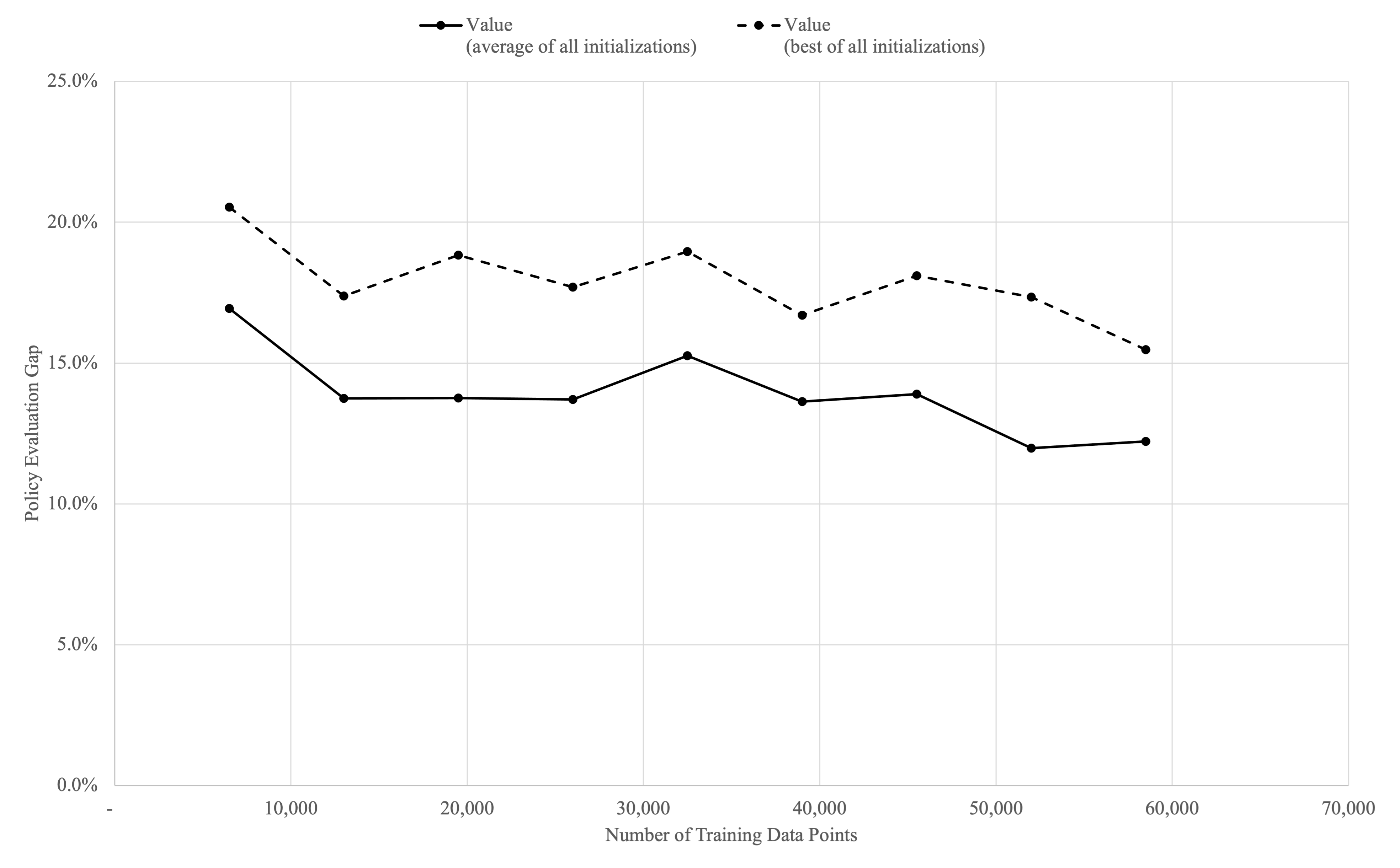
For our computational experiment, policies are evaluated using Monte Carlo simulations. In Figure 5 we compare the evaluation of the base stock policy based on to for different sizes of the dataset . Since the expectation maximization algorithm used to train does not have convergence guarantees, for each dataset size we give the HMM training 5 different random initializations and report both the policy evaluation under the best performing initialization and also the average across the initializations. Since we do not have convergence guarantees in training these HMMs, we see that the gap between the policy evaluations narrows as the training dataset size increases, but then plateaus.
8 Conclusion
We have introduced a specially structured POMDP, the SEP-POMDP, for modeling sequential decision-making environments in the presence of exogenous observations that affect the dynamics and objective of the system. We showed that this class of models inherits optimal value and policy function structural properties from related MDPs, thus extending the deep operations research literature proving such structures for the general MDP and also myriad real-world applications. In a particularly important discussion, we then showed that our formulation encompasses a wide array of supervised learning models for modeling the exogenous uncertainty introduced to the system through the observation process. The range of supervised learning methods is vast and includes: discriminative learning models such as random forests, LOESS, kernel regression, switching regressions, and autoregressive recurrent neural networks; Markovian forecasting models such as Brownian motion, Ornstein-Uhlenbeck processes, and ARMA processes; as well as generative models such as HMMs and Bayesian networks. We gave a sense for the range of applications for which the SEP-POMDP framework can include by discussing its relationship to models from various fields. Finally, we discussed a particular inventory problem under procurement delays, as an illustrative example as to how one might integrate various properties of the SEP-POMDP in a solution procedure. We give additional attention to computational considerations in the appendix.
Much of the reinforcement learning literature is concerned with learning (near) optimal policies through repeated interaction with the decision-making environment, and in many applications in a model-free environment. Developing these methods for learning in the midst of uncertainty is a natural evolution from the foundational MDP that arose out of the operations research community, in which assumptions that the transition probabilities in the system are well-specified are common. What happens, however, when interactions in the environment are expensive, or reinforcement learning requires a number of interactions that pushes the limits of our computing capabilities, as we seek to apply these methods to more and more complex real-world systems? Our reinforcement learning models could benefit substantially by leveraging supervised learning methods for modeling exogenous uncertainty in the system. We see the SEP-POMDP as a potentially foundational modeling framework for building next generation reinforcement learning methods and applications that leverage supervised learning for explaining the uncertainty in the system based on (possibly very large) data.
Appendix A Proof of Inheritance Property
Proof of Proposition 3.
We proceed by demonstrating that P(b) and P(c) hold and then applying Proposition 1. Suppose for all . Recall, we have
By B(a), we have that for all . Further,
as well, since is a space of functions that is a convex cone.
By the same logic, since , B(c) guarantees that P(c) holds as well. The conclusion follows by Proposition 1. ∎
References
- Baum and Petrie, (1966) Baum, L. E. and Petrie, T. (1966). Statistical inference for probabilistic functions of finite state markov chains. The annals of mathematical statistics, 37(6):1554–1563.
- Bertsimas and Kallus, (2020) Bertsimas, D. and Kallus, N. (2020). From Predictive to Prescriptive Analytics. Management Science, 66(3):1025–1044.
- Bertsimas and McCord, (2019) Bertsimas, D. and McCord, C. (2019). From predictions to prescriptions in multistage optimization problems.
- Bishop, (2006) Bishop, C. M. (2006). Pattern recognition. Machine learning, 128(9).
- Bishop, (2019) Bishop, R. R. (2019). Developing Trust and Managing Uncertainty in Partially Observable Sequential Decision-Making Environments. PhD thesis.
- Bismut, (1978) Bismut, J. (1978). An Introductory Approach to Duality in Optimal Stochastic Control. SIAM Review, 20(1):62–78.
- Brown et al., (2010) Brown, D., Smith, J., and Sun, P. (2010). Information Relaxations and Duality in Sotchastic Dynamic Programs. Operations Research, 58(4):785–801.
- Christiansen et al., (2020) Christiansen, R., Peters, J., et al. (2020). Switching regression models and causal inference in the presence of discrete latent variables. J. Mach. Learn. Res., 21:41–1.
- Eddy, (2004) Eddy, S. R. (2004). What is a hidden markov model? Nature biotechnology, 22(10):1315–1316.
- Gelman et al., (2004) Gelman, A., Carlin, J. B., Stern, H. S., and Rubin, D. B. (2004). Bayesian data analysis.
- Hauskrecht, (2000) Hauskrecht, M. (2000). Value-Function Approximations for Partially Observable Markov Decision Processes. Journal of Artificial Intelligence Research, 13:33–94.
- Hyndman and Khandakar, (2008) Hyndman, R. J. and Khandakar, Y. (2008). Automatic time series forecasting: the forecast package for r. Journal of statistical software, 27(1):1–22.
- Jebara, (2012) Jebara, T. (2012). Machine learning: discriminative and generative, volume 755. Springer Science & Business Media.
- Jiang and Powell, (2015) Jiang, D. R. and Powell, W. B. (2015). An Approximate Dynamic Programming Algorithm for Monotone Value Functions. Operations Research, 63(6):1489–1511.
- Kaelbling et al., (1998) Kaelbling, L. P., Littman, M. L., and Cassandra, A. R. (1998). Planning and Acting in Partially Observable Stochastic Domains. Artificial Intelligence, 101(1-2):99–134.
- Lovejoy, (1991) Lovejoy, W. S. (1991). Computationally Feasible Bounds for Partially Observed Markov Decision Processes. Operations Research, 39(1):162–175.
- Malladi et al., (2018) Malladi, S., Erera, A., and White III, C. C. (2018). A Partially Observed Inventory Control Problem. In Review.
- Malladi et al., (2020) Malladi, S. S., Erera, A. L., and White III, C. C. (2020). A dynamic mobile production capacity and inventory control problem. Iise Transactions, 52(8):926–943.
- Nascimento and Powell, (2010) Nascimento, J. and Powell, W. (2010). Dynamic programming models and algorithms for the mutual fund cash balance problem. Management Science, 56(5):801–815.
- Pineau et al., (2003) Pineau, J., Gordon, G., and Thrun, S. (2003). Point-based value iteration: An anytime algorithm for POMDPs. Proceedings of International Joint Conference on Artificial Intelligence.
- Porteus, (1975) Porteus, E. L. (1975). On the Optimality of Structured Policies in Countable Stage Decision Processes. Management Science, 22(2):148–157.
- Puterman, (2010) Puterman, M. L. (2010). Markov Decision Processes: Discrete Stochastic Dynamic Programming. Hoboken: John Wiley & Sons.
- Rabiner, (1989) Rabiner, L. R. (1989). A tutorial on hidden markov models and selected applications in speech recognition. Proceedings of the IEEE, 77(2):257–286.
- Resnick, (1992) Resnick, S. I. (1992). Adventures in stochastic processes. Springer Science & Business Media.
- Rogers, (2007) Rogers, L. (2007). Pathwise Stochastic Optimal Control. SIAM Journal on Control and Optimization, 46(3):1116–1132.
- Ross et al., (2011) Ross, S., Pineau, J., Chaib-draa, B., and Kreitmann, P. (2011). A bayesian approach for learning and planning in partially observable markov decision processes. Journal of Machine Learning Research, 12(5).
- Salinas et al., (2020) Salinas, D., Flunkert, V., Gasthaus, J., and Januschowski, T. (2020). Deepar: Probabilistic forecasting with autoregressive recurrent networks. International Journal of Forecasting, 36(3):1181–1191.
- Sandikci et al., (2008) Sandikci, B., Maillart, L. M., Schaefer, A. J., Alagoz, O., and Roberts, M. S. (2008). Estimating the Patient’s Price of Privacy in Liver Transplantation. Operations Research, 56(6):1393–1410.
- Sandikci et al., (2013) Sandikci, B., Maillart, L. M., Schaefer, A. J., and Roberts, M. S. (2013). Alleviating the Patient’s Price of Privacy Through a Partially Observable Waiting List. Management Science, 59(8):1836–1854.
- Smallwood and Sondik, (1973) Smallwood, R. D. and Sondik, E. J. (1973). The Optimal Control of Partially Observable Markov Processes over a Finite Horizon . Operations Research, 21(5):1071–1088.
- Smith and McCardle, (2002) Smith, J. E. and McCardle, K. F. (2002). Structural Properties of Stochastic Dynamic Programs. Operations Research, 50(5):796–809.
- Sobel, (1981) Sobel, M. (1981). Myopic Solutions of Markov Decision Processes and Stochastic Games. Operations Research, 29:995–1009.
- Sondik, (1978) Sondik, E. J. (1978). The Optimal Control of Partially Observable Markov Processes over the Infinite Horizon: Discounted Costs. Operations Research, 26(2):282–304.
- Spaan and Vlaasis, (2005) Spaan, M. T. and Vlaasis, N. (2005). Perseus: Randomized Point-based Value Iteration for POMDPs. Journal of Artificial Intelligence Research, 24:195–220.
- Topkis, (1978) Topkis, D. M. (1978). Minimizing a Submodular Function on a Lattice. Operations Research, 26:305–321.
- Treharne and Sox, (2002) Treharne, J. and Sox, C. (2002). Adaptive Inventory Control for Nonstationary Demand and Partial Information. Management Science, 48(5):607–624.
- Tryphon and Lindquist, (2013) Tryphon, T. G. and Lindquist, A. (2013). The Separation Principle in Stochastic Control, Redux. IEEE Transactions on Automatic Control, 58(10):2481–2494.
- Watson, (1994) Watson, M. W. (1994). Vector autoregressions and cointegration. Handbook of econometrics, 4:2843–2915.
- West and Harrison, (2006) West, M. and Harrison, J. (2006). Bayesian forecasting and dynamic models. Springer Science & Business Media.
- Zhou et al., (2009) Zhou, E., Lin, K., Fu, M. C., and Marcus, S. I. (2009). A numerical method for financial decision problems under stochastic volatility. In Proceedings of the 2009 Winter Simulation Conference (WSC), pages 1299–1310.
- Zipkin, (2008) Zipkin, P. (2008). On the Structure of Lost-Sales Inventory Models. Operations Research, 56:937–944.
Figures
- 1.
Generate a finite set of belief points, , via belief trajectory simulation (as in Appendix E). Let .
- 2.
For each , generate demand trajectories . This gives us an estimate of the probabilities we need to compute the base stock level :
- 3.
Calculate the estimated base stock level, , for each :
(10) - 4.
Generate the separating hyperplanes by training a multi-class linear, soft-margin SVM on the set of tuples .
Evaluate(, , , , , , , , ): For each Monte Carlo simulation , generate as follows.
- 1.
Initialize , , , , and . Sample from the belief distribution .
- 2.
For :
- •
Determine ordering decision and cost.
- •
Transition, costs, and belief update.
- •
Return:
Appendix A Relationship to Statistics and Machine Learning
A.1 Markov Forecasting Models
Brownian motion. We might consider modeling the auxiliary process (which we briefly assume to be univariate), , as standard Brownian motion, which satisfies the following two properties (Resnick, 1992, chapter 6): (1) has independent increments and (2) . In our notation, the conditional probability distribution is:
Standard Brownian motion satisfies the Markov assumption, by virtue of its independent increments, as do other examples of Lévy processes. In fact, the Markov assumption holds for other generalizations built upon standard Brownian motion that are popular particularly in mathematical finance (we will discuss one such application from Zhou et al., 2009, later), for example, Brownian motion with drift, geometric Brownian motion (popularized by its use as a model of the underlying stock price process in the Black-Scholes model), and Ornstein-Uhlenbeck processes (Resnick, 1992, Zhou et al., 2009). For standard Brownian motion and these generalizations, there exist Markovian extensions in the case of a vector-valued auxiliary process, enabling modeling flexibility with correlated auxiliary data.
Autoregressive time series models. Autoregressive time series models are some of the more popular forecasting models used in practice for time series with regular and discrete time intervals (Hyndman and Khandakar, 2008). For example, the modeler might assume that the auxiliary process is an “autoregressive moving average” process, with parameters and (call this ARMA) determining that for all , is dependent upon the past realizations of the auxiliary data process, , and the average of the previous realizations of the noise process :
Note that is Markovian with respect to the vector . Let be the previous observations of the auxiliary process before time and let be the previous observations of the -process. Since the -process is assumed to be i.i.d., satisfies the forecasting conditional probability of (5) with fixed parameters :
and the following marginal conditional distribution over is normally-distributed:
This kind of autoregressive model can be extended to the case of a vector-valued auxiliary process in the vector autoregressive (VAR) model (Watson, 1994).
Appendix B Monotone Approximate Dynamic Programming
Consider the finite horizon MDP model considered in Jiang and Powell, 2015, which we succinctly describe by the following Bellman equation (and without loss of generality, we assume a minimization formulation, to more easily facilitate comparison to our SEP-POMDP framework):
where the state transition dynamics are described by the stochastic function, and is a stochastic process (which Jiang and Powell, 2015 call the “information process”), in a space , meant to capture the totality of the stochasticity in state dynamics. Now, we note that this MDP formulation corresponds to the MDP analogs of (3) (albeit with a description of state dynamics via a stochastic function, rather than the equivalent conditional probability specification). The only difference is the introduction of an affixed value of the observation process, :
| (11) |
where . We might consider as introducing an observed component of the information process, which in the MDP analog formulation is affixed, but for the SEP-POMDP we permit to be a random variable that is useful for explaining (at least part) of the uncertainty captured by the information process, and for which we want to build a statistical learning model for describing, as in Section 5.
Jiang and Powell, 2015 are principally focused on MDPs for which the optimal value functions exhibit the following monotonicity property, for all :
| (12) |
where is a component-wise partial order, such that when the state can be decomposed into (where is in a space and in a space ):
They present a proposition with sufficient conditions under which the optimal value functions exhibit the monotonicity property (12), that we include verbatim, below, with only trivial modifications to facilitate comparison to our MDP analog formulation (11). We then demonstrate that the assumptions of this proposition guaranteeing monotone value functions for the MDPs in Jiang and Powell, 2015 satisfies the conditions of Corollary 3, and thus the SEP-POMDPs that include statistical learning models for explaining the -process (an observed component of the information process of Jiang and Powell, 2015) inherit this monotone value function structure.
Proposition 6 (Jiang and Powell, 2015, Proposition 1).
Suppose that every can be written as for some and , and let , be the state at time , with and . Assume:
- JP1.
For every with , , and , the state transition function satisfies ,
- JP2.
For each , , with , and , and .
- JP3.
For each , and are independent.
Then the value functions satisfy the monotonicity property (12).
We will prove the following inheritance proposition, proving SEP-POMDP inheritance of monotone optimal value function structure under conditions JP1-JP3.
Proposition 7 (SEP-POMDP inheritance under Jiang and Powell, 2015 monotonicity conditions.).
Suppose JP1, JP2, and JP3 hold. Then, for the SEP-POMDP , for , satisfies the monotonicity property for all . That is, for :
Proof of Proposition 7.
It suffices to show that JP1-JP3 imply P(a), B(a), and B(b). We begin by explicitly defining the structured functional spaces (implicit in Jiang and Powell, 2015):
The space of real-valued monotone functions is closed, so P(a) is satisfied. To show that B(b) holds, we utilize the results of Smith and McCardle, 2002 and note that the functions in satisfy a special kind of joint extension of a C3 property, , called single-point properties (for minimization problems, e.g. monotonicity, concavity in ). Since the monotonicity property defining is a single-point property, it follows from Smith and McCardle, 2002 Proposition 4 that it is preserved under minimization. Finally, B(a) is satisfied by the following inductive argument (from Jiang and Powell, 2015) following from JP1 and JP3. Suppose and such that :
Hence, . By JP2, . B(a) follows because is a convex cone. ∎
Appendix C Computational Example
C.1 Proof of base stock optimality.
We will prove Proposition 5 — the optimality of a base stock policy for the single product inventory replenishment problem under procurement delays — by showing how, since the problem can be formulated as a SEP-POMDP, it inherits this structure from an MDP analog. Rather than showing this directly, considering the context of an MDP analog inventory problem, we instead show conditions for SEP-POMDPs inheriting a more general myopic optimal policy structure from the MDPs considered in Theorem 1 of Sobel, 1981, and then demonstrate that our computational example satisfies the conditions for this myopic optimal policy structure.
We will make use of the notion of separable functions.
Definition 3.
(separable function) A function is separable if there exists a function and a function such that .
Note that the space of separable functions is a convex cone. That is, suppose we have two separable functions, and , which map to , and conic weights . Clearly,
Now, we prove conditions for the optimality of myopic policies for the SEP-POMDP, that are inherited from the MDPs of Sobel, 1981, and we assume the spaces , , , and are discrete.
Proposition 8 (Myopic optimal polices.).
Suppose the following:
- (i)
such that , for all , ,
- (ii)
is independent of (and so we express as ), for all ,
- (iii)
, where
- (iv)
is feasible for all
Then, the stationary deterministic policy for all is optimal.
Proof of Proposition 8.
Suppose for all . We begin by defining the following structured function spaces:
We want to show that there exists a set such that for all is stationary optimal by showing that P(a), B(a), B(b), and B(c) hold.
P(a) holds trivially. We aim to show B(a) holds. Suppose . Observe that (i) and (ii) are equivalent to for all and for all , which imply that
B(b) trivially holds. Further, separable functions when minimized yield state-invariant optimal policies (maximizing over is equivalent to minimizing over for all ). So B(c) holds. By Proposition 3 we conclude that there exists a set such that for all is stationary optimal.
It remains to show that for all , the myopic minimizer of the function . An inductive argument, which follows along the lines of the proof given in Sobel, 1981 proves this result.
Let and . The value function of the SEP-POMDP, under any policy is defined as follows, where and :
| (13) | ||||
| (14) |
and where (3) follows from application of assumption (a). From assumption (b), , where is a random variable depending only on and . Then,
We conclude that the policy for all , is stationary and optimal. ∎
Now, we can prove the optimality of the base stock policy in Proposition 5 by showing that it satisfies the conditions of Proposition 8 as a myopic optimal policy.
Proof of Proposition 5.
We go case-by-case through the assumptions of Proposition 8.
- (i)
- (ii)
In the inventory position formulation, the dynamics of the inventory position are defined by the stochastic difference equation, , and do not depend on .
- (iii)
This is the definition of the base stock levels in Equation 10, where from , above.
- (iv)
This condition is guaranteed by the attainability condition of Proposition 5, namely: for all .
Since of Proposition 8 are satisfied, the base stock (myopic) policy defined by Equation 10 is optimal. ∎
Appendix D Computational Tractability
POMDPs are notoriously difficult to solve for other than small instances due to the fact that the belief space contains an uncountably infinite number of possible belief vectors. There have been various approaches in the literature that seek to overcome the tractability issue of the POMDP. In this appendix we discuss additional types of solution procedures for POMDPs — belief trajectory simulation, exact, information relaxation, and online heuristics — and give examples of how the specialized structural properties of the SEP-POMDP can be utilized within these frameworks to solve (or approximately solve) SEP-POMDPs.
D.1 Belief Trajectory Simulation Methods
Belief trajectory simulation methods are based upon the intuition that, for many problems, there are only a small subset of beliefs that are reachable under an optimal policy. Various approaches in the literature successively build a grid on by alternating at each epoch between sampling new beliefs and performing value iteration operations on the new belief states (Pineau et al., 2003, Spaan and Vlaasis, 2005).
Here we present an a priori belief trajectory simulation method for constructing a discrete grid approximation, , which utilizes the actual dynamics of the modulation and observation processes, while alleviating the computational burden associated with past approaches for the generalized POMDP due to the fact that learning in SEP-POMDPs is passive and independent of control. This method turns solving the SEP-POMDP into solving a completely-observed MDP with state space .
Suppose we have a metric space , where is the sup-norm and is the belief space. Let , the grid of points in rounded to the -th digit. Note that . We detail the so-called solution procedure for SEP-POMDPs.
- 0.
Initialization. Initialize belief distribution, modulation state, number of simulation runs, mesh parameter, and cardinality parameter — , , , , and respectively.
- 1.
Belief simulation. Generate, according to the sequences and . Then compute recursively such that for .
- 2.
definition. Let be rounded to the -th digit and let , the -th most frequently visited balls of radius in .
- 3.
Solving the MDP with state space . Solve the modified completely observed MDP with optimality equation
where and .
In step 0, we initialize the solution procedure. We note that should be a positive integer and controls the fineness of the grid. The cardinality parameter, , determines how many points will be included in the approximate grid.
In step 1, we simulate a trajectory of the beliefs by simulating the evolution of observations and modulation states according to the underlying Markov chain governing the dynamics, and recursively performing the belief update operations according to these observations and modulation states. So long as the Markov chain for the modulation states is ergodic, simulating one long trajectory should be sufficient for approximating a steady state distribution of modulation states. We note that this step is simulating a passive learning environment since the belief updates are independent of control under the SEP-POMDP conditioning assumptions, guaranteeing that the learning operation for SEP-POMDPs is computationally tractable.
In step 2, we determine , the set of simulated belief states rounded to the -th digit, so that is the unique point in such that is within a ball of radius of . Let . (Note that .) There is a complete order on induced by the binary operator, , defined so that
This order counts the number of simulated beliefs that are rounded to a particular and ranks them. We then define to be the -th most frequently visited rounded beliefs (Note that ). Of course, has cardinality , so it is finite in dimension.
Finally, in step 3 we are left with the SEP-POMDP optimality equation, below
Our remaining challenge is that may not be in for a given . Suppose . The hope is that such that , and that . These assumptions may not hold if either is not near any point in (although intuitively, in most cases, it should be since we chose on the basis of frequently visited belief vectors in our simulation), or if is near a facet of the Sondik regions of , so that is not a good approximation to . There are many ways we could define , such as .
This creates a well-defined MDP, with state space , which serves as our approximate model for the SEP-POMDP. The benefits of this method is that we reduce drastically the number of possible belief states that we need to consider in the SEP-POMDP by using the actual dynamics of the system, which makes it better-suited than uniform or random grid methods for each particular problem instance (Lovejoy, 1991, Hauskrecht, 2000).
D.2 Exact Methods
Exact methods are based upon value iteration and seek to solve the POMDP exactly by utilizing the piecewise linear and concave structure of the value function with respect to to construct the defining facets of the value function. Sondik, 1978 and Smallwood and Sondik, 1973 were the first to take this approach in their seminal papers. Kaelbling et al., 1998 improved upon the complexity of this approach by using linear programming to construct the facet vectors. For the SEP-POMDP this structural result implies that if there is a finite set of vectors for all such that , then there is a finite set for all such that and that in the limit, the fixed point of , , is concave in for all . In analogy to computational procedures that make use of this structural characteristic for the POMDP, the process of constructing for the SEP-POMDP involves an intermediate step, the determination of the sets such that . The computational implications of the inheritance property vary as a function of the structure under consideration and mirror the computational implications of this structure for the MDP analogs. For example, assume the MDP analogs are such that for each , there exists an optimal policy that is monotone in . Then, for each , there exists an optimal policy such that if , then . It is therefore unnecessary to construct for all .
D.3 Information Relaxation and Upper and Lower Bounds
Another common method for approximately solving stochastic dynamic programs is via information relaxation, as in Brown et al., 2010. We give a natural information relaxation-based heuristic here that is based on a relaxation of the partial-observability of the modulation process and can generate both upper and lower bounds on . Suppose we want to minimize the expected total discounted cost, where at each decision epoch the DM has available the information as in the SEP-POMDP, , but also knowledge of the modulation states . Feasible policies map into feasible actions at all epochs . The DM is faced with a MDP defined by the operator , where is the space of bounded real-valued functions on ,
In the following proposition, we show that the fixed point of can be used to determine a lower bound on .
Proposition 9.
for all , where and .
Proof of the proposition follows by straightforward observation that all SEP-POMDP policies in are feasible for this MDP, but not all policies for this MDP are feasible for the SEP-POMDP. We remark that this bound may be improved by applying a proper penalty term, akin to a Lagrangian relaxation, an idea developed in Brown et al., 2010 and Rogers, 2007.
The fixed point of of any policy can serve as an upper bound on , where is determined exactly or approximated by simulation. If is small, then is a good sub-optimal policy. As an example, let be an optimal policy for the MDP having operator . We remark that is determined when the lower bound presented in Proposition 9 is computed. Let be the randomized policy with probability . We would expect this policy to be an excellent sub-optimal policy if observations of the modulation process were highly accurate. As another example, if is the optimal policy generated for the MDP in Step 3 of Figure 2 (a function from to ), then one might consider , where .
D.4 Heuristic Solution Procedure
We now present an alternative, heuristic solution procedure that must be implemented in an online manner. The fundamental idea is to map the SEP-POMDP into a related completely observed MDP with a state space on rather than on . We may assume that is finite in its cardinality, and thus this mapping is a state space dimensionality reduction technique (as is the procedure, above). The tradeoff is that we must solve such an MDP at each time epoch in order to capture the belief dynamics.
- 0.
Initialization. Assume is given. Set .
- 1.
Solve the completely observed MDP for all :
Let be an optimal policy, mapping into .
- 2.
Choose action to equal with probability .
- 3.
Observe the observation (which will equal with probability ). Set .
- 4.
Observe the state (which will equal with probability ).
- 5.
Increment ; go to 1.
The intuition behind the procedure begins with the observation of the following inequality
By pulling the minimization inside the summation, the idea is to establish a lower bound on by solving a related problem. We formalize this intuition in the subsequent proposition. Let
and let be the unique fixed point of .
Proposition 10.
, for all .
Solving for is no more computationally tractable than solving for due to the cardinality of and the dependence of on . In developing our heuristic procedure, we seek an approximation to for a fixed . If we assume is small, then it is reasonable to assume that is close to in many cases. This is effectively a learning rate assumption (that learning is incremental and gradual), and is one that has been made in the literature, e.g. Malladi et al., 2018. We then define a completely observed MDP with state space :
| (15) |
This is the intuition behind step 2 in Figure 7. Since this approximation is for a fixed , it is amenable to an online implementation, where this completely observed MDP is solved for each .
We remark that the following is likely to be a valid inequality (although not necessarily)
where is the fixed point of Equation 15. We use Equation 15 to develop a heuristic that, for a given , chooses action (an optimal policy mapping into , for this approximate MDP) with probability . This randomized policy is a probability matching heuristic.